Eindhoven University of Technology

MASTER

Programming heterogeneous wireless sensor networks

Kalloe, V.A.

Award date:2009

DisclaimerThis document contains a student thesis (bachelor's or master's), as authored by a student at Eindhoven University of Technology. Studenttheses are made available in the TU/e repository upon obtaining the required degree. The grade received is not published on the documentas presented in the repository. The required complexity or quality of research of student theses may vary by program, and the requiredminimum study period may vary in duration.

General rightsCopyright and moral rights for the publications made accessible in the public portal are retained by the authors and/or other copyright ownersand it is a condition of accessing publications that users recognise and abide by the legal requirements associated with these rights.

• Users may download and print one copy of any publication from the public portal for the purpose of private study or research. • You may not further distribute the material or use it for any profit-making activity or commercial gain

Take down policyIf you believe that this document breaches copyright please contact us providing details, and we will remove access to the work immediatelyand investigate your claim.

Download date: 06. Jun. 2018

  

EINDHOVEN UNIVERSITY OF TECHNOLOGY Department of Mathematics and Computer Science 

            

MASTER’S THESIS  

Programming Heterogeneous  Wireless Sensor Networks 

 by 

Amar Kalloe                        Graduation committee:  prof. dr. 

dr. ir. dr.  

 J.J. Lukkien P.H.F.M. Verhoeven C. Huizing 

(Supervisor) 

     

November 4th, 2008

  

    

ABSTRACT 

Wireless sensor networks (WSN’s) are an upcoming technology that integrates miniature computers, called nodes, into an environment.  They are generally used to autonomously monitor an environment and either report data or take an action. An important challenge in applying WSN’s in practice is programming them. Current programming models are either on a low abstraction level or can be used only for homogeneous WSN’s, in which all nodes are the same. Thus, especially programming heterogeneous WSN’s, which are required for many applications, is difficult. The programming model described in this report provides the option of programming heterogeneous WSN’s on a higher abstraction level without a strong increase in energy usage. When implemented, more types of WSN‐applications can be programmed quicker.  For developing applications for a WSN, we created an event‐based language that abstracts over the network, but offers control over individual nodes. For the crucial deployment phase, in which an operational system is created from the developed code, a schema was devised that permits different methods of deployment. This offers additional trade‐offs for cost and flexibility. For the run‐time phase, a process was designed that offers concurrent execution of branches instead of a sequential, instruction‐based interpreter. This reduces waiting time and potentially energy usage.    

ii  

     

   

iii  

     

ACKNOWLEDGEMENTS 

Hereby, I extend my gratitude to the people who aided me in this project. In particular, I would like to thank:  • Johan Lukkien, who entrusted me with this project and whose feedback influenced the way I 

think about systems and design • Richard Verhoeven, who worked with me during  the project, and agreed to serve on my 

committee • Kees Huizing, who agreed to serve on my committee • Remi Bosman, who worked with me during the project and helped me to build a prototype • Harold Weffers, who offered me many words of advice and helped me to structure this thesis • The members of WASP, who offered their experience and views on the project • Arcilio Virginia, who provided me with last‐minute feedback on this thesis • My family, especially for the extra support they gave me during the time I was working both on 

writing my thesis and working at OOTI    

iv  

 

1  

TABLE OF CONTENTS 

1.  Introduction ........................................................................................................................................................................ 2 2.  Analysis ................................................................................................................................................................................. 4 2.1  Key drivers ................................................................................................................................................................. 4 2.2  WSN architecture ..................................................................................................................................................... 5 2.3  Current state ............................................................................................................................................................ 10 2.4  Problem statement ................................................................................................................................................ 15 

3.  Global design ..................................................................................................................................................................... 17 3.1  Development ............................................................................................................................................................ 17 3.2  Deployment .............................................................................................................................................................. 23 3.3  Run‐time .................................................................................................................................................................... 29 

4.  Development ..................................................................................................................................................................... 38 4.1  Example ..................................................................................................................................................................... 38 4.2  General service definition structure .............................................................................................................. 39 4.3  Addressing of nodes ............................................................................................................................................. 41 4.4  Functions ................................................................................................................................................................... 43 4.5  Remote services ..................................................................................................................................................... 44 4.6  Subscriptions ........................................................................................................................................................... 45 4.7  Clustering .................................................................................................................................................................. 46 4.8  Conclusion ................................................................................................................................................................ 47 

5.  Deployment ....................................................................................................................................................................... 48 5.1  Translation to bytecode ...................................................................................................................................... 48 5.2  Bytecode interpreter ............................................................................................................................................ 48 5.3  Conclusion ................................................................................................................................................................ 59 

6.  Run‐time ............................................................................................................................................................................. 60 6.1  Execution method .................................................................................................................................................. 60 6.2  Conclusion ................................................................................................................................................................ 62 

7.  Example ............................................................................................................................................................................... 63 7.1  Cow scenario ............................................................................................................................................................ 63 7.2  Conclusion ................................................................................................................................................................ 67 

8.  Conclusion .......................................................................................................................................................................... 68 9.  References .......................................................................................................................................................................... 70 Appendix A:  Grammar ......................................................................................................................................................... 73 Appendix B:  Conversion to bytecode ............................................................................................................................ 76 Appendix C:  Bytecode instructions ................................................................................................................................ 79  

2  

1. INTRODUCTION Wireless sensor networks (WSN’s) are an upcoming technology that change the way systems can be integrated into an environment. They consist of miniature computers called nodes, which have the ability to measure data from their environment, to wirelessly communicate with other nodes or a base station, to perform computations and in some cases to influence their environment. When combined, the WSN that emerges can monitor an environment and autonomously decide to report certain data to its base station or to take some action.  Drivers Besides monitoring and possibly controlling an environment, the general idea for WSN’s contains some other aspects as well. They should be capable of being deployed into environments that are not easily accessible. Therefore, the network should be able to function without physical human accessibility for a long time, often years. This puts strict requirements on its energy consumption and robustness.  Another aspect is that WSN’s should be very well integrated into their environment. A vision is that they should become ‘smart dust’; nodes should be spread around an environment in large amounts. This places restrictions on nodes’ size and cost. It also implies that nodes can be scattered into an environment and made to work quickly. This should be achieved by making WSN’s easily applicable to a variety of contexts.  These drivers, especially the focus on long lifetime, justify taking an approach that differs from the established methods from PC‐ or common embedded technology. By taking into account the type of applications that WSN’s are developed for, the requirements can be served in a better way.  Current usage Currently, WSN’s are deployed mostly in a few experimental settings. An example is ZebraNet, where the WSN consists of zebra tracking collars which are cheaper and can observe more than previous monitoring systems. Another example is the LOFAR‐Agro project that deploys nodes to detect conditions for a certain potato‐disease. In PIPEnet, the WSN is used to detect water levels, flow, leaks and bursts in water mains.   Focus Many of the current WSN’s are homogeneous, which means that all nodes have the same hardware and software. The Wirelessly Accessible Sensor Populations (WASP)‐project, where this thesis contributed to, has a focus on heterogeneous WSN’s. In such networks, nodes can be equipped with different hardware and perform different tasks. Three cases considered in this project are cow herd health monitoring, elderly care and assisted road transport. In the cow herd monitoring scenario for example, a cow can be monitored by a pH‐sensor in the stomach, a temperature sensor in the ear, a movement sensor around the leg and a position detector around the neck.  Challenges An important challenge in increasing the feasibility of WSN’s is that of increasing their programmability. This will allow them to be more easily deployable and flexible. To influence this, an adequate programming model should be created. Currently, multiple programming models exist that aid in development of applications for WSN’s. Languages that offer the greatest amount of abstraction are the network‐centric programming languages. These allow the programmer to program the behaviour of the network as a whole, instead of programming the behaviour of single nodes. However, many of these languages do not support the heterogeneity required by, for example, the WASP‐project. There is also a split between node‐independent domain‐specific languages, which offer high abstraction, but little control over execution and more general node‐dependent languages, which offer significant control over execution, but less abstraction. Additionally, many of the useful concepts and ideas that occur in different languages do not occur in a single language.  

3  

Goal In this thesis, a programming model for heterogeneous WSN’s is described that addresses the aforementioned gaps. Specifically, the goals of the WASP‐project are taken into account. Therefore, the programming model follows an event‐based approach. It is constructed through a design‐based approach with deployability, flexibility and lifetime as main drivers. Besides specifying how to program a WSN, we also describe how to map such applications to individual node behaviour. However, the focus is on programming behaviour of the WSN, not its raw functionality. Additionally, its operation in lower layers, such as those related to networking, is not described.   The programming model will cover the three phases from getting source code to an operational WSN: development, deployment and run‐time. In each of these phases, distinct design choices have to be made. For the development‐phase, the choices are primarily around the programming language that will be used, with focus on the abstraction level and the type of concepts. The choices for the deployment‐phase revolve around the level of reprogrammability of the node and how this is achieved. For the run‐time phase, we describe how the operational execution can be performed efficiently.   Contributions This is an improvement to the status quo in several ways. Currently, the choice is either between using homogeneous WSN’s or lower‐level programming. The programming model described here, provides the additional choice of high‐level programming of heterogeneous WSN’s. Thus, when implemented and used, more kinds of WSN‐applications can be programmed quicker.   For the development phase, a programming language has been developed that offers both high abstraction and a level of control over execution in heterogeneous WSN’s. For the deployment phase, a schema was devised that permits the programming model to be used for different methods of deployment, each with a different trade‐off. For the run‐time phase, a process was designed that offers concurrent execution of branches instead of a sequential, instruction‐based interpreter.  Overview In Chapter 2, an analysis is provided of WSN domain. It also includes related work on WSN programming models and the problem statement. The global design, in which the most important design choices are discussed, is described in Chapter 3. The following three chapters describe more detailed aspects of the design. Chapter 7 provides an example of how the programming model can be applied to a case. Contributions of this thesis and future work are described in Chapter 8.      

4  

2. ANALYSIS This chapter provides an analysis of wireless sensor networks and states the problem that will be addressed in this thesis.  Wireless sensor networks consist of miniature computers, equipped with sensors, a radio and a battery. The network also includes base stations or gateways which connect the WSN to another network (such as the internet). The nodes can perform the following four functions: 

• Measuring: Through the sensors, extract data from the environment (such as temperature, humidity or light intensity). 

• Computing: Through a processor and memory, perform computations on data (such as averaging, FIR’s or other algorithms). 

• Communicating: Through the radio, transmit and receive data to and from other nodes or a gateway. 

• Actuating: Through actuators (if available), influence their environment (such as turning on a light). 

 As nodes are often deployed in situations in which cabling is difficult, receiving power from a cable is infeasible as well. Therefore, they are equipped with a battery and sometimes with equipment for energy scavenging (such as a solar power panel).   Generally, the nodes are intended to be deployed on a variety of scales (from less than ten to thousands) to monitor an environment. When certain events of interest occur in the network, a report should be sent to the gateway or an actuator should be activated. Determining whether the event is of interest and gathering the required data may require data from multiple nodes around the network. Alternatively, the network may send data to the gateway upon user request.  The key drivers of wireless sensor networks are discussed in the next section. Subsequently, an overview of the current WSN architecture is provided. This is followed by current real‐life examples of WSN usage and the role of the key drivers in these cases. An analysis follows in which aspects that still can be improved are highlighted. Then, the focus is set to programming models and the current state of these in WSN’s. Finally, the problem statement of this thesis is described, which also limits the scope of this thesis.  

2.1 Key drivers WSN’s are driven both by a market demand of such applications as well as by a technology push. The emerging technology is increasing miniaturization of computer technology and the market demands for it are various. The technology is demanded for usage in military, agricultural, environmental and industrial applications. As it is an emerging technology, the actual future usage of WSN’s is still somewhat unclear. However, some general patterns emerge in the projected visions for usage.  In general, the focus of WSN’s is on monitoring their environment and reporting certain interesting data to one or more base stations or gateways. Additionally, some WSN’s may also perform some control over their environment instead of purely reporting.  From the projected application areas, a set of key drivers can be derived which appear to form the most important factors in the research and development of wireless sensor networks.   1. Long lifetime: The WSN should perform its task for a long time; preferably years. Due to its 

intended usage in difficultly accessible locations (near volcano’s, on zebra’s, in cow’s stomachs), the network should be able to operate for a long time without on‐site maintenance. This results in a demand for long life time. For WSN’s, the concept most often used is that of ‘energy’. A node usually receives its energy from a battery and consumes it by performing any of its four functions. Energy usage must be minimized for lifetime to be maximized. 

 

5  

2. Low cost: The WSN and especially its elements should be low cost. One of the visions for WSN’s is that they should be seen as ‘smart dust’; nodes should be able to be distributed in an environment in large amounts. As WSN’s are projected to become part of daily applications, the network itself should be low cost as well.   With low cost, both low cost of purchase and low cost of maintenance are meant. The low cost of purchase implies that both cost of material and cost of development should be kept low. 

 3. Ubiquitousness: The WSN should be able to gather information from all around the 

environment. The projected usage is that of creating ‘intelligent environments’, which implies that node should be easily integrated in an environment. Another intended usage is that of monitoring places that are difficult to access. 

 4. Easily deployable: A WSN should quickly and easily be deployed to solve a problem. In the 

concept of ‘smart dust’, the idea is contained that nodes can be scattered in an environment. Though usually the focus is on deployability of the hardware, the software should be just as deployable for it to be useful. Deployability would then include the software development time needed to use the WSN for the application.  Thus, we can summarize that the network should be easily deployable.  

 5. Flexibility: WSN’s need to address a variety of contexts. The concept of WSN’s is intended as an 

‘all‐in‐one’ solution for different monitoring‐and‐reporting applications. The same concepts that apply for a forest fire monitoring application should apply to an elderly people monitoring application. This results in a demand for flexibility. 

 6. Robustness: WSN should be able to continue to operate correctly when problems are 

experienced. As WSN’s are intended to be embedded in physical environments, various things can occur which can inhibit communication or the operation of nodes. The network as a whole should not be impeded. This is a requirement for robustness. 

 It may be argued that these goals can be accomplished by using established methods from computer science. However, the specific configuration of goals and constraints seem to justify new approaches. In particular, the concept of ‘energy’ is not one that is frequently addressed in established methods. Though there is a relation with ‘performance’, ‘energy’ gives a focus on lifetime. The combination of the focus on ‘low cost’, ‘low energy’ with specific attention to monitoring‐and‐reporting applications open up the possibility of creating specific methods which serve these requirements.  By considering the specific contexts WSN’s operate in, the requirements can be adhered to in a much better way than by using general techniques. This can be achieved by cross‐layer optimizations that take into account the specific application.   The demand for these requirements is currently being addressed by certain technology. The general structure of this technology is described in the next section. 

2.2 WSN architecture In this section, the general architecture of WSN’s is described by discussing the network structure, hardware‐ and software‐elements of nodes and the application life‐cycle. This knowledge is necessary for a proper understanding of the rest of the document,   The general structure of a WSN is shown in Figure 1. The basic element of a WSN is the node: a miniature, resource‐constrained computer (explained later in more detail), which can communicate wirelessly with other nodes and a gateway. This gateway is usually a more powerful computer which provides the connection between the user and the network of nodes. This connection can be direct (user operates the gateway) or indirect (the gateway is connected to another network such as the Internet). Depending on what is required by the user, the gateway can be a full‐fledged PC or a PDA. In some cases, multiple gateways may form part of a WSN. 

6  

 

 Figure 1: A WSN consists of nodes and one or more gateways, connected to a user network  As explained previously, the nodes that form the most important part of the WSN perform mainly four functions: sensing, processing, communicating (both sending and receiving), and (possibly) actuating. The sensing function implies that the node captures data from the environment by means of sensors. This captured data is subsequently processed by the node and depending on the result an actuation or communication is performed. Additionally, the node can receive communication from other nodes and respond to that if required. This behaviour is shown in Figure 2.  

 Figure 2: Behaviour of a node  This behaviour is accomplished by using the hardware of the node shown in Figure 3. The node comes equipped with a number of sensors and actuators for performing the sensing and actuating. For processing, the CPU and on‐board memory is used. Many current nodes have separate program and data memory, corresponding to the Harvard architecture (1). This impacts the reprogrammability of nodes. To perform communication, nodes make use of some type of radio. Often this radio is relatively short‐range, covering in the range of tens to hundreds of meters in good 

7  

conditions. As a wireless node is not connected to an electricity grid by means of a cable, it needs to receive its energy to power itself through either a battery or energy scavenging. This last option means that the node extracts energy from its environment by using energy sources such as light or motion. Generally, communication is the most energy‐expensive function of a node. (2)  

 Figure 3: Hardware elements of a node  To control that hardware, a software stack is required. The general structure of a WSN software stack is shown in Figure 4. At the lowest level, the node operating system is located. It provides basic abstractions over the hardware, such as the sensors and the radio. Usually, the MAC‐protocol of the network communication is implemented on this level as well. Though not occurring always in WSN’s, a middleware can be run on top of the OS. This middleware can provide some higher‐level abstractions, which may include functions such as routing and aggregation. These higher‐level abstractions allow applications to be developed in less time and make them more maintainable and portable. A number of WSN middlewares are discussed in 2.3.4. Either on top of the middleware or directly on top of the OS, the application is run. With some middlewares, this application is not directly executable code, but consists of instructions in the data memory that are processed by the middleware.   

Node operating system

Drivers for hardware

Middleware

Routing

MAC

Aggregation

Services

Application

 Figure 4: Software elements of a node  

8  

To achieve such a fully operational node, an application has to go through the steps shown in Figure 5. Two options for such an application life cycle are shown. In both, the application is first developed by writing code in a programming language. Subsequently, the code is compiled into some form. In the left life cycle, it is compiled into code that is placed in a node’s program memory and can be directly executed. Transferring the code from a PC to the node in this life cycle is usually performed by flashing the node’s memory. This option is the only possibility when the node’s operating system does not permit on‐the‐fly reprogramming and requires a direct, wired connection (e.g. through USB or serial cable) between the node and the PC. When the node OS is capable of reprogrammability, the application can be inserted remotely as well.   In the right life‐cycle, the compilation step does not produce code that can directly be executed, but creates some form of bytecode. This bytecode is then transferred wirelessly to the node which runs an interpreter which is capable of interpreting that code and translating that into node behaviour. The bytecode is placed into the node’s data memory and therefore does not require the program memory to be changed.  

NodeNode

User PC

Development

Compilation

Transfer

Execution

User PC

Development

Compilation

Transfer

Interpretation

Execution

 Figure 5: Two options for a WSN application life cycle. Left: direct transfer of executable code to a node. Right: intermediate, not directly executable code is transferred to a node, interpreted and then executed.  In both life cycles, the three phases shown in Figure 6 can be distinguished. First is the development‐phase in which the application code is written in a programming language. Secondly, this code is translated or compiled to some form and is transferred to one or multiple nodes in the deployment‐phase. This phase is especially important for WSN’s as code needs to be distributed over nodes in an efficient way and choices around reprogrammability are made there. Thirdly, the transferred code is executed on the node such that it is in an operational state.   

9  

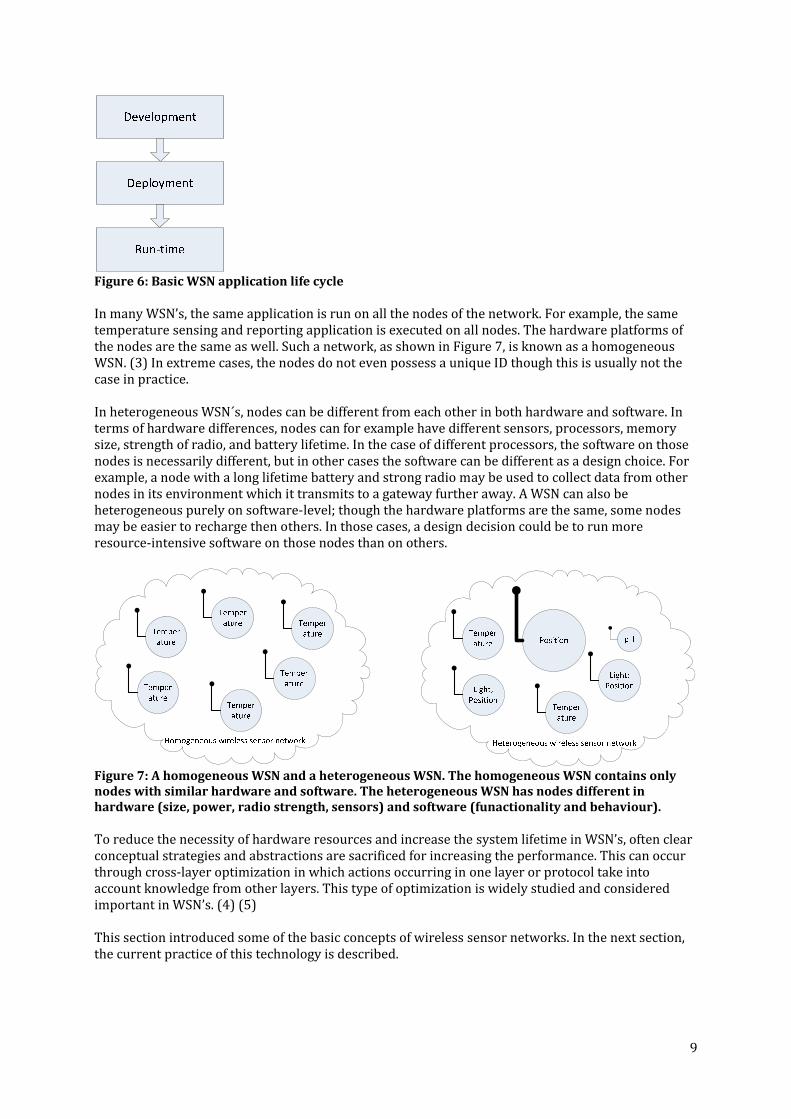
 Figure 6: Basic WSN application life cycle  In many WSN’s, the same application is run on all the nodes of the network. For example, the same temperature sensing and reporting application is executed on all nodes. The hardware platforms of the nodes are the same as well. Such a network, as shown in Figure 7, is known as a homogeneous WSN. (3) In extreme cases, the nodes do not even possess a unique ID though this is usually not the case in practice.   In heterogeneous WSN´s, nodes can be different from each other in both hardware and software. In terms of hardware differences, nodes can for example have different sensors, processors, memory size, strength of radio, and battery lifetime. In the case of different processors, the software on those nodes is necessarily different, but in other cases the software can be different as a design choice. For example, a node with a long lifetime battery and strong radio may be used to collect data from other nodes in its environment which it transmits to a gateway further away. A WSN can also be heterogeneous purely on software‐level; though the hardware platforms are the same, some nodes may be easier to recharge then others. In those cases, a design decision could be to run more resource‐intensive software on those nodes than on others.  

 Figure 7: A homogeneous WSN and a heterogeneous WSN. The homogeneous WSN contains only nodes with similar hardware and software. The heterogeneous WSN has nodes different in hardware (size, power, radio strength, sensors) and software (funactionality and behaviour).  To reduce the necessity of hardware resources and increase the system lifetime in WSN’s, often clear conceptual strategies and abstractions are sacrificed for increasing the performance. This can occur through cross‐layer optimization in which actions occurring in one layer or protocol take into account knowledge from other layers. This type of optimization is widely studied and considered important in WSN’s. (4) (5)   This section introduced some of the basic concepts of wireless sensor networks. In the next section, the current practice of this technology is described. 

10  

2.3 Current state The pursuit of the drivers has led to a number of hardware‐ and software solutions that are being used in real‐life applications. 

2.3.1 Hardware platforms Currently, in pursuing these goals, these current hardware platforms are available. These adhere to the previously described architecture and provide an idea about the scale of hardware resources generally available on a node.  Table 1: Available hardware nodes (Source: (1)) Mote type  Mica  Mica2Dot  Mica2  Telos  ANTS  Imote  uPart Year  2001 2002  2002 2004 2007 2004  N/A Microcontroller     Type  ATmega128 TI 

MSP430 AT

mega128 ARM7DTMI  rfPIC12F675

Program memory  128 KB  48 KB 128 KB 512 KB  1.4 KBRAM  4 KB  10 KB 4 KB 64 KB  64 ByteFrequency  8‐16 MHz 16 MHz 8‐16 MHz 12 MHz  4 MHzStorage Chip  AT45DB041B ST 

M25P80 N/A 

Size  512 KB  1024 KB N/A Communication Radio  TR1000  CC1000 CC2420 (Bluetooth)  (rfPIC)Data rate  40 kbps  38.4 kbps 250 kbps 20 kbps 1 Mbps  40 kbpsPower Minimum supply  2.7 V  1.8 V N/A 3.6 V  3 VTotal power  27 mW  44 mW 89 mW 41 mW N/A 21 mW  35 mW It can be seen from Table 1 that nodes can have between 1.4 and 512KB of program memory and between 64B and 64KB of RAM. The clock speed of their CPU’s is between 4 and 16MHz. Communication is performed at a rate between 20kbps and 1Mbps.   

There is a large difference between different types of nodes and each is suited for a different type of application. The tiny µPart‐nodes for example may be more suitable to ‘smart dust’‐type of applications than the Mica2’s, which may be more suited for more intensive computation and communication. In the future, different types of nodes may be in one network to form a WSN that is heterogeneous in hardware.  These and other nodes are currently in usage in the applications discussed in the next section. 

2.3.2 Current applications  

Though the technology is not in wide use yet, there are a few applications which already utilize the technology. For more information on these examples and others, we refer to (1). An area which has already seen a number of examples is the tracking of wildlife. Princeton University has developed such a WSN for tracking of zebra’s called ZebraNet. (6) With this WSN, a number of zebra’s are outfitted with custom tracking collars with a weight of 1.2kg containing a custom‐made node with a GPS‐device. The position of the zebra is being tracked continuously by the node and is irregularly offloaded to a mobile base station.  Figure 9: Tracking node for ZebraNet 

(39) 

Figure 8: µPart node 

11  

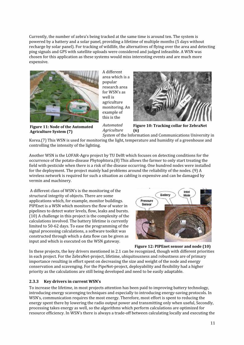
 Currently, the number of zebra’s being tracked at the same time is around ten. The system is powered by a battery and a solar panel, providing a lifetime of multiple months (5 days without recharge by solar panel). For tracking of wildlife, the alternatives of flying over the area and detecting ping signals and GPS with satellite uploads were considered and judged infeasible. A WSN was chosen for this application as these systems would miss interesting events and are much more expensive.   

A different area which is a popular research area for WSN’s as well is agriculture monitoring. An example of this is the 

Automated Agriculture System of the Information and Communications University in 

Korea.(7) This WSN is used for monitoring the light, temperature and humidity of a greenhouse and controlling the intensity of the lighting.  Another WSN is the LOFAR‐Agro project by TU Delft which focuses on detecting conditions for the occurrence of the potato‐disease Phytophtora.(8) This allows the farmer to only start treating the field with pesticide when there is a risk of the disease occurring. One hundred nodes were installed for the deployment. The project mainly had problems around the reliability of the nodes. (9) A wireless network is required for such a situation as cabling is expensive and can be damaged by vermin and machinery.   A different class of WSN’s is the monitoring of the structural integrity of objects. There are some applications which, for example, monitor buildings. PIPEnet is a WSN which monitors the flow of water in pipelines to detect water levels, flow, leaks and bursts. (10) A challenge in this project is the complexity of the calculations involved. The battery lifetime is currently limited to 50‐62 days. To ease the programming of the signal processing calculations, a software toolkit was constructed through which a data flow can be given as input and which is executed on the WSN gateway.  In these projects, the key drivers mentioned in 2.1 can be recognized, though with different priorities in each project. For the ZebraNet‐project, lifetime, ubiquitousness and robustness are of primary importance resulting in effort spent on decreasing the size and weight of the node and energy conservation and scavenging. For the PipeNet‐project, deployability and flexibility had a higher priority as the calculations are still being developed and need to be easily adaptable. 

2.3.3 Key drivers in current WSN’s To increase the lifetime, in most projects attention has been paid to improving battery technology, introducing energy scavenging techniques and especially to introducing energy‐saving protocols. In WSN’s, communication requires the most energy. Therefore, most effort is spent to reducing the energy spent there by lowering the radio output power and transmitting only when useful, Secondly, processing takes energy as well, so the algorithms which perform calculations are optimized for resource efficiency. In WSN’s there is always a trade‐off between calculating locally and executing the 

Figure 12: PIPEnet sensor and node (10) 

Figure 11: Node of the Automated Agriculture System (7) 

Figure 10: Tracking collar for ZebraNet (6) 

12  

calculation on a different node or gateway. Which option is most energy‐efficient depends on the specific situation.  To decrease the cost of the system, the main focus has been on decreasing the cost of nodes. This has been achieved by e.g. using cheap radios and limiting memory.   One of the most important ways of increasing ubiquitousness is making the communication between nodes wireless. Especially in situations where the nodes are mobile this is a primary requirement. Secondly, the size and weight of the nodes are limited. In ZebraNet for example, the node could only be deployed on zebras if the nodes would not hinder the zebras. This factor is also dependent on the cost and robustness of the nodes.   Physical deployability is another important factor with attention paid to properly attaching the nodes to zebras in ZebraNet and adequately burying them into a potato field in the LOFAR‐argo project. To develop the software quickly, most projects use existing operating systems (like TinyOS) and libraries. Though several middleware’s exist for WSN’s, their usage in research projects appears to be quite low.  To increase the ease of flexibility of the WSN, attention has been paid to programming models. In PIPEnet, a custom‐made programming model for the gateways was introduced to facilitate signal processing calculations.  The robustness of a WSN depends on the proper functioning of nodes and on functioning communication between nodes. To prevent nodes from breaking down, they are often packaged well. The robustness of communication is increased by using protocols which take the uncertainty of wireless communication in the environment into account.  There are still several factors which limit the applicability of WSN’s to solve real‐life problems. Those problems can be expressed in terms of the previously mentioned key drivers.   1. Long lifetime: Currently, the lifetime of WSN’s is still limited. WSN’s operating for years without 

maintenance is only possible with energy scavenging from solar power. Operating only on battery power or using other means of energy scavenging has not yet been developed sufficiently to support years of WSN lifetime. 

2. Low cost: As WSN nodes are not yet mass‐produced, the cost per node is still relatively high. Current nodes are in the order of hundreds of euros per node.  

3. Ubiquitousness: The vision of WSN nodes as ‘smart dust’ has not yet materialized. Increased miniaturization is required to accomplish this. 

4. Easily deployable: WSN’s are not yet easily deployed. One of the causes is that they are still very difficult to program. Though there are many algorithms, protocols and middlewares available, there is little integration of these as of yet. WSN programming also currently requires a lot of specialist knowledge about specific hardware platforms, algorithms and protocols that is not easily available.  

5. Flexibility: Once a WSN is programmed for a certain task, it becomes difficult to make modifications. The code is often programmed with much regards to very context‐specific performance and not towards flexibility. Often, the code is not easily transferred to different hardware platforms as well.  

6. Robustness: Currently operating WSN’s face difficulties around reliability. The difficulties of wireless communication and nodes operating in harsh environments are still hard to overcome. 

 A number of these issues are related to programmability. Programmability is the degree of effort required to program a system to perform a certain task. From the key drivers, especially the drivers ‘easily deployable’ and ‘flexibility’ are related to programmability.  

13  

2.3.4 Programming models Every system is programmed by using a programming model. A programming model is a set of concepts, primitives and combinators to express a computation. (11) A programming language will form part of the programming model, but ‘programming model’ is more general. They can operate on different levels of abstraction. A programming model can for example be made to facilitate programming a single processor, a single system or an entire network. For a programming model to be usable, it should include a programming language and a mapping of a program to operation.   To improve the programmability (and thus deployability and flexibility) of a WSN, effort should be spent on improving its programming model. Programming models used in other types of systems (such as PC’s) are less suited for WSN’s as though in conventional distributed programming individual machines are by themselves powerful systems, this is not true for wireless sensor nodes. Additionally, much more than in regular computer systems the value of a sensor network comes from collaboration among the nodes.(12) For optimal programmability and performance of WSN’s it is necessary to match the concepts of the programming model with those required for a WSN application.  There already exists work on programming models on wireless sensor networks. These have differing goals, methods and levels of abstraction. Some programming models can work on top of each other. A taxonomy of WSN programming models has been shown in Figure 13, which has been cited in part from (13). Some aspects from the literature review are more explicitly described in (12). For additional survey papers on current WSN programming models, we refer to (14).   

 Figure 13: Taxonomy of wireless sensor network programming models (source (in part): (13))  

Operating system On the lowest level of abstraction, there are the programming models associated with node operating systems. The popular TinyOS‐operating system is associated with the nesC‐programming language (15), which is based on event‐based concurrency. In nesC, the programmer builds components along with their interfaces, Applications are built by composition of these components. The operating system is kept simple and does not provide the programmer with features such as memory management or a scheduler. The level of abstraction is sufficient enough to be generally portable to other hardware platforms.   FreeRTOS (16) is a more traditional operating system that features multithreading, memory management and synchronization. Programming applications on top of this operating system is done in C. Both these operating systems do not permit remote modification of running code. The SOS embedded operating system (17) is designed for remote reprogrammability. By using a modular structure, parts of the code in the program memory can be replaced remotely. It is programmed using C. 

14  

Support The supporting programming models are built on top of an operating system to provide the developer with some extra facilities and generally do not contain any major additional abstractions over nodes or their sensor data. The programming languages specified under Composition, Sensorware (18) and SNACK (19), provide the programmer with libraries through which applications can be built on a higher level. Under distribution & safe execution, there are solutions which provide solutions to remotely reprogram a node and to wirelessly distribute code over a WSN.   Maté (20), for example, contains a virtual machine running on TinyOS that executes code consisting of special instructions. This allows for very compact applications and reprogrammability. It forms the basis for the ASVM‐approach (2), which proposes application‐specific virtual machines, where functionality available on a node is dependent on the specific application. Their studies indicate that though their interpreter provides significant overhead, its effect on total system lifetime in common applications is neglible due to the cost of other factors such as communication.   Impala (21) is a middleware which provides automatic run‐time adaption to optimize performance, energy efficiency and reliability. It is used in Zebranet. SwissQM (22) is able to provide methods for compact code and reprogrammability using a virtual machine as well, but provides some additional abstractions for communication and data acquisition. However, it is not intended that the developer immediately develops for this virtual machine; the application is developed in a different language such as TinySQL which is compiled into bytecode at the gateway. 

Abstraction The category Abstraction contains the higher‐level programming models which provide abstractions over nodes or their sensor data. The most important distinction here is of that between network‐centric and node‐centric programming models. Network‐centric programming, also known as macroprogramming, allows “application designers to write code in a high­level language that captures the operation of the sensor network as a whole.” (23), Thus, an application is specified as a task that the entire network should perform. In contrast, node‐centric programming means that the application is specified in terms of behaviour of a single node. Additional information about this distinction can be found in 3.1.1.   Within the node‐centric languages, in which programming takes place on node‐level, a distinction can be made between data‐centric and geometric languages. The geometric‐centric languages provide abstractions over nodes based on their location, while the data‐centric languages abstract over other types of data. A data‐centric language, EnviroSuite (24), provides the programmer with an abstraction over physical entities which the nodes track. This is performed by creating objects, to which sensors can be linked through certain algorithms. It is en extension that can be added to existing languages; it has currently been implemented on top of nesC. Hood (25), a geometric‐centric language, creates abstractions of neighbourhoods of nodes. Such a neighbourhood is defined by hop‐range from a node along with the data that should be shared in that neighbourhood. The communication and synchronization is then abstracted over.   Within the network‐centric programming languages, the node‐independent and the node‐dependent languages can be distinguished. The node‐independent languages abstract wholly over nodes; they do not occur as a primitive in the language. In TinyDB (26) for example, the network is presented as one database on which a user can perform SQL‐like queries to retrieve information. Most of the logic of the system is performed at the gateway, while the nodes themselves run very simple interpreters. To make the abstraction towards a database, the assumption is made that each node has equivalent capabilities (homogeneous network). Cougar (27) uses a similar approach.   On the other hand, we have the network‐centric, but node‐dependent programming languages. In these languages, applications are programmed at network‐level, but in which nodes occur as primitives. In Kairos (13) for example, nodes are identified with an integer and operations can be performed on lists of nodes. Some of the mechanisms offered are the identification of one‐hop neighbours, accessing a variable on a remote node and synchronization. The language itself uses a C‐

15  

like syntax. Regiment (28) is a node‐dependent language as well, but uses a functional programming syntax. Nodes are represented using region streams, which are “spatially distributed, time‐varying collections of node state.” In the database‐approaches such as TinyDB, the goal was to provide an abstraction to the programmer to express sensing/monitoring‐type of applications in. In contrast, the goal of Kairos and Regiment is to provide a language to express a wide range of applications in, including building routing trees or general parallel computations. 

Conclusion Concluding, it can be observed that there is a wide variety of available programming models for WSN’s available. Differences between them can occur on purpose, level of abstraction, implementation, restrictions and a variety of other points. In general, important trends appear to be abstraction over the communication layer and offering reprogrammability through an interpreter. However, even with this number of available programming models there are several aspects still missing in the field.   For example, many of the macroprogramming languages treat the WSN as a homogeneous entity and do not support WSN’s in which nodes with different sensors and different functionality occur (heterogeneity). Additionally, on one hand there are the node‐independent languages which offer high abstraction and focus on monitoring applications, but offer little control over execution. On the other hand, there are the node‐dependent languages which offer significant control over execution but offer less abstraction in order to support more general applications. There do not appear to be programming languages with combine the ease of node‐independent programming with the control offered by the node‐dependent languages.  Even though a union of all these programming models would offer quite an encompassing programming model, the field suffers from a lack of integration. Important features such as data‐based addressing, reprogrammability, support for heterogeneity and macroprogramming do not occur together. There appears to be room for a programming model which has flexibility in reprogrammability and usage for different monitoring type of applications, can quickly be used to assemble applications for easy deployment through high abstraction and which offers long lifetime and low cost through low overhead. Addressing this gap is the goal of this thesis. 

2.4 Problem statement In this report, the goal is to develop a programming model for heterogeneous wireless sensor networks with a mapping to individual node behaviour. This programming model focuses on increasing the capability of WSN’s to be used for its purpose. To accomplish this, it should be congruent with the WSN’s purpose and key drivers. Specifically, the programming model should address the goals of the WASP project. As part of this project, an event‐based approach should be followed.  For the WSN’s purpose, the focus remains on the monitoring‐and‐reporting type of applications. The WSN takes its input from sensing the environment, processing this data, and reporting it to a base station or performing some actuation.  The programming model should contribute to the domain by addressing the previously discussed key drivers. This can be achieved by adding little overhead and using energy‐saving techniques to keep the lifetime long. Low overhead should also result in keeping the nodes’ hardware resources low and thus low cost. The deployability should be addressed by making the development time of the software of the WSN as low as possible. Therefore, it is necessary to focus on easy programmability. The programming model should also be flexible enough to fit into the variety of contexts WSN’s can operate in. Additionally, it should incorporate trade‐offs surrounding robustness and reliability. 

Constraints The programming model in this report will focus on programming the behaviour of a WSN on application‐level. The raw functionality, such as the sampling of a temperature sensor on a node, is 

16  

assumed to be pre‐programmed and usable by the programming model. Additionally, the layers below the programming model (such as operating system and network stack, see 2.2) are assumed to be in place. Additionally, routing or other network issues will not be addressed in this report. Therefore, issues surrounding cross‐layer optimization for this programming model will not be discussed in‐depth as well.  To construct this programming model, a design‐based approach is taken. First, we determine what needs to be designed for a WSN programming model. Subsequently, for each identified phase a solution is presented with argumentation derived from the key drivers. 

Description As discussed in 2.2, a WSN consists of sensor nodes connected with user‐systems through a gateway. For a programming model, an application can be considered to go through three phases to go from source code to working system. The common sequence of development is that of writing the code on a user‐system, compiling this to some form, transferring it to the nodes and executing it there. In this process, we distinguished the three phases:  1. Development: The code is written. 2. Deployment: The code is transferred to the nodes in some form (can be compiled first). 3. Run­time: The code is executed on the nodes such that the node is in an operational state.  In each of these phases, distinct design choices have to be made. For the development‐phase, the choices are primarily around the programming language that will be used, with focus on the abstraction level and the type of concepts. The choices for the deployment‐phase revolve around the level of reprogrammability of the node and how this is achieved. For the run‐time phase, we describe how the operational execution can be performed efficiently. In the next chapter, a global overview of the design is provided. The design is described in more detail in the three chapters after.   In this detailed design, a programming language for a WSN will be provided with formal descriptions of its syntax and informal descriptions of its semantics. A mapping will be provided by describing the translation steps that are required to translate a program down to individual node behaviour.   A prototype x86‐implementation of the compilers and interpreters are constructed as well to verify the functional correctness of the model.      

17  

3. GLOBAL DESIGN In this chapter, the global design of the WSN programming model is discussed. For all the three phases identified in 2.2 that bring an application from idea to operational system, the major design choices of the programming model are described. First is the development phase, in which the program code is written. When this is completed, deployment takes place. In this phase, the program code is deployed onto the nodes and the nodes are deployed in the field. After deployment, the WSN is fully operational in the run‐time phase. All of these phases form part of the programming model. More detailed design decisions made for the programming model are further discussed in chapters 4, 5 and 6.  

3.1 Development During the development phase, the applications are programmed by the developer. This requires those applications to be in a human‐readable form. Therefore, at this stage, they exist as program code written in a human‐readable programming language on a user‐system. Therefore, the main choices in this phase are around the design of the programming language.  Designing a programming language requires many choices to be made; our focus will primarily be on the choices that are peculiar to WSN’s and less to the issues that are common to all programming languages (such as typing). The most important choices are discussed in this chapter, while more detailed choices are discussed in Chapter 4.  The first design decision that is discussed is around the level of abstraction of the programming language. 

3.1.1 Level of abstraction 

As discussed in 2.3.4, there are several ways that a WSN can be viewed from a programming language‐perspective. When a WSN is viewed as a monolithic entity, as shown in Figure 14, this may give rise to a node‐independent macroprogramming language. Thus, the network is viewed as one system without explicit distinctions between nodes. This generally provides a high level of 

abstraction, as the nodes themselves are abstracted over. The network becomes abstraction layer.   Such an abstraction may convenience developers who do not wish to concern themselves with specific information of nodes, but who are more interested in information about the network. However, abstracting over nodes can create difficulties when the developer requires insight into the nodes to assign specific tasks to nodes with certain capabilities. Thus, for heterogeneous WSN’s, this solution offers some difficulties. When an application is written without regards to nodes and their capabilities, a complex distribution algorithm for application parts to network is required. Especially for a dynamic network, in which nodes can move, appear and disappear, this will most likely cause significant overhead.  To reduce the need for such a complex algorithm, which will probably have a significant negative effect on lifetime and cost, a programming model with more control over nodes is considered.   

 Figure 14: Macroprogramming  

Wireless Sensor Network

Gateway

CompiledmacroprogramWSN output

Node

User Macroprogram

Node

Node

18  

Such a programming model could be achieved by viewing the WSN as a collection of nodes. This vision can be developed towards a node‐based programming model that is illustrated in Figure 15. This model offers a lower level of abstraction than macroprogramming, but is advantageous when more insight into nodes is required. It also offers more control over where applications are executed. However, performing functions over the entire network is difficult as every action is viewed from the perspective of a single node. This does not have such a positive effect on the ease of programmability of the network as macroprogramming. Especially in a heterogeneous WSN, where one conceptual application for the network needs to be written as multiple applications for different nodes, large difficulties for programmability remain. 

  A compromise is node‐dependent macroprogramming. In this model, programming still takes place on a network‐level, but the programmer has a level of control over what happens on which nodes. Therefore, an application can still be developed as one application, easing the programmability. Additionally, giving some control over nodes to the developer reduces the need for complex distribution, thereby keeping the overhead limited. For these reasons, we choose the network‐centric, node‐dependent option for the programming model. However, we consider the option of a node‐independent model to be preferable if the problem of distribution can be solved with low overhead. 

3.1.2 Concepts As discussed before, a programming model is a set of concepts, primitives and combinators to express a computation. In this section, we describe the decisions around the most important concepts and primitives of the programming model.   

Events First, we determine what the actual function of an application in the programming model is. An application we will consider to be a task that the user wishes to perform. We distinguish the two basic options for initiating an action in the network. (29) In the demand‐driven approach, an actor external to the WSN submits a query to the system. The WSN responds to this query by performing some actions and returning the result. In this case, the query can be considered as an application. However, with WSN’s we are often only interested in data when something of interest occurs in the network.   For such cases, there is the event‐driven approach in which the WSN detects events of interest and acts appropriately to it. Originally demand‐driven systems such as TinyDB have also included an option for an event‐based approach. Due to the importance of events in WSN’s and the goals of WASP, we shall focus on this approach.  Often in event‐based approaches, the applications are specified using Event‐Condition‐Action (ECA) rules. The event‐part specifies the event that triggers the rule, the condition specifies the state the system should be in for the rule to fire and the action‐part specifies the action that should be performed when the rule fires. However, in WSN’s, the actual event‐part is usually a timer‐event that triggers an update of sensor values (there are very few other actual events occurring in the system). The associated condition is then a predicate on those sensor values which indicate whether it has been an event of interest and if action should be taken.  As this pattern is so common, we can combine the event and the condition into a single event condition. This event condition is triggered 

UserCompiled

node-basedprogram

Node

Node

Node

Gateway

WSN output

Figure 15: Node­based programming 

19  

when its condition becomes true. The action‐part should trigger the sending of a certain message or an actuation.  Though we considered the event‐part of the ECA‐rule as an event of the system, it can also be considered as an event in the physical environment that the WSN is monitoring (e.g. “explosion occurs”). Such an approach is considered in (30).  However, this still requires a definition in terms of system events and conditions of how the physical event is actually detected by the WSN. Though the additional layer of abstraction becomes useful when complex events (for more information see: (31)) in the physical world are considered, we currently disregard this within this report. This abstraction layer can be accomplished by creating physical event abstractions from system event conditions. 

Subscriptions and services 

In a monitoring application, an event occurring in the WSN usually results in a message being sent to the user. However, there can be multiple users of a system behind different gateways. Additionally, the occurrence of an event may have to be communicated to a different node. Therefore, a node has to be aware of who is interested in the event. This can be accomplished by maintaining a list of subscribers: nodes or other systems that should receive notification when the event occurs. This introduces the publish/subscribe paradigm into the programming model, which is suited for loosely coupled systems.  Such a subscription should be attached to some entity; it could for example be attached to a node, an event or an application. A node, however, could detect multiple events of which only one may be of interest to a subscriber. The application is too large of an entity as well; nodes should be able to subscribe to events that form part of an application. Therefore, a subscription should be attached to an event in a way. However, the event is not the only part of interest to the subscriber; the action (often a message) is important as well. Therefore, we introduce the concept of a service which combines the event condition and the action.   A service is defined by (32) as such: “a mechanism to enable access to one or more capabilities, where the access is provided using a prescribed interface and is exercised consistent with constraints and policies as specified by the service description.” This is congruent with the concept of service that we use: the event with the action is the capability that is accessed and the interface is the subscription and other messages sent by the triggering of an event.  Additionally, the service can be linked to the node which should be responsible for executing the service.  The part about constraints and policies was not addressed yet.  For a WSN service, such policies and constraints relate to the extra‐functional aspects of the service, which are the properties related to sampling and communication. For sampling, the period by which it samples is of prime importance. Often, the user does not require a very accurate sampling period. Therefore, to allow some freedom for optimization by the application, a minimum and a maximum sample period should be specified. For communication, the user is interested in when he receives the message after an event has occurred. This can be specified as a deadline, which is the maximum time a message is permitted to take. Additionally, to aid the system in making trade‐offs between assigning resources to applications, priorities may be specified over the execution and the communication. These parameters can be used as well to influence the robustness of the system by specifying, for example, the drop policy for packets. By specifying such extra‐functional properties, no decision is made by the developer here on which protocols and algorithms to use to accomplish this. These decisions are to be taken on a different level. How this can be performed is out of the scope of this report.  These extra‐functional properties of the service could be specified as properties of the service itself. In that case, a subscription is always for that service with the same extra‐functional properties. However, in many cases a user is interested in an event, but with slightly modified parameters. When these parameters are fixed as part of a service, a new service needs to be defined with those modified parameters, causing inefficiency. To prevent this, these parameters can be made specifiable through the subscription. In such a way, the subscriber can get different extra‐functional demands of the 

20  

same service without reprogramming. This increases flexibility and further abstracts the concept of a service without expressiveness being lost.  

Functions and remote services Within the service, an event condition and action is specified. A question arises on how to express these. What should be expressed is some composition of the basic functionality of the WSN. In the event condition, this functionality should be composed in a way that it implies a condition and in the action‐part it should be composed in such a way that an action is undertaken. Thus, what is required is an appropriate abstraction of functionality. In our problem statement described in 2.4, we assumed that the programming model is intended for programming behaviour on top of in‐built functionality. For this in‐built functionality, we will consider functionality such as sampling a sensor and sending data to subscribers as this will be common to most applications. These can be abstracted over by means of a function, which takes parameters as input and which possibly returns a value.   Subsequently, it has to be decided what else should be abstracted as a function and what should arise as behaviour from a composite of functions. For example, functionality such as averaging of data over multiple nodes or over time is both complex and common. For ease of programmability, it would be advantageous if functionality that is commonly used in applications is expressed in terms of a function. However, this has a negative effect on cost (when the WSN itself has to contain a large number of pre‐programmed functions, this requires memory) and flexibility (when only a limited number of functions is offered, not all computations will be expressible).   As our main focus is on monitoring applications, we choose to sacrifice flexibility by offering only functions related to this domain. Additionally, the functions available in the WSN can even be limited to the functions related to that sub‐domain. The concept that emerges then is rather similar to that of ASVM (2) discussed in 2.3.4. Furthermore, in a heterogeneous WSN not all functions have to be available on all nodes. This is shown in Figure 16, where we have nodes with different functions available to them. A node which has very few resources available due to a required low size for example, can be equipped with only basic functions and a sensing function (such as pH). Other nodes, which have less stringent resource requirements, can be equipped with more functions. Such a node with sufficient memory and battery available can for example contain an aggregation function and algorithmically more costly functions such as FIR filters or Fast Fourier Transforms. Distributing functions in such a way help increasing the total system lifetime and keep the required resources per node low.  

 Figure 16: Nodes with different functions on each node  

21  

The alternative is to use more general functions than the domain‐specific ones we propose by for example permitting C‐style programming. Then, more complex computations would be codified in the programming language. Looking ahead at implementation, this would most likely imply that larger messages need to be sent to the nodes and that a possible interpreter has more instructions to process. (2) advises against generalized operations to express complex computations for this reason. Therefore, we choose to use domain‐specific functions as building blocks. Though, when kept simple and used limited, it would be an appropriate way to increase the flexibility without enduring too much additional cost. However, we would propose this only as an extension of the original domain‐specific functions and not as a replacement. This addition will not be discussed within this thesis.  As indicated, in some cases a service is executed on a node which does not contain a particular function, as for example an aggregation function. In other cases, a service may require a sensor value (also a function) from another node. To accomplish this, a service should be created that offers this function so it can be subscribed to. Accessing the values that the remote service delivers could be accomplished through manually defining a service and subscription for the remote node. However, this would be more similar to the node‐based programming approach that was decided against. Therefore, we introduce the option of accessing a remote function within a service that automatically generates a service and subscription for that remote function. With such a mechanism, the entire application is still kept together in one developer‐defined service.   As the language will be based on functions, with preferably avoidance of too many operations of a general nature, it naturally lends itself to a primarily functional language. As the functions we propose to use are relatively complex, they should be sufficiently configurable. Thus, functions might require a large number of parameters. As often default parameters suffice for a function call, a method to only enter non‐default parameters would be preferable. To accomplish this, each parameter is labelled such that the system can check which parameters have been entered and for which parameters default values should be used. For example, a temperature sensing function may have several optional parameters for format and accuracy:  Command  Meaning Temperature(format:”Kelvin”, accuracy:4) Format and accuracy of temperature 

sensing specified. Temperature() Default values for format and 

accuracy (e.g. “Celsius”, 2). Temperature(format:”Kelvin”) Format specified, accuracy default. Temperature(accuracy:5) Accuracy specified, format default. 

Addresses Previously, accessing remote functions through a service definition was discussed. To determine of which node the remote function should be accessed, there is a need for addressing nodes. Additionally, specifying nodes on which a service should be executed requires some form of addressing. Methods on how to address nodes in WSN’s are a popular research topic. The methods of Hood and Regions, discussed in 2.3.4, address the topic as well as for example Directed Diffusion (33). A common thread in these approaches is that nodes on the application‐level should not be addressed by an arbitrary number (like an IP‐address), but should be addressed based on their attributes (a content‐based address).   In a heterogeneous WSN, the developer is primarily interested in other nodes if they offer certain functionality or have specific sensor readings that are interesting to the service. Thus, addressing should contain an option for selecting nodes based on their capabilities. Additionally, often nodes may only be of interest if some of their values (such as sensor readings or in‐built values) satisfy certain conditions. Therefore, addressing should also involve setting such criteria for node selection.   Besides these features, there are several other aspects of interest in addressing nodes. One may need to specify how many of the nodes that fit the criteria should be selected. One could for example specify that only one, all or fifty percent of those nodes should run a certain service. As the most 

22  

significant decision revolves around either one node or all nodes fitting the criteria, we offer these two choices in the current programming language. However, the option of specifying a percentage is relatively easy to implement as well and should be considered a future extension. Other possible additions, such as selection based on position or hop‐distance, are discussed in 4.3.1.  When such an address is mapped to an operational system, it would currently have to apply the criteria to all nodes of the system to come to a selection. In a WSN, which can often be large, this is highly undesirable as this can lead to a very high cost of communication, thereby reducing system lifetime significantly. Therefore, it would be advantageous to limit the scope of an address, thereby limiting the number of nodes that are queried. To define such a scope, we could use the hop count (number of connections away from node). However, especially in heterogeneous WSN’s, it can be advantageous to limit the scope to a logical selection of nodes.  In such a way, knowledge of which information could be logically interesting to which nodes can be embedded into such a scope. Therefore, such a scope could also be specified by a content‐based address, with the difference that such a ‘scope address’ needs to be defined beforehand.  To gain a performance advantage out of using scope in addressing, the scope should form part of a pre‐defined logical topology. Otherwise, the scope is just an extra criterion for an address which will still traverse the network. A popular topology for WSN’s, which uses groups of nodes selected based on some criteria, is the cluster‐based topology. Using clusters often leads to a cost‐advantage in WSN’s when applied to the communication protocols (such as flooding, routing). (34) Therefore, we include it as an option in the programming language to define such a cluster based on content‐based addresses. The cluster name can subsequently be used to limit the scope of an address. As the cluster can also be used by the lower‐level network layers, this should lead to a decrease in communication, thereby increasing the lifetime of the network.  In Figure 17, such usage of clusters is demonstrated. In a WSN where nodes are divided over several rooms in a building, one could consider taking all the nodes in a room as cluster based on their logical and spatial properties. In the figure, this is indicated by the “Location”‐function of each node. Logically, many services will be defined based on the sensors in one room and spatially as these nodes are located close together. Thus, when the light‐node requires data from the occupational sensor node, its address scope can be limited by referring to the “roomCluster”. This makes the service both easier to program and it can optimize the communication required, thereby increasing system lifetime.  

 Figure 17: Clusters  Concluding, the programming language is focussed around the concepts of events, services, subscriptions, functions, remote services, content‐based addresses and clusters. A global overview of 

23  

these concepts and their interrelation is shown in Figure 18. Through these concepts, a network‐centric, node‐dependent programming model is defined. The main focus was on easy programmability and maintaining a low cost and long lifetime. To accomplish this, the flexibility of the programming model was sacrificed and limited to the monitor‐and‐respond type of applications. In Chapter 4, the language around these concepts is described.  First, the major design decisions around the deployment phase are discussed.  

Service

EventCondition Action Subscription

Function

Address

Cluster

1

-Has*

1

-Triggers

1

-SubscribedTo

1

*

1

-HasFunction

1

*

-Executes

**

-Subscriber1

*

-OnNode0..1

-Scope 1*

*

-RunsOn

1

-Subscribee

1

*

Parameter

1

-HasParam*

1

-HasValue 0..1

 Figure 18: Global concept overview for the programming language  

3.2 Deployment During the deployment phase, the code produced during development is transferred to nodes to produce a WSN that executes the programmed application. This can be dissected into three steps: the compilation of code to a transferrable form, the transfer of it to nodes and the transformation of it to an executable form. As the compilation is relatively straightforward once the transferrable form has been chosen, the main choices in this phase are design choices around the method of transfer and around the method of transformation into an executable form.  The most important choices are discussed in this chapter, while more detailed choices are discussed in Chapter 5. This phase also includes the physical deployment of nodes, but this is beyond the scope of this report. 

3.2.1 Transfer to nodes As discussed in 2.2 and 2.3.4, there are several ways in which a WSN application can be transferred from a user system to nodes. For example, when programming an application directly in nesC for TinyOS, the directly executable application code has to be ‘flashed’ in its entirety in order to be 

24  

transferred due to its static linking. (17) With the SOS‐operating system, such code can be updated by only replacing modules that have been changed. When Maté or TinyDB is used, a user application is compiled into bytecode, which can be sent wirelessly. As this code is not directly executable, an interpreter runs on the node to process the bytecode.  The programming models reviewed for this thesis are strongly associated with a single method for transfer: nesC always requires complete executable application code to be transferred, TinyDB always requires wirelessly transferred query bytecode and Maté requires wirelessly transferred bytecode as well. The three options are shown in Figure 19. Such a choice in deployment method always impacts the systems costs´ in a certain way.   

 Figure 19: Different methods of transferring application code  Relevant costs for this decision are shown in Table 2. Choosing to use an interpreter or not has an effect on the amount of run‐time processing a node has to perform. Additionally, the memory requirement depends on this decision as well. This memory requirement is related to the ‘cost’ key driver, as it influences the resources a node requires. The cost of communication depends on the size of the application code that is transferred. Larger application code size results in more communication, which results in reducing system lifetime. The amount of run‐time processing affects lifetime as well. Reprogrammability is about how easy the node can be reprogrammed with a new application.   Node autonomy is concerned with how much a node is an independent entity in the network. Node autonomy has long been considered an important aspect in distributed systems (35), but it is increasingly important in WSN’s.  In our understanding, a high autonomy indicates that the node can easily be programmed independently and that has a low dependency on other entities in the network. When its autonomy is low, the node has dependencies on other entities in the network and can not easily be programmed independently. Especially when the WSN is heterogeneous, node autonomy is required to make changes in certain nodes without having to depend on other entities. Both reprogrammability and node autonomy are important for the flexibility of the network.     

25  

 Table 2: Comparison of transfer methods (+’s have desired effect on cost, ­‘s have undesired effect)   Memory 

cost Run­time processing cost 

Communication cost 

Reprogrammability  Node autonomy 

Transfer of image of directly executable code 

+  +  ‐  +  ‐ 

Transfer of modules of directly executable code 

+  +  0  +  0 

Transfer of bytecode; interpreter on nodes 

0  0  +  0  + 

 Comparing the run‐time processing costs of the solutions, it can be concluded that the solutions which transfer directly executable code have an advantage. When bytecode is transferred, some cycles have to be spent on overhead for interpreting. However, as discussed earlier in 2.3.4 and concluded in (2), this overhead can be neglible when compared to the cost of communication.   For memory requirements, the difference is not very strong either. As directly executable code incurs no memory overhead, these solutions score best. For bytecode, the interpreter will always take up a significant part of memory. However, the applications themselves will be smaller. Additionally, when an interpreter is used, the application will reside in RAM instead of ROM. This may be advantageous in cases where ROM is scarce and disadvantageous the other way around.  For the cost of communication, the bytecode‐solution has the advantage. As bytecode is generally on a higher abstraction level than executable code, it can be made smaller. This results in smaller messages when an application is transferred. The solution with transfer of modules is second‐best, while transferring an entire image is worst.  For reprogrammability, the solutions of transferring directly executable code are best. As this allows the change of nearly all code on the node, applications on a node as well as lower‐level code can be changed. The bytecode solution allows for reprogrammability of the node, but only within the limits of the interpreter running on the node.  For node autonomy, the directly executable‐solutions are less good. In the image‐solution, it is not easy to add or remove an application from a single node. Every time, a new complete image has to be created for that node. This requires knowledge of the applications running on the node to be outside the node itself. In the interpreter solution, applications can easily be added or removed without knowledge of what runs on the node at that time. In the modular solution, it appears that there is a form of node autonomy in that a node can decide for itself whether it requires a change of module. However, this solution requires all of these nodes to run the same OS, which limits its node autonomy, especially for a heterogeneous WSN.   It can be concluded that each solution offers certain advantages. Cost‐wise, the solutions with directly executable code score best. When flexibility in a heterogeneous WSN is considered, the bytecode solution is considered best. However, we consider that a programming model should not have to be associated with only one method of transfer. For extremely resource‐constrained nodes, a directly executable‐solution can be used and for more flexible WSN’s, the interpreter solution can be used. To accomplish this, we design a deployment scheme in which all these methods are possible. As 

26  

the SOS‐operating system with its dynamic modules was not researched at the time of making this design decision, it is not considered further. A future solution could integrate this into our scheme as well. 

3.2.2 Configuration As mentioned previously, a trade‐off between flexibility and node resource requirements (cost) can be made in the deployment phase. This involves deciding on how much a node should be made reprogrammable and how much software is to run on a node. Based on the publish/subscribe‐based language designed in 3.1 and a bytecode‐based transfer, the original three‐phase deployment can be extended to form a four‐stage deployment.   The addition of subscriptions in the language causes the occurrence of four types of application representation in and outside the WSN. Such a representation is the form in which the idea of the application is expressed in the system. The application is first represented as a human‐readable service definition language. After a compilation‐step, the application exists as bytecode in the system. For the application to start operating on a node, it requires a subscription that contains timing and additional parameters. Thus, as an application is only executable after the addition of a subscription, some change has to occur in the way the application is represented in the WSN.  These stages in application representation are shown in Figure 20. The arrows on the left represent the form in which changes can occur at that level.  

 Figure 20: Application representations in WSN during deployment  As can be seen in Figure 20, an interpretation step is required in getting the service to an operational state. There are two methods for performing this interpretation. The instructions in the bytecode can continuously be processed or the bytecode can be processed and be transformed into another form which is better suitable for interpretation. The second case can be considered since configuration as a large part of the interpretation occurs only once at the beginning.  We consider configuration to have several advantages over run‐time interpretation of bytecode. An important argument is that bytecode is designed to be small and efficiently transferrable, not to be efficiently executable. If there is a more efficient form to encode the behaviour of the bytecode for execution, this will benefit the lifetime of the node in the long run. An additional advantage is that additional node‐based optimizations can be performed. For example, the service can be integrated with the other services running on the node. If duplicate instructions and calls occur among services, the results of these can be shared amongst each other, thereby further increasing lifetime. A disadvantage to configuration is a higher initial cost in reprogramming. This, however, should be compensated for in the long run. In the programming models researched, none was found to have been using configuration. Thus the question is if there are representations which can exploit these 

27  

possible advantages. To answer this question, first the bytecode that is generated should be considered.   Generated bytecode should be small to be able to be transferred efficiently and it should be relatively low‐cost in interpretation. The original development language is function‐based. Sending the written code directly would require parsing of the code and sending large strings. A more efficient way is to take a postorder traversal‐based representation of the parse tree, compress the strings and send this over. This allows a simple stack‐based interpreter to interpret the code. The postorder traversal (traverse left sub‐tree, right‐subtree, then root node) causes the system to first execute parameters of a function before executing the function itself. Through this, the function can work with the results.  An issue with this type of bytecode is that it represents a very sequential view of the application. Especially when a function has to wait for the result of multiple remote functions, one would prefer to have this wait occur in parallel rather than sequentially. Thus, a more graph‐like representation may be preferred for execution. This issue is further explored in 3.3.  When the bytecode has been interpreted into the graph‐like structure (hereafter referred to as ‘execution tables’), a subscription can be added into the structure to add timing and parameters. Thus in terms of application representation, it is as shown in Figure 21.  

 Figure 21: Application representations with execution tables  The different application representations having been decided upon, we explore the possibilities for making the trade‐off between resource requirements (cost) and flexibility in deployment.  

3.2.3 Deployment scheme We identified the four application representations and the steps between them. Earlier, we described in 3.2.1 that directly executable code is best for cost, but that interpretation is best for flexibility. Though usually only one deployment method is associated with one programming model, we propose that the different methods of deployment can be used with the same programming model.   The key decision that must be made variable to accomplish this is that of deciding at which point in the deployment (as shown in Figure 21) the transfer between user system/gateway and node takes place. Thus, at one point, an application representation must be transferred from gateway to node. Which application representation is chosen for this point determines the trade‐off between cost and flexibility.   

28  

 Figure 22: Deployment options  In Figure 22, an illustration of the various possibilities is shown. We first look at how the cost and flexibility is affected when the node and its OS do not support remote reprogrammability by itself. The first option entails the transfer of the human readable source code to the nodes. Naturally, this takes the heaviest toll on system resources as strings are sent over and the code needs to be parsed and compiled on the nodes. However, for node autonomy this is best as there is no need for storage of string conversion tables or other type of indexes at the gateway.  The second option is the basic bytecode interpreter option. With this option, we send over bytecode containing the stack‐based service instructions that is interpreted by an interpreter on the node. This requires less energy usage in communication as strings can be compressed into string conversion tables (shown in Figure 23) before being sent over the nodes. Processing is also reduced as the difficulty of interpreting the stack‐based instructions is lower than that of human‐readable source code. Additionally, memory usage will most likely be reduced as the interpreter is simpler. There is only a slight diminishment in node autonomy as it requires some storage of strings on the gateway; reprogrammability is unaffected.  

 Figure 23: String conversion on the gateway  The third option contains only a subscription interpreter. With this option, we reduce the service bytecode interpreter to one that can only process subscriptions, thereby decreasing the memory usage required by the interpreter. This decision affects reprogrammability of the node as only some variables and the service’s subscribers can be modified; no behaviour can be added or modified.  

29  

The fourth option does not contain an interpreter at all. Its complete behaviour is programmed beforehand and statically set in the node. Thus, thorough optimizations can be made on the gateway before it is sent to the node. This should positively affect the cost, but eliminates reprogrammability.  When the node and its OS do support remote reprogrammability, the level of reprogrammability is equal in all four options. However, node autonomy is affected negatively when continuing downwards. Though in the fourth option the node can be totally reprogrammed now, the gateway requires knowledge of what services run on each of those nodes in order to add, modify or remove services as a new image for that node has to be generated (shown in Figure 24). Additionally, the cost of communicating the services is increased as explained in 3.2.1. The effect of the usage of a remote modular reprogrammable OS (such as SOS) on node autonomy was not researched for this report.   

 Figure 24: Services and subscriptions stored per node on gateway  In conclusion, the method of deployment is an important decision for a WSN which affects cost and flexibility of the network. For this purpose, this programming model permits different methods to be used while using the same programming model. The most prominent options require the usage of an interpreter on the node which processes instructions generated out of the source code. The decision was made to use configuration to convert incoming bytecode into a different graph‐like form. The basic design decisions in achieving an efficiently running node with this are discussed in the next section. 

3.3 Run­time During the run‐time phase, code transferred to the nodes in the deployment‐phase is executed such that the system performs the programmed. In the deployment‐phase, the application went through multiple representations before arriving at the run‐time phase.  Design decisions for the run‐time phase are primarily about the executable representation and how it is executed. The decisions discussed in this chapter will remain on the conceptual level. A more detailed description for a prototype implementation is provided in Chapter 6. However, that is not the focus of this report. 

3.3.1 Execution method 

In 3.2.2, it was suggested that the application representation used to transfer the application may not be the most suitable for execution. While it is most important for the transferrable representation to be of small size, other factors may be given more importance for the executable representation. Though the application should remain small enough to run on nodes with low memory, keeping the energy usage as low as possible is a more pressing priority for the run‐time phase.   Figure 25 shows the relationships between the interpreter, the execution process and the executable representation of applications. As discussed in 3.2, there is an interpreter separate from the execution process for configuration actions. A node can receive messages containing a topology, a service, a subscription or the result of a remote service. These messages are processed by the execution process. If the message is a topology, service or a subscription, the message is processed by the interpreter. The topologies, services and subscriptions are fitted into the data structure that 

30  

holds the executable representation of these. This process is allowed to be energy‐intensive. Once the structure is in place, the execution process reads it and performs the required actions: executing the functions in the right order at the right time and generating outgoing messages.   

 Figure 25: Processes during execution  To be efficiently executable, the representation should have certain properties that can be derived from the demands by the language and the system. A significant aspect of the language is its support for accessing remote services within a service. As these results are used by the service, its execution might have to be suspended until the result has been received. For locally executed functions, a significant waiting time may occur as well. However, a certain function may be dependent on more results, which could be received earlier. An example of this is shown in Figure 26. Here, a function is executed with two parameters, each a local function call with a remote service as parameter. If the execution proceeds as a linear execution of single instructions, it will lead to sequential waiting. For the example, the result of [Node1].Func() will be awaited until [Node2].Func() is executed. This causes loss of valuable time and most likely energy.   

 Figure 26: A function dependent on two functions that uses a remote service with the sequential postorder traversal­based representation  

31  

To prevent sequential waiting, functions that can be executed concurrently, should be executed concurrently without waiting for results. To achieve this efficiently, a step‐by‐step execution of a postorder traversal‐representation of the parse tree does not suffice as concurrently executable parts are not immediately clear from such a representation. In the example from Figure 26 for example, it will take significant processing to discover that 1, 2 and 3, 4 can be executed concurrently. Conversion to a different representation, which captures concurrency better, is preferred to achieve concurrent waiting. This is illustrated in Figure 27, where the functions that can be executed concurrently are represented concurrently. To realize such a concurrent representation, a method is necessary to model concurrency relationships and to track the execution.   

Func

Func2 Func3

[Node2].Func()

param1 param2

param

[Node1].Func()

param

Func(  param1: Func2( param:[Node1].Func() ), param2: Func3( param:[Node2].Func() ) )

e.g. [Node1].Temperature() > 40 && [Node2].PH() < 5

Concurrent representation:

1. [Node1].Func() 2. Func2(...)3.  Func(…, …)

[Node2].Func()Func3(...)

 Figure 27: Concurrent representation  The demands made for such modelling and tracking closely match the properties of Petri‐nets. (36) A Petri‐net is a type of graph used to model concurrent discrete‐event systems with non‐deterministic timing, which matches closely what is required.  Thus, the method of execution will be specified with as such.  A Petri‐net consists of the 3‐tuple  , , , in which 

• S is a set of spaces (or places) that can hold 0 or more tokens • T is a set of transitions or processors • F is a set of directed edges (flows) between spaces and transitions and vice versa 

When all spaces that have a flow to a certain transition have a token, the transition is allowed to fire. This means that those tokens are removed and a token is added at each of the spaces to which the transition has a flow. This firing is atomic and nondeterministic. (36)  To track the progress of the execution, a function call is split between an execution and a reception phase. Tokens can be used to indicate to which part the execution has progressed. Thus, a graph emerges that has ExecuteFunction (EF)‐spaces, ReceiveFunction (RF)‐spaces and a possible token at those spaces. Between those spaces are processors that signify the execution of functions or reception of a result. Relations between the nodes are constructed to determine the execution‐order.  

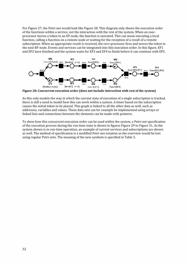
32  

 For Figure 27, the Petri‐net would look like Figure 28. This diagram only shows the execution order of the functions within a service, not the interaction with the rest of the system. When an exec‐processor moves a token to an EF‐node, the function is executed. This can mean executing a local function, calling a function on a remote node or waiting for the reception of a result of a remote subscription. When an appropriate result is received, the recv‐processor fires and moves the token to the next RF‐node. Events and services can be integrated into this execution order. In this figure, EF1 and EF2 have finished and the system waits for EF3 and EF4 to finish before it can continue with EF5.  

 Figure 28: Concurrent execution order (does not include interaction with rest of the system)  As this only models the way in which the current state of execution of a single subscription is tracked, there is still a need to model how this can work within a system. A timer based on the subscription causes the initial token to be placed. This graph is linked to all the other data as well, such as addresses, variables and values. These data sets can for example be implemented using arrays or linked lists and connections between the elements can be made with pointers.   To show how this concurrent execution order can be used within the system, a Petri‐net specification of the execution process during the run‐time state is shown in figures Figure 29 to Figure 31. As the system shown is in run‐time operation, an example of current services and subscriptions are shown as well. The method of specification is a modified Petri‐net notation as the overview would be lost using regular Petri‐nets. The meaning of the new symbols is specified in Table 3. 

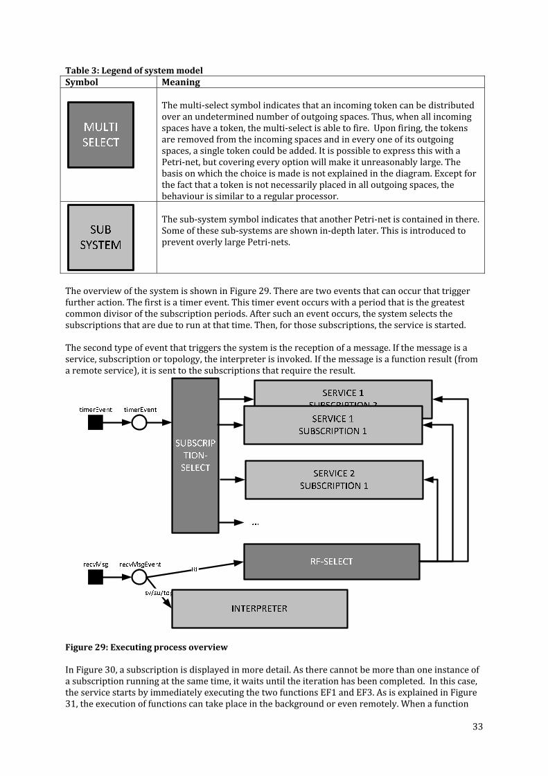
33  

Table 3: Legend of system model Symbol  Meaning  

  

 The multi‐select symbol indicates that an incoming token can be distributed over an undetermined number of outgoing spaces. Thus, when all incoming spaces have a token, the multi‐select is able to fire.  Upon firing, the tokens are removed from the incoming spaces and in every one of its outgoing spaces, a single token could be added. It is possible to express this with a Petri‐net, but covering every option will make it unreasonably large. The basis on which the choice is made is not explained in the diagram. Except for the fact that a token is not necessarily placed in all outgoing spaces, the behaviour is similar to a regular processor.  

 

 The sub‐system symbol indicates that another Petri‐net is contained in there. Some of these sub‐systems are shown in‐depth later. This is introduced to prevent overly large Petri‐nets. 

 The overview of the system is shown in Figure 29. There are two events that can occur that trigger further action. The first is a timer event. This timer event occurs with a period that is the greatest common divisor of the subscription periods. After such an event occurs, the system selects the subscriptions that are due to run at that time. Then, for those subscriptions, the service is started.   The second type of event that triggers the system is the reception of a message. If the message is a service, subscription or topology, the interpreter is invoked. If the message is a function result (from a remote service), it is sent to the subscriptions that require the result.  

 Figure 29: Executing process overview  In Figure 30, a subscription is displayed in more detail. As there cannot be more than one instance of a subscription running at the same time, it waits until the iteration has been completed.  In this case, the service starts by immediately executing the two functions EF1 and EF3. As is explained in Figure 31, the execution of functions can take place in the background or even remotely. When a function 

34  

result is received (either from local or remote execution), the execution can continue. Thus, when SV1 receives a token and the suInit‐space has a token, both EF1 and EF3 can be executed. This moves the tokens to the EF1 and EF3‐spaces. When, for example, EF1 finishes executing, it returns an RF‐message that results in a token in msgRF1. This allows the processor to fire, which results in a token in RF1. If, in the meanwhile, RF3 has not been received yet, EF2 can already be executed.  When the event trigger ET1 is encountered, the system bases its decision on whether to continue or abort the execution on the value of RF5.     

35  

 

 Figure 30: Subscription­part of the execution process  

36  

In Figure 31, the execution of a function (the exec‐processor from Figure 30) is examined. This is what occurs before a token is moved to an EF‐space in the previous figure.  If the EF is a remote subscription, then nothing needs to be executed at that time as the subscription is in place already (set during deployment) and the results will come in through a message event. When a function is called on a dynamic address, a message is sent that contains the call (by e.g. a temporary service). For local functions, the correct function is selected and its execution is deferred. After the execution has been completed, the result is returned through the RF‐select.  

execFunc execFunc

doNothing

Remote Static/ Static

FUNCTIONSELECT

Local

SEND MSG

Remote Dynamic

FN1

FN2

FN3

...

continue

e

continue

e

continue

e

FN1execFN2execFN3exec

execFN3 execFN2execFN1

RF‐SELECT

 Figure 31: Function execution part of the executing process (exec­processor in Figure 30)  On the basis of these models, an implementation can be created. The choices and selections used in the models are made using data on the services and subscriptions. Thus, a data structure needs to be created to hold this. It can be created on the basis of Figure 18. During the deployment phase, the data is entered into the structure through configuration instructions. In the run‐time phase, the system’s operation is equivalent with the movement of tokens in the models. A more detailed description of a prototype implementation that implements this system can be found in 6.1. It also describes the interaction with the data structure.  The disadvantages of this method, compared to a sequential bytecode interpreter, lie mostly in a more resource‐intensive execution process. The current prototype implementation has a relatively high complexity. However, when optimized, the execution should be much more efficient than currently. Hardware optimization may make it even more resource‐efficient than regular interpreters. Unfortunately, we cannot determine yet how much energy is lost or gained using this method.  This method of expressing concurrency makes it especially suited for an event‐based operating system such as TinyOS. That operating system uses split‐phase operations, in which the execution of 

37  

a function and reception of its result are separated. (37) This could be mapped onto the same operations in the Petri‐net.   Direct transfer of the graph representation instead of the postorder traversal‐representation of the parse tree is a possibility as well. There are some disadvantages to this however. The Petri‐net representation is intended to be as efficiently executable as possible and therefore will most likely contain optimizations that cannot be easily transferred. For example, direct pointers may be used or there can be reuse of addresses or values used in other services on the node. The configuration‐step, which occurs after the interpreter is invoked to process a new service, is used to effect these optimizations. Transferring this optimized representation directly is the intention in the deployment‐option in which nodes cannot add individual services. Transferring an unoptimized form of the graph‐like form to the nodes and maintaining the option to add individual services per node is an option as well. We did not research this option however.  In conclusion, the way of storing the executable form of the application on a node is a significant choice. Using an executing process that executes a concurrent application instead of sequentially interpreting instructions has advantages in the event‐oriented environment of WSN’s. However, due to more intensive processing per instruction, it is currently unknown whether this will result in less energy cost.   

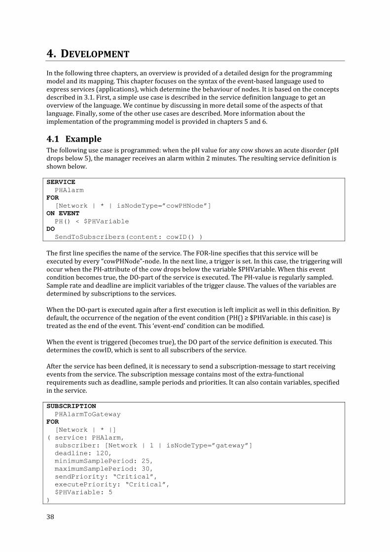
38  

4. DEVELOPMENT In the following three chapters, an overview is provided of a detailed design for the programming model and its mapping. This chapter focuses on the syntax of the event‐based language used to express services (applications), which determine the behaviour of nodes. It is based on the concepts described in 3.1. First, a simple use case is described in the service definition language to get an overview of the language. We continue by discussing in more detail some of the aspects of that language. Finally, some of the other use cases are described. More information about the implementation of the programming model is provided in chapters 5 and 6. 

4.1 Example The following use case is programmed: when the pH value for any cow shows an acute disorder (pH drops below 5), the manager receives an alarm within 2 minutes. The resulting service definition is shown below.  SERVICE PHAlarm FOR [Network | * | isNodeType=”cowPHNode”] ON EVENT PH() < $PHVariable DO SendToSubscribers(content: cowID() ) The first line specifies the name of the service. The FOR‐line specifies that this service will be executed by every “cowPHNode”‐node. In the next line, a trigger is set. In this case, the triggering will occur when the PH‐attribute of the cow drops below the variable $PHVariable. When this event condition becomes true, the DO‐part of the service is executed. The PH‐value is regularly sampled. Sample rate and deadline are implicit variables of the trigger clause. The values of the variables are determined by subscriptions to the services.  When the DO‐part is executed again after a first execution is left implicit as well in this definition. By default, the occurrence of the negation of the event condition (PH() ≥ $PHVariable. in this case) is treated as the end of the event. This ‘event‐end’ condition can be modified.  When the event is triggered (becomes true), the DO part of the service definition is executed. This determines the cowID, which is sent to all subscribers of the service.  After the service has been defined, it is necessary to send a subscription‐message to start receiving events from the service. The subscription message contains most of the extra‐functional requirements such as deadline, sample periods and priorities. It can also contain variables, specified in the service.  SUBSCRIPTION PHAlarmToGateway FOR [Network | * |] ( service: PHAlarm, subscriber: [Network | 1 | isNodeType=”gateway”] deadline: 120, minimumSamplePeriod: 25, maximumSamplePeriod: 30, sendPriority: “Critical”, executePriority: “Critical”, $PHVariable: 5 )

39  

Multiple subscriptions can be taken from one service. Besides stating which node subscribes to which service, the message specifies the extra‐functional properties shown in Table 4:  deadline:  The maximum amount of time that is allowed to pass between the 

generation of a message by the service and its reception by the destination. 

minimumSamplePeriod:  The minimum amount of time between two subsequent readings of the sensor values. 

maximumSamplePeriod:  The maximum amount of time between two subsequent readings of the sensor values. 

sendPriority:  The priority by which a message is sent over the network. executePriority:  The priority by which a service is executed. Table 4: Extra­functional properties in a subscription message  A mapping of this use case onto the WSN is shown in 5.2.3. 

4.2 General service definition structure The general structure of a service definition has the following format:  SERVICE

<Name> FOR

<Destination> ON EVENT

<Event Condition> DO

<Action> ON EVENTEND

<Event End Condition> DO

<Action>

4.2.1 Name The first parameter of a service definition is the service’s name. The name is a unique identifier for a service. It allows a developer to subscribe to that particular service using its name.  

4.2.2 Destination The second parameter, destination, determines on which nodes the service will run. The addressing takes place through a content‐based address, discussed more in‐depth in 4.3.   Another option would have been to not specify a destination, but let the WSN decide on the best nodes to run this application. This could be accomplished by determining the services and functions required in the event conditions and in the action‐part and using these to determine the nodes best suited for this task. As explained in 3.1, due to the difficulty with distributing tasks, we did not further pursue this option. 

4.2.3 Event condition 

The event condition contains a condition, which upon becoming true, triggers the action part. Responding to an event is often useful in WSN’s. Often this event is not a ‘real event’ as an event triggered by an interrupt, but is a change in values occurring after a reading of the sensors.   In this programming language, the event condition is in essence a Boolean function, which can consist of several sub‐functions. A future possibility is to add real events into it. 

40  

4.2.4 Event end condition Though we are interested in occurrences of events, we are detecting whether a certain condition is true at a certain time. The conversion from condition to event can take place by considering it an event only when the value of the condition becomes true. This means that the system will execute the action when the condition goes from false to true. The next event occurs when the condition goes from false to true again. However, one may want to perform an action when the condition goes from true to false as well. For this an event end action can be defined.  Defining only actions for when a single condition becomes either false or true is too simple for many relevant applications. For example, in a temperature‐monitoring application one can define that a message should be sent after the temperature becomes over 40 degrees. Using only an event condition temperature > 40, it would occur that a message would be sent when the temperature goes from 41 to 40 and back to 41. In many cases, a margin is desired for when the system considers it a new event. By defining an event end condition, one can set this. For example, by setting the event end condition to temperature < 39, the system would only send a new message after the temperature dropped below 39 and raised up to 41 again.  In effect, the state machine of the application is modified using the event end condition. While previously, it was as shown in Figure 32, it becomes like that as shown in Figure 33. In Figure 32, the event action is executed when the event condition becomes true. The event condition first has to become false before it can be executed again. The difference with Figure 33 occurs on the transition from when the system goes from the ‘event occurred’‐state to the ‘event not occurred’‐state. When the event end condition is specified, the trueness of this condition is considered instead of the falseness of the event condition.  

 Figure 32: State diagram when only an event condition is defined   

 Figure 33: State diagram for when both an event and an event end condition are defined   

4.2.5 Action The action‐part contains a function that is executed when the event is triggered. Functions are explained more in‐depth in 4.4. 

41  

4.3 Addressing of nodes As the network is not abstracted over in our approach, a method is needed to address them. As explained in 3.1.2, methods such as IP can be used to address the nodes, but from a service‐development point‐of‐view a semantically more meaningful method of addressing may be desired. In general, when one wants to address a node, one wants to address that nodes based on the properties that node has. For nodes, there are several attributes that could be considered interesting from a development‐point of view: functionality, sensor values, position and energy.  Addressing has the purpose of selecting a subset of nodes from a set of nodes. It is needed for cases in which only a subset of nodes needs to respond to certain information. This serves both a functional and a performance goal. It is functional in the sense that nodes may respond to the information in a way that does not conform to the desired functionality. The performance goal is served by preventing work to be carried out which is not required in the end (efficiency). Thus, any method of addressing should serve these goals.  We use a predicate‐like form of addressing. The predicate can be applied to a node to find out if it is part of the selection or not. In practice, a node does not always have to evaluate for itself whether the predicate is true for itself or not. 

4.3.1 Address notation In our programming model, the following notation for addressing nodes was chosen:  [ <Scope> | <Number> | <Properties> ] To address a node or a set of nodes, these three values have to be entered within the square bracket notation. For example: to address all nodes of the entire network which are of the type “CowNeckNode”, one would use the following notation:  [ Network | * | nodeType=”CowNeckNode” ]  To go more in‐depth into what constitutes an address in this language, first the scope is considered. 

Scope 

The scope indicates a subset of nodes of a network, previously defined based on logical and performance‐related characteristics. How exactly such subsets can be defined is explained in the chapter on clustering.   Examples of such clusters can be all sensors attached to a single cow or all sensors in a single house. For example, when a node attached to a cow wishes to address the temperature node sensor of the same cow, it can utilize the following notation:  [ Cow | 1 | nodeType=”CowTemperatureNode” ]

Number By addressing nodes in such a manner, it is possible for an address not to be unique. In some cases, it is meant to address all nodes which conform to the address. For example, when specifying that a certain alert service should run on all temperature nodes it is necessary to indicate that all selected nodes should perform the service. In other situations, only a single node which conforms to the address should be selected. This could occur when, for example, a room has multiple temperature sensors, but for energy efficiency a measurement from a single node is sufficient.  For many applications, the choice between selecting a single node and selecting all nodes conforming to the address is sufficient. In this language, it is noted in this manner:    

42  

 1 Select a single node conforming to the address specification. * Select all nodes conforming to the address specification. 

Properties The last part of addressing in this language has similarity to predicate logic. It is a conjunction of the comparison of properties to certain values the addressed nodes should satisfy. A property is a function that exists locally on a node. More on these functions is explained in 4.4.   The notation used for such a property is as follows:  <Property><Parameters> <Operator> <Value>  The <Value> in this address can indicate anything which delivers a value, namely a constant, local function or even a remote service.  To specify multiple properties within an address, the && is used to connect them. This occurs as follows:  <AddressProperty> && <AddressProperty>  Currently, the language only allows conjunction of properties. This is done for reasons of performance. Allowing disjunction as well as conjunction would make the processing of such an address significantly more complicated. Allowing disjunction instead of conjunction would be less feasible as most applications appear to require conjunction more.  As an example we address all temperature nodes located in the living room, which have a temperature of less than 20 degrees:  [Network | * | location=”LivingRoom” && Temperature < 20]

Possible additions The currently specified features cover only a part of the addressing functionality that can be desired for a WSN. For the applications that were considered for this language, these were considered to be the most important. There are some other properties which could be added into this notation to make it more complete.  One possible extension might be to make the number‐possibilities more thorough by allowing more possibilities than selecting either one or all nodes. Possibilities would include other absolute numbers or percentages.   Currently, the language allows for selecting one node out of several which satisfy the address. Often, this is used for utilizing a service on such a node. The language currently does not allow any specification on how that node is selected out of several which conform. It could be possible to allow specification of whether this selection should take place on the basis of hop‐distance, position‐distance, energy level or some sort of combination of these values, After specifying such a selection, it might even be specified after how long the selection should be re‐evaluated. 

4.3.2 Conclusion To make addressing within WSN’s feasible for programmers, important decisions should be easily implementable for programmers. In designing an address system, this should be considered as well as performance aspects.  

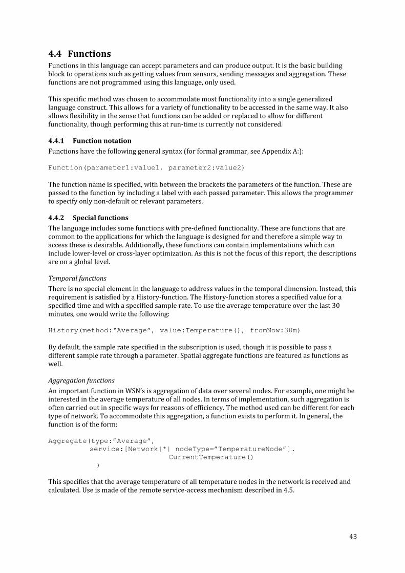
43  

4.4 Functions Functions in this language can accept parameters and can produce output. It is the basic building block to operations such as getting values from sensors, sending messages and aggregation. These functions are not programmed using this language, only used.   This specific method was chosen to accommodate most functionality into a single generalized language construct. This allows for a variety of functionality to be accessed in the same way. It also allows flexibility in the sense that functions can be added or replaced to allow for different functionality, though performing this at run‐time is currently not considered. 

4.4.1 Function notation Functions have the following general syntax (for formal grammar, see Appendix A:):  Function(parameter1:value1, parameter2:value2)  The function name is specified, with between the brackets the parameters of the function. These are passed to the function by including a label with each passed parameter. This allows the programmer to specify only non‐default or relevant parameters.  

4.4.2 Special functions The language includes some functions with pre‐defined functionality. These are functions that are common to the applications for which the language is designed for and therefore a simple way to access these is desirable. Additionally, these functions can contain implementations which can include lower‐level or cross‐layer optimization. As this is not the focus of this report, the descriptions are on a global level. 

Temporal functions There is no special element in the language to address values in the temporal dimension. Instead, this requirement is satisfied by a History‐function. The History‐function stores a specified value for a specified time and with a specified sample rate. To use the average temperature over the last 30 minutes, one would write the following:  History(method:“Average”, value:Temperature(), fromNow:30m)  By default, the sample rate specified in the subscription is used, though it is possible to pass a different sample rate through a parameter. Spatial aggregate functions are featured as functions as well. 

Aggregation functions An important function in WSN’s is aggregation of data over several nodes. For example, one might be interested in the average temperature of all nodes. In terms of implementation, such aggregation is often carried out in specific ways for reasons of efficiency. The method used can be different for each type of network. To accommodate this aggregation, a function exists to perform it. In general, the function is of the form:  Aggregate(type:”Average”,

service:[Network|*| nodeType=”TemperatureNode”]. CurrentTemperature()

) This specifies that the average temperature of all temperature nodes in the network is received and calculated. Use is made of the remote service‐access mechanism described in 4.5.  

44  

SendToSubscribers The common action to be taken after an event has been triggered is to send a message to the service’s subscribers. To accomplish this, the function SendToSubscribers is used. This function sends a value to the nodes that have subscribed to the service. The general form is:  SendToSubscribers(content:Temperature()) This specifies that the current temperature from the Temperature()‐function should be sent to the subscribers. 

4.4.3 Conclusion 

Functions are an abstraction used to accommodate a variety of core functionality of the system. These can only be accessed locally.  Currently, the language does not allow functions to return multiple values. In many situations, this can lead to difficulty. A possible solution would be to include support for tuples.   The access to aggregation‐functionality is rather troublesome. In the implementation, the “Aggregate”‐function should take care of gathering the values of the remote services and processing them in a way. This could be complicated and include the setting up of dynamic trees in the WSN.  

4.5 Remote services A key possibility in WSN’s is the ability to use the results from multiple nodes for a single application. This is supported in this language by allowing a service to use values produced by services running on other nodes. Such a remote service can be used in a similar way as local functions, but requires specification of the address and of subscription parameters. If subscription parameters are not entered, the service’s own subscription parameters are used.  

4.5.1 Remote service notation 

The general form of a remote service call is as follows:  <Address>.<ServiceName><SubscriptionParameters>  If, for example, one wishes to access a cow’s temperature service “Temperature” from a node in the same “Cow”‐cluster to obtain the current temperature of the cow, the desired subscription parameters should be determined. In this case, we consider that the non‐functional parameters can always be less stringent than the subscription parameters of the service itself. To enter this, we can specify it as follows:  [Cow|1|nodeType=”CowTemperatureNode”].Temperature( minimumSamplePeriod:

CurrentSubscription(param:“minimumSamplePeriod”)*2, maximumSamplePeriod:

CurrentSubscription(param:“maximumSamplePeriod”)*2, sendPriority: “Low” )  This indicates that the service should access a node within the “Cow”‐cluster which is of the type “CowTemperatureNode” to obtain the values produced by the Temperature service. Extra‐functionally, the sample period of the remote service can be double of that of the subscription of the local service and its “sendPriority” can always be “Low”. The “deadline” and “executePriority” are taken from the previous subscription by default. 

45  

4.5.2 Conclusion  The concept of ‘remote service calls’ is utilized to gain access to data from other nodes. A disadvantage of this method is that the coupling between several services can become quite great. An interesting advantage of this method is that the abstraction level allows for easy usability of this method; a remote service can intuitively be used where it is required.  Another possibility would be to communicate with other nodes on the level of ‘messages’ or ‘handlers’. This sacrifices abstraction for lower coupling.  This part of the language is also one where it becomes very important to take into account how the system will work in practice. The response to exceptions, such as communication failure, should be considered in this as well. 

4.6 Subscriptions A subscriber can take out a subscription on a service running on a node. This will enable the subscriber to receive messages generated by the service. This method, similar to the publish/subscribe‐mechanism, enables loose coupling between the subscriber‐ and the service‐node, an important feature in relatively unreliable WSN’s. 

4.6.1 Subscription notation A subscription is specified as follows:  SUBSCRIPTION <SubscriptionName> FOR <ServiceNodeAddress> ( <Parameter>: <Value> … )  The subscription has a unique name, used to remove it when necessary. The address to which the subscription should be delivered is specified after FOR. Subsequently, the following subscription parameters are defined:  Table 5: Subscription parameters Parameter  Description service  The name of the service that should be subscribed to. subscriber  The address of the node which should become a subscriber to this 

service. deadline  The maximum amount of time that is allowed to pass between the 

generation of a message by the service and its reception by the destination. 

minimumSamplePeriod  The minimum amount of time between two subsequent readings of the sensor values. 

maximumSamplePeriod  The maximum amount of time between two subsequent readings of the sensor values. 

sendPriority  The priority by which a message is sent over the network. executePriority  The priority by which a service is executed. $variable  Subscription variables are declared in service definitions. The value 

that the variable should become for this subscription can be set here. 

4.6.2 Conclusion Subscriptions are used to add flexibility into the programming model while keeping the resource usage low. An additional choice can be made in the deployment‐phase on whether to include this flexibility or not.  

46  

4.7 Clustering Energy‐conserving routing methods are one of the main challenges involving WSN’s. Determining an appropriate routing algorithm and parameters is infeasible without information about the WSN. The logical, application‐related aspect of the WSN forms a part of this. Thus, to save energy in routing, one could specify this information in the application layer itself. This would be a cross‐layer optimization which would decrease abstraction, but improve energy usage.   To mitigate the loss of abstraction, it would be preferable to use concepts which can both be used for routing and have logical function in the development of services. As explained in 3.1.2, an example of such a concept is that of a ‘cluster’ of nodes. The cluster includes nodes which have a strong logical relation to each other. In a service definition, this cluster may be used in a logical way to specify the scope of remote service access.   For performance‐purposes, the limited scope may be exploited to decrease communication. The cluster may contain nodes which can fulfil special roles in routing. A clusterhead, for example, can act as a central server for intra‐cluster communication and a gateway can be responsible for inter‐cluster communication. The role‐assignment could be based on specific properties of the nodes. For example, a relatively powerful node with an easily replaceable battery can be set as clusterhead, while weaker nodes only communicate directly with the clusterhead. 

4.7.1 Cluster notation Before a service is deployed, a topology for the network can be configured. This might be a default topology for all services, a topology configured only for a specific service (e.g. a tree structure for aggregation functions) or a topology set for a specific time (e.g. a star topology in a milking station) . Currently, we only discuss how to establish a single topology.   In the herd control scenario, a cluster topology is preferred in which all nodes attached to the same cow form a cluster. The node attached to the cow’s neck should always perform the function of clusterhead and gateway. To configure the network for this topology, the following command is issued:  TOPOLOGY CLUSTER CowCluster FOR

[Network|*|isNodeType=“cowNeckNode”] ( CLUSTERHEAD: [Network|*|isNodeType=“cowNeckNode” &&

cowID=<<cowID()>>], GATEWAY: CLUSTERHEAD, MEMBER: [Network|*|cowID=CLUSTERHEAD.cowID] )  This defines a topology of type CLUSTER, with the name “CowCluster”. CLUSTERHEAD, GATEWAY and MEMBER are parameters of this type CLUSTER. The CLUSTERHEAD is the node which receives and resends all intra‐cluster communication, the GATEWAY is responsible for inter‐cluster communication and MEMBER is a member of a cluster. These are all keywords of the language.   The meaning of this command is that a cluster’s clusterhead is the node located on the cow’s neck. For each clusterhead, the cluster’s gateway is the same as its clusterhead and its members are those nodes that have the same cowID as the clusterhead.  The square brackets are used to address nodes, based on their functions/attributes. In its first use (in the FOR), all nodes are addressed that have “cowNeckNode” as their “isNodeType”. The “isNodeType”‐attribute must be predefined on the nodes. The node currently executing the command is addressed as ‘node’. This results in the command being received by the neckstrap nodes. These nodes will further process the command to establish the cluster (including the non‐neckstrap nodes). The gateway is specified to be equivalent to the earlier specified clusterhead. For members, the nodes are addressed that have the same cowID as the clusterhead’s cowID.  

47  

 The operational details of this statement are left undiscussed. Currently, some more research is required in how to express other topologies. Research on description and self‐configuration of topologies in homogeneous WSN’s has been performed in (34). We are focusing more on configuring topologies in heterogeneous WSN’s based on node functionality.  

4.8 Conclusion The language was designed around the concepts discussed in 3.1. A potential way of improving the usability of the language is by providing a graphical user interface (like UML). This would increase the clarity of aspects of the language. 

   

48  

5. DEPLOYMENT After the development of the service in the macroprogramming language, the code goes through the deployment phase. Deployment is the process of getting developed code into a run‐time condition. This phase includes some trade‐offs that will be discussed.  As explained in 3.2, a major trade‐off that should be made in the deployment phase is that between resource usage and flexibility. The method of implementing this trade‐off is not discussed in detail. The primary difference between the options is whether a deployment step will be executed on the gateway or on nodes. Here, the focus is on the deployment option in which nodes run an interpreter that can receive new services.   This chapter discusses the various processes involved in the deployment. First, the translation from source code to bytecode is described and subsequently the translation of bytecode to a system that can be executed. 

5.1 Translation to bytecode Translating a program written in the macroprogramming language to bytecode involves several steps, namely: parsing code, translation to the stack‐based instruction language and a conversion of strings to compressed form.   A compiler for this language was created. Its grammar, an older version of the language, is shown in Appendix A:. 

5.2 Bytecode interpreter The bytecode interpreter converts bytecode into a form that can be easily executed by the node. In Figure 21, it is the step from configuration instructions to the configuration. This conversion takes place due to the necessity of bytecode being of small size and the executable form being executable with low use of system resources. It was considered that the translation phase can be relatively resource‐intensive, as it should not occur often in the lifetime of a node.  The interpreter which performs the translation is a stack‐based interpreter. The bytecode contains several “PUSH”‐instructions which push values onto the stack. The other instructions cause the interpreter to take values off the stack and place them into tables. There are, for example, tables for storing addresses, parameters and functions. Because the system is intended to work in an event‐based manner, the elements should quickly be random accessible. Processing the ‘linear’ bytecode before its execution and storing it in tables provide such a method. The tables will most likely be implemented as linked lists to accommodate variable sizes of services, subscriptions and their components.  The essential part of the table structure, which contains the order of execution of functions, is encoded as a graph as discussed in 3.3 The other tables serve to store specifics on what needs to be executed. 

5.2.1 Stack types The interpreter utilizes several stacks for processing the bytecode. Possibly they could be combined into a single stack, but this has not been considered. The stacks are:    

49  

 Table 6: Stacks used by bytecode interpreter Stack type  Use General stack (GS) 

The general stack contains the values that belong to PUSH‐instructions in the bytecode. 

Value stack (VS) 

The value stack contains a reference to the last value that has been processed and put in a table. This can be a either a constant or a function result. 

Execution stack (ES) 

The execution stack contains a reference to the last executed function. This is used to determine the order of execution. 

5.2.2 Execution tables After the bytecode has been interpreted, its interpreted contents will be placed into the execution tables. At the core of the structure is the execution order, as explained in 3.3. Around it are the various concepts described in 3.1.    The structure of these tables is displayed in Figure 34.  

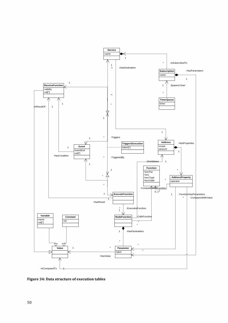
50  

-validity-val[*]

ReceiveFunction

ExecuteFunction

NodeFunction

-token[*]TriggersExecution

* -TriggeredBy

* -Triggers

-ExecutesFunction*1

-HasResult

1

-IsResultOf 1

-labelParameter

-valConstant

-name-val[*]

Variable

-eventEnd-val[*]

Event

-nameService

1

1

-scope-amount

Address

-operatorAddressProperty

-nameSubscription

-timerTimerQueue

-HasCondition

1

1

-HasDestination1

1

-HasProperties

1

*

-HasParameters1

*

1

-IsSubscribedTo*

-SpawnsTimer1

*

-HasParamaters

1

*

-FunctionHasParameters1

*Value

-HasValue

*1

-ComparesWithValue*

-IsComparedTo 1

-funcPar-func-funcType-funcValid

Function

-CallsFunction

*

0..1-ComparesWithFunction

*

1

*

1

*

1

1

*

*

-OnAddress 1

*

1

*

1

  Figure 34: Data structure of execution tables    

51  

Below, the use of these tables is explained. For each variable of a table, the ‘refers’‐column indicates whether it the variable points to another table. If multiple tables are mentioned, the variable can refer to one of these. 

Service (SV) The SV‐table contains the services running on the node. The name is stored along with the original destination address. It is connected to the TE‐table to trigger the first functions to be executed of a service.  Variable  Refers  Use name    The name of the service. address  AD  A reference to the address  

Receive Function (RF) The RF‐table contains reception of function results. For each function call, there is an RF‐entry. This reception can be from a local function as well as a remote service. It corresponds to the RF described in 3.3.  Variable  Refers  Use execfunc  EF  Is function result from this function. validity    Indicates if the function result is: 

• Constant: Function result never changes (e.g. an identifier). • Dynamic: Function result can change every time the function is called.• Dependent: Function result can only change if the parameter values of 

the function change. Used for reducing the number of function calls as much as possible (as they can be remote). 

val[]    Stores the latest result. Value is stored per subscription. 

Execute Function (EF) The EF‐table contains pointers to the actual function calls. This table is linked with RF through TE to form a graph to determine execution order. It corresponds to the EF described in 3.3.  Variable  Refers  Use func  NF  Points to the function call with its parameters. recvfunc  RF  Result of the function will be sent there. 

Triggers Execution (TE) The TE‐table contains the connections between the reception of a function result and the execution of the next. In essence, it contains the order of execution as it specifies which functions should have been executed before a certain function will be executed. Together with EF and RF forms a Petri‐net as shown in Figure 28.  Variable  Refers  Use recvtype    recvfunc points to either a service, an event or a function. recvfunc  RF,ET,SV A reception of a result here triggers the execution of execfunc. exectype    execfunc points to either an event or a function. execfunc  EF, ET  This is executed after recvfunc has been received. token[]    Set to true if a result has been received at recvfunc. Set to false after the 

execfunc has been executed. Value is stored per subscription. 

Node Function (NF) The NF‐table contains the actual function calls with their parameters. It points to the function that should be called and the parameters that should be passed. 

52  

 Variable  Refers  Use address  AD  The address on which the node should be executed (if remote). func  FN  The function that should be executed. params  PA  The parameters that should be passed. nrparams    The number of parameters that should be passed. 

Parameter (PA) The PA‐table contains the parameters of an NF, AP or SU‐entry. These contain the label of the parameter along with a pointer to a value, which can be a pointer to an RF‐entry, a variable, or a constant.  Variable  Refers  Use label    Label of parameter. constant    Whether val is a function, a constant or a variable. val  RF,CO,VAR Points to the parameter value. 

Function (FN) The FN‐table contains the functions located on the node along with information on their validity. This indicates whether the function result is always the same (static), always changing (dynamic) or dependent on the parameters (dependent). It also indicates its return type. In the current implementation, data on the parameters of the function are stored here as well.  Variable  Refers  Use funcpar    Whether the entry is a function or a function parameter. func    The name of the function. functype    The type of the function: void, int, string or Bool.  funcvalid    Indicates if the function’s result is: 

• Constant: Function result never changes (e.g. an identifier). • Dynamic: Function result can change every time the function is 

called. • Dependent: Function result can only change if the parameter values 

of the function change. Used for reducing the number of function calls as much as possible (as they can be remote). 

Constant (CO) The CO‐table contains the constants that are used in services.  Variable  Refers  Use val    Value of the constant. 

Variable (VAR) The VAR‐table contains the variables that are specified through subscriptions.  Variable  Refers  Use name    Name of the variable. val[]    Contains the value of the variable. Value is stored per subscription. 

Address (AD) The AD‐table contains the addresses used in services and subscriptions. An entry includes the scope and the amount and references the AP‐table for its address properties.    

53  

 Variable  Refers  Use scope    The scope of the address. amount    The amount of the address. props  AP  The properties of the address. nrprops    The number of properties of the address. 

Address Property (AP) The AP‐table contains address properties belong to an address. It references a local function, an operator to use for comparing and a value to compare the function with.  Variable  Refers  Use func  FN  Points to the local function. funcpar  PA  Points to the parameters that are passed to that function. funcparnr    The number of parameters passed. op    The operator used for comparison. constant    Whether val is a function, a constant or a variable. val  RF,CO,VAR  Points to the value for comparison. 

Event Trigger (ET) The ET‐table contains the events and the eventends specified in services. It contains indication on whether it is an event or an event end, an evaluated condition (true or false) per subscription and references the RF‐table for its condition.  Variable  Refers  Use ee    Whether the event is an event condition or an event‐end condition. trigger  RF  The event condition. val[]    The evaluated condition value. Value is stored per subscription. 

Subscription (SU) 

The SU‐table contains subscriptions belonging to a service. For its parameters it references the PA‐table.  Variable  Refers  Use name    Name of the subscription. service  SV  Is a subscription to this service. params  PA  The subscription parameters. nrparams    Number of subscription parameters. 

Timer Queue (TQ) The TQ‐table contains the various timers that come into existence due to the subscriptions. It is used to start the appropriate services at the appropriate times.   Variable  Refers  Use su  SU  Belongs to this subscription. timer    Its period.  

5.2.3 Processing bytecode The bytecode interpreter translates the bytecode to the previously defined tables using the stacks. It is the process that forms the service and subscription Petri‐nets as shown in Figure 30. To describe this process, we use pseudo‐code to prevent getting in too much detail. Per instruction, we indicate the operations that occur on the stacks and tables when this instruction is interpreted. For example:  

54  

VAR: Add <Val>, Receive <VARPtr>  This indicates that the value <Val> is added to the Variable‐table and a pointer its entry in the table is returned as <VarPtr>. Other operations than Push, Pull, Add and Receive may be used, but will be explained afterwards. 

Processing constants and variables 

Instruction  Stack & Table Behaviour PUSH <Val>  GS: Push <Val> CONSTANT  GS: Pull <Val> 

CO: Add <Val>, Receive <COPtr> VS: Push <COPtr> 

VARIABLE  GS: Pull <Val> VAR: Add <Val>, Receive <VARPtr> VS: Push <VARPtr> 

Algorithm 1: Processing constants and variables  The CONSTANT and VARIABLE instructions operate by pulling the value from the General Stack and adding it to the respective tables. Subsequently, a reference to the table entry is pushed onto the Value Stack. 

Processing functions Functions and remote service calls constitute the core of the execution pattern. To appropriately facilitate this, the functions from bytecode need to be converted into the Petri‐net‐like form that appropriately expresses both the order of execution and the event‐based way of operation.   The table below specifies the actions with respect to the stacks and tables the interpreter should take when encountering an instruction:  Instruction  Stack & Table Behaviour FUNCTION  GS: Pull <Function> 

GS: Pull <NrParams> For every parameter (<NrParams>): 

GS: Pull <ParamName> VS: Pull <ParamVal> PA: Add <ParamName>, <ParamVal>, Receive <PAPtr> If ParamVal is a function: 

ES: Pull <ParamRFPtr> TE: AddRF <ParamRFPtr> 

NF: Add <Function>, <PAPtr>, <NrParams>, Receive <NFPtr> EF: Add <NFPtr>, Receive <EFPtr> RF: Add <NFPtr>, Receive <RFPtr> TE: AddEF <EFPtr> ES: Push <RFPtr> If none of the <ParamVal>’s was a function: 

TE: AddPhase <EFPtr>, <CurrPhase> If FU:getFuncType(<Function>) indicates a return of value: 

VS: Push <EFPtr>  

Algorithm 2: Processing functions  The FUNCTION instruction causes the function name and the number of parameters to be pulled from the stack. Subsequently, each parameter will be read. First, the label of the parameter is pulled from the general stack. This is followed by pulling of the parameter value from the value stack. This value can be a constant, variable or other function. The parameters are placed in the PA‐table. If the 

55  

value was a function, it has to be executed before the present function can be executed. For this purpose, a reference to the RF will be put into the TE‐table.  Subsequently, the function with a reference to the parameters will be stored in the NF‐table. RF‐ en EF‐entries are created for the present function. To place the function into the order of operation, the EF‐entry is linked into the TE‐table. In practical terms, this means that the previously added references to the RF’s will be linked with the current function. This implies that any functions in the present function’s parameter need to have finished executing before the present function can continue.  However, when the function does not depend on any other function it should be executed as well. To accomplish this, either the service entry or the event entry is set to trigger the function, depending on the place where the function occurs. If the function returns a type (this is looked up in the FN‐table), a reference to the function’s RF is pushed onto the Value Stack.  Instruction  Stack & Table Behaviour REMOTEFUNCTION  GS: Pull <Address> 

GS: Pull <Service> RS: Add <Address>, <Service>, Receive <RemoteServicePtr> GS: Pull <NrParams> For every parameter (<NrParams>): 

GS: Pull <ParamName> VS: Pull <ParamVal> PA: Add <ParamName>, <ParamVal>, Receive <PAPtr> If ParamVal is a function: 

ES: Pull <ParamRFPtr> TE: AddRF <ParamRFPtr> 

NF: Add <RemoteServicePtr>, <PAPtr>, <NrParams>, Receive <NFPtr> EF: Add <NFPtr>, Receive <EFPtr> RF: Add <NFPtr>, Receive <RFPtr> TE: AddEF <EFPtr> ES: Push <RFPtr> If none of the <ParamVal>’s was a function: 

TE: AddPhase <EFPtr>, <CurrPhase> If FU:getFuncType(<Function>) indicates a return of value: 

VS: Push <EFPtr>  

Algorithm 3: Processing remote functions  The interpretation of the REMOTEFUNCTION‐instruction is similar to that of the FUNCTION‐instruction. It differs in the sense that first the address reference is pulled from the General Stack and an entry is created in the RemoteService‐table. 

Processing addresses Below we describe the interpretation of the ADDRESS‐instruction.  Instruction  Stack & Table Behaviour ADDRESS  GS: Pull <Scope> 

GS: Pull <Amount> GS: Pull <NrProps> For every property (<NrProps>): 

GS: Pull <Function> GS: Pull <NrParams> For every parameter (<NrParams>): 

GS: Pull <ParamName> 

56  

VS: Pull <ParamVal> PA: Add <ParamName>, <ParamVal>, Receive <PAPtr> 

GS: Pull <Operator> GS: Pull <NrOpParams> VS: Pull <Value> AP: Add <Function>, <PAPtr>, <Operator>, <Value>,  

Receive <APPtr>  AD: Add <Scope>, <Amount>, <APPtr>, Receive <ADPtr> GS: Push <ADPtr>  

Algorithm 4: Processing addresses  The ADDRESS instruction pulls the scope and amount of the general stack. Subsequently, it will start to read the properties of the address. It starts by reading the amount of properties that it should read, then for each property the function which will be compared along with its parameters, the operator which does the comparison and the value it is compared to. Afterwards these are entered into the address properties (AP) and address (AD) tables. As an optimization, the AD and AP‐tables can be checked to see if the same address already occurs in the table; if it occurs, a pointer to the existing address is returned. 

Processing other instructions 

Other instructions shall not be covered in‐depth.  

Example To provide an idea about how such a service will be represented in the run‐time memory of a node, an example shall be provided. Below we specify the service that shall run on the nodes:  SERVICE TemperaturePHAlert FOR [Network|*|nodeType=”CowTemperatureNode”] ON EVENT (Temperature() > $MaxTemperatureAlert) && [Cow|1|nodeType=”CowPHNode”].PH($MaxPH: $MaxPHAlert) DO SendToSubscribers(content: cowID())  The compiler will translate this to bytecode. Bytecode will be in binary form, with strings in compressed form, but is represented here in a readable format.  PUSH “TemperaturePHAlert” SERVICE PUSH “CowTemperatureNode” CONSTANT PUSH 2 PUSH “=” PUSH 0 PUSH “nodeType” PUSH 1 PUSH “*” PUSH “Network” ADDRESS FOR

57  

PUSH 0 PUSH “Temperature” FUNCTION PUSH “one” PUSH “$MaxTemperatureAlert” VARIABLE PUSH “two” PUSH 2 PUSH “>” FUNCTION PUSH “one” PUSH “$MaxPHAlert” VARIABLE PUSH “$MaxPH” PUSH 1 PUSH “PH” PUSH “CowPHNode” CONSTANT PUSH 2 PUSH “=” PUSH 0 PUSH “nodeType” PUSH 1 PUSH 1 PUSH “Cow” ADDRESS REMOTEFUNCTION PUSH “two” PUSH 2 PUSH “&&” FUNCTION ONEVENT PUSH 0 PUSH “cowID” FUNCTION PUSH “content” PUSH 1 PUSH “SendToSubscribers” FUNCTION DO END Processing this bytecode will lead to the following entries contained in the execution tables. These may be implemented using arrays or linked lists. A reference to another entry is indicated by the letters of the table followed by the ‘index’ number of the entry. Constants are indicated in capital letters and strings will be in compressed form in the implementation.    

58  

 SV  Name 1  “TemperatureAlert”  FN  Name  Validity  ReturnType 1  “>”  DEPENDENT  BOOL 2  “&&”  DEPENDENT  BOOL 3  nodeType  STATIC  INT 4  cowID  STATIC  INT 5  SendToSubscribers  STATIC  NONE 6  Temperature  DYNAMIC  INT  CO  Value 1  “CowTemperatureNode” 2  “CowPHNode”  VAR  Name  Value[0]  Value[1]  Value[…] 1  $MaxTemperatureAlert       2  $MaxPHAlert        NF  Address  Function  Parameter 1  NULL  FN6  NULL 2  NULL  FN1  PA1 3    “PH”  PA3 4  NULL  FN2  PA4 5  NULL  FN4  NULL 6  NULL  FN5  PA6  PA  Label  Value 1  “two”  VAR1 2  “one”  RF1 3  “$MaxPH”  VAR2 4  “two”  RF3 5  “one”  RF2 6  “content”    EF  NodeFunction  ReceiveFunction 1  NF1  RF1 2  NF2  RF2 3  NF3  RF3 4  NF4  RF4 5  NF5  RF5 6  NF6  NULL  RF  Validity  Value[0]  Value[1]  Value[…] 1  DYNAMIC       2  DEPENDENT       3  DYNAMIC       4  DEPENDENT       5  STATIC           

59  

 TE  Receive  Triggers  Token[0]  Token[1]  Token[…] 1  SV1  EF1       2  RF1  EF2       3  SV1  EF3       4  RF3  EF4       5  RF2  EF4       6  RF4  ET1       7  ET1  EF5       8  RF5  EF6        ET  Condition  EventEnd  Value[0]  Value[1]  Value[…] 1  RF4  FALSE        AD  Scope  Amount  Properties 1  “Network”  *   2  “Cow”  1    AP  Function  Parameters  Operator  Value 1  FN3  NULL  “=”  CO1 2  FN3  NULL  “=”  CO2  This table still requires a subscription to finally run. The actual execution of these tables is discussed in chapter 6.  

5.3 Conclusion This chapter provided further detail on the deployment discussed in 3.2, with focus on the bytecode interpreter. The description is based on a prototype x86‐implementation that performs the translation to bytecode and the interpretation of bytecode, which ascertains the functional correctness. Further improvements can be made by increasing the efficiency of the execution tables. Possibilities for accomplishing this include sorting and generalizing the current tables.  

   

60  

6. RUN­TIME The run‐time phase is the phase in which the WSN performs the assigned tasks. This occurs after the deployment has been completed. The approach discussed in 3.3 is described in terms of algorithms that use the execution tables from 5.2. 

6.1 Execution method The Interpreter‐process has been described in 5.2. Discussion of the handling of incoming and outgoing messages will not be discussed in this report. For this paragraph, the focus will be on the Execution‐process.  The Execution‐process reads the tables produced by the Interpreter‐process as described previously in 5.2.3.  Its operation is described below. It should be noted that these algorithms are based on a prototype implementation and are not optimized.  For ease of understanding, the notation of the algorithm has been converted to pseudo‐code. A short explanation of the notation is shown in Table 7.   Table 7: Pseudo­code notation Notation  Meaning te ε TE  te is an entry from the “Triggers Execution”‐table.  In C‐code, this would be 

represented as: te_table[te]. The abbreviations for the tables and their content can be looked up in 5.2.2. 

For all te ε TE:  Iterate through all entries of TE. te.recvtype  The variable ‘recvtype’ of the entry te.  RF[te.recvfunc]  The entry of the RF table which is referred to by te.recvfunc. 

6.1.1 Initiate service The general program loop is executed after a timer‐event. It generates the timerEvent from Figure 29.  Function  Behaviour Run()  /* time is a variable which expresses the current time as a value between 0

and the least common multiple of all subscription times. This function is called on a timer event which occurs on the greatest common divider of all subscription times. */

 For all tq ε TQ: 

If (time % tq.timer == 0) For all te ε TE: 

If (te.recvtype == SV &&      te.recvfunc == SU[tq.su].service): 

te.token[tq.su] = TRUE;  For all su ε SU: 

performStep(su); Algorithm 5: General execution loop  The algorithm determines if it is time for a subscription to a service to be scheduled for execution by checking the TQ‐table against the timer. If it is, the TE‐table will be searched to find the first functions which should be executed of the subscription’s service. These occurrences will be marked by setting its token to TRUE.   Subsequently, an iteration step is performed for each subscription.  

61  

6.1.2 Iteration step In the iteration step, the channels from Figure 30 are checked for tokens and the appropriate processors are fired. This step proceeds as follows:  Function  Behaviour performStep(su)  For all ef ε EF: 

tokens = TRUE token_occurs = FALSE  /* If EF has an incoming RF without a token, do not execute the EF (tokens = FALSE) */

For all te ε TE: If (te.exectype == EF && ef == te.execfunc): 

token_occurs = TRUE  If (te.token[su] == FALSE): 

tokens = FALSE  

/* If all the EF's incoming RFs have a token, execute the EF */ If (tokens && token_occurs): 

execEF(ef, su)  /* Remove tokens from the EF */ For all te ε TE: 

If (te.exectype == EF && ef == te.execfunc): te.token[su] = FALSE  

/* For every ET-entry, see whether the condition holds. If yes, execute the DO. If no, do not continue.*/ For all et ε ET: 

For all te ε TE: If (te.exectype == ET && ef == te.execfunc &&  

te.token[su]): /* Remove token and place result value in ET-value */ te.token[su] = FALSE /* If the event condition was not previously the same as now, continue */

val = RF[te.recvfunc].val[su]] If (et.val[su] != val): 

et.val[su] = val /* If the event condition is true, place tokens in the execution tables */ If (val): 

/* Place tokens in upcoming places */ For all te2 ε TE: 

If (te2.recvtype == ET &&  te2.recvfunc == et): te2.token[su] = TRUE 

Algorithm 6: Execution iteration step  This iteration step is responsible for executing the functions which should be executed and for updating the tokens. It accomplishes this by checking for all EF’s whether all required tokens for it to execute are there in the TE‐table. If so, the function is executed. After execution, the tokens are removed.  Besides executing the relevant EF’s, the Event Triggers are evaluated as well. To accomplish this, for all ET’s the RF‐table is checked on whether its condition has been evaluated to TRUE or FALSE.  As 

62  

this is about events, not just conditions, it will only proceed by placing tokens at upcoming functions when the condition is currently TRUE while it was previously FALSE.  This algorithm could be optimized by sorting the tables beforehand. Currently, the complexity is O( EF * (TE + nrTokens(O(execEF) + TE)) + ET * (TE * nrTokens(TE)) ). The nrTokens is the number of TE‐entries which have a token. Its complexity can be greatly reduced by sorting the TE table by EF and ET. This at minimum eliminates the need for the EF and ET terms. As this is essentially an algorithm for an uncoloured Petri‐net, better performance can most likely be achieved by looking at efficient algorithms for Petri‐nets, but this will not be studied in this report. 

6.1.3 Receive function result To execute an EF, as shown in Figure 31, the following function is called:  Function  Behaviour execEF(ef, su)  nf = ef.func 

 /* Case distinction on address */

If (not( isRemote(ef) )): val = execFunc(nf.func, nf.params, nf.nrparams, su)  /* If the return type of the function is not void, place the result in its RF */

If (getFuncType(nf.func != VOID)): recvRF(ef.recvfunc, su, val) 

 Algorithm 7: EF execution  The “execEF”‐function is responsible for executing the required EF. It first determines if the function is local, then executes the function and passes along its parameters. Subsequently, if the function has a return‐value, this value is sent to “recvRF”.  Function  Behaviour recvRF(rf, su, val) 

/* Place the received value in the RF table */ rf.val[su] = val  /* Place tokens in TE where this RF occurs */

For all te ε TE: If (te.recvtype == RF && te.recvfunc == rf): 

/* Placing token */ te.token[su] = TRUE 

 Algorithm 8: Receiving a function result  The “recvRF”‐function is responsible for receiving a value returned by a function and placing it in the right place in the RF‐table. Subsequently, tokens are added in the TE‐table on places where the RF triggers another function. Currently, its complexity is O(TE). 

6.2 Conclusion This chapter provided a more detailed description of the run‐time process discussed globally in 3.2.  The algorithm was provided to gain a better understanding on how the execution‐process works. The description is based on a functional x86‐prototype. However, the efficiency of the current version can be vastly improved.     

63  

7. EXAMPLE To show how the programming model can be applied, we describe an example. 

7.1 Cow scenario One of the use cases for WASP is using a WSN for monitoring the health of a herd of cows. This example will expand upon this idea.  

7.1.1 Setting The environment that the WSN will operate in is a dairy farm in the Netherlands. It has 200 cows, which is larger than the national average of 70(38), but not yet a so‐called ‘mega‐farm’. The farm is a family company run mostly by one person. The number of cows and the number of farmers necessitate automation of the farming process. The farm currently has the following elements: 

• A pasture with grass on which the cows can graze • A barn that houses the cows at night and that contains the milking machine • A house where the farmer lives • A farmer that operates the farm • A herd of 200 cows that graze and provide milk 

 This is displayed in Figure 35. 

 Figure 35: Overview of the farm   In the last few years, livestock health has increasingly been receiving attention. Mad cow disease, foot‐and‐mouth disease and blue tongue are just a few of the diseases that were featured prominently in the media. To more effectively monitor the health of his herd, the farmer wants to use a WSN. This data should be used both for registration, such that the farmer can observe long‐term patterns and for alerts, such that the farmer can respond quickly to a cow becoming ill. The most important data required for this are a cow’s temperature, stomach pH‐level and leg movement patterns. 

7.1.2 Nodes 

To fulfil these needs, the following sensor nodes will be attached to the cow: 1. A cow temperature node will be attached in the ear to measure the cow’s temperature 2. A pH node will be planted in the cow’s stomach to measure its pH‐level 3. An acceleration node will be attached to a cow’s leg to detect anomalies in its movement 4. A position node will be attached to a cow’s neck to determine its position 

64  

 Additionally, the barn will contain the following nodes: 

5. Barn temperature nodes are placed in the barn to measure its temperature 6. Barn luminosity nodes are placed in the barn to measure its light level 

 Furthermore, the farm contains a station for relaying information to the gateway.  As each node will be used differently, there are different hardware requirements for each node. The cow temperature node will be placed in‐ear. Most likely it needs to be rather small. It will be possible to recharge it, but not easily. As the pH‐sensor is placed in the stomach, its battery can not be replaced. Thus, a very long lifetime is required for it. Therefore, different types of node are used in the WSN.  These requirements are as follows:  Table 8: Size and lifetime requirements for cow nodes   Size  Lifetime Cow temperature  ‐  0 pH  ‐  ++ Acceleration  ‐  ‐ Position  +  ‐  The capabilities of these nodes must be available as functions. These are programmed at a lower level and made available to the interpreter for a node. These functions are:  Table 9: Specific functions available on the nodes Function  Parameter  Description Temperature    Returns the current temperature. 

Unit  The unit of the temperature value. Either: • “Celsius” (default) • “Kelvin” • “Fahrenheit” 

pH    Returns the current pH‐level Position    Returns the current position. Luminosity    Returns the current luminosity. Crippleness    Returns the degree to which the cow’s movement 

appears to be crippled. Is calculated by applying a complex algorithm over acceleration data for a specified period of time. Returns an integer between 0 (heavily crippled movement) and 100 (very normal movement). 

SampleTime  The time in ms during which the acceleration is sampled and the algorithm is applied. Greater values result in greater accuracy and energy usage. 

SetLight    Turns the light attached the node on or off. Level  Either: 

• “Off” • “On” • “Toggle” (default) 

cowID    Gets or sets a ‘cowID’‐value that identifies to which cow the node belongs. 

Action  Whether to write or read the ID: • “Get” (default) • “Set” 

65  

ID  When writing an ID, the integer value that should be set. 

 Table 10 shows the mapping of these functions to the nodes. Additionally, default functions such as “isNodeType” and “History” are present on the nodes.  Table 10: Mapping of functions to nodes Node  Contains cowTempNode  • cowID 

• Temperature cowPHNode  • cowID 

• pH cowAccelNode  • cowID 

• Crippleness cowPosNode  • cowID 

• Position barnTempNode  • Temperature barnLightNode  • Luminosity 

• SetLight 

7.1.3 Development After the capabilities of the nodes have been determined, the services can be written. Each use case should result in a service. To ease development, we start by defining a cluster topology on the network. As the position node will be the most powerful node on a cow, it will be made clusterhead. To be able to group the nodes per cow, the cowID will be used.  Use case  Set cluster topology for a cow Code  TOPOLOGY CLUSTER Cow

FOR [Network|*|isNodeType=“cowPosNode”] ( CLUSTERHEAD: [Network|*|isNodeType=“cowPosNode” && cowID=<<cowID>>], GATEWAY: CLUSTERHEAD, MEMBER: [Network|*|cowID=CLUSTERHEAD.cowID()] )

 Subsequently, the following services are defined:  Use case  Receive a regular report on the cows’ temperatures Code  SERVICE

TempReport FOR [Network | * | isNodeType=”cowTempNode”] DO SendToSubscribers(content: Temperature() )

 Use case  Receive an alert when the temperature of a cow crosses a certain temperature Code  SERVICE

TempAlert FOR [Network | * | isNodeType=”cowTempNode”] ON EVENT Temperature() > $TempVar DO

66  

SendToSubscribers(content:[Cow|1|isNodeType=”cowPosNode].Pos())

 Use case  Receive an alert when both the temperature and the pH of a cow cross certain values Code  SERVICE

TempPHAlert FOR [Network | * | isNodeType=”cowTempNode”] ON EVENT Temperature() > $TempVar && [Cow | 1 | isNodeType=”cowPHNode”].PH() < $PHVar DO SendToSubscribers(content: cowID() )

 Use case  Receive an alert when a cow appears to be crippled by detecting if the average of 

crippleness values over a period of time crosses a threshold Code  SERVICE

CrippleAlert FOR [Network | * | isNodeType=”cowAccelNode”] ON EVENT History(method:”Average”, value:Crippleness(SampleTime: $CrippleSampleTime), fromNow:$AvgTime) > $CrippleVar DO SendToSubscribers(content: cowID() )

 Use case  Turn on the light in the barn when the light drops below a certain level and turn it off 

when the light rises above a certain level Code  SERVICE

LightSwitch FOR [Network | 1 | isNodeType=”barnLightNode”] ON EVENT Average(func: [Network | * | isNodeType=”barnLightNode”].Luminosity() ) < $LightOnLuminosity DO SetLight(Level:”On”) ON EVENTEND Average(func: [Network | * | isNodeType=”barnLightNode”].Luminosity() ) > $LightOffLuminosity DO SetLight(Level:”Off”)

 As discussed in 3.1 and 4, a variety of extensions of the language is possible. Especially the addressing can be improved by selecting nodes not only by cluster, but also by physical‐ and hop distance. When these language concepts are introduced, services such as the following become possible:  Use case  Send an alert when there is no other cow within a 50m distance of a certain cow Code  SERVICE

LonelyCow FOR [Network | * | isNodeType=”cowPosNode”]

67  

ON EVENT Exist(node:[Distance(50) | * | isNodeType=”cowPosNode”]) = FALSE DO SendToSubscriber(content: cowID() )

 Use case  Turn on the light in the barn when the light drops below a certain level and there is a cow 

near or in the barn and turn it off when the light rises above a certain level or there is no cow nearby 

Code  SERVICE LightSwitchProximity FOR [Network | 1 | isNodeType=”barnLightNode”] ON EVENT Average(func: [Network | * | isNodeType=”barnLightNode”].Luminosity() ) < $LightOnLuminosity && Exists(node:[Hop(1) | 1 | isNodeType=”cowNeckNode”]) = TRUE DO SetLight(Level:”On”) ON EVENTEND Average(func: [Network | * | isNodeType=”barnLightNode”].Luminosity() ) > $LightOffLuminosity || Exists(node:[Hop(1) | 1 | isNodeType=”cowNeckNode”]) = FALSE DO SetLight(Level:”Off”)

7.1.4 Deployment As the farmer wants to be able to install new services on the nodes, he chooses the deployment‐option in which there is a bytecode‐interpreter on the nodes. The farmer buys the appropriate nodes that have the interpreter installed on them. Then, the system can be deployed by first setting a cowID on each sensor. This could be accomplished by holding a node close to a short‐range transmitter that sends the command. Subsequently, the nodes can be attached to the cows. From that point onwards, the nodes can be completely controlled remotely. The farmer then uses the graphical user interface on the gateway system to install the desired services and to configure subscriptions. 

7.2 Conclusion A description was given on how to apply the programming model to a specific case. With existing programming models, implementing the use cases would be much more difficult. The more abstract, node‐independent models cannot be applied to this heterogeneous WSN. If such a way of programming is required, all nodes need to be made similar, resulting in many difficulties. The only option left is to use the lower‐level programming models. This, however, will make programming more complex. The programmer would directly have to take care of aspects such as communication, configurability, reprogrammability, standard functions, and distribution of the application over the nodes. This can be simplified by re‐use of existing libraries and middlewares, but the integration of these would then be difficult. The programming model described in this thesis simplifies many of these aspects.      

   

68  

8. CONCLUSION The goal of this report was to describe a programming model for heterogeneous wireless sensor networks that addresses the needs for long lifetime, low cost, easy deployability, flexibility and robustness. The model also addresses the gaps existing in the current state‐of‐the‐art WSN programming models. A design‐based, constructive approach was taken to make decisions for the development, deployment and run‐time phases of the system.   Contributions The programming model simplifies the development of applications for heterogeneous WSN’s in particular, without greatly increasing energy usage. Existing programming models that provide high abstraction require homogeneous WSN’s, thus automatically excluding the advantages that heterogeneous WSN’s offer. The only other option is to use lower‐level programming models in which the programmer directly needs to spend significant effort on aspects such as communication, reprogrammability, and standard functions. Our programming model provides low‐effort control over such aspects.  For the development phase, a network‐centric, node‐dependent programming language was created. Contrary to current programming models, it is specifically designed to support heterogeneous WSN’s.  To accomplish the goals of easy programmability, low cost, and long lifetime, the flexibility of the programming model was restricted to monitor‐and‐response type of applications. Thereby, the language addresses the current gap between domain‐specific, node‐independent languages and generalized, node‐dependent languages. A number of concepts from different existing programming models were integrated to form a language focussed around the concepts of events, services, subscriptions, functions, remote service, content‐based addresses and clusters.  For the deployment phase, instead of supporting only a single method as is the case in most current programming models, this programming model permits different methods to be used. These allow a designer to make additional trade‐offs regarding cost and flexibility of the WSN. The most prominent options require the use of an interpreter on the node that processes bytecode generated from the source code. To support the various methods and to increase efficiency, a number of application representations is used throughout the deployment.   For the run‐time phase, a concurrent execution model for the application is used. To accomplish this efficiently, a graph‐like representation of the application is executed instead of purely sequential processing of instructions from a traversal of the parse tree. This eliminates redundant waiting times, thus potentially improving performance.  Besides the description in this paper, a prototype x86‐version of the compiler, interpreter and execution process for the programming model has been developed as well. This prototype ascertains the functional feasibility of the programming model, though no definite conclusion on non‐functional properties can be drawn from it yet.  The project that resulted in this thesis was conducted from the System Architecture and Networking (SAN)‐group of the Eindhoven University of Technology as part of the Wirelessly Accessible Sensor Populations (WASP)‐project, which involves 19 European partners and is funded by the European Union. Elements from this work have been included in WASP deliverables. The SAN‐group has continued with this work and will integrate part of it into WASP’s programming model. This work is also included in the paper (12).   Future work To produce a fully functional WSN based on this programming model, it is necessary to focus on parts left uncovered in this report. In particular, an efficient message‐level operation forms an important part of a well‐working WSN. The method of connecting the programming model to lower‐level functionality and protocols is yet to be determined as well. This last aspect is of interest not only for this programming model, but for WSN programming models in general. The wide variety of 

69  

underlying protocols, algorithms and cross‐layer optimizations existing for WSN’s are yet to be integrated into a single programming model. Future research on this aspect should pave the way for programming models which truly accomplish the vision for wireless sensor networks.       

70  

9. REFERENCES 1. Andre Braga Reis, Antonio Costa. Wireless Sensor Networks: An Assessment of Working Application. Eindhoven University of Technology. 2008.  2. Active Sensor Networks. Philip Levis, David Gay, and David Culler. s.l. : USENIX Association, 2005. Proceedings of the 2nd conference on Symposium on Networked Systems Design & Implementation. Vol. 2, pp. 343‐356.  3. The design space of wireless sensor networks. Kay Römer, Friedemann Mattern. 6, s.l. : IEEE, 20 December 2004, Wireless Communications, IEEE, Vol. 11, pp. 54‐61. 1536‐1284.  4. Cross­Layer Optimization for Sensor Networks. Yuecheng Zhang, Liang Cheng. 2003. Proceedings of the 3rd New York Metro Area Networking Workshop.  5. Prolonging the lifetime of wireless sensor networks by cross­layer interaction. Lodewijk van Hoesel, Tim Nieberg, Jian Wu, Paul J.M. Havinga. 6, 20 December 2004, IEEE Wireless Communications, Vol. 11, pp. 78‐86. ISSN: 1536‐1284.  6. Energy­efficient computing for wildlife tracking: Design tradeoffs and early experiences with zebranet. P. Juang, H. Oki, Y. Wang, M. Martonosi, L. Peh, and D. Rubenstein. San Jose, CA : s.n., October 2002. ASPLOS.  7. A2S: Automated Agriculture System based on WSN. Seong­eun Yoo, Jaeeon Kim, Taehong Kim, Sungjin Ahn, Jongwoo Sung, Daeyoung Kim. Dallas, Texas, U.S.A : s.n., 20‐23 Jun, 2007. The 11th Annual IEEE International Symposium on Consumer Electronics(ISCE2007).  8. Baggio, Aline. Wireless sensor networks in precision agriculture. TU Delft.   9. Murphy loves potatoes: experiences from a pilot sensor network deployment in precision agriculture. Langendoen, K., Baggio, A. and Visser, O. 25‐29 April 2006. Parallel and Distributed Processing Symposium. p. 8 pp.  10. PIPENET: A Wireless Sensor Network for Pipeline Monitoring. Stoianov, I. Nachman, L. Madden, S. Tokmouline, T. Csail, M. Cambridge, MA : Imperial Coll. London, London, 25‐27 April 2007. Information Processing in Sensor Networks, 2007. IPSN 2007. 6th International Symposium on. pp. 264‐273. 978‐1‐59593‐638‐7.  11. J.J. Lukkien, P.H.F.M. Verhoeven. WP5, task 5.5: programming model. February 2006. Presentation.  12. Remi Bosman, Johan Lukkien, Richard Verhoeven, Amar Kalloe. An integral approach to programming sensor networks. Department of Mathematics and Computer Science, Eindhoven University of Technology. March, 2008.  13. Ramakrishna Gummadi, Omprakash Gnawali, Ramesh Govindan. Macro‐programming Wireless Sensor Networks Using Kairos. Distributed Computing in Sensor Systems. s.l. : Springer Berlin / Heidelberg, 2005, Vol. 3560/2005, pp. 126‐140.  14. Chien­Liang Fok, Gruia­Catalin Roman, and Chenyang Lu. Software Support for Application Development in Wireless Sensor Networks. Washington University in St. Louis.   15. The nesC language: A holistic approach to networked embedded systems. David Gay, Philip Levis, Robert von Behren, Matt Welsh, Eric Brewer, David Culler. San Diego, California, USA : ACM, 2003. PLDI '03: Proceedings of the ACM SIGPLAN 2003 conference on Programming language design and implementation. pp. 1‐11. 1‐58113‐662‐5. 

71  

 16. FreeRTOS ‐ A Free RTOS. [Online] http://www.freertos.org/.  17. A dynamic operating system for sensor nodes. Chih­Chieh Han, Ram Kumar, Roy Shea, Eddie Kohler, Mani B. Srivastava. [ed.] David Kotz, Brian D. Noble Kang G. Shin. s.l. : ACM, 2005. Proceedings of the 3rd International Conference on Mobile Systems, Applications, and Services (MobiSys 2005). pp. 163‐176. ISBN: 1‐931971‐31‐5.  18. SensorWare: Programming sensor networks beyond code update and querying . Athanassios Boulisa, Chih­Chieh Han, Mani B. Srivastava. 4, s.l. : Elesvier, August 2007, Pervasive and Mobile Computing, Vol. 3, pp. 386‐412.  19. A sensor network application construction kit (SNACK). Ben Greenstein, Eddie Kohler, Deborah Estrin. Baltimore, MD, USA  : ACM, 2004. Proceedings of the 2nd international conference on Embedded networked sensor systems. pp. 69‐80. 1‐58113‐879‐2.  20. Maté: a tiny virtual machine for sensor networks. Philip Levis, David Culler. San Jose, California, USA : ACM, 2002. Proceedings of the 10th international conference on Architectural support for programming languages and operating systems. pp. 85‐95. ISBN: 1‐58113‐574‐2.  21. Impala: a middleware system for managing autonomic, parallel sensor systems. Ting Liu, Margaret Martonosi. San Diego, California, USA : ACM, 2003. Proceedings of the ninth ACM SIGPLAN symposium on Principles and practice of parallel programming. pp. 107‐118. 1‐58113‐588‐2.  22. SwissQM: Next Generation Data Processing. Rene Mueller, Gustavo Alonso, Donald Kossmann. Asilomar, Califonia, USA : s.n., 2007. Proceedings of the 3rd Biennial Conference on Innovative Data Systems Research (CIDR).  23. Building up to macroprogramming: an intermediate language for sensor networks. Ryan Newton, Arvind, Matt Welsh. Los Angeles, California : IEEE Press, 2005. Proceedings of the 4th international symposium on Information processing in sensor networks. 0‐7803‐9202‐7.  24. EnviroSuite: An environmentally immersive programming framework for sensor networks. Liqian Luo, Tarek F. Abdelzaher, Tian He, John A. Stankovic. 3, s.l. : ACM, August 2006, ACM Transactions on Embedded Computing Systems (TECS), Vol. 5, pp. 543‐576. 1539‐9087.  25. Hood: a neighborhood abstraction for sensor networks. Kamin Whitehouse, Cory Sharp, Eric Brewer, David Culler. Boston, MA, USA : ACM, 2004. Proceedings of the 2nd international conference on Mobile systems, applications, and services. pp. 99‐110. 1‐58113‐793‐1 .  26. TinyDB: an acquisitional query processing system for sensor networks. Samuel R. Madden, Michael J. Franklin, Joseph M. Hellerstein, Wei Hong. 1, s.l. : ACM, March 2005, ACM Transactions on Database Systems, Vol. 30, pp. 122‐173. 0362‐5915.  27. The cougar approach to in­network query processing in sensor networks. Yong Yao, Johannes Gehrke. 3, s.l. : ACM, September 2002, ACM SIGMOD Record, Vol. 31, pp. 9‐18. 0163‐5808.  28. The regiment macroprogramming system. Ryan Newton, Greg Morrisett, Matt Welsh. Cambridge, Massachusetts, USA  : ACM, 2007. Proceedings of the 6th international conference on Information processing in sensor networks. pp. 489‐498. 978‐1‐59593‐638‐X .  29. Active Rules for Sensor Databases. M. Zoumboulakis, G. Roussos and A. Poulovassilis. Toronto, Canada : ACM, 2004. Proceeedings of the 1st international workshop on Data management for sensor networks: in conjunction with VLDB 2004. pp. 98‐103.  

72  

30. Event­based systems for detecting real­world states with sensor networks: a critical analysis. Kay Römer, Friedemann Mattern. 2004. Proceedings of the 2004 Intelligent Sensors, Sensor Networks & Information Processing Conference. pp. 389‐395. ISBN: 0‐7803‐8894‐1.  31. Complex Event Processing ‐ Wikipedia. [Online] [Cited: 22 June 2008.] http://en.wikipedia.org/wiki/Complex_Event_Processing.  32. Organization for the Advancement of Structured Information Standards (OASIS). OASIS Reference Model for Service Oriented Architecture 1.0. [Online] 12 October 2006. [Cited: 22 June 2008.] http://docs.oasis‐open.org/soa‐rm/v1.0/soa‐rm.pdf.  33. Directed diffusion for wireless sensor networking. Fabio Silva, John Heidemann, Ramesh Govindan, Deborah Estrin. 25 February 2003, IEEE/ACM Transactions on Networking, pp. 2‐16. ISSN: 1063‐6692.  34. Generic role assignment for wireless sensor networks. Kay Römer, Christian Frank, Pedro José Marrón, Christian Becker. Leuven, Belgium : ACM, 2004. Proceedings of the 11th workshop on ACM SIGOPS European workshop. p. 2.  35. Node Autonomy in Distributed Systems. Hector Garcia­Molina, Boris Kogan. 1988. Proceedings of the International Symposium on Databases in Parallel and Distributed Systems, 1988. pp. 158‐166. ISBN: 0‐8186‐0893‐5.  36. Petri net ‐ Wikipedia. Wikipedia. [Online] http://en.wikipedia.org/wiki/Petri_net.  37. David Gay (Intel Research), Philips Levis (Stanford University), David Culler (University of California). Software design patterns for TinyOS. ACM Transactions on Embedded Computing Systems (TECS). September 2007, Vol. 6, 4.  38. Geilenkirchen, Heleen. Honderd koeien melken in een uur. de Stentor. [Online] 19 March 2008. http://www.destentor.nl/algemeen/cultuurstn/special/streeksite/2842106/Honderd‐koeien‐melken‐in‐een‐uur.ece.  39. Hardware design experiences in zebranet. Sadler, C., Zhang, P., Martonosi, M., and Lyon, S. Lyon : s.n., 2004. Proceedings of the 2nd international conference on Embedded networked sensor systems. pp. 227‐238.  40. Composite Event Detection in Wireless Sensor Networks. Chinh T. Vu, Raheem A. Beyah and Yingshu Li. New Orleans, LA, USA : s.n., 2007. Proceedings of IEEE International Performance, Computing and Communications Conference, 2007. IPCCC 2007. pp. 264‐271. ISSN: 1097‐2641, ISBN: 1‐4244‐1138‐6.     

73  

Appendix A: GRAMMAR  This appendix provides a grammar for the language described in Chapter 4.  <Start> -> <Commands> <Commands> -> epsilon |

<ServiceDef> <Command> | <SubscriptionDef> <Command> | <TopologyDef> <Command>

<ServiceDef> -> <ServiceNameDef> <DestinationDef> <DefinitionsDef> <EventDef> <SubscriptionDef> -> <SubscriptionNameDef> <DestinationDef> <SubscriptionParameters> <TopologyDef> -> <TopologyTypeNameDef> <DestinationDef> <TopologyParameters> <ServiceNameDef> -> "SERVICE" <ServiceName> <DestinationDef> -> "FOR" <Address> <DefinitionsDef> -> epsilon |

"DEFINE" <NodeDefinitionsDef> <ValueDefinitionsDef> <NodeDefinitionsDef> -> epsilon |

<NodeDefName> ":=" <Address> <NodeDefinitionsDef> <ValueDefinitionsDef> -> epsilon |

<NodeFunctionDefName> ":=" <NodeFunction> <ValueDefinitionsDef>

<EventDef> -> <ActionDef> |

"ON EVENT" <Value> <ActionDef> <EventEndDef> <EventEndDef> -> epsilon |

"ON EVENTEND" <Value> <ActionDef> <ActionDef> -> "DO" <NodeFunction> <Address> -> "[" <AddressScope> "|" <AddressAmount> "|" <AddressProperties> "]" | <NodeDefName> <AddressScope> -> "Network" | <ClusterName> | "Local"

74  

<AddressAmount> -> "1" | "*" <AddressProperties> -> epsilon | <AddressPropertiesNE> <AddressPropertiesNE> -> <AddressProperty><AddressPropertiesR> <AddressPropertiesR> -> epsilon | "," <AddressPropertiesNE> <AddressProperty> -> <Function> <AddressPropertyR> <AddressPropertyR> -> epsilon | <Operator> <AddressPropertyRR> <AddressPropertyRR> -> <Value> | <Function> <NodeFunction> -> <Address>"."<Function> |

<NodeFunctionDefName> <Function> -> <FunctionName><FunctionParameters> <FunctionParameters> -> epsilon |

"(" <Parameters> ")" <Parameters> -> epsilon | <ParametersNE> <ParametersNE> -> <Parameter> <ParametersR> <ParametersR> -> epsilon | "," <ParametersNE> <Parameter> -> <ParameterName> ":" <Value> <Value> -> <NodeFunction> <ValueOp> |

<Constant> <ValueOp> | <VariableName> <ValueOp> | "(" <Value> ") <ValueOp>"

<ValueOp> -> epsilon | <Operator> <Value> <Constant> -> <Int> | <Real> | String | @<Address> <Variable> -> <VariableName> <TopologyParameters> -> "WITH(" <Parameters> ")" <SubscriptionParameters> -> "WITH(" <Parameters> ")" <ServiceName> -> <Name> <ClusterName> -> <Name> <NodeDefName> -> <Name> <FunctionName> -> <Name> <NodeFunctionDefName> -> #<Name> <ParameterName> -> <Name> <VariableName> -> "$" <Name>

75  

<SubscriptionNameDef> -> <Name> <TopologyTypeNameDef> -> "CLUSTER" <Name> <Operator> -> "<" | "<=" | "=" | ">=" | ">" | "&&" | "||" |

"+" | "-" | "*" | "/" <Name> -> String    

76  

Appendix B: CONVERSION TO BYTECODE  This appendix provides a grammar for the bytecode described in 5.  <Start> -> <Command> <Command> -> epsilon | <ServiceDef> <Command> |

<SubscriptionDef> <Command> | <TopologyDef> <Command>

<ServiceDef> ->

<ServiceNameDef> <DestinationDef> <DefinitionsDef> <EventDef> <ActionDef> <EventEndDef>

<SubscriptionDef> ->

<SubscriptionNameDef> <DestinationDef> <SubscriptionParameters>

<TopologyDef> ->

<TopologyTypeNameDef> <DestinationDef> <TopologyParameters>

<ServiceNameDef> -> "Push \""<ServiceName>"\""

"Service" <DestinationDef> -> <Address> "For" <DefinitionsDef> -> epsilon |

<NodeDefinitionsDef> <ValueDefinitionsDef>

<NodeDefinitionsDef> -> epsilon | <Address> <NodeDefName> "DefineNode" <NodeDefinitionsDef> <ValueDefinitionsDef> -> epsilon |

<NodeFunction> <NodeFunctionDefName> "DefineNodeFunction"

<ValueDefinitionsDef> <EventDef> -> <ActionDef> | <Value> "OnEvent" <ActionDef> <EventEndDef>

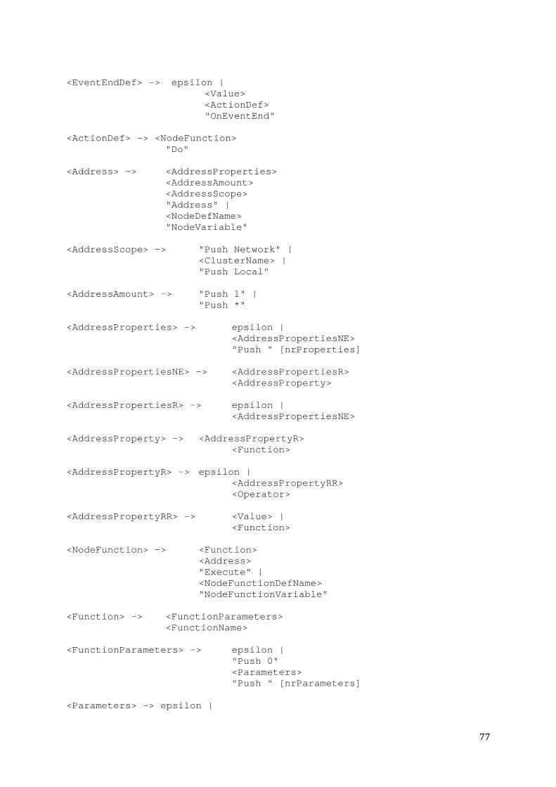
77  

<EventEndDef> -> epsilon | <Value> <ActionDef> "OnEventEnd" <ActionDef> -> <NodeFunction> "Do" <Address> -> <AddressProperties> <AddressAmount> <AddressScope> "Address" | <NodeDefName> "NodeVariable" <AddressScope> -> "Push Network" | <ClusterName> | "Push Local" <AddressAmount> -> "Push 1" | "Push *" <AddressProperties> -> epsilon |

<AddressPropertiesNE> "Push " [nrProperties]

<AddressPropertiesNE> -> <AddressPropertiesR>

<AddressProperty> <AddressPropertiesR> -> epsilon |

<AddressPropertiesNE> <AddressProperty> -> <AddressPropertyR> <Function> <AddressPropertyR> -> epsilon | <AddressPropertyRR> <Operator> <AddressPropertyRR> -> <Value> |

<Function> <NodeFunction> -> <Function> <Address> "Execute" | <NodeFunctionDefName> "NodeFunctionVariable" <Function> -> <FunctionParameters> <FunctionName> <FunctionParameters> -> epsilon | "Push 0"

<Parameters> "Push " [nrParameters] <Parameters> -> epsilon |

78  

<ParametersNE> <ParametersNE> -> <ParametersR> <Parameter> <ParametersR> -> epsilon |

<ParametersNE> <Parameter> -> <Value> <ParameterName> <Value> -> <NodeFunction> <ValueOp> | <Constant> <ValueOp> | <Variable> <ValueOp> <ValueOp> -> epsilon | <Value> <Operator> "Execute" <Variable> -> <VariableName> "Variable" <Operator> -> "Push 2" "Push " \"[Operator]\" <ServiceName> -> "Push " <Name> <ClusterName> -> "Push " <Name> <NodeDefName> -> "Push " <Name> <NodeFunctionDefName> -> "Push #"<Name> <ParameterName> -> "Push " <Name> <Constant> -> "Push " <Int> |

"Push " <Real> | "Push " String | <Address>

<VariableName> -> "Push $" <Name> <SubscriptionNameDef> -> "Subscription" <Name> <TopologyTypeNameDef> -> "Topology" <Name> ------------------------- <Name> -> String [Operator] -> "<" | "<=" | "=" | ">=" | ">" | "&&" | "||" |

"+" | "-" | "*" | "/"

79  

Appendix C: BYTECODE INSTRUCTIONS  This table provides an overview of the instructions of the bytecode described in Chapter 5.  Instruction  Meaning PUSH <Value> Pushes a value onto the general stack. SERVICE Starts the definition of a service. SUBSCRIPTION Starts the definition of a subscription. TOPOLOGY Starts the definition of a topology. FOR Indicates the address the command should be processed by. ADDRESS Indicates an address. DEFINENODE Sets an address as a node variable. DEFINENODEFUNC Sets a function executed on a node as a node function variable. ONEVENT Indicates an event condition. ONEVENTEND Indicates an event end condition. DO Indicates an action. VARIABLE Indicates a variable. NODEVARIABLE Indicates a node variable. NODEFUNCVARIABLE Indicates a node function variable. EXECUTE Indicates a function that should be executed. CONSTANT Indicates a constant. END Indicates the end of a command. Table 11: Overview of bytecode instructions