arX

iv:2

109.

1153

6v1

[ec

on.T

H]

23

Sep

2021

PERSUASION WITH AMBIGUOUS RECEIVER PREFERENCES

Eitan Sapiro-Gheiler

MIT

September 24, 2021

Abstract. I describe a Bayesian persuasion problem where Receiver has a private

type representing a cutoff for choosing Sender’s preferred action, and Sender has

maxmin preferences over all Receiver type distributions with a known mean. Sender’s

utility from any distribution of posterior means is a function of its concavification; this

result leads Sender to linearize the prior distribution by inducing a truncated uniform

distribution of posterior means. When the prior belief about the state of the world

is binary, Sender’s unique optimal distribution is an upper-truncated uniform with an

atom at 0. When the prior belief about the state of the world is continuous and uni-

modal, one optimal distribution for Sender is a double-truncated uniform with an atom

at the end of the lower truncation. In both cases, the shape and support of the optimal

distribution differ qualitatively from the corresponding solution when Sender holds a

prior belief over Receiver types.

JEL Classification: D81, D82, D83

Keywords: Bayesian persuasion, private information, maxmin utility

Email: eitans@mit.edu

I thank Drew Fudenberg, Sylvia Klosin, Stephen Morris, Victor Orestes, Frank Schillbach, Dmitry

Taubinsky, Rafael Veil, Jaume Vives, and especially Alexander Wolitzky for helpful discussions and

comments. This material is based upon work supported by the National Science Foundation Graduate

Research Fellowship under Grant No. 1745302.

1. Introduction

Consider a politician who is proposing a new welfare program. She must decide how to

disclose information about the expected cost of this proposal, but does not know how

much spending voters will support. All voters have the same ex-ante beliefs about the

program’s potential cost, but some will only approve if, after hearing the politician’s

message, they expect the cost to be low, while others are willing to support even a large

government outlay. Rather than imposing a prior distribution over people’s preferences,

the politician wishes to be robust to the worst-case distribution she may face. In this

setting, what disclosure rule maximizes the share of voters who, after hearing the politi-

cian’s message, approve of the welfare program? How does this optimal rule differ from

the case where the politician faces a known distribution of citizen preferences?

I address and generalize those questions through a model of Bayesian persuasion (Kamenica and Gentzkow,

2011), where a Sender commits to a message distribution in each state of the world and

a Receiver uses Bayesian updating to form a posterior belief about the state based on

the message structure. To represent different preferences among voters, I use private

Receiver types denoting the cutoff above which Receiver chooses Sender’s preferred ac-

tion. Sender knows the mean and range of Receiver types, and has maxmin preferences

(Gilboa and Schmeidler, 1989) over all Receiver type distributions satisfying those con-

straints. Regardless of the true state of the world, Sender maximizes the probability of

inducing the favorable action. This model captures situations where all Receiver types

process information in the same way, but may have different preferences over outcomes.

In addition to the political spending example described above, a model of this style also

applies to a variety of other situations, such as disclosing information about product

quality (if potential customers respond to product descriptions in the same way, but

may be more or less picky about quality) or screening job candidates (if all firms have

a common prior about candidate quality and see the same resume, but have different

thresholds for hiring).

In the standard Bayesian persuasion setting with a binary state of the world and a

log-concave prior distribution over Receiver cutoffs,1 Sender communicates either “good

news,” which makes Receiver more confident, but not certain, that the state is good; or

“worst news,” which makes Receiver certain that the state is bad. Doing so allows Sender

to generate credible good news as often as possible. However, when I replace that prior

with my chosen form of ambiguity preferences, I find that Sender may also communicate

1The case of a log-concave prior includes common specifications such as a normally-distributed prior

or a uniform prior over a (possibly degenerate) sub-interval of [0, 1].

1

“bad news,” which (analogously to good news) makes Receiver less confident that the

state is good, but not certain that it is bad.2 Intuitively, when facing ambiguity Sender

is less concerned about targeting a particular degree of good news (i.e., good news that

raises Receiver’s belief to a certain cutoff) and more interested in covering a broad range

of possible cutoffs. In fact, I show that all degrees of bad news, and all degrees of good

news below a known upper bound, are equally likely to arise.

In a richer setting where the state of the world is continuous and Sender’s prior belief

about it is unimodal, then this solution is no longer feasible, since it places strictly

positive probability on worst news while the prior does not. However, I can restore

feasbility and preserve optimality by adding a lower-truncation region, so that Sender

conveys an interval of intermediate beliefs with equal probability, but never induces

Receiver to believe that the state of the world is especially good or bad.3 This double

truncation again contrasts sharply with the case of a log-concave prior distribution over

Receiver types, where Kolotilin et al. (2017) show that Sender’s optimal strategy is to

fully reveal low states and pool high ones, leading to an atom and upper truncation

but no distortion of the prior distribution for low states of the world. As in the binary-

state case, the potential for an adversarial Receiver type distribution encourages Sender

to linearize the prior distribution and make different posterior beliefs about the mean

state of the world equally likely; however, the additional constraints imposed by the

continuous state space force Sender to generate a narrower interval of posterior means

in order to remain credible while doing so.

To derive my results, I solve the model by backwards induction, reframing Sender’s

maxmin preferences as a zero-sum game in which Sender chooses a distribution of pos-

terior means G for Receiver and then Nature chooses a Receiver type distribution T to

minimize Sender’s payoff. In this formulation, the known mean Receiver type r∗ makes

Nature’s problem analogous to Bayesian persuasion. Specifically, Nature behaves as if

facing a “prior distribution” of Receiver types with support {0, 1} and mean r∗, and

chooses a Bayes-plausible “posterior distribution” of Receiver types T to maximize the

opposite of Sender’s payoff. Thus the result of Kamenica and Gentzkow (2011) means

that for each G, Nature’s utility is given by the concavification ofG and Sender’s utility is

correspondingly given by the convexification of 1−G. This result suggests that a concave

2In a binary-state, binary-action model, for any prior distribution over Receiver types, there is a

binary-support posterior distribution that achieves Sender’s best payoff. Thus Sender may generate

good news and bad news, or good news and worst news, but never all three.3To preserve the appropriate average posterior mean belief, lower truncation changes the exact pos-

terior mean beliefs that arise; however, those beliefs still form a closed interval.

2

cdf of posterior means is best for Sender, and indeed in the binary-state case Sender’s

unique optimal posterior cdf is piecewise linear and concave. In the continuous-state

case, the need for the distribution of posterior means to be a mean-preserving contrac-

tion of the prior F prevents Sender from choosing that same solution, but I show that

adding a lower truncation region to that same piecewise linear shape restores feasibility

while preserving optimality. In both cases, distributions in the optimal class but with

different parameters can be used to approximate other candidate optimal distributions

near the mean Receiver type r∗; this result allows me to prove uniqueness of the opti-

mal distribution in the binary-state case, and provide some conditions on other possible

optimal distributions in the continuous-state case.

2. Related Literature

This work builds directly on the Bayesian persuasion problem originally described in

Kamenica and Gentzkow (2011), and adopts a similar approach to existing work in ro-

bust mechanism design. In addition, my model resembles a particular type of Colonel

Blotto game. I describe each of those areas in turn.

In the baseline Bayesian persuasion model of Kamenica and Gentzkow (2011), Receiver

has no private information. Subsequent literature in this area is surveyed in detail

by Kamenica (2019) and Bergemann and Morris (2019); in this section I focus on the

two works most directly related to the model I propose, Kolotilin et al. (2017) and

Hu and Weng (2020).4 The former has an interval state space, Receiver types that enter

payoffs linearly, and a binary action, as in my model; however, it endows Sender with

a prior distribution over Receiver types. If that prior distribution is log-concave, then

the optimal distribution for Sender can be generated by upper censorship; the resulting

distribution of posterior means is essentially a truncated version of the prior where states

in some interval [α, 1] are replaced with an atom at β ∈ (α, 1). In the continuous-state

case of my model, Sender seeks to linearize the posterior distribution to avoid facing

a tailored Receiver type distribution in response, and must use a double truncation to

make sure this strategy respects Bayes-plausibility.

The model of Hu and Weng (2020) is most similar to the one considered here: it is

a binary-action model where Sender has maxmin preferences over Receiver types and

4Other works use maxmin preferences in Bayesian persuasion settings, but are much more dis-

tinct. In Kosterina (2020), possible Receiver type distributions are distortions of a “reference dis-

tribution;” in Dworczak and Pavan (2020), there is full ambiguity about Receiver’s posterior belief; and

in Laclau and Renou (2017) and Beauchene et al. (2019), Receiver has maxmin preferences.

3

maximizes the probability of inducing the favorable action. However, Receiver types

represent an ambiguous posterior about a binary state of the world rather than a payoff-

relevant characteristic which does not directly interact with beliefs about the state.

This model captures substantively different applications—e.g., voters with common ide-

ology who privately read outside news sources before listening to a politician’s speech,

rather than the equally-informed voters with different ideological positions in my model.

Working with belief-independent Receiver types also means that I am able to charac-

terize Receiver’s posterior distribution and thus provide a sharp testable prediction—all

posteriors in a known interior interval are equally likely. Methodologically, because my

formulation features a simpler interaction between Receiver’s type and Sender’s signal,

I am able to extend my approach and characterization of Sender’s optimal policy to a

continuous-state case.

This work also relates to a literature in robust mechanism design, and in particular

works in which maxmin preferences are paired with moment conditions.5 For example,

Wolitzky (2016) considers a bilateral trade model where each agent has a valuation in

[0, 1] and knows only the mean of the other agent’s type distribution. In that model,

agents’ worst-case beliefs have binary support. Here, the worst-case Receiver type dis-

tribution is binary-support as well, but Sender’s desire to induce indifference between

many such distributions means the optimal posterior distribution has interval support.

Two other works consider distinct variations of the moment-restricted mechanism de-

sign problem. In Carrasco et al. (2019), a principal with maxmin preferences offers a

surplus-maximizing contract to a privately informed agent. Similar to my model, the

agent’s type distribution has known mean and support [0, 1]. As in Hu and Weng (2020)

and my work, the optimal mechanism for the principal induces a payoff that is piecewise

linear in the agent’s type. The other work, Carrasco et al. (2018), considers a setting

where a seller with maxmin preferences faces an unknown distribution of buyer valua-

tions in R+. The seller knows the first N − 1 moments of the buyer type distribution

and an upper bound on the Nth moment. Similar to the convexification argument I use,

transfers for the optimal mechanism are given by the non-negative monotonic hull of a

degree-N polynomial.

5Maxmin preferences more broadly have been used to model robustness in settings such as monopoly

pricing (Bergemann and Schlag, 2011), auctions (Bose et al., 2006), and screening contracts (Auster,

2018). Other work has focused on general results such as payoff equivalence (Bodoh-Creed, 2012) or

implementability (de Castro et al. 2017 and Ollar and Penta 2017).

4

Another antecedent of my model is the Colonel Blotto game, first proposed by Borel

(1921), where opposing players A and B simultaneously choose how to allocate their

troops across finitely many battlefields. Bell and Cover (1980) introduces a “continuous”

version called the General Lotto game, where A and B choose distributions FA and

FB of troops over a unit interval of battlefields. Mean constraints E[FA] = a and

E[FB] = b represent the amount of troops each player commands. In both versions,

each player maximizes the probability that, at a uniformly drawn battlefield, they have

allocated more troops than their opponent; in my setting Sender does not care about a

uniformly drawn Receiver type but rather a draw from the worst-case distribution for

each disclosure policy. Despite this difference in objective functions, the solution to the

asymmetric General Lotto game with a ≥ b > 0, due to Sahuguet and Persico (2006), is

almost identical to the binary-state case of my model. In the General Lotto game, player

A uniquely selects FA = U [0, 2a] while player B uniquely selects a uniform distribution

over (0, 2a] with an atom at 0 to meet their stricter mean constraint. In the binary-state

version of my model, if the prior belief that the state is high, π, exceeds the mean Reciever

type, r∗, then Sender uniquely chooses the posterior distribution U [0, 2π], analogously to

player A. If instead π < r∗, then Sender uniquely chooses an upper-truncated uniform

distribution with an atom at 0, similar to player B, but.its upper bound need not equal

2π. The intuition is that Sender makes Nature indifferent between any distribution

of Receiver types whose support is a subset of Sender’s chosen posterior distribution.

Higher Receiver types are no more unfavorable, but are more costly given the mean

constraint, so Nature does not generate them. Thus Sender endogenously faces the

same uniform draw as in the General Lotto game, but can choose the upper bound on

that draw to trade off their own mean constraint with Nature’s. However, in the General

Lotto game battlefields in [2a, 1] may still be drawn regardless of either player’s choice,

so the upper bound on the support is driven only by the less-constrained player.

3. Model

There is one Sender (she) and one Receiver (he).6 Sender knows the state of the world

ω ∈ [0, 1], and both players share a common prior belief F ∈ ∆([0, 1]) about the state

with E[F (ω)] = π ∈ (0, 1). Only Receiver knows his private type r ∈ [0, 1], but the

mean Receiver type r∗ ∈ (0, 1) is common knowledge. Sender holds maxmin preferences

6Alternatively, the presence of one Receiver with multiple unknown types may be interpreted as a

population of Receivers, each with a private type, with which Sender communicates publicly; this is the

interpretation I use for the political spending example.

5

over the set of potential Receiver type distributions T in the set

T =

{

cdf T over [0, 1]

∣

∣

∣

∣

∫

r dT (r) = r∗}

.

After Sender communicates, Receiver chooses a binary action a ∈ {0, 1}. Specifically,

Receiver chooses the high action if and only if his posterior expectation of the state,

q = E[ω | Sender’s behavior], strictly exceeds r:

uR(a, ω, r) = a (ω − r).

The explicit functional form used here is for ease of exposition only. Whenever Re-

ceiver’s utility is a linear function of the state, his action depends only on the mean

of his posterior belief about the state, and my results still hold (under an appropriate

renormalization of the interval of Receiver types). Substantively, the decision to break

ties against Sender is equivalent to assuming that there is some Receiver type who is

not persuaded even by knowing with certainty that ω = 1, and is discussed in greater

detail in Appendix A.

Sender’s goal is to maximize the probability of inducing the high action a = 1 indepen-

dent of the true state ω and true Receiver type r:

uS(a, ω, r) = a.

I restrict Sender to the standard Bayesian persuasion tool of committing ex-ante to a

(Blackwell) experiment, i.e., a state-dependent signal distribution, and in particular do

not allow her to elicit Receiver’s type in order to capture the public-communication

interpretation of this model. Since Receiver’s choice of action depends only on the mean

q of posterior belief distribution, I can, as in Kolotilin et al. (2017) and other similar

works, directly consider Sender choosing a distribution of posterior means G such that

G is a mean-preserving contraction of the prior distribution F . The set of feasible

distributions of posterior means is therefore

G =

{

cdf G over [0, 1]

∣

∣

∣

∣

∫

q dG(q) = π and

∫ x

0

G(q) dq ≤

∫ x

0

F (q) dq ∀ x ∈ [0, 1]

}

.

I follow the literature in referring to these two constraints jointly as Bayes-plausibility,

and reserve the expression “mean restriction” to refer to the condition on the set T of

Receiver type distributions.

Using this formulation and Receiver’s decision rule, I rewrite Sender’s utility as

uS(q, r) = 1(q > r),

6

so that Sender’s full optimization problem is

maxG∈G

{

minT∈T

∫ ∫

1(q > r) dG(q) dT (r)

}

. (1)

The main difference from standard Bayesian persuasion with private information is the

presence of an endogenously-determined Receiver type distribution F . This specification

leads me to characterize the solution by reframing Sender’s maxmin preferences as a zero-

sum game, in which Sender designs a posterior distribution and then Nature adversarially

designs a type distribution; that game can then be solved by backwards induction.7

When supp(F ) = {0, 1}, so that the state ω is binary, the second part of the Bayes-

plausibility constraint is redundant and any distribution G satisfying E[G] = π is in

G. This simplification permits a clearer characterization of the optimal distribution of

posterior means, which I present in Section 4. As in the case of Bayesian persuasion with

a prior belief about Receiver’s type, the binary-state solution generically places an atom

at q = 0. Thus when F lacks an atom at 0, as in the case of unimodal F that I study in

Section 5, that solution will not be Bayes-plausible. However, I will show that a simple

lower truncation of the binary-state solution—setting the cdf to 0 in a neighborhood of

q = 0, then adjusting the rest of the distribution to leave its mean unchanged—is often

sufficient to restore Bayes-plausibility while preserving optimality.

4. The Binary-State Case

In this section, I fully characterize Sender’s optimal distribution of posterior means when

the prior distribution F has binary support, so that a distribution of posterior means

is the same as a posterior distribution (I use the latter expression for simplicity) and

the only restriction imposed on Sender is that E[G] = π for any posterior distribution

G. I focus on the case where supp(F ) = {0, 1}, but under appropriate assumptions, all

results extend to the case where supp(F ) = {α, β} for 0 ≤ α < β ≤ 1; I discuss that

generalization in Appendix A.

I approach the problem in three steps. First, I show, by analogy to a Bayesian persua-

sion problem over Receiver types, that Sender’s utility from a posterior distribution G is

given by the convexification of 1− G. This step allows me to immediately characterize

7The maxmin specification means that Sender moves first, but when F has binary support, the

maxmin and minmax formulations are essentially identical since Sender and Nature’s constraints are of

the same type. In Appendix C, I discuss the relationship between the maxmin and minmax solutions

and provide conditions for a saddle-point solution where Sender’s maxmin-optimal posterior distribution

is also minmax-optimal.

7

Sender’s multiple optimal posterior distributions when π > 1/2; I do so in Proposition 1.

Next, I describe upper-truncated uniform distributions, whose cdfs are piecewise linear

and concave—and use the convexification result to solve explicitly for Sender’s unique

optimal upper-truncated uniform distribution as a function of the mean Receiver type.

Finally, when π ≤ 1/2 I use these distributions to approximate any candidate opti-

mal distribution, and in doing so show that Sender’s optimal upper-truncated uniform

distribution is in fact uniquely optimal overall.

4.1. Characterizing the Distribution of Receiver Types. To characterize Sender’s

utility as a function of the mean Receiver type r∗ without using a specific Receiver type

distribution, Lemma 1 draws an analogy between the objective function of Equation (1)

and Bayesian persuasion over Receiver types.

Lemma 1. For a given posterior distribution G, let G : [0, 1] → [0, 1] be the concav-

ification of G, i.e., the infimum over the set of concave functions H : [0, 1] → [0, 1]

satisfying

H(q) ≥ G(q) ∀q ∈ [0, 1].

Then the following equality holds:

minT∈T

∫ ∫

1(q > r) dG(q) dT (r) = 1− H(r∗).

The result can equivalently be expressed through the convexification of 1 − G, i.e., the

supremum among convex functions that lower-bound 1 − G; this framing is used in

Hu and Weng (2020), which proves a similar result for a finite state space. Both their

proof and mine invoke the result of Kamenica and Gentzkow (2011) to characterize the

solution of the Bayesian persuasion problem without private information.

Proof. Manipulating the bounds of integration to rewrite Sender’s objective function

from Equation (1) gives∫

[0,1]

(∫

[0,1]

1(q > r) dG(q)

)

dT (r) =

∫

[0,1]

(∫

[r,1]

1 dG(q)

)

dT (r)

=

∫

[0,1]

(1−G(r)) dT (r).

Then the minimzation portion of the problem can be written as

maxT∈∆([0,1])

∫

G(r) dT (r) s.t.

∫

r dT (r) = r∗,

8

where I have dropped the constant, rewritten the min as a max, and explicitly included

the mean restriction to highlight the similarity to a Bayesian persuasion problem. In

this case, the Receiver type r fills the role of “posterior belief,” Nature’s utility from a

realized Receiver type is G(r), and the “prior” is the distribution with support {0, 1}

and mean r∗. This final point follows from the observation in Section 3 that when the

prior distribution has binary support, the Bayes-plausibility constraint is the same as

a mean restriction. Thus by Corollary 2 of Kamenica and Gentzkow (2011), Nature’s

utility is given by G. the concavification of G over the interval [0, 1], evaluated at the

prior mean r∗. Flipping the sign again, Sender’s utility is 1− G(r∗), or equivalently the

convexification of 1−G over the interval [0, 1] evaluated at r∗. �

This lemma does not require that F have binary support, and will apply unchanged in

Section 5. However, in this case it is immediately useful in solving for Sender’s optimal

posterior distribution when π > 1/2:

Proposition 1. Let π > 1/2. Then any feasible posterior distribution G ∈ G is optimal

for Sender if and only if it satisfies

G(q) ≤ q ∀ q ∈ [0, 1],

and more than one distribution satisfying this condition exists.

The details of the proof are in Appendix B, but the idea is straightforward. Letting

U denote the uniform distribution U [0, 1], Sender’s utility is always upper-bounded by

1 − U , which is both the convexification of 1 − U and the largest convex function on

[0, 1] passing through the point (1, 0). When π < 1/2, U is not Bayes-plausible, and

Sender must induce relatively more low posteriors than she would under U . However,

when π > 1/2, Sender can achieve the upper bound with any posterior distribution that

first-order stochastically dominates U . One distribution satisfying that condition is

G(q) =

0 q ∈ [0, 2π − 1),

(q + 1− 2π)/(2− 2π) q ∈ (2π − 1, 1].

G is a lower-truncated uniform distribution with no mass on posteriors q ∈ [0, 2π − 1)

and equal mass on all posteriors q ∈ [2π − 1, 1]. In Proposition 2, I show that when

π ≤ 1/2, Sender’s optimal posterior distribution is unique, but in this case there are

many other Bayes-plausible distributions whose concavifications equal U . For example,

setting π = n/(n + 1) and solving for n gives a cdf G(q) = qn that is Bayes-plausible

and satisfies G(q) ≤ q. Thus Sender’s optimal posterior distribution when π > 1/2 is

9

not unique. However, her maxmin utility as a function of the mean Receiver type r∗ is

uniquely given by U(r∗) = 1− r∗ regardless of which posterior distribution is chosen.

4.2. Upper-Truncated Uniform Distributions. When π ≤ 1/2, a distribution G

for which G = U would violate Bayes-plausibility. It is intuitive for Sender to respond

to this limitation by choosing a posterior distribution G with a concave cdf, since by

Lemma 1 any non-convexities in 1 − G tighten Bayes-plausibility without raising her

utility. Motivated by that idea, in this section I introduce and describe upper-truncated

posterior distributions (henceforth UTUs), a class of posterior distributions which are

piecewise linear with concave cdf. A UTU places mass x ≥ 0 on posterior q = 0, equal

mass on all posteriors q ∈ (0, rh] for some rh ≤ 1, and no mass on posteriors q ∈ (rh, 1].

The cdf of a UTU is therefore composed of an upward-sloping line from (0, x) to (rh, 1)

and a horizontal line from (rh, 1) to (1, 1), and is thus concave. Given this structure, I

can use Bayes-plausibility to solve for the unique value of rh corresponding to a given

x, so that a UTU is fully characterized by x. Thus I denote a UTU by Gx, and write

rh(x) for the upper bound on its support.

To solve for rh(x), I use Bayes-plausibility to write

π =

∫

q dGx(q) =

∫

1−Gx(q) dq =(1− x) rh(x)

2

⇔ rh(x) =2π

1− x,

where I integrate by parts to obtain the second integral, then use the shape of G to write

the area under 1−G(q) as a triangle with base rh(x) and height 1−x. Since I have already

characterized Sender’s optimal posterior distribution when π > 1/2 in Proposition 1, I

assume π ≤ 1/2; then this expression implies an upper bound of 1− 2π ≥ 0 on x, since

otherwise rh(x) would exceed 1, but allows x to take any value in [0, 1− 2π]. The UTU

G1−2π for which x meets the upper bound places equal mass on all posteriors q ∈ (0, 1];

it will play a key role in characterizing Sender’s optimal posterior distribution.

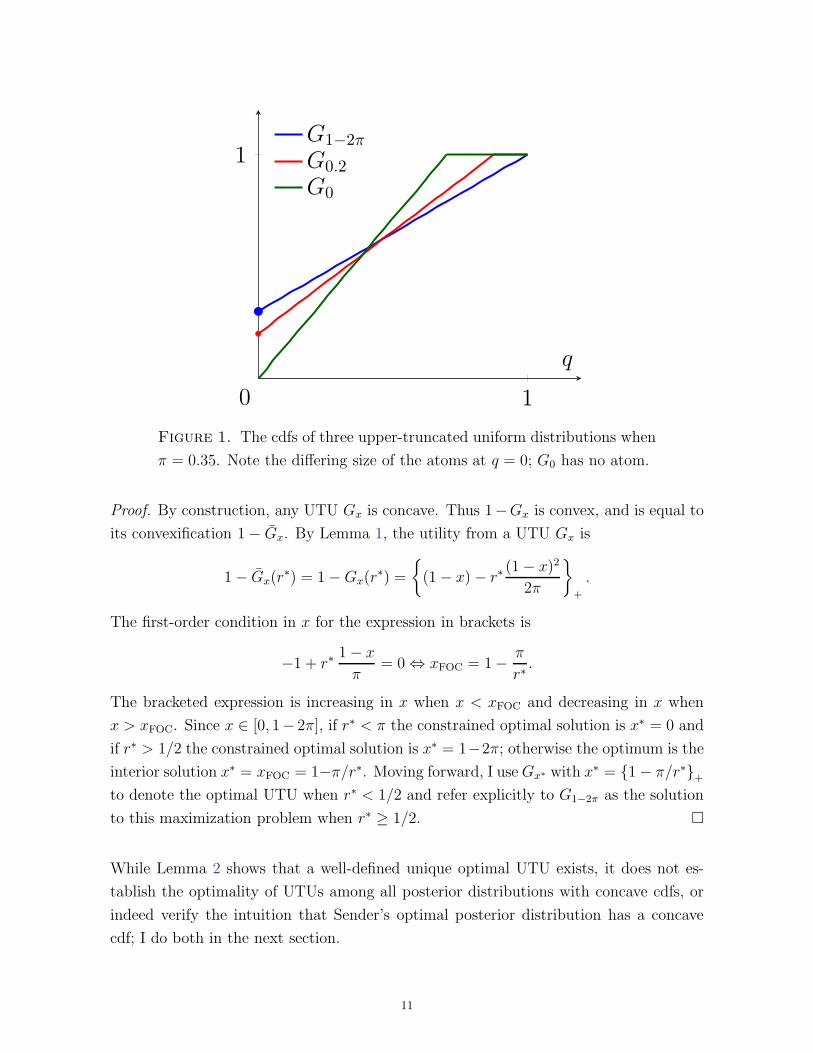
Figure 1 shows an example of three UTUs, including G1−2π. The figure suggests that no

UTU lies below another for all q ∈ [0, 1], and therefore that Sender’s optimal UTU may

vary with the model parameters. Lemma 2 formalizes this intuition by characterizing

Sender’s optimal UTU as a function of the mean Receiver type r∗:

Lemma 2. Let π ≤ 1/2. Then if r∗ ≥ 1/2, Sender’s unique optimal UTU is G1−2π, and

if r < 1/2, Sender’s unique optimal UTU is Gx∗ where x∗ = {1− π/r∗}+.

10

1

1

0

q

G1−2π

G0.2

G0

Figure 1. The cdfs of three upper-truncated uniform distributions when

π = 0.35. Note the differing size of the atoms at q = 0; G0 has no atom.

Proof. By construction, any UTU Gx is concave. Thus 1−Gx is convex, and is equal to

its convexification 1− Gx. By Lemma 1, the utility from a UTU Gx is

1− Gx(r∗) = 1−Gx(r

∗) =

{

(1− x)− r∗(1− x)2

2π

}

+

.

The first-order condition in x for the expression in brackets is

−1 + r∗1− x

π= 0 ⇔ xFOC = 1−

π

r∗.

The bracketed expression is increasing in x when x < xFOC and decreasing in x when

x > xFOC. Since x ∈ [0, 1− 2π], if r∗ < π the constrained optimal solution is x∗ = 0 and

if r∗ > 1/2 the constrained optimal solution is x∗ = 1−2π; otherwise the optimum is the

interior solution x∗ = xFOC = 1−π/r∗. Moving forward, I useGx∗ with x∗ = {1− π/r∗}+to denote the optimal UTU when r∗ < 1/2 and refer explicitly to G1−2π as the solution

to this maximization problem when r∗ ≥ 1/2. �

While Lemma 2 shows that a well-defined unique optimal UTU exists, it does not es-

tablish the optimality of UTUs among all posterior distributions with concave cdfs, or

indeed verify the intuition that Sender’s optimal posterior distribution has a concave

cdf; I do both in the next section.

11

4.3. Optimality of Upper-Truncated Uniform Distributions. The main result of

this section is that when π ≤ 1/2, Sender’s optimal posterior distribution is the optimal

UTU from Lemma 2.

Proposition 2. Let π ≤ 1/2. Then if r∗ ≥ 1/2, Sender’s unique solution G∗ to the

persuasion problem of Equation (1) is

G∗(q) = G1−2π(q) =

1− 2π q = 0,

1− 2π + 2πq q ∈ (0, 1].

If r∗ < 1/2, it is

G∗(q) = Gx∗(q) =

x∗ q = 0,

x∗ + q (1− x∗)2/(2π) q ∈ (0, 2π/(1− x∗)],

1 q ∈ (2π/(1− x∗), 1],

where x∗ = {1− π/r∗}+.

The full proof is in Appendix B; I provide an intuition here. Consider a posterior

distribution H that weakly improves on Sender’s utility from G∗; by Lemma 1, it must

be that 1 − H(r∗) ≥ 1 − G∗(r∗). Because 1 − H is convex, it can be lower-bounded by

the line L tangent to it at r∗, and more specifically by L+ since 1− H is weakly positive.

Let H ′ be a posterior distribution such that 1−H ′ = L+; the key step of the proof is to

show that H ′ violates Bayes-plausibility because its mean is too large. Then, because∫

q dH(q) =

∫

1−H(q) d(q)

≥

∫

1− H(q) dq ≥

∫

L+(q) dq =

∫

1−H ′(q) dq =

∫

q dH ′(q),

it must be thatH also violates Bayes-plausibility and is thus an invalid choice for Sender.

To show the violation of Bayes-plausibility, I exploit properties of the convexification

1− H and of UTUs. Because G∗ is optimal among UTUs, it is the case that

1− H(r∗) ≥ 1− G∗(r∗) ≥ 1− G1−2π(r∗) = 1−G1−2π(r

∗).

Therefore, the convexity of 1 − H ensures that 1 − H must lie above 1 − G1−2π on the

interval [0, r∗). To obey Bayes-plausibility, 1 − H must eventually lie below 1 −G1−2π,

so the slope of H at r∗ (and therefore of its tangent line L) must be less than that

of 1 − G1−2π. The lesser slope of L+ compared to 1 − G1−2π ensures that L+(0) >

1−G1−2π(0). Thus there exists an UTU, GxH, satisfying L+(0) = 1−GxH

(0). But since

12

1

1

0

uS

r∗

q

1−G∗

L+

1−GxH

Figure 2. Sender’s utility from the proposed optimal posterior distribu-

tion G∗ compared to the tangent line L+ and the distribution GxH.

L+(r∗) = 1− H(r∗) and 1− H(r∗) represents an improvement on Sender’s utility from

the best UTU, it must be that L+(r∗) > 1−GxH

(r∗), and thus the slope of L+ is greater

than that of 1−GxH.8 This relationship between 1−Gx∗ , L+, and 1−GxH

is shown in

Figure 2. Since UTUs satisfy Bayes-plausibility by construction, the area under L+ is

too large, producing the desired violation of Bayes-plausibility.

Proposition 2 shows that supp(G∗) is a closed interval with lower endpoint at 0 that con-

tains π in its interior, resulting in the “good news, bad news, worst news” interpretation

described in the introduction. When r∗ > π, so that Sender’s Bayes-plausibilty con-

straint is stronger than Nature’s mean restriction, the distribution has an atom at 0 and

worst news is realized with strictly positive probability. Regardless of whether that oc-

curs, the distribution G∗ is uniform over supp(G∗) \ 0: all degrees of good and bad news

are equally likely. This result also verifies the intuition that, when Bayes-plausibility

forces Sender to generate more low posteriors than under a uniform distribution, she

chooses a concave posterior distribution to avoid “wasting” posterior mass. Linearity of

the optimal posterior distribution is in turn a consequence of the specific form of Sender

and Receiver’s utility functions. Because Sender cares equally about all Receiver types,

8There is a slight subtlety here, since when r∗ < 1/2, it may be that GxH= G∗ and (if H matches

Sender’s utility from G∗) that L+(r∗) = 1−GxH

(r∗). However, 1−H must lie above 1−G∗ somewhere

in [0, 1] in order for H to be distinct, and I can show the violation of Bayes-plausibility using this fact.

13

and the share of Receiver types persuaded to choose action a = 1 increases linearly in

the posterior, Sender’s gain from a higher posterior belief is constant. Also as a result

of this linearity, Nature is indifferent between any choice of Receiver types in supp(G∗).

This result will play a key role in the minmax problem of Appendix C; similar indiffer-

ence results for either Nature or the designer appear commonly in maxmin mechanism

design, e.g., in Bose et al. (2006), Carrasco et al. (2019), and Brooks and Du (2021).

4.4. Comparative Statics of Sender’s Utility. Having characterized Sender’s opti-

mal posterior distribution, her utility follows from applying Lemma 1:

Corollary 1. If π ≤ 1/2, then Sender’s maxmin utility is given by

uS(π, r∗) =

1− r∗/(2π) r∗ ∈ (0, π),

π/(2r∗) r∗ ∈ [π, 1/2),

2π − 2πr∗ r∗ ∈ [1/2, 1).

If π > 1/2, then it is given by

uS(π, r∗) = 1− r∗.

A dramatic feature of this result is that, no matter how weak the Bayes-plausibility

constraint, Sender does no better than if Receiver acted on a uniformly drawn belief with

no further information. Regardless of the parameters, replacing the maxmin criterion

with any prior belief that does not first-order stochastically dominate U [0, 1] would result

in strictly higher utility for Sender; no prior belief would result in strictly lower utility.9

Comparative statics in the prior π and mean Receiver type r∗ follow naturally from

the closed-form expression in Corollary 1. Sender’s utility is continuous and strictly

decreasing in r∗ for fixed π, and continuous and weakly increasing in π for fixed r∗.10

Both comparative statics match the economic intuitions of the problem: if Receiver

has a higher prior belief that Sender’s welfare program will be under-budget, or Sender

knows average Receiver is more fiscally liberal, then Sender expects to convince more

Receivers to purchase her product. In fact, a low prior and low mean Receiver type

are “substitutes,” in that a high prior can compensate Sender for the harms of a high

9This result is a straightforward application of the usual concavification argument. In the proof of

Proposition 1, the uniform distribution generates the largest possible convexification; here it generates

the smallest possible concavification.10Specifically, her utility for fixed r∗ is strictly increasing when π ∈ (0, 1/2] and weakly increasing

when π ∈ (1/2, 1).

14

mean Receiver type, and a low mean Receiver type can compensate Sender for the

harms of a high prior. Given any two mean Receiver types r∗1 ≤ r∗2, it is clear from the

functional form of uS that there are two priors π1 ≤ π2 such that uS(π1, r∗1) = uS(π2, r

∗2).

Similarly, given priors I can choose mean Receiver types to get the same result.11 This

substitutability suggests that, in practice, it may be challenging to distinguish the effect

of a changing state of the world from that of changing Receiver attitudes.

5. The Continuous-State Case

In this section, I extend the insights of the binary-state model to the case where F

is a continuously differentiable and unimodal distribution over [0, 1] with F (0) = 0.

Specifically, I assume that, for some mode m ∈ (0, 1), the derivative f of F is strictly

increasing on [0, m) and strictly decreasing on (m, 1]. I also require that F does not

first-order stochastically dominate U [0, 1]. Otherwise, a direct analogue of Proposition

1 shows that, since the concavification of F is the cdf of U [0, 1], Sender cannot improve

on her utility from full disclosure.

The main difference between this setting and the binary-state case of Section 4 is that

Bayes-plausibility now constrains not only the expectation of any feasible distribution

of posterior means G, but also the integral of the cdf of G:∫ x

0

G(q) dq ≤

∫ x

0

F (q) dq ∀ x ∈ [0, 1].

I refer to this additional restriction as the “integral constraint” on G. Because of this

constraint, UTUs are no longer Bayes-plausible, since they have an atom at 0 while F

does not. To ensure that the UTU G0, which has no atom at q = 0, is not Bayes-

plausible, I assume that f(0) < 1/(2π) whenever the latter quantity is strictly positive.

One natural way to adapt UTUs is to use double-truncated uniform distributions, or

DTUs, whose cdfs are of the form

G(q) =

0 q ∈ [0, ℓ),

βq + y q ∈ [ℓ, (1− y)/β),

1 q ∈ [(1− y)/β, 1],

so that the distribution places no mass in the intervals [0, ℓ) (the lower truncation) and

[(1− y)/β, 1] (the upper truncation); Figure 3 shows an example of several DTUs.

11It is not true that given π1 and r∗1 ≤ r∗2 , I can find π2 such that uS(π1, r∗

1) = uS(π2, r∗

2). To see

why, note that uS(π2, r∗

2) ≤ 1 − r∗2 for any π2. Then there is π1 large enough that uS(π1, r∗

2) > 1− r∗2 ,

so that no π2 will compensate Sender for the difference in utility.

15

1

1

0

q

G1/40

G1/100

G1/41/5

Figure 3. The cdfs of three double-truncated uniform distributions when

π = 1/3. The blue and green DTUs G1/40 and G

1/100 have the same y-

intercept but different lower truncations; the blue and red DTUs G1/40 and

G1/41/5 have different y-intercepts but the same lower truncation.

A DTU clearly obeys the integral constraint for x ∈ [0, ℓ), but may violate it if the

atom at ℓ and the slope thereafter are too large; determining when this violation occurs

will be at the core of my characterization of optimal posterior distributions. Since the

additional parameter ℓ allows for a continuum of DTUs at each fixed intercept y (with

the slope β given as a function of y and ℓ), I first characterize the y-optimal DTU—the

utility-maximizing DTU among all Bayes-plausible DTUs with intercept y. When r∗ is

sufficiently small or sufficiently large, the y-optimal DTU has minimal slope among all

Bayes-plausible DTUs with intercept y. This result allows me to prove Proposition 3,

which establishes optimality of DTUs:

Proposition 3. Let r∗ ∈ (0, q1(ℓ∗0, 0)] ∪ [π, 1). Then no distribution of posterior means

gives Sender strictly higher utility than all double-truncated uniform distributions.

The value q1(ℓ∗0, 0) is a function of the lower-truncation length of the 0-optimal DTU, and

is defined in Corollary 2. As with Proposition 2 in the binary-state case, the core of the

result is a local approximation of any candidate optimal distribution by a piecewise linear

one. However, the presence of the lower truncation means I can no longer use a Bayes-

plausible DTU as a global bound on that approximating distribution. In the absence

16

of this bound, and since Sender’s utility depends only on the value of the concavified

posterior mean distribution at r∗, she is free to construct a non-DTU optimal distribution

by varying the mass placed in and around the lower truncation interval. In Section 5.3,

I show an example of one such distribution, and highlight its connection to the challenge

of characterizing optimal posterior mean distributions for intermediate values of r∗.

Towards proving Proposition 3, I characterize y-optimal DTUs in the following section.

I then prove the proposition, after which I return to the question of how the need for a

lower truncation region allows Sender greater flexibility than in the binary-state case.

5.1. Double-Truncated Uniform Distributions. As with the upper truncation and

atom size of the UTUs in Section 4.2, the requirement that any Bayes-plausible DTU

have mean π allows me to define β as a function of ℓ and y; I thus denote a generic DTU

by Gℓy.

12 When y ∈ [0, 1− 2π], any ℓ ∈ [0, π] generates a valid DTU, with the DTU Gy0

being the same as the UTU with atom y at posterior mean q = 0. When y ∈ (1− 2π, 1)

there is a value ℓminy > 0 which generates a DTU passing through the point (1, 1); this

value lower-bounds the valid choices of ℓ.

For any given mean Receiver type r∗ and intercept y, standard continuity arguments

applied to the cdf of Gℓy and its integral show that there exists some DTU G∗

y which

maximizes Sender’s utility among all DTUs with intercept y; this result is Lemma 7

in Appendix D. I call any such DTU y-optimal, to distinguish from a potential overall-

optimal DTU which maximizes Sender’s utility among all DTUs. Unlike the binary-state

case, it is not possible to solve analytically for G∗y without specifying a functional form

for F . However, appropriate sufficient conditions can ensure that G∗y is both unique and

slope-minimizing among Bayes-plausible DTUs with intercept y:

Lemma 3. Fix y ∈ [0, 1) and r∗ ∈ (0, 1). There is a unique and well-defined DTU Gsmy

that has minimal slope among all Bayes-plausible DTUs with intercept y. If y = 0 or

r∗ ∈ [π, 1), then the y-optimal DTU G∗y equals Gsm

y

The full proof is in Appendix D; I sketch it here. In the first case, setting y = 0 ensures

that the concavification of Gsm0 does not have a kink at q = ℓ; then, regardless of the

value of r∗, slope-minimization subject to Bayes-plausibility is best for Sender. In the

second case, setting r∗ ≥ π ensures that r∗ exceeds any valid choice of ℓ; then the kinked

concavification does not affect Sender’s utility.

12The explicit relationship, as well as other technical properties of DTUs, are presented alongside

relevant proofs in Appendix D.

17

This result allows me to simplify the integral constraint by identifying if and where it

binds. Let Qℓy be the set of interior points q ∈ (0, 1) where the line given by the uniform

portion of the DTU Gℓy intersects the prior F :

Qℓy = {q ∈ (0, 1) | β(ℓ, y) q+ y = F (q)} .

Under the sufficient condition on r∗ above, I can show that either the integral constraint

binds only at the minimum value of q in Qℓy, or it does not bind anywhere in (0, 1).

Lemma 4. Let Gsmy be the DTU with the minimal slope among all Bayes-plausibile

DTUs with intercept y, and let ℓsmy be its lower truncation. If y ∈ [0, 1 − 2π], then

q1(ℓ, y) = minQℓy is well-defined and ℓsmy satisfies

∫ q1(ℓsmy ,y)

0

F (q) dq =

∫ q1(ℓsmy ,y)

0

Gsmy (q) dq

and∫ x

0

F (q) dq >

∫ x

0

Gsmy (q) dq ∀x ∈ (0, q1(ℓ

smy , y)) ∪ (q1(ℓ

smy , y), 1).

If instead y ∈ (1 − 2π, 1), then either the condition above is satisfied, or ℓsmy equals the

minimum lower truncation length ℓmin

y .

The proof, which is in Appendix D, relies crucially assumptions about the shape of

the prior F . In particular, since F is strictly convex on [0, m) and strictly concave

on (m, 1], extending the linear portion of a DTU produces a line that intersects F at

most twice on (0, 1]. If that line lies weakly above F , then the corresponding DTU is

Bayes-plausible—in the interval [0, ℓ) the DTU lies below F , and in the interval [ℓ, 1]

the difference between the integral of F and that of the DTU decreases monotonically

and reaches 0 at q = 1. If instead the line intersects F twice, then the DTU may

increase too quickly in the interval (ℓ, 1] to be Bayes-plausible. Examining the geometric

relationship between F and such a DTU, Gℓy, shows that the difference between their

integrals is minimized at q1(ℓ, y). Thus a two-intersection DTU is Bayes-plausible if

and only if its integral is weakly less than that of F at q1(ℓ, y). When the relationship

holds with equality, the DTU is slope-minimizing among Bayes-plausible DTUs. When

y ∈ [0, 1− 2π], the smallest value of ℓ produces a UTU, which is not Bayes-plausible, so

there is always a DTU satisfying the given property. When instead y ∈ (1 − 2π, 1), it

may be that the minimal value of ℓ produces a DTU that lies weakly above F on [ℓ, 1]

and is therefore Bayes-plausible.

18

Lemma 4 can also be used as a key step in deriving the continuity of ℓ∗y in y, and thus in

providing sufficient conditions for the existence of an overall-optimal DTU (e.g., Lemma

8 in Appendix D). As an immediate corollary, it also allows a characterization of the

overall-optimal DTU when r∗ is small:

Corollary 2. Let ℓ∗0 be the length of the lower truncation for the 0-optimal double-

truncated uniform distribution G∗0, and let q1(ℓ

∗0, 0) be the smallest q ∈ (0, 1) that satisfies

β(ℓ∗0, 0) q = F (q).13 If r∗ ≤ q1(ℓ∗0, 0), then G∗

0 is uniquely optimal among all double-

truncated uniform distributions.

Proof. The proof is by contradiction, and resembles the proof of Proposition 2 in the

binary-state case. Fix r∗ and assume some other DTU G does weakly better than G∗0

for Sender. It must therefore have a smaller slope than G∗0: the intercept of G is larger

than that of G∗0, and G must intersect the horizontal line y = 1 at a larger value of q

than G∗0 or the concavification of G would be everywhere above that of G∗

0. Because of

its larger slope, G∗0 upper-bounds G after r∗ (where G lies weakly below G∗

0) and thus∫ 1

r∗G(q) dq <

∫ 1

r∗G∗

0(q) dq

⇒

∫ 1

q1(ℓ∗0 ,0)

G(q) dq <

∫ 1

q1(ℓ∗0,0)

G∗0(q) dq

⇒

∫ q1(ℓ∗0,0)

0

G(q) dq >

∫ q1(ℓ∗0,0)

0

G∗0(q) dq =

∫ q1(ℓ∗0,0)

0

F (q) dq.

The inequality in the first line is strict because F (q1(ℓ∗0)) < 1, so r∗ is not in the upper-

truncated region of G and there is some strict difference between G∗0 and G captured in

the integral. The first implication follows from the bound on r∗. The inequality in the

third line is because all DTUs have equal means, so

1− π =

∫ 1

0

G(q) dq =

∫ q1(ℓ∗0)

0

G(q) dq +

∫ 1

q1(ℓ∗0)

G(q) dq

=

∫ 1

0

G∗0(q) dq =

∫ q1(ℓ∗0)

0

G∗0(q) dq +

∫ 1

q1(ℓ∗0)

G∗0(q) dq.

The equality in the third line is by Lemma 4, since by Lemma 3 the DTU G∗0 has minimal

slope among Bayes-plausible DTUs with intercept 0. �

This result is similar to the optimal posterior distribution when π > r∗ in the binary-

state case (and indeed that optimal distribution is the DTU G00, which is only ruled out

13The existence of q1(ℓ∗

0, 0) is guaranteed by the proof of Lemma 4.

19

here by Bayes-plausibility). When r∗ is small relative to π, it is more costly for Nature

to generate high Receiver types than for Sender. Thus Sender focuses on the shape of

her optimal distribution near q = 0 at the cost of inducing fewer high posterior beliefs.

When the state is binary, this approach allows Sender to eliminate the atom at q = 0; in

this continuous-state case, Sender can reduce the size of the atom at q = ℓ. While in the

binary-state case the size of the atom increases with the value of r∗, the ability to vary

both ℓ and y in the continuous-state case means that such a result is more challenging

to establish, and may only hold after further restricting the prior distribution F .

5.2. Optimality of Double-Truncated Uniform Distributions. While a clearer

characterization of the optimal DTU outside the small-r∗ case is impeded by the greater

flexibility of the continuous-state problem, the simplified integral constraint in Lemma 4

can be directly combined with the bounding argument in Corollary 2 to prove Proposition

3. Recall that the proposition states that, for r∗ ∈ (0, q1(ℓ∗0)]∪ [π, 1)—i.e., small enough

for G∗0 to be the overall-optimal DTU or large enough to lie beyond the lower truncation

region—no distribution of posterior means gives Sender strictly higher utility than all

double-truncated uniform distributions. Before presenting the proof, I note that in some

cases q1(ℓ∗0) ≥ π, so that the restriction on r∗ is moot. A sharp characterization of when

this inequality is satisfied is not possible, as it depends greatly on the prior distribution

F , but it does arise in important cases like that of a truncated-normal F .

Proof. Let H be a candidate optimal distribution of posterior means. I approximate H ,

the concavification of H , by a tangent at r∗, which I call L(q); let L(0) = yL ∈ [0, 1) be

its intercept. Consider the yL-optimal DTU G∗yL. In order for H to do at least as well

for Sender as GyL, by Lemma 1 it must be that

1−H(r∗) ≥ 1− H(r∗) ≥ 1−G∗yL(r∗).

Thus L must have a weakly smaller slope than GyL, since otherwise L(r∗) > G∗yL(r∗)

and the above inequality is violated.

Recall that if yL ∈ [0, 1−2π], there are DTUs with any slope β ∈ ((1−yL)2/(2π), β(ℓ∗yL)],

and if yL ∈ (1 − 2π, 1), there are DTUs with any slope β ∈ [1− yL, β(ℓ∗yL)]. In the first

case, the slope of L cannot lie below that interval or it would have a weakly smaller

slope than the UTU with intercept yL; then the argument of Proposition 2 applies and

H is not Bayes-plausible. In the second case, L must have a slope that is weakly greater

than the lowest-slope DTU with intercept yL, or it would fail to pass through (1, 1), and

therefore so would H and H . Thus there is a DTU, GL, with the same slope as L.

20

Let r∗ ∈ (0, q1(ℓ∗0)]. By Corollary 2, if GL 6= G∗

0, then because GL(r∗) ≤ G∗

0(r∗), GL is

not Bayes-plausible. If instead r∗ ∈ [π, 1) and GL has a strictly smaller slope than GyL,

then by Lemma 3, GL is not Bayes-plausible.

In either case, given that GL violates Bayes-plausibility, H must violate it as well.

Because GL upper-bounds H beyond ℓ, it must be that∫ 1

q

H(t)dt ≤

∫ 1

q

H(t)dt ≤

∫ 1

q

GL(t)dt

for any q ∈ [ℓ, 1]. Since GL violates Bayes-plausibility, there is some qv ∈ [0, 1] where∫ qv

0

GL(t)dt >

∫ qv

0

F (t)dt,

and since the left-hand side equals 0 for any q ∈ [0, ℓ), it must be that qv ∈ [ℓ, 1]. Then

because H and GL have the same mean,∫ 1

0

H(t)dt =

∫ 1

0

GL(t)dt = 1− π

⇒

∫ qv

0

H(t)dt+

∫ 1

qv

H(t)dt =

∫ qv

0

H(t)dt+

∫ 1

qv

H(t)dt

⇒

∫ qv

0

H(t)dt ≥

∫ qv

0

GL(t)dt >

∫ qv

0

F (t)dt,

where the third line follows from the earlier upper bound on the integral of H . Therefore

H violates Bayes-plausibility and is not a valid distribution.

If GL has the same slope as GyL, then by construction H gives Sender the same utility

as GyL . Thus if there is a DTU that delivers Sender a strictly higher utility than GyL,

then clearly H is not optimal overall. If there is no such DTU, then GyL is optimal

among all DTUs and H also attains Sender’s maxmin utility. �

As in the binary-state case, Sender benefits from creating a large interval where poste-

rior means are uniformly distributed, since any binary-support Receiver type distribution

supported in this interval is equally bad. One way to generate a large interval that com-

plies with the integral constraint is by adding a lower truncation region to the UTUs of

Section 4. As in the binary-state case, the resulting DTU upper-bounds any alternative

distribution of posterior means in the interval [r∗, 1]. However, the lower truncation

region means that the concavification of a DTU lies above the DTU itself, unlike a UTU

which equals its concavification. Thus the DTU is no longer a global upper bound on

all candidate optimal distributions, and in fact Sender can even choose a distribution

21

whose concavification differs from that of a DTU around the lower-truncation region.

Such distributions are the focus of the following section.

5.3. Beyond Double-Truncated Uniform Distributions. Proposition 3 provides

only a mild condition on non-DTU optimal distributions: their slope at r∗ must equal

that of the overall-optimal DTU, if one exists. Using the tighter characterization of the

overall-optimal DTU in Corollary 2, I can strengthen the result in Proposition 3 for low

values of r∗ by giving a more explicit description of the concavification of H :

Corollary 3. Let r∗ ∈ (0, q1(ℓ∗0)]. Then, for any optimal distribution of posterior means

H, the concavification H of H is the same as the concavification G∗0 of the overall-optimal

double-truncated uniform distribution G∗0.

Proof. By the proof of Proposition 3, the slope of H at r∗ equals that of G∗0. In fact,

because G∗0 does not have a kink at ℓ∗0, it upper-bounds H on the whole interval [0, 1].

If H < G∗0 on any measurable subset of [r∗, 1] the proof of Corollary 2 shows that H

violates the Bayes-plausibility integral constraint at q1(ℓ∗0, 0).

If ℓ∗0 ≤ r∗, it is therefore true that H = G∗0 = G∗

0 on [r∗, 1]. Furthermore, G∗0 upper-

bounds H on [0, r∗] and G∗0(0) = H(0) = 0. Because G∗

0 is linear on [0, r∗] (i.e., it has

no kink at ℓ∗0) there is no smaller concave function that takes the same values at q = 0

and q = r∗; thus H = G∗0 on [0, r∗] as well.

If instead ℓ∗0 > r∗, then it is now the case that H = G∗0 = G∗

0 on [ℓ∗0, 0], since that is the

range where the latter equality holds. However, the upper-bounding relationship still

holds on [0, ℓ∗0], and thus the argument above still applies and H = G∗0 on [0, ℓ∗0]. �

While Corollary 3 provides an appealing reason for focusing on DTUs as opposed to other

maxmin-optimal posterior distributions, it unfortunately does not hold when the optimal

DTU is other than G∗0. To see why, consider some overall-optimal DTU with intercept

y > 0. Its concavification has a kink at q = ℓ, so Sender can slightly alter the shape

of the concavification without violating the slope constraint imposed by Proposition 3.

In particular, consider a distribution that places slightly positive mass in the interval

[ℓ − ε, ℓ), has a smaller atom at q = ℓ, and places slightly less mass than the DTU in

the interval (ℓ, ℓ + ε]. This distribution has a double kink, with changes in slope at ℓ

and ℓ+ ε, but is equal to the DTU for q ∈ (ℓ+ ε, 1]; Figure 4 shows an example of this

deviation. Whenever r∗ is above ℓ+ ε, the deviation delivers the same utility for Sender

22

0 1

1

q

G1/31/5

deviation

0.31 0.40.4

0.5

q

G1/31/5

deviation

Figure 4. A potential deviation (green) from the DTU G1/31/5 (blue);

where the concavification of either distribution differs from the cdf, it is

shown by dashed lines. The second panel focuses on the region where the

concavified deviation has a double kink (at both guidelines) as opposed to

the concavified DTU’s single kink (only at the first guideline).

despite having a different concavification. This alternative distribution highlights how

Proposition 3 only allows local approximation of optimal distributions by DTUs.

This deviation also sheds light on the difficulty of characterizing the optimal distribution

of posterior means when r∗ ∈ (q1(ℓ∗0, 0), π). In the binary-state case, a UTU can be used

to bound any alternative posterior distribution, and its concavification equals the original

cdf. However, the lower truncation of a DTU means that neither of those statements

are true. Even if the Bayes-plausibility constraint binds as in Lemma 4, the double-kink

modification in Figure 4 gives Sender a greater utility than the corresponding DTU for

r∗ ∈ (0, ℓ + ε). Without the slope-minimality result of Lemma 3, for some y-optimal

DTUs the Bayes-plausibility constraint may not bind at any x ∈ (0, 1), and a different

approach is needed to characterize the optimal distribution of posterior means.

6. Conclusion

In a binary-state, binary-action model of Bayesian persuasion, if Sender holds a prior

belief over Receiver’s possible cutoffs for choosing her preferred action, she is able to

design the optimal posterior to take advantage of the shape of that prior. In particular,

for most frequently-used posteriors, Receiver either gets good news or news, and is never

less confident that the state of the world is good without being certain that it is bad.

Even when the state is continuous, the optimal distribution of posterior means leaves

23

Receiver well-informed about low states of the world, revealing all states below a certain

threshold. However, when Sender instead has mean-constrained maxmin preferences, I

show that she chooses not to be so transparent about low states. In the binary-state

case, while the bad state is generically revealed with strictly positive probability, Sender

sometimes gives Receiver bad news instead of only worst news. In the continuous-state

case, one class of optimal distributions truncates the prior distribution at the bottom

as well as the top, and linearizes it by making all intermediate posterior means equally

likely. Both of these choices are induced by the potential for an adversarial Receiver

type distribution chosen in the style of an information design problem—thus any non-

concavities in the cdf of posterior means can be punished by Nature, and Sender does her

best to make Nature indifferent between many possible worst-case Receiver types. This

maxmin setting shows how some of the starker results in Bayesian persuasion—namely,

the binary support of the optimal distribution in the binary-state case, and full revelation

of low states in the continuous-state case—are not robust to ambiguity, even if they

persist across many different forms of uncertainty.

References

Auster, S. (2018): “Robust contracting under common value uncertainty,” Theoretical

Economics, 13, 175–204.

Beauchene, D., J. Li, and M. Li (2019): “Ambiguous Persuasion,” Journal of

Economic Theory, 179, 312–365.

Bell, R. M. and T. M. Cover (1980): “Competitive Optimality of Logarithmic

Investment,” Mathematics of Operations Research, 5, 161–166.

Bergemann, D. and S. Morris (2019): “Information Design: A Unified Perspec-

tive,” Journal of Economic Literature, 57, 44–95.

Bergemann, D. and K. Schlag (2011): “Robust monopoly pricing,” Journal of

Economic Theory, 146, 2527–2543.

Bodoh-Creed, A. L. (2012): “Ambiguous beliefs and mechanism design,” Games and

Economic Behavior, 75, 518–537.

Borel, E. (1921): “La theorie du jeu et les equations integrales a noyan symetrique,”

in Comptes Rendus de l’Academie des Sciences, vol. 173, 1304–1308, translation by

L. J. Savage (1953): “The theory of play and integral equations with skew symmetric

kernels,” Econometrica, 21, 97-100.

Bose, S., E. Ozdenoren, and A. Pape (2006): “Optimal auctions with ambiguity,”

Theoretical Economics, 1, 411–438.

24

Brooks, B. and S. Du (2021): “Optimal Auction Design With Common Values: An

Informationally Robust Approach,” Econometrica, 89, 1313–1360.

Carrasco, V., V. F. Luz, N. Kos, M. Messner, P. Monteiro, and H. Moreira

(2018): “Optimal selling mechanisms under moment conditions,” Journal of Economic

Theory, 177, 245–279.

Carrasco, V., V. F. Luz, P. Monteiro, and H. Moreira (2019): “Robust

mechanisms: the curvature case,” Economic Theory, 68, 203–222.

de Castro, L. I., Z. Liu, and N. C. Yannelis (2017): “Ambiguous implementation:

the partition model,” Economic Theory, 63, 233–261.

Dworczak, P. and A. Pavan (2020): “Preparing for the Worst But Hoping for the

Best: Robust (Bayesian) Persuasion,” Working Paper.

Gilboa, I. and D. Schmeidler (1989): “Maxmin expected utility with non-unique

prior,” Journal of Mathematical Economics, 18, 141–153.

Hu, J. and X. Weng (2020): “Robust Persuasion of a Privately Informed Receiver,”

Economic Theory, forthcoming.

Kamenica, E. (2019): “Bayesian Persuasion and Information Design,” Annual Review

of Economics, 11, 249–272.

Kamenica, E. and M. Gentzkow (2011): “Bayesian Persuasion,” American Eco-

nomic Review, 101, 2590–2615.

Kolotilin, A., T. Mylovanov, A. Zapechelnyuk, and M. Li (2017): “Persua-

sion of a Privately Informed Receiver,” Econometrica, 85, 1949–1964.

Kosterina, S. (2020): “Persuasion with Unknown Beliefs,” Working Paper.

Laclau, M. and L. Renou (2017): “Public Persuasion,” Working Paper.

Ollar, M. and A. Penta (2017): “Full Implementation and Belief Restrictions,”

American Economic Review, 107, 2243–2277.

Sahuguet, N. and N. Persico (2006): “Campaign spending regulation in a model

of redistributive politics,” Economic Theory, 28, 95–124.

Wolitzky, A. (2016): “Mechanism design with maxmin agents: Theory and an appli-

cation to bilateral trade,” Theoretical Economics, 11, 971–1004.

25

Appendix A: General Support for Receiver Types

In this appendix, I generalize the model of Section 4 to allow Receiver types to lie in

an arbitrary interval [α, β] ⊆ [0, 1], and prove analogues of all results presented in that

section. The minmax problem presented in Appendix C is not discussed here, but it

also generalizes by following the same approach.

A1: Adapting the Modeling Assumptions. For this more general case, I redefine

the set of possible Receiver type distributions as

T =

{

cdf T over [α, β]

∣

∣

∣

∣

∫

r dT (r) = r∗}

.

I also assume that r∗ ∈ (α, β) and π ∈ [α, β]. The restriction on r∗ naturally extends the

assumption r∗ ∈ (0, 1) from the baseline model in Section 3. With regard to π, the case

π > β is trivial; since the prior is high enough to convince any Receiver type, Sender

provides no information. When π < α, no Receivers are convinced by the prior, and

Bayes-plausibility is so restrictive that UTUs may not be well-defined. I choose to forgo

discussion of that case.

I also redefine the set of feasible posterior distributions as

G =

{

cdf G over [0, β]

∣

∣

∣

∣

∫

q dG(q) = π

}

.

This choice is less straightforward than the redefinition of T and merits some discussion.

The mapping from Blackwell experiments to Bayes-plausible posterior distributions is

unchanged, but I impose the further restriction that those distributions have support

in [0, β] rather than [0, 1]. This choice ensures that there always exists a Receiver type

r = β unconvinced by any feasible posterior, analogous to the Receiver type r = 1 in the

baseline model. The presence of such a type is key and is closely related to the choice

to break ties against Sender.

In general, if tie-breaking is in Sender’s favor, the minimum utility over distributions in

T may not be well-defined. To see why, consider the simple case where α = 0, β = 1,

r∗ = π < 1/2, and Sender chooses a binary-support posterior distribution that generates

posterior q = 0 with probability 1/2 and posterior q = 2π with probability 1/2. With

tie-breaking against Sender, then the worst-case Receiver type distribution places equal

mass on types r = 0 and r = 2π.14 With tie-breaking is in Sender’s favor, then type

r = 0 is convinced by posterior q = 0, while type r = 2π is convinced by posterior

14Posterior q = 0 persuades no Receiver types, so Nature’s goal is to generate a Receiver type

unconvinced by q = 2π as frequently as possible. The lowest (and thus most frequently possible given

26

q = 2π, so this distribution no longer minimizes Sender’s utility. However, the sequence

of distributions Tε with support {ε, 2π + ε} approaches the utility in the tie-breaking-

against-Sender case as ε → 0. Such a construction can be used to ensure that there is no

substantive distinction between the two cases except when Sender places nonzero mass

at q = 1, generating a posterior equal to the upper bound on Receiver types. Then if

tie-breaking is against Sender, type r = 1 is unconvinced by even that posterior, but if

tie-breaking is in Sender’s favor, there is no way to generate a Receiver type r = 1 + ε

who is unconvinced. There is thus a discontinuous increase in Sender’s infimum utility

from placing posterior mass on q = 1 compared to q = 1− ε with ε → 0.

If β < 1 and Sender is permitted to choose any posterior in [0, 1], then there is a similar

discontinuity even when tie-breaking is against Sender: inducing posterior q = β + ε

convinces all Receiver types, but inducing posterior q = β does not. To rule out this

discontinuity, I require that the support of Sender’s chosen posterior distribution lie

in [0, β]. Otherwise, for many reasonable parameter values Sender chooses a posterior

distribution with support {0, β + ε} to exploit the discontinuity. While this choice is

a natural outcome of a model without the upper bound on Sender’s feasible posterior

distributions, it represents an extreme response to ambiguity by Sender, and limits the

amount of insight gained into the robustness of various properties of Bayesian persuasion.

A2: Upper-Truncated Uniform Distributions in the General Setting. With the

choice sets for Nature and Sender properly defined, I can characterize Sender’s optimal

posterior distribution for the general case [α, β] ⊆ [0, 1]. The argument is precisely

analogous to the one used in Section 4; an analogue of Lemma 1 now describes Sender’s

maxmin utility from posterior distribution G as the convexification of 1 − G over the

interval [α, β], and all subsequent results follow by restricting attention to that interval.15

The appropriate analogues of the UTUs defined in Section 4.2 now place mass x ≥ 0

on posterior q = 0, equal and strictly positive mass on all posteriors q ∈ [α, α + rh] for

some rh ≤ β − α, and no mass on posteriors in (α+ rh, 1]. As in the baseline model, rh

is fully determined by x and Bayes-plausibility, so I can again write Gx for a UTU with

the mean constraint) such type is r = 2π; to make it occur as frequently as possible, Nature chooses

r = 0 as the other Receiver type.15Since posteriors q ∈ (0, α) surely convince no Receivers and tighten Bayes-plausibility compared

to placing the corresponding mass at q = 0, there is no reason for Sender to choose any points for the

support of G outside of {0} ∪ [α, β].

27

mass x on posterior q = 0. The expression for a generic Gx is

Gx =

x q′ = [0, α),

x+ (q−α)(1−x)2

2π−2α(1−x)q′ ∈ [α, β],

1 q ∈ (β, 1],

and for the Gx that has full support on [α, β], it is

G1−2π/(α+β) =

1− 2π/(α+ β) q = [0, α),

1− 2π(β − q)/(β2 − α2) q ∈ [α, β],

1 q ∈ (β, 1].

Both are solved for in the same manner as in Section 4.2. In particular, to derive the

expression for Gx, I again use Bayes-plausibility to solve for rh(x):

π =

∫

1−Gx(q) dq = (1− x)α +(1− x) rh(x)

2

⇔ rh(x) = 2

(

π

1− x− α

)

.

The decreasing portion of 1 − Gx is a line through (α, 1− x) and (α + rh(x), 0), which

gives the decomposition of the area under 1 − Gx into a rectangle and triangle in the

expression above. The maximum value of rh(x) is β − α, attained when Gx has full

support on [α, β]; therefore x may take any value in [0, 1 − 2π/(α + β)], rather than

[0, 1− 2π] as in Section 4.2.

The condition 2π ≤ α + β is thus analogous to the condition π ≤ 1/2 in Proposition 2;

when it is satisfied, the uniform distribution over the interval of Receiver types with an

atom at q = 0 is Bayes-plausible. If it is violated, then analogously to Proposition 1,

any distribution G ∈ G satisfying

G(q) ≤ 1−β − q

β − α

is optimal for Sender, because the function

U(q) =

1 q = [0, α),

(β − q)/(β − α) q ∈ [α, β],

0 q ∈ (β, 1],

upper-bounds Sender’s utility and is a feasible convexification on [α, β] for a Bayes-

plausible distribution G satisfying the condition above.

28

Assuming that 2π ≤ α + β, I can prove the analogue of Lemma 2 and solve for the

optimal choice of x, which I again label x∗. To do so I compute the partial derivative in

x of 1−Gx(r∗), which is

∂

∂x(1−Gx(r

∗)) =1

2α

(

π2(r∗ − α)

(α(x− 1) + π)2− r∗ − α

)

.

Its roots are

1−π

α

(

1±

√

r∗ − α

r∗ + α

)

,

both of which are well-defined since 0 < r∗ − α < r∗ + α. The derivative is positive in

between the roots, the smaller of which is surely negative since π ≥ α, and therefore it

is the case that

x∗ =

{

1−π

α

(

1−

√

r∗ − α

r∗ + α

)

}

+

.

When r∗ ≤ ((π − a)2 + π2)/(2π − a), then x∗ = 0.

Given the expression for G1−2π/(α+β), I can rearrange the inequality

1−π

α

(

1−

√

r∗ − α

r∗ + α

)

< 1−2π

α + β

to get the condition r∗ < (α2 + β2)/(2β), which describes where Gx∗ is optimal among

UTUs. On the complementary range for r∗, G1−2π/(α+β) is optimal among UTUs.

A3: Optimality and Sender’s Maxmin Utility. The proof that, when 2π ≤ α+β,

the optimal UTU is uniquely optimal among all feasible posterior distributions G ∈ G is

the same as that of Proposition 2, making use of the fact that the convexification needed

to compute Sender’s utility is only over the interval [α, β].

Sender’s maxmin utility in this general case is therefore given by

1−G0(r∗) = 1−

(r∗ − α)

2(π − α)

when r∗ ≤ ((π − a)2 + π2)/(2π − a) so that Gx∗ is optimal and x∗ = 0, by

1−Gx∗(r∗) =π(α2 + r∗(

√

(r∗ − α)(r∗ + α)− r∗))

α2√

(r∗ − α)(r∗ + α)

when r∗ ∈ [((π − a)2 + π2)/(2π − a), (α2 + β2)/(2β)) so that Gx∗ is still optimal but

x∗ > 0, and by

1−G1−2π/(α+β)(r∗) =

2π (β − r∗)

β2 − α2

otherwise.

29

It follows from the appropriate partial derivatives that Sender’s maxmin utility is once

again monotonically decreasing in r∗ for fixed π and monotonically increasing in π for

fixed r∗. The two new comparative statics are with respect to the interval bounds

α and β. Examining the partial derivatives, where Gx∗ is optimal, Sender’s utility

is strictly increasing in α and constant in β. Where G1−2π/(α+β) is optimal, Sender’s

utility is strictly increasing in α and strictly increasing in β regardless of the value of

x∗. The threshold for optimality of G1−2π/(α+β) is strictly increasing in both α and β,

but since Sender’s utility is continuous, the change in threshold has no effect on the

overall comparative statics. Thus Sender’s utility is strictly increasing in α and weakly

increasing in β. The former is clear from noting that increasing α restricts the set of

Receiver type distributions without altering Sender’s choice set, but the latter is a more

substantive result since, given the assumption that Sender generates no posterior above

β, increasing β expands both Nature’s and Sender’s choice sets.

30

Appendix B: Omitted Proofs for Section 4

In this appendix, I prove Propositions 1 and 2, which fully characterize Sender’s optimal

posterior distributions. I begin with the former:

Proof. For an arbitrary cdf G, it must be that G(1) = 1; therefore 1− G(1) = 0, because

1− G is weakly positive and bounded above by 1−G. Let U be the uniform distribution

over [0, 1] (i.e., the distribution with cdf U(q) = q). Then because U is linear,

1− U(q) = 1− U(q) = 1− q.

Furthermore, adapting Lemma 5 from Appendix A shows that for any concave function

H : [0, 1] → [0, 1] satisfying H(1) = 1,

1− U(q) ≥ 1−H(q) ∀ q ∈ [0, 1].

Therefore by Lemma 1, Sender’s utility is at most 1− U(r∗).

Sender can attain this bound, since∫

q dU(q) =

∫

1− q dq =1

2,

so Bayes-plausibility does not prevent Sender from choosing a posterior distribution

G ∈ G satisfying

G(q) ≤ q ∀ q ∈ [0, 1].

For such a posterior distribution, it must be that G = U because U is concave, lies weakly

below G, and is weakly greater pointwise than any other candidate concavification. Thus

G attains Sender’s best possible maxmin utility, and is optimal. To confirm existence

and non-uniqueness, I describe examples in Section 4.1.

Of course, if G(qℓ) > qℓ for some qℓ ∈ [0, 1], then clearly G(qℓ) > U(qℓ) = U(qℓ). But

then, again adapting Lemma 5 from Appendix A, it must also be that 1 − G(q) <

1 − U(q) ∀ q ∈ (0, 1), so because the utility given by U can be attained, G is strictly

suboptimal for Sender. �

Next, to prove Proposition 2, I first proving two lemmas that describe the relationship

between the UTU G1−2π and the function 1 − H derived from an arbitrary posterior

distribution H . The first establishes that if, for some posterior distribution H , the

function 1−H falls below 1−G1−2π at some mean Receiver type q, Sender’s utility from

H remains below her utility from G1−2π for all higher Receiver types:

31

Lemma 5. Let H be a cdf on [0, 1]. Then if there is q ∈ [0, 1) such that

1−H(q) < 1−G1−2π(q),

then it is also the case that

1− H(q′) < 1−G1−2π(q′) ∀ q′ ∈ [q, 1).

Proof. The proof is by contradiction. Assume there is q such that

1− H(q) ≤ 1−H(q) < 1−G1−2π(q),

but that there is q′ ∈ [q, 1) such that

1− H(q′) ≥ 1−G1−2π(q′).

Since 1 − H(q) < 1 − G1−2π(q) but 1 − H(q′) ≥ 1 − G1−2π(q′), it must be that there

is q1 ∈ [q, q′] where the slope of 1 − H is strictly greater than that of 1 − G1−2π. But

because H and G1−2π are cdfs and 1− H is weakly positive,

1− H(1) = 0 = 1−H(1) = 1−G1−2π(1),

so there must be q2 ∈ [q′, 1] where the slope of 1−H is weakly less than that of 1−G1−2π .

Then q1 ≤ q2 but the slope of 1−H at q1 is strictly greater than at q2, violating convexity

of 1− H , and thus concavity of H . �

In the proof of Proposition 1, I reference this result as showing that, for any concave

function H : [0, 1] → [0, 1] with H(1) = 1, the function 1 − U(q) = 1 − q upper-

bounds 1 − H . Any such H is a valid cdf with H = H , so I can set π = 1/2 so that

1 − G1−2π = 1 − U and apply the lemma to conclude that 1 − H(0) ≥ 1 − U(0) = 1,

so H(0) = 0. In order not to be upper-bounded, there must also be q ∈ (0, 1) where

1−H(q) > 1− U(q). But then, as in the proof of the lemma, the slope of 1 −H must

be strictly greater than that of 1− U somewhere in [0, q] and strictly less somewhere in

[q, 1], violating convexity of 1−H and thus concavity of H .

I can use this result again for the only if portion of Proposition 1: if G(qℓ) > U(qℓ) for

some qℓ ∈ [0, 1], then 1− G(q) < U(q) ∀ q ∈ (0, 1), so G delivers lower utility for Sender

than distributions that first-order stochastically dominate U . Given the assumption,

Lemma 5 immediately shows the result for q ∈ [qℓ, 1), and it follows for q ∈ (0, qℓ]

by applying the previous upper-bounding argument to convex functions in [0, qℓ] with

endpoint (qℓ, 1− qℓ) (instead of range [0, 1] and endpoint (1, 0)).

32

The next lemma describes features of 1 − H when the posterior distribution H weakly

improves on Sender’s utility from G1−2π:

Lemma 6. If H 6= G1−2π is a cdf such that

1− H(r∗) ≥ 1−G1−2π(r∗) and

∫

q dH(q) = π,

then the slope16 of 1− H at r∗ is strictly less than the slope of 1−G1−2π at r∗.

Proof. I first show that there is qd ∈ (r∗, 1] such that

1− H(qd) ≤ 1−H(qd) < 1−G1−2π(qd).

Note that for H to be distinct from G1−2π, there must be some posterior qd ∈ [0, 1] where

1−H(qd) 6= 1−G1−2π(qd). It cannot be the case that

1−H(q) ≥ 1−G1−2π(q) ∀ q ∈ [0, 1] and 1−H(qd) > 1−G1−2π(qd).

If that is the case, then because H is a cdf, it is right-continuous, and therefore fixing

ε > 0 there is δ(ε) > 0 such that

1−H(q′) > 1−H(qd)− ε ∀ q′ ∈ [qd, qd + δ(ε)).

Since the slope of 1 − G1−2π is no greater than 0, setting ε ∈ (0, G1−2π(qd) − H(qd))

ensures that

1−H(q′) > 1−G1−2π(qd) ≥ 1−G1−2π(q′) ∀ q′ ∈ [qd, qd + δ(ε)).

Therefore there is a non-degenerate interval where 1−H > 1−G1−2π, and by assumption

1 − H ≥ 1 − G1−2π everywhere on [0, 1], so integrating the inequality gives a violation

of Bayes-plausibility:∫

q dH(q) =

∫

1−H(q) dq >

∫

1−G1−2π(q) dq =

∫

q dG1−2π(q) = π.

Thus by contradiction there must be qd ∈ [0, 1] such that

1− H(qd) ≤ 1−H(qd) < 1−G1−2π(qd).

By Lemma 5, since 1− H(r∗) ≥ 1−G1−2π(r∗), there is no q ∈ [0, r∗) where 1−H(q) <

1−G1−2π(q). Thus it must be that

1−H(q) ≥ 1−G1−2π(q) ∀ q ∈ [0, r∗],

16Because 1 − H is convex, it is continuous on (0, 1) and its left and right derivatives are always

well-defined. The function 1 − G for any UTU G is also continuous with well-defined left and right

derivatives. When referring to the slope or to a tangent line I consider the right derivative.

33

and therefore qd ∈ (r∗, 1].

The claim now follows by the argument in Lemma 5. Since 1 − H(r∗) ≥ 1 − G1−2π(r∗)

and 1− H(qd) < 1−G1−2π(qd), there is q′ ∈ [r∗, qd] where the slope of 1− H is strictly

less than that of 1−G1−2π. But since H is concave, 1− H is convex and its slope cannot

increase as q decreases; the slope of 1− H at r∗ must therefore be strictly less than that

of 1−G1−2π at r∗. �

The implication is vacuous for r∗ ≤ 1/2, where there are no posterior distributions

that meet the conditions; however, even in that case the result is central to a proof by

contradiction. With these two lemmas in hand, I now prove Proposition 2.

Proof. The proof is by contradiction. Let H be a proposed alternative posterior distri-

bution that delivers weakly greater maxmin utility for Sender than G∗. By Lemma 1

(to define the utility from each posterior distribution) and Lemma 2 (optimality of G∗

among UTUs), it is the case that

1− H(r∗) ≥ G∗(r∗) = 1−G∗(r∗) ≥ 1−G1−2π(r∗).

Consider the line L that is tangent to 1 − H at r∗.17 Because H is convex and weakly

positive (recall that the line ℓ(q) = 0 is convex and lower-bounds 1 − H), it is lower-

bounded by L+(q) = max {L(q), 0}. Furthermore, by Lemma 6, the slope of L is less

than that of 1−G1−2π, so it must be that

1 ≥ 1−H(0) ≥ 1− H(0) ≥ L+(0) > 1−G1−2π(0) = 2π.

In Section 4.2, I showed that for any x ∈ [0, 1 − 2π], there is a corresponding UTU Gx

with Gx(0) = x. Thus since 1 − L+(0) ∈ [0, 1 − 2π], there an UTU—call it GxH—such

that 1 −GxH(0) = 1 − xH = L+(0). If GxH

6= G∗, then because G∗ is uniquely optimal

among UTUs, it must be that

L+(r∗) = 1− H(r∗) ≥ 1− G∗(r∗) > GxH

(r∗) = 1−GxH(r∗).

Then, because L and 1 − GxHintersect at q = 0 but L is greater than 1 − GxH

at

q = r∗, it must be that the slope of L is strictly greater than the slope of the strictly

downward-sloping portion of 1−GxH; therefore in fact

L+(q) ≥ 1−GxH(q) ∀ q ∈ [0, 1] and L+(q

′) > 1−GxH(q′) ∀ q′ ∈ (0, r∗].

17Recall that if r∗ is a kink point of 1− H , I use the right derivative of 1− H to define the slope.

34

This relationship is shown in Figure 2. Integrating the expression and using the fact

that L+ lower-bounds 1− H , which in turn lower-bounds 1−H , it is the case that∫

q dH(q) =

∫

1−H(q) dq ≥

∫

1− H(q)dq ≥

∫

L+(q) dq

>

∫

1−GxH(q) dq =

∫

q dGxH(q) = π.

The first and penultimate equalities are both from integration by parts, and the fi-

nal equality is because all UTUs (including GxH) are Bayes-plausible by construction.

Therefore H violates Bayes-plausibility and is not a valid alternative distribution.

Even when GxH= G∗, it is still the case that, whenever

L+(r∗) = 1− H(r∗) > 1− G∗(r∗) = 1−G∗(r∗),

the slope of L is greater than the slope of the strictly downward-sloping portion of 1−G∗.

In this case, L+(q) > 1−G∗(q) ∀q ∈ (0, r∗] and∫

q dH(q) =

∫

1−H(q) dq ≥

∫

1− H(q)dq ≥

∫

L+(q) dq

>

∫

1−G∗(q) dq =

∫

q dG∗(q) = π,

just as before. Thus H again violates Bayes-plausibility.

If instead GxH= G∗ but now L+(r

∗) = 1 − G(r∗), it must be the case that L and the

strictly downward-sloping portion of 1−G have the same slope, so in fact

L+(q) = 1−G∗(q) ∀ q ∈ [0, 1].

Then then there are two possible cases. The first is trivial:

1−H(q) = L+(q) = 1−G∗(q) ∀ q ∈ [0, 1],

so that H is not a deviation at all. In the second, there must be some q ∈ [0, 1] so

that 1 − H(q) > L+(q); recall that L+ lower-bounds 1 − H , and thus the direction of

the inequality is known. Because H is a cdf, it is right-continuous, and therefore fixing

ε > 0 there is δ(ε) > 0 such that

1−H(q′) > 1−H(q)− ε ∀ q′ ∈ [q, q + δ(ε)).

Since the slope of L+ is no greater than 0, setting ε ∈ (0, 1−H(q)−L+(q)) ensures that

1−H(q′) > L+(q) ≥ L+(q′) ∀ q′ ∈ [q, q + δ(ε)).

35

Therefore there is a non-degenerate interval where 1 − H > L+, and 1 − H ≥ L+

everywhere on [0, 1], so integrating the inequality gives∫

q dH(q) =

∫

1−H(q) dq >

∫

L+(q) dq =

∫

1−G∗dq =

∫

q dG∗(q) = π,

as desired. Having covered both the case GxH6= G∗ and the case GxH

= G∗, I have

shown that in all cases H violates Bayes-plausibility and therefore, by contradiction, G∗

is uniquely optimal. �

36

Appendix C: Sender’s Minmax Utility

In Section 3, I formulated Sender’s problem using maxmin preferences, so that the

worst-case Receiver type distribution is chosen in response to Sender’s selected posterior

distribution. In this appendix, I solve the minmax analogue of Equation (1) for the

binary-state case of Section 4. Just as the condition π ≤ 1/2 is key in determining

whether Bayes-plausibility is strict enough to produce a unique solution for Sender, the

condition r∗ ≤ 1/2 ensures the same for Nature, and leads to the following result relating

the maxmin and minmax problems:

Corollary 4. Let T and G be the sets of feasible distributions for Nature and Sender

respectively, as defined in Section 3. Also let

maxG∈G

{

minT∈T

∫ ∫

1(q > r) dG(q) dF (r)

}

and

minT∈T

{

maxG∈G

∫ ∫

1(q ≥ r) dG(q) dF (r)

}

be Sender’s maxmin and minmax problems, respectively. If π ≤ 1/2 and r∗ ≤ 1/2, then

Sender’s maxmin-optimal posterior distribution is also minmax-optimal.

The full proof is in Appendix C4, but I provide some intuition here. The conditions on

π and r∗ ensures that both Sender and Nature are heavily restricted in their choice of

optimal distribution and uniquely choose upper-truncated uniform distributions with an

atom at 0, which I call T ∗ and G∗ respectively. When two distributions of this form have

the same upper and lower bounds on their support, they are best responses to each other,

so Sender’s maxmin-optimal UTU also maximizes her utility from Nature’s minmax-

optimal Receiver type distribution. Some algebra shows that in fact the conditions in

the corollary directly imply equality of both bounds. When the conditions are violated,

T ∗ and G∗ no longer need to have coinciding bounds on their support. Then Sender

may strictly improve her minmax utility by either compressing all posterior mass below

supp(T ∗) to q = 0, or moving all posterior mass above supp(T ∗) to max {supp(T ∗)};

both choices allow her to generate higher posteriors more frequently.

In Appendix C4, I also provide a partial converse in Corollary 5; when the given condi-

tion is violated, Sender’s maxmin-optimal posterior distribution is not minmax-optimal

unless π = r∗. When π > 1/2, Proposition 1 shows that many posterior distributions

are maxmin-optimal for Sender. If π = r∗, then the maxmin-optimal lower-truncated

uniform posterior distribution is also minmax-optimal.

37

C1: The Minmax Problem. Let the sets of feasible Receiver type and posterior belief

distributions be the same as in Section 4,

T =

{

cdf T over [0, 1]

∣

∣

∣

∣

∫

r dT (r) = r∗}

and G =

{

cdf G over [0, 1]

∣

∣

∣

∣

∫

q dG(q) = π

}

.

Then the minmax analogue of Equation (1) is

minT∈T

{

maxG∈G

∫ ∫

1(q ≥ r) dG(q) dF (r)

}

.

Given the use of a weak inequality rather than a strict one as in Equation (1), a brief note

on tie-breaking is in order. As discussed in Appendix A1, tie-breaking for and against

Sender are generally equivalent when the posterior q = 1 and Receiver type r = 1 do not

arise with strictly positive probability, since with unfavorable tie-breaking Sender can

replicate her utility with favorable tie-breaking by moving mass from some posterior q′

to q′+ ε. However, when Sender is attempting to persuade Receiver type r = 1, it is not

possible to induce posterior q = 1 + ε, so this approach fails. To accommodate the fact

that Nature “moves first” in the minmax setting, I break ties in Sender’s favor, so that

Nature cannot gain from putting strictly positive probability on r = 1 and thus altering

the structure of Sender’s best response.18

C2: The Minmax Receiver Type Distribution. I begin with an approach analo-

gous to Lemma 1 that characterizes the max portion of the minmax problem without

reference to a particular posterior distribution G. First, I rearrange the interior max

problem to get a Bayesian persuasion problem:

maxG∈G

∫ ∫

1(q ≥ r) dG(q) dT (r) = maxG∈G

∫

[0,1]

∫

[0,1]

1(q ≥ r) dT (r) dG(q)

= maxG∈G

∫

[0,1]

∫

[0,q]

1 dT (r) dG(q)

= maxG∈G

∫

[0,1]

T (r) dG(q)

= maxG∈∆([0,1])

∫

T (r) dG(q) s.t.

∫

q dG(q) = π

The integral in the third equality represents the mass of T (r) strictly below q; thus it

evaluates to is T (q) rather than T (q)−T (0). Furthermore, the tie-breaking choice means

that there is no need to subtract the mass placed exactly on posterior q = q′ from the

18Analogously, in the maxmin setting I break ties against Sender to avoid solutions where Sender

places strictly positive mass on q = 1.

38

expression. This choice is key in obtaining a result that mirrors Lemma 1; specifically,

the expression contains only the cdf T evaluated at each posterior q ∈ supp(G).

The max portion of Sender’s minmax preferences now resembles the expression in Lemma

1, so by the same argument I can write

maxG∈G

∫ ∫

1(q ≥ r) dG(q) dT (r) = T (π),

Flipping the sign, Nature maximizes the value of the convexification of −T at π. It is

clear that this problem is exactly analogous to Sender’s maxmin problem, which was

to maximize the value of the convexification of 1 − G at r∗. Then, as in the proof

of Proposition 1, if r∗ > 1/2 then Nature can choose any distribution F that first-

order stochastically dominates the uniform distribution U(r) = r. If r∗ ≤ 1/2, then as

in Proposition 2 Nature will choose an upper-truncated uniform distribution, defined

analogously to Sender’s choice but with r∗ and π interchanged. Specifically, for π ≥ 1/2,

Nature chooses

T ∗(r) =

1− 2r∗ r = 0,

1− 2r∗ + 2r∗r r ∈ (0, 1],

and if π < 1/2, then Nature chooses

T ∗(r) =

y∗ r = 0,

y∗ + r (1− y∗)2/(2r∗) r ∈ (0, 2r∗/(1− y∗)],

1 r ∈ (2r∗/(1− y∗), 1],

where y∗ = {1− r∗/π}+.

C3: Indifference between Binary-Support Posterior Distributions. It is clear

that, by the earlier concavification argument, Sender can always attain her minmax-

optimal utility from choosing a particular binary-support distribution G ∈ G with

supp(G) ⊂ supp(T ∗). However, given the shape of T ∗, Sender may in fact be indifferent

between all such distributions. To show this result, consider an arbitrary binary-support

posterior distribution G satisfying supp(G) = {a, b} ⊂ supp(T ∗). Let G place mass m

on q = q1 and mass 1−m on q = q2; by Bayes-plausibility,

mq1 + (1−m) q2 = π ⇔ m =q2 − π

q2 − q1.

Assuming that r∗ ≤ 1/2, so that T ∗ is unique, I can explicitly solve for Sender’s utility

when the Receiver type distribution is T ∗ and the posterior distribution is G. When

39

π ≥ 1/2, her utility is

uS = (2r∗ − 2r∗q1)q2 − π

q2 − q1+ (2r∗ − 2r∗q2)

(

1−q2 − π

q2 − q1

)

= 2r∗(1− π),

which is independent of both q1 and q2. Likewise, if π > 1/2, her utility is

uS =

(

1− y∗ − q1(1− y∗)2

2r∗

)

q2 − π

q2 − q1+

(

1− y∗ − q2(1− y∗)2

2r∗

)(

1−q2 − π

q2 − q1

)

=(1− y∗)(2r∗ − π(1− y∗))

2r∗.

Again, the expression is independent of q1 and q2. Thus when r∗ ≤ 1/2 Sender is

indifferent between all binary-support distributions G with supp(G) ⊂ supp(T ∗). Since

some distribution of this type is minmax-optimal for Sender, any such distribution must

be minmax-optimal. By mixing uniformly over these distributions, Sender can in fact

choose a distribution in the same style as Nature’s, with the mass of the atom at q = 0

determined by Bayes-plausibility (i.e., a UTU, as defined in Section 4.2); the indifference

property above means that such a distribution is minmax-optimal.

C4: Minmax-Optimal Posterior Distributions. Having established properties of

the minmax Receiver type distribution and minmax-optimal posterior distribution, I

now prove Corollary 4, as well as its partial converse Corollary 5. To do so, I consider

four possible cases based on the relationship between π or r∗, and 1/2. These cases cover

all possible values of those model parameters. Throughout I let T ∗ denote the minmax

Receiver type distribution and G∗ denote the maxmin-optimal posterior distribution.

(1) If π > 1/2 and r∗ > 1/2, then (by Proposition 1) Sender’s maxmin-optimal

posterior distribution is any G∗ ∈ G that first-order stochastically dominates

the uniform distribution U [0, 1], and the analogous result is true for T ∗ as well.

It need not be the case that Sender’s maxmin-optimal posterior distribution is

minmax-optimal. Even if both G∗ and T ∗ are lower-truncated uniform distribu-

tions, if π < r∗ then min {supp(G∗)} < min {supp(T ∗)} since Bayes-plausibility

is stricter than the mean restriction. But then any q ∈ (0,min {supp(T ∗)})

convinces no Receivers, so G∗ is not minmax-optimal for Sender.

(2) If π > 1/2 and r∗ ≤ 1/2, then Sender’s maxmin-optimal posterior distribution

is unchanged from case (1), but Nature’s optimal Receiver type distribution is

an upper-truncated uniform with an atom at r = 0. If G∗ is a lower-truncated

uniform distribution, any posterior q ∈ (max {supp(T ∗)} , 1) convinces all Re-

ceivers, so Sender can improve her minmax utility by moving all of that mass to

max {supp(T ∗)} and generating high posteriors more frequently. Since Sender

40

cannot improve her maxmin utility by choosing another shape for G∗, no other

maxmin-optimal distribution G∗ can be minmax-optimal.

(3) If π ≤ 1/2 and r∗ > 1/2, then Sender’s maxmin-optimal posterior distribution

is a UTU, while Nature’s optimal Receiver type distribution is any T ∗ ∈ F

that first-order stochastically dominates U [0, 1]. Therefore all choices of T ∗ have

min {supp(T ∗)} > 0. Since any q ∈ (0,min {supp(T ∗)}) convinces no Receivers,

a minmax-optimizing Sender would be better off by moving mass from that

interval to q = 0; thus G∗ is not minmax-optimal for any T ∗.

(4) If π ≤ 1/2 and r∗ ≤ 1/2, then both Sender and Receiver’s optimal distributions

are upper-truncated uniforms with atoms at 0. The supports of both distribu-

tions are the same. When r∗ < π, 1− π/r∗ < 0 so x∗ = 0 and

max {supp(G∗)} =2π

1− 0= 2π,

while 1− r∗/π > 0 so y∗ = 1− r∗/π and

max {supp(T ∗)} =2r∗

1− (1− r∗/π)= 2π.

Analogously, when r∗ > π, max {supp(G∗)} = max {supp(T ∗)} = 2r∗, and of

course when r∗ = π the Bayes-plausibility constraint and mean restriction are

exactly the same, so (abusing notation slightly) G∗ = T ∗. Therefore in all cases

a minmax-optimizing Sender can choose a uniform mixture over binary-support

posterior distributions G ∈ G satisfying supp(G) ⊂ supp(T ∗); that mixture

generates G∗. Thus regardless of the relationship between r∗ and π, Sender’s

maxmin-optimal posterior distribution is also minmax-optimal.

Case (4) proves Corollary 4; I now state a partial converse:

Corollary 5. If π > 1/2 or r∗ > 1/2, and π 6= r∗, then Sender’s maxmin-optimal

posterior distribution is not minmax-optimal.

This result completes the characterization of when the maxmin problem has a saddle-

point solution. It is not a “full” converse because, in the case π = r∗ > 1/2, the minmax-

optimality of Sender’s maxmin-optimal posterior distribution depends on which maxmin-

optimal posterior distribution is chosen (recall that, by Proposition 1, the maxmin-

optimal posterior distribution is not unique in this case).

41

Proof. Cases (2) and (3) show that if only one of π or r∗ exceeds 1/2, then no maxmin-

optimal posterior distribution is minmax-optimal. Case (1) provides the rest of the

result. If π = r∗ > 1/2, it is possible for G∗ and T ∗ to be lower-truncated uniform

distributions with coinciding supports. Then, by the argument of case (4), Sender’s

maxmin-optimal lower-truncated uniform posterior distribution is also minmax-optimal.

However, clearly both Sender and Nature can choose other optimal distributions, and

it may no longer be that a maxmin-optimal G∗ is also minmax-optimal (e.g., if their

supports are no longer equal) even though Sender’s maxmin and minmax utilities for the

corresponding optimal posterior distributions remain equal.19 The equality of utilities

fails in case (1) if π 6= r∗, since (by inspecting the explicit solution for T ∗ in Appendix

C2) Sender’s minmax utility is strictly increasing in π for any r∗, while Sender’s maxmin

utility is constant in π when π > 1/2. Therefore outside of case (4), Sender’s maxmin

utility may equal her minmax utility only when π = r∗, and in that case the equality

only holds for particular choices of G∗ and T ∗. �

As is the case with all other results, this argument can be extended to the case where

Receiver types lie in a general interval [a, b] ⊆ [0, 1]. In that case, Sender’s maxmin-

optimal posterior distribution is certainly minmax-optimal if 2π ≤ α+β and 2r∗ ≤ α+β,

it may be minmax-optimal (depending on the exact forms of G∗ and T ∗) if π = r∗, and

it is not minmax-optimal in any other case.

19An exact characterization of which pairs (G∗, T ∗) imply that G∗ is minmax-optimal is challenging,

since it depends on which binary-support posterior distributions produce equal and optimal utility for

Sender under T ∗ and whether those distributions can be mixed to form G∗. Having the same support

is a necessary but insufficient condition. For example, if T ∗ is log-concave with π small enough, then

there is a unique minmax-optimal binary-support posterior distribution for Sender while G∗ need not

have binary support.

42

Appendix D: Proofs for Section 5

Here I include omitted proofs for the continuous-state case described in Section 5.

D1: Properties of DTUs. To begin, I describe DTUs in more detail.The uniform

portion of the DTU (between the lower and upper truncations) has slope β, which I

refer to as the slope of the DTU. The line L(q) = βq + y, which forms that uniform

portion, intersects the vertical axis at y; I refer to this value as the intercept of the

DTU. To derive a relationship between β, y, and ℓ, I use the fact that Bayes-plausibility

requires that E[G(q)] = π. This condition immediately imposes the restriction that

ℓ ∈ [0, π]; using simple geometry to compute the integral of a DTU’s cdf and set it equal

to 1− π (as in Section 4.2) shows that

β(ℓ, y) =(π − yℓ)−

√

(π − ℓy)2 − ℓ2 (1− y)2

ℓ2.

This expression is continuously differentiable for ℓ ∈ (0, π] and y ∈ [0, 1). Fixing ℓ,

β(ℓ, y) is injective and decreasing in y. Fixing y, β(ℓ, y) is injective and increasing in

ℓ, attaining a maximum of β(π, y) = (1 − y)/π. While β(0, y) is not defined using the

expression above, the limit from the right exists:

limℓ→0+

β(ℓ, y) = limℓ→0+

(1− y)2

(π − yℓ) +√

(π − yℓ)2 − ℓ2 (1− y)2=

(1− y)2

2π.

I thus define β(0, y) = (1− y)2/(2π) explicitly. For y ∈ [0, 1− 2π], β(0, y) is the slope of

the UTU with intercept y. When y > 1 − 2π, there is no corresponding UTU; instead,

the lower bound of interest is β(ℓ, y) = 1 − y, the slope that satisfies G(1) = 1.20

The assumption y > 1 − 2π implies 1 − y ∈ ((1 − y)2/(2π), (1 − y)/π), so the lower

bound is attained at an interior ℓ ∈ (0, π); I call this value ℓminy . Because the function

β(ℓ, y) − (1 − y) is continuously differentiable, the Implicit Function Theorem ensures

that I can write ℓminy as a continuously differentiable function of y.

The concavification of a DTU is easy to compute: so long as the slope of the line through

(0, 0) and (ℓ, β(ℓ)ℓ+ y) is weakly less than β(ℓ, y), the concavification will be

Gℓy(q) =

(β(ℓ, y) ℓ+ y)/ℓ q ∈ [0, ℓ),

Gℓy(q) q ∈ [ℓ, 1].

That condition is simply

β(ℓ, y) ℓ+ y

ℓ= β(ℓ, y) +

y

ℓ≥ β(ℓ, y),

20This is the desired lower bound because any cdf H over [0, 1] must satisfy H = 1, and I wish to

use DTUs to upper-bound other feasible probability distributions.

43

which always holds since y ≥ 0 and ℓ ≥ 0. Thus the concavification of a DTU is

composed of two upward-sloping line segments with a kink at ℓ and a constant line

segment in the region of the upper truncation.

D2: y-Optimal DTUs. Given a value of the mean Receiver type r∗ and a fixed inter-

cept y, I show the existence of a well-defined and unique DTU that provides Sender’s

highest utility among all DTUs with an intercept of y. Since y is fixed, for this section

I drop the dependence on y from all functions.

Lemma 7. Given r∗ ∈ (0, 1) and y ∈ [0, 1), there is a well-defined DTU G∗y with lower

truncation length ℓ∗y that maximizes Sender’s utility among all Bayes-plausible DTUs

with intercept y.

Proof. Let Vy ⊂ [0, π] be the set of ℓ such that a DTU with lower truncation ℓ and

intercept y is Bayes-plausible. I first show that Vy is closed; since it is clearly also

bounded, Vy is therefore compact. To do so, I define the function

v(x, ℓ) =

∫ x

0

F (q) dq −

∫ x

0

Gℓy(q) dq

for some DTU Gℓy with intercept y and lower truncation ℓ. This function captures the

value of the Bayes-plausibility integral constraint for Gℓy at x ∈ [0, 1]. Clearly v(0, ℓ) = 0,

and v(1, ℓ) = 0 because E[F ] = E[Gℓy] = π.

At any x, the integral of Gℓy on [0, x] is continuous in ℓ. This result is obvious for x 6= ℓ

(since Gℓ(q) is continuous in ℓ at those points) and holds for x = ℓ because the left

and right limits as x → ℓ are both 0. Therefore v(x, ℓ) is also continuous in ℓ for fixed

x, since it depends on ℓ only through that integral. If Gℓy is not Bayes-plausible, then

(since it satisfies E[Gℓy] = π by construction) there must be some xneg ∈ (0, 1) for which

v(xneg, ℓ) < 0. Because v(xneg, ℓ) is continuous in ℓ, there is ε > 0 such that for any ℓ′

in a ε-neighborhood of ℓ, v(xneg, ℓ′) < 0. Therefore any Gℓ′

y is not Bayes-plausible, so

U ⊂ [0, π], the set of ℓ where Bayes-plausibility fails, is open. Since Vy = [0, π] \ U , it

must be that V is closed.

By Lemma 1, Sender’s utility from a DTU is given by

uS(r∗, ℓ) = 1−

(β(ℓ) + y/ℓ) r∗ + y ℓ < r∗,

Gℓy(r

∗) ℓ ≥ r∗.

This function is continuous in ℓ on [0, π]. Since β(ℓ) is continuous in ℓ on [0, π], each

of the two piecewise portions of uS are clearly continuous in ℓ; it remains only to check

44

the case ℓ = r∗. But because the left and right limits as ℓ → r∗ exist (by continuity

of each piecewise portion) and are equal (by construction of uS), uS is continuous at

ℓ = r∗ as well. Therefore the image of V under uS must be compact, and thus contains

a well-defined maximum, which is attained by some (possibly multiple) ℓ ∈ V . �

I now provide the formal proof of Lemma 3, which gives sufficient conditions for when

G∗y is slope-minimizing among all DTUs with intercept y:

Proof. Fix y ∈ (0, 1). By Lemma 8, the set Vy of values of ℓ such that Gℓy is Bayes-

plausible is closed, and the function β(ℓ, y) is continuous and monotonic in ℓ for fixed

y, so there is a unique ℓsm ∈ Vy such that β(ℓsm, y) = infℓ∈Vyβ(ℓ, y).

Now I show that either of the conditions provided in the lemma are sufficient for the

slope-minimizing DTU to be optimal. First fix y = 0. Then β(ℓ) + y/ℓ = β(ℓ), so

uS(r∗, ℓ) = 1 − G(r∗); that is, there is no kink at ℓ in Sender’s utility from DTUs with

intercept 0. Thus Sender’s utility from Gℓy is strictly greater than her utility from Gℓ′

y

if and only if β(ℓ) < β(ℓ′). By Lemma 7, there exists a DTU G∗0 with lower truncation

length ℓ∗0 that maximizes Sender’s utility among all Bayes-plausible DTUs with intercept

0. No other Bayes-plausible DTU can have a strictly smaller slope, since then it would

deliver a strictly higher utility. But no other Bayes-plausible DTU can have the same

slope, β(ℓ∗0), since there can be no ℓ′ 6= ℓ∗0 where β(ℓ) = β(ℓ∗0). Therefore all other

Bayes-plausible DTUs have strictly larger slope, and so G∗0 satisfies both (1) and (2).

If instead r∗ ∈ [π, 1), then similarly uS(r∗, ℓ) = 1 −G(r∗); since ℓ ∈ [0, π], r∗ surely lies

weakly above ℓ. The argument is then the same; a DTU is utility-maximizing if and

only if it is slope-minimizing, Lemma 7 guarantees the existence of a utility-maximizing

DTU, and the injectivity of the map from ℓ to β(ℓ) guarantees uniqueness. �

D3: Overall-Optimal DTUs. Let Ur∗ be the set of utilities attained by any y-optimal

DTU:

Ur∗ ={

uS(r∗, ℓ, y) |Gy

ℓ = G∗y for some y ∈ [0, 1)

}

,

where I restore the dependence on y in uS, since y is no longer fixed. That set is a

subset of [0, 1], and is therefore bounded, so supUr∗ , Sender’s supremum utility over all

y-optimal DTUs (and thus over all DTUs) is well-defined and contained in the closure of

Ur∗ . Further restrictions on F and r∗ provide sufficient conditions for Ur∗ to be closed,

and thus for the maximum to exist. In order to state these sufficient conditions, I first

prove Lemma 4. In this proof, I again drop the dependence on y from all functions since

y is fixed, but note important changes in the argument for different values of y.

45

Proof. By Lemma 3, there exists a unique minimal-slope Bayes-plausible DTU with

intercept y.

Because of the shape of F , the equation L(q) = F (q) has at most two solutions with

q ∈ (0, 1]. In particular, if the slope of L is such that it lies completely above F in (0, 1],

then there are no solutions in that interval; if the slope of L is such that it is tangent to

F , then there is one;21 and if the slope of L is less than that of the tangent to F through

y, there are two.

Consider a DTU Gℓy with slope β(ℓ). If L(q) ≥ F (q) ∀ q ∈ (0, 1]—that is, L is either

tangent to F at a point qt or lies entirely above F—then this DTU satisfies Bayes-

plausibility. The function v(x, ℓ), which gives the value of the Bayes-plausibility integral

constraint for Gℓy at some x ∈ [0, 1], is weakly decreasing whenever L(x) ≥ F (x).22 Thus

v(x, ℓ) is weakly decreasing for all x ∈ (ℓ, 1). Since v(1) = 0, it must therefore be that

v(x, ℓ) ≥ 0 ∀ x ∈ (ℓ, 1); of course v(x, ℓ) ≥ 0 ∀ x ∈ [0, ℓ], so in fact v(x, ℓ) ≥ 0 everywhere

in [0, 1] and Bayes-plausibility is satisfied.

If instead L intersects F twice in (0, 1], then the argument is more subtle. In particular,

let q1 be the smallest q ∈ (0, 1] such that β(ℓ) q + y = F (q), and let q2 be the largest.23

By the Implicit Function Theorem, since the function β(ℓ) q + y − F (q) is continuously

differentiable in all variables, I can write q1 and q2 as continuous functions of ℓ. Note

that because of this definition, q1 and q2 are both well-defined (and satisfy q1 = q2) if

β(ℓ) q + y is tangent to F , as well as for all smaller values of ℓ.

If q1(ℓ) > ℓ, then Gℓy(q) < F (q) for q ∈ (0, ℓ) ∪ (q1, q2), but Gℓ

y(q) > F (q) for q ∈

[ℓ, q1) ∪ (q2, 1) (there is equality at q ∈ {0, q1, q2, 1}). Therefore if

v(q1(ℓ), ℓ) =

∫ q1(ℓ)

0

F (q) dq −

∫ q1(ℓ)

0

Gℓy(q) dq ≥ 0 (2)

then v(q) ≥ 0 ∀ q ∈ [0, 1] and Bayes-plausubility is satisfied. Given the relationship

between Gℓy and F , and what it implies about the increasing and decreasing behavior of

v(x, ℓ), it is clear that

v(q1(ℓ), ℓ) = minq∈(0,1)

v(q).

Therefore if a DTU violates Bayes-plausibility, it must be because v(x, ℓ) < 0 for some

x ∈ (0, 1), which in turn implies that v(q1(ℓ), ℓ) < 0. Thus Equation (2) is a necessary

21There is at most one value of ℓ such that β(ℓ) q + y is tangent to F in (0, 1].22When L(x) > 1, Gℓ

y(x) = 1 rather than following L(x), but since the line y = 1 is an upper bound

on F as well, the upper truncation does not affect the behavior of v(x, ℓ).23Clearly, given the shape of F , F (q) > L(q) in the interval (q1, q2).

46

and sufficient condition for a DTU to be Bayes-plausible so long as q1(ℓ) is well-defined.

Furthermore, if the inequality is strict for some ℓ, then because v(q1(ℓ), ℓ) is continuous

in ℓ, it is also strict for ℓ − ε. Finally, if q2(ℓ) = 1, then either y = 1 − 2π and ℓ = 0,

or y ∈ (1− 2π, 1) and ℓ = ℓminy . In the former case, I will show that any UTU intersects

F twice, so it must be that q1(ℓ) < 1. Thus v(x, ℓ) is strictly increasing in (q1, q2) and

is negative at x = q1, so Gℓy is not Bayes-plausible. In the latter case, if β(ℓmin

y ) q + y

intersects F twice, then the same argument applies and Gℓy is not Bayes-plausible. Thus

if q1 6= q2 for some Bayes-plausible DTU, it must be that q1 < q2 < 1.

If q1(ℓ) ≤ ℓ, then Gℓ(q) < F (q) ∀ q ∈ (0, q1)∪(q1, q2), with equality at q1 only if q1(ℓ) = ℓ.

It is then clear that v(x, ℓ) > 0 on (0, q2), and since v(x, ℓ) is strictly decreasing on (q2, 1)

with v(1, ℓ) = 0, it must be that v(q) > 0 ∀ q ∈ (0, 1); thus Gℓ satisfies Bayes-plausibility.

However, as ℓ → 0, it cannot be that q1(ℓ) ≤ ℓ. To see why, assume that for some valid

ℓi, L intersects F twice (so that q1 and q2 are distinct and well-defined). Then, for

ℓ ∈ [0, ℓi], the function β(ℓ) q+ y will intersect F twice. If y > 0, then because F (0) = 0

there is ε > 0 so that β(ℓ) q + y lies strictly above F in [0, ε) for any valid choice of ℓ;

thus q1(ℓ) > ε. If instead y = 0, then because f(0) < 1 − 2π, it must be that for any ℓ,

there is ε > 0 small enough that F (ε) < (1 − 2π) ε ≤ β(ℓ) ε by convexity of F . Thus it

is again true that q1(ℓ) > ε. In either case, taking ℓ < ε24 ensures that ℓ < q1(ℓ).

This result helps show that the cases where q1(ℓ) ≤ ℓ tend not to generate the lowest

Bayes-plausible slope. Note that whenever q1(ℓ) ≤ ℓ, it is true that β(ℓ) ℓ + y ≤ F (ℓ);

thus the latter is a necessary condition for the former. Since β(ℓ) ℓ+ y is continuous in

ℓ, if there is some point where β(ℓ) ℓ+ y ≤ F (ℓ), then I can use the result above about

small ℓ to apply the Intermediate Value Theorem and find a value of ℓ ∈ (0, π] where

β(ℓ) ℓ+ y = F (ℓ) but ℓ− ε < q1(ℓ− ε) for any ε > 0 sufficiently small. Furthermore, I

can show that Gℓ−εy is Bayes-plausible for ε sufficiently small. When q1(ℓ) = ℓ, it must

be that v(q1(ℓ), ℓ) > 0 since Gℓy(q) < F (q) ∀ q ∈ (0, ℓ). By continuity of v(q1(ℓ), ℓ) in ℓ,

it must be that v(q1(ℓ− ε), ℓ− ε) > 0 if ε is sufficiently small. Since ℓ− ε < q1(ℓ − ε),

Equation (2) is a necessary and sufficient condition for Bayes-plausibility of Gℓ−εy , and

therefore Gℓ−εy is Bayes-plausible and has a smaller slope than Gℓ

y.

Having established sufficient conditions for when Bayes-plausibility is satisfied, I can

now use them to obtain a more precise characterization of ℓ∗y. I begin with the case

y ∈ [0, 1 − 2π] and show that ℓ∗y satisfies v(q1(ℓ∗y), ℓ

∗y) = 0. When y ∈ [0, 1 − 2π],

the lowest permissible slope for a DTU is (1 − y)2/(2π), the slope of the UTU with

24Of course, this choice may not be valid for y > 1− 2π, since the lower bound on the set of valid ℓ

is strictly above ℓ = 0; if so, I cannot rule out that q1(ℓ) ≤ ℓ for the minimum permissible ℓ.

47

intercept y. Therefore the line L(q) = q (1 − y)2/(2π) + y must intersect F twice in

(0, 1]. Otherwise the UTU given by G(q) = min {L(q), 1} would like weakly above F on

the interval [0, 1] and strictly above F on some measurable subset of [0, 1]; thus G could

not have the same mean as F , contradicting the construction of all UTUs. Furthermore,

the line L(q) = q (1−y)/π+y lies everywhere above F (by the same reasoning; this line

corresponds to the maximum permissible slope for a DTU, and thus must lie above F for

the mean of that DTU to equal the mean of F ). Therefore by continuity of β(ℓ) in ℓ and

continuity of f , there exists a value ℓt ∈ (0, π) where the line L(q) = β(ℓ) q+y is tangent

to F . The point of tangency must be interior, as β(ℓt) · 1+ y = 1 only if ℓt = 0, in which

case the line β(ℓt) q + y forms part of a UTU and (as argued above) cannot be tangent

to F . Therefore, for ε > 0 sufficiently small, ℓt− ε > 0, the line β(ℓt− ε) q+ y intersects

F twice, and both intersections are bounded strictly below 1. As shown when discussing

the case q1(ℓ) ≤ ℓ above, the constraint in Equation (2) does not bind for Gℓty , so it does

not bind for Gℓt−εy , and the latter DTU is therefore Bayes-plausible. Thus it must be

that for the y-optimal DTU G∗y, the line β(ℓ

∗y) q+y intersects F twice in (0, 1). As shown

earlier, given this double-intersection property and that y ∈ [0, 1−2π], it cannot be that

q1(ℓ∗y) ≤ ℓ∗y. Therefore the necessary and sufficient condition for Bayes-plausibility in

Equation (2) applies, and implies that either v(q1(ℓ∗y), ℓ

∗y) = 0 or v(q1(ℓ

∗y), ℓ

∗y) > 0. To

show that the first property holds, consider the UTU corresponding to ℓ = 0. It is not

Bayes-plausible25 and intersects F twice, so it must be that v(q1(0), 0) < 0. Because

v(q1(ℓ), ℓ) is a continuous function of ℓ that takes both positive and negative values for

ℓ ∈ [0, π], the Intermediate Value Theorem implies that there is a well-defined minimum

value of ℓ, which I call ℓm, for which v(q1(ℓm), ℓm) = 0. Since v(q1(ℓ), ℓ) < 0 for any

ℓ < ℓm, and I have shown that v(q1(ℓ∗y), ℓ

∗y) ≥ 0, it must therefore be that ℓ∗y = ℓm, and

therefore that v(q1(ℓ∗y), ℓ

∗y) = 0.

Next, I show that if y ∈ (1−2π, 1), then either ℓ∗y = ℓminy or v(q1(ℓ

∗y), ℓ

∗y) = 0. Assume that

β(ℓminy ) q+ y intersects F twice; otherwise clearly G

ℓminyy is Bayes-plausible and ℓ∗y = ℓmin

y .

Assume also that the smallest ℓ for which v(q1(ℓ), ℓ) = 0, which I label ℓ0y,26 satisfies

ℓ0y > ℓminy ; otherwise clearly G

ℓ0yy is both Bayes-plausible and slope-minimizing, so again

ℓ∗y = ℓminy . If ℓ∗y ∈ (ℓmin

y , ℓ0y), then it must be that β(ℓ∗y) q + y intersects F twice, because

β(ℓ0y) q + y does. By the definition of ℓ0y, v(q1(ℓ∗y), ℓ

∗y) 6= 0. Clearly that expression

25Any UTU with y = 0 has an atom at 0 while F does not. If y = 0, the restriction that f(0) < 1/(2π)

ensures that the UTU is not Bayes-plausible, since there is ε > 0 such that the UTU places more mass

in the interval [0, ε] than does F .26If no such ℓ exists, I let ℓ0y = π.

48

cannot be strictly positive, or by continuity there would be ε > 0 small enough so that

ℓ∗y − ε is both a valid choice of ℓ (i.e., greater than ℓminy ) and generates a Bayes-plausible

DTU. It must therefore be strictly negative, which means that q1(ℓ∗y) ≤ ℓ∗y; otherwise

G∗y would not be Bayes-plausible. But then the proof that q1(ℓ) ≤ ℓ cannot occur for

small ℓ implies that there is ε > 0 small enough so that ℓ∗y − ε > ℓminy and G

ℓ∗y−εy is

Bayes-plausible, which contradicts the slope-minimizing property of ℓ∗y. Thus it cannot

be true that ℓ∗y ∈ (ℓminy , ℓ0y), so it must be that either ℓ∗y = ℓmin

y or ℓ∗y = ℓ0y; the latter

implies that v(q1(ℓ∗y), ℓ

∗y) = 0. �

Using this characterization, I can prove a sufficient condition on F for Ur∗ , the set of

utilities attained by y-optimal DTUs, to be compact, and thus for Sender to have a

well-defined overall-optimal DTU:

Lemma 8. Let r∗ ∈ [π, 1] and f(1) > 0. Then Sender’s maximum utility over all double-

truncated uniform distributions is well-defined, and is attained by a double-truncated

uniform distribution G∗.

Proof. I first show that ℓ∗y is continuous in y at any y ∈ [0, 1). Given the restriction on r∗,

Sender’s utility from a y-optimal DTU G∗y is given by 1−G∗

y = 1−(β(ℓ∗y, y) r∗+y). Thus

continuity of ℓ∗y in y ensures that Sender’s maximum utility over DTUs with intercept y

is continuous in y. I can then provide sufficient conditions for the intercept of a potential

overall-optimal DTU to lie in a compact set. The continuity condition implies that Ur∗

is compact, so that it contains its closure. Therefore there is some DTU that attains

Sender’s supremum utility over all DTUs.

To show continuity, I first work with y ∈ [0, 1 − 2π), where the argument is most

straightforward. Since in that range v(q1(ℓ∗y, y), ℓ

∗y) = 0 by Lemma 4, and the proof of

that lemma shows that ℓ∗y is the minimal ℓ where the property holds, I can apply the

Implicit Function Theorem to write ℓ∗y as a continuous function of y.

When y ∈ (1− 2π, 1), then Lemma 4 implies that either v(q1(ℓ∗y, y), ℓ

∗y) = 0 or ℓ∗y = ℓmin

y .

In particular, ℓ∗y is either the minimum permissible ℓ or, if that choice does not deliver

a Bayes-plausible DTU, the minimum ℓ satisfying v(q1(ℓ, y), ℓ) = 0. Because both ℓminy

and the minimal ℓ satisfying v(q1(ℓ, y), ℓ) = 0 are continuous in y, the minimum over

those two choices is also continuous in y. Thus ℓ∗y is continuous in y for y ∈ (1− 2π, 1).

49

All that remains is to show that ℓ∗y is continuous in y at y = 1 − 2π. The continuity of

ℓminy in y ensures that the function

u(y) = β(ℓminy ) ℓmin

y + y − F (ℓminy )

is also continuous in y. Because u(y) > 0 for any y ∈ [0, 1−2π], as shown in the proof of

why q1(ℓ) > ℓ for small enough ℓ, it must be that for δ > 0 sufficiently small, u(y′) > 0

for any y′ ∈ (1−2π, 1−2π+δ). Since the line β(0, 1−2π) q+(1−2π) intersects F twice

in (0, 1], it must therefore be that for δ > 0 sufficiently small and y′ ∈ (1−2π, 1−2π+δ),

so do the lines β(ℓminy′ , 1− 2π) q+ (1− 2π), β(ℓmin

y′ , y′) q+ (1− 2π), and β(ℓminy′ , y′) q+ y′.

Because the last intersects F twice in (0, 1], and both intersections occur at values

q > ℓminy′ , the proof of Lemma 4 shows that v(q1(ℓ

∗y′ , 0), ℓ

∗y′) = 0 and ℓ∗y′ is the minimal

value of ℓ such that this property holds. Therefore, by the continuity of the minimal

value of ℓ satisfying this equation, ℓ∗ is continuous in y at y = 1− 2π.

Having shown continuity of ℓ∗y in y, I use the second part of the lemma statement to

show that the set of possibly overall-optimal DTU intercepts is compact. Given that

f(1) > 0, there must be y ∈ (0, 1) such that 1 − y > f(1). Then for any intercept

y ≥ y, the DTU with minimal permissible slope lies above F on (0, 1), and is therefore

Bayes-plausible. Since any DTU with intercept y > y surely lies above the slope-minimal

DTU with intercept y for all q ∈ [π, 1], no DTU with intercept in (y, 1) can be optimal

among all DTUs. Thus the intercept of the overall-optimal DTU lies in the compact set

[0, y]. �

50