Full Terms & Conditions of access and use can be found athttp://www.tandfonline.com/action/journalInformation?journalCode=rero20

Economic Research-Ekonomska Istraživanja

ISSN: 1331-677X (Print) 1848-9664 (Online) Journal homepage: http://www.tandfonline.com/loi/rero20

Elasticities and dynamics of on-line pricepromotions and advertising

Danjel Bratina

To cite this article: Danjel Bratina (2018) Elasticities and dynamics of on-line price promotionsand advertising, Economic Research-Ekonomska Istraživanja, 31:1, 1228-1239, DOI:10.1080/1331677X.2018.1458638

To link to this article: https://doi.org/10.1080/1331677X.2018.1458638

© 2018 The Author(s). Published by InformaUK Limited, trading as Taylor & FrancisGroup

Published online: 22 May 2018.

Submit your article to this journal

Article views: 103

View Crossmark data

Economic REsEaRch-Ekonomska istRaživanja, 2018voL. 31, no. 1, 1228–1239https://doi.org/10.1080/1331677X.2018.1458638

Elasticities and dynamics of on-line price promotions and advertising

Danjel Bratina

Fakulteta za management koper, University of Primorska, koper, slovenia

ABSTRACTOur paper deals with short and long-term effects of price promotions and advertising using experimental research on a web shop sales and page clicks. We try to assess how promotions and advertising elasticities are affected by different combinations of marketing activities. We also determine dynamic behaviour of web sales and page-clicks using category aggregated daily time series with various marketing activities as intervention pulses. Findings show higher elasticities for increased marketing efforts, peaking at highest discounts and maximum levels of advertising. Price elasticities have been found to be 0.32 to −2.64, while advertising elasticities were between 0 and 0.32. Analysis of dynamics of both marketing activities and carryover effects confirm an immediate effect of discounting on sales and a lagged effect of 1 period of advertising. The decay of advertising effect is faster than discounting and neither of the two has a carryover effect.

1. Introduction and theoretical background

Exponential growth of marketing data available through computing power is making mar-keting investment returns a central topic in marketing managers’ discussion. However, we can only draw a few generalities from the research because data acquirement, methodology used, and especially products (or categories) analysed vary considerably among different research. By taking into consideration several unobservable variables that affect consumer decision-making, the marketer’s choice of suitable metrics for decision-making becomes difficult. Our study tries to give insight on price and advertising elasticities of online sales of a luxury product category with a loyal customer base (low brand switching and influence from competitive brands’ activities). Our aim is to calculate price and advertising elastici-ties by adjusting discount levels and advertising expenditures on a mono brand web shop. Traditionally such research is hard to execute in real world as frequent price changing could create consumer confusion. Our analysis confirms that price changes are immediate and short term and are more efficient when backed with advertising support. Advertising

KEYWORDSPromotion effectiveness; advertising effectiveness; time-series analysis; intervention analysis

JEL CLASSIFICATIONSc22; m31; m37

ARTICLE HISTORYReceived 1 august 2017 accepted 19 February 2018

© 2018 the author(s). Published by informa Uk Limited, trading as taylor & Francis Group.this is an open access article distributed under the terms of the creative commons attribution License (http://creativecommons.org/licenses/by/4.0/), which permits unrestricted use, distribution, and reproduction in any medium, provided the original work is properly cited.

CONTACT Danjel Bratina danijel.bratina@fm-kp.si

OPEN ACCESS

ECONOMIC RESEARCH-EKONOMSKA ISTRAŽIVANJA 1229

alone (without price reductions) has a negligible effect on sales but a significant positive effect on page views.

The basic philosophy underlying the approach of response modelling is that past data on consumer response to the marketing mix contain valuable information that can enlighten our understanding of marketing environment. Those data also enable us to predict how consumers might respond in the future (Tellis, 2006). We focus on two elements of the marketing mix: price and marketing–communication mix (specifically digital advertising). Several authors have proposed various models that capture 7 effects of advertising (cur-rent, carryover, shape, competitive, dynamic, content, and media). The focus of our study is on the current and short-term carryover effect using different set-ups of two marketing variables (price and advertising) of a premium cosmetic brand web shop sale with a small market share and loyal customer base.

This research is divided into two stages: total (or static) response measured by elasticity of sales to price and advertising and dynamic response, modelled with time series inter-vention analysis, with the aim to assess the shape of the response function and measure the carryover effect of several set-ups (different levels of discount and advertising support). The latter will also give us some insight about the best positioning and timing of advertising.

Datoo (2017) reviews existing research methodologies for price elasticity measurements and their evolution over time. Most of them (conjoint scaling, brand/price trade-offs, dis-crete choice modelling) are based on experimental research in a pre-set environment which seldom reflect real life situations. Moreover, they ask respondents about their would-be planned activities, which inherits all problems of declared behaviour (vs. actual behaviour). Our research, although controlled, has been performed in a real word environment.

Tellis (2006) reviews several patterns for advertising responses, splitting them into imme-diate or current effects and carryover effects. The current effect is usually small (Sethuraman & Tellis, 1991; Tellis, 1989). The carry over effect occurs due to delayed exposure to the ad, delayed consumer response (due to home inventory), word of mouth or several other rea-sons. Research shows different carryover persistence and shapes from negligible and short-term (Morey & McCann, 1983) to persistent and long-term (Assmus, Farley, & Lehmann, 1984; Doyle & Saunders, 1985; Leone, 1995).

Three shapes of the advertising magnitude function on sales have been proposed: linear, concave, and S-shaped response functions. Simon (1979) and Simon and Arndt (1980) show most of functions have a concave response shape. More recent research (Vakratsas, Feinberg, & Kalyanaram, 2004) have addressed the threshold of the S-shaped response function, showing that durable goods follow this pattern, while they were still unable to prove this shape on perishables. Various authors continue to provide support for concave (McDonalds, 1995) and S-shaped curves (Broadbent, 1999) showing that for novel cam-paigns (new products, re-introductions etc.) a settlement period is necessary for consum-ers to process the information received (Roberts, 1999). He concludes that pulsating ads through a period of a month will result in concave shape, while pulsating over a period of few days in S-shape. Another argument from Broadbent (1999) in favour of S-curve is that an ad needs to break through other advertising clutter by increasing the frequency initially. This rationale is based on the earlier 3-hit theory by Krugman (1972) that suggests the first exposure of an ad is to create curiosity, the second to process the message and the third to endorse or reject it. The same evidence supporting the S-shape comes from Lodish and Lubetkin’s (1992) extensive analysis of I.R.I. (Information Resources, Incorporated) data.

1230 D. BRATINA

Our research tests if the elasticities of advertising, which are defined as:

where S represents sales and A represents advertising effort, which would change for dif-ferent levels of advertising. Although performed only on three discrete points, our research tries to address whether the elasticity varies (is diminishing). The efficiency of an advertising campaign depends on many factors (household characteristics, product characteristics, competitive activities and other unobservable variables) that our study is not addressing. Some of them (competitive analysis) are, due to a monopolistic competition situation, not relevant (controlled for).

For price elasticities, more data is available (4 or 5 levels of discounts depending on prod-uct category) that would enable us to check for eventual thresholds (S-shaped response) and saturations (S-shaped and concave functions). Three levels (typically base price, 20%–30%, and 50% discounts have been associated with different levels of advertising), allowing us to study combined effects of advertising and price promotions. Point elasticities have been calculated for each set-up. An estimate of the best functional form is also shown; however, one must take into account the limitations of such regression (only few points).

The functional form of the response function can be analytically expressed using one of the static response functions available. Diminishing returns of scale suggest a functional form of:

Calculated elasticities would then be:

The second model is easily extendable for more variables to:

where eB12XB3

1X

B4

2 is the interaction term (Hannsens, Parsons, & Schultz, 2001, pp. 100–104).

We do however prefer to stick to visual interpretation of the results because of limited regression points.

2. Calculating lagged effects – dynamics

Our secondary research goal is to find marketing communications persistence (for advertising and price promotions). Research show price promotions effects are short-term and immediate,

(1)dS∕S

dA∕A,

(2)Q = �0 + �1ln (X)(

log − linear)

or

(2a)Q = eB0XB1 , X > 0(

double log)

(3)�1

Xand

(3a)�1.

(4)Q = eB01XB1

1+ eB02X

B2

2+ eB12X

B3

1X

B4

2,

ECONOMIC RESEARCH-EKONOMSKA ISTRAŽIVANJA 1231

while advertising effects take more periods to create increased sales and last longer (Heerde, Wittink, & Leeflang, Flexible Decomposition of Price promotion Effects using Store-Level Scanner Data, Heerde, Wittink, & Leeflang, 2002). For this analysis, a time series of 6 months’ daily sales, advertising levels and price (as percentage of base price) has been used. Base prices, advertising and sales were calculated as a 6 months’ average of the period prior to this research. While weekly seasonality was clearly visible, yearly seasonality could not be analysed. As sales, prices and advertising are represented in time series, we could also analyse the dependency of sales on price promotions and advertising using ARMA (Autoregressive moving average) inter-vention analysis (Hannsens et al., 2001). To avoid the complex multivariate time series analysis that comes with techniques like VARMA (Vector autoregressive moving average regressions), a hybrid model of univariate analysis has been introduced by some authors (Wichern & Jones 1977; Dekimpe & Hannsens, 1995)), namely, the ARIMAX (Autoregressive integrated moving average with eXogenous variable) model. This model includes exogenous variables into the ARIMA (Autoregressive integrated moving average) model, assuming that these variables cannot be dependent on endogenous variables (such as in the VAR (Vector autoregression) models) as was the case in our study. For marketers, these models open a variety of research possibilities (i.e., assessing the impact of marketing activity on the marketing mix) (Franses, 1991). Most marketing activities do not occur at the time of the activity but later. In comparison to multi-variate models (VAR, VARX (Vector autoregression with eXogenous variable), VARMA) the ARMAX (Autoregressive moving average with eXogenous variable) model remains a single equation model, which makes it easier to analyse but loses the generality of the VAR models. Therefore Hannsens et al. (2001) call such model the dynamic univariate time series analysis. The model, also called the transfer function, can be written as (Dickey, Hazsa, & Fuller, 1984, p. 294):

where �(L) represents the direct effect of change in Y and X over time, �(L) a gradual adjust-ment of Y to a change in X over time, and �(L)

�(L) the corresponding effects of error to Y. The

second term (Xt) represents exogenous variables and can be linearly combined with several variables. The steps of the time series analysis with the transfer functions are the same as for the Box–Jenkins ARMA processes: identification, trial model, parameter identification, diagnosis of the regression model and its residuals through a function called CCF (cross correlation function), which is the equivalent of ACF (Autocorrelation function) and PACF (Partial autocorrelation function) in the ARMAX models. The steps are as follows: 1. Define the ARMA model for the exogenous variable first and store its residuals. 2. Use the same ARMA model for the endogenous variables and store the residuals. 3. Compute the CCF between the residuals from points 1. and 2. Marketers can use the ARMAX model to test how a change in an exogenous variable influences a time series over time. Special cases of such change are discrete events (i.e., regulation changes, competition entry, changes in prices, etc.). Franses (1991) used this sort of study to assess changes in the demand for beer in The Netherlands due to a change in taxation that occurred in 1984. The method of using discrete events in ARMAX models is called Intervention analysis (Box & Tiao, 1975).

In our case, we have a multiple input model (price and advertising are used as inde-pendent variables):

(5)Yt = �0 +�(L)

�(L)LbXt +

�(L)

�(L)wt ,

(6)Yt = �0 + V1(L)X1t + V2(L)X2t +�(L)

�(L)wt ,

1232 D. BRATINA

where V1(L) = v0 + v11L +…+ v1k1Lk1 and V2(L) = v0 + v21L +…+ v2k2L

k2. See (Hannsens et al., 2001, p. 292) for insight.

Xt are time series of price and advertising that take a step function form. Price is con-stant before discounting and exhibits a step function decrease during the advertised period (7 days), before returning to the before-promotion value. The same is true for advertising, which steps up during the advertised period (again 7 days) and back to long term values once advertising is over. The higher level of advertising was double the lower level which was 5 times base level (if long term advertising of this product was 100 money units, lower level advertising campaign was 500 and higher level 1000 units). Average per product advertising was around 25 €/week/product category. As all time-series analysis is based on stationarity assumption we first extracted deterministic elements from the series (in our case the adver-tising and price promotions), using the linear time series filter. We then extracted systematic elements of the remaining stochastic series and analyse the residuals auto correlation and partial auto correlation functions of white noise for any remaining correlations. Keeping constant the deterministic variables we tried adjusting AR (Autoregression), I (Integrated), MA (Moving average), and seasonal components of the stochastic part of the time series to get the best Akaike criterion value (AIC) (Hannsens et al., 2001, str. 252–275).

3. Research set-up

Our research was performed on high-end niche decorative cosmetics web sales from which we extracted time series of sales and page clicks. Based on historical data prior to our exper-iment (from years 2010 to 2015) the product category has proven to be relatively elastic to price changes (e>1). No data was available for advertising elasticity prior to this research. The analysis was performed on web sales from the brand’s own web shop from 1 February 2016 to 31 August 2016 on the following product categories:

• Lipstick (several SKUs determining colour): 6 price levels• Mascaras (two types): 4 price levels• Eyeshadows (several SKUs determining colour): 6 price levels• Cream foundations (several SKUs depending on skin colour): 4 price levels, and• Face primer (a solution used to prepare one’s skin for make-up appliance): 6 price levels,

For a total of 59 different price/advertising campaigns (see Table 1) creating 5-time daily series aggregated by product category (summed by SKUs within the category). A set of 10 campaigns has been run with only advertising (no price discounts). To calculate elasticities for different set-ups the average responses (sales, page views) were compared to long term averages for every product category (over a 1-month period before campaign started, since longer periods would have required trend analysis). Several campaigns were run simulta-neously, causing cross product category purchases which might have affected sales of other (non-promoted) items. To control for this phenomenon, the long-term no-advertising/no-promotion average was calculated before any of the campaigns started. Post promotion dips that could occur due to consumers’ stockpiling, or pre-promotion dips that happen due to consumer’s information about upcoming promotions (van Heerde, Leeflang, & Wittink, 2000; Van Heerde, Leefland, & Wittink, 2001) were negligible: the latter because of no prior information given to the consumer before marketing activity started, the former as result

ECONOMIC RESEARCH-EKONOMSKA ISTRAŽIVANJA 1233

of during- and pre-experimental inability to find post-promotion decreased behaviour of consumers.

The campaign was advertised on Facebook and Google AdWords, no direct mail was sent to remind or persuade the consumer. Segmented targeting (determined using Google Analytics demographic data) was used on both platforms and was kept constant over the period of the research. The budget was equally spent over the two communication channels using same type of messages to avoid effects due to different communication contents.

The experiment was split in three periods:

(1) Price promotions only (2 months)(2) Advertising only (2 months)(3) Price promotions with advertising (2 months)

The order was selected such that there would be less saturation effects (we estimated that price promotions without any kind of advertising would generate only returning customers sales, while advertised and advertised with price promotions would add new customers where the impact of the later would be higher). If we selected any other order, purchases from earlier periods could have had a negative impact to the next set due to stockpiling.

Each product category sales have been calculated as the sum of all SKUs belonging to that category.

Table 1 shows the setting of different scenarios for the 59 campaigns. Advertising was used without discount, with an average discount, and at maximum discount. The 0 term

Table 1. Experiment setup.

source: own research.

Campaign # Product category

Discount Advertising Advertising Advertising

% (€/day) (€/day) (€/day)1 Eyeshadow 0 0 200 4002 Eyeshadow 10 0    3 Eyeshadow 20 0    4 Eyeshadow 30 0 200 4005 Eyeshadow 40 0    6 Eyeshadow 50 0 200 4007 mascaras 0 0 200 4008 mascaras 20 0    9 mascaras 40 0    10 mascaras 50 0 200 40011 Lipsticks 0 0 200 40012 Lipsticks 10 0    13 Lipsticks 20 0    14 Lipsticks 30 0 200 40015 Lipsticks 40 0    16 Lipsticks 50 0 200 40017 cream foundations 0 0 200 40018 cream foundations 10 0    19 cream foundations 20 0 200 40020 cream foundations 30 0    21 cream foundations 40 0 200 40022 Face primer 0 0 200 40023 Face primer 10 0    24 Face primer 20 0 200 40025 Face primer 30 0    26 Face primer 40 0 200 40027 Face primer 50 0 200 400

1234 D. BRATINA

in the advertising means base (no additional) advertising at a rate of roughly 25 €/week/product category.

4. Analysis and results

4.1. Calculating elasticities – static response for different scenarios

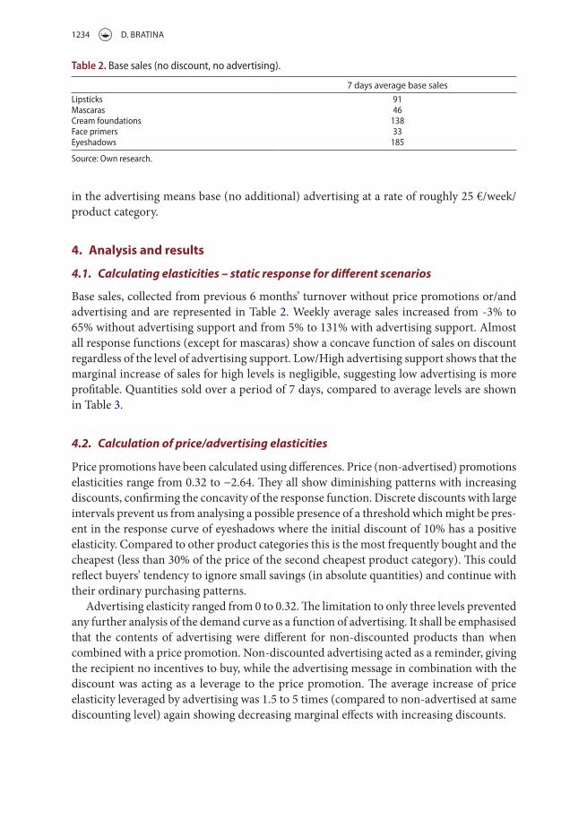
Base sales, collected from previous 6 months’ turnover without price promotions or/and advertising and are represented in Table 2. Weekly average sales increased from -3% to 65% without advertising support and from 5% to 131% with advertising support. Almost all response functions (except for mascaras) show a concave function of sales on discount regardless of the level of advertising support. Low/High advertising support shows that the marginal increase of sales for high levels is negligible, suggesting low advertising is more profitable. Quantities sold over a period of 7 days, compared to average levels are shown in Table 3.

4.2. Calculation of price/advertising elasticities

Price promotions have been calculated using differences. Price (non-advertised) promotions elasticities range from 0.32 to −2.64. They all show diminishing patterns with increasing discounts, confirming the concavity of the response function. Discrete discounts with large intervals prevent us from analysing a possible presence of a threshold which might be pres-ent in the response curve of eyeshadows where the initial discount of 10% has a positive elasticity. Compared to other product categories this is the most frequently bought and the cheapest (less than 30% of the price of the second cheapest product category). This could reflect buyers’ tendency to ignore small savings (in absolute quantities) and continue with their ordinary purchasing patterns.

Advertising elasticity ranged from 0 to 0.32. The limitation to only three levels prevented any further analysis of the demand curve as a function of advertising. It shall be emphasised that the contents of advertising were different for non-discounted products than when combined with a price promotion. Non-discounted advertising acted as a reminder, giving the recipient no incentives to buy, while the advertising message in combination with the discount was acting as a leverage to the price promotion. The average increase of price elasticity leveraged by advertising was 1.5 to 5 times (compared to non-advertised at same discounting level) again showing decreasing marginal effects with increasing discounts.

Table 2. Base sales (no discount, no advertising).

source: own research.

7 days average base salesLipsticks 91mascaras 46cream foundations 138Face primers 33Eyeshadows 185

ECONOMIC RESEARCH-EKONOMSKA ISTRAŽIVANJA 1235

Tabl

e 3.

 incr

ease

in sa

les f

or d

iffer

ent s

ettin

gs o

f adv

ertis

ing

and

pric

e.

sour

ce: o

wn

rese

arch

.

% d

isco

unt

0%10

%20

%30

%40

%50

%

Leve

l of a

dver

tisin

gba

selo

whi

ghba

seba

selo

whi

ghba

selo

whi

ghba

selo

whi

ghba

selo

whi

ghLi

pstic

ks0%

21.3

%15

.6%

1.5%

−1.

8%39

.7%

46.7

%49

.5%

41.0

%45

.4%

53.3

%90

.8%

mas

cara

s0%

12.7

%19

.2%

16.2

%16

.2%

19.2

%21

.7%

23.7

%cr

eam

foun

datio

ns0%

19.0

%17

.1%

11.2

%19

.2%

23.0

%25

.5%

28.6

%37

.9%

39.1

%41

.1%

39.4

%52

.4%

53.2

%Fa

ce p

rimer

s0%

17.1

%19

.1%

0.0%

19.4

%21

.0%

23.3

%25

.7%

31.4

%34

.4%

37.1

%40

.0%

47.1

%47

.3%

Eyes

hado

ws

0%2.

9%5.

1%−

3.0%

32.7

%49

.0%

53.7

%59

.2%

60.9

%95

.2%

123.

2%13

1.8%

1236 D. BRATINA

4.3. In search for persistence of marketing activities: dynamic modelling

In the second part of our research we turned our attention to the study of lagged effects of price promotions/advertising and the combination of both, by analysing the 5 aggregated product categories’ daily sales and page views time series. Figure 1 shows an extract from the lipsticks product category web page view time series.

Each setup ran for 7 days before returning to no marketing activity for at least 14 days. To account for all combinations of advertising and discounts, aggregated (all SKUs of a product category together) time series have been used throughout the entire period of the experiment (7 months) and joined with pre-and post-experimental periods of 2 months for a total of 11 months. All marketing efforts had a step function shape that can be modelled as:

and combined with the best AIC ARIMA model. Tables 4 and 5 shows best fitted ARIMAX model for page views and purchases of time series prior to the research.

(7)P(T)t =

{

1, if t = T

0, otherwise,

Figure 1. Lipsticks page views during advertising campaign. source: own research.

Table 4. Page clicks aic.

source: own research.

Page-clicks A.R.I.M.A. model 1 day AIC.(1,0,0)(1,0,0)7 1418(0,0,1)(0,0,1)7 1512(1,0,1)(1,0,1)7 1386(1,1,1)(1,1,1)7 1270(2,0,0)(2,0,0)7 5520

ECONOMIC RESEARCH-EKONOMSKA ISTRAŽIVANJA 1237

Both series follow a pattern of (1,1,1)(1,1,1)7 showing a 7 days seasonality, which was expected in daily sales time series. More important is the shape of the two exogeneous variable functions. According to (van Heerde et al., 2000), (Heerde et al., 2002) and (Cryer & Chan, 2015), a diminishing effect intervention has a functional form:

when immediate and

when lagged, where ω represents the increased effect, δ the decay, and B is the lag operator. If sales response follows an immediate response with decreasing effect without lags the functional form should be as in Equation 8. The term �0

1−�1BP(T) can be developed as Taylor

series into (ω0+�0�1B + �0�21B

2 +…+)P(T) and is convergent for ω1B < 1. For advertising a lagged effect is thus expected to have a functional form of �2B

1−�3BP(T), developed in series

as (�2B + �2�3B2 + �2�

23B

3 +…+)P(T) . On day t = T of marketing activity we thus get ω0 as sales response, and ω1BP(T) = ω10 = 0 as advertising response if the above holds true. Day t = T+1 sales are (ω0ω1B)P(T)=�0�1 and advertising response is ω2. As �1,�2and ω3 < 0 we get an exponential decay after the initial effect of ω1 for sales occurring at time t and ω2effect of advertising occurring at time t+1.

Table 6 shows the regression coefficients for all five-time series, where the regression equation used was:

(8)�0

1 − �1BP(T),

(9)�2B

1 − �3BP(T),

(10)(1 − B)(

1 − B7)

Yt = � + �ATt +

�0

1 − �1BPTt +

�2B

1 − �3BAT

t + (1 − B)(

1 − B7)

wt + e ,

Table 5. Purchases aic.

source: own research.

Purchases ARIMA model 1 day AIC(1,0,0)(1,0,0)7 633(0,0,1)(0,0,1)7 624(1,0,1)(1,0,1)7 591(1,1,1)(1,1,1)7 562(2,0,0)(2,0,0)7 612

Table 6. Regression coefficients.

*= sig < 0.05.;**= sig < 0.01.;source: own research.

Series (category) θ (AR) θ (MA) θs (SAR) θ (SMA) ω0 δ ω1 ω2 ω3

Lipsticks 0.12** 0.74** −0.15** −0.64** 12* 1.05 0.57* 6.2* 0.11**Foundations 0.22** 0.91* −0.27** −0.23** 24** 0.2 0.83* 8.4* 0.22**mascara 0.18** 0.79** −0.45* −0.54* 17 −0.5 0.26** 9.1* 0.15**Primer 0.14** 0.51* −0.54* −0.34* 22** −1.5 0.26** 12.6* 0.22**Eyeshadows 0.15** 0.91** −0.66* −0.25* 50** 1.3 0.35* 21.2* 0.13**

1238 D. BRATINA

where the term �0PTt . and �AT

t are the immediate effects of advertising at time T, the ω2B is the lagged effect of advertising at T+1, the term 1

1−�3B. its decay. Other terms represent

factors of ARIMA (1,1,1)(1,1,1)7 model.All coefficients except delta are statistically significant, suggesting that sales and adver-

tising shapes could be of anticipated form with sales having an immediate effect of around 30 items/day, while advertising effects starts at second day and is also decaying and more rapidly (ω1vs ω3). The effect of advertising is also much less significant than advertising. While one would expect an increasing advertising effect as per (Heerde et al., 2002) and many others, our findings are in fact not in contradiction with their findings, as advertising is more of a sales support than other marketing-communications means.

5. Further research

Our assumption of the functional form of the response functions are based on subjective assumptions and need further research. Using transfer function analysis, one could easily test other types of functionalities and choose the best model for use. The limitations of such analysis are however in the fact that the magnitude of the effect is not considered. One would have to balance complexity (VARIMAX) and speed (ARIMAX) and consider data availability when deciding which time-series analysis to use. The digital analytics tools today allow us to increase the time resolution of our research to perhaps hours (instead of days or weeks) where the purchase quantities are high enough. This way one could get insight to the information build up and decay in almost real time.

Marginal effects diminish with increasing effort, but how does time length affect the deal curve? An experiment, adding different lengths to the existing various setups of discounts and advertising levels would provide information about how long an effort should be run-ning (should a company use short bursts of activities or longer ones). More exogenous variables such as consumer demographics and psychographic characteristics would surely give better forecasting power at the expense of cost and time.

Disclosure statement

No potential conflict of interest was reported by the author.

References

Assmus, G., Farley, J. U., & Lehmann, D. R. (1984). How advertising affects sales: A meta analysis of econometric results. Journal of Marketing Research, 21(1), 65–74.

Box, G. E. P., & Tiao, C. (1975). Intervention analysis with applications to economic and enviromental problems. Journal of the American Statistical Association, 70(March), 70–79.

Broadbent, T. (1999, November). What’s the use of tracking studies? Admap, 18–20.Cryer, D., & Chan, K.-S. (2015). Time series analysis with applications in R. New York, NY: Springer.Datoo, B. A. (2017). American marketing association. Retrieved from https://archive.ama.org/archive/

ResourceLibrary/MarketingResearch/documents/9511240224.pdfDekimpe, M., & Hannsens, D. (1995). Empirical generalizations about market evolution and

stationarity. Marketing Science, G109–G121.Dickey, D. A., Hazsa, D. P., & Fuller, W. A. (1984). Testing for unit roots in seasonal time series.

Journal of the American Statistical Asosciation, 79, 355–367.Doyle, P., & Saunders, J. (1985). The lead effect in marketing. Journal of Marketing Research, 22, 54–76.

ECONOMIC RESEARCH-EKONOMSKA ISTRAŽIVANJA 1239

Franses, P. H. (1991). Primary demand for beer in the Netherlands: An application of ARMAX model specification. Journal of Marketing Research, 28(2), 240–245.

Hannsens, D. M., Parsons, L. J., & Schultz, R. L. (2001). Market response models – Econometric and time series analysis. Boston, MA: Kluwer Academic Publishers.

Heerde, H. J., Wittink, D. R., & Leeflang, P. S. (2002). Flexible decomposition of price promotion effects using store-level scanner data. Cambridge, MA: Marketin Science Institute.

Heerde, H. J., Leeflang, P. S., & Wittink, D. R. (2000). The Estimation of pre- and post- promotion dips with store-level scanner data. Journal of Marketing Research, 37(3), 383–395.

Krugman, H. E. (1972). Why three exposures may be enough. Journal of Advertising Research, 6, 11–14.

Leone, R. P. (1995). Generalizing what is known about temporal aggregation and advertising carryover. Marketing Science, 14(3), G141–G150.

Lodish, L. M., & Lubetkin, B. (1992, February). How advertising works. General truths? None key findings from IRI test data. Admap, 9–15.

McDonalds, C. (1995, February). Where to look for the most trustworthy evidencce. Short-ter advertising effects are the key. Admap, 25(7).

Morey, R. C., & McCann, J. M. (1983). Estimating the confidence interval for the optimal marketing mix: An application of lead Generation. Marketing Science, 7–13, 193–202.

Roberts, A. (1999, Februrary). Recency, frequency and the sales effects on TV advertising. Admap, 40–44.

Sethuraman, R., & Tellis, G. (1991). An analysis of the tradeoff between advertising and pricing. Journal of Marketing Research, 31, 160–174.

Simon, J. (1979). What do Zielske’s real data swow about pulsing? Journal of Marketing Research, 16, 415–420.

Simon, J., & Arndt, J. (1980). The shape of the advertising response function. Journal of Advertising research, 20(4), 11–28.

Tellis, G. (1989). Interpreting advertising and price elasticities. Journal of Advertising Research, 29(4), 40–43.

Tellis, G. J. (2006). Medlling marketing mix. In R. Grover, Handbook of marketing research (pp. 506–522). Thousand Oaks: Sage Publications.

Vakratsas, D., Feinberg, F., & Kalyanaram, G. (2004). The shape of advertising response function revisited: A Modle of Dynamic Probabilistic Thresholds. Marketing Science, 23(1), 109–119.

Van Heerde, H. J., Leefland, P. S., & Wittink, D. R. (2001). Semi parametric analysis to estimate the deal effect curve. Journal of Marketing, 37, 197–215.

Wichern, D. W., & Jones, R. H. (1977). Assessing the impact of market disturbances using intervention analysis. Management Science, 24(3), 329–337.