ELDERLY PROSPERITY AND HOMEOWNERSHIP IN THE EUROPEAN UNION: NEW

EVIDENCE FROM THE SHARE DATA

Stijn Lefebure Joris Mangeleer

Karel Van Den Bosch

Discussant Commentsby Edward N. wolff

August 2006

Summary of Paper

• 1. Elderly population often combines low household income with high home ownership rates.

• 2. Adding a rate of return to home values singnificantly reduces the poverty rate of the elderly, particulalry in Southern and Central Europe.

• 3. The authors take home equity into account in three ways:

Summary (continued)

• (i) Simulating a reverse mortgage.

• (ii) Moving to a smaller dwelling

• (iii) Adding imputed rent to income

• 4. Big reduction in poverty rates when home equity is converted into income.

• 5. Also, inequality among elderly declines substantially if home equity is converted to consumption.

Detailed Findings

• 1. Primary analysis uses SHARE database for 15 EU countries.

• 2. Figure 1: Poverty in the European Union (EU15) by age groups, 2003. Poverty line 60% of median national equivalent income In 2003, 13 of the 15 countries of the former EU15 recorded a higher poverty risk for the over-65s than for the under-65s (Italy and Netherlands the exception). In the Scandinavian countries, poverty rates among the elderly are between 15% and 17%; in Ireland, Portugal, and Greece, over 25%; in UK, about 25%. [In US, elderly poverty rates lower than under-65]..

•

Detailed Findings (cont.)

• 3. Table 1: In many countries, more homeowners than non-home owners among elderly poor (Spain, Italy, and notably Greece). In other countries, large share of homeowners among elderly poor.

• 4. In SHARE dataset, housing wealth (not usre if net or gross?) accounts for 54-86% of total household wealth. [In US, gross housing: 28% in 2001, 33% in 2004 for all households].

Detailed findings (continued)

• 5. In actuality, housing mobility among elderly is very limited (the elderly do not change residence very often). Indeed, elderly often move to larger homes. Reverse mortgages where they exist (US, France, UK) very limited in usage.

• 6. Poverty rate in SHARE dataset set at income level that matches poverty rate for elderly in SILC.

Detailed Finding (continued)• 7. Table 4: Poverty among elderly homeowners before and after

home equity conversion • Base income Imputed rent Moving Rev. Mortgage • Austria 15% 7% 5% 5% • Germany 14% 4% 5% 4% • Sweden 10% 7% 5% 5% • Netherlands 9% 1% 3% 1% • Spain 32% 7% 11% 6% • Italy 18% 4% 6% 4% • France 13% 5% 5% 3% • Denmark 13% 3% 5% 2% • Greece 29% 12% 15% 8%

Detailed Findings (cont.)• 8. Table 5: Atkinson (0.5) inequality indices before and after

home equity conversion Base Imputed rent Sale+Buy Rev. mortgage

• Austria 0.177 0.168* 0.172 0.167* • Germany 0.125 0.124* 0.130 0.122* • Netherlands 0.181 0.162* 0.165* 0.159* • France 0.183 0.173 0.164* 0.156* • Denmark 0.113 0.118 0.124 0.109 • Sweden 0.114 0.113 0.122 0.110 • Greece 0.126 0.119* 0.135 0.113* • Spain 0.153 0.124* 0.138* 0.118* • Italy 0.165 0.152* 0.166 0.153* • Within group 0.154 0.145 0.150 0.139 • Bet. group 0.025 0.020* 0.015* 0.017*

Comments I

• 1. Imputed rent is computed as a fixed percentage (4%) of net home value (figures are provided in SHARE). Are the household imputed rent figures align to NIPA totals?

• 2. In these simulations, poverty line is unchanged. Maybe poverty line should also be changed.

• 3. Similar findings on imputed rent and elderly poverty reported by Wolff (1990): "Wealth Holdings and Poverty Status in the United States," Review of Income and Wealth, Series 36, No. 2, June, 1990, 143-65.

Comments II

• 4. What equivalence class is used for median national equivalent income?

• 5. Annuity calculation in footnote 8: Not usre that it will exhaust asset value by end of life expectancy. Is this true? Text says interest rate is set at 5% but footnote 8 indicates it is 4%.

• 6. In “Moving” scenario, how are proceeds from sales allocated to income? If “annuity” how is the mortgage on the original house treated?

Comments III

• 7. Inequality differences are relatively small after conversion of housing equity.

• 8. Why don’t the elderly run down the value of their homes? (i) uncertainty about time of death. (ii) Bequest motive. (iii) Why not sell house and rent it back from, say, children?

“The Evolution of Private Pensions, the Effects

of Aging, and the Variance in Assets”

Joseph T. Marchand

Discussant RemarksEdward N. Wolff

August 2006

Summary of Findings

• 1. The variance in assets of a given cohort is predicted to increase as a cohort ages.

• 2. Marchand finds that the variance in total assets increases at 1.3% per year.

• 3. The variance in financial and non-financial assets increases at less than 1% per year.

Summary (continued)

• 4. A 1% increase in percent that hold DB plans decreases variance of assets by 0.7 percent.

• 5. A 1% increase in percentage of DC holders increases variance in assets by 0.8%.

Detailed Findings

• 1. Deaton (1992) and Deaton, Gourinchas, and Paxson (2002) show theoretically that inequality in assets will be higher when there is more individual risk among a cohort of individuals.

• 2. Since 1980, considerable change in US pension system, with substantial decline in traditional DB plans and corresponding increase in DC plans.

Detailed Findings (cont.)

• 3. Amount of DB plans declined from 87% in 1983 to 44% in 1998, while DC plans increased from 40 to 79%. [Not sure what “amount” means – the total value or the number of holders?]

• 4. [I also discuss transformation in: “The Devolution of the American Pension System: Who Gained and Who Lost?” Eastern Economics Journal. Vol. 29, No. 4, Fall 2003, pp. 477-495].

Detailed Finding (cont.)

• 5. On page 8: “However, none of these studies specifically looked at the consequences of shifting risk on the variance of assets.” But my study looks precisely at rising inequality of pension wealth and total wealth from the shift in the pension system.

• 6. Intertemporal Choice Model [skip on account of time limitations].

Detailed Findings (cont.)

• 7. Uses HRS (individuals over age 50). Four cohort samples: (1) HRS, born 1931-1941. (2) AHEAD, born before 1924. (3) War Baby (WB), born 1942-1947. (4) CODA (depression-era kids), born 1924-1930.

• 8. Figure 1 clearly shows a stat. significant upward trend over time in Var(Log(Assets)) for each cohort.

Detailed Findings (cont.)

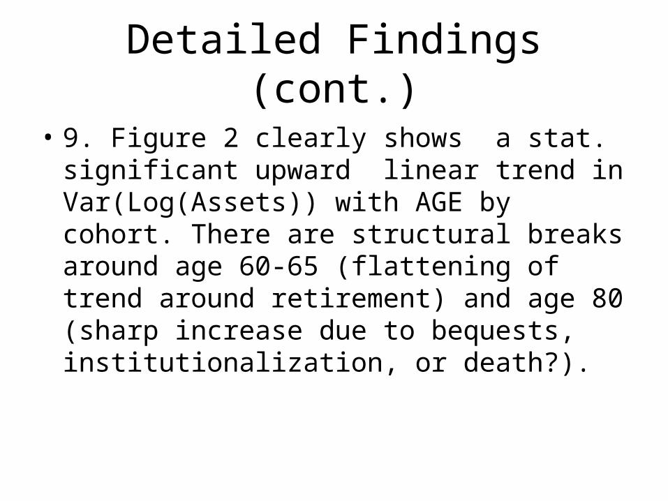
• 9. Figure 2 clearly shows a stat. significant upward linear trend in Var(Log(Assets)) with AGE by cohort. There are structural breaks around age 60-65 (flattening of trend around retirement) and age 80 (sharp increase due to bequests, institutionalization, or death?).

Detailed Findings (cont.)

• 10. Estimate:• (45) Var(Log(Assets) = a +

b*Share(DBAssets) • (46) Var(Log(Assets) = a +

b*Share(DCAssets)• where industry-year observations are used

as the exogenous variation. Industry share with DB or DC based on self-reported responses.

Detailed Finding (cont.)

• 11. Results for variance of total assets:• Table 2. Variance of the Logarithm of Assets on

Percentage of DB Holders • OLS Regression Results by Asset Classes Using

Unmasked Industries • Total Linear Fit Elasticity • Assets (n=364) (1) (2) (3) (4) • % of DB Holders -0.010 -0.009 -0.007 -0.006

– (0.003) (0.003) (0.001) (0.002) – [0.000] [0.001] [0.000] [0.000]

• year dummies X X • R-squared 0.04 0.07 0.07 0.10

Detailed Findings (cont.)

• Table 3. Variance of the Logarithm of Assets on Percentage of DC Holders

• OLS Regression Results by Asset Classes Using Unmasked Industries

• Total Linear Fit Elasticity • Assets (n=364) (1) (2) (3) (4) • % of DC Holders 0.011 0.010 0.008 0.007 • (0.002) (0.002) (0.001) (0.001) • [0.000] [0.000] [0.000] [0.000] • year dummies X X • R-squared 0.05 0.08 0.08 0.11

Comments I

• 1. The model: (i) Why is r fixed over time? (ii) Relatedly, in equation (9), the change of assets equals (1+r) times savings. But what about capital gains and the revaluation of existing assets? (iii) why is the variance of earnings assumed fixed?

• 2. Why look at the variance of assets? What about debt and net worth? Why are we interested just in assets and asset variance?

Comments II

• 3. Why separate out financial from non-financial assets? Is there a theoretical rationale for this? Aren’t the two types of assets fungible -- particulalry if you include debt so that people can borrow against one kind of assets (say housing) to purchase another kind of assets (say stocks).

Comments III

• 4. A little confused about estimation industry for share(DB) and share(DC). Why use industry-year observations as the exogenous variation rather than, say, age-year observations or even occupation-year. Also, how do you know industry for the retired?