•electe - defense technical information center not reflect the official policy or position of the...
TRANSCRIPT

L_ )
-Va
ANALYTICAL MODELING OF AQUIFERDECONTAMINATION BY PULSED PUMPING WHEN
CONTAMINANT TRANSPORT IS AFFECTED BYRATE-LIMITED SORPTION AND DESORPTION
THESIS
Thomas A. Adams, Captain, USAFRobert C. Viramontes, Captain, USAF
AFIT/GEE/ENC/93-Si .1
•ELECTE r
S,%~' "a DEPARTMENT OF THE AIR FORCEAIR UNIVERSITY
AIR FORCE INSTITUTE OF TECHNOLOGY
Wright-Patterson Air Force Base, Ohio

AFIT/GZ/ENC/193-Si
ANALYTICAL MODELING OF AQUIFERDECONTAMINATION BY PULSED PUMPING WHEN
CONTAMINANT TRANSPORT IS AFFECTED BYRATE-LIMITED SORPTION AND DESORPTION
THESIS
Thomas A. Adams, Captain, USAFRobert C. Viramontes, Captain, USAF
AFIT/GEE/ENC/93-Si
Approved for public release; distributi.,n unlimited
93-23991 @j ~ I4' 5 1111)u.

The views expressed in this thesis are those of the authors anddo not reflect the official policy or position of the Departmentof Defense or the U.S. Government.
ooeuion For
NTIS GRA&IDTIC TAB 0Unannounced I-3Justification
.. 'By- •Distribution/
~~ Availability CAOR.
Nat Special

ArIT/GEZEZNC/193-Si
ANALYTICAL MODELING OF AQUIFER DECONTAMINATION BY PULSED PUMPING
WHEN CONTAMINANT TRANSPORT IS AFFECTED BY
RATE-LIMITED SORPTION AND DESORPTION
THESIS
Presented to the Faculty of the School of Engineering
of the Air Force Institute of Technology
Air Education and Training Command
In Partial Fulfillment of the
Requirements for the Degree of
Master of Science in Engineering and Environmental Management
Thomas A. Adams, B.M.E. Robert C. Viramontes, B.S.M.E.
Captain, USAF Captain, USAF
September 1993
Approved for public release; distribution unlimited

Acknowledgments
We are extremely grateful to all of the people involved in
making this thesis possible. We hope our research efforts in
the field of contaminant transport modeling will contribute
additional insight into studying this complex phenomena.
We are greatly indebted to our faculty advisor, Dr Mark E.
Oxley, who without his guidance, infinite patience, and
countless hours reviewing various concepts and mathematical
theories with us this thesis would not have become a reality.
We also wish to extend our deepest appreciation to our
committee members during this undertaking. For helping us to
understand the groundwater concepts and physics and for
providing numerous articles and FORTRAN programs, we thank
Lieutenant Colonel Mark N. Goltz. His expertise definitely
helped us make the transition from the physical world to the
mathematical and numerical worlds much easier. Additionally, we
thank Major Dave L. Coulliette for his professional assistance
with the numerical analysis and evaluation and for listening to
all of our problems throughout the development of this thesis.
A word of appreciation is also due to Lieutenant Colonel
William P. Baker who provided encouragement during times of
frustration and for his assistance with the mathematical
analysis. His collaboration was more than welcomed.
Finally, our most heartfelt thanks must go to our wives,
Jennifer Adams and Mary Viramontes, and families. This thesis
has taken an enormous amount of time and without the love and
ii
endless patience with which our wives have supported this
research, we could have never endured its demands. We owe them
a lifetime of gratitude. A special thanks to Adam, Erin, and
Ryan Viramontes who can now reap the benefits of having their
Dad back into a more 'active' role. A special thanks also to
Christine Adams who has patiently, lovingly, and obediently
helped her parents through these past 15 months which included
the turbulent births of her brothers Matthew and Nicholas.
Above all else, we thank God for the grace he has given us
to not only survive but to excel in these difficult but
rewarding times. Without Him, we can do nothing.
Thomas A. Adams
Robert C. Viramontes
iii

Table of Contents
Page
Acknowledgments ................................ ii
List of Figures ................................ vi
List of Tables.................. vii
List of Symbols ................................ viii
Abstract.................... xi
I. Introduction .............................. 1-i
Background .i.......................... 1-1Specific Problem. ..................... 1-5Research Objectives .................... 1-6Scope and Limitations. .................. 1-7Definitions .......................... 1-8Overview. ........................... 1-9
II. Literature Review .......................... 2-1
Overview. ........... .............. 2-1Contaminant Transport Processes ........... 2-4
Mass Transport .................... 2-4Mass Transfer. .................... 2-6
Advection-Dispersion-Sorption Models . . 2-7Sorption Equilibrium ............... 2-10Sorption Nonequilibrium ............. 2-12
Chemical .................... 2-13Physical .................... 2-13
First-Order Rate .......... 2-14Fickian Diffusion ......... 2-16
Pulsed Pumping ........................ 2-18Summary ............................. 2-21
III. Model Formulation .......................... 3-1
Introduction ................. .. 3-1Model Assumptions and Aquifer Characteristics 3-1Governing Equations and Solutions ......... 3-4
Model Formulation: Extraction Well On . 3-5Initial Conditions . ............ 3-10Boundary Conditions ............ 3-11Laplace Transform ............. 3-12
Laplace Solution. ......... 3-13Green's Function. ......... 3-15
iv

Model Formulation: Extraction Well Off . 3-21Laplace Solution ............ .. 3-23Green's Function. ............. 3-25
IV. Analysis and Evaluation of Results ............. 4-1
Numerical Evaluation ................... 4-1Laplace Inversion ................. 4-2Gauss-Quadrature Integration ......... 4-3Cubic-Spline Interpolation . .......... 4-4Numerical Difficulties. . ...... 4-4
Model Simulations 4-5Pulse versus Continuous Pumping . . . 4-7
Efficiency Comparison. .......... 4-16Continuous Pumping . ................ 4-19
Model Verification/Comparison . ............ 4-22
V. Conclusion and Recommendations. ................ 5-1
Overview ............................ 5-1Summary of Findings .................... 5-2Recommendations............. 5-4
Appendix A: A Green's Function Approach to AnalyticalModeling Aquifer Decontamination by PulsedPumping With Arbitrary Initial Conditions . A-I
Appendix B: Flowchart . .......................... B-I
Appendix C: Source Code ......................... C-I
Bibliography... ...... .... ................. . .. BIB-I
Vitas............. ....................... .... VITA-I
V

List of Figures
Figure Page
2.1. Effluent Concentration Pattern for ContinuousWellfield Operations ....................... 2-1
2.2. Potential Groundwater Contamination Response toCessation of Continuous Pumping ............... 2-3
2.3 Conceptualization of Aquifer Remediation, WhereContaminant Transfer May Be Affected by Rate-LimitingMechanisms . .............................. 2-17
2.4 Potential Effluent Concentration for Pulsed PumpingRemediation .............................. 2-20
4.1 10-Point Gauss-Quadrature Sampling of I0 (x). . . . 4-6
4.2 Pulsed Pumping Effluent Concentration Profile WhenSorption/Desorption is Controlled by DiffusionWithin Layers. ............................ 4-9
4.3 Continuous Pumping Effluent Concentration ProfileWhen Sorption/Desorption is Controlled by DiffusionWithin Layers. ............................ 4-10
4.4 Effluent Concentration Profile for Pulsed VersusContinuous Pumping Comparison at the Well WhenSorption/Desorption is Controlled by DiffusionWithin Layers. ............................ 4-11
4.5 Efficiency Comparison: Pulsed Versus ContinuousPumping ................................. 4-17
4.6 Mass Removed Versus Volume of Water Extracted:Pulsed Versus Continuous Pumping. ............. 4-18
4.7 Initial Conditions for Continuous Pumping Simulation 4-20
4.8 Continuous Pumping Effluent Concentration ProfileUsing Arbitrary Initial Conditions for the LayeredDiffusion Model ........................... 4-21
4.9 Continuous Pumping Effluent Concentration ProfileUsing Arbitrary Initial Conditions for the LayeredDiffusion Model (first 10 days) ............... 4-23
4.10 Effluent Concentration Profile Comparison at theWell When Sorption/Desorption is Controlled byDiffusion Within Layered Immobile Regions . . . . 4-26
Vi

List of Tables
Table Page4.1. Input Parameters for the Layered Diffusion
Simulation . .............................. 4-7
4.2. Mobile Concentration Comparison at the Well . . . 4-8
4.3. Immobile Region Concentration Comparison (PulsedVersus Continuous Pumping at the Well-at day 100. 4-12
4.4. Immobile Region Concentration Comparison (PulsedVersus Continuous Pumping at the Well-at day 200. 4-13
4.5. Immobile Region Concentration Comparisoi, (PulsedVersus Continuous Pumping at the Well-at day 300. 4-14
4.6. Immobile Region Concentration Comparison (PulsedVersus Continuous Pumping at the Well-at day 400. 4-15
4.7. Mobile Concentration Profile for the First 10 Days 4-22
4.8. Layered Mobile Region Comparison Test . .......... 4-26
vii

List of Symbols
a Immobile region radius or half width [L]
at Longitudinal dispersivity [hL
b Aquifer thickness [L]
C(r,t) Contaminant aqueous concentration [M / 52]
C"(r,z,t) Local solute concentration at points within the
immobile region [M I 12]
C.(X, Z,T) Dimensionless concentration at points within theimmobile region
C.(X, Z,s) Dimensionless Laplace transformed concentration atpoints within the immobile region
C'(r,t) Volume-averaged immobile region solute concentration
[M / L1]
CQ(X,T) Dimensionless volume-averaged immobile region soluteconcentration
C.(X,S) Dimensionless Laplace transformed volume-averagedimmobile region solute concentration
C'(r,t) Solute concentration in the mobile region [M / 51]
Cm(XT) Dimensionless mobile region solute concentration
Cm(XS) Dimensionless Laplace transformed mobile regionsolute concentration
C" Initial maximum concentration in the mobile and
immobile region [M / L2]
viii

D. Mobile region dispersion coefficient [L2 / T]
UP Immobile region solute diffusion coefficient [L! / T]
D. Dimensionless immobile region solute diffusioncoefficient
Do Mobile region molecular diffusion coefficient [L2 / T]
F'(r) Initial solute concentration in the mobile region
[M /L0]
Fm(X) Dimensionless initial solute concentration in themobile region
F'(r) Volume-averaged initial solute concentration in the
immobile region [M / L3]
Fý(X) Dimensionless volume-averaged initial soluteconcentration in the immobile region
F'(r, z) Initial local solute concentration at points within
the immobile region of a certain geometry [M / 5?]
F.(X, Z) Dimensionless initial solute concentration in theimmobile region of a certain geometry
Kd Mobile region distribution coefficient [19 / M]
Q, Extraction well pumping rate [L? / T]
Rim Immobile region retardation factor
Rm Mobile region retardation factor
r Radial distance variable [L]
ix

Extraction well radius [L]
Radius of initially contaminated zone [U]
S Laplace transform variable
S(r,t) Sorbed contaminant or sorbed solute concentration
t Time variable [T]
T Dimensionless time variable
V(r) Mobile region seepage velocity [L / T]
Vm Same as V(r) [L / T]
X Dimensionless radial distance variable
Xw Dimensionless extraction well radius
X. Dimensionless radius of initially contaminated zone
Z Variable used within the immobile region [U]
Z Dimensionless immobile region variable
a First-order rate constant [T-i]
c Dimensionless first-order rate constant
P Solute capacity ratio of immobile to mobile regions
£ Coefficient of leakage of the solute from thecontaminated zone to the outer boundary
0 Total aquifer porosity or water content
Om Mobile region water content
0. Immobile region water content
p Bulk density of aquifer material [M / 12]
x

AFIT/GEE/ENC/93-SI
Abstract
This research explores radially convergent contaminant
transport in an aquifer towards an extraction well. This thesis
presents the equations governing the transport of a contaminant
during aquifer remediation by pulsed pumping. Contaminant
transport is assumed to be affected by radial advection,
dispersion, and sorption/desorption. Sorption is assumed to be
either equilibrium or rate-limited, with the rate-limitation
described by either a first-order law, or by Fickian dif :usion
of contaminant through layered, cylindrical, or spherical
immobile water regions. The equations are derived using an
arbitrary initial distribution of contaminant in both the mobile
and immobile regions, and they are analytically solved in the
Laplace domain using a Green's function solution. The Laplace
solution is then converted to a formula translation (FORTRAN)
source code and numerically inverted back to the time domain.
The resulting model is tested against another analytical Laplace
transform model and a numerical finite element and finite
difference model. Model simulations are used to show how pulsed
pumping operations can improve the efficiency of contaminated
aquifer pump-and-treat remediation activities.
xi

ANALYTICAL MODELING OF AQUIFER DECONTAMINATION BY PULSED
PUMPING WHEN CONTAMINANT TRANSPORT IS AFFECTED
BY RATE-LIMITED SORPTION AND DESORPTION
IgIntroduction
Groundwater is the source of drinking water for
approximately 48,000 communities and twelve million individuals
across the country. Almost all rural households and thirty-four
of the nation's 100 largest cities depend upon groundwater as
their drinking water source [Wentz, 1989:271] . Historically,
groundwater has been considered an unlimited and safe source of
drinking water. However, the widespread contamination of
groundwater due to years of accidental or deliberate dumping of
various synthetic organic chemicals is becoming an issue of
growing importance in the United States. Many of these
chemicals are known or potential carcinogens or teratogens and
their presence in the groundwater, even at low concentrations,
presents serious and substantial health risks [Chiras, 1991:388;
Wentz, 1989:270].
It has been estimated that "more than 70 percent of the
nearly 1,200 hazardous-waste sites on the Superfund National
Priorities List (NPL) are contaminated with chemicals at levels
exceeding federal drinking-water standards" [National,
1-1

1991:117]. In addition, over 33,000 other sites have been
identified and included in the Comprehensive Environmental
Response, Compensation, and Liability Information System for
ranking and potential inclusion on the NPL. Furthermore.
groundwater contamination has been identified or is suspected at
more than 1,700 Resource Conservation and Recovery Act
facilities. These sites constitute an immense groundwater
contamination problem [Olsen and Kavanaugh, 1993:42]. In
response, the Air Force is engaged in a program to identify,
assess, and remediate hazardous waste sites at military
installations throughout the United States [Goltz, 1991:24;
Installation Restoration Program Handout, 1992]. This program
is known as the Installation Restoration Program (IRP).
IRP cleanups will cost the Air Force an estimated $7-10
billion over the next ten years [Vest, 1992]. A substantial
portion of IRP costs is associated with groundwater
contamination remediation. Consequently, site remediations
often include aquifer cleanup efforts. Because of the rising
cost to perform aquifer remediation, it is critical that
decisions made regarding groundwater cleanup be based upon the
best available information. One major source of information
provided to IRP decision makers comes from contaminant transport
models [Goltz, 1991:24].
Contaminant transport modeling plays an important part in
aquifer remediation. These mathematical models are used as
tools for predicting trends over short or long term periods by
1-2
simulating the effects of various processes occurring
simultaneously in an aquifer that can affect the transport or
concentration of pollutants [Ismail, 1987:274]. The knowledge
gained using these models can be applied by IRP planners to
determine the effectiveness of various groundwater treatment
technologies, estimate risk, and make predictions about the cost
and duration of cleanup efforts [Goltz, 1991:24]. One problem
with these models involves assumptions that are made to simulate
the chemical, biological, or physical processes that are
occurring in the aquifer [Goltz, 1991:24]. Model simulations
may significantly differ from reality, depending on actual site
conditions.
One assumption commonly made when modeling organic
contaminant transport is the local equilibrium assumption (LEA)
[Goltz, 1991:24]. The LEA is one method used to describe the
relationship between the amount of contaminant that is sorbed to
soil particles in the aquifer and the amount dissolved in the
water (aqueous). Under the LEA, a retardation factor is used to
account for the sorption of the contaminant to the soil. The
use of this retardation factor implies an instantaneous
equilibration between the aqueous and sorbed contaminant [Goltz,
1991:24]. Thus, the LEA assumes the contaminant sorbed to the
soil particles is instantaneously desorbed into the clean water
as an extraction pump extracts contaminated water and clean
water flows in to replace it [Goltz, 1991:24] . Since organic
contamination is a main concern at Air Force installations, the
1-3

LEA is often used to model contaminant fa~e and transport at Air
Force IRP sites [Goltz, 1991:24]. However, the occurrence of
two phenomena in several laboratory and field studies suggests
the LEA is often not a valid assumption [Goltz, 1991:24; Goltz
and Roberts, 1988; Brusseau and Rao, 1989:41; Weber and others,
1991:505].
The first phenomenon is termed 'tailing', and it is used to
describe the asymptotic decrease in the rate of reduction of
contaminant concentration in extracted water after a relatively
rapid initial decrease. The second phenomenon, termed
'rebound', involves the increase in contaminant concentration
that is observed after cessation of pumping. Oftentimes, this
behavior is observed several years after the pump or pumps have
been stopped and the hazardous site closed [Goltz, 1991:25;
Valocchi, 1986; EPA 600/8-90/003, 1990:14; Keely and others,
1987:91: Travis and Doty, 1990:1465; Mackay and Cherry,
1989:633]. Under these conditions, it appears that contaminant
in the sorbed -.-id aqueous phases does not instantaneously
equilibrate but only slouly reaches equilibrium [Goltz and
Oxley, 1991:547]. This rate-limited sorption/desorption can
have a significant impact on contaminant transport and lead to
differences between reality and model simulations based on the
LEA. By making the LEA assumption, the effects of rate-limited
sorption/desorption are not considered, possibly resulting in
underestimating concentration levels, cost, and duration of
cleanup efforts [Goltz and Oxley, 1991:547].
1-4

Some researchers have suggested a pumping scheme that
enhances the traditional 'pump and treat' (groundwater
extraction and treatment) approach by accounting for slow
desorption [Goltz, 1991:25; Borden and Kao, 1992:34; Mackay and
Cherry, 1989:633; Haley and others, 1991:124]. It has been
proposed that a pumping convention that allows for periods of
time when pumps are shut off (pulsed pumping) would improve the
efficacy of a pump and treat system. During periods when the
pump is off, slow desorption would occur, and when the pumps are
turned on again, water containing higher concentrations of
contaminant would be removed [Goltz, 1991:25; Borden and Kao,
1992:34; Mackay and Cherry, 1989:633; Haley and others,
1991:124; Environmental Protection Agency 540/2-89/054, 1989:5-
2].
It appears that slow sorption is 'real' and is evident by
the observance of tailing and rebound at IRP sites. Therefore,
the Air Force needs a better tool that incorporates this
behavior. A pulsed pump model is one approach that may lend
itself to account for this phenomena, and as a result provide
IRP decision makers with vital information regarding contaminant
concentration levels, remediation alternatives, and realistic
estimates of cleanup duration.
SUacific Porblmm
The purpose of this research is to analytically model
aquifer decontamination by pulsed pumping when contaminant
1-5

transport is affected by rate-limited sorption and desorption.
This research will extend the work of Goltz and Oxley [Goltz and
Oxley, 1991] and Carlson and others [Carlson and others, 1993].
]Rananrch O]betivas
The specific objectives of this research are to:
1. Derive the governing differential equations and analytical
Laplace solutions, as presented by Carlson and other [Carlson
and others, 1993], describing contaminant transport by means of
radial advection, dispersion, and sorption/desorption in an
aquifer undergoing remediation by pulsed pumping.
Sorption/desorption is assumed: at local equilibrium, rate-
limited modeled by a two-region first-order rate process, and
rate-limited due to Fickian diffusion of the contaminant through
immobile water regions of simple geometry (rectangular,
cylindrical, and spherical).
2. Develop a computer model by coding the analytical Laplace
solutions presented by Carlson and others.
3. Perform simulations, using the model, of contaminant
concentrations at a pulsed pumped extraction well and along an
arbitrary radius of the contaminated area. This will provide
insight on the effect of sorption/desorption on contaminant
concentrations at the wellhead and other locations due to the
assumptions of local equilibrium, two-region first-order rate,
and Fickian diffusion.
1-6

4. Perform a comparison test with existing models that
incorporate rate-limited sorption/desorption. This will provide
model verification.
Seog. and Limitations
To be solved analytically, model equations must be simple.
The simplifying assumptions used in this research are listed
below.
1. Contaminant transport is described by steady, uniform,
converging radial flow and occurs as a result of advection due
to the well when the pump is on. This research assumes the
t-isr-rt due to the natural groundwater gradient is negligible.
2. Only a single, infinite, homogeneous unconfined aquifer of
constant height is considered; it is bounded by a horizontal
aquitard with no seepage.
3. The drawdown of the aquifer water table due to pumping is
negligible.
4. A single, fully penetrating extraction well is considered;
it is placed at the center of the contaminated area.
5. In the governing contaminant transport equations, molecular
diffusion is considered negligible with respect to mechanical
dispersion when the pump is on. However, when the pump is off,
contaminant transport is due solely to molecular diffusion.
6. The initial contamination distribution is radially
symmetric.
1-7

Key terms associated with contaminant transport and aquifer
remediation, as defined by the Environmental Protection Agency
(EPA) unless otherwise specified, are listed below
[Environmental Protection Agency, 600/8-90/003, 1990;
Environmental Protection Agency, 540/S-92/016, 1993].
1. Absorption: A uniform penetration of the solid by a
contaminant.
2. Adsorption: An excess contaminant concentration at the
surface of a solid.
3. Advection: The process whereby solutes are transported by
the bulk mass of flowing fluid.
4. Aquifer: A geologic unit that contains sufficient saturated
permeable material to transmit significant quantities of water.
5. Aquitard: A relatively impermeable layer that greatly
restricts the movement of groundwater [Masters, 1991:148].
6. Breakthrough Curve: Contaminant concentration versus time
relation [Freeze and Cherry, 1979:391].
7. Cleanup: The attainment of a specified contaminant
concentration [Goltz and Oxley, 1991:547].
8. Concentration Gradient: Movement of a contaminant from a
region of higher concentration to a region of lower
concentration [Freeze and Cherry, 1979:25].
9. Unconfined aquifer: An aquifer in which the water table
forms the upper boundary [Freeze and Cherry, 1979:48].
10. Desorption: The reverse of sorption.
1-8

11. Diffusion: Mass transfer as a result of random motion of
molecules. It is described by Fick's first and second law.
12. Dispersion: The spreading and mixing of the contaminant in
groundwater caused by diffusion and mixing due to microscopic
variations in velocities within and between pores.
13. Extraction Well: A pumped well used to remove contaminated
groundwater.
14. Homogeneous: A geologic unit in which the hydrologic
properties are identical from point to point.
15. Pulsed Pumping: A pump and treat enhancement where
extraction wells are periodically not pumped to allow
concentrations in the extracted water to increase.
16. Retardation: The movement of a solute through a geologic
medium at a velocity less than that of the flowing groundwater
due to sorption or other removal of the solute.
17. Sorption: The generic term used to encompass the phenomena
of adsorption and absorption.
18. Tailing: The slow, nearly asymptotic decrease in
contaminant concentration in water flushed through contaminated
geologic material.
IRP planners use contaminant transport models to assess
risk, to design remedies, and to estimate remediation cost and
cleanup duration at IRP hazardous sites. Chapter I examined one
modeling assumption often employed at these sites and discussed
1-9

how this assumption does not account for the slow or rate-
limited sorption/desorption that has been observed in several
laboratory and field studies. A pulsed pumping scheme was
proposed as a technique to enhance the effectiveness of
groundwater pump and treat systems by accounting for rate-
limited sorption/desorption. This chaptcr concludes with a
research proposal to analytically model aquifer decontamination
by pulsed pumping when the contaminant transport is affected by
rate-limited borption and desorption.
Chapter II discusses the literature associated with sorbing
solute transport modeling. An introduction of the processes
thought to control the subsurface movement of contaminants is
presented. Then, the chapter reviews the efforts of researchers
to develop mathematical models to account for equilibrium
sorption and nonequilibrium sorption. Chapter III presents the
derivation of Carlson and others analytical solutions [Carlson
and others, 1993] describing contaminant transport by means of
r&dial advection, dispersion, and sorption/desorption in an
aquifer undergoing pulsed pumping operations.
Sorption/desorption is described assuming: linear equilibrium,
rate-limitation modeled by a two-region first-order rate
process, and rate-limitation due to Fickian diffusion of the
contaminant through immobile water of cylindrical, spherical,
and rectangular geometry. In Chapter IV, a discussion on some
of the numerical techniques used to code the analytical
solutions is presented. Then, model simulations are conducted
1-10

using pulsed and continuous pumping schemes and varying the
initial contaminant concentration distribution. Model
simulations are used to show how pulsed pumping operations can
improve the efficiency of contaminated aquifer pump and treat
remediation activities. Finally, the model is compared with two
existing models found in the literature that incorporate rate-
limited sorption and desorption. Several breakthrough curves
and tables are generated and used to illustrate the simulations
and model comparisons. Chapter V summarizes the research, draws
conclusions based on the findings, and offers recommendations
for further research.
1-11

II. Literat~ura Raview
Installation Restoration Program (IRP) site remediations
often include aquifer cleanup and frequently involve the
operation of a system of extraction wells [Goltz and Oxley,
1991:547; Valocchi, 1986:1696; Keely and others, 1987:91; Mackay
and Cherry, 1989:630]. Theoretical research and field
observations have found that the contaminant load discharged by
the extraction wells asymptotically declines over time and
eventually approaches a residual level. Contaminant
concentrations slowly decrease once they reach this plateau,
resulting in long cleanup times (Figure 2.1).
KL 2NMAX
z0P
zILI RESIDAL0Z) CONCENTRATIONz0
- TIME --D-
Figure 2.1. Effluent Concentration Pattern forContinuous Wellfield Operations[Keely and others, 1987]
2-1

This leveling-off phenomenon is termed 'tailing'. As
pumping continues, large volumes of water are extracted and
treated to remove only small quantities of contaminants [Goltz
and Oxley, 1991:547; Keely and others, 1987:91; Mackay and
Cherry, 1989:630; Olsen and Kavanaugh, 1993:44]. Depending on
the amount of contaminant remaining in the aquifer, "this may
cause remediation to be continued indefinitely, or it may lead
to premature cessation of the remediation and closure of the
site" [Keely and others, 1987:91]. The cessation of pumping is
of concern because once the pumps are turned off, the
contaminant concentration in the groundwater has been observed
to rise. This phenomenon, termed 'rebound', is particularly of
concern if the remediation is discontinued prior to the removal
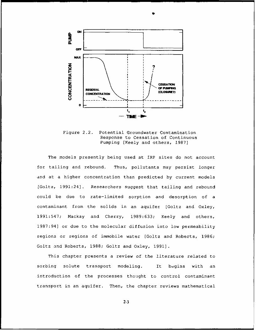
of all residual contaminants (Figure 2.2) [Keely and others,
1987:91; Mackay and Cherry, 1989:633; Travis and Doty,
1990:1465].
2-2
ON
l 1TIMAX
0 I
I CESAT
O OF KPUMINGZ CONCENTRATOO)
ooa
0I-ti t2
T1IME -IP-
Figure 2.2. Potential Groundwater ContaminationResponse to Cessation of ContinuousPumping [Keely and others, 19871
The models presently being used at IRP sites do not account
for tailing and rebound. Thus, pollutants may persist longer
dnd at a higher concentration than predicted by current models
[Goltz, 1991:241. Researchers suggest that tailing and rebound
could be due to rate-limited sorption and desorption of a
contaminant from the solids in an aquifer [Goltz and Oxley,
1991:547; Mackay and Cherry, 1989:633; Keely and others,
1987:94) or due to the molecular diffusion into low permeability
regions or regions of immobile water [Goltz and Roberts, 1986;
Goltz and Roberts, 1988; Goltz and Oxley, 1991].
This chapter presents a review of the literature related to
sorbing solute transport modeling. It begins with an
introduction of the processes thought to control contaminant
transport in an aquifer. Then, the chapter reviews mathematical
2-3

models that account for the sorption process. More
specifically, a model review is presented with a discussion
focusing on the impact and significance of equilibrium
sorption/desorption and rate-limited (nonequilibrium)
sorption/desorption in immobile regions of an aquifer. Next,
the chapter explores the modeling efforts involving pulsed
pumping. Finally, some conclusions are drawn based on the
literature review.
ContamJnant Tranot Processes
To understand contaminant transport modeling, it is first
necessary to describe the various processes thought to control
the subsurface movement of contaminants. For purposes of this
thesis, subsurface refers to the saturated zone (below the water
table) in an aquifer. These processes are related to the flow
of contaminants dissolved in groundwater [National Research
Council, 1990:281. Dissolved contaminant transport is due to a
variety of processes. The National Research Council (NRC)
divides these processes into two groups: (1) mass transport and
(2) mass transfer [National Research Council, 1990: 37].
Mass Transport. Mass transport are physical processes
responsible for fluxes (flow) in the groundwater system. These
mass fluxes occur due to advection, diffusion, and hydrodynamic
dispersion.
Advection is the primary process responsible for contaminant
transport in the subsurface [National Research Council,
1990:37] . Movement of the contaminant mass occurs due to the
24

movement of the groundwater, and in general, it is assumed that
the dissolved mass is transported in the same direction and with
the same velocity as the groundwater [National Research Council,
1990:37; Freeze and Cherry, 1979:389].
Diffusion is the process where contaminant mass spreads due
to molecular constituents moving in response to a concentration
gradient (movement from an area of high concentration to an area
of lower concentration) [Freeze and Cherry, 1979:103]. The
process of diffusion is often referred to as molecular diffusion
or ionic diffusion. Diffusion occurs in the absence of any
movement of solution. If the solution is flowing, diffusion is
partially responsible for contaminant mass mixing [Freeze and
Cherry, 1979:103]. The process of diffusion ceases only when
the concentration gradients become nonexistent.
Hydrodynamic dispersion is a process that accounts for the
spreading of a solute from a path that it would be expected to
follow according to the advective process in a flow system
[Freeze and Cherry, 1979:75] . Because of this spreading,
dispersion causes dilution of the solute; hence, it is a mixing
process. Dispersion can be considered to consist of two
components: mechanical dispersion (mechanical mixing during
fluid advection) and molecular diffusion of the solute particle
[Freeze and Cherry, 1979:75]. Mechanical dispersion occurs as a
consequence of local variability in velocity [National Research
Council, 1990:41]. On a microscopic scale, this variability may
be caused by velocity variations within individual pores or due
2-5

to the branching of pore channels [Freeze and Cherry, 1979:75-
76; National Research Council, 1990:40-41]. The relationship
between mechanical dispersion and molecular diffusion is
dependent upon groundwater flow velocities. At modest flows,
the common assumption is that the molecular diffusion component
of hydrodynamic dispersion is negligible and the mechanical
component is responsible for the spreading. At very slow
groundwater flow velocities, diffusion may dominate
[Environmental Protection Agency 540/4-89/005, 1989:4].
Mass Transfer. Mass transfer processes redistribute
contaminant mass within or between phases through chemical and
biological reactions (National Research Council, 1990:8]. There
is a multitude of these processes, each of them impacting the
transport of a contaminant differently. Of the various
processes, sorption is considered to be one of the most
important since it can have profound effects on contaminant
transport, fate, and removal [Brusseau and Rao, 1989:33; Goltz
and Oxley, 1991:547; Environmental Protection Agency 540/S-
92/016, 1993] T n this thesis, sorption is the only mass
transfer process considered.
The Environmental Protection Agency (EPA) defines sorption
as
the interaction of a contaminant with a solid. Morespecifically, the term can be further divided intoadsorption and absorption. The former refers to anexcess contaminant concentration at the surface of asolid while the latter implies a more or less uniformpenetration of the solid by a contaminant. In mostenvironmental settings, this distinction serves little
2-6

purpose as there is seldom information concerning thespecific nature of the interaction. The term sorptionis used in a generic way to encompass both phenomena.[Environmental Protection Agency 540/S-92/016]
The effect of sorption is to retard or slow the movement of
contaminants in the groundwater. When sorption occurs, the rate
at which the contaminant is transported is lower than would be
the case for an unretarded solute. This process not only
reduces the movement of contaminants in the groundwater, it also
makes it more difficult to remove contaminants from an aquifer.
That is,
the slow desorption of contaminants from the solid tothe liquid phase can significantly reduce theeffectiveness of a pump-and-treat system byprogressively lowering contaminant concentrations inwater pumped to the surface. It is not uncommon topump a system until contaminant concentrations in thepumped water meet a mandated restoration level, whilethe aquifer's solid phase still contains a substantialcontaminant mass. [Environmental Protection Agency540/S-92/016, 1993]
As a result, both the time and cost to remediate to a cleanup
level are increased [National Research Council, 1990:45-46;
Goltz and Oxley, 1991:547; Mackay and Cherry, 1989:633]. The
behavior, transport, and fate of contaminants in the subsurface
is dependent upon the mass transport and mass transfer
reactions, which in turn, depend on contaminant and aquifer
properties [Weber and others, 1991:499].
Advoetion-DiLaprsion-Sorptioin Modala
Mathematical models are commonly used in groundwater studies
to represent those physical and chemical processes that are
2-7

occurring in an aquifer [Goltz, 1991:24; National Research
Council, 1990:1,28,38; Freeze and Cherry, 1979:18-19]. These
models attempt to simulate the actual behavior of contaminant
resulting from these processes by solving mathematical equations
[National Research Council, 1990:52]. These models provide a
source of information about contaminant transport processes that
can assist in the design of remedial programs, risk assessment,
and predict cost and cleanup duration at contaminated sites
[Goltz, 1991:24].
The following sections examine the efforts of researchers to
develop mathematical models to account for the chemical and
physical processes that control sorbing solute transport. The
mathematical formulation of the sorption processes assumes
linear equilibrium, rate-limitation modeled by a two-region
first-order rate process, and rate-limitation due to Fickian
diffusion of the contaminant through immobile water of
cylindrical, spherical, and rectangular geometry.
The mathematical formulation of the physical and chemical
processes that govern dissolved sorbing transport of a single
contaminant in saturated, homogeneous porous media has
traditionally been modeled with advection, dispersion, and a
sink term to describe the transfer of contaminant from the
aqueous phase to the solid phase [Freeze and Cherry, 1979:402].
Equation (2.1) shows, in cylindrical coordinates, the mass
balance equation typically used to account for these processes:
2-8

WC(r, t) D(r) 2C(r, t) V(r) WC(r, t) p aS(r, t) (2.1)-D )0 C
where C(r, t) is the contaminant aqueous concentration [M / 12],
r is the radial coordinate [L], t is time [T], D(r) is the
mobile region hydrodynamic dispersion coefficient [L! I T], V(r)
is the mobile region seepage velocity [L / T], p is the bulk
density of aquifer material [M / V], 0 is the aquifer porosity
[unitless], and S(r, t) is the sorbed contaminant tunitless].
The first, second, and third terms on the right-hand side (rhs)
of the Equation (2.1) represent dispersion, advection, and
sorption of the contaminant, respectively. This equation is the
governing equation for sorbing contaminant transport.
Chen and Woodside presented a mathematical model for the
"basic case" of aquifer decontamination by pumping. That is,
they developed analytical solutions for a single extraction well
operating under a constant pumping rate. Their model describes
converging radial transport for various initial distributions of
contaminant. Transport was assumed to be controlled by
advection and dispersion. Thus, this model does not account for
the effects of sorption [Chen and Woodside, 1988; Goltz and
Oxley, 1991:547].
The models currently in existence that describe sorbing
contaminant transport differ primarily on how the sink term is
represented. The two general approaches that are used to model
2-9

this term are by assuming sorption equilibrium and sorption
nonequilibrium [Brusseau and Rao, 1989:34].
SorMtion Eauilibrium. These models relate the amount of
solute sorbed per unit of sorbent to the amount of solute
retained in the aqueous phase [Weber and others, 1991:505].
Three equilibrium models commonly used to describe this
relationship are the linear, Langmuir, and Freundlich models.
The most common and simplest model to use to simulate
sorbing solute transport assumes an equilibrium, reversible, and
linear relationship between contaminant in the sorbed and the
aqueous phase [Goltz and Oxley, 1991:548; Weber and others,
1991:505]. The assumptions in this simple model are known as
the local equilibrium assumptions (LEA). This implies that the
accumulation of solute by the sorbent is directly proportional
to the solution phase concentration. Mathematically, this
assumption is represented by S = Kd C , where Kd is the
distribution coefficient [12 / M] [Weber and others, 1991:505].
This distribution coefficient describes the distribution of
contaminants between aquifer solids and the groundwater. The
value of Kd is dependent upon the characteristics of both the
contaminant and the aquifer material with the hydrophobicity of
the contaminant and the amount of soil organic carbon playing
important roles in determining the magnitude of Kd
[Environmental Protection Agency 540/S-92/016, 1993]. If we
assume only a fraction, 0, of the total aquifer porosity is
mobile, so .= 0 where 0 m represents the mobile region
2-10

porosity, we may define C'(r, t) as the solute concentration in
the mobile region [M / 1], V, as the mobile region seepage
velocity [L / T], and D. as the mobile region dispersion
coefficient [0 / T]. Substituting the expression
S = Kd CQ(r,t) into the sink term of Equation (2.1) produces
aC' (r, t)_ Dn a2C,(r,t) V. (r) aC' r, t)
SR. a2 Rm Jr
where Rm is the mobile region retardation factor [unitless]
where Rm = I + (p Kd) / 0m This LEA model (linear,
equilibrium) has been found to describe sorption accurately
under certain conditions, most appropriately at very low solute
concentrations and for solids of low sorption potential and low
flow [Weber and others, 1991:505]. According to Brusseau and
Rao,
In order for the LEA to be valid, the rate of thesorption process must be fast relative to the otherprocesses affecting solute concentration (e.g.,advection, hydrodynamic dispersion) so thatequilibrium may be established between the sorbentand the pore fluid. Initially, it was thought that,because of the generally slow movement of water inthe subsurface, equilibrium conditions should prevailand, therefore, the LEA would be valid. Detailedlaboratory and field investigations, however, haverevealed that, in many cases, this assumption isinvalid. [Brusseau and Rao, 1989:41]
When the LEA is justified, the mathematics of sorbing
contaminant transport is greatly simplified [Weber and others,
1991:505].
2-11
The Langmuir model, a nonlinear model, was originally
developed for the case where sorption leads to the deposition of
a single layer of solute molecules on the surface of a sorbent.
The assumptions governing this model are: (1) the energy of
sorption for each molecule is the same and independent of
surface coverage, and (2) sorption occurs only on localized
sites and involves no interactions between sorbed molecules
[Weber and others, 1991:505].
The most widely used nonlinear sorption equilibrium model is
the Freundlich model [Weber and others, 1991:506]. This model
has been applied to simulate sorption on heterogeneous surfaces.
Weber and others indicate that the Langmuir and Freundlich
models are equivalent when describing nonlinear sorption over
moderate ranges of solution concentrations; however, major
differences exist between the models over wide ranges and high
levels of concentration [Weber and others, 1991:506].
Sogrtion Nongamuii•br:ium. It has been proposed that a rate-
limited sorption process is responsible for the concentration
tailing that has been observed in many laboratory and field
observations [Goltz and Oxley, 1991:547; Keely and others,
1987:91; Mackay and Cherry, 1989:630]. In the literature, two
approaches have been used to model these sorption kinetics--
chemical and physical [Brusseau and Rao, 1989:43; Valocchi,
1986:1694]. That is, sorption nonequilibrium is assumed to be
due to either a slow chemical or physical mechanism. In this
section both mechanisms are discussed; however, the primary
2-12

emphasis of this research is on physical sorption
nonequilibrium.
•amUXLL. These models assume that sorption
nonequilibrium results from a rate-limited sorption reaction at
the soil-solution interface [Valocchi, 1986:1694; Brusseau and
Rao, 1989:43]. Valocchi presented a model describing converging
radial transport of a sorbing contaminant. Valocchi's model
assumed a chemical rate-limited sorption reaction described by a
first-order rate law [Valocchi, 1986].
•A. The tailing phenomenon has been
successfully modeled by dividing the porous medium into regions
of mobile and immobile water and modeling advective/dispersive
solute transport in the mobile region (Equation (2.1)) with an
expression to describe the diffusional transfer of contaminant
between the two regions [Goltz and Roberts, 1986:1139; Goltz and
Roberts, 1988:40; Goltz and Oxley, 1991:549]. With these
models, advective/dispersive solute transport is assumed to
occur only in the mobile region and snluf tr;n5---t in the
immobile region is assumed to occur only by diffusion. The
solute transport between the two regions causes the immobile
region to act as a sink or source. Consequently, nonequilibrium
sorption is rate-limited due to the slow transfer of solute
between the two regions [Valocchi, 1986:1694; Brusseau and Rao,
1989:45]. Mathematically, the transport of a single sorbing
solute in a radially flowing aquifer in a porous medium with
2-13

immobile water regions may be written as [Goltz and Oxley,
1991: 548]
aC$* (r, t) D. a 2C'C(r, t) Vm(r) aC$.(r, t) 0 ,R. aC' (r, t)
at Rm 02 R. O 0mRm at
where C' (r,t) is volume-averaged immobile region solute
concentration [M / 12], R. is the immobile region retardation
factor [unitless], 0 m = 0 is the mobile region wdter content
[unitless], and Or = 0 - 0. is the immobile region water
content (unitless]. This expression assumes that sorption onto
the solids is linear and reversible, with the effect of sorption
incorporated into Rm and R,, where Rm = I + (p f Kd) / Om I
Ri = I+ [p(! -f)Kd]J/0n , where f is the fraction of
sorption sites adjacent to regions of mobile water [Goltz and
Roberts, 1988:40].
Various models have been proposed to describe the transfer
of solute between the mobile and immobile regions. The two most
common models found in the literature are first-order rate and
Fickian diffusion [Goltz and Roberts, 1986:1139; Goltz and
Oxley, 1991:548-549; Brusseau and Rao, 1989:46-47].
Firzt-OQdAr Rate. These models assume that solute
transfer between the mobile and immobile regions can be
described by a first-order rate expression [Goltz and Oxley,
1991:5481:
2-14

aC (r, t)- (XR [C'(r, t) - C'(r, t)] (2.4)at 0ir R ý M
where c' [1 / T] is a first-order rate constant The physical
interpretation of Equation (2.4) is based on the assumption that
solute transfer is a function of the solute concentration
difference between the mobile and immobile regions. This model
also assumes that the immobile region is perfectly mixed; thus,
the local concentration at all points within the immobile region
is the same as the volume-averaged immobile region solute
concentration (C ) [Goltz and Oxley, 1991:548]. This
assumption is in contrast to physical diffusion models where a
concentration gradient exists. The combination of Equations
(2.3) and (2.4) are the governing equations describing two-
region first-order sorbing solute transport.
Nkedi-Kizza and others [1984] have shown that the Valocchi's
first-order chemical expression is eciuivalent to physical
nonequilibrium models. In other words, Nkedi-Kizza and others
have suggested that the difference between physical first-order
rate diffusion controlled adsorption and two-site chemical
kinetic adsorption, such as Valocchi's [1986], are
mathematically equivalent when describing ion exchange during
transport through aggregated sorbing media. On a macroscopic
level, both models generate the same total concentration
distribution in the system [Nkedi-Kizza and others, 1984:1129].
2-15

Fiekian Diffupion. The transfer of solute between
the two regions may be assumed to be governed by Fickian (Fick's
second law) diffusion of solute within immobile regions of
specified geometry [Goltz and Oxley, 1991:548-549]. This solute
transfer mechanism requires the presence of a concentration
gradient. As such, the dependent variable in Equation (2.3),
CA, represents a volume-averaged solute concentration within
the immobile region [Goltz and Roberts, 1986:1140]. C'(r,t) is
defined by [Goltz and Oxley, 1991:548]
C (r, t) = aQ z'-' C(r, z, t)dz (2.5)
where C'(r,z,t) is the local concentration at points within the
immobile region [M / 12], = 1,2, 3 for rectangular (layered),
cylindrical, and spherical immobile region geometry,
respectively, a is the immobile region radius or half width [L],
and Z is the coordinate within the immobile region [n].
Mathematically, Fick's second law of diffusion, describing
contaminant transport within the immobile region, is
RdC(r, z, 0 D (2.6)
where D' is the immobile region solute diffusion coefficient
Figure 2.3 shows an idealized conceptualization of an
aquifer remediation by pumping where the transfer of solute
2-16

between mobile and immobile regions may be affected by first-
order rate or Fickian diffusion rate-limiting mechanisms [Goltz
and Oxley, 1991:549].
kV~ally caritainad mare
- -//.- A//
'//
SIm m -a bl -r , € o m ., l .'
-NU7
•FI-are ra,. -. 1.-- r
Figure 2.3. Conceptualization of Aquifer Remediation, WhereContaminant Transfer May Be Affected by Rate-Limiting Mechanisms [Goltz and Oxley, 19911
In summary, the differential equations that govern dissolved
sorbing solute transport consist of Equation (2.3) (with the
last term not present) for the local equilibrium assumption,
Equations (2.3) and (2.4) for the two-region first-order rate
2-17

assumption, and Equations (2.3), (2.5), and (2.6) for the
diffusion assumptions.
Pulsmd UPMumin
As previously mentioned, pump and treat is the most commonly
used technology for remediating contaminated aquifers.
"Approximately 68% of Superfund Records of Decision (RODs)
select pumping and treating as the final remedy to achieve
aquifer remediation" [Travis and Doty, 1990:1465]. In fact, pump
and treat technology is the preferred method to restore
contaminated aquifers to drinking water quality [Olsen and
Kavanau,,i, 1993:42]. The literature reviewed has, for the most
part, criticized pump and treat technology primarily due to its
ineffectiveness in achieving health-based cleanup standards
coupled with extended periods of cleanup duration and high cost.
The most significant literature reviewed was an EPA study
involving 19 sites where pump and treat remediation had been
ongoing for up to 10 years [Environmental Protection Agency
540/2-89/054, 1989]. This study revealed
Of the 19 sites studied in detail, 13 had aquiferrestoration as their primary goal, and only 1 hasbeen successful so far. Several of the other systemsshow promise of eventual aquifer restoration, buttypically progress toward this goal is behindschedule. Concentrations often decline rapidly whenthe extraction system is first turned on, but afterthe initial decrease continued reductions are usuallyslower than expected. [Environmental ProtectionAgency 540/2-89/054, 1989]
2-18

The EPA further indicated that although significant removal of
contaminant mass was achieved, the concentration levels
remaining in the aquifer were generally above health-based
standards or site-specific cleanup objectives. As a result, the
systems had been operating longer than the predicted time
required for cleanup [Environmental Protection Agency 540/2-
89/054, 1989:E-l-E-3, 2-13].
The previous section discussed how rate-limited
sorption/desorption tends to slow the removal of contaminants
from an aquifer as the groundwater is pumped. In turn, pump and
treat remediation is often rendered ineffective. Therefore,
there is great interest in evaluating alternative pumping
schemes that can account for rate-limited sorption/desorption.
One proposed approach is pulsed pumping. Under a pulsed pumping
scheme, pumps are shut off for periods of time so that slow
desorption would occur. When the pumps are turned on again,
higher concentrations would be removed [Goltz, 1991:25; Keely
and others, 1987; Borden and Kao, 1992:34; Mackay and Cherry,
1989:633; Haley and others, 1991:124; Environmental Protection
Agency 540/2-89/054, 1989]. It has been suggested that this
cycling of extraction wells on and off in 'active' and 'resting'
phases may remove the minimum volume of contaminated
groundwater, at the maximum possible concentration, for the most
efficient treatment (Figure 2.4) [Keely and others, 1987:94-99].
2-19

MAX"
---------------------------------- I----I ='-- -•
41 t2 13 14 25 to or
- TIME -'-
Figure 2.4. Potential Effluent Concentrations for PulsedPumping Remediation [Keely and others, 1987]
The literature reviewed has identified sources that
qualitatively discuss pulsed pumping as a pump and treat
enhancer; however, the only mathematical analysis incorporating
pulsed pumping with the advection/dispersion equation is an
unpublished document by Carlson and others [Carlson and others,
19931.
Carlson and others mathematically derived the solutions in
the Laplace domain for contaminant concentration for the cases
of linear equilibrium, two-region first-order rate, and Fickian
diffusion. Carlson and others research extends the work of
Goltz and Oxley [1991] in that their derivation takes into
account conditions when the pump is on and when the pump is off,
whereas Goltz and Oxley's solutions required the pump to be
continuously on. Unfortunately, Carlson and others did not
2-20

numerically evaluate the Laplace domain solution nor convert it
back to the time domain.
Groundwater extraction or pump and treat is the most
commonly used remediation technology for aquifer
decontamination. However, it has been criticized for its
inability to attain health-based cleanup standards, meet
projected timelines, and stay within budget. The literature
indicates that part of the limitations of pump and treat are due
to the various processes occurring in an aquifer. Understanding
the physical and chemical processes which dictate the transport,
fate, and removal of contaminants in groundwater is essential in
designing and implementing more effective and efficient
remediation systems at IRP hazardous waste sites. Mathematical
models have proven to be excellent tools for representing the
effects of the various processes--advection, dispersion,
sorption, and diffusion--that can occur simultaneously in an
aquifer and affect the transport and concentration of
pollutants.
The literature search revealed three commonly used sorbing
solute transport models: linear equilibrium, two-region first-
order rate, and Fickian diffusion. The significant difference
among these models is the underlying assumptions used in their
development. The linear equilibrium model assumes an
instantaneous equilibrium between the aqueous and sorbed
contaminant phases, whereas the two-region first-order rate and
2-21

the Fickian diffusion models are based on the premise that a
nonequilibrium condition exists, and solute transport is rate-
limited due to the transfer of the contaminant between regions
of mobile and immobile water. The appropriateness of any one of
these models is dependent upon actual site conditions. In fact,
rate-limited sorption/desorption has been studied by several
researchers who propose that this phenomenon is responsible for
the 'tailing' and 'rebound' that have been observed in numerous
field and laboratory studies and one 'culprit' responsible for
the ineffectiveness of pump and treat systems. As a result,
pump and treat enhancers which account for this behavior, such
as pulsed pumpin-> are being investigated.
The literature reviewed has shown that the only significant
attempt to model a pulsed pumping scheme under conditions of
rate-limited sorption/desorption was the research proposed by
Carlson and others. The literature clearly shows a need for
continued research in this area. Further efforts are needed to
numerically evaluate their solutions.
This thesis will extend Carlson and others work by
developing a source code based on their solutions. It is
intended that this research may provide IRP decision makers with
a better understanding of the physics that can occur in an
aquifer, and help them validate more complex numerical models
that are used to predict the level of cleanup required, duration
of cleanup efforts, and the cost associated with aquifer
remediation.
2-22

The primary objective of this research is to develop a
computer model describing contaminant transport by means of
radial advection, dispersion, and sorption in an aquifer
undergoing pulsed pumping operations. Since this research
extends the work of Goltz and Oxley [1991] and Carlson and
others [1993], the equations, solutions, notation, and source
code will be based on the expressions of sorption presented in
their respective papers.
In order to establish the basis of the equation set, model
assumptions and aquifer characteristics are reviewed. Then, the
governing equations and their solutions, which are used to
develop the source code, are presented.
M•dl Asamtiona and Aquifer Cha-antritica
As stated in Chapter I, in order to model contaminant
transport analytically, model equations must be simple. The
simplifying assumptions used in this research represent an
'idealized' scenario.
One key assumption used to set up the model was the
assumption that contaminant transport is described by steady,
uniform, converging radial flow resulting from advection due to
the extraction well. Thus, transport due to the natural
groundwater gradient is assumed negligible. Coupled with this
3-1

assumption, the drawdown of the aquifer water table due 4-o the
pumping is also considered negligible.
To take advantage of radial symmetry, we assumed that a
single, fully penetrating extraction well is in operation placed
at the center of a cylindrically symmetrical contaminated
region. In addition, the initial contamination distribution was
also assumed to be radially symmetric.
Another significant assumption used to set up the model is a
single, infinite, homogeneous, and unconfined aquifer.
Furthermore, the aquifer was considered to be of constant
thickness and bounded by a horizontal aquitard with no seepage.
In addition to the assumptions listed above, model
development was based on the concept of physical sorption
nonequilibrium as discussed in Chapter II. Therefore, to
understand the formulation of the model, it is necessary to
review this concept. Recall that in Chapter II, we discussed
how solute transfer can be modeled by dividing the porous medium
into regions of mobile and immobile water. Advective and
dispersive solute transport occurs in the mobile region, and an
additional term is used to describe the diffusional transfer of
contaminant between the two regions [Goltz and Roberts,
1986:1139; Goltz and Roberts, 1988:40; Goltz and Oxley,
1991:549]. The transfer of solute between mobile and immobile
water may be assumed to be governed by either Fickian diffusion
of solute within immobile regions of layered, cylindrical, and
spherical geometry or by a first-order rate expression [Goltz
3-2

and Oxley, 1991:548-5491. Goltz and Oxley presented a
conceptual i zat ion of mobile and immobile water regions in an
aquifer where contaminant transfer may be affected by Fickian
diffusion or a first-order rate process (Figure 2.3).
If we combine the simplifying assumptions and the concept of
physical nonequilibrium, we can now describe the aquifer
characteristics associated with formulating the model.
Consider an extraction well of radius r,, [L] pumping at a
rate Q. [ 12 / Tj placed at the center of a cylindrically
symmetric contaminated region of radius r. (L] in an aquifer of
constant thickness b (L]. In this contaminated region assume
there exists mobile and immobile water regions. General
properties associated within the mobile region consists of the
mobile region water content, 0. (dimensionless], mobile
retardation factor, R. [dimensionless], and longitudinal
dispersivity, a, [L]. Immobile water region properties consists
of the immobile region water content, 0im [dimensionless],
immobile retardation factor, Rim (dimensionless], and the
immobile region solute diffusion coefficient, D'C [12 / T]. If
the transfer of solute between the two regions is assumed to be
governed by Fickian diffusion, then another property associated
with the immobile region is the radius of the spherical or
cylindrical regions or half width of the layered region, a (L].
Initially in the contaminated region there exists some
maximum concentration in the mobile and immobile regions, C.'
[M / 12]. If we define the initial solute concentration
3-3

distribution in the mobile region as F,(r) [M / 12], and the
volume-averaged initial solute concentration in the immobile
region as Fi(r) [M / 12], then at a later time, t (T], we now
define the mobile region solute concentration as CQ(r, t)
[M I 1] and the volume-averaged immobile region solute
concentration as C'(r,t) [M / 12
In the case where the immobile region is geometry dependent
(Fickian diffusion), initially there exists some local solute
concentration at points within this region, F.(r, z) [M / V].
This concentration is not only a function of the radial
distance, r [L], but also its radial position within the
immobile region, Z [h]. As time progresses, we define the local
solute concentration at points within the immobile region as
Ca(r,z,t) [M / 12].
Governing Equations and Solutions
Chapter II introduced the theoretical development of the
differential equations for sorbing solute transport. This
section presents the governing equations and solutions for
sorbing solute transport for conditions when an extraction well
is on and when an extraction well is off. The model equations
allow for arbitrary initial conditions and are developed for the
following sorption assumptions: linear equilibrium, rate-limited
modeled by a two-region first-order rate process, and rate-
limited due to Fickian diffusion of the contaminant through
immobile water regions of layered, cylindrical, and spherical
3-4

geometry. A more detailed mathematical analysis can be found at
Appendix A and a list of the variables or notation used in this
thesis on page viii.
Mndel rorlation: Xxt~raoion Well O. As presented in
Chapter II, the expression governing contaminant transport
within the mobile region of a homogenous, radially flowing
aquifer is
WC'(r,t) D. a2C' (r,t) 0 V (r) aC' (r, t) O, R,= WC (r, t) (3.1)
it Rm (2 Rm Or 0zRm ct
for r. < r < r. and t > 0 and C'(r,t) is defined by [Goltz and
Oxley, 1991:548]
Ci(r, t) = a z'-'C (r, z, t)dz (3.2)
for r, < r < r. and t >0 and 0< z < a. Given an aquifer of
constant thickness, b [L], and an extraction well pumping at a
rate Q, [L / T], then the radial velocity is
Vm(r) = Q. (3.3)2 ntbOmr
Assuming that the mobile region dispersion coefficient, Dm
[L2 I T], is given by
D.(r) = a, IVm(r)I (3.4)
3-5

and that the mobile region molecular diffusion coefficient,
D' << D., and defining the dimensionless variables as
r (3.5)al
2T -bORa 2 (3.6)
C'0
Ci= X, T -C' (r, t)C,(X T) inc" (3.8)0
and the dimensionless constant
Oi 0 RIM (3.9)8.ROmRm
where X is the dimensionless radial distance, T is the
dimensionless time, Cm(X,T) is the dimensionless mobile region
solute concentration, C• (X,T) is the dimensionless volume-
averaged immobile region solute concentration, then Equation
(3.1) can be rewritten in dimensionless form as
aCm (X, T) _ I 2 Cm (X, T) I Cm (X, T) aC. (X, T)x+ x x(3.)
3-6

for X. < X < X. where X, is the nondimensionalized well radius
and X, = r, / a,, and X. is the nondimensionalized contaminated
area radius and X. = r. / a, for T > 0.
The use of the mobile retardation factor, R., and immobile
retardation factor, R., is based on the assumption that there
is an instantaneous equilibration between the aqueous and sorbed
contaminant within the mobile and immobile regions, whereas the
sorption rate limitation is due to the slow diffusive release of
solute between the two regions [Goltz and Oxley, 1991:548].
The third term on the right-hand side of Equations (3.1) and
(3.10) represents the accumulation of the contaminant within
immobile regions (Goltz and Oxley, 1991:548]. As previously
discussed, this term can be modeled assuming that immobile
regions do not exist (local equilibrium), or that two region
transfer of solute can be described by a first-order rate
expression, or that Fickian diffusion governs the transfer of
solute within immobile regions of layerea, cylindrical, and
spherical geometry [Goltz and Oxley, 1991:548-549].
The simplest model used assumes that contaminant transport
is through the mobile region only. Sorption is instantaneous.
This model, commonly referred to as the local equilibrium
assumption, assumes P = 0 which implies all the water is
mobile and therefore it does not account for immobile water
regions [Goltz and Oxley, 1991:548].
3-7

Another assumption often made is that the transfer of solute
between the mobile and immobile region can be described using a
first-order rate expression:
aC' (r, t) a'~C~ t)- a [C'(r, t) - C'(r, t)] (3.11)at OiiRimi
where X is a first-order rate constant [TV]. Defining a
dimensionless first-order rate constant a as
a 2i•bal 2
a = (3.12)
and using Equations (3.5) through (3.8) gives the expression
aC (XT) = a[Cm(X,T) - C (X,T)] (3.13)
aT
This model assumes that the immobile region is perfectly mixed;
thus, the local concentration at all points within the immob'ile
region is the same as the volume-averaged immobile region solute
concentration [Goltz and Oxley, 1991:548].
Finally, it is often assumed that the transfer of solute
between the mobile and immobile regions is governed by Fickian
(Fick's second law) diffusion within immobile regions of
specified geometry [Goltz and Oxley, 1991:548-549].
Mathematically, Fick's second law of clffusion describing
contaminant transport within the immobile region is
3-8
Rm (r,z,t) - D a C' (r, z, t) (3.14)at z•-' U z- az.
where 0 < z < a. When U = 1 diffusion is assumed to occur
through a rectangular or layered immobile region; when ) = 2,
diffusion is assumed to occur through a cylindrical immobile
region; and when v = 3 diffusion is assumed to occur through
a spherical immobile region [Goltz and Oxley, 1991:549; Goltz
and Roberts, 1987]. Defining a dimensionless immobile region
solute diffusion coefficient, D., as
D'a 2 2 bdO R.D,= e 1 miR(3.15)
a 2Q wRi
and the dimensionless immobile region variable, Z, and
dimensionless local solute concentration at points within the
immobile region, C,(X,Z,T), as
zZ -(3.16)
a
C.(XZ,T) = C'(r,z,t) (3.17)C'a
changes Equation (3.14) to
aCa(X,Z,T) _ D, (X, ZxT)1 (3.18)a)T Z U-I aZ aZ(31)
for 0 < Z < 1 and Equation (3.8) to
3-9

C (X,T) = Z-' C. (X, Z, T) dZ (3.19)
Having described the aquifer characteristics, model
assumptions, and dimensionless variables, the following initial
and boundary conditions can be formulated for the various
models.
Initial eonditio, . The initial conditions are
C.(X, T = 0) Fm(X) X. < X < X. (3.20)
C (X,T = 0) F (X) X. < X < X. (3.21)
Cm(XT = 0) = Ci(X,T = 0) = 0 X > X. (3.22)
where Fm (X) and Fm (X) are dimensionless arbitrary initial
concentration conditions in the mobile region and immobile
region, respectively. The diffusion models require the
following additional initial conditions tc describe transport
within the immobile regions [Goltz and Oxley, 1991:549-550]:
C,(XZ,T = 0) = F.(XZ) X, < X < X. (3.23)
C.(X,Z,T = 0) = 0 X > X. (3.24)
where F. (X, Z) is the dimensionless arbitrary initial
concentration condition in the immobile region of a certain
geometry. Again, Equations (3.20), (3.21), (3.22), (3.23), and
(3.24) state the initial conditions, which assume contamination
3-10

of mobile and immobile regions at some arbitrary concentration
within a cylindrical region of dimensionless radius X..
BoundarW ConditionL . The outer boundary condition is
derived based on the assumption that the total mass flux irward
at the outer boundary (X = X.) must always be zero, since
initially, there is no contaminant mass at X > X.. That is,
C'(r., t) + ( t) = 0 (3.25)
using Equations (3.5) and (3.6) changes this expressior .nto
dimensionless form:
Cm(X., T) + --- (X., T) = 0 (3.26)ax
The boundary condition at the well radius is based on the
assumption that at any time, the concentration inside the well
bore is equal to that entering the well from surrounding media
[Goltz and Oxley, 1991:549]. This implies a zero concentration
gradient at the interface between the well and its immediate
adjacent aquifer. Thus,
ac' (r"' t) = 0 (3.27)
Again, using Equations (3.5) and (3.6) changes this expression
into dimensionless form:
3-11

(X.,T) = 0 (3.28)
The diffusion models require additional boundary conditions to
describe transport within the immobile regions of certain
geometry. We assume that the concentration gradient within an
immobile region of certain geometry is zero at the center due to
radial symmetry and is equal to the mobile region concentration
at its outer boundary. Therefore,
ac'-Z (r, z = 0, t) = 0 r < r (3.29)
C'(r,z = 1,t) = C'(r,t) 0 r < r (3.30)
or in dimensionless form, using Equation (3.17), gives us
c (X, Z = 0, T) = 0 X" < X (3.31)
C,(X,Z = 1,T) = Cm(XT) X. < X (3.32)
Laplace TransAorm. In this section we introduce a
mathematical technique that is often used in the solution of
boundary-value problems. This technique is known as the Laplace
transform, which converts a boundary-value problem involving a
linear differential equation as a function of time into an
algebraic problem involving the Laplace transform variable S
[Ross, 1980:427]. Ross defines the Laplace transform by
F(s) = e" e f(t)dt (3.33)
3-12

for all values of S for which the integral exists, where f is a
real-valued function of the real variable t, defined for t > 0
and S is a variable that is assumed to be real [Ross, 1980:427).
The function F defined by the integral is called the Laplace
transform of the function f. The Laplace transform F of f is
denoted by L{f} and F(s) by Z{f(t)J [Ross, 1980:427].
One of the basic properties of the Laplace transform used in
developing the model equations is the Laplace transform of the
derivative of f. That is, if f is a real function that is
continuous for t Ž 0 and of exponential order ec', and f', the
derivative of f, is piecewise continuous in every finite closed
interval 0 • t ! b then Z{f'(t)} exists for S > Cc [Ross,
1980:435]. Thus,
S= s L{f(t)} - f(0) (3.34)
La4lace Solution. In this section we present the
general Laplace solution for when an extraction well is on.
Details of the derivation can be found at Appendix A.
Taking the Laplace transform of Equation (3.10) together
with the appropriate conditions for the various models, yields
- + X y X Cm = F(X, s) (3.35)
where the overbar indicates the transformed function and y and
F(X, s) are given for the various models as follows.
3-13

Local Equilibrium Model (LEA):
Y= S (3.36)
F(X,s) = -XF.(X) (3.37)
First-Order Rate Model:
y= sI + +•a) (3.38)
F(X, s) = -X(F (X) + PF• (X) (3.39)
Layered Diffusion:
) COsinh o (3.40)
F(X, s) = X[Fm (X) + p J'cosh(,A) F. (X, 4)d4 (3.41)
where 0O = (s / De)1/2
Cylindrical Diffusion:
ly = S+ 2 I (3.42)
F(X, s) = -X[Fm(X) + 2p JIo(O)Fa(Xi )d4] (3.43)3 o1 0 4 )
3-14

where (0 = (s / D.)'/ 2 , and 10 and I, denote the modified Bessel
functions of the first kind of order zero and one, respectively.
Spherical Diffusion:
-- -+ 30 1 (3.44)L 0io ((0
F(X, s) = XF,, (X) + i3(--(X,- (3.45)1o (0)) 0 4 o F
where w = (s / D.)" 2 , and i0 and i1 denote the modified
spherical Bessel functions of the first kind of order zero and
one, respectively.
Green'n I'unetion. Now assume that Equation (3.35)
has a solution of the form
-- XI
Cm(X,S) = *(X,s)e 2 (3.46)
Substituting Equation (3.46) into Equation (3.35) yields
- y, + 4 F(X, s) (3.47)
3-15

and upon letting y = y3[X + (1 / 4y)] and
4 (y, s) = M(X, s) = 0 (y- y - I / (4y), s ,Equation (3.35)
becomes
d 2 ,-2/3 -[ 1 S
•=i , -exp [ y y , y Y 4(y,S)dy 24 4
(3.48)
for y, < y < y. where (D is now a function of y and s. If we
also substitute Equation (3.46), and use the above definitions
for y = y. , y = y. , into Equations (3.26) and (3.28) we
get the boundary conditions
l1, dOb-D(y,) + y3 _ (y .,) = 0 (3.49)
2 dy
I d4D y.) = 0 (3.50)2 dy
It is well known that Equation (3.48) has a solution of the
form [Ritger and Rose, 1968]
4)(y, s) = J" g(y, T1, s) .(TI, s) dTl (3.51)
where g(y, ,s) is the Green's function given by
3-16

•(Y) (D)2 (TO)
w[J , 0210() Y < 11 - Y.g(Y, n, s) = (3.52)14), (r) c1
2 (y)WI[4T,4D2 ](I() Y, < T)I - Y
where 0I1 satisfies Equations (3.48) and (3.49), 02 satisfies
Equations (3.48) and (3.50), W[ 1),4) 2](I1) is the Wronskian of
41 and 02 If we define the following operators, G and H, as
G[Ai](y ) = -] Ai (y,,) + 7'd i( .)( .3
2 dy
3 dAiG[Ai](y,) = -- i(y- -y (+,Y ) (3.55)
2 dy
H[Ai](y,) I = Bi(y,,) + 'y-y, 3.5
SdBiH[Bi](y.) = -Bi(y) (y.+ (3.56)
2 dy
where Ai and Bi are Airy and Bairy functions, respectively,
then,
4 1,(y) = G[Bi](y.,)Ai(y) - G[Ai](y,,)Bi(y) (3.57)
0 2 (y) = H[Bi](y.)Ai(y) - H[Ai](y.)Bi(y) (3.58)
3-17
and the value of the Wronskian is
2 G(Ai](y,) H[Ai](y.)i 1 (3.59)W(, 2 ](Y) ]y.) H[Bi](y.) x
Substituting Equations (3.57), (3.58), and (3.59) into Equation
(3.52) yields
x[G[Bi](y.)Ai(y) - G[Ai](y.)Bi(y)][H[Bi](y. )Ai(-q) - H[Ai)(y. )Bi(,)]G(Ai](y, )H[Bi](y.) - G[BiJ(y, )H[Ai](y.)
g(y, 11) =
1 _I G[Bi](y.)Ai(1T) - G[Ai](y.)Bi(TI)][H[Bi](y.)Ai(y) - H[Ai](y.)Bi(y)]
G[Ai](y,)H[Bi](y.) - G[Bi](y.)H[Ai](y.)
(3.60)
where the top expression is defined for the interval y < 11 _< y.
and the bottom expression is defined for the intervalI
Y, 5 11 < y. Since y = 9y[X + (1I 4y)] then
T1 = Y +3 dl = y' d4 (3.61)
[ 4j ly
Thus, Equation (3.51) becomes
ix. 1 [ 1 + +/ 1 Y dýV(X) = g + -y + s4y3%+ 4y s4y
(3.62)
3-18

or alternatively, using C.(X,s) =(X,s)e 2 from Equation
(3.46j
C (X, s) = e gY[X + 4 3 + (, S) d
(3.63)
If we define
b(X, ,s) = g (Y3x + 4-], 'Y3 + + , s (3.64)
then1 I~
Cm(X, s) = exJ b(X, , s) ' 3 e 2 ' F(, s)dý (3.65)
Substituting in the constructed Green's function from Equation
(3.60) gives us
3-19

Cm(, s = G[Ai](y.)H(Bi](y.) G(Bi](y.)H[Ai](y.)}
-G[Bi](y.)H[Ai](y. )Bi[Ty +4 ~fjx~i Y e(2+ (4, S)d4
+GAi(y H[iJy.)I[Y(X + )LK]Jxx~i[yl( + ]etf(4, s)dý
-G[Ai](y.,)H[Bi](y.)Bi[Y3( +y 4y]f4~(
+G[Ai](y,.)H[Ai](y.)Bi y3(x + +ji B~i[,yl(4 +I eitf(,sd
-G[Bi](y,,)H[Ai](y.)Ai y3 x + Ixj B[,y3 + e' , s)d4}
4(3.66
+G[Bi](y,)H[Bi](y.Ai y x +-'2]x0 i-,ý+sd

Modal Fomilation: Erztract-ion Wll Off. If we now consider
turning off the extraction well (Qw = 0) after a certain period
of time, say T, then the mobile region dispersion coefficient,
Dm = 0 (Equation (3.1)), and the molecular diffusion
coefficient, D', becomes the dominant transport mechanism. As a
result, Equation (3.1) becomes
WC'(r,t) - D' I D r _C' (r,t)_ W' _(r,_ t)t r r r)irCnt (3.67)
If we define the dimensionless variables
r D:gRma D" RX (3.68)a R
T = R 2 (3.69)
then Equation (3.67) becomes
WC (X, T) _ 2C, (X X, ICm(X, T) W., (X,T)+ (3.70)
)T aX 2 aX X aT
Notice that this X and T are different from those defined in
Equations (3.5) and (3.6). Similarly, if we define
zz = - (3.71)
a
3-21

which is the same as previously defined in Equation (3.16), then
Equation (3.14) becomes
W. a(X, ZT) _ 1 ZU- W. (X, Z,T)1 0 < Z < 1(3.72)O-Yr z U' azL az JI
To attain a form of the solution when the extraction well is
off, we will assume that the arbitrary initial conditions are of
the same form as the initial conditions when the well is on,
except for two significant differences. First, the initial
conditions are at some later time, T = T , rather than at
time T = 0 This time (T) reflects the contaminant
concentration in the mobile and immobile regions at the time the
extraction well is turned off. Thus, the initial conditions at
T are the terminal conditions for the pump on. Second, the
dimensionless variables, X, X,, X,, and T take on a different
meaning and form from the pump on case. From Equation (3.68) we
have
Xwrw D: Rr.W = ~ (3.73)a R
X.=r R (3.74)a D' R
Thus, the form of Equations (3.20), (3.21), (3.22), (3.23), and
(3.24) are applicable as the initial conditions for when an
extraction well is off.
3-22

The boundary condition at the well for the pump on case is
still assumed to be applicable when the pump is off (Equation
(3.28)). That is, we assume that the concentration inside the
well bore is equal to that entering the well from the
surrounding media. Similarly, the boundary conditions within
the immobile regions of layered, cylindrical, and spherical
geometry remain as stated in Equations (3.31) and (3.32).
The outer boundary condition is modified to allow for
leakage of the contaminant, since molecular diffusion is assumed
to be the dominant mechanism responsible for transport. Thus,
we assume that the total mass flux outward at the outer boundary
of the contamination region (r.) is proportional to the amount of
the contaminant mass present in the mobile region.
Mathematically, this boundary condition is represented as
Ec (X.,T C. (XoiT (3.75)
where £ represents the coefficient of leakage [dimensionless] of
the contaminant through the outer boundary. Refer to Appendix A
for the derivation of this boundary condition.
Laplace Solution. As previously discussed, using the
Laplace transform, the general Laplace solution for when an
extraction well is off is derived. Details of the derivation
can be found at Appendix A.
Combining the Laplace transform of Equation (3.70) together
with the appropriate conditions for the various models, yields
3-23

a2 + yC = F(X, S)x xa (3.76)
where the overbar indicates the transformed function and y and
F(X, s) are given for the various models as follows.
Local Equilibrium Model (LEA):
y =s (3.77)
F(X,s) = -F.(X) (3.78)
First-Order Rate Model:
S I + (3.79)
F(X, s) = -*Fm(X) + OaFf. (X) (3.80)
Layered Diffusion:
+ = sinh0)cos (3.81)
F(X, s) =[Fm (X) + I0cosh(g) F. (X, ý)d4 (3.82)
where (0 = (S) 1/2
3-24

Cylindrical Diffusion:
F = + Io(w ) (3.83)
"F(X,s) = -[Fm(X) + i 0(o))--A)F.(X,)< (3.84)
where (0 = (s) 11 2 , and 10 and 1 denote the modified Bessel
functions of the first kind of order zero and one, respectively.
Spherical Diffusion:
S= s + 3P it (0) 1 (3.85)3 0 io(0)) 1
F(X,s) = -[F,.(X) + 3- 2 i-o(o)F.(X, 4)d4 (3.86)
where (0 = (S)1 1 2 , and i0 and i1 denote the modified spherical
Bessel functions of the first kind of order zero and one,
respectively.
Green's Funatin. As before, we construct a Green's
function by assuming that Equation (3.76) has a solution of the
form
Cm (X, S) = *(X, S) (3.87)
3-25

such that this solution satisfies the differential equation
(Equation (3.76)) and the boundary conditions (Equations (3.28)
and (3.75)). Substituting Equation (3.87) into Equation (3.76)
yields
d 2 0(X, S) 1 doX, s) _ 0(X, s) = F(X, s) (3.88)
dx2 X dX
and upon letting y = YI/ 2 X , and
O(X,s) = 0(y1-/2 y, s) = D(y,s) , Equation (3.88) becomes
d2cb(y, s) + I dcb(y, s) - 4D(y s = 1 (y's) (3.89)
dy2 y dy
for y, < y < y., where Y(y, S) = (y-1/2y, s) and 4 is now a
function of y and s. If we also substitute Equation (3.87), and
use the above definitions for Y = Y. Y = Y. into
Equations (3.28) and (3.75) we get the boundary conditions
d(y"'s) = 0 (3.90)dy
1 d4C2y (y,,S) - 4(y, S) = 0 (3.91)
It is well known that Equation (3.89) has a solution of the
form [Ritger and Rose, 1968]
D(y, s) = g(y, r1, s) ,(T], s) di (3.92)3y-
3 -26

where g(y, TI,s) is the Green's function given by
, ( b,](TO Y < TI 5 Y.
g(y, TI, s) = (3.93)4D 1 (TO) 4(2 (y)
where 4It satisfies Equation (3.89) and (3.90), 02 satisfies
Equation (3.89) and (3.91) and W[I0, 1 4 2 ](D1) is the Wronskian of
4D, and 02 Thus,
0 ,(y,s) = -Ko(y,,) 0o(y) + I'(y,,) Ko(y) (3.94)
(D 2 (yS) = H[K1 , Ko](y.) I0 (y) + G[11, Io](y,) Ko(y) (3.95)
where K0 and 10 are modified Bessel functions of the third kind
order zero and first kind order zero, respectively, and I, is a
Bessel function of the first kind order one and is equal to 1,
and KI is a Bessel function of the third kind order one and is
equal to -K' [Abramowitz and Stegun, 19701. Also, G and H are
operators defined by
I
G[11, 10 ](y.) = Ey2 1• (y.)- o((y.) (3.96)
H[K1 ,K0](y.) = Cy2 K,(y.) + Ko(y.) (3.97)
3-27

and the value of the Wronskian is
W[4), >,1](y) = -[I,(y.)H[Kj,Ko](y.) - KI(y.)G[l, Io](y.)]Y
(3.96)
Substituting Equations (3.94), (3.95), and (3.98) into Equation
(3.93) yields
T1[K,(y.)I,(y) + I1 (y.)K 0 (y)][H[Kj, Ko](y.)I,(T) + G[I,, I.](y.)K(n1)]
I1 (y.)H[K,, K0 ](y.) - K, (y,)G[I1 , 1.](Y.)g(y, T, s) =
in[K,(y.)Io(q) + I1(y.)K,(q)][H[K,, Ko](y.)Io(y) + G[1 1, I.](y.)Ko(Y)]I1,(y.)H[Kl, Ko](y.) - K,(y.)G[I,. I,(y.)
(3.99)
where the top expression is defined for the interval y _< 11 _< y.
and the bottom expression is defined for the interval
Y, :5 T] < y. Since (D(y) = O(X) then
1 1
TI = 7'4; d1j = Y' d4 (3.100)
Thus, Equation (3.89) becomes
(y' S) = J'g Y2X, Y2 ,S i y2 d4 (3.101)
3-28

Since C,(X, s) = 0(y, s) (Equation (3.87)), then
CU(X,s) = Jg y X, y2 F(4 s)d4 (3.102)
If we define
b(X, 4, s) = g (,Y X, y2 4, s (3.103)
then
Cm (X, S) = 4(x , S) y 2 N({, S) d4 (3.104)
Substituting in the constructed Green's function (Equation
(3.99)) gives us
3-29

Cm(,S){I(y.)H[K1,Ko](y.)- K,(yw.)G[, Ii,, ](y.1
{H[Ki, Ko](Y.)IO(y 2X) + G [1,, 10 ](y.)4K0 (y 2X) K, (Y.) )J ej (y y24) )F (, S d
+ HKIK,,(Y.Io (y2X ~ ,~ K 0 ](y2X)]O Ii[ K ) K0 ](Y. )Jx 1 (2 )f ( 4, s) d4
+KIyWIo~y2X) + Iy)Kyix I[, o(. x (,sd
(3.105)
3-30

5. Ana~lysis and Evaluation of Rasults
This chapter presents results using a computer model based
on the analysis developed in Chapter III. First, a discussion
of the numerical techniques and difficulties encountered in
coding the analytical solutions is presented. Then, model
simulations, showing the transport and fate of a contaminant
undergoing pulsed and continuous pumping, are presented for
varying initial conditions. Finally, model verification is
attempted by comparing model results with two existing models
that incorporate rate-limited sorption and desorption.
Numarinal ZEvaluatinn
Because of the complex nature of the Laplace solutions
presented in Chapter III (Equations (3.66) and (3.105)), the
formula translation (FORTRAN) language was used. Being one of
the older scientific computer languages, the FORTRAN language
has the advantage of accessing large mathematical libraries.
Incorporating sophisticated, well-tested functions and routines
from these libraries, the model is able to numerically solve the
Laplace solutions. Specifically, the model uses the Stehfest
algorithm [Stehfest, 1970], Gauss-Quadrature integration [Press
and others, 1992), and the International Mathematical and
Statistical Library (IMSL) function package SFUN [International
Mathematical and Statistical Library, 1989]. For detailed
4-1

information concerning the model's numerical and logical
architecture, refer to the systems level flowchart at Appendix B
and the FORTRAN source code at Appendix C.
Lalarem Irkneralon. As stated in Chapter III, the primary
objective of this research is to develop a working computer
model describing contaminant transport by means of radial
advection, dispersion, and sorption/desorption in an aquifer
undergoing pulsed pumping operations.
As shown in Chapter III, the solutions used to develop the
code are in the Laplace domain. Therefore, the primary purpose
of the model is to numerically invert these analytical Laplace
solutions. The Stehfest algorithm was selected for this purpose
since it was easy to implement and was successfully used in a
previous analytical model [Goltz and Oxley, 1991).
The Stehfest algorithm approximates the inverse of a
function, P(s), according to the approximation equation
In (2)
(
T i=l T )
where T is the time, N is an even numbered integer variable
affecting the precision, and V. is a weight function defined by
V = (1(+i) 2 k2 (2k)! (4.2)
k=[i2"1 (- 2 k k!-(k - 1)!(i - k)!(2k -
4-2

The even number integer variable N has been shown to offer
maximum precision at a value of 18 for double precision
calculations (Stehfest, 1970]. However, precision is also
affected by function smoothness. Function discontinuities,
sharp fluctuations, or ill-behaved oscillatory behavior can
adversely affect the reliability of the Stehfest approximations
[Stehfest, 1970]. For functions with unknown smoothness
characteristics, Stehfest suggests varying N and comparing
results to determine the optimum value. Since this model's
Laplace domain equations are difficult to characterize in terms
of smoothness, the model was run at various N values to
quantitatively gauge Stehfest precision. The results suggest
that all models converge on a unique limit at N = 18. At
higher N values, rounding errors resulted and produced
inconsistent model calculations. According to Stehfest, more
accuracy should be achieved the greater the N value but
numerical errors can be expected if N becomes too large
[Stehfest, 1970:48].
Gauss-Ouadrature Integration. In addition to numerical
techniques to invert the Laplace solutions, the model needed a
numerical integration technique to solve key integral
expressions (Equations (3.66) and (3.105)). These integral
expressions contained both exponential and exponentially-behaved
functions. Having a characteristic sharp rise near one end-
point, these expressions are sensitive to integration point
4-3

selection. Therefore, a numerical integration method that
optimized point selection was needed.
The Gauss-Quadrature integration technique offers optimum
integration accuracy for a given number of integration points.
Although it is sensitive to function smoothness, it does provide
greater or equivalent accuracy with approximately one-half the
points of other methods. Logically then, Gauss-Quadrature was
selected as the model's numerical integration technique [Press
and others, 1992:140].
QhCbie-Sline Interpolation. Since Gauss-Quadrature requires
the flexibility to select its own integration points, a problem
developed by incorporating arbitrary initial conditions into the
model. Input as discrete points, the initial conditions are
included in several integral expressions. To satisfy Gauss-
Quadrature requirements, these points must emulate a function.
Therefore, an interpolation routine was required.
Recalling that the Stehfest and Gauss-Quadrature algorithms
are sensitive to function smoothness, interpolation smoothness
was deemed necessary. Cubic-spline interpolation was selected
because it offers smoothness in the first derivative and
continuity in the second derivative. With cubic-spline
interpolation, numerical errors due to Gauss-Quadrature
integration and Laplace inversion routines are not aggravated.
N,-mripa DiffiCulties. Underflow and overflow errors
initially posed a significant barrier to evaluating model
solutions. The Bessel functions in the analytic solutions are
4-4

very sensitive to the argument size due to their exponential
nature. Using exponentially scaled IMSL Bessel function
routines, Equations (3.66) and (3.105) were rearranged to
protect against underflow and overflow.
Another difficulty or limitation associated with the model
is the long run-time. Currently, the time to evaluate aquifer
solute concentrations at ten radial locations out from the well,
ten time steps, six immobile region locations, and two pump on
and off cycles, exceeds 24 hours on a 486DX personal computer.
However, the run-tiime does fall to six or seven hours on a DEC
VAX mainframe. These long run-times are due in part to the
high-order requirements of integrating certain integ:and
expressions.
As previously discussed, certain integrand expressions, such
as in Equation (3.99), have a shape heavily influenced by the
modified Bessel function 10. When the Gauss-Quadrature routine
is invoked to evaluate these integrals, high order must be used
to insure that the significant area under the curve is
adequately sampled. Figure 4.1 demonstrates that as the length
of the integration interval rises, the function's exponential
curve moves farther to the right. This characteristic reduces
the number of Gauss-Quadrature qampling points under the
significant region of the curve.
Model Simulations
As previously mentioned, the source code was designed to run
pulsed pumping or continuous pumping simulations based on the
4-5

4-109 -
0
0 S 10 15 20 25
3*10 20
2"1020
1*10 20
00 10 20 30 40 50
rio31 1
1*1031
00 15 30 45 G0 75
1,1042
5-1041
0 20 40 60 40 100
SiGficaus Gum pt
Figure 4.1 10-Point Gauss-Quadzatu-e Sa•pling of Io(z)
4-6

five assumptions presented in Chapter III and formulated in
Appendix A. To demonstrate the capability of the code, two
simulations were conducted. The first simulation was an
internal comparison between pulsed pumping and continuous
pumping remediation where sorption/desorption was controlled by
diffusion within layered immobile water regions and the initial
concentration distribution is constant throughout the aquifer.
The second simulation was designed to track the migration of an
arbitrary initial concentration profile under continuous pumping
with the same sorption/desorption parameters as in the first
simulation.
Pulsed vsus Conrtinuaus Pu-inI . In this simulation, model
comparisons were made between pulsed pumped and continuous
pumped aquifers. The pulsed pump simulation consisted of
cycling the pump on and off at 100 day intervals for a total
duration of 400 days. The pumping rate was constant for both
pulsed (when on) and continuous pumping, and the layered
diffusion model was assumed. Other input parameters for this
simulation are shown at Table 4.1.
Table 4.1
Input Parameters for the Layered Diffusion Simulation
Q 0 1 De b p f a a, Kd
(m' / d) (M2 / d) (M) (9in / cm') (m) (m) (gmn / an')1000.0 0.42 0.5 9.936E-6 10.0 1.81 0.4 0.05 0.5 1.48
4-7

The initial mobile and immobile contaminant concentration
distributions were set at 1.0 (dimensionless) throughnit the 56
meter diameter site of contamination and 0.0 for both mobile and
immobile regions outside the site boundaries. In the case of
the pulsed pumping simulation, the terminal conditions for both
the mobile and immobile regions for the current interval became
the initial conditions for each successive interval.
Figures 4.2 and 4.3 show the mobile effluent concentration
profile at all radial locations for the pulsed pump and
continuous pump simulations. However, for purposes of brevity,
our analysis is restricted at the well. Table 4.2 shows the
effluent concentration profile at the well for both the pulsed
and continuous pumping simulations, and Figure 4.4 shows the
graphical representation.
Table 4.2
Mobile Concentration Comparison at the Well
Day Pulsed [Continuous Day Pulsed Continuous10 .9999 .9999 210 .1728 .040020 .9936 .9936 220 .1564 .039430 .6750 .6750 230 .0979 .038340 .2978 .2978 240 .0576 .037450 .1464 .1464 250 .0449 .036460 .1045 .1045 260 .0411 .035670 .0906 .0906 270 .0392 .034980 .0816 .0816 280 .0377 .034290 .0738 .0738 290 0364 .0335100 .0673 .0673 300 .0353 .0329110 .0932 .0606 310 .0497 .0319120 .1016 .0580 320 .0553 .0317130 .1140 .0549 330 .0630 .0310140 .1272 .0523 340 .0714 .0305150 .1398 .0500 350 .0797 .0300160 .1516 .0479 360 .0?7r_ .0295170 .1625 .0461 370 .0951 .0291180 .1726 .0445 3£0 .1022 .0287190 .1822 .0431 390 .1090 .0283200 .1911 .0418 400 .1156 .0279
4-8

V 04
Co4
4J04b4
CoC
0
CoCo
0U,
0).4
04
C4.0
04
'41
o o.
SC0
in .4)
to 44 44
4.) 444
-40D a
.4
-4 C
03
C-)4
54
4-9

0l
>11 1,4
o 0
o -4
41.No04
Co
o U")
0•
C))
0
0W4
04 4
.61
r >oC)4
*40
•,n W4 -
ug-
0 .0
41 r
oo
00c,"
4J,.
4- 104-010

IC J-)K-PusedJo Continuousn.8
0.6
t
r 0.4
ta
i0.2
0n
0P
0 2 4 6 8 10 12 14 16 18 20 22 24 26 28 30 32 34 36 38 40
Time [ X 10 days]
Figure 4.4. Effluent Concentration Profile for PulsedVersus Continuous Pumping Comparison atthe Well When Sorption/Desorptionis Controlled by Diffusion Within Layers
As can be seen from Table 4.2 and Figure 4.4, the layered
diffusion model initially shows a high removal of the
contaminant in the mobile region, an early breakthrough after
about 20 days, and eventually a tailing off to a concentration
as low as 0.0673. During the second 100 day interval, a further
decrease in the mobile concentration is seen for the continuous
pump simulation
In the case of pulsed pumping, the pump is turned off during
the second 100 day interval and, as can be seen from Figure 4.4,
the solute concentration begins to rise or 'rebound'. This is
not surprising since this phenomenon has already been observed
by other researchers [Keely and others, 1987:91; Mackay and
Cherry, 1989:633; Travis and Doty, 1990:1465].
4-11

To understand why this rebound phenomenon was occurring and
to see if the model was simulating the physics of this
phenomenon, the model tracked the immobile concentration
profile. Tables 4.3 and 4.4 show the immobile region
concentration profile at the well for both the pulsed and
continuous pumping simulations at 100 days and 200 days,
respectively. At the end of the first 100 day interval (pump
on) the immobile region concentration profile showed that a
significant amount of the contaminant remained in the immobile
regions at all radial locations. Thus, when the pump is turned
off, the contaminant slowly diffused from the immobile regions
into the mobile region accounting for the rebound in
concentration.
Table 4.3
Immobile Region Concentration Comparison(Pulsed Versus Continuous Pumping at the well - at day 100)
Radial
Distance Pulsed Continuous
0.0 .9998 .9998
0.2 .9987 .9987
0.4 .9858 .9858
0.6 .9055 .9055
0.8 .6212 .6212
1.0 .0673 .0673
4-12

Table 4.4
Immobile Region Concentration Comparison(Pulsed Versus Continuous Pumping at the well - at day 200)
Radial
Distance Pulsed Continuous
0.0 .9807 .9806
0.2 .9607 .9604
0.4 .8855 .8831
0.6 .7244 .7113
0.8 .4729 .4214
1.0 .1911 .0418
After 200 days, mobile (Table 4.2) and immobile (Table 4.4)
region concentrations are lower in the continuous pumping case.
This indicates that continuous pumping is more effective than
pulsed pumping in removing the contaminant over time.
After 300 days, the immobile contaminant concentrations are
not significantly different between the pulsed pumped and
continuously pumped aquifers (Table 4.5). Continuous pumping
has resulted in the lower residual contaminant level (.0329) but
pulsed pumping yields only a slightly higher residual level
(.0353). These results (Table 4.5) suggest that continuous
pumping offers little tangible advantage oer pulsed pumping
when remediating an aquifer with rate-limited sorption
characteristics.
4-13

In a broader sense, the model shows the insignificant
effects of continuous pumping on immobile region contaminant
release. As a result, the mobile concentration increases with
time due to the rate-limited desorption of contaminant from the
layered immobile water regions. This observation is further
supported at day 400 in the pulsed pumping simulation (Table
4.6). The contaminant rebounds 327% from a level of .0353 to
.1156.
Table 4.5
Immobile Region Concentration Comparison(Pulsed Versus Continuous Pumping at the well - at day 300)
Radial
Distance Pulsed Continuous
0.0 .9219 .9190
0.2 .8914 .8860
0.4 .7956 .7814
0.6 .6233 .5974
0.8 .3646 .3389
1.0 .0353 .0329
4-14

Table 4.6
Immobile Region Concentration Comparison(Pulsed Versus Continuous Pumping at the well - at day 400)
Radial
Distance Pulsed Continuous
0.0 .8476 .8391
0.2 .8136 .8032
0.4 .7106 .6956
0.6 .5422 .5201
0.8 .3290 .2898
1.0 .1156 .0279
Table 4.5 shows that at the end of 300 days, the mobile
concentrations for the two simulations were 0.0329 (continuous)
and 0.0353 (pulsed). Thus, the two concentration levels are not
significantly different suggesting that both methods of
remediation are capable of achieving similar levels of cleanup.
Admittedly, this comparison is limited by the fact that pump off
schedules were arbitrarily selected. It is possible that
contaminant removal efficiencies may improve with longer 'pump
off' times to allow more contaminant to desorb into the mobile
water.
Overall, the model simulating continuous pumping is
consistent with field observations - namely, that as pumping
continues over time, large volumes of water are being extracted
4-15

and treated to remove only small quantities of contaminants
[Goltz and Oxley, 1991:547; Olsen and Kavanaugh, 1993:44; Keely
and others, 1987:91; Mackay and Cherry, 1989:630].
Xff:iincy C arison. Model simulations, which show
higher contaminant concentration removed at the well during
pulsed pumping, suggest a pump on/pump off operation scheme may
allow for more efficient contaminant removal in a groundwater
remediation project. Efficiency is defined as the volume of
contaminated water extracted for a fixed amount of contaminant
mass. In order to quantify the comparison between pulsed and
continuous pumping, a measurement of contaminant mass removed
versus volume of water extracted was developed. Figure 4.4
shows the contaminant concentration within the extracted water
at the well for both pulsed and continuous pumping. From this
figure, a contamina ýc mass removal measurement can be easily
derived on a mass per volume basis.
Separating the pulsed and continuous pumping curves, a
contaminant mass measurement is obtained by numerically
integrating each curve over its respective pump on interval
(Figure 4.5). Since this simulation used a pump extraction rate
of 1,000 cubic meters per day, time is converted to volume and
plotted (Figure 4.6).
4-16

0.5
0 so 100) 150 200 25n 300 350 400
SPump On0-100 days
Pump On200-300 days
K Model Data Points---Pulse Pump Function
0.
0 so 100 150 200 250 300 350 400
Pump On0-400 days
X Model Data Points---Continuous Pump Function
Figure 4.5. Efficiency Comparison: Pulsed VersusContinuous Pumping
4-17
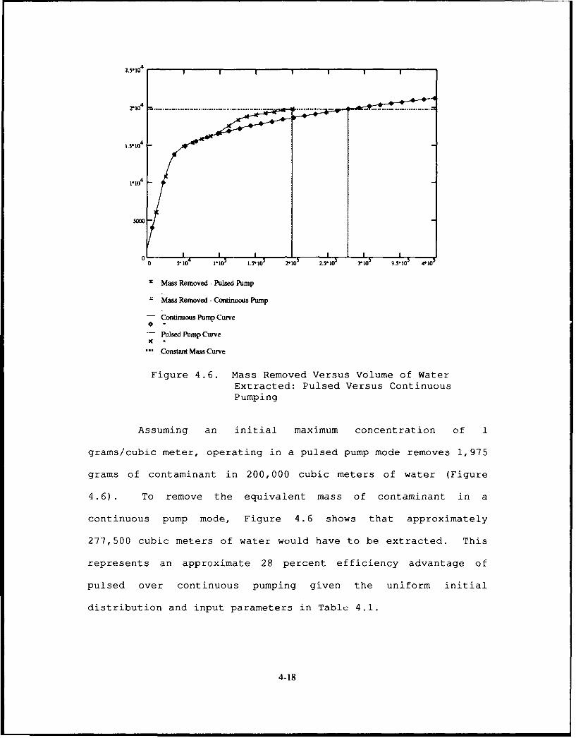
r14
I.S104 -
1.104
50W~
0 5le *1. 1Sjo' _O - 3.'L0 3.5! 10 4*105
r Mass Removed - Pulsed Pump
Mass Removed - Continuous Pump
- Continuous Pump Curve0
Pulsed Pump CurveC .
. Constant Mass Curve
Figure 4.6. Mass Removed Versus Volume of WaterExtracted: Pulsed Versus ContinuousPumping
Assuming an initial maximum concentration of 1
grams/cubic meter, operating in a pulsed pump mode removes 1,975
grams of contaminant in 200,000 cubic meters of water (Figure
4.6). To remove the equivalent mass of contaminant in a
continuous pump mode, Figure 4.6 shows that approximately
277,500 cubic meters of water would have to be extracted. This
represents an approximate 28 percent efficiency advantage of
pulsed over continuous pumping given the uniform initial
distribution and input parameters in Tablu 4.1.
4-18

The model demonstrates that operating in a pulsed pump
mode provides time for the slow desorption process to release
contaminant to the mobile water, thereby resulting in increased
concentrations of contaminant in the extracted water, thus
permitting higher removal of contaminant mass per volume of
extracted water. By operating in a pulsed pump mode, advantages
may include considerable savings in pumping and waste treatment
costs along with minimizing excess groundwater removal. To an
IRP program manager, this translates directly into dollars saved
by providing the 'biggest bang for the buck'. However, if
maximum contaminant mass removal is the IRP site remediation
objective, then this simulation indicates that pulsed pumpinq
will not remove more mass over time than continuous pumping, and
it appears that pulsed pumping may extend the duration of the
remediation efforts.
Continuous Pumpin. In this simulation, we demonstrate the
flexibility of the model by specifying arbitrary initial
conditions, thus allowing simulations to more realistically
depict an actual contaminated site remediation. During this
simulation, the pump is left on continuously for a total
duration of 100 days. The input aquifer parameters are the same
as those used in the previous simulation (Table 4.1) . The
layered diffusion model is used, and the initial contaminant
concentration distribution in the mobile region is entered as
discrete points as shown at Figure 4.7.
4-19

C0
n . 75 X XaC
nt 0. 5' X X Xr
tat• 0.25
0n
0 I I I I I I I I -
0.2 3.3 6.4 9.5 12.6 15.6 18.7 21.8 24.9 28
Radial Distance [m]
Figure 4.7. Initial Conditions for ContinuousPumping Simulation
The immobile region initial contaminant concentration
distribution was set constant at 1.0 (dimensionless) radially
throughout the aquifer (0.2-28.0 meters) and 0.0 at all other
locations.
As can be seen from Figure 4.8, the layered diffusion model
simulates the early breakthrough and long concentration tail at
radial distances 12.6 meters, 15.6 meters, and 18.7 meters where
the initial concentrations were 1.0 and at radial distances 21.8
meters and 24.9 meters where the initial concentrations were
0.75 and 0.5, respectively. Note that at radial distance less
than 9.5 meters, there is a slight increase in the solute
concentration with time. After this increase (which peaks at
various times for the various radial distances), the
breakthrough occurs and subsequently tailing at each of these
locations.
4-20

00
$4
C9)
ko4
'.4
oo
4')
'.44
0)0
04
410
44
r64
4-24

In order to more clearly see this peaking during the early time
period, we generated the effluent concentration profile for the
first 10 days at all radial locations (Table 4.7) and the
graphical representation (Figure 4.9).
Table 4.7
Mobile Concentration Profile for the First 10 Days
Day Radial distance starting at the well [m]
0.2 • 3.3 6.4 9.5 12.6 15.6 18.7 j 21.9 24.9 28.0
0 .5000 .5000 .5000 .7500 1.000 1.000 1.000 .7500 .5000 .00001 .4794 .4955 .6063 .8344 .9710 .9742 .9220 .6862 .4158 .02362 .5421 .5786 .7068 .8685 .9430 .9366 .8489 .6192 .3461 .02463 .6351 .6700 .7715 .8741 .9131 .8912 .7788 .5526 .2871 .02114 .7084 .7342 .8027 .8639 .8799 .8407 .7112 .4884 .2369 .01735 .7509 .7677 .8103 .8443 .8427 .7870 .6458 .4277 .1944 .0139"6 .7678 .7781 .8027 .8183 .8016 .7316 .5828 .3715 .1587 .01117 .7824 .7882 .8011 .8032 .7730 .6897 .5336 .3271 .1297 .00748 .7878 .7906 .7949 .7860 .7432 .6485 .4873 .2872 .1043 .00519 .7865 .7870 .7844 .7656 .7114 .6072 .4433 .2509 .0828 .0036
10 .7802 .7788 .7703 .7427 .6783 .5665 .4019 .2180 .0654 .0027
Given the initial contaminant distribution (Figure 4.7),
this peaking of highly contaminant water is transported inward
toward the well the moment the well is turned on. Since we have
assumed radial flow this sudden change generates this slight
increase and surfaces as time progresses. This behavior appears
to make physical sense and therefore is plausible that this
simulation is depicting the physics that could be occurring in
the aquifer.
Moide VArifiaationi/Comparison
The basis for model verification was to compare this model
with existing models formulated using the same
4-22

0V
$4
.)0
00
In
V4 064.4
934~
0100) ,
01 X
64.0
544
oQ.4.)
,0
44 >
In 01
0))
-A 00C-)4
0 in
412
4-23

sorption/desorption assumptions. In Chapter II we reviewed the
literature related to modeling sorbing solute transport. The
review focused on analytical models describing converging radial
transport and incorporating equilibrium or rate-limited
sorption, with the rate-limitation described by either a first-
order equation, or by Fickian diffusion in immobile regions of
an aquifer. In addition, we searched for any independent
modeling efforts in the area of pulsed pumping.
The literature search uncovered various researchers who have
presented analytical models that met the above criteria. For
purposes of comparison, the analytical model presented by Goltz
and Oxley was used (Goltz and Oxley, 1991]. Their model solves
the same sorption/desorption equation set for the pump on used
in this research. However, their model does not allow for
arbitrary initial conditions or pulsed pumping. Finding no
analytical pulsed pumping models, the literature was searched
for numerical models using the same criteria as above.
A numerical model by Huso was found that used the Finite
Element Method and Finite Difference Method [Huso, 1989] . In
this model, the pump on expression governing contaminant
transport within the mobile region (Equation (3.1)) and Fick's
second law of diffusion (Equation (3.14)) for spherical and
layered immobile region geometry were incorporated. Huso's
model allows for arbitrary initial conditions, multiple radial
locations, and simulates pulsed pumping by using a small pumping
rate. However, Huso's pulsed pumping simulation does not
4-24

explicitly include the governing contaminant transport equation
when the pump is off (Equation (3.67)).
The test consisted of running the Goltz/Oxley model and Huso
model and comparing simulations with simulations of the model
presented in this research. The input parameters presented in
Table 4.1 were used for all three models. With identical input
data, all three models should produce similar results. However,
some deviation will be expected since the analytical models
solve for the mobile concentration for all time simultaneously,
while the numerical model steps forward in time; thus, the
numerical model is subject to compounding errors [Huso, 19891.
Simulation parameters consisted of cycling the pump on and
off at 100 day intervals for a total duration of 400 days. The
initial mobile and immobile contaminant concentration
distribution was set constant at 1.0 throughout the aquifer
(0.2 - 28.0 meters) and 0.0 outside the aquifer (beyond 28
meters).
Figure 4.2 shows the simulation at multiple radial locations
for the model presented in this research operating in a pulsed
pump mode. Because of data and design limitations with the
other two models, the comparison test was conducted at the well
only. Unfortunately, since the Goltz/Oxley model only permits
pump on operation, data only exists for the first 100 days for
that model. In addition, only selected data points in time were
available for Huso's model. Table 4.8 shows the effluent
4-25

concentration profile comparison at the well, and Figure 4.10
shows the graphical representation.
Table 4.8
Layered Mobile Region Comparison Test
Day Goltz Huso Model Day Goltz Huso Model10 1.001 1.001 .9999 210 - .18 .172820 .9937 .9937 .9936 220 - .16 .156430 .6750 .6750 .6750 230 - .12 .097940 .2978 .2978 .2978 240 - .08 .057650 .1463 .1463 .1464 250 - .04 .044960 .1045 .1045 .1045 260 - .04 .041270 .0906 .0906 .0906 270 - .04 .039280 .0816 .0816 .0816 280 - .04 .037790 .0739 .0739 .0738 290 - .04 .0364100 .0673 .0673 .0673 300 - .04 .0353110 - - .0932 310 - - .0497120 - - .1016 320 - - .0552130 - - .1140 330 - - .0630140 - - .1272 340 - - .0714150 - .14 .1398 350 - .08 .0797160 - - .1516 360 - - .0876170 - - .1625 370 - - .095118- - .1726 380 - - .102219- - .1822 390 - - .1090200- .20 .1911 400 - .12 .1156
1.2 --
n --Model
C0.8
C
nt 0.6ra 0.4ti0 0.2
0 2 4 6 8 10 12 14 16 18 20 22 24 26 28 30 32 34 36 38 40Time [ X 10 days]
Figure 4.10. Effluent Concentration Profile Comparison atthe Well When Sorption/Desorption isControlled by Diffusion Within LayeredImmobile Regions
4-26

As can be seen from Table 4.8 and Figure 4.10, the model
presented in this thesis tracks very close to the Goltz/Oxley
and Huso models. As Figure 4.10 demonstrates, all models
initially show a high removal of contaminant until tailing
appears around day 50. From this point to day 100, the tail
appears and reaches a residual concentration. At day 100, the
well is turned off and the mobile concentration rises, as
contaminant in the immobile region slowly desorbs into the
mobile region. At day 200, the well is turned on, and again the
breakthrough and tailing is observed. At day 300, the well is
turned off, and expectedly, the mobile concentration rebounds.
At the end of the simulation (day 400), the levels in the
immobile regions are still quite high (Table 4.6) which
indicates only a portion of the total contaminant was removed
during this 400 day simulation.
Although favorable comparison results with both models
during the first 100 days, deviations are apparent with the Huso
model at certain data points. As previously mentioned, one
possible explanation for this deviation is that the numerical
model steps forward in time; thus, the numerical model is
subject to compounding errors. Another possible explanation for
this deviation could be that Huso's simulations are based on a
finite element and finite difference method which approximates
the equation set. Still another possible explanation could be
that the model presented in this thesis uses numerical
4-27

approximations, such as numerical integration, which could
explain the difference in results.
4-28

This concluding chapter draws together the research
presented in the previous chapters. It begins with an overview
of the research effort. Next, it summarizes the findings of
this study, and finally, it lists recommendations for model
improvements and for follow-on research.
The focus of this research was to model the fate and
transport of contaminated groundwater under certain simplifying
assumptions. It was intended that our research would assist
Installation Restoration Program (IRP) managers to estimate the
level and type of aquifer cleaniup effort. As such, the main
thrust of the research was to analytically model contaminant
transport and show how the rate-limited sorption process
influences the fate of contaminants in porous media. With
recent criticisms of pump and treat remediation, primarily due
to its inability to account for rate-limited sorption and
desorption, our research was tailored to account for This
behavior. Specifically, it incorporated one method that has
been proposed to enhance typical pump and treat remediation:
pulsed pumping.
The literature review clearly revealed that research during
the last few decades has contributed to a better understanding
of the transfer of solute in porous media through the mechanisms
5-1

of rate-limited sorption and desorption. There appears to be an
increase in mathematical models focused on contaminant transport
and rate-limited sorption/desorption. However, chere does not
appear to be many computer-based analytical models that
incorporate rate-limited sorption/desorption and none that
include pulsed pumping.
In this research an analytical model was formulated based
upon solutions governing the transport of a contaminant during
aquifer remediation by pulsed pumping. Contaminant transport
was assumed to be affected by radial advection, dispersion, and
sorption/desorption. Sorption was modeled assuming equilibrium
or rate-limited, with the rate-limitation described by either a
first-order equation, or by Fickian diffusion of contaminant
through layered, cylindrical, or spherical immobile water
regions. The model equations were foemulated using an arbitrary
initial distribution of contaminant in both the mobile and
immobile regions and were analytically solved in the Laplace
domain. These analytical solutions were then numerically
inverted and converted back to the time domain.
Summary of Findinan
Simulations were used to demonstrate the capability of the
model. In addition, a comparison of this model's simulations to
other models was conducted with favorable results.
Unfortunately, time constraints precluded a thorough evaluation
5-2

of the model. However, the model simulations that were
conducted revealed the following:
(1) A pulsed pump operation may allow for more efficient
contaminant removal in a groundwater remediation project. The
model demonstrates that operating in a pulsed pump mode provides
time for the slow desorption process to release contaminant to
the mooile water and eventually allows the system to approach
equilibrium.
(2) The pulsed pump simulation showed increased
concentrations of contaminant in the extracted water indicating
a higher removal of contaminant mass per volume of extracted
watei.
(3) The simulation indicates that pulsed pumping does not
accelerate the cleanup time but can achieve approximately the
same concentration levels of contaminant as continuous pumping.
This may result in Fvings in pumping and waste treatment costs.
(4) The model was designed to provide flexibility by
allowing arbitrary initial contaminant concentration
distributions. Unfortunately, model simulations were limited
and a thorough assessment of this aspect of the model still
needs to be accomplished.
(5) A comparison test was conducted with existing models
found in the literature. Goltz and Oxley presented an
analytical model based upon the same sorption/desorption
assumptions used in this research for a continuously operating
5-3

extraction well [Goltz and Oxley, 1991]. Huso presenLed a
numerical model using the same sorption!aesorption assumptions
[Huso, 19892. The model compares favorably with the Goltz/Oxley
and Huso models.
2m29akbtiona
As discussed in Chapter I, the development of an analytical
model requires simplifying assumptions in formulating the
equation sets. Therefore, the primary emphasis for future
research is to relax or eliminate these assumptions. More
specifically, emphasis should be focused in the following areas:
(1) Include drawdown of the aquifer water table as part of
the equation set formulation. This would reflect a more
realistic scenario.
(2) Eliminate the necessity for radial symmetry. That is,
develop a mathematical model that is truly two dimensional or
three dimensional.
(3) Include an arbitrary groundwater velocity field or
hydraulic gradient.
Other model applications could include:
(1) The pumping schedule could be optimized so that a
greater amount of contaminant can desorb from the immobile
region. In this model, the pump off time was arbitrarily
selected.
(2) Extend the capability of the model by including
multiple wells, including injection wells. Again, optimizing
54

the number of wells and cycling periods would provide a better
simulation of a real contaminated site.
(3) Add the ability to estimate the contaminant mass
remaining in the aquifer. Knowing this information will show
the efficacy of an aquifer remediation effort.
5-5

Appendicx A: A Green's Function Aproach to
Anal-tical Modeling Aajifer Decontamination by Pulsed Pu12•ing
With Arbitrary Initial Conditions
This appendix presents the theoretical development and
detailed mathematical analysis of the equations and solutions
that govern sorbing solute transport. The derivation uses
arbitrary initial conditions and is developed based on the five
expressions of sorption/desorption (equilibrium, two-region
first-order rate, and Fickian diffusion of rectangular,
cylindrical, and spherical immobile region geometry) for
conditions when an extraction well is on and when an extraction
well is off.
The mathematical representation of the advection and
dispersion that govern dissolved transport of a single
contaminant in saturated, homogeneous porous media with radial
converging flow is
aC' (r,t) 0 1 a aC (r,t) 1 C (r, t)- r(Dm(r) + D) M) Vn(r) (A.1)rt r L or ar
where D' is the dispersivity [L] of the porous media and D' is
the molecular diffusion coefficient [L! / T]. If we include a
sink term to describe the transfer of contaminant from the
aqueous phase to immobile water regions, and account for the
distribution of contaminants between aquifer solids and the
groundwater (Rm = I + (pKd) 0 0.) , then Equation (A.1) becomes
A-I

aC' (r, t) (r t)aC- L D r + D ') 'C' t)a~t Rr ar M oh"
(A.2)V. (r) a)C'. (r, t) 0•=,Rim a9C. (r, t)
R a- OmRm at
f we define
D' = aiVm(r) (A.3)
-- R(A.4)OmRm
then Equation (A.2) becomes
aC'(r,t) _ -l m[(aiVm(r) + rD,)aC(r,t)]at Rmr D~r 0
(A.5)V. (r) tgC" (r, t) a3(C" (r, t)
Rm "r at
or
°aC'(r' t) I a~ mor•[ a Vm (r) + atC' ( r, t)ro"
(A.6)Vm (r) aC.' (r, t) D C'm (r, t)
R. ar i1 at
If we substitute Equation (A.3) into Equation (A.6)
aC' r, t) _ aC (rt)ac•(rt) R- [ a, Vn (r) + D') .C-(r,t)
(A.7)
,Vm (r) aC" (r, t) aC' (r, t)
Rm Ar at
A-2

and define
Dm = a, IVm (r)I (A.8)
then Equation (A.7) becomes
aC' .(r, t) =I a [(D,. +D) •C(r, t)
(A.9)V, (r) aC' (r, t) W'• (r, t)
Rm n P t
where Dm is the mobile region dispersion coefficient [L2 / T].
Equation (A.9) describes the transport of a single sorbing
solute in saturated, homogeneous porous media. Mathematical
modeling of this phenomena often incorporates simplifying
assumptions, depending on whether an extraction well is on or
off.
Model Formulationa Extraction Wall On
In the case where we have an extraction well operating, it
is •ften assumed that the mobile region dispersion coefficient,
Dm, is much greater than the molecular diffusion coefficient,
D'. Thus, D' is considered negligible sufficiently close to
the well where the advective process due to the pump's influence
overwhelms the molecular diffusive process [Valocchi, 1986:1694;
Goltz and Oxley, 1991:548]. When this assumption is made,
Equation (A.9) becomes
A-3

aC' (r t D.aCm (r, t) V. (r) Wm'(r, t) c)C (r, t)
SP(A.10)COt R. 0r R.. r &t
which describes the transport of a single sorbing solute in a
radially flowing aquifer in a porous medium with immobile water
regions [Goltz and Oxley, 1991:548]. The dependent variable in
this equation, C , represents a volume-averaged solute
concentration within the immobile region defined by [Goltz and
Oxley, 1991:548]
C'(r,t) = z-• C'(rz,t)dz (A.11)im 0 a
If the depth or thickness of the aquifer region is b [L] and an
extraction well is present pumping at a rate Q, [L / T], with
the mobile region dispersion coefficient, D., given by
Dm(r) = a, V(r)I (A.8)
then the radial velocity is
V(r) - Q" (A.12)2 bO..r
We now seek a dimensionless fori. of Equation (A.10). Thus, we
develop dimensionless variables. If we define
X = C, r (A.13)
T = C2 t (A.14)
Cm(X T) - C(r,t) (A.15),0
A-4

Ci.(X, T)- i C'(,t (A. 16)
C0
where X is the dimensionless radial distance, T is the
dimensionless time, Cm(XT) is the dimensionless mobile region
solute concentration, C• (X,T) is the dimensionless volume-
averaged immobile region solute concentration, C1 and C2 are
constants, and C' is some initial maximum concentration of
C'(r, t = 0) and C'(r, t = 0) between the well radius, rý [L], and
the radius of the initially contaminated zone, r. [L]. Then
C'(r, t) = C' X C. (X, T) (A.17)
C'(r, t) = C , = C1 1 (X,T) (A.18)
and
W' (rt) - c" DCm (X, T) LT cd = Cm (X, T)
0 -Y (q) (A.19)
aC'M(rt) - C" Cm(X'T) dX =C" Cmn (X, T) (C
%0 0P o( 1 (A.20)
M aC,. (r, t) _ [ C"(rt). dX C" (X , T) ( 2)
2 a O[r Idr 0i 2CIC (A.21)
aC" (r, t) = mC (X, T) dT - C,,n (X, T) (A.22)
a 0 a" dt 0 (o2
A-5

Substituting these expressions into Equation (A.10) gives us
? W. (X, T) D. -2rc, 2C (X, T) Vr((r) C., W.m (X, T)C2 ['Y Rm 0 X2 Rm 0 X
(A.23)
SCP i (X , T )
Dividing each term in this equation by C2 and C' yields
aCm(X,T) _Dm C12 a 2Cm(XT) V (r) C, WCm(XT)
R, C2 Rm C2 X
(A.24)
-I (X, T)aT
Recall that
Dm,, a, IVm (r)I (A.8)
V( - Q. (A.12)
2 2ibbOr
Substituting these expressions into Equation (A.24) produces
Cm (X, T) = a1Q-C,3 2Cm (X, T) + QWC 12 m(X, T)
)T 2nbOm XR.C2 C X2 2tbOmXRmC 2 aX
(A.25)
_ Cj (X, T)aT
In order to determine C, and C2 uniquely, we seek a second
equation. In Chapter 2, we discussed how the transfer of solute
between mobile and immobile regions may be assumed to be
A-6

governed by Fickian diffusion of solute within immobile regions
of specified geometry (Goltz and Oxley, 1991:548-549].
Mathematically, Fick's second law of diffusion describing
contaminant transport within immobile regions is
aC' (r, z, t) =D" a C (r, z, <tz)
Rim 0 < z < a (A.26)
If we define
Z = C3 z (A.27)
C: (r, z, t)C, (X, Z, T) = r (A.28)C0
where Z is the dimensionless immobile region variable,
Ca(XZ,T) is the dimensionless concentration at points within
the immobile region, and C3 is a constant, then
C(r,z,t) = T C.(XZ,T) (A.29)a:rzt = C1 C,'C3'1C2
and
•C(r,z,t) W .Ca (X, Z, T) dT C. (X, Z, T)c3CIP C (C, (A.30)at 0 T dt 0 aT
aC(r,z,t) WC (X, Z, T) dZ WC. (X, Z, T)dz (r (C 3 ) (A.31)
az 0Z dz 0 )z
A-7

Substituting these expressions into Equation (A.26) gives us
"IC. (X, Z, T) _C __X, Z,___T_
(A.32)
or
R=C.C2 ((X, Z, T) _ D' a2[Z•_ •Ca(XZ,T)R_- Z-' CoC3L2 _ Z (A.33)
where Equations (A.32) and (A.33) are defined over the interval
0 < Z < a. Dividing each term in this equation by Run C, and
C 2 yields
DC.(XZ,T) _ D C32 1 ± Zui •C 1(X,Z,T) 0 < Z <a
0T Rim C 2 ZIU-1 aZ. Z I
(A.34)
We now seek the constants C, and C2 in Equation (25) such
that
a , Q . = 1 (A.35)
2 lbtmR.C 2
and
Qw C 2QW, = I (A.36)
2 ibOnR. C 2
A-8

Solving C2 in terms of CI in Equation (A.36) yields
QW C 12C2 = b R (A.37)2 nbe.R.
Substituting Equation (A.37) into Equation (A.35) gives us
a, Q" C13 (2 7bOmRm) =1 (A.38)
2xbO.Rm QCI2
or
alC 1 =1 (A.39)
Thus,
C -(A. 40)a,
Substituting Equation (A.40) into Equation (A.37) results in
C2 2_ _R_ 12 (A.41)2 xbO Rmn al 2
Therefore, Equations (A.13) and (A.14) become
r
S=- (A.42)a,
T= Q,,t2T bOmRma 2 (A.43)
We now select C3 so that when z = 0, Z = 0 and when
z = a, Z = I That is, we want to normalize Z so that it
A-9

exists in the interval 0 < Z < 1. Therefore, Equation (A.27)
becomes
zZ -(A. 44)
a
where
C3- (A. 45)a
Using Equation (A.25) together with Equations (A.40) and (A.41)
results in the dimensionless form of Equation (A.10):
Cm(X, T) _ l O2 C•(X, T) + I CW(X, T) aC)(X, T) (A.46)
aT X aX2 X DTX GT
Taking the Laplace transformation of Equation (A.46) and
suppressing the (X, s) notation where S is the Laplace transform
variable results in
DCxj 2C +. -~a)L aP A7)
or
1 a2m 1! acsCm - C.(X,T = 0) +- +
X aX 2 X ax(A.48)
- [[sC - C• (X, T = 0)]
where Cm(X,s) is the Laplace domain dimensionless mobile region
solute concentration, CUm(X,s) is the Laplace domain
A-IO

dimensionless volume-averaged immobile region solute
concentration, and S is the Laplace transform variable.
After describing remediation of a cylindrical contaminated
area of extraction well radius r., radius of contamination r.,
and defining X. = r / a, and X. = r / a, as the
nondimensionalized well radius and contaminated area radius,
respectively, the following initial and boundary conditions can
be formulated for the various models [Goltz and Oxley, 1991:549-
550; Valocchi, 1986].
Initial-Conditions:
Cm(X,T = 0) = Fm(X) X. < X < X. (A.49)
C,(X,T = 0) = F,(X) X" < X < X. (A.50)
Cn(X, T = 0) = C,(X, T = 0) = 0 X > X. (A.51)
where Fm(X) and F=(X) are dimensionless arbitrary initial
concentration conditions in the mobile region and immobile
region, respectively. The diffusion models require tne
following addicional initial conditions to describe transport
within the immobile regions [Goltz and Oxley, 1991:549-550]:
C.(XZ,T = 0) = F1(X,Z) Xw < X < X. (A.52)
C.(X, Z, T = 0) = 0 X > X. (A.53)
where F (X, Z) is the dimensionless arbitrary initial
concentration condition in the immobile region of a certain
geometry. Again, Equations (A.49), (A.50), (A.51), (A.52), and
A-1l

(A.53) state the initial conditions, which assumes contamination
of mobile and immobile regions at some arbitrary concentration
within a cylindrical region of dimensionless radius X..
Boundary Conditions:
C.(X.,T) + -C (X.,T) = 0 (A.54)aX
-C (Xw, T) = 0 (A.55)
The diffusion models require additional boundary conditions •o
describe transport within the immobile regions of certain
geometry.
aJc,
57 k X, Z = 0, T) = 0 Xý < X (A.56)
Ca(X, Z = 1, T) = Cm(X, T) Xw < X (A.57)
Equation (A.54) states that the total mass flux inward at the
outer boundary (X = X.) must always be zero, since initially,
there is no contaminant mass at X > X.. Equation (A.55) states
the boundary condition at the well radius and is based on the
assumption that at any time, the concentration inside the well
bore is equal to that entering the well from surrounding media
[Goltz and Oxley, 1991:549]. This implies a zero concentration
gradient at the interface between the well and its immediate
adjacent aquifer. Equations (A.56) and (A.57) state that the
concentration within an immobile region of certain geometry is
A- 12

zero at the center and is equal to the mobile region
concentration at its outer boundary.
Now that we have established the governing differentiAl
equation (Equation (A.46)) and the initial conditions and
boundary conditions, we will now go through the mathematical
formulation for each model.
Local Eauilibri,--Modal (LXA%. From Equation (A.46), if
is defined to be zero, ard if we suppress the (X,T) notation,
then Equation (A.46) becomes
__m I ia2C Iac.-Cm _ 1C +-(A.58),T X aX2 X aX
and Equation (A.48) becomes
SCm - Cn(X,T=0)= + (A.59)x a•x 2 X ax (.9
Rearranging this expression and multiplying each term by X
gives us
a2 + XsCm = --XC (X, T 0) (A.60)aX2 aX
If we define
y -S (A.61)
and
F(X, s) = -XCm(XT = 0) (A.62)
A- 13

together with the initial condition Cm(XT = 0) = F.o(X)
then Equation (A.60) becomes
D2 + aC - XC. = F(X,s) (A.63)
First-Order Rate Modea. In Chapter II we introduced the
first-order rate model. That is, the transfer of solute between
the mobile and immobile region can be described using a first-
order rate expression:
iC (r,t) [C' (r, t) - C' (r, t)] (A.64)_)t O R Mii
We seek a dimensionless form of Equation (A.64) . Recall
Equations (A.4), (A.15), (A.16) (A.42), and (A.43)
---- (A .4)
OmRm
C.(X,T) = (r, t) (A.15)C0
Ci•n(X, T) = mC, (Ar't)C,0
r
- (A.42)a,
T Q"t (A.43)2 ibOmRa,
2
Rewriting Equation (A.64) into dimensionless form, term by term,
yields
A-14

aC r, t)C (X, T) dT C a (X,T) fQ .A.650 CT dt = 0 2-,2abO a 2 Ra 2ARm
where
C'(r, t) = C .Cm(XT) (A.66)
C' (r, t) = C" C=(X,T) (A.67)
Substituting these expressions into Equation (A.64) gives us
CC a(X, T) Q. a [C. _( '"C o 20T2 2-, CmaX2• CT).Cm(XT)] (A.68)
or
ac n (X , T ) _ j 27tbO :al2R m aL I C '[C .(X ,T ) -C ,. (X ,T)](A .9)0 Q - Q , c O nRun 0[•CT • X ) A
Thus,
c(X,T) [C (X, T) - C • (X, T)] (A.70)C)T Q .P
If we define the dimensionless first-order rate constant a as
a• 2 irba12
a d (A.71)Q.3
then Equation (A.70) becomes
acmjXT) = a[Cm (X, T) - Ci (X, T)] (A.72)
A- 15

Taking the Laplace transform of Equation (A.72) and suppressing
the (X,s) notation yields
L~- (a= - ci1) (A. 73)
sC - Cn (X, T = 0) = a(Cm - Cm) (A.74)
and solving for CZ in terms of Cm gives us
- = C. (X, T = 0) + aCm (A. 75)
Inserting this expression into Equation (A.48) results in
s?. -C.(X,1T = 0) = + X X- + in C(X, T = 0)
(A.76)
- PS Ci (X,T = 0) + Cm
- ~sL s + a S
and rearranging, collecting similar terms, and multiply each
term by X gives us
a2Cm acr XC'1S += _XCm(XT = 0)ax---2 ax s +----
(A.77)
+ XC ( X,'T = 0) PSso •
If we define
y' = sI + Pa (A.78)
A-16

and
F(X, s) =-X[C. (X, T = 0)- Ci (X, T =)[1s -)(s + a (A 79)
or
F(Xs) = -X[Cm(XT 0) + kCn, (XT = 0)s (A.80)IL s+a I
together with the initial conditions Cm(XT = 0) = Fm(X) and
Cn(X,T = 0) = Fi.(X) we get
F(X,s) X X(Fm(X) + IOaFm,(X)) (A.81)
So, Equation (A.77) becomes
a2Z .+ ac. Xy?ý = Fý(X,S) (A.82)aX2 ýX-
Diffusion Modals. As previously discussed, the transfer of
solute between the mobile and immobile regions may be assumed to
be governed by Fickian (Fick's second law) diffusion within
immobile regions of specified geometry (Goltz and Oxley,
1991:548-549]. Mathmatically, Fick's second law of diffusion
describing contan .nant transport within the immobile region is
aCC (r, z, t) _D" a azC_ OC(r, z, t)•R - - U C1 a 0 < z < a (A.26)ii t z U-1 az ( az
Recall Equation (A.34) which is the dimensionless form of
Equation (A.26):
C._(X,Z,T) _ D' C32 1 a F W 3C(X,Z,T)T _D C 2 3 _ a1 0 < Z < a (A.34)
0T Ri C2 Z L jz
A-17

If we substitute in Equations (A.41) and (A.45) then Equation
(A.34) becomes
._ D; 27b~mRma,2 1 0 aC 0 < Z < I (A.83)
SRim Qw a2 zu-1 ZZ
If we define a dimensionless immobile region solute diffusion
coefficient, De, as
D'a 2 2 7bO.R.= a2 QER2 (A.84)
Then Equation (A.83) becomes
C. (X, Z, T) = D. a [ZU_ C1 . (X, Z, T) 01< Z<I (A.85)aT T--7 -5Z DZ
and is valid for all the diffusion models. That is, u = 1, 2,
and 3 Now we take the Laplace transform of Equation (A.85)
using Equation (A.52) (initial condition) and Equations (A.56)
and (A.57) (boundary conditions)-
C.(XZ,T 0) = F.(X, Z) X., < X < X. (A.52)
~a(X, 0, T) =-0 0 < X < X. (A.56)az
C.(XZ = 1,T) = Cm(XT) X, < X < X. (A.57)
So,
= L ZS-a1 Z U Z (A.86)
A-18

sC-C. (X, Z, T=0) D, (A.87)
.- (X, Z) D Z_• aC. (A.88)z 'j1 az az)
thus
Dý a Z U-'• -s.=- (XZ) (A. 89)
where C,(X, Z,s) is the Laplace domain dimensionless
concentration at points within the immobile region. The
boundary conditions associated with Equation (A.89) are derived
by taking the Laplace transform of Equations (A.56) and (A.57).
Thus,
--a (X, Z = 0, s) = 0 X" < X < X. (A.90)az
C1 (X, Z = 1, s) = Cm(X, S) X, < X < X. (A.91)
We seek the general solution to Equation (A.89) using the
boundary conditions (A.90) and (A.91) for cases of v = 1, 2,3
(layered, cylinder, and spherical geometry, respectively). That
is, we seek
C. = C., + C.P (A.92)
where Ca is the general solution to the differential equation,
C.c is the complementary solution to the homogeneous
differential equation, and C.,P is the particular solution to the
A- 19
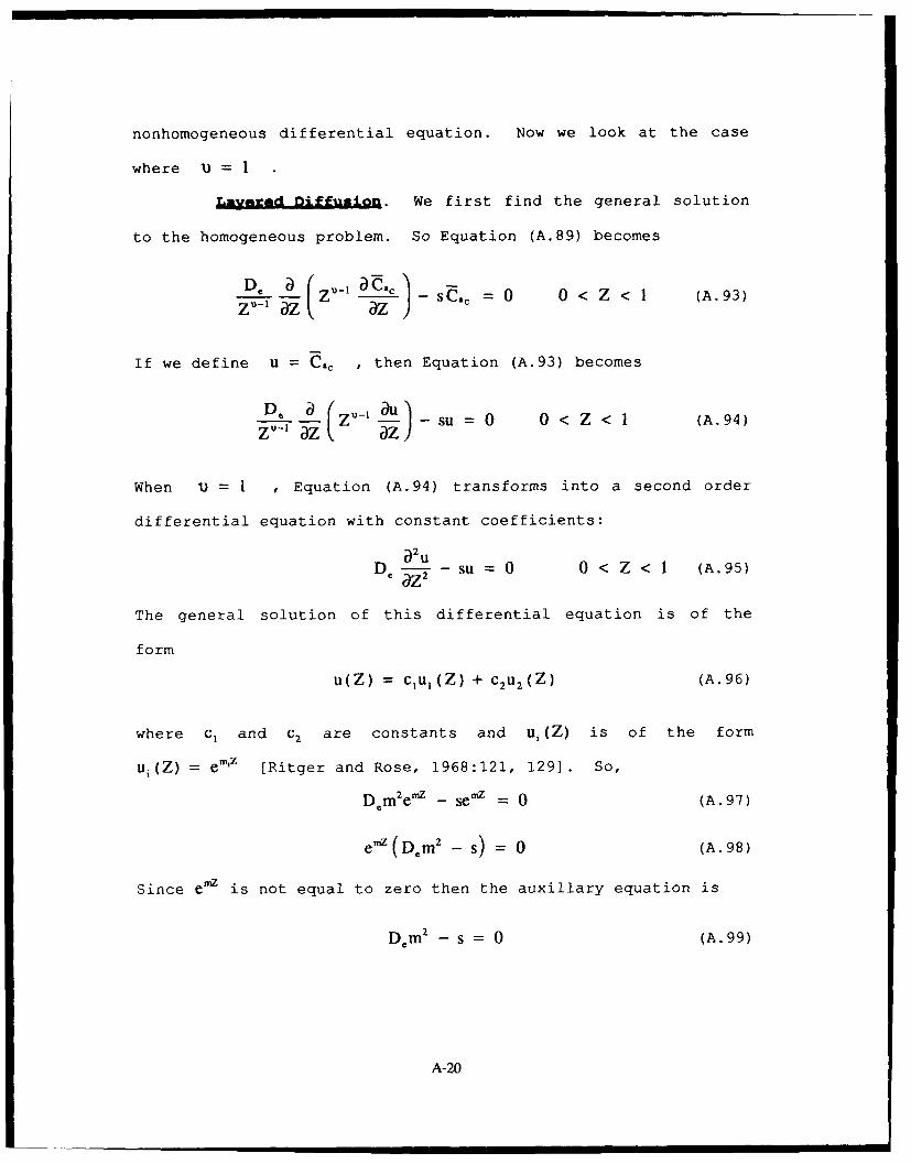
nonhomogeneous differential equation. Now we look at the case
where 1) = 1
Layared DIffusion. We first find the general solution
to the homogeneous problem. So Equation (A.89) becomes
D 'U- Z_ -C1c sCC =0 0 < Z < I (A.93)
If we define U = C. , then Equation (A.93) becomes
De a - -a -- SU = 0 0 < Z < I (A.94)
When 1 = I , Equation (A.94) transforms into a second order
differential equation with constant coefficients:
2uD -aZ2 su =0 0 < Z < I (A.95)
The general solution of this differential equation is of the
form
u(Z) = clu 1(Z) + c 2u2 (Z) (A.96)
where C, and c2 are constants and uj(Z) is of the form
uj(Z) = emiz [Ritger and Rose, 1968:121, 129]. So,
D m2 enz - sez = 0 (A.97)
e' (D.m2 - S)= 0 (A.98)
Since e is not equal to zero then the auxillary equation is
Dm 2 - s = 0 (A.99)
A-20

So,
m or m =m2 =A.j100)D,
Thus,
u(Z) = cAe + c 2e (A.101)
If we define
(A. 102)
then
u(Z) = Ce0 + c 2e-Q)Z (A.103)
We now check this solution for linear independence to
determine if Equation (A.103) is the general solution to
Equation (A.95). Thus, we use the Wronskian, W[u), u). That
is, if W[ul, u 2] * 0 then the two solutions, u, and U2 , are
linearly independent and u(Z) is the general solution. Using
Equation (A.103) with U1 =ez and u 2 = e-Jz we get
Ul U2 eoz e-,,z
W[u1 , U2] = (A.104)•u (oewZ - -(C-)ZUf U2 ~ M
= -Oe- eOz -OeO e-O = (-o- (o = -2 •o 0 (A.105)
Thus, U, and U2 are linearly independent so u(Z) = clez + c 2 e-Mz
is the general solution.
A-21

Now we seek the particular solution using a Green's
function. If we define U = C, then from Equation (A.89), we
have the following nonhomogeneous differential equation:
a2UD -•- sU = -F.(X, Z) (A.106)
with boundary conditions
aZ (Z 0) 0 (A.107)
U(Z = 1) = 0 (A.108)
Rewriting Equation (A.106) gives us
_2U 1
au = - D-- F.(X, Z) (A.109)•Z 2 De
or
S- 0)2U = -I F.(X, Z) (A.110)aZ2 D e
where (02 = s / D. (Equation (A.102)). We know the general
solution of this equation is of the form
U(Z) = AUI(Z) + BU 2(Z) + Up (A.111)
where A and B are constants and Up (or C?,) is the particular
solution (Ritger and Ross, 1968:438]. Based on the homogeneous
solution, we know that U (z) = cle z + c2e-(z satisfies the
boundary condition aU,(Z = 0) / aZ = 0 That is,
cWe (°) -0)2e-w(°) = 0 , which implies C, = C2 So,
A-22

U, (Z) = cieo + ce-0 (A.I12)
If we choose C, = 1 / 2 (without loss of generality), then
U,(Z) - = cosh aJZ (A.113)2
We also know that U 2 (Z) = c3e• + c 4e•z satisfies the other
boundary condition U 2 (Z = 1) 0 Thus,
U 2 (Z = 1) = 0 = c 3e'(1) + c4e-o(1) (A.114)
so
C4 -c 3e (A.115)
Therefore,
U 2 (Z) = c 3ez - c3e2c e-wz (A.116)
= c3eo[e e-° -e0 e0-] (A.117)
=C~edOI [em(Z1) - e(-O$~) (A.118)
or
U 2 (Z) = c3ew[-ei)(I-z) + e-)(I-z) (A.119)
Since c3e- is a constant, let's choose it to equal -1 / 2
(without loss of generality). This gives us
U 2 (Z) = 2 sinh c( - Z) (A.120)2
A-23
We now check to see if we have a trivial or non-trivial
solution using the zero boundary conditions for the homogeneous
case:
-(Z 0) 0 (A. 121)
u(Z = 1) = 0 (A.122)
This will determine the form of the Green's function for the
particular solution. We know Equation (A.110) with the above
boundary conditions has a unique solution if and only if the
homogeneous problem (Equation (A.95)) has only the trivial
solution for the same zero boundary conditions [Ritger and Ross,
1968:439]. Recall, u(Z) = Cie z + c2e- (Equation (A.103), so
S(Z = 0) = 0 = oxe - = (C 1 - c2, (A.123)
thus,
C, = C2 (A.124)
At the other boundary condition, u(Z = 1) = 0 , we get
u(Z = 1) = 0 = Cie + c2e-O41 i (A.125)
c 2e- = Ciet (A.126)
C2 -cie2o (A.127)
thus,
C1 = C2 =-cie 2a or c, = 0 (A.128)
A-24
so, u(Z) = 0 is the trivial solution.
Since we have a trivial solution we now construct the
particular solution using a Green's function which is of the
form [Ritger and Ross, 1968:440]
UI (Z)U 2 (0 Z < < Ip<;Ow(Ul, U21(0>
g(Z, ) = (A. 129)
UI (O)U2 (Z)p(C)w[ U1, U2](C)o <z
where W[Uj,U 2 ](ý) is the Wronskian of U, and U2 , and p(C) is
the coefficient of the first term in Equation (A.110) . From
Equation (A.110), we see that p(ý) 1. Now we determine the
Wronskian:
=IUIU 2 1 =_ cosh rOZ sinh (0(1I-Z)W[U1, U22 Uf Uf (o sinh wZ -(0 cosh (0(1 - Z) (A130)
= --o cosh co(1 - Z) cosh WZ - o sinh WZ sinhc0(1 - Z)
(A.131)
= -0[cosh (OZcosh (0(1 - Z) + sinh coZsinh w(1 - Z)]
(A. 132)
= -0o cosh((OZ + (0(1 - Z)) (A.133)
0- Ocosh 0O) 0 (A.134)
A-25

So,
cosh (oZ sinh (06 - Z < < 1
-0) cosh 0g(Z, ) = (A. 135)
cosh o sinho)(1 - Z-(o cosh 0)
Therefore,
Up Ca,(X,Z,s) = -J'g(Z,d) F[(X' )JdD (A.136)
Thus, Equation (A.92) is
Ca = Cac + C.p = A cosh OZ + B sinh 0)(1 - Z)
(A.137)
De
or
-- cosh WZ+Bsn ( )+ hCZ zsinh CO(I - ý)F.(X, C)dýCa = AcoshZ+ Bsinh)(- Z) +D cosh o
sinh0)(l - Z)oz+ -~~~ 'Ioh4F.(X,ýdo)D cosh 0)0
(A.138)
Now we apply the nonzero boundary conditions (Equations (A.90)
and (A.91))to find the constants A and B.
A-26

ac. (X, Z = 0, s) 0 = (A sinh 0(0) - (oB cosh 0o(I - 0)
+ Csinh CD(0) 1 sinh co(1 - C)F. (X, ý)dC+oD. cosh CO
_ cosh 0)(0) sinh 0)(1 - Z)F, (X, Z)0)D. cosh co Z= 0
-Co cosh •(0 - 0)• •osh(4) ,(,ýdODco cosh ( C
+ sinh (0 -0) cosh(coZ) F (X, Z)
caD, cosh o =
(A. 139)
or
0 -- oB cosh 0o (A.140)
So, B = 0 Now we apply the second boundary condition
C1 (X,Z 1, s) - C.(X, S)
S(X,s) = Acosh(o(1) + cosh W(1) Jsinh0o(_ -)F.(X, )dý(oDe cosh (0
(A. 141)
+ siih c(I1 - o)sh(4)M ioDcosh) h F((xo)d•
ZC. (X, s)So, A = Cos) O Thus, Equation (A.138) becomes
cosh Z o
h - g g(Z,) F. (X,C)d (A.142)
A-27

Combining Equations (A.48), (A.49), and (A.50) we get
I - 1 D - (X)] (A.143)sm- FT(x) x X + LS
Now we need an expression for Cm. Recall Equation (A.11):
C'z(r,t) = 1)z-C' (r, z, t)dz (A.11)
Normalizing and converting this equation to dimensionless form,
where Cn(X,T) = C'(r,t) / CQ (Equation (A.16)) and Z = z / a
(Equation (A.44)) we get
C'Cm,(X,T) f ( 1) Z(1)) C'C.dZ = UC'.,Z' C, dZ (A.144)
So,
C (X,T) = ZUI- C.(X, Z,T)dZ (A.145)10
Taking the Laplace transform of Equation (A.145) with 1 = 1
we get
i (X, s) (A.146)L C (X, Z, s) dZ(A 1 6
Substituting in Equation (A.142) into Equation (A.146) we get
A-28

C --X, s)--h_ -D-" g((Z,X)F. (X,)d (A. 14 7)
I.(~s Jcosh (0Z D, - L .rd](rd
c-os'-' €.0 I D-'-[" g (Z,ý) dZ ý.(X,ý) dý (A. 1498)cosh W) D..40
Cm.(X, S) [s;inh OZI IIIg(Z d MC)C (A. 149)
S s) cosh (o -I D g(Z, ý)dZ (X, ý)dý (A. 150)
Now we determine 0 g(Z, C)dZ where g(Z,ý) is defined by Equation
(A.135).
A-29

|zg ( coshI I s Iinh W 0
Jo[ -o -cosh o J(A. 151)
+ j1[coshw4sinh0)( - Z)
sinh o)Z siflh)000 ) ý cosh 0cosh0)(l- Z) 1
-sOD 2 cosh D 0 + - cosh(-) (A.152)
sinh O0 sinh co(l - cosh O3=+ 2
-- 0)2 cosh (0 cosh 0)(A.153)
cosh eo1 cosh co(1 - 0
O02 cosh w
( 1 2 cosh[co sinh 0 sinh CO(1-) + cosh C cosh O)( - )]
(A. 154)
cosh+2w02 coshc
2osh (A. 155)
(o2 cosh 0)O cosh
So,
IIg(Z, C)dZ = - _- cosh 0[I + (A. 156)
Inserting this equation back into CZ(X,s) (Equation (A.150))
gives us
C(X, s) = M s ) -1 wI+ Cosh (X, r)dr (A. 157)w cosh 0) w02D L cosh w I
A-30

Now we have an expression for C,(X, s). Using this equation
let's substitute it back into Equation (A.143):
sCm - Fm (x) = lam+ CF.x (X)f -X- +3[Sann - F. (X)] (A. 14 3)
Thus,
SmF. (X) +x ax 2 ax
RESClsinhCX - 2 1 T +cos h F. (o cosh O 0)2DD,, cosh '0 ' "
(A.158)
Rearranging this equation and multiplying each term by X gives
us the following
a2 + - - Xsý!(1 + Gsih (0 X[Fm(X) + OF.m(X)ax--+ax 0) cosh Ci =
+ P__S -1 + cosh ( x, ((02D L cosh 0)
(A.159)
If we define
Y = s(1+ 0sinhco(0 (A.160)
k. CO cosh (0
and recall that S = C 2D, (Equation (A.102)), then we get
ax- + a x = -,X[F.(X) + OF. (X)cOshýh( (A.161)
JOcoshfCO zJ _ o
A-31

The right-hand side of this equation can be further simplified
using the initial conditions C (X,T = 0) = Fi(X) (Equation
(A.50), C.(XZ,T = 0) = F.(X, Z) (Equation (A.52)), and the
dimensionless expression for the volume-average immobile region
solute concentration, C,.(X, T) LZU-IC. (X, Z, T)dZ where
) = I (Equation (A.145)). Therefore, at time T = 0
F (X) = C,1 (X,T = 0) = JC.(X, Z,T = 0)dZ = oF,(X,Z)dZ10 . (, Z) d (A. 16.2)
Putting this expression for F•(X) into the right-hand side of
Equation (A.161) gives us
-X[F. (X) + Pj"F. (X, Z)dZ + 0r[ cosh +(XC)dI (A.163).10 '0 Lco sh W J
or
-X[F.(X) + IJF.a(X, )dCZ + 01-1cos--- .31
(A.164)
Thus, Equation (A.164) becomes
-X[Fm(X) + 0 J1cosh(oK) F. (X, ý)dC] (A.165)cosh (o
So, if we define
F(Xs)= X[F.(X) + cosh(W4) F,(X, )d] (A. 166)I ~cosh c (
then Equation (A.161) becomes
a2 ZCm -C)X-- + X XCf = F(X, s) (A.167)
A-32

Using similar techniques as in the above derivation when 1=
, we now seek the solution when v = 2
C__lindrcal Diffunion. From Equation (A.85) we have
C(X, Z, T) = D a Z[z-I IC. (x z, T)] 0 < Z < 1 (A.85)
which is valid for all the diffusion models. As previously
derived, we now take the Laplace transform of Equation (A.85)
using Equation (A.52) (initial condition) and Equations (A.56)
and (A.57) (boundary conditions):
C.(X,Z,T = 0) = F.(X,Z) X,. < X < X. (A.52)
= 0,T) = 0 X, < X < X. (A.56)az
C.(XZ = 1, T) = Cm(XT) X. < X < X. (A.57)
So,
S- = iz-•(z 2-- (A.86)
Szýa - C.(X, ZT = 0) =-1- a(z1 acIJ (A.87)
sC. - F.(X.Z) - - Z (A.88)zv-1 az az}
Thus,
D, a (ZV_ o%.- sC. = _F.(X Z) (A.89)
with the following boundary conditions:
A-33

. (X,Z= 0, s) = 0 X, < X < X. (A.90)
Ca(X, Z = 1, s) = C=(X, S) X, < X < X. (A.91)
We seek the general solution to Equation (A.89) using the
boundary conditions (A.90) and (A.91) for case of v = 2
That is,
Ca = C., + Cap (A. 92)
where C1 is the general solution to the differential equation,
Cac is the complementary solution to the homogeneous
differential equation, and Cp, is the particular solution to the
nonhomogeneous differential equation. So for the case of
u = 2 , Equation (A.89) becomes
D. z az s = -(X,Z) (A.168)
Multiply Equation (A.168) by I / D. and differentiating the first
term gives us
I -z F (X, Z) (A.169)
or
I a2e ae] •e F.XZ1 Z-2 + SZD-(X, Z) (A.170)
Thus,
a2 C 1 a. s - F.(XZ)- + (A.171)aZ2 Z aZ DA D,
A-34

If we define
z=03Z (A.172)
W(a) = Ca(Z) = (A.173)
where 032 = S / D. (Equation (A.102)), then
ca aw dw- -- (0- (A.174)
0 ai dZ
)zz (A.175)
Substituting these equations into Equation (A.171) gives us
22W 02 aw F._(X,_) __ _ _))W2 2 2W = 0X _)- (A.176)aj2 i Z£ D. D.
Multiplying through by 1 / 1)2 yields
a2w + - Zw _ = 2 (A.177)b2 Z (0 • De
We now seek the complementary solution to Equation (A.177).
That is,
a 2W I aw' + W -- 0 (A.178)ai2 i Z£
which we know to be a modified Bessel function of order zero
[Abramowitz and Stegun, 1970]. Therefore, the general solution
to this homogeneous differential equation is
A-35

W(z) = CI WI (1 Z) + C 2W2 6Z) (A. 179)
where W,(z) and W2 (z) are of the form
W, 6z) = A I 0(() + B K0 (() (A.180)
W2(1) = CI 0 (!) + DK 0 () (A. 181)
where C,,C 2 ,A,B,C, and D are constants and 10 (z) and Ko(z)
are modified Bessel functions of the first kind, order zero and
third kind, order zero, respectively, and are of the form
I ( ) = (2.,A ~ 8 2
10() k= (k !)2 (A.182)
K ( !1i0 (z) inz + ! (1) 1 + - +.- (A.183)0 2k=1 (k ) 2 1)jk
To find the first solution, W1 (Z), we apply the zero flux
boundary condition to W1 (z) since Z = 0 implies z = 0
(Equation (A.90), thus
aw l(-Z= 0) = 0 (A.184)
So,
S= 0 = A Io(Z 0)+ B Ko(I = 0) (A.185)
= BK( = 0) (A.186)
A-36

since K0(i = 0) is not equal to zero, we take B equal to zero.
Therefore,
W,(i) = A 10(i) (A.187)
Without loss of generality, let's take A = s, 5o
w() = 1o0) (A.188)
We also know the second solution, W2 (z), to be of the form
W 2 (i) = C1 0 (i) + D KO(i) (A.189)
and satisfies the 'zero' boundary condition (Equation (A.91))
where Z =1 implies z 0)
C,(XZ = 1, s) = 0 = W2 (z = 0) (A.190)
So,
0= C 10 (o) + D Ko 0 (o) (A.191)
or
D I0(w) (A.192)
So,
C Io(Co)W2() = CI 0() - K0 (i) (A.193)
Without loss of generality, let's take C = K0 (CO). Thus,
W 2 (i) = Ko(CO)1 0 (i) - 10 (O)Ko(i) (A.194)
Now we seek the particular solution (C?.,) to the following
nonhomogeneous differential equation using a Green's function:
A-37

a2W 1 W _W F(X, i) (A177)Z- =i (A 177,
First, we construct the Green's function which is of the form
M WN I)W2 (C)
g(Z, ) = (A.195)
W1 (0)W2 6Z)p(;)ww,, w](;)0 < < 3z
where W[W,,W2 ](C) is the Wronskian of W, and W2 , and p(C) is
the coefficient of the first term in Equation (A.177). From
Equation (A.177), we see that p(C) = 1. Next we determine the
Wronskian, W[W1 , W2 ]:
10 (i-) KoO(w) 1.M) - 10o)) KO(i)W[W1 IW 2 1 = (A.196)
I, (i) KO (o) V (i) - 1I (o)) K' (i)
= Ko(o)Io(z)I)(1) - Io(w)Io(z)K'(^)
(A.197)
- Ko(W) 10(z) 1'(z) + 10 (W) I(Z)KolZ)
= Mo(c0)[I'(i) Ko(i) - 10(i) K'(i)] (A.198)
= I 0 (o) W[K0 (M), I0 ()] (A.199)
We know that W[Ko(Z), 10o()] = 1/ Z [Abramowitz and Stegun,
1970). So,I
W[-W1 IW 2 = 10 (O)-- (A.200)Z
A-38

Therefore, the Green's function is
•WI 0) W2(0)• < < c
g = (A.201)C WI (Q)W2 0)
S10 (Z)[Ko(o) Io(m ) - 0 (0) Ko()] <
10(o)
(A.202)
I0 (0)[K ,(o) I0(z) - 1°(o)) K°(Z)] 0 < <10 ((o)
and
C() =-Igo, o IW2 D. d (A.203)
So, the general solution is
W(i) = AW,(i) + BW 2()-o g,) m C (A.204)
= A 10(i) + B [Ko(O) Io(i) - I1(o) KO(i)]
10(Z) • .[K° (°) 1(0 ) 1- (0)) K°(O )] ] 8 (X, •)d• (A.205)
- [K°((o) I°(z) - I°(c°) K°(z)] £•'Io(•) Fo (X,•)d402 D0 ID1o0)
To find the constants A and B we use the 'nonzero' boundary
conditions (Equations (A.90) and (A.91) where W (z) = C1 (Z) ).
Therefore, applying the boundary condition
Z)W (i = 0)= 0 - 0 (A.206)
A-39

we get
(= 0) 0 = A I1(0) + B[KO(w) I(0) - 10(w) K'(0)]
_ I' (0)0 KI(o)) 10 10(t) K( (X, ý)dý
+ I2(0) {(0)[Ko (wo)) I(0) - I(o) Ko (0)] F.(X, 0)}+ 2D. Io ((0)
_ [KO)Io(0) - 0o(C0) Ko(0)]
0o2D. I ((o)
[Ko(w) 1o(0) - I(o) Ko (0)] [(0) io(0) P. (X, 0)]
o)2D. 10()
(A. 207)
Since I(0) = 0 [Abramowitz and Stegun, 1970] then
0 = (O)K'(0)] (A.208)
Since [-Io(W)K'(0)] does not equal zero, we take B = 0
Applying the second boundary condition (Equation (A.91))
W(0O) = Ca(X, Z = 1, s) = Cm(X, S) (A.209)
we get
Cm(X, s) = A I0 (0) - 2 Io())f[K 0 (I)-I 0 (w)K 0 (ý)I(X,ý)dý
K_ [ 0 )10 -D I- ( ) K ] (Io()) F1 (X, ý)dý
(0 2D. 1 ((o)
(A.210)
A40

Thus,
ACm(X, s)A - )(A.211)Io (0))
So, Equation (A.204) becomes
W()) I(i) 1 - o J g(0,0lFC(X,)dC (A.212)Io ((O) (02D,
m(X, S)Io (0))1 Z
10(i, ) 10 r
-W I(C) , [ Ko()o ) -IIo 0 ))Ko(0)]FK(X, )dC (A.213)
KODw Io ()K() ]- 20) D, 10)) K J° I°(,) F1(X, C)dC
co2De Io ())
Recall. Equation (A.145)
C• (X, T) = ' U Z1- C. (X, Z, T) dZ (A.145)
and W(z) = a(^z / (0) = Ca(Z) where . = 0)Z Taking the
Laplace transform of Equation (A.145) with 1) = 2 , we get
C•(X,s) = 2 Z C (X, Z, s) dZ = W &z (A.214)
Substituting the general solution, W(i) (Equation (A.212)),
into this expression gives us
-,~IX~s= 2Cm(X, s) i2(i)d- 2C(X, s) =O )2 10(0)) FOi1(~i-(049De J gi,C),(X d i
(A.215)
A-41

To determine the first integral, we use the following
homogeneous differential equation:
2 d210() + d1(i) _ 21(i) = 0 (A.216)d-Z2 di
Multiplying each term by I / z produces
d1(i) dlo (i) i 0
d 2I°'"0 + -io(i) = 0 (A.217)dz 2 d2
So,
d d21o(0) +d~o(0)Z+o(Z) = z dZ2 di (A.218)
Integrating both sides of this equation gives us
zi d2 (Io ()di dI (i) di (A.219)
10 io0 (i)di = j d i2 d+ d2
Now, using integration by parts on the right-hand side of this
equation yields
10 i 10 (i) d2 = i d~ df~ o (-2) j + 10(i) ()0A200di 00 di 10(A20
0° (A.221)
or
Jz 0o•^ =i. () = (01((0)) (A.222)0
A-42

Thus, Equation (A.215) becomes
) 2Cm(X, s)[(02())]_C0(Xs) = 1 O(o) 0 CO4D,,° J• g(, £) (X, )dC di
(A.223)
2Cm(X,s) I2 (m) 2dDr----- o) (O4D JO (~i, C)& (, Cd/ (A. 224)
Now we solve
zO' gl(, C)di = V g(i, C)di + J g(0, 0)d& (A.225)
= C[Ko) Io() ) - Io(()[ K0 (()] K :p i0 (i)di
I0(0o)
(A.226)
+ Co(0 [Ko o) I o(w ) - 10 KO(i) ]-diIo ((0)
C [KO(o) I0(C) - I(m) Ko(•)] JC) Io()d
I0(o))
+ 1 Io (i)di - 10 ) Ko (i) di
(A.227)
From Equation (A.222), we know these integrals (similar
derivation for K0 (z)). Thus, Equation (A.225) is
A-43

Jzg('i~ ~ KO ~(K 0() IoC Io I(0)) KO (C)ioz g1 (o0) z0I
+ Io (0) Ko (w) z 1 (A. 228)Io ((0)
10 (Co) 0) K
_ [Ko0(O)Io(0 )- I0(O)Ko(•)][ i•(•)]
KO ((0)Io (0 0 () K Cl I o
+ 10 I()Ko((0) [0}t) 1(0 )_ -•,) (A.229)Io (o))
10 Io( ) I- (0)) [o( K ' (CO) - K
Collecting terms and simplifying,
ý0oI° (ý) Ko (o))IV (0))=z g(-ZI &Z = tO) 0()C) Ko (C) + 0Io1I( O )
'0 (A .2 3 0 )
_ 0 10 K(w) + C21o (() K' (C)Io (o)
=2 ¢[o•K'(C) - I' (ý)KO(](A.231)
+ Ko ((0) IV((o) - I(0w) Ko((O)]+ I o( co ) 0
C2 (-.W [K, 1 I(C)) + I () (W[KC, Io](8)) (A. 232)
C.2_ + W0K) (1) (A.233)
So, Equation (A.225) becomes
zWi g(i, C) di - ( c) (A.234)
A-44

Returning to Equation (A.224)
2Cmý (X, s)I' (a)) 21{XS) 0 4Dr._ ( g{,)d_ FM( X )dC
(A.224)
and substituting in Equation (A.234) we get
C(Xs i(X,S) X,s)() 2 10-c) [ I())d0I3 04DJO 4 IDo 10(0))
(A.235)
If we let 0 = , then when C = 0 , = 0 and when
S) , so,
s 2Cm(X,s)I0(o) 2 l )_FX )C(X, S) = 4 '0[10 1 F. (X, 4))od0) 10(0o ) oD,, o 10((°)
(A.236)
or
2•Xs = C(Xs) I'(o)) 20 J1./(04) ]00(X, S) = 1 2D- '°-0 - 1 F. (X, 4)dý (A.237)
Using Equation (A.143)
1 1 -C.SCm (X) - X aX2 X [ -l(X)] (A.143)
we substitute in Equation (A.237):
A45

s .- F(x)= 1 ax2 + + Ia .+ .(X)
(A.238)
( I° (Q) 1 F. (X, 4)d4- CIm (0) O 2De L 10(w) 1
Rearranging and multiplying each term by X gives us
a2 m ac. xs .[20I1o) + I X[Fm(X) + OF,(X)ax2 + X1 [I(0)) 1
+ ÷ _-- -(L)o)-- + 1 =1 ( ) X-- FIo (X,)
0)2Deo 0(m))
(A. 239)
If we define
I= o+ P1 (o)) (A.240)
where 1'((0) = I(0)) , the modified Bessel function of order one
[Abramowitz and Stegun, 1970], and recall that S Z 0 2 D,
(Equation (A.102)), then
a2 m aCmx XYC. = -X[Fm(X) + PFWn(X)
(A.241)
+ 2-j'r(Io ) 1)F.(X, 4)d4]
The right-hand side of this equation can be further simplified
using the initial conditions C,(X,T = 0) = F (X) (Equation
(A.50), Ca(XZ,T = 0) = F.(XZ) (Equation (A.52)), and the
A-46

dimensionless expression for the volume-average immobile region
solute concentration, C (X,T) = -1 Z 'C(X, Z, T)dZ where
v = 2 (Equation (A.145)). Therefore, at time T = 0
F•,(X) = CiZI(X,T = 0) = 2 Z C. (X, Z, T = 0)dZ = 2JLZF.(X,Z)dZ
(A.242)
Putting this expression for F,.(X) into the right-hand side of
Equation (A.241) gives us
-X[Fm (X) + 2pI, F. (X, ý)dý + i(-- Io(o())F. (X, )d4]
(A.243)
-2I4F (X, M )d]
So, if we define
F(X, s) = -X[F1 (X) + (X, (A.244)
then Equation (A.241) becomes
a2 + a XC. = 1(X, S) (A.245)
S~hericsl Diffusion. Using the above derivation when
U = 2 , we now seek the solution when v = 3 From Equation
(A.85) we have
C.(X, Z,T) = D , D [Z U_• DC ,(X,Z,T) 0 < Z < I0<Z< (A.85)ng Z10-1 aZ[ aZ I
which is valid for all the diffusion models. As previously
derived, we now take the Laplace transform of Equation (A.85)
A-47

using Equation (A.52) (initial condition) and Equations (A.56)
and (A.57) (boundary conditions):
C.(X,Z,T = 0) = F.(XZ) X, < X < X. (A.52)
= 0 X. < X < X. (A.56)
C.(X, Z = ],T) = C.(XT) X. < X < X. (A.57)
So,
(1 -Ia/= D U- 1 (ZuI1 a ) (A.86)
sC -C. (X, Z, T = 0) - Z aT_(Z Za (A.87)zU a( G-)sC. - F 1(X,Z) = D a V (A.88)
Thus,
D . ( F. M Z) (A.89)zT-7 Tzk ( z )
with the following boundary conditions
-. (X, Z = 0, s) = 0 X, < X < X. (A.90)
C (X, Z = 1, S) = Cm(X, s) X, < X < X. (A.91)
We seek the general solution to Equation (A.89) using the
boundary conditions (A.90) and (A.91) for case of u - 3
A-48

That is,
C.= Cac + C., (A. 92)
where C. is the general solution to the differential equation,
C.c is the complementary solution to the homogeneous
differential equation, and C., is the particular solution to the
nonhomogeneous differential equation. So for the case of
u = 3 , Equation (A.89) becomes
S(Z 2 aý.) _ SC . = - F (X , Z ) (A .246)
Multiplying Equation (A.246) by 1 / D. and differentiating the
first term gives us
I a (Z2S _F. (XZ) (A.247)Z2 Z az D. D.
or
I [Z2 z Zý. +2 . sA•. F.(XZ) (A.248)V- ,Z----+2 -- - D-- D.(A2S
Thus,
.- + 2 -C -S _ k.(X, Z) (A.249)
a•Z2 Z aZ D, D.
Using the previously defined variables
= (oZ (A.172)
W(i) = C8 (Z) = CaU•) (A.173)
A49

where 0 2 = s / D, (Equation (A.102)), then
a)a _w adi _ aw-- = = w 0)-(A.174)
a2 a (a~ a W aw~d a (aw 2 a2W- - 0C) - - 0)- 0) = (- (A.175)-q2 &zaz a a~ Y) dZ i a~
Substituting these equations into Equation (A.249) gives us
a22W 2w 2 aW 2 w _02 X,) _ (X, (X, .)
_2--2 + 02) D = D2 (A.(250)
Multiplying through by 1 / (02 yields
a2W 2 i)W - =-F(X, i)+ 2 aw w (A.251)Z£ £2 (02 Dc
We now seek the complementary solution to Equation (A.251).
That is,
-- +2 + - W -0 (A.252)
which we know to be a modified spherical Bessel function of
order zero (Abramowitz and Stegun, 1970] . Therefore, the
general solution to this homogeneous differential equation is
W(Z) = CI WI (Z) + C 2 W 2 (Z) (A.253)
where W, (1) and W2 (z) are of the form
W,(6z) = Ai 0 (1) + B k0 (6) (A.254'
A-50

W2 (z) = Ci 0 (z) + Dk 0 (z) (A.255)
where C,,C 2,A,B,C, and D are constants and i 0oz) and k,(z)
are modified spherical Bessel functions of the first kind, order
zero and third kind,order zero, respectively, and are of the
form
i_) sinhio(6Z) = 2 - i (!) - (A.256)
2k 2z I Z (A.257)
To find the first solution, W1 (z), we apply the boundary
condition (Equation (A.90)) where C?(Z = 0) = W(z = 0)
Thus,
aw (i = 0)= 0 (A.258)
So,
aw6iz= 0 = A "' (z = 0) + B k0(Z = 0) (A.259)
since kV(z = 0) is undefined [Abramowitz and Stegun, 1970], we
take B equal to zero. Therefore,
W1 (') = A io(1) (A.260)
Without loss of generality, let's take A = I , so
W1 (, ) = io(G) (A.261)
A-51

We also know the second solution, W2 ('), to be of the form
W2 () = Cio () + D ko6z) (A.262)
and satisfies the 'zero' boundary condition (Equation (A.91))
where Ca(Z=1)= W(I = 0)
C.(X,Z = 1,s) = 0 = W(z =) (A.263)
Thus,
0 = C i 0 (o) + D ko(co) (A.264)
or
D = () (A.265)ko (0))
So,
W2 (z) = Ci 0 )) ko(z) (A.266)2 6 ' (1) ko (0))
Without loss of generality, let's take C = k 0 (M) Thus,
W2 (z) = k 0 (o)i 0 (z) - io(m)ko(z) (A.267)
Now we seek the particular solution (CZ,) to the following
nonhomogeneous differential equation using a Green's function:
--W 2 =W W (A.251)
i a- CO A2 D,
A-52

First, we construct tl-e Green's function which is of the form
w(l O) W2(0, < < COp(o)w[wl, w2](c,)
g(0,0) = (A.268)
W (w0 W2 ( ) oz)
where W[W,.W 2 ](C) is the Wronskian of W, and W2, and p(C) is
the coefficient of the first term in Equation (A.251) From
Equation (A.251), we see that p(C) = 1. Next we determine the
Wronskian, W[WI, W 2 ]:
w[w, Iw2 ] = (A.269)io*(^) ko (0) io'i) - i(o(0 ) k'(z
=k ((0) io (1) i - io)i (1) k' (1)
(A.270)
-ko((o) io(z) io(z) + io (0) io (1)ko(A)
= io(O)[io(1) ko(1) - io(z) k 6z)] (A.271)
= io(cO) W[k 0(i), io(i)] (A.272)
We know that W[ko(z), io (z)] 7E / (2-z2) [Abramowitz and Stegun,
1970]. So,
wwI, W21 io(J) (A.273)2AZ2
A-53

Therefore, the Green's function is
Sio (0)g(z,c) = (A.274)
2 C2 W1 (C) W2 (^Z) C
x io((0))
2C2 i0 6z)[k°(co) i°(C)- i°(0) k ( )] <
Sio (o))(A.275)
22 io0 (ý)[ko(c&I io() - io (0o) ko (<)]
Iio (0)
and
0) =C2 D, (A.276)
So, the general solution is
W(M) = C,(•) - AW, (i) + B W2() g( ) (A.277)
= A io() + B [ko(a))io(i) - io(w) ko (i)]
S2i 0 M r [C2 [[ko (0) io(ý) - io(o) ko(C)] F. M C)d " (A.278)7O2 De io (0o))
_2[k( (w) i (2) - i0 (o)k°(i) fko( ir X2 r71(02 D. io (0o))
To find the constants A and B, we use the 'nonzero' boundary
conditions (Equations (A.90) and (A.91) where W(z) C,(Z) ).
Therefore, applying the boundary condition
aw( = 0) =i = 0 (A.279)
A-54

we get
= 0 = Aio(0) + B[ko(o) io(O) - io(w) k'(O)]
_ o 2i(0) j~ 2ko (co) io( ) io (m)ko( ],X,ý) dý
2De io (0))
+ 2io (0) {(0)[ko ()) io (0) io (O)) ko (0)] F, (X, 0)}7tmoD+ i(o ()
2[k°(0) i'(0) - io(o) k°(0)] r'r2()Sio( (X, ý)dýO 2D, io ( (0
0 )
2[k 0 (c o) ii)(0) - i(w)[k0)(0)10 (X 0)]1no2D. io ( a))
(A.280)
Since i0(0) = 0 [Abramowitz and Stegun, 1970] then
0 = B[-i o (w)ko(0)] (A.281)
Since k' (0) is undefined [Abramowitz and Stegun, 1970], we take
B = 0 Applying the second boundary condition (Equation
(A.91))
W(O)) = Ca(X, Z = 1, s) = Cm(X, s) (A.282)
A-55

we get
Cm(X, s) = A io(o) - 2i°(°)) y2[ k0 (o) i( - ((o) k0(C) X, ý)dCno)2D, i, 0 () ()
2[ko((0 ) io(°)) - io ((0) ko(o)]( ) X, )dIMO9 2D. io (0)
(A.283)
Thus,
A S) (A. 284)io (•
So, Equation (A.277) becomes
W(2.) =. C(X, S) io(dC (A25
io ( ()) 0() cOD, •' (
Cm(X, S) 1 ,io(0 ) 1 (Z)
io 0(co)- 2i°(() 2[ko(o)io(C) io(w)ko( (X, )d (A.286)
_ 2[ko(a) io(Z) - io () )] (2o2 io()) FA(X, ()dI1(o) 2D. io (0)
Recall, Equation (A.145)
Ci (X, T) =uz1 C (X, Z, T) dZ (A.145)
and W(z) =C(-z / (0) = (2 8(Z) where 2 = C0Z Taking the
Laplace transform of Equation (A.145) with v = 3 , we get
(X- s 3 jzW () )z (A.287)Cm(X, s) = 3 C(xZ, s)dZ = o--W-A-5
A-56

Substituting the general solution, W(i) (Equation (A.285)),
into this expression gives us
-3 C(x, s)( s 3i0-0) F io
(A.288)
3*7i2 g(i, )f(X, C) dCdi
To determine the first integral, we use the following
homogeneous differential equation:
j2 d2io(i) di (i) _ 2i OM = 0 (A.289)
d&2 di
So,j 2 i o ( ) = 2 2 -d2 i o ( • + 2 d i o ( ̂
dj2 +2(A.290)
Integrating both sides of this equation gives us
r2- d 2i() OM dio di)2 i°0 (z) di = io2 Vo di + 2F di di (A.291)
Now, using integration by parts on the right-hand side of this
equation yields
•o 2 i(£ d= £2 di°(i)d O- 2Jo di(£d +d 2f di()dd (A.292)
2i2 ii(2d di 0 dio(M dio
d2 di r 0 (A.293)
A-57

or
j2i( 02= 1o (0w) (A.294)
Thus, Equation (A.288) becomes
- ~3C. (x,s) ., (02 )Cý (X, s) = 0) 3 ()3 W) [ (o W
(A.295)-3 2•• 2 g (i, C) •.(X, C) dC di
- O 5De
CO io ((o) OSD, M
Now we solve
0'z2 g(z, ý)dz = J"2 g(z, •)d~ z + fz2 g(4 , •)d (A.297)
_ 2ý[ko(w) io()- io)(ko(O)] Jk(, i((C))71 io (0 z)
(A.298)
+ 2 2 io(C) (i2
= 2C2 [ko(w) io(•)- io(( ) ko( )] JtZ2 io(ý)d&7 io (co)
2 C 2 i0 (0) ko (Co) 22 2 2 i0 (C) io )
+ 7C 1o(0 o6)&o k(06z )&
(A.299)
From Equation (A.294), we know these integrals (similar
derivation for ko(l)). Thus, Equation (A.297) is
A-58

Jz~ g2, &) =f 2 C2 [k (co) i0 () i0(, a) k 0 (C] [ý2 if()g C xL io ((w)0
+ 2 C2 i [ o 0)102 if ( ) - 2 if,) (A. 300)
2 C~2 i 0 (0) i(o) [02 ko (w) - 2 ko(~)xL i (CO))
Collecting terms and simplifying,
wk 2 K4i 0 (O3(() io2 4 if ( O3) k o(
2 ý2(22 i 0 (ý)if (0) ko(() 2 ý i (4) ko (CO) if
+ 0 +
2~~ (0%2 - 0 i (o) [i ((0) k' (() - 2ý i i~ k 0( io()]k7E i0 (() ))(0
(A .302)
+ 2(o %2 i0 (o [ko(0)) if (w) - io 0 3) k'( 0())io ()
A-59

Thus,
JZ2 gC,)d i ( O ) + 2(o2C2 10(C) (W[ko, io](o))io (t0) (cx io (to)
(A.303)
2 C i () (0 + 2 0)2 2 io (C:) XS2
2 + - (A .304)
So, Equation (A.297) becomes
J-z2 g(•,•)di = ý2[io(() i] (A.305)
Returning to Equation (A.296), with Equation (A.305) substituted
in, gives us
C(X, S) 3C(X, s) °(to) 3 C0_2 i( M ( )d(A._306)W( iX (CO) (o D i0 (0)
If we let =COA , then when C= , =0 and when
C=O0 , = So,
C,,(X s) = 3Cm(X,s) i((o) 3 Jf21 2 io(O) 1 F(X,•)wd{C O io (0)) 0)5D, io (CO)
(A.307)
or
C(X,) = 3Cm(X's)i°(o)0 3 f2[io(O) 1] F(X,4)d4(A.308)oio((0) w2D. io (w)
A-60

Using Equation (A.143)
s~m F.X) X a 2m + X -XF.~ ~(X) - I a2 Fj(X)] (A.143)
we substitute in Equation (A.308)
sm-F. (X) = I a2 + I x + PF'•(X)x ax 2 x ax
3Z.i0 ( () ~ 3 132 [i0o)
Ciom(() (O o D. i 0 (0))
(A.309)
Rearranging and multiplying each term by X gives us
a2ZM+ _ xS I + 30 i•,(W) -X[Fm(X) + AFx. (X)a)X2 ax do)(W))
3+ s j,,J2 ( io(aO)) 1)FI.(X,1 4)d4]+) De io ((0)
(A.310)
If we define
=s + 3 i ] (A.311)
where i0,(o) = i 1(CO) ,a spherical Bessel function of the first
kind, order one [Abramowitz and Stegun, 1970] and recall that
S = c02D, (Equation (A.102)), then
A-61

+ - xy = -X[F.(X) + Fj. (X)
(A.312)
+ 3P r2(i()o(4) - 1)F.(X, )d4]
The right-hand side of this equation can be further simplified
using the initial conditions C (X, T = 0) = F.(X) (Equation
(A.50), C.(XZ,T = 0) = F.(XZ) (Equation (A.52)), and the
dimensionless expression for the volume-average immobile region
solute concentration, CU (X, T) = ULZ--'C. (X, Z, T)dZ where
V = 3 (Equation (A.145)). Therefore, at time T = 0
F,•(X) = Ci(X,T = 0) = 3J C.(X,Z,T = 0)dZ = 3Z2 F(X, Z)dZ
(A.313)
Putting this expression for F,(X) into the right-hand side of
Equation (A.312) gives us
-X[F. (X) + 3P3J2 Jj (X, •)d4 + J_42 i. (ok,)F. (X, 4)d4ý42 F io (0)
(A.314)
-3pj4' F. (X, 4)dQ]
So, if wo define
(X, s) = -X[Fm (X) + io- ( io( (A.315)
then Equation (A.312) becomes
+ C. a xT- c = F(X, S) (A.316)aX2 aX
A-62

aan'a Fun,,,,tion. The Laplace transform of Equation (A.46)
together with the appropriate conditions for the various models
resulted in a common differential equation which is of the form
a2 + C XyCm = F(X, S) (A.317)
where the overbar indicates the transformed function and y and
F(X, s) were developed in the previous sections. Now assume
that Equation (A.317) has a solution of the form
-I xCm(X,s) 4 (X,s) e 2 (A.318)
Then, substituting this into Equation (A.317) yieldsI 1
-x-x ) d(. d 2 +)X Xy/ e 2 X]= F (X, s) (A.319)d2 + -dX
Evaluating the first term of Equation (A.319) gives us
d _o_2 d de 2 ex do(A.320)
S0 + (A.32o)
d 1[ e-x - x-X 4 0 e 2 + e- 2 (A.321)
I d -2 d- o4 (2 dX d + 2 (A.322)
_x 20 d1 0de 2 + x do + -i x d e (A33---- 2 X 2 X CMi x- X2 CMd dX 1A3)
Ie-!x I -x do + -x d 20 1 1 x do= o 2 - e 2 X _ e 2 2 e 2 _ (A.324)
A-63

So,
_ __xx
d doe 2 _ d2 1 x do I 1dX X e dX + -- e 2 (A.325)
Evalutating the second term in Equation (A.319) gives us
- xdX dee 2 x•• do I x -x dO
de _ 2 -- O x ) + e d (A.326)
Combining both terms, simplifying, and inserting these terms
back into Equation (A.319) results in the following
_ Ix d20 1 -_I x _ x -e 2 - - e 2 - X y 0 e 2 = F(X, s) (A.327)
dX2 4
IxMultiplying each term by e2 gives us
d20 1 2xdx 40 X y = e2 F(X, s) (A.328)dX2 4
or
dx2 { x + = e 2 F(X, s) (A.329)
We seek a simpler form of Equation (A.329), one where the left-
hand side has no constants in it. Therefore, we define
y = C X + - (A.330)
where C is a constant. Thus, we rewrite Equation (A.329) in
terms of y, and define 4O(y) = O(X) Therefore,
A-64

dO _ d4b dy d4rc] d= ( cd1dX dy dX dy (A.331)
d' = ( d (d =d y (dd (Cd) dy = C2 d42&2dX- = - - = Cy d-y - C-v (A.332)
Substituting this expression back into Equation (A.329) yields
-= e I (A.333)dy2 _'0(C) ~C 4y)
Multiplying each term by 1 / C2 gives us
2(1> ~~[ y 1 1!d ,iY S1 (A.334)ay Y- - 0 - o[ =J F ( 4y
We want y / C3 = 1 , thus C = ./3 Therefore, Equation
(A.334) becomes
d2(1 2 2 f'4y2e , S (A.335)dy I 4y
where (D is now a function of y and s.
We now look at the Laplace transformed boundary condition at
the dimensionless well radius (Equation (A.55)) and convert it
into terms of y,. Equation (A.55) implies the following:
dC. (X., s) = 0 (A.336)dX
where Cm (Xws) is the transformed function. Assuming a
solution exists in the form of Equation (A.318) then, Equation
(A.336) becomes
A-65

d O(X, s)e-l x de-X d e-xA.337)
dX v dX dX~
--1x d• _ 1 -e x= I 2 d (A.338)dX 2
=e 2 X( -K (A. 339)dX 2
At Xw,
"dO(X, 0 (A. 340)
Suppressing the S dependency, Equation (A.339) is now
e I ____ _oX, 0M. 0 (A.341)dX 2
1,
We know that e 2 does not equal zero. Therefore,
IO(x.,) + d-(X)- 0 (A.342)2 dX
If we define y. = y"'[Xw + I / (4y)] and
'D(Yw) = O(Xw) = O[Y" / (Y"'3) 1 / (4y)] then the second term in
Equation (A.342) is
_O ( Xd- y _~ d( y
4) (A.343)
Thus, the boundary condition at the dimensionless well radius
(Equation (A.342)) becomes
A-66

- (Y.) + Y, - (y.) = 0 (A.344)2 dy
Now, we look at the boundary condition at a dimensionless
radius of the initially contaminated zone (X.). Recall the
boundary condition at X., Equation (A.54), which implies
Cm(X., s) + C (X., s) = 0 (A.345)dX
where Cm is the transformed function. If we assume a solution
of the form of Equation (A.318), then equation (A.345) becomes
-s x. d (X. , s) e2 10•(X., s) e 2 + -= 0 (A.346)
Again, suppressing the S dependency yields
-iX. -ex. d4(XM) I -- x.
e 2 -(X.) + e 2 e 2 (X.= 0 (A.347)dX 2
.e-. O(X.)+e = 0 (A.348)2 dX
- I x. [+d o M )e(X.) + = 0 (A.349)
-- X.We know that e 2 does not equal zero. Therefore,
I d(X=) + = 0 (A.350)2 dX
If we define y. = 13 [X. + 1 / (4'y)] and
c(Dy.) = O(X.) = 0[y. / (y"/3) - I / (4y)] then the second term in
Equation (A.350) is
A-67
dO(X.) dO D1_ 4 {J dy-dO(y. 3 (A. 351)
dX dy Y 3 dX dy(A31
Thus, the boundary condition at a dimensionless radius of an
initially contaminaLed zone (Equation (A.350)) becomes1I
+ y3 + = 0 (A.352)
We now seek the solution to the following nonhomogeneous
differential equation (Equation (A.335)):
d2 D 2edY2y 31 4 - •F y1--- Yjs y, < y <y.
(A.335)
subject to the following boundary conditions
0(Y.) + ! d (y3) - 0 (A.344)2 dy
1 d(D(y.!4 (y,) + y - = 0 (A.352)
2 dy
Recall Equation (A.330) where C = 'Y/3 That is,
y = y3x+4] (A.353)
Also, recall
O1(y) = V(X) = I (A.354)
A3 4y
A-68

Then Equation (A.335) becomes
, -3 ) J (y,s) Yw < Y < Y.
(A.355)
We kn.w the general solution to Equation (A.355) is of the
form
(D(y) = CI 4(D (y) + C2 4)2 (y) + I3P (A.356)
where C1 and C2 are constants, 4) I (y) and 4)2 (y) are the
complementary solutions, and 4)P is the particular solution. We
also know that 4),(y) and 4) L(Y) must satisfy the boundary
conditions and are of the form
(DI(y) = A Ai(y) + B Bi(y) (A.357)
02(y) = CAi(y) + D Bi(y) (A.358)
where A,B,C,D are constants and Ai(y),Bi(y) are Airy and
Bairy functions, respectively [Abramowitz and Stegun, 19701.
The approach we take to find the solutions to Equation
(A.356) is a Green's function technique which is of the form
(D ( (y) (D2 (TO)
Y < TI < Y.
g(y, 1) = (A.359)P) (-q) W (ý 0 (TV
p(1-)WV-[4 4- 2 ](fl) Yw < ' <Ay
A-69

where p(11) is the coefficient of the first term in Equation
(A.355), which is equal to one, and W[-) 1 ,,b 2 ](T)) is the
Wronskian of (b, and 0 2 -
To find one solution we apply the boundary condition at y..
That is,
- 4,(y,) + !½dc1l0 -y3 (yY,) = 0 (A.360)
2 dy
1 ~ dBi 1- [AAi(y,) + BBi(y.,)]+yi A-(y,,) + B-(y,) = 0 (A.361)2 dy dy
[1.~ ~ -dA d]Lf[A[- Ai(y) + y'-d-- (y,.)] + B - i (y-. y (y,) = 02J''[ 2 dy
(A.362)
Solving B in terms of A yields
B -A -Ai(y,) + -i y (Yw)
I 1 Bi(y,) + y' dBi( ] (A.363)
Therefore,
[=AI Ai)yA[[ 1 _dAiAiy. + dyy- (y")
(I (y) A A~i(y) - A 2 )] Bi(y) (A.364)I Bi(y,,) + 7 (d.)2 -dyy~w
To find the second solution, we apply the boundary condition at
y.. Thus, we have
I @2Y.) Y•d(1DY 3 -2 (y. 0 (A.365)
A-70

1 [CAi(y') + DBi(y.)] + Y3[C di(y.) + dD i (y.)= C (A.366)
C[ Ai(y.) + y' ' (y.) + D Bi(y.) + y' dBi(2 y = 0 A.367
Solving D in terms of C yields
= -C •Ai(y.) + -y -(y.)D2 dy di(A. 368)
Bi(y.) + y3 -()
Therefore,
1 A~y, + ,•dAiA(y.) + y-dy (Y.)
c, 2 (y) CAi(y) - C [Iy. 1 dBi y Bi(y) (A.369)
2dyd~
If we define the following operators:11Ai~,•)+ - dAi
G[Ai](y,,) = - I Ai(y) + (y,) (A.370)2 dy
Bi~w) T]dBiG[Bi](y, ) = - Bi(y,) + y3 - (y") (A.371)
2 dy
1 A~y) -7 dAi (.H[Ai](y.) = Ai(y.) + y (y) (A.372)
2 dy
I~~ ~ B(yy.+)•dH[Bi](y.) = Bi(y.) + y (y.) (A.373)
2 dy
then Equations (A.364) and (A.369) become
01(y) = AFAi(y) - G[Ai](y),,) Bi (y) (A.374)
A-71

(D 2 (Y) =CAi(y) -H[Ai](y.) Bi (y)] (A. 37 5)1 ~H[Bi](y.) I
Now we seek the particular solution to Equation (A.355)
That is, we construct the Green'Is function (Equation (A. 359))
First determine the Wronskian:
W[O1 iCD2 ](y) = 01 (D2 (A.376)1 0 1 D21
or
AAi (y)- G[Ai(y. Bi (y -[,Y H[Ai)(y. ) Bi (y)[0 'D]( ) IG rB](., 1 H[ Bi J( y.)
A[A'i'') G[Ai](y.) 1~y C[A'i(y) - H[Ai](y.) B'i (y
(A.3'77)
So,
w[401, 021(y) ACt Ai(y) - [i(,)Bi(y) M~(y)- Ai(.Bi(yL G [Bi ] ( y) it H[Bi](y.) ''
-AC A'i (y) -GA]y B'i(y i) - H[Bi](y.) Ji(yG [Bi]I(y,,) iti]yý
(A.378)
-AC{IAi (y) A'i (y) - i y H[Bi](y.)Bi()-Ai() G[Ai](y.) y
_________y, H[A](y) ______
"+ G[Ai](y.)HA]y) Bi (y) B'i (y) - Ai (y) A'i (y) + A'i (y) H[i(. Bi(y)A[i](y) G[Ai](y.) H[A[y) B]y)B'iy)
" i~)G[Ai](y.) B'i (y) - G[Bi](y.) H[Bi (y')1 iy '~)C-[Bi](y.) GB]y, [iy)
(A. 379)
A-72

Simplifyinc_ this expression gives us
= C u'B' "G [Ai](y,,) _H[Ai](y.)1
W[000,2] (y) =AC Ai(y)B'i(y) G[Bi](y,) H[Bi](y.)
(A.380)
- Ali(y) Bi (y) G[Bi](y,,) H[BAi]I(y.)II
=ACE G[Ai](y,.) _H[Ai](y.) lWrAiB]y (A31G[Bi](y,,) H[Bi]¢y.) '
We know that W[Ai, Bi](y) = 1 / [ [Abramowitz and Stegun,
1970]. Therefore,
0[ AG[i](y.) H[Ai](y,) I (A.382)WG[Bi](y,) H[Bi](y.) 7 "
Thus, the Green's function (Equation (A.359)) is
01 (Y) 02 (TOP (TO)W [ , ] ) YD f (D2 < y*
g(yT) = I (1) 4D2 (Y) (A. 383)
A-73

Thus,
A. Ai(y G[AI](y_ BiFy]CA(n H[Ai](y.) B,(i)A[A(Y) G[BiJ(y,.) By)JLAl)-H[Bi](y.,)
AC[G[Ai](y.) H[Ai](y.)1 IACG[Bi](y.,) H[Bi](y.) 7
g(Y,11) =
A A (1)G[Ai](y.) Bi (i) C Ai (y) -___ H[i( . 1 yAAi() - Bi(Y) H[Bi](y.)
AC[G[B i ](y.) ___________I
G[Bi](y,) H[Bi](y.)]!
(A.384)
Simplifying gives us
1c[G[Bi](yý)Ai(y) - G[Ai](y.)Bi(y)][H[Bi](y.)Ai(71) - H[Ai](y.)Bi(11)]
G[Ai](y.)H[Bi](y.) - G[Bi](y )H[Ai](y.)g(y,rT) =
1t[G[Bi](y.)Ai(11) - G[Ai](y.)Bi(1q)][H[Bi](y.)Ai(y) - H[Ai](y.)Bi(y)]G[AiI(y. )H[Bi](y,,) - G[Bi](y. )H(Ai](y.,)
(A.385)
where the top expression is defined for the interval y _• II _< y.
and the bottom expression is defined for the interval
Yw < t •<Y-
We now need to verify that the nonhomogeneous boundary-value
problem (Equation (A.355)) together with the boundary conditions
(Equations (A.344) and (A.352)) has a unique solution. We know
that a unique solution exists if and only if the corresponding
homogeneous problem together with the same (zero) boundary
A-74

conditions has only the trivial solution [Ritger and Rose,
1968:439]. In the case when the homogeneous problem has only
the trivial solution, we shall obtain a Green's function of the
form of Equation (A.359) . That is, there will be no nonzero
complementary solution. To determine if a trivial or nontrivial
solution exists we will use the Maximum principle [Protter and
Weinberger].
For the moment, let b(y) denote the solution to the
homogeneous differential equation with zero boundary conditions.
We claim 4'(y) Ž 0 for all yw, < y ! y,. Suppose, for
contradiction, that there exists some y, in the interval [Y.,Y*]
such that 4D(y,) < 0 Without loss of generality, suppose
that the minimum occurs at yl. We will consider cases. Case 1:
Suppose Y. < Y1 < Y., then having a minimum at y, implies
4 "(yl) Ž 0 by the Maximum Principle. Using Equation (A.355)
(homogeneous case), 4"(Yl) = Y( 1(y 1 ) < 0 , we get
"(Yl ) < 0 and -2"(!1 ) Ž 0 which is a contradiction.
Therefore, (D(y) does not have a negative minimum in
y, < y < y.. Now suppose Case 2 Y1 = Y . By the Maximum
Principle, then ( '(y,) 2 0 Using the boundary condition
(Equation (A.344)) 4 '(yw) = (1 / 2)4D(yw) < 0 , we get
V '(y,) Ž 0 and 4)'(y,) < 0 which is a contradiction. Thus,
Y1 * Y, and (D(y) does not have a negative minimum at y,. Now
suppose Case 3 y1 = y. . By the Maximum Principle V'(y.,) : 0
Using the boundary condition (Equation (A.352))
'(y.) = (-I / 2)0(y.) > 0 , we get V '(y.) 0 and V'(y..) > 0
A-75

which is a contradiction. Therefore, the original assumption
that there exists some y, in the interval y, _< y !5 y. subject to
4D(yl) < 0 is false. Hence, Ob(y) > 0 for all y in the
interval y. < y < y..
We claim (DZ(y) _< 0 for all y, :- y !5 y.. Suppose for
contradiction that there exists some Y2 in the interval [y,, y.]
such that 4D(Y2 ) > 0 Without loss of generality, suppose
that the maximum occurs at Y2 " We will consider cases. Case 2:
Suppose Y, < Y2 < Y., then having a maximum at Y2 implies
0/"(y2•) -0 by the Maximum Principle. Using Equation (A.355)
(homogeneous case), 4D"(Y 2 ) = Y2 (D(Y2 ) > 0 , we get
4("(y 2 ) !5 0 and 4b-"(Y 2 ) > 0 which is a contradiction.
Therefore, (D (y) does not have a positive maximum in
Yw < Y < Y,. Now suppose Case 2 Y2 = Y . By the Maximum
Principle V '(y.) <- 0 Using the boundary condition
(Equation (A.344)) (ye) = (I / 2)'b(yY) > 0 , we get
4D'(yw) > 0 and cb'(yw) 5- 0 which is a contradiction. Thus,
Y2 # y, and (b(y) does not have a positive maximum at Y.. Now
suppose Case 3 Y2 = Y* By the Maximum Principle "(y.) >- 0
Using the boundary condition (Equation (A.352))
'(y.) = (-I / 2)4(yJ) < 0 , we get 4V'(y. ) > 0 and V'(y. ) < 0
which is a contradiction. Therefore, the original assumption
that there exists some Y2 in the interval yw, - y ! y. subject to
D(Y2 ) > 0 is false. Hence, 4O(y) !5 0 for all y in the
interval yw -< y -< y*.
A-76

Combining the two claims, we see that O(y) ! 0 and
O(y) > 0 This implies 4D(y) = 0 for all y in the interval
y. ! y • y. and in fact, this is true for all choices
0 < y, < y. < - of y, and y.. Thus, we have a unique solution
and we now know the general solution to Equation (A.355) is of
the form of Equation (A.356). However, Ritger and Rose have
shown that in the case when the homogeneous problem has only the
trivial solution there exists no complementary solution [Ritger
and Rose, 1968:439-440]. Thus, the general solution to Equation
(A.355) is of the form
4D(y) = l[' g(y, 11, s) 911(, s) dri (A.386)
Since
y 3 X (A.353)
4(y) = O(X) (A.354)
then
I1 IS= Y + di = yT d4 (A.387)
Thus, Equation (A.386), together with the right-hand side of
Equation (A.355), becomes
A-77

O(X) = .+ + s,] [) + -+ f 7) y
(A.388)
=x. + 1 p + ] - 1
= gJ y [X+ 4y 4y] e4 - (4, s) d4
(A.389)
4x (' X+ y!' + sy'e' (4, s) d4 (A. 390)
x. 4 yy 4+4-
Since Cm(X,s) = O(X,s)eo2 (Equation (A.318)), then
Cm (X, s) = e2 2 g y! [X + , [ + ), y3 e 2 F(,4s)dg
(A.391)
If we define
h(X, ~,S) = g(3x + 4y'], y3[ + ] S) (A.392)
then1I x 1 it
-!xpx. -!
Cm(X, s) = e 2 jx b(X, t, S) y 32 F(t, S) d4 (A.393)
Substituting in the constructed Green's function (Equation
(A.385)) gives us
A-78

C.M(XS)={G[Ai](y,)H[Bi](y.) -G(Bi](y,,)H[Ai](y.)
{( + ] 3[ + e2•(4, s)d4G[Bi](y,)H[Bi](y.)Ai Y[X + ] "(Y'f1 +
-G[Bi](y.)H[Ai](y.)Bij(7X ++ 4- .. e 1 ý-
4y 4yX~[([X+ ][ + .]3e24 F(, s)d4
+G[Ai](y,)H[Ai](y.)Bi X + 4-- I "'Y +-
w ~ L 4' 4)X~ [-G[Ai](y,)H[Bi](y.)Ai (Y[X + i) Ai(Y[4 + Ie ,s)d
+G[Bi](y.)H[Bi](y.) Ai [X + 4.(' + 1
-G[Ai](y,,)n[Bi](y.)Bi (Y 4y J. Biy[ + -])e4 F( ,s)d4
+G[Ai](y.)H[Ai](y.)Bi Y3[X + + 1)Jx Bi( yA[ + -])-e2 F(ý,s)d}
4y 4
(A.394)
Model Formulation: Extraction Well Off
If we now consider turning off the extraction well after a
certain period of time, say t , such that Qw = 0, then the
mobile region dispersion coefficient, D, = 0 (Equation (A.8)),
and the molecular diffusion coefficient, D', becomes the
A-79

dominant transport mechanism. As a result, Equation (A.2)
becomes
aC'(r, t) _ I r aC'(r, t) O_ Rý. aC'(r, t)
a t RmL r r [(r Dr I R m (A.395)
Recall that
-- A (A.4)
OmRm
Then, Equation (A.395) is
aC' (r, t) _D: 1 aEraC'.(r, t)1 in (r, t) (A36oat Rm r r r r & (A.396)
We seek a dimensionless form of Equation (A.396) . Thus, as
before, we develop dimensionless variables using similar
techniques when the extraction well is on. Although the
techniques and the resulting form of the expressions derived in
this section are similar to the pump on case, notice the
different meanings of the dimensionless variables defined. If
we define
X = A r (A.397)
T = Bt (A.398)
where A and B are constants, X and T have the same meaning as
the variables defined in Equations (A.42) and (A.43), and recall
C'0(,tC. (X, T) = C M(r,t (A.15)
C (X,T) = C'(r,t) (A.16)C0
A-80

where C' is some initial maximum of C'(r, t = t) and
C'(r, t =t), where t is the time after the extraction well has
been turned off, between r. _< r _• r., then
C. (r, t) = C'(XA 'T) C C. (X, T) (A.399)
C'r,t) = T)= C' C,(X,T) (A.400)
and
Wm (r, t) = C m (X, T) dT = _a (X, T)•C'r~t _C" - =C"(B) (A.401)&t 0 - dt 0 aT
aC'm (r, t) = WC (X, T) dX = Cm (X, T) (A) (A.402)
S0 Ax dr - aX(A
aC'(r, t) XC" WC.(X, T) dX W,, c (X, T)r ' -- 0 C" X (A.403)
ar A aX dr 0 ax
a= (rC°Xm X j (A, 404)
= , a( X (X,T))dX (A. 405)0 a:••x ax ---dr45
S a X aC X T))(A) (A. 406)
aC j(r,t) = C ac ., (X,T) dT - C aC,,(X,T) (B) (A.407)
at 0 dt
A-81

Substituting these expressions into Fquation (A.396) gives us
BC' WC.(XT) _ D' A C. a (X _C(X,'T))A
DT R.Rm X 0 oX
(A.408)
-B C' ci (X, T)0-T
Dividing each term in this equation by B and C" yields
aCn,(X, T) -D' A2 I a D C., (X, T) dC r-(X,T)Rm -- X X~ ax aT (A.109)D•T R., B X o-)XXoT A 09
We wantDP A 2
0 = 1 (A.4410)
R. B
So,
A Rm (A.411)0
In order to determine A and B uniquely, we seek a second
equation. Recall Fick's second law of diffusion describing
contaminant transport within immobile regions (Equation (A.26))W' OC (r, z, t) = D: e' ) 11 Cp (r, Z, t)]
Rim at ZU-_ aZ I-z 1 0 < z < a (A.26)
and Equations (A.28) and (A.44)
Ca(XZ,T)- C'(r,z,t) (A.28)0C'
zZ =(A.44)
a
Then
C"(r, z, t) = C4-, a Z, = C" C, (X, Z,T) kA.412)
A-82

So,a rz t C, (X, Z, T) dT Wg, (X, Z, T)(B(A43
Cg:r z, t) = CO" (B) (A 413
at OT dt 0 T
aC' (r, z, t) _ aýC (X, Z, T) dZ _ C. (X, Z, T) ('z . a % = CO -- (A.414)
az0 z dz 0 ka,)
zU-1 = (aZ)u-" = au-1 Z-'u (A.415)
Substituting these expressions into Equation (A.26) gives us
RirCB aC. (X, Z, T) D' a [au1Z-C C X ,T ]
=a'- ZZ1 CZ [Z a dz
(A.416)
We -Z-a [)Zau-I Zd-IC ,aC. (X, Z, T) I1
a- ZZ C 0Z a] a
(A.417)
or
oCr a .(X, Z, T) _ a2 ± " [C. (X, Z, T)RimC',B -_ CCI-zU (A. 418)0Ta 2 zlý1- 0Z [zI Iwhere Equations (A.416), (A.417), and (A.418) are defined over
the interval 0 < Z < 1. Dividing each term in this equation by
Rim, C', and B yields
aC.(XZ,T) _ Da_ I 1 [ZU-1 aCa(X'ZT)] 0 < Z < IOT Ri B a 2 Z-C JZ 0Z
(A.419)
A-83

Again, we want
D = 1 (A.420)
Rim B a2
So,
B-D'B C2 (A.421)R. a2
Substituting Equation (A.421) into Equation (A.411) produces
RB R DA - IR B. - D Ri' a2 (A.422)
or
A R. D: (A.423)a R ii
Thus, Equation (A.397) becomes
r D: R.a D RX (A.424)
and Equation (A.398) is
T= D~.tRT a2 (A.425)
Using Equations (A.421) and (A.423) results in the dimensionless
form of Equation (A.409):
WCm(XT) _ I x W.Cm(XT)1 a- c (X,T) (A.426)
aTX__X__X 1 T (A. 426)
I (X,T) +Cm(X, T) Wi (X,T),X aX aX2 aX AT
A-84

or
aC (X, T) = a 2C. (X, T) + I C. (X, T) _ C. (X, T) (A.428)
SjX 2 X iTX G
Similarly, if we substitute Equation (A.421) into Equation
(A.419) we aet a dimensionless form of Equation (A.26)
aC.(X, Z,T) _ I a [ZU_• [ C. (X, Z, T)] 0 < Z< I (A.429)-YT Z-I aZL az
Taking the Laplace transform of Equation (A.428), and
suppressing the (X,T) notation, gives us
iiZ ) =) ( IcX2D+L aCX I paCi)T (A.430)
or
sm C. C(X, T = T) +S' T ax2 Xax
(A.431)
- I~~m- C1 x,T = T)
To attain a form of the solution when the extraction well is
off, we will assume that the arbitrary initial conditions are of
the same form as the initial conditions when the well is on,
except for two significant differences. First, the initial
conditions are at some later time, T = T , rather than at
time T = 0 This time (T) reflects the contaminant
concentration in the mobile and immobile regions at the time the
extraction well is turned off. Thus, the initial conditions at
Tare the terminal conditions for the pump on. Second, as
A-85

previously mentioned, the dimensionless variables, X, X,, X.,
and T have a different form in comparison to when the
extraction well is on but have the same meaning. From Equation
(A.424) we have
aD R• (A.432)
X.=r_. ID.' R.a, = R5 (A.433)a R
Thus, the initial conditions are
Cm(XT = T) = F.(X) X,, < X < X. (A.434)
Cý.,(X,T = T) = F.(X) X, < X < X. (A.435)
Cm(XT = T) = Cj(X,T = T) = 0 X > X. (A.436)
where Fm(X) and F• (X) are dimensionless arbitrary initial
concentration conditions in the mobile region and immobile
region, respectively at time T. As before, the diffusion
models require the following additional initial conditions to
describe transport within the immobile regions:
C.(XZ,T = T) = F.(X,Z) X,, < X < X. (A.437)
C. (X,Z, T = T) = 0 X > X. (A.438)
where F. (X, Z) is the dimensionless arbitrary initial
concentration condition in the immobile region of a certain
geometry at time T. Again, Equations (A.434), (A.435),
A-86

(A.436), (A.437), and (A.438) state the initial conditions,
which assumes contamination of mobile and immobile regions at
some arbitrary concentration within a cylindrical region of
dimensionless radius X. at time T.
The boundary condition at the well for the pump on case is
still assumed to be applicable when the pump is off (Equation
(A.55). That is, we assume that the concentration inside the
well bore is equal to that entering the well from the adjacent
surrounding media. Thus,
S(X., T) = 0 (A.439)
Similarly, the boundary conditions within the immobile
regions of layered, cylindrical, and spherical geometry remain
as stated in Equations (A.56) and (A.57). That is, these
equations state that the concentration within an immobile region
of certain geometry is zero at the center and is equal to the
mobile region concentration at its outer boundary, respectively.
W.(X, 0,)= 0 Xw < X (A.440)az
C.(X, Z = 1, T) = Cm(X, T) X" < X (A.441)
The outer boundary condition is modified to allow for
leakage of the contaminant, since molecular diffusion is assumed
to be the dominant mechanism responsible for transport. Thus,
we assume that the total mass flux outward at the outer boundary
A-87

of the contamination area (r.) is proportional to the amount of
the contaminant mass present in the mobile region.
Mathematically, this boundary condition is represented as
D' k = kC•(r. t) (A.442)
or
D' aC'-0 M (r., t) - C'(r., t) = 0 (A.443)
k r
where k is a proportionality constant. Recall Equations (A.15)
and (A.424)
Cm(X,T) = C ,m(r't) (A.15)0c,
X= r DRm (A.424)a R
If we nondimensionalize Equation (A.443), term by term, we get
C'(r., t) = C' Cm(X.,T) (A.444)
aC'm (r.,t) 0 C- (X., T)dX = acr (XT) [ D"R (A.445),)r 0 C0 aX 0• = " • D (A45
Substituting these equations into Equation (A.443) gives us
D' C" D'Rm R JC (Xý,T) Ak a _ C C.e(X, , T) = 0 (A.446)
a DA' Rm ax
A-88

Dividing each term in this equation by C" yields
D'1 D:R.m aC (X.,T)_C(X.Pir)= 0 (A.447)k a aD " RC
0X
If we define
SDR(A.448)
k a 0D"R
where E represents the coefficient of leakage of the contaminant
through the outer boundary, then the outer boundary condition
(Equation(A.447)) becomes
a-(X.,T)-C(X., T= 0 (A.449)
Now that we have established the governing differential
equation (Equation (A.428)) and the initial conditions and
boundary conditions, we will now go through the mathematical
formulation for each model.
Loeal Eqil�i�ium Model _LLYAL•. From Equation (A.428), if
is defined to be zero, and if we suppress the (X,T) notation,
then Equation (A.428) becomes
(Cm _ a2C. + I ac.1 (A.450)a)T a)X2 X a)X
Taking the Laplace transformation of this equation gives us
_(a2C)= X + I (A.451)
A-89

or
a2• 1 asC C. C(X,T = T") = +
XaX2 X ax (A.452)
Rearranging this expression yieldsa2m +_ a1 C
--- + - s_ m = -Cm(XT =T) (A.453)
ax2 x axIf we define
Y = S (A. 454)
and
F(X, s) Cm(X, T = T) (A.455)
together with the initial condition Cm(X, T T) = Fm(X), then
Equation (A.453) becomes
a2• I ac.X2 + X aX YC- = F(X, s) (A.456)
agX2 + •Xx
Firat-Ohar Rat. Mohdal. Previously, we introduced the
first-order rate model. That is, the transfer of solute between
the mobile and immobile region can be described using a first-
order rate expression:
a)C" (r, t) ara-'(r t) _[C' (r, t) - C' (r, t)] (A.64)
We seek a dimensionless form of Equation (A.64) . Recall
Equations (A.15), (A.16), (A.424), and (A.425):
Cm (X,T)- C' (r, t) (A.15)C0
A-90

( C' (r, t)C. (X, T) - (A. 16)
a0X [:R (A. 424)
JD'•D R.m
T= D'tR, a2 (A. 425)
Rewriting Equation (A.64) into dimensionless form yields
Ca(X,T) D _ a'[C (X,T - Ci (X,T) (A.457)R a2 0R
Rearranging this equation gives us
aC• (X, T) _a' a2-X D' [C.(X, T) - Ci(X, T)] (A.458)
If we define the dimensionless first-order rate constant a as
'a2(X = (A.459)
then Equation (A.458) is in the form as Equation (A.72):
acn(X,T) = a[Cm (X, T) - Cim (X, T)] (A.72)
Recall the Laplace transform equations of Equation (A.72):
I _V!) L((X[ICm - C~j) (A.73)
sCi -Ci (X, T = T) = oa(Cm- C) (A.74)
A-91

However, notice that these expressions are now at time T =
rather than T = 0 Solving for C in terms of Cm gives us
=C. (X,' (A.75)
S+cz
Inserting this expression into Equation (A.431) and rearranging
results in
I C. S + =ps -Cm(XT =T)X ax s + a)
(A.460)
+ Cn(XT = P+c )
If we define
= + Oc) (A. 461)
and
F(X,s) = - Cm(XT = T) + DcmXT (A.462)
together with the initial conditions Cm(XT = T) = Fm(X) and
C (X,T T n) = F(X) we get
F(X, s) = -(Fm(X) + OkxF. (X) (A.463)
So, Equation (A.460) becomes
a + 1 a U UCm = F(X, s) (A.464)
-TX2 X ax
A-92

Diffumlan lwidala. As previ.ously discussed, the transfer of
solute betwe-en the mobile and immobile regions may be assumed to
be governed by Fickian (Fick's second law) diffusion within
immobile regions of specified geometry [Goltz and Oxley,
1991:548-549]. Mathmatically, Fick's second law of diffusion
describing contaminant transport within the immobile region is
@C' (r, z, t) D_ D• U-I az, iC' (r, z, t) 0 < z< aRi-I 0 < z < a (A.26)
Recall Equation (A,429) which is the dimensionless form of
Equation (A.26):
)C. (X, Z, T) _ 1 [Z"- )C 8(XZT) 0 < Z <I (A.429)irT Z•-' •Z L
which is valid for all the diffusion models. That is, u = 1,2,
and 3 Now we take the Laplace transform of Equation (A.429)
using Equation (A.437) (initial condition) and Equations (A.440)
and (A.441) (boundary conditions):
C.(XZ,T = I) = F.(X,Z) X, < X < X. (A.437)
W,(X, = 0, =T) = 0 X , < X < X. (A.440)
az
C.(XZ = IT) = Cm(XT) X, < X < X. (A.441)
So,
a - Z-l Z a-- (A.465)
A-93

se. - C. (X, Z, T = T) = - (A.466)
a Z,-I aýz
sC, - F.(X,Z) z (A. 467)
thus
a -I sC. =- F.(X, Z) (A. 468)
The boundary conditions associated with this equation are
derived by taking the Laplace transform of Equations (A.440) and
(A.441) . Thus,
aC(X, Z = 0,s) = 0 X. < X < X. (A.469)az
C1 (X, Z = 1, s) = Cn(X, s) Xw < X < X. (A.470)
We seek the general solution to Equation (A.468) using the
boundary conditions (A.469) and (A.470) for cases of v = 1,2,3
(layered, cylinder, and spherical geometry, respectively). That
is, we seek
Ca = C., + Ce., (A.471)
where C8 is the general solution to the differential equation,
C., is the complementary solution to the homogeneous
differential equation, and C., is the particular solution to the
nonhomogeneous differential equation. Now we look at the case
where 1=1
A-94

Lred Diffuajon. We first find the general solution
to the homogeneous problem. So Equation (A.468) becomes1 ( -)~I a Z- U1 sC?! = 0 0 < Z < 1 (A.472)ZV-1 aZ O
If we define u = Cc, then Equation (A.472) becomes
Z a)I yZ' auZ SU = 0 0 < Z < I (A.473)
When 1 ) I , Equation (A.473) transforms into a second order
differential equation with constant coefficients:
-2- SU = 0 0 < Z < 1 (A.474)
The general solution of this differential equation is of the
form
u(Z) = CAUI(Z) + c 2 u 2 (Z) (A.475)
where C1 and c 2 are constants and uj(Z) is of the form
ui(Z) = em'z [Ritger and Rose, 1968:121, 129]. So,
m2e z - se = 0 (A.476)
emZ(m2 - s) = 0 (A.477)
Since emZ is not equal to zero then the auxillary equation is
m2 -S = 0 (A.478)
So,
m 2 = S or mi = i m2 = M (A.479)
A-95

Thus,
u(Z) = Cie48z + C2e-4FS (A.480)
If we define
0) = 'S (A.481)
then
u(Z) = Cie M + C2e-Mz (A.482)
We now check this solution for linear independence to
determine if Equation (A.482) is the general solution to
Equation (A.474). Thus, we use the Wronskian, W[ulf u 2 ]. That
is, if W[u1 • u 2J # 0 then the two solutions, u, and u 2 , are
linearly independent and u(Z) is the general solution. Using
Equation (A.482) with u e = ez and u 2 = e-•z we get
u1 U 2 e(O e-ag
W[U, u2 1] = - (A.483)
U U1 t)ez -o zU1 U2 e w
= -te-A e z -o(e z e-Oz = - (o = -2co # 0 (A.484)
Thus, U, and u 2 are linearly independent so u(Z) = cie + c2e-oz
is the general solution.
Now we seek the particular solution using a Green's
function. If we define U = C3 then from Equation (A.468), we
have the following nonhomogeneous differential equation
A-96

a 2U
-- sU = -F.(X, Z) (A. 485)aZ2
with boundary conditions
S(Z = 0) = 0 (A .486)
U(Z = 1) = 0 (A.487)
Rewriting Equation (A.485) gives us
-- - o U . ( , Z)(A.488)
where CO = S (Equation (A.481)). We know the general solution
of this equation is of the form
U(Z) = AU,(Z) + BU 2 (Z) + Up (A.489)
where A and B are constants and Up (or CUs) is the particular
solution [Ritger and Ross, 1968:438]. Based on the homogeneous
solution, we know that U1 (Z) = cleAz + c2e-Cz satisfies the
boundary condition aU1(Z = 0) / aZ = 0 That is,
wcle (0) - Oc 2e-0(°) = 0 which implies c1 = C2 So,
U1 (Z) = cle' + cie-C (A.490)
If we choose C, = 1 / 2 (without loss of generality), then
Ul(Z) e - cosh cZ (A.491)2
We also know that U2 (Z) = c3ez + c4e-DZ satisfies the other
boundary condition U2 (Z = 1) = 0 Thus,
A-97

U 2 (Z = 1) = 0 = c3e(M + c4e-'0) (A.492)
so
C4 = -C3e2w (A.493)
Therefore,
U 2 (Z) = c3ez - c3e2o e-MZ (A.494)
= c3em[ewz e- - ea) e-09 (A.495)
=c3em[e®(z-') - e-(Z-)] (A.496)
or
U2 (Z) = c3e[-e(DO-Z) + e-((0-z) (A.497)
Since c3ew is a constant, let's choose it to equal -1 / 2
(without loss of generality). This gives us
U 2 (Z) = -= sinh(WlI - Z) (A.498)2
We now check to see if we have a trivial or non-trivial
solution using the zero boundary conditions for the homogeneous
case:
au (Z 0) - 0 (A.499)
u(Z = 1) = 0 (A.500)
This will determine the form of the Green's function for the
particular solution. We know Equation (A.488) with the above
A-98

boundary conditions has a unique solution if and only if the
homogeneous problem (Equation (A.474)) has only the trivial
solution for the same zero boundary conditions [Ritger and Ross,
1968:439]. Recall, u(Z) = cleoz + c 2ez (Equation (A.482)), so
au (Z = 0) = 0 = Oxie M(O) - (e-'(o) = (0 - C 2 ) (A.501)
thus,
C, = C2 (A.502)
At the other boundary condition, u(Z = 1) = 0 , we get
u(Z 1) = 0 = Cie (i) + C2e-•l) (A.503)
c 2e-0 = -cie (A.504)
C 2 = -Cie2( (A.505)
thus,
C, = C2 = -cie 2 or c, = 0 (A.506)
so. u(Z) = 0 is the trivial solution.
Since we have a trivial solution we now construct the
particular solution using a Green's function which is of the
form [Ritger and Ross, 1968:440]
UI (Z)U 2 (•) Z < <I
P (0 Wt[UiI U2 1](0
g(Z, ') = (A.507)
UI (O)U2 (Z)
A0< 9 < z
A-99

where W[U1 ,U 2 ](ý) is the Wronskian of U, and U2, and p(ý) is
the coefficient of the first term in Equation (A.488) . From
Equation (A.488), we see that p(C) - 1 Now we determine the
Wronskian:
= I Ul U21U = cosh OZ sinh e(I1- Z)W[UL'U2] Uf U. Cosinh oZ -(ocosho)(I - Z) (A.508)
= -0O cosh co(I - Z) cosh OZ - (o sinh GoZ sinh (o(1 - Z)
(A. 509)
= -o0[cosh oOZ cosh O(W - Z) + sinh cdZ sinh o(I - Z)]
(A.510)
= -(0 cosh(COZ + 0(1 - Z)) (A.511)
- -Ocosh •0 * 0 (A.512)
So,
cosh oZ sinh o)(1-) Z < <-o) cosh co
g(Z, C) (A. 513)
cOsr. (Lr sinh 0o(I - Z)-(0 cosh (o
Therefore,
Up = Cap(X,Z,S) = -Jg(Z, )F.(X, )dC (A.514)
A-100

Thus, Equation (A.471) is
C+ = Cac + A cosh (oZ + B sinhCw(I- Z)
(A.515)
- log(Z, C)F. (X, C)dý
or
C, A cosh (OZ + B sinh (0(1 -Z) + Cosh WZrshCI)F(X,)d0) cosh (o
sinh 0)(i - Z) rz+ )cosh JOcosh() F, (X, C)dý
(A. 516)
Now we apply the nonzero boundary conditions (Equations (A.440)
and (A.441))to find the constants A and B.
a . (X,Z= 0, s) = 0 = OAsinhCO(O)- &OBcosh (ol- 0)
+ (o sinh 03(0) rsinh (o( - )F. (X, C)dC
(0 cosh (0
_ ocosh osh(0)( sinh O(l - Z)Fa (X, Z)Z
(o cosh)(1O) IZSO
_ O•cosh J(0 - 0) 0 cosh((oC) F. (X, C)dC(0 cosh (
+ cosh(iZ) F.Z(X, Z)•0)cosh (0 Z = 0
(A.517)
A-1O1

or
0 = -oBcosh w0 (A. 518)
So, B = 0 Now we apply the second boundary condition
C.(X,Z = 1,s) = C.(X,s)(,) A cosh C()+cosh o(l) (1
C.M( s) = c sinh (o(I - C)F. M C)dC
(A. 519)
+ sinhF(01 -1) 1cosh(K) F.(X, C)dý(OD.~ c o sh (0 O
CM (X, S)So, A = c- (o Thus, Equation (A.515) becomescosh (0
Ca(X,Z,S) - Cm(X, S) cosh0Z- g(ZC)F.(XC)dC (A.520)coshc
Combining Equations (A.431), (A.434), and (A.435) we get
SC.- Fn,(X)= X +(A.521)
Now we need an expression for Cim. Recall Equation (A.146):
C?(X, s) = (X, Z, s) dZ (A.146)
A-102

Substituting Equation (A.520) into Equation (A.146) we get
C(X,s) = -J'g(Z,ý)F.(X,C)dedZ (A.522)M S)cosh 0O
C(X, S) cosh WZ dZ- g g(Z, ý)dZ ]F(X, C)dC (A.523)cosh0
cmoXs) sin 03 .
M sh c _ (Z, t)dZ) (X, ý)dý (A. 555)
Now we determine Jg(Z,W)dZ:cohWZsn °(01- 0 dZJg(ZC)dZ = 4 Oh3~fh3
(A. 526)
+ ficosh (4 sinhh03 (l- Z)_
sinh 03Z sinh 03( -) + cosh 03ý cosh 03(1 - Z) (
-(02 cosh03 0 -c cosh(-) (A.527)
sinh 03e sinh 03(1 - )+ cosh 03c2 +
-0)2 cosh 03 032 cosh 03(A. 528)
cosh wC cosh 03(I -
032 cosh w
2 1 - (sinh 03 sinh 03(1 - + cosh 03w cosh 03(1 -(1) cosh o•
cosh W3+2032 cosh w
(A.529)
2 [cosh(wý + (I- )) + cosh (A.530)0)2 cosh03 032 cosh03
A-103

So,
g(Z, ý)dZ = + cosh o1 (A.531)
Inserting this equation back into Ci(X,S) (Equation (A.525))
gives us
C?(X,s) = ih cOcosh2o 1 - cosh Jt)(X M )dC (A.532)
Now we have an expression for Cm(X, s). Using this equation
let's substitute it back into Equation (A.521):
SC. - Fm(X) - a2 + - Fim (X)] (A.521)
Thus,
aX2 XaX
CS Zm sinh 0) 12 ([1+ cosh (41F l(X, ý)ddj - Fi.(X)l
- cosh • coshWJ
(A. 533)
Rearranging this equation gives us the following
a2
Cm 1 aC. Sm + _ sinh (0
i-X- 1 + a- -- --j) cosh (0 - [F.(X ) + PFj.(X )
riLs I-I + cashf1 M C) <+0 2 cosh J (X
(A. 534)
A-104

If we define
= sI + 0sinhc C (A.535)CO) cosh W
and recall that s = C02 (Equation (A.481)), then we get
am -. = -[-F. (X) + PFi (X)
X Xax P- (A.536)
+•[oOLcosh a ) p(X,
The right-hand side of this equation can be further simplified
using the initial conditions C,(X, T = T) = F.(X) (Equation
(A.435), C.(X, Z,T = T) = Fa(XZ) (Equation (A.437)), and the
dimensionless expression for the volume-average immobile region
solute concentration, C1. (X, T) = UZ1'C. (X, Z, T)dZ where
V = 1 (Equation (A.145)). Therefore, at time T T
Fj(X) = C( X,T = ') = XC,(XZ,T = T)dZ = F3 (X,Z)dZ
(A. 537)
Putting this expression for Fm(X) into the right-hand side of
Equation (A.536) gives us
I ~ cosh0-[Fm(X) + I3JFa(X, Z)dZ + h 1. (X, (A.538)
0 J' 0 cosho)
or
[Fm (X) + +Jicosh)F(,d w J0J. (X, 0dC1
(A.539)
A-105

Thus, Equation (A.539) becomes
-[F.(X) + 0 cosh(c )F.(X, (A.540)cosh (o 0
So, if we define
F(X, s) =-[F. (X) + Icosh(4) F.(X, )dC (A.541)L ~cash Ct0
then Equation (A.536) becomes
___m I •FCax2 ac.
-j + X X C. = g(x, s) (A.542)
Using similar techniques as in the above derivation when 1) - 1
we now seek the solution when 1) = 2
Cylindrial Diffusion. From Equation (A.429) we have
aCa(XZ,T) _ 1 W Z •Ca(X, Z, T)1 0< Z < I 0 < < (A, 29)aT Z-' ZL Z
which is valid for all the diffusion models. As previously
derived, we now take the Laplace transform of Equation (A.429)
using Equation (A.437) (initial condition) and Equations (A.440)
and (A.441) (boundary conditions):
C.(X,Z,T = i) = F,(X,Z) X,, < X < X. (A.437)
ac.(Xz = 0,T) 0 < X < X. (A.440)az
C.(XZ = 1, T) = Cm(XT) X,, < X < X. (A.441)
A-106

So,
a = Z•-. (A. 465)U - 0 z)O~1 ) = Zz_ (z C.sC. - C. (X, Z, T = T) (A.466)
1z aZ ( a
sC. - F.(X,Z) a Z-,- jZ azj (A. 467)
thus
a ZU-_C - sCa = -F,(X, Z) (A.468)Zi-I TZ ( IZ
with the following boundary conditions (Laplace transformed
functions of Equations (A.440) and (A.441)):
a C(X, Z 0, $) = 0 X,<X X< X. (A.469)
CU(X, Z = 1,s) = Cm(X, S) X, < X < X. (A.470)
We seek the general solution to Equation (A.468) using the
boundary conditions (A.469) and (A.470) for case of 1 = 2
That is, we seek
Ca=C~+ Cp(A.471)
where C, is the general solution to the differential equation,
Cat is the complementary solution to the homogeneous
differential equation, and Ca, is the particular solution to the
nonhomogeneous differential equation. For the case of U = 2
Equation (A.468) becomes
A-107

11( F. = (X, Z) (A. 543).TZ --•-)
Differentiating the first term of Equation (A.543) gives us
[ Z a- +Z '] -ZsQ. = -F, (X, Z) (A.544)
or
a2 c I ac.
------ + w -s (C. F.(X,Z) (A.545)
If we define
S= OZ (A. 546)
W(a) C.(Z) = aC. (A.547)
where (0)2 = S (Equation (A.481)), then
a _ -- = (0o-- (A. 548)az o) dZ ai
a2zý. a azý) = ) (W aW ) d =a• (0o W (0o =0 a (A.549)
Substituting these equations into Equation (A.545) gives us
a2_W (02 aW2 ~ 2 2W=_. X
co= 2F+(X,) -F,(X,z) (A.550)
Multiplying through by 1 / 02 yields
a 2w I =w (x, 2)_ + 1 W -(A.551)
A- 108

We now seek the complementary solution to Equation (A.551).
That is,
+ W = 0 (A.552)
which we know to be a modified Bessel function of order zero
[Abramowitz and Stegun, 1970]. Therefore, the general solution
to this homogeneous differential equation is
W(z) = CI W1 (%) + C 2 W 2 (Z) (A.553)
where W,(M) and W2.z) are of the form
W,(z) = A 1 0 (^) + B K0 (1) (A.554)
W2 (Z) = CI 0 (1) + DK 0 (1) (A.555)
where CIC 2 ,A,B,C, and D are constants and 10 (z) and K0 (z)
are as previously defined and are of the form
I() = (A.556)k-o (k !)2
Ko(0 z) = 210 (z) ln^z + )2 1 +--+... + (A.557)2= (k=1
To find the first solution, WM(z), we apply the zero flux
boundary condition (Equation (A.469)) to W1 (z) since Z = 0
implies z = 0 , thus,
= 0) = 0 (A. 558)
A-109

So,
= 0 = A 10( = 0) + B Ko(z = 0) (A. 559)
=BKo(i 0) (A.560)
since K'(. - 0) is not equal to zero [Abramowitz and Stegun,
1970], we take B equal to zero. Therefore,
W,(i) = A 10 (i) (A.561)
Without loss of generality, let's take A = 1 , so
W(. = IoM (A.562)
We also know the second solution, W2 (i), to be of the form
W2 (i) = C I 0 (i) + D Ko (i) (A.563)
and satisfies the 'zero' boundary condition (Equation (A.470))
where Z= I implies z0 :
CI(XZ = 1,s) = 0 = W2(z = w) (A.564)
Thus,
0= C 10 (co) + D K0 (co) (A.565)
or
D - (A.566)KO (0O)
So,
W2() = C 10 C I 0 () Ko() (A.567)KO ((0)
A-110

Without loss of generality, let's take C = K0(o) Thus,
W2 (i) = KO(o)) (i) - 1o(co) Ko(,) (A.568)
Now we seek the particular solution (Ca.) to the following
nonhomogeneous differential equation using a Green's function:
__ 1 aW P. (X, i)
2w + W = - 2 (A.551)
First, we construct the Green's function which is of the form
WI 6Z) W2 (ý)
g(ZO) = (A.569)
W1 (C)W 2 6Z)
P(0W[w W!IW2](0) 0 < C < z
where W[W1 , W2 ](C) is the Wronskian of W, and W2 , and p(C) is
the coefficient of the first term in Equation (A.551) From
Equation (A.551), we see that p()) Next we determine
the Wronskian W[WIW2]:
i10 Ko(0)) 1.(i) - I(03) Ko(i)
W[WIW 2 1= (A.570)11K 0()c1' I(i~) - 1o0) K' (i)
= Ko (0o)10 (ý) I' (z) - Io 1() (z) K' (z)
(A.571)K- K (CO) 1o(6)o (1) + 1I(o({)Io'(1:)Ko(
= Io((0)[1'(i) Ko(i) - 10(i) Ko(i)] (A.572)
= o((0) W[K(),o 10(i)] (A.573)
A-ill

We know that W[K0 (z), 10 (z)] = 1 /z [Abramowitz and Stegun,
1970] . So,
w[w IW 2 = Io0)- (A.574)Z
Therefore, the Green's function is
WI w(•)() W2 < < (0Io(oO)
g(•,C) = (A. 575)C WI (C) W2(C
o 10(O) 0 < <
C Io(M)[ Ko (() 1Io(C) - lo(0)) Ko (C)] < < <0
Io (o))
(A.576)
C 1o (C)[Ko (CO) 1o ( ) - 10 (Co) Ko ( )]
Io(o))
and
Cap(i) = -F0g, C)F(' 2 (A.577)
So, the general solution is
W(i) = C.(i)= AW,(i) + BW 2(z) -,ogC) )(X C (A.578)
A A10 (2) + B [Ko(o))1 0 (2) - 1o(0)Ko(i)]
10( ) [Ko(C) I - Io( ) Ko() ] F(A.579)o2 "Z L Io(o ) J
- [K (o)) 1 0(2) - I°(o)) K (z2)] i:C 1(•) F( (X, C)dC02 I0(0) 0
A-I12

To find the constants A and B we use the 'nonzero' boundary
conditions (Equations (A.440) and (A.441) where W(z) - C (Z) ).
Therefore, applying the boundary condition
= 0) - 0 (A.580)
we get
= 0 = A Io(0) + B[K(o() Io(0) - 10o) K(0)]
_ io(0) 2 1 w[K°( ) I°(o ) - I(w) Ko( )]F (X, C)dC
+ Io(0) {(0)[Ko(w)1 0 (0)_ I-o() Ko(0)]F (X,0)}+0 02 1o 0(0)
Ko ( 0o) 1o(0) - l((O ) K'(O)]2 I(• I 0() (X, C)d
S[K°(0) )I°(0) - I°(o)) K°(0)] [(0)I(0)F (X, 0)1W2 10 ((0)
(A.581)
Since 1'(0) = 0 [Al- amowitz and Stegun, 1970] then
0 = B[-1 0 (ow) K'(0)] (A.582)
Since [-1 0 ()0) K'(0)] does not equal zero [Abramowitz and Stegun,
1970], we take B = 0. Applying the second boundary condition
(Equation (A.441))
W(O)= Ca (X, Z =- 1, S) Cm(X, S) (A.583)
A-I 13

we get
X,s) A A1 0 (0))- fI(0) [Ko(,O) I(0 ) -Io(O)10 (o )] FK(X,, )d(A) 2 10(o)
- [K°(°) I°(a)) - 10 (w)K°(i)] K O Io(;) F1(X, ý)dý(02 1 (0))
(A. 584)
Thus,
A - (A. 585)10ot))
So, Equation (A.578) becomes
C.M(XS)W(i) = M s) _ ( - Fog''. (X, C)d' (A.586)
Cm(X, S) 10(Mo (to)
I°(0 ) J21K((()0o -0 1(() Ko(,)] F(X, )dý (A.587)
f%2 o ((X)
O2 I1 (co)
Recall, Equation (A.145)
C,. (X,T) = 'Z)' C. (X, Z, T) dZ (A.145)
and W(z) - ,(z / c0) = Ca(Z) where z - OZ Taking the
Laplace transform of Equation (145) with u = 2 , we get
C(X,s) = 2 ZC.(X,Z,s)dZ = W(-Z)-Z (A.588)
A-I14

Substituting the general solution, W(i) (Equation (A.586)),
into this expression gives us
C.MS- 2 C.(X, S) 1 i)2di--c(x, s) ( 21 (x0 s) fi 0 (i)di•O Io j j g(, , ) C(x,) dCdi
(A. 589)
To determine the first integral, we use the following
homogeneous differential equation:
j2 d210o( j) +j dlo 0)_ 2&2 10 () di ) = 0 (A.590)di.2 di
Multiplying each term by I / z produces
d21°(0 ) d1°(i) _i10 (i) = 0 (A.591)Zdz2 + di
So,
i10(i dEI°(j) +d1 0 ) (A.592)di2 di
Integrating both sides of this equation gives us
oWIo(i)di := rido I°(2) di + F dI°(i) di (A.593)d7 di
Now, using integration by parts on the right-hand side of this
equation yields
dro F o j+ I" j)(fi~~idi= ~d1(i 0 - rd( )d,. + I0(i) (A.594)
FIo(i)dz di 0 d " di 0
A-115

io ) di = i d (i W - 10(i) 0 + IOM ) = i d---i- 0 (A.595)0 di 10 10(z 10 dI(10
or
) = 0= (O) (A. 596)
Thus, Equation (A.215) becomes
Cim(X, s) = 2 C.1(X, s) 2-J 0 i g(i, •)F(X,)d di
(A.597)
2C.(X,slo), 2 s) CO- O ° 0 (CO) W - -- g i, (X, )dC (A.598)
Now we solve
i g(i, ý)di = i g(i, ý)di + i g(i, ý)di (A. 599)
= ;[K O o( I() 1 - 10 (o) Ko(;)] i 10 ,(i)di
(A.600)
+ K I0(;} Jm.Ko(w) Io(i}- Io()0( K0(i)] di10 ((0}
KO ()O)
+ Io(CO) Ioni d 10 ()0 O) i K0 (i) di
(A.601)
A-I16

From Equation (A.596), we know these integrals (similar
derivation for Ko(I)) . Thus, Equation (A.599) is
IO~~4. = 4K,,w I((0) 1 -1 I((0) KO (C)] ~I&o~gZ, &z = [oC lo;-oO o•][-z ;•]l;lg 1o(o) 01
+ 10° () K (w) [zI(z)' (A. 602)Io ((0)0
1 o 0• Io (o [-z K '¢ )]Io(O))
-[Ko)) Io(;) -1o((0) KO0o ]
10 0~
+ I (C) K° ( [o Io (0) -( I ()] (A.603)
10 (0)
0 Io(C) 10( ) [co K' (o) K '
10(wo)
Collecting terms and simplifying,
C(0o (C) K0 (w) I' (w)Jz g(Z, )cfz = -C 2 Io (C) Ko (C) +
(A. 604)
ýoI0 (C) I0 (oK(co) +0 + C21Io (C) K ' (C)
10 ((0)
C2 •[Io(C) K'o(C)- I"o(;)Ko(C)]
(A. 605)
+ Co00(C)[ K((O )I '() - I(o) K' (o)]Io (o•)
= 2(-W[KoIo](C)) + oI O(C) (W[Ko, Io](0o)) (A.606)
= C2(_) + C(0I(() (1I( ) (A.607)
A-1l7

So, Equation (A.599) becomes
W, I°() 10)0 (A. 608)
Returning to Equation (A.598)
x, s) = (xs)I (0o)) -. r g(z, )di) F0(X, 0)d (A.598)(0 I0(() a0
and substituting in Equation (A.608) we get
2Cm(Xs)I'(0)) 2 I°(_ F
0 io( ) (0 4 o i(6)
(A.609)
If we let • = , then when • = 0 , = 0 and when
-, . so,
s_ 2Cm(Xs)I°(0))2o(0 4 J(4['I1(]) F. 1)W(0s -10(() (x 10(0
(A.610)
or
2X,s) 0 J) 1] F. (X,M)d (A.611)(t) 10o(0 ) 1) 2 10 Io(0))
Using Equation (A.521)
SCm - Fm(X) I ax C. F-, (X)] (A.521)aX2 + ax ~()
we substitute in Equation (A.611)
A- 118

s.-F.(X) = a2X + + PF= (X)
(A. 612)
2Cm Iom) 2 _I°(.) 211 F, (X, )d411 0 (o) O 0 0 o0 ((O)
Rearranging gives us
aM2 1 X Cm a02j) " 1 --1 0[Fm(X) + f3F.(X)
ax2 ~ F."S m +(X[+-•IS "3 1 I°(0)Io ((0) 1)F 3 (X . d•
(A. 613)
If we define
2 1 (w)] (A.614)
where Io((0) = I)(o)) [Abramowitz and Stegun, 1970] and recall that
S = (0 2 (Equation (A.481)), then
j)2 Zý a;ý -acm 1 a+ m YC. = -[F.(X) + PFi.(X)ax2-- X aX
(A. 615)
+ 2PJ4 10((0) 1) F,(X,
The right-hand side of this equation can be further simplified
using the initial conditions C,(X,T = T) = F,(X) (Equation
(A.435), C.(X,Z,T -- T) = F(X,Z) (Equation (A.437)), and the
A-119

dimensionless expression for the volume-average immobile region
solute concentration, C. (X, T) UjZu-C. (X, Z. T)dZ where
= 2 (Equation (A.145)). Therefore, at time T =
Fj(X) = Cj.(X,T T) : 2JZC.(X, Z,T = T)dZ = 2 ZF.(X, Z)dZ
(A. 616)
Putting this expression for F.(X) into the right-hand side of
Equation (A.615) gives us
[F. (X) + 2i F. (X, k)dý + JoI0(o-)2P (x, %)d%]
(A.617)-2PJ4% F. (X, k)<•
So, if we define
F(X, s) = -[Fmo(X) + 2I P j•- Io (O))Fa(X, )d%] (A.618)
then Equation (A.615) becomes
+ yCm = F(X, S) (A.619)
Spherical Diffusion. Using the above derivation when
'U= 2 , we now seek the solution when uJ 3 From Equation
(A.429) we have
WC.(X,Z,T) _ I a Z aC,(X,Z,T)1 0 < Z < 1 (A.429)
T Z- az[ Z(
A-120

which is valid for all the diffusion models. As previously
derived, we now take the Laplace transform of Equation (A.429)
using Equation (A.437) (initial condition) and Equations (A.440)
and (A.441) (boundary conditions):
C.(XZ,T = T) = F.(XZ) X,, < X < X. (A.437)
W, (X, 0, T) = 0 X c < X < X. (A.440)()z
C.(XZ = 1,T) = Cm(XT) X, < X < X. (A.441)
So,
-- _- = ~Zu1 •_'1Z aCZ (A.465)
sO. - C, (X, Z, T = T'') = Zu_ • -Z- (A.466)
sC. - F.(XZ) - -Z z a (A.467)
Thus,
___ ± z a-IS -C. -F. (X, Z) (A.468)Z"-2 IZ•
with the following boundary conditions (Laplace transformed
functions of Equations (A.440) and (A.441)):
C. (X, Z = 0, s) 0 X, < X < X. (A.469)
C.(X, Z = 1, S) = Cm(X, S) X ' < X < X. (A.470)
A-121

We seek the general solution to Equation (A.468) using the
boundary conditions (A.469) and (A.470) for case of x- 3
That is, we seek
C. = C.: + c.0 (A.471)
where Ca is the general solution to the differential equation,
Cac is the complementary solution to the homogeneous
differential equation, and C., is the particular solution to the
nonhomogeneous differential equation. For the case of u.) = 3
Equation (A.468) becomes
I a sZS Fa (XZ) (A.620)
Differentiating the first term of Equation (A.620) gives us
I C a + 2Z SZsCa = F.(X,Z) (A.621)
or
3ZC 2 3Caa Z--5 + 2 ac.- = -F. (X, Z) (A.622)azi- z Cz
Using the previously defined variables
z = (oZ (A. 546)
W(a) = Ca(Z) = Ca (A.547)
where (02 = S (Equation (A.481)), then
oCa C. W d2 oW5 - -- o • (A .548)
,) dZ z
A-122

a 2 a a) (t3a a (0 aW)~ di =a ( W 2 )2
a2 -5T I (• = O (A. 549)
Substituting these equations into Equation (A.622) gives us
2 a2 W +2 i)0 )2 W 2W F z
2 W(X,-) --- F.(X, 2) (A.623)
Multiplying through by 1 / 0)O2 yields
a2W 2 aW = F(X, i)
aj ' -_W2 (A.624)
We now seek the complementary solution to Equation (A.624).
That is,
&)W 2 •WS2 ^_ W -- 0 (A .625)
which we know to be a modified spherical Bessel function of
order zero [Abramowitz and Stegun, 1970]. Therefore, the
general solution to this homogeneous differential equation is
W(Z) = C1 W(^Z) + C 2W 2 (^z) (A.626)
where W1 (') and W2 (z) are of the form
W, (1 ) = A io(z) + B ko(z) (A.627)
W2,(^) = C i0 (z) + D ko() (A.628)
where C 1IC 2 ,A,B,C, and D are constants and io(Z) and ko(z)
are as previously defined and are of the form
sinho- I ( ) -(A.629)
2
A- 123

k0x = e-Z2=-zK Kz) 2 (A. 630)
To find the first solution, W1 (I), we apply the boundary
condition (Equation (A.469)) where C1 (Z = 0) = W = 0)
Thus,
aW(i = 0) = 0 (A.631)
So,
-= 0 = A i' ( =0)+ B k'( 0) (A.632)GT"Z 100
since k0(z = 0) is undefined [Abramowitz and Stegun, 1970], we
take B equal to zero. Therefore,
W, (1) = A io(%) (A.633)
Without loss of generality, let's take A = I , so
WJ(I) = io('z) (A.634)
We also know the second solution, W2(Z), to be of the form
W2 (z) = C i0 (z) + D k0 (1) (A.635)
and satisfies the 'zero' boundary condition (Equation (A.470))
where C?(Z = 1) = W = ( ):
C. (X,Z = 1, s) = 0 = W(z = o) (A.636)
A-124

Thus,
0 = Ci 0 (o) + D k0 (o) (A.637)
or
D = C i 0 (0) (A.638)ko (0))
So,
W2 (^) = Ci 0 (Z) C- i(O) ko (z) (A.639)ko(0))
Without loss of generality, let's take C = k0(cO) Thus,
W2 (z) = ko-(m)io io(CO) ko() (A.640)
Now we seek the particular solution (C.,,) to the following
nonhomogeneous differential equation using a Green's function:
D2W 2 aW _W F(X, i) (A.624)aj2 7 -aZ •2
First, we construct the Green's function which is of the form
P(0)W[WI IW 2 ]()
g(-, 0 = (A.641)
W1 (OW 2 (z)p(O)W[W , W2](C) 0 < <
where W[W,,W 2 ](C) is the Wronskian of W1 and W2, and p(C) is
the coefficient of the first term in Equation (A.624) From
Equation (A.624), we see that p(C) = 1 Next we determine
the Wronskian, W[WIW2]:
A-125

io(Z) ko ((0) i.(z) - io(w) ko(z)w[w, w2 ] = (A. 642)
io(1) ko( ()io() - io((o) ko(z
=ko((0) io (1) i'o(• io ((0) io(6 ) k'o(
(A. 643)
- ko(o) io(1) io(Z) + io ((o) io (1)ko()
= io(CO)[io(1) k.(1) - io(z) kA(z)] (A.644)
= io(0) W[ko (), io(Z)] (A. 645)
We know that W[ko(1),i 0 (z)] = c / 2 Z2 [Abramowitz and Stegun,
1970]. So,
w[w 1,,w2] ,= i <,= 2W2 (A.646)
Therefore, the Green's function is
I io ((0)
g(z, ) = (A.647)
2C2 W1 (C)W 2 (Z) 0 <
7 i@o()
2C2 i° ( )[k°( )i()i )- i°(CO) k°( )] ( < C < CO7C io (Co)
(A.648)
2C2 io (C)[ko( 0) i ) - o (CO) ko(z)] <
Sio (CO)
and
C-f(o) = a, C) 2 (A.649)
A-126

So, the general solution is
W(i) = C =( ) AW,(i) + BW2 () - o• C)J( (A.650)
SA io(i) + B[ko(,o) io () - i(0o) ko(i)]
2io(M) ý2 [ko(m) i.() - io(w) ko(•)] 1) .xW 2 ~~~~~io ((0)P.(,C CA.651
2[k°(c°) i( 0 ) - i°(0) ko(•)] fiI 2 io(C) FM (XC)dý
To find the constants A and B, we use the 'nonzero' boundary
conditions (Equations (A.469 and (A.470) where W(z) = Ca(Z) ).
Therefore, applying the boundary condition
aw(i = 0)= 0 - 0 (A.652)
A-127

we get
(= ) = 0- Aio(0) + B[k, (() io(0) - io(W) ko(0)
2 io (0) f27EW 2 io(CO)) " o [ ko,(o)) io• -io ((0) ko( ) F(X, ý) dý
+ 2io (0)) (0 [ko(CO io (0) - io (w) ko (0)] (X, 0)}•2 io (o•
2[+ k (Co) i{)(0) -io)(o) kok(0)]
0 (02 io) 21 r2 io(•) F,(X, C)dý
2[k°(o)) i°(0) - i°((0)k°(0)] [(0)io(0) (X, 0)]
WO) 2 io (o))
(A. 653)
Since i0(0) = 0 [Abramowitz and Stegun, 1970] then
0 = B[-io(w) k(0)] (A.654)
Since k'(0) is undefined [Abramowitz and Stegun, 1970], we take
B = 0 Applying the second boundary condition (Equation
(A.470))
W(O)) - Ca (X, Z 1 I, s) - Cm(X, S) (A.655)
A-128

we get
Xs) A 2coi-ojý ()j ý2 [ko (mo) io ()-io ((o) ko <•]F X, ý)dýC..(X, s) = A io(w) ro2 io(t0) f2k~i~
2[ko 0 ) io((O) - io (w) ko(•)] f(WO2 io(o)) 0 o i( (X, ý)dý
(A. 656)
Thus,
A = (A. 657)io0 (c)
So, Equation (A.650) becomes
W(O) = Cm.(X,S) io( ) -- 10° g(- C)P.(X, )dC (A.658)
io (0)
_Cm,(x, s)
io ((o)
2io(C) f [2[ko(o) io()- io(0)ko(Cl)]F(X, )dC (A.659)
M02 io(CO) .
2[ko(0) i°(£> - i°(w) k°( >] 1%2 io (X, C>dx(O2 io (CO)0
Recall, Equation (A.145)
C(X, T) = uJ0 Z"-1 C.(X Z,T)dZ (A.145)r ~JO
and W(z) = a(^z / (0) = Ca(Z) where z = o2 Taking the
Laplace transform of Equation (145) with u = 3 , we get
C1m (X, s) = 3 Z2 C. (X, Z, s) dZ = --- ^ Z2 W(z)d&z (A.660)
A-129

Substituting the general solution, W(i) (Equation (A.658)),
into this expression gives us
(XS) = 3C. (X, s) i2C.(co s) : 0(- 0 ro; °£d
(A. 661)
30 f£ g(, C) FM (XC)d;d
To determine the first integral, we use the following
homogeneous differential equation:
i2 d2io(2 ) + 2i di°(i) _ 2i0(i) = 0 (A.662)dTj2 di
So,
j2i0 () j 2 dd 2io ()+ 2 dio (i)Vd (A.663)
Integrating both sides of this equation gives us
f i2 i(i) di = j2 d2io( ) di + 2f i di°(i) di (A.664)d • 2 d•
Now, using integration by parts on the right-hand side of this
equation yields
j2= -- 2f M dio(0)di + 2• o z (A.665)
ro Oi~ddi 10 0 di ri id
ij2 io(i) di = i2 dio () co.
di 0 (A.666)
A-130

So,
•2 io(i) di 0C2 "'(0) (A. 66 )
Thus, Equation (A.661) becomes
Ciui,(x, s)=- 3C.(X, s) [2 i'(w)]X ) 3 i 0 ((o) 10
(A.668)
3
- ( X , s) ( w ) _ 3i 2. g ( , C)d i (x , C)d (A .669 )C0 o (00 r~
Now we solve
Zgz, g(C &z = 0'Z2 g(z, )d&z + P g(Z, C)dz (A.670)
= 2( 2 [ko(w) io(C)- io(co) ko()] ol z2 iozd
Sio(o) PO
(A.671)
+ 22 io(^)+ i;o(w)) J• z[k°(cO)i°(z) - io(co)ko(z)]d'~z
2C 2 [ko( w) io(C) - io(o)) ko(C)] 1 •o 2 i I
x io (CO) PO
2C2 i0 (0)ko (CO) U2 i 2C2 i0 (C)io) z2 kolZ)dz+ ci() Jz 0 (^z)d&Z - k1 i0(C&Sio ( CO) x 1 io ( 0)
(A.672)
From Equation (A.667), we know these integrals (similar
derivation for k 0 (z)). Thus, Equation (A.670) is
A-131

fojz2 g(, •)d = 2• 2 [k((w) i°(o)- i°(0) k°()] [C2 io( )]o ' x io (o))
+ 2C2 io (C) ko (w) )[12 it C2. ( ) C (A.673)
K io (CO)
2 C2 io ( C) io (W ) [22 k ' ( W) - C k ' (C)7 io(0)) 0 0
Collecting terms and simplifying,
C4Z git)dz = 2 ' o (C) ko ((0)io (C) 2 C4 io (ý) ko (C) io ((o)g(z,)dz io () io ()
+ 2( 2 i o(ý)io(CO)ko(w) 2C4 io ()ko((0)io(C)
n io (o) x io ((0)2 0)%2 io (0 i (0)) ko' ((o) 2 C4 io0 (C) io (wo) k' (C)
+- 0x io ((0) 7E io (Wo)
(A.674)
or
oJiZ2g(z•,;)dz = 2.io~c°)[io(C) k'(C) - io(C) ko(C)]7 o
0(0)
(A. 675)
+ 2 0)2C2 [k() it(c) io ( w) k' (w)E io (()00
A-132

Thus,
-Z2 g(z, C)dz - 2 i(C0)(W[io, ko](=)) + 2- 2 2 (W[ko io())Sio (0)) it o ( 0))
(A. 676)
2C4 i0 (0t)) + 2 '(02C2 i° ( 2) (A.677)
io( + 2 (A. )20)
So, Equation (A.670) becomes
JIk2 g(z,2)di = •2[io(•) 1] (A.678)0, z g ( ' 0• i o ( o ) ) 1
Returning to Equation (A.669), with Equation (A.678) substituted
in, gives us
C•(X,s) = 3Cm(Xs)ij'(o)) 3 C2 io(•) 1lF(X )dt0 io (0) 0)5 0o io0(0))
(A.679)
If we let =O) ,then when =0 , =0 and when
=co , .= so,
C ~ 3?ý((Xss w i0 (w) 3~ ~ i0 w•x , s) 0 C(~)o• 0) 02ý2 i°(o I F. (X, 4)oW40o io ((o) 0)5 i o(CO)
(A.680)
or
- 3?Cm(X, s)~g) _' (w ~ 2 iu) 3i 1FAX,C()(X, S) 0 0 1 F.(X, )dý (A. 681)
W io ( 33)
A-133

Using Equation (A.521)
sCm-F.(X)-= 5X2 T + X 5X P[SZ - F.(X)] (A.521)
we substitute in Equation (A.681)
- ~a2 m 1C.~smF. (X) + X ax + F (X)
ax2 (O 3x1ax
- P Cm 7 0 2 0 1]F. Mt)d4}10so3m~c) l°(0)) W 0)2 2io ((0)(•J ,(,•d
(A. 682)
Rearranging gives us
sC2 I . + [F.(X) + Pfj.(X)ax2 +x ax 0i-) =
__23S ((•ii () IF. (X, 4)dt]
(A.683)
If we define
= + 3i- (A.684)
where i0((o) = i 1((0) [Abramowitz and Stegun, 1970] and recall
that s = (02 (Equation (A.481)), then
A-134

ax--r + I a C = -F. (X) + 53F. (X)JX 2 X )X
(A. 685)
+ 35j:•2 (iO(o A) 1)F. MX, )dQ]
The right-hand side of this equation can be further simplified
us.i.ng the initial conditions CQ(X,T = T) = F.(X) (Equation
(A.435), C.(X,Z,T = T) = F.(X,Z) (Equation (A.437)), and
the dimensionless expression for the volume-average immobile
region solute concentration, C (X, T) = ULZ'C. (X, Z, T)dZ
where u = 3 (Equation (A.145)). Therefore, at time T = T
F (X) = C. (X, T ) ' 3Z2 C(X, Z, T = T)ldZ = 3JZ2F8(X,Z)dZ
(A.686)
Putting this expression for F,.(X) into the right-hand side of
Equation (A.685) gives us
-[F.e(X) + 35•% F. (X, ý)dý + 3___ J4 io(wý)F.(X, %)d4
(A. 687)
3 J'42 F. (X, %)d%]
So, if we define
i(X,s) = -[F.(X) + 3 io (4) )F. (X, 4)d4] (A.688)
Sio (co) (4
then Equation (A.685) becomes
()2---• + -ý XyCm = F(X, S) (A.689)
A-135

Groan•'s Fnckion. The Laplace transform of Equation (A.428)
together with the appropriate conditions for the various models
resulted in a common differential equation which is of the form
&2Cm(X,s) 1 •Cm(X,S s)a2 - -- SCm(X, s) = F(X, s) (A.690)a)X2 X aX
where the overbar indicates the transformed function and y and
F(X, s) were developed in the previous sections.
The boundary conditions associated with this differential
equation are obtained by taking the Laplace transform of
Equations (A.439) and (A.449). Thus,
I =-- (X.,T) 0 (A.691)
or
ac .(m x ' S) 0 (A.692)
and
I -- -- (X , C) - (X., ) = 0 (A.693)
or
i•Cma-(X., s) - Cm(X., s) = 0 (A.694)
As before, we construct a Green's function by assuming that
Equation (A.690) has a solutijn of the form
A-136

CCm(X,S) = *(X,S) (A.695)
such that this solution satisfies the differential equation
(Equation (A. 690) ) and the boundary conditions (Equations
(A.692) and (A.694)). Substituting Equation (A.695) into
Equation (A.690) yields
d2 o(X, s) + do(X, s) (X, s) = F(X, s) (A.696)
dX2 X dX
In order to construct the Green's function, we first seek a
simpler equation, one where the left-hand side has no constants
in it. Therefore, if we define
y = AX (A.697)
where A is a constant and
b(y, s) = (X, s) (A.698)
then we can rewrite Equation (A.696) in terms of y. Thus,
dO (X, s) _ d(d (y, s) dy = A- d 24(y, s) (A.699)dX dy dX dy
d 20(X' S)-dX dyd (A dD( )YS)yy, s) -4-= A 2 d 2(I(y' S)dy (A.700)
Substituting these expression back into Equation (A.696) yields
A2 d2( S)(y, s) Y d4D(y, s) ( (A2 +--A - y(y, s) = Fryd y2 X dy A
A-137
Multiplying each term by X 2 gives us
X2A 2 d240(y, s) + XA d4(y, s) yX 24(yS) X2(- S (A.702)dY2 +XA dy A (,s A72
or
y2 d 2O(y, s) + dc(y, s) y2 4D(y, s) = F s (A.703)
dy2 dy A2 2 A
If we choose A such that
Y -(A.704)A2
or
A = yi (A. 705)
then Equation (A.697) is
y = y2 X (A.706)
and dividing by y2 then Equation (A.703) becomes
d2 4'(y,s) 1 dcb(y,s) s Y y(7dy2 + Y y4)(y, S) 1/ -- 9 -•(y,s) (A.707)dy2 y dy ~y -- SJ
for the interval y,, < y < y.
We now look at the Laplace transformed boundary condition at
the dimensionless well radius (Equation (A.692)) and convert it
in terms of yw using the above definitions. Since we defined
Cm(X,s) = O(X,s) , then
A-138

(X., S) d (ys) 7 -(y, s) = 0 (A.708)axdy dX dy
or
d4-y(yw, S) = 0 1A.709)
dy
where
Y= Y X. (A.710)
Now, we look at the boundary condition at the dimensionless
radius of the contaminated zone (X.) at time T. Recall the
boundary condition at X. (Equation (A.694)). We now rewrite
this boundary condition in terms of y,. Looking at the first
term, we get
8d d, dy '•dcbE - (x., s) = r d- (y. s) -dy = F (y., s) A.711)
axdy dX 2dy(A71
and the second term
OX. S) s = (y., s) (A.712)
Substituting these expressions back into Equation (A.694) gives
us
E Y2 --y (y., s) - l(y., s) = 0 (A.713)
where
y. = y2 X. (A.714)
A-139

To derive the Green' s function associated with this
boundary-value problem, we first must find the general solution
to the homogeneous problem. That is, we seek the complementary
solution to Equation (A.707):
d24 ( y, s) I d•b(y, s) 0 S+2~y s) 1d(, )- 4 (y, s) = 0 Y,, < Y < Y. (A.715)
dy 2 y dy
which is in the form of a modified Bessel function of order zero
[Abramowitz and Stegun, 1970]. The general solution to this
homogeneous differential equation is of the form
(D(y, s) = C1 D1(y, s) + C2 42(y, s) ".716)
where CI and C2 are constants and 401(y,s) satifies the
differential equation and the boundary condýition at Y = Y.
and c) 2 (y,s) satifies the differential equation and the boundary
condition at y = y. . Both of these solutions are of the form
4 1 (y, s) = A 10 (y) + B K0 (y) (A.717)
0 2 (y, s) = C1 0 (y) + DK 0 (y) (A.718)
where A, B, C, and D are constants and I0 (y) and K0 (y) are
Bessel functions of the first kind, order zero and third kind,
order zero, respectively and of the form
= ) (2k
0k=O ((k !)2 (A.719)
K Y 0(y) ln y + (1)+ ( )(yý)k0 1 2oy(!) 2 (1 + + + +-- (A.720)
= 2 k=1 (k)2 2 k
A-140

To find the first solution, 01 (y,s), we apply the boundary
condition at the well (Equation (A.709)):
-O-- (y.) = 0 = A 1(y,)+ BK0(y.) (A.721)dy00
Thus,
-B K' (y.)A = 0(A. 722)
1 (y.)
So,
-B Ko (y.)4, (y, s) = - I0 (y) + B Ko(y) (A.723)
or
0 (y,s) = B K(Y) 10(Y) + KO(y)] (A.724)Io'( Y'.) I
If we choose B = 1I(yw) , without loss of generality, then
Equation (A.724) becomes
01 (y, s) = -K'(yw) I0 (y) + IU(y,,) Ko(y) (A.725)
To find the second solution, (, 2 (y,s), we apply the boundary
condition at y. (Equation (A.713)):
-1y d•)2
y (y., S) - 0 2 (Y., s) = 0 (A.726)
Thus,
e 2[C 10(y,) + D K0(y.)] - C I0 (y.) + D K0 (y,) = 0 (A.727)
A-141

or
y2 1' J(y.) 10(y. + D y2 K' (y.y K = 0 (A.728)
Solving C in terms of D produces
- D y• Ko (y.)- Ko(y.)
C DeY = I y - IoY) (A. 729)
Yi I,(Y.) - (y.
Thus,
-D EYi K'(y.) - NoK .
22 (Y, s) = - 1 -1 1]o(y) + D Ko(y) (A.730)[e y I(y.) - Io(Y.)]
If we choose D = eY2I'(Y.) - I0(y.) without loss of
generality, then
02 2 (YS) = Y K'(y.) + KO(Y.) Io(Y) + I;(y.) -I o(y) Ko(y)
(A.731)
We now seek the particular solution to Equation (A.707)
using a Green's function which is of the form
(DI (Y) 2 (O )Y
g(y, 11) = (A.732)P(T) O, (2(Y)
Y. < Ti < Y
A-142

where p(TI) is the coefficient of the first term in Equation
(A.707), which is equal to one, and W[,',4D21](71) is the
Wronskian of (b, and 02' Before we determine the Wronskian,
let's define the following operators:
G[I11,1 0 ](y.) = e 2 1 (y.) - I0 (y.) (A.733)
where I is a first kind, order one Bessel function and is equal
to IU (Abramowitz and Stegun, 1970] and
H[K1 , K0 ](y.) = ey! K,(y.) + K0 (y.) (A.734)
where K, is a third kind, order one Bessel function and is equal
to -K' [Abramowitz and Stegun, 1970]. Thus,
c12 (y, s) = H[KI, K0](y.) 10 (Y) + G[I, 10 ](y.) Ko(y) (A.735)
A-143

Now we determine the Wronskian:
01 2W[4 1 4 2 ]() =(A.736)
w [o j, 0 2 ( ) = 1 D , 4 2
So,
-K,(y,)I 0o(y)+ I'(y.)Ko(y) H[K,,Ko](y.)Io(y)+G[1,,I.](y.)Ko(y)
[ -K•(y.) I'(y) + o'0(y.) K'(y) H[K,, K,](y.) I'(y) + G[I,, 410 (y.) K,(y)
(A.737)
[-K'(y.) I,(y) + I'(y.) Ko(y)][H[K1 , Kol(Y.) IY) + G[Iu, I](y.) K'0(y)]
-[-Kl(y.) I(y) + Il(y.) Ko(y)][H[K,, Ko](y.) I,(y) + G[I,,10 ](y.) K(Y)]
(A.738)
= K(y,, ) G[ I, I, 1](y. )[I (y) Ko (y) - 10 (y) K (y)]
+ V(y,, ) H[K1 , Ko](y. )[Ko (y) IV(y) - K' (y) 10(Y)]
(A.739)
SK (y,, ) G[11 ,](y. )W[Ko , 10](y) + Io (y ) H[K1 , KOI(Y. )W[Ko , I 0 ](Y)
(A.740)
We know that the W[K 0 ,1 0 ](y) 1 / y [Abramowitz and Stegun,
19701, so
W[ 4,) c 2 ](y) = l[K'(y,) G[1,, 10 ](y.) + I'(y,) H[K,, Ko](y.)]y 00
(A.741)
A-144

or
w[zD, I C2](y) = [11(y.) H[KI, K0](y.) - K(y.) G[ I,, 10](y.)]y
(A. 742)
where 11 is equal to I' and K1 is equal to -K' [Abramowitz and
Stegun, 1970]. Thus, the Green's function (Equation (A.732)) is
g(DI (T 4) 2(Y) Y.(A. 743)
W[cb11c021T) i
or
[K, (y.) 10 (y) + 11 (y.)K 0 (y)][H[K1 , K0](y. )10 (71) + G[I, , 10](y. )K0 (TI)
g (y, TO
!I P,(y.)H[KI, Ko](y.) -K, (y)G[II, 101(y.)]TI
(A. 744)
or
[I, (y. )H[KI , K0 ]ry.) - K, (y. )G(1 1 , I, (Y. )Ig (y, TO
-1[K, (y. )1 trj) + 1, (y )K0 (71)] [H[K1 , K0 J(y. )I, (y) + G[1 ,i 4](y. )K0 (y)]
[11,(y.)H[K,, K0 ](y. ) - K, (y, )G[11 , T01(y. )]
(A. 745)
A-145

where the top expression is defined for the interval y < Tj < y.
and the bottom expression is defined for the interval
y. 5 TI : y.
The general solution to Equation (A.707) is of the form
f g(y, TI, s) (1, s)dT (A.746)
Since
y = y 2 X (A.706)
then
1 1
1 y 2•; d~l = y 2 dt (A.747)
Thus, Equation (A.746), together with the right-hand side of
Equation (A.707), become-
YS) = g y 2 X, 1i t s S) d (A.748)
= . g y2 X, y2 4, Y' F(4, S) y2 dt (A.749)
= wx g y• X, 2 2 , sy Y 2 F(t, s) dt (A.750)
Since Cm(X, S) = (X, s) (Equation (A.695)), and
(D(y, S) = O(X, s) (Equation (A.698)) then
C(X, s) =J- y2 X, y , s y 2 F(ý, s) d4 (A.751)
A-146

If we define
b,(X, ,s) g X, 7 2, s (A.752)
thenx 1
(X, S) = * b(X, 4, S) y 2 F(4, s) d4 (A.753)
Substituting in the constructed Green's function (Equation
(A.745)) using Equations (A.706) and (A.747) gives us
Cm(X,s) =
I, (y.)H[K,, K ](y. - KI (y.)C,[ l,, Io](y. ) y N(. s)A•
+
Y I, )•y.H[ , Ko](y.,) - K, (y. )G[,, •1(]y.,) F 4 s)&,
(A.754)
A-147

Simplifying yields
1 1___
{H[K11 KJ1(y-)10(yX) + G[11, Io](y.)KoQYiX)] K,(y.)K.I(2~F~ s)&,
+I I
(A. 755)
A- 148

Ammandix B! FlovehArt
START2
READ:REDMODEL PM
READ:
RED ACLT:CALCULATE:
Sobition Parametus
B-II-

3
y
TRA CALCULATE:
TimeTinaevecaavaiables
PUMP OFFCALLSPUNK
ON
.NE LE
CALCULATE:
Model q~l~tCALCULATE:MODEL
D incsionl es s
LOFF
CALCULATE: CALCULATE:
C
CALULTL CACUAT:LLPM
Time conv ersion Time conv ersion
factor factor
Time increment GAULEG GAULEG
4 5 U6
B-2

S~ 6
CALL CALL CALLGAULEG GAULEG DSTFEST
7
CALL WRITE:
DSIMESTMobilellmmobileconcentrations
ODEL RESET:Initial Conditions
YESSET:conlmuc
Of 9
CALL END
B-3

/•YES
CEU CALCCLALA:
M GM EG
OFF OF
NO
lALULEATE: CALCULATE:
OMEGA, GAMMA OMEGA, GAMMA BAM
NOI
CACLT: CALCULATE: CLUAEOMGA AMA OMEGA, GAMMA OMGA GMM
< YLIDER
PMP OF
N ON
CALCULATE: CALCULATE:OMEGA, GAMMA OMEGA, GAMMA
OFF4

< COALLCLUL:ATE:L
WI YE
PUMP YSTARTR inter- OVERLOWULATEATE
mediate variables NEF3W Equation parameter
CALCULATE: CALCULATE:
Equation parameters CMBAR
CALCULATE:CMBAR
B-5

FBARD 13
CALL INTEGRATE:SPLINTIramobile regio
profile
CALCULATE:PUMP FBAR
12
EQ. NE.

.EQ.
SPHERE OFF
MODEL O0. N IP_
.OM. O OIf
PALUMATE CALCLATUCLCUATE
OMEGA OMEGA CALCULATE:FBýAR
CALCULATE:BA
B-7

In-ODERLAYENSPERP AE:
CALCULATE:EORATO :
hmmobilerei OMEGA O EGA OMEGAOMEGprofilen
CALCUATE:INTE POLAE: ITERPLATE

i OFF
CALCULATE: CALCULATE:OMEGA OMEGA
INTERPOLATE:Immobile region
concentration profile
INTEGRATE:Immobile region
conc. function
PUMP CALCULATE:
ON
AA
CALCU LATE:CABAR
B-9

AeNdiNx C: Sour-e Code
C Program Pulsepmp.FORCC By: Capt Tom Adams and Capt Chris Viramontes (ENV/GEE-93S)CC Source Code created Sep 93CC Title: Analytical Modeling of Aquifer Decontamination ByC Pulsed Pumping When Contaminant Transport Is AffectedC By Rate-Limited Sorption/DczorptionCC This code calculates the solute concentration out from anC extraction well located at the center of a circularC contaminated plume to some radius r*. The code uses theC equations governing the transport of an organic contaminantC during aquifer remediation by pulsed pumping. ContaminantC transport is assumed to be affected by advection, dispersion,C and sorption/desorption. Sorption is modeled assumingC equilibrium or rate-limited, with the rate-limitationC described by either a first-order equation, or by FickianC diffusion of contaminant through layered, cylindrical, orC spherical immobile water regions. The code is designed toC use an arbitrary initial distribution of contaminant in bothC the mobile and immobile regions.CC The purpose of the code is to numerically invert theC analytically derived Laplace domain solute concentrationsC solutions to obtain the concentration versus time and radialC distance profiles (breakthrough curves). The code uses theC Stehfest algorithm as the Laplace inversion routine, theC International Mathematical and Statistical Library (IMSL),C SFUN Library, to evaluate the Bessel functions associatedC with the solutions, and numerous subroutines and externalC fuctions from Press and others. Changes to the code willC require compiling and linking with the IMSLIB.LIB.CC References:CC Carlson, David, Mark E. Oxley, and Mark N. Goltz. "A Green'sC Function Solution to Aquifer Decontamination by PulsedC Pumping with Arbitrary Radial Initial Conditions," (inC preparation). School of Engineering, Air ForceC Institute of Technology (AETU), Wright-Patterson AFB,C OH, 1993.CC Goltz, Mark N. and Mark E. Oxley. "Analytical Modeling ofC Aquifer Decontamination by Pumping When Transport isC
C-1

Affected by Rate-Limited Sorption," Water ResourcesC Research, 27 (4): 547-556 (April 1991).CC International Mathematical and Statistical Library,C International Mathematical and Statistical LibraryC User's Manual Version 2.1. Houston, TX: January 1989.CC Press, William H., Saul A. Teukolsky, William T.C Vetterling, and Brian P. Flannery. Nu•mericaC Recipes in FORTRAN. Cambridge, MA: CambridgeC University Press, 1992.CC Stehfest, Harold. "Numerical Inversion of LaplaceC Transforms," Communications of the ACM. 13 (1): 47-49C (January 1970).C
C The following are the input parameters located in the fileC "INPUT.DAT". They are defined in the order in which they areC read in.CCC QW Pumping rate [L**3/TICC B Aquifer thickness [L]CC AL Longitudinal dispersivity [L]CC THETA Total porosityCC RHO Soil bulk density [M/L**31CC KD Sorption distribution coefficient [L**3/M]CC PHI Ratio of mobile to total waterCC EF Fraction of sorption sites in contact with mobileC waterCC ALFA First-order rate constant [1/T1CC DE Fickian diffusion coefficient in the immobileC region [L**2/T]CC A Half-width of immobile layer or radius of immobileC spherical/cylindrical zones [L]CC DO Mobile region molecular diffusion coefficientC [L**2/T]CC CP Proportionality constant used in deriving theC coefficient of leakage of the solute from theC contaminated zone to the outer boundary (EPS)
C-2

CC XF1 The radial distance from the well out to the edgeC of the contaminated zone (LICC Fl Initial concentration in the mobile region at aC given XFI location. Entered in as a dimensionlessC valueCC Q Temporary variable used to set the number ofC points along the radial axis (RPOINT)
C ACA The number of points in the immobile region alongC the a-axis. Entered in as a dimensionless valueCC CA Initial concentration in the immobile region of aC certain geometry at a given ACA location. EnteredC in as a dimensionless valueCC The following are key program variables or calculatedC parameters:CC N An even integer that affects the accuracy of theC Laplace inversion routineCC TSTEP Number of time intervals within the pump on/offC conditionCC TFIN Length of time pump is on or off in a given cycleCC PUMP Flag used to determine if the user wants to modelC the pump on or offCC ALPHA This parameter takes on different meaningsC depending on whether the pump is on or off andC whether a diffusion or first-order assumption isC modeled. If the pump is on and a diffusionC assumption is modeled, then ALPHA is theC dimensionless immobile region solute diffusionC coefficient. If the pump is off then this valueC is not used. If a first-order assumption isC modeled, then ALPHA is the dimensionless first-C order rate constant for when the pump is on andC off. However, the magnitude of this parameterC differs for the two conditions.CC BETA Solute capacity ratio of immobile to mobileC regionsCC X Dimensionless radial distanceCC XW Dimensionless well radiusC
C-3

C XSTAR Dimensionless radius of initially contaminatedC zoneC CONCM The dimensionless mobile region soluteC concentration as a function of radial distance andC timeCC CONCIM The dimensionless immobile region soluteC concentration as a function of radial distanceC from the well, location along the a-axis in theC immobile region, and timeCC CIM The dimensionless immobile region soluteC concentration as function of radial distance fromC the well and time. This is for the first-orderC rate model and uses the diffusion models geometryC as a comparison for the immobile regionC concentrationCC T Dimensionless timeCC APOINT The number of points along the immobile regionC axisCC RPOINT The number of points along the radial axisCC RETARD Retardation factor when the LEA model is assumedCC RM Mobile region retardation factorCC RIM Immobile region retardation factorCC THETAM Mobile region water contentCC THETAIM Immobile region water contentCC TCONV Conversion factor used to convert dimensionableC time to dimensionless time. This value takes onC different magnitudes for the pump on and offCC XCONV Conversion factor used to convert dimensionableC distance to dimensionless distance. This valueC takes on different magnitudes for the pump on andC offCC EPS Coefficient of leakage, epsilon, of the soluteC from the contaminated zone to the outer boundary.C Used when the pump is offCC S Laplace transform variableC
C
C4

REAL*8 ALPHA,PI,DE,BETA,X,XW,XSTAR,XLOW,XHI,WLOW,WHI,ACA,&Y2,Z,ZHI,ZLOW,WZHI,WZLOW,AL,XF1,Fl,Y2X,AXROOT,AWAIT,&CONCM,CONCIM,T,YP1,YTEMP,KD,CA,YPN,ALIM,BLIM,TMP4,TMP5,&TMP6, TMP7, TMP8, TMP9, TMP 10, FlF, CAF, DO,&CP, XCONV, EPS, TMP11
CDIMENSION XLOW(100),XHI(100),WLOW(100),WHI(100),ACA(10),&Y2 (10), ZHII (1), ZLOW(10) ,WZHI (10) ,WZLOW(10) ,XF1 (10),&F1 (10) ,Y2X(10) ,T(10) ,AXROOT(l0) ,AWAIT(l0) ,CONCM(10),&CONCIM(1O,10),YTEMP(10),CA(10,10),TMP4(l0),TMP5(10),&TMP6(10),TMP7(10),TMP8(1O),TMP9(10),TMP1O(10),F1F(10),&CAF(10, 10) ,TMPll (8)
CREAL*8 CMBAR, CABAREXTERNAL CMBAR, CABAR
CCHARACTER*21 MODEL
CINTEGER CHOICE,TEN,APOINT,IX,RPOINT,TSTEP,N,GEOM,PULSE,&PUMP, TWEN
CCOMMON /ALL/ CHOICE,ALPHA,PUMPCOMMON /MCMCA/ TEN,PICOMMON /MCMF/ BETACOMMON /MCAF/ APOINT,ACA, CA, GEOM,AWAIT,AXROOTCOMMON /MCM/ X,XW,XSTAR,XLOW,XHI,WLOW,WHI,TMP11,EPS,TWENCOMMON /MCA/ Z,ZHI,ZLOW,WZHI,WZLOW,IX,TMP4,TMP5,TMP6,Y2COMMON /I'F/ AL,RPOINT,XF1,F1,Y2X,TMP7,TMP8,TMP9,TMP1O,&XCONV
COPEN(7,FILE=' INPUT.DAT' ,STATUS='OLD')OPEN (8, FILE=' REPORT .DAT' ,STATUS~='UNKNOWN')OPEN(9,FILE='F1.DAT',STATUS='OLD')OPEN (10,FILE='CA.DAT' ,STATUS='OLD')OPEN(1l,FILE='OUT.DAT',STATUS='UNKNOWN')PRINT*, ' Select model number for simulation:'PRINT*,' 1 = LEA'PRINT*,' 2 = FIRST-ORDER RATE'PRINT*,' 3 = LAYERED DIFFUSION'PRINT*,' 4 = CYLINDRICAL DIFFUSION'PRINT*,' 5 = SPHERICAL DIFFUSION'READ*, CHOICEGEOM=0IF (CHOICE.EQ. 1)MODEL='LEA'IF(CHOICE.EQ.2)THENMODEL= 'FIRST-ORDER RATE'PRINT*,' Which diffusion model do you wish to compare
& to the First-Order model?'PRINT*,' 1 = LAYERED DIFFUSION'PRINT*, ' 2 = CYLINDRICAL DIFFUSION'PRINT*,' 3 = SPHERICAL DIFFUSION'READ*, GEOM
ENDIF
C-5

IF(CHOICE.EQ.3)MODEL='LAYERED DIFFUSION'IF(CHOICE.EQ.4)MODEL='CYLINDRICAL DIFFUSION'IF(CHOICE.EQ.5)MODEL='SPHERICAL DIFFUSION'
CC Set precision, 'N', for Stehfest subroutine and precisionC 'TEN' and 'TWEN' for GAULEG computations. Note that 'TWEN'C is used for Gauss-Quadrature integration for pump off andC 'TEN' is used likewise for pump on conditions. 'TWEN' isC larger due to ill-behaved modified Bessel functions in theC pump off solution. Set the values for the first derivativesC 'YP1' and 'YPN' for the Spline fit, time offset, and PI.C
PRINT*,'Enter Stehfest precision'READ*,NPRINT*, 'Enter integration precision (100 max)'READ*,TWENTEN=I0YPl=0.DOYPN=1.D30TOFFSET=0.PI=4.*DATAN(1.ODO)
CC Read in input dataC
READ (7, *) QW, B, AT,READ(7, *)THETARHOKDREAD (7, *) PHIREAD (7, *)EF
CC Read in First-Order rate constantC
READ(7,*) ALFACC Read in values for Fickian diffusion coefficient in theC immobile region (DE), half-width of immobile layer or radiusC of immobile cylindrical and spherical geometries (A), mobileC region diffusion coefficient (DO), and proportionalityC constant (CP) for EPSC
READ(7, *)DEA,DOCPCC Read in the mobile region concentrations at a given radialC locationC
DO 6 I1=1,10READ(9,*,END=ll) XFl(II), F1(Il)RPOINT=Il
6 CONTINUE11 CONTINUE
CC Set up headingeC
IF(MODEL.EQ.'LEA')THEN
C-6

WRITE (6,20)WRITE (8, 20)
C20 FORMAT(25X, 'EQUILIBRIUM SORPTION/DESORPTION')
CELSE IF(MODEL.EQ. 'FIRST-ORDER RATE')THEN
WRITE(6, 30)WRITE (8, 30)
C30 FORMAT(13X,'SORPTION/DESORPTION CONTROLLED BY FIRST-
& ORDER RATE PROCESS')IF (GEOM.EQ.1)THENWRITE (6, 31)WRITE (8, 31)
31 FORMAT(13X, 'IMMOBILE REGION COMPARED WITH LAYERED& DIFFUSION')
ELSE IF(GEOM.EQ.2)THENWRITE (6, 32)WRITE(8, 32)
32 FORMAT(13X,'IMMOBILE REGION COMPARED WITH CYLINDRICAL& DIFFUSION')
ELSEWRITE(6, 33)WRITE (8, 33)
33 FORN-AT(13X,'IMMOBILE REGION COMPARED WITH SPHERICAL& DIFFUSION')
ENDIFC
ELSE IF(MODEL.EQ. 'LAYERED DIFFUSION' )THENWRITE (6, 40)WRITE (8, 40)
C40 FORMAT(13X,'SORPTION/DESORPTION CONTROLLED BY DIFFUSION
& WITHIN LAYERS')C
ELSE IF(MODEL.EQ. 'CYLINDRICAL DIFFUSION') THENWRITE (6, 50)WRITE (8, 50)
C50 FORMAT(13X, 'SORPTION/DESORPTION CONTROLLED BY DIFFUSION
& WITHIN CYLINDERS')C
ELSEWRITE (6, 60)WRITE (8, 60)
C60 FORMAT(13X,'SORPTIONý'/DES-ORPTION CONTROLLED BY DIFFUSION
& WITHIN SPHERES')ENDIF
CC Print out the input parameters and set up the retardationC factor (RETARD) for the LEA model when the pump is onC
C-7

WRITE(6, 70)QW, B, ALWRITE (8,70)QW,B,AL
70 FORMAT(' QW=',FI5.4,4X,'B=',FI7.2,3X,' AL=',FI5.4)C
WRITE (6, 80) THETA. RHO, KDWRITE (8,80)THETA,RHO,KD
80 FORMAT(' THETA=',FI2.4,3X,' RHO=',FI6.3,2X,' KD=',Fl3.2)C
RETARD=1. +RHO*KD/THETAWRITE(6, 100)RETARD,PHI,EFWRITE (8, 100)RETARD,PHI,EF
100 FORMAT(' R=',FI5.4,4X,'PHI=',FI7.4,2X,'EF=',FI4.3)CC Set up the Firs:- Order Rate and Diffusion models and printC out the input parameters associated with the pump on and pumpC offCC If we assume only a fraction, PHI, of the total aquiferC porosity, THETA, is mobile, then THETAM = PHI * THETACC If we assume only a fraction of sorption sites are in contactC with mobile water, EF. then RM = 1 + RHO*EF*KD/THETAM andC RIM = 1 + RHO*(l-EF)*KD/THETAIMC
WRITE(6,!60)DE,A,DO,CP,ALFA,NWRITE(8,160)DE,A,DO,CP,ALFA,N
160 FORMAT(5H DE=EI5.5,4X,2HA = F19.4,2_ ,3HDO=EI4.5,/,&4H CP=F15.4,4X,5HALFA=,4X,E12.5,2X,2HN=,13X,I2)
CC Set up mobile and immobile porosities and retardation factorsC
THETAM=PHI*THETATHETAIM=THETA-THETAMRM=I. +RHO*EF*KD/THETAMRIM=I.+RHO* (I.-EF) *KD/THETAIMBETA=THETAIM*RIM/ (THETAM*RM)
CC Set up the dimensionless immobile region solute diffusionC coefficient when the pump is on. This parameter is usedC whenever the diffusion models are activated (pump on) and isC not a used parameter when the pump is offC
ALPHA= (DE*AL*AL*2. *PI*B*THETAM*RM) / (A*A*QW*RIM)CC Set up the coefficient of leakage of the solute from theC contaminated zone to the outer boundary. This parameter isC used when the pump is offC
EPS=DO/CP/A*DSQRT (DE*RM/DO/RIM)CC Print out the calculated variablesC
C-8

WRITE(6,180)RM,RIM,BETA,ALPHA,EPS,TWENWRITE (8,180) RM, RIM, BETA, ALPHA, EPS, TWEN
180 FORMAT(' RM=',FI5.5,4X,' RIM=',FI7.5,2X,&' BETA=',FI2.5,2X,/,' ALPHA=',EI2.5,4X,' EPS= ',E17.5,&2X, 5HTWEN=9X, 13,//)
CC Read in the initial concentration in the immobile region at aC given location along the a-axis. This value is read in as aC dimensionless value. Restriction: For every radial pointC from the well each location must have the same number ofC immobile region points, (i.e., number of a-points along theC z-axis is constant).C
IF(MODEL.NE.'LEA') THENQ=0.0DO 21 12=1,RPOINT
DO 16 13=1,10READ(10,*,END=25)Q,ACA(I3),CA(I2,I3)IF(ABS(Q-XF1(I2)).GE. (.0001))THEN
BACKSPACE (10)GOTO 21
ENDIFAPOINT=I3
16 CONTINUE21 CONTINUE25 REWIND(10)
CC Call GAULEG subroutine (Gauss-Legendre) to find theC orthogonal roots (abscissas) and weights of the immobileC region for Gauss Quadrature integration. This is required toC find FBAR.C
ALIM=0 .DOBLIM=1.DOCALL GAULEG (ALIM, BLIM, AXROOT,AWAIT, APOINT)
ENDIFCC Ask the user what they want to model: Pump On or Pump OffC
5 PRINT*, 'Do you want the pump on or off? (1=on : 0=off)'READ*, PUMP
CC Setup conversion factors used to convert dimensionableC distance (radial) to dimensionless distance for the pump onC and pump offC
IF (PUMP .EQ. 1) THENXCONV= 1./ALWRITE (6, 10)WRITE(8,10)
10 FORMAT(/,15X,'BREAKTHROUGH CONCENTRATIONS WHEN THE PUMP& IS ON',!)ELSE
C-9

XCONV=DSQRT(DE*RM/DO/RIM)/AWRITE(6,15)WRITE(8,15)
15 FORMAT(/,15X,'BREAKTHROUGH CONCENTRATIONS WHEN THE PUMP& IS OFF',/)ENDIF
CC Set up ALPHA for the First-Order Model (pump on/pump off)C
IF (CHOICE.EQ.2)THENIF (PUMP.EQ. 1) THEN
ALPHA=(ALFA*2.*PI*B*AL*AL)i(BETA*QW)ELSE
ALPHA=ALFA*A*A/THETAIM/DEENDIF
ENDIFCC Set up the time interval and convert to a dimensionlessC value. Time takes on different values when the pump is onC and offC
PRINT*,' Enter time increment & number of time intervals&(10 max)'PRINT*,' (Tf,# time steps)'READ*,TFIN, TSTEP
CC For the LEA model (pump on) time is dependent upon RETARD andC THETAC
-F (PUMP.EQ.1)THENIF (CHOICE.EQ.1) THEN
RM=RETARDTHETAM=THETA
ENDIFTCONV=QW/(2.*PI*B*TH TAM*AL*AL*RM)
ELSETCONV=DE/RIM/A/A
ENDIFDELTT=(TFIN)/REAL(TSTEP)DO 200 JJ=1,TSTEP
T(JJ)=(JJ)*DELTT*TCONVWRITE(8,195)T(JJ)
195 FORMAT(IX,'DIMENSIONLESS TIME = ',FII.5)200 CONTINUE
CC Call SPLINE subroutine to cubic spline fit the mobileC concentration profileC
CALL SPLINE(XF1,FI,RPOINT,YP1,YPN,Y2X)CC Find dimensionless boundary values on the radial axis:C XW and XSTAR. These values differ for the pump on and pumpC off
C-1O

CXSTAR=XF1 (RPOINT) *XCONVXW=XF1 (1) *XCONV
CC Enter the main calculation loopC
DO 1000 IX=1,RPOINTCC Convert dimensionable r to dimensionless XC
X=XF1 (IX) *XCONVWRITE(6,349)XF1 (IX),F1(IX)
349 FORMAT(/,19('*',27H Calculating at (R,Fl)& F5.2, 1XF9.6, IX, 18(1*'))
CC Call GAULEG subroutine (Gauss-Legendre) to find theC orthogonal roots (abscissas) and weights over the twoC intervals: XW - X and X - XSTAR in the mobile region forC Gauss-Quadrature integration.C
IF (PUMP.EQ. 1) THENCALL GAULEG (XW, X, XLOW, WLOW, TEN)CALL GAULEG (X, XSTAR, XHI, WHI, TEN)
ELSECALL GAULEG (XW, X, XLOW, WLOW, TWEN)CALL GAULEG(X,XSTAR,XHI,WHI,TWEN)
ENDIFCC Call DSTFEST subroutine (Stehfest) to invert theC dimensionless Laplace transformed mobile region soluteC concentration (CMBAR). DSTFEST returns with theC dimensionless mobile region solute concentration (CONCM)C
CALL DSTFEST (CMBAR,N,T,CONCM,TSTEP)C
DO 482 N3=1,TSTEPWRITE(6,583)T(N3)/TCONV,CONCM(N3)
583 FORMAT(7H Time =2X,FI0.5,3X,7HCONCM =,2X,E12.5)482 CONTINUE
CC Setup parameters for calculating and inverting theC dimensionless Laplace transformed concentration at pointsC within the immobile region (CABAR). Call GAULEG subroutineC (Gauss-Legendre) to find the orthogonal roots (abscissas) andC weights in this region for Gauss-Quadrature integration.C
IF(MODEL.NE. 'LEA') THENDO 225 17=I,APOINT
Z=ACA(17)CALL GAULEG (ALIM, Z, ZLOW, WZLOW, TEN)CALL GAULEG(Z,BLIM, ZHI,WZHI,TEN)
C
c-11

C Print out the immobile concentration at a given radialC location and location within the immobile regionC
WRITE(6,749)XF1(IX),Z,CA(IX,I7)749 FORMAT(29H Calculating at (R,Z,CA) ...
& 2X,F5.2,2X,F4 .2,2X,F9.6)CC Call DSTFEST subroutine (Stehfest) to invert theC dimensionless Laplace transformed concentration at pointsC within the immobile region (CABAR). DSTFEST returns with theC dimensionless concentration at points with the immobileC region (YTEMP)C
CALL DSTFEST(CABAR,N,T,YTEMP,TSTEP)CAF (IX, I7)=YTEMP (TSTEP)DO 215 K6=1,TSTEP
WRITE(6,748)T(K6)/TCONV,YTEMP (K6)748 FORMAT(7H Time =2X,F10.5,2X,9HCONCIM = E12.5)
CONCIM(I7,K6)=YTEMP (K6)215 CONTINUE225 CONTINUE
M16=APOINTELSE
M16=1ENDIF
CC Convert dimensionless time to real time and print outC results: distance or radius from the well, real time, andC concentration at the fixed distance for both the mobile andC immobile regionsC
WRITE (8,501)501 FORMAT(//,4X,3HXF1,10X,4HTIME,10X,5HCONCM,10X,3HACA,9X,
& 6HCONCIM/)DO 500 K8=I,TSTEP
DO 510 K9=1,M16WRITE(8,520)XF1 (IX), ((T(K8)/TCONV)+TOFFSET),
& CONCM(K8),ACA(K9),CONCIM(K9,K8)520 FORMAT(5(Ell.5,3X))510 CONTINUE500 CONTINUE
FIF (IX) =CONCM (TSTEP)1000 CONTINUE
CC Reset mobile and immobile region initial conditionsC
DO 700 ICX=1,RPOINTFl (ICX)=FlF (ICX)IF(FlI(ICX) .LT.0.)F1(ICX)=0.WRITE (6,730)XF1 (ICX) ,Fl (ICX)WRITE(8,730)XF1 (ICX) ,F1 (ICX)
730 FORMAT(/,5H R = F5.2,3X,16HInitial CONCM = F12.6,/)DO 710 ICZ=1,APOINT
C-12

CA(ICX, ICZ)=CAF (ICX, ICZ)IF(CA(ICX, ICZ) .LT.0. )CA(ICX, ICZ)=0.WRITE(6,740)ACA(ICZ) ,CA(ICX,ICZ)WRITE(8,740)ACA(ICZ) ,CA(ICX,ICZ)
740 FORMAT(5H Z = F5.3,3X,17H Initial CONCIM = F11.6)710 CONTINUE700 CONTINUE
TOFFSET=TF IN+TOFFSET
C Ask the user if he/she wants to continue running theC simulationC
PRINT*,' Do you wish to continue the program? (1=y I =n)'READ*, PULSEIF(PULSE.EQ.1)GOTO 5
CC Close all files that were previously openedC
CLOSE (7)CLOSE (8)CLOSE (9)CLOSE(10)CLOSE (11)END
C
CDOUBLE PRECISION FUNCTION CMBAR(S)
CC This is an external function used to set up the parametersC and calculate the variables associated with theC dimensionless Laplace transformed mobile region soluteC concentration (GMBAR). CMBAR is defined by Equation 3.66 orC A.394 for the pump on and 3.105 or A.755 for the pump offC
REAL*8 S,ALPHA,PI,BETA,X,XW,XSTAR,XLOW,XHI,WLOW,WHI,GAMA,&OMEGA, XCOiN'ST, DENOM, GONSTl, CONST2, CONST3, CONST4, CONST5,&CONST6,CONST7,CONST8,YW,YSTAR,CEYEO,CEYEl,EYEl,EYEO,EPS,&Yl,Y2,Y3,Y4,Y5,Y6,Y7,Y8,HFK,GI,YTMP,DA,DB,GA,GB,HA,HB,&DENOM1, DENOM2, YD1, YD2
CREAL*8 FBAR,DBSI1E,DBSIOE,CMINT1,CMINT2,CMINT3,CMINT4,&DTANH, DBSKOE, DBSK1E, DAIE, DBIE, DAIDE, DBIDEEXTERNAL FBAR,DBSI1E,DBSIOE,CMINT1,CMINT2,CMINT3,CMINT4,&DTANH, DBSKOE, DBSK1E, DAIE, DBIE, DAIDE, DBIDE
CINTEGER CHOICE, TEN, PUMP, TWEN
CDIMENSION XLOW(l00),XHI(l00),WLOW(100),WHI(100),YTMP(8)
CCOMMON /ALL/ CHOICE,ALPHA,PUMPCOMMON /MCMCA/TEN,PI
C-13

COMMON /MCMF/ BETACOMMON /MCM/ X,XW,XSTAR,XLOW,XHIWLOW,WHI,YTMP,EPS,TWEN
CC LEA model (pump on/pump off)C
IF (CHOICE .EQ.l) THENGAMA=S
CC First-order model (pump on/pump off)C
ELSE IF (CHOICE. EQ.2) THENGAMA=S*(1.+(BETA*ALPHA/ (S+ALPHA)))
CC Layered diffusion modelC
ELSE IF (CHOICE. EQ.3) THENIF (PUMP .EQ. 1) THENOMEGA=DSQRT (S/ALPHA)
ELSEOMEGA=DSQRT (5)
ENDIFGAMA=S* (1.+ (BETA*DTANH (OMEGA) /OMEGA))
CC Cylindrical modelC
ELSE IF (CHOICE. EQ. 4) THENIF (PUMP.EQ.1)THENOMEGA=DSQRT (S/ALPHA)
ELSEOMEGA=~DSQRT (5)
ENDIFCC Set up the Bessel functions Il and 10. These are IMSL callsC
CEYE1=DBS liE(OMEGA) /(DEXP (-ABS (OMEGA)))CEYEO=DBSIOE (OMEGA) /(DEXP (-ABS (OMEGA)))GAMA=S* (1.+2 .*BETA*CEYE1/ (OMEGA*CEYEO))
CC Spherical modelC
ELSEIF (PUMP. EQ. 1) THENOMEGA=DSQRT (S/ALPHA)
ELSEOMEGA=DSQRT (5)
ENDIFCC Set up the Bessel functions ii and iA.C
EYE1= (OMEGA*DCOSH (OMEGA) -DSINH (OMEGA) )/OMEGA**2.EYEO=DSINH (OMEGA) IOMEGAGAMA=S* (1.+3.*BETA*EYEi/ (OMEGA*EYEO))
ENDIF
CG 14

CC Set up the CMBAR equations and constants for the pump onCC This X is the the dimensionless radial distance that wasC defined in the main program and is equal to X=XF1*XCONVCC Set up the constants asscciated with Equations 3.66 and A.394C (pump on) . These constants call IMSL external functions toC solve the Airy (DAIE) and Bairy (DBIE) functions and theirC derivatives, DAIDE (Airy), DBIDE (Bairy). Additionally, dueC to the exponential scaling associated with IMSL routines andC probles with overflow errors, we establish intermediateC constants Y1,2,3,4,5,6,7,8 that scale back the Airy and BairyC functions and check for overflow and underflowC
IF (PUMP .EQ. 1) THENYW= (XW+l. /(4. *GIAA) )*G~AMA** (1.13.)YSTAR=(XSTAR+1./(4.*GAMA))*GAMA**(l./3.)XCONST= (X+1 . /(4. *GJAA) ) *Gp{** (1./3.)DA=DAIE (XCONST)DB=DBIE (XCONST)GA=-. 5*DAIE (YW) +GAMA** (1/3.)*DAIDE (YW)GB=-.5*DBIE(YW)+GAMA** (1/3.)*DBIDE(YW)HA=.5*DAIE(YSTAR)+GAMA**(l./3.) *DAIDE(YSTAR)HB=. 5*DBIE (YSTAR) +GAMA** (1 ./3.) *DBIDE (YSTAR)DENOMl=GB*HBDENOM2=GB*HAYD1=-2./3. *(Yw**1 .5) +2 /3.* (YSTAR**1 .5)YD2=2 .13. *(YW**l .5) -2.13. *(YSTAR**1 .5)
CC Check for under/overflow. If there is no under/overflowC potential then we use the equations as derived, if there is aC potential under/overflow error then we modify the equationsC
IF(YDW.LT. (-700) .OR. (YD2+DLOG (ABS (DENOM2))) .LT. (-700))& THEN
CONST1=PI*GB*DA/GACONST2=-PI*GB*HA*DB/GA/HBCONST3=PI*HA*DB/HBCONST4=-PI*DACONST5=PI*GB*DA/GACONST 6=-P I*DBCONST7=PI*HA*DB/HBCONST8~=-PI*GB*HA*DA/GA/FiBYl=-.5*X+4./3.*(YW**1.5)-2./3.*(XCONST**1.5)Y2=-. 5*X+4 .13. *(YW**l .5\ -4.13. *(YSTAR**l .5) +2.13. *
& (XCONST**1.5)Y3=-5*X-4./3.*(YSTAR**1.5)+2/3.*IXCONST**1.5)Y4=-.5*X-.../3.*(XCONST**1.5)Y5=-.5*X+4./3.*(YW**1.5)-2./3.*(XCONST**1.5)Y6=-.5*X+2./3.*(XCONST**1.5)Y7=-.5*X-4./3.*(YSTAR**1.5)+2./3.*(XCONST**1.5)
C-15

Y8~=-. 5*X+4 .13. *(YW**1 .5) -4.13. *(YSTAR**1 .5) -2.13. *& (XCONST**1.5h
CELSE
CDENOM=DENOM1*DEXP*YD1) -DENOM2*DEXP (YD2)CONST1=PI *GB*HB*DA/DENOMY1=-. 5*)X-2. ./3* (YW**1 .5) +2.13. *(YSTAR**1 .5) -2.13. *
& (XCONST**1.5)CONST2=-P I*GB*HA*DB/ DENOMY2=-. 5*X+2 ./3* (YW**1 .5) -2.13. *(YSTAR**1 .5) +2.13. *
& (XCONST**1.5)CONST3=PI *GA*HA*DB/DENOMY3=-.5*X-2./3*(YW**1.5)-2./3.*(YSTAR**1.5)+2./3.*
& (XCONST**1.5)CONS1L4=-PI*GA*HB*DA/DENOMY4=-.5*X-2./3*(YW**1.5)+2./3.*(YSTAR**1.5)-2./3.*
& (XCONST**1.5)CONST5=PI*GB*HB*DA/DENOMY5=-.5*X+2./3*(YW**1.5)+2./3.*(YSTAR**1.5)-2./3.*
& (XCONST**1.5)CONST6=-PI*GA*HB*DB/DENOMY6=-. 5*X..2 ./3* (YW**1 .5) +2./3. *(YSTAR**1.5) +2.13. *
& (XCONST**1.5)CONST7=P I*GAHA*DB /DENOMY7=-. 5*X-.2 ./3* (YW**1 .5) -2.13. *(YSTAR**1 .5) +2.13. *
& (XCONST**1.5)CONST8=-PI *GB*HA*DA/DENOMY8=-. 5*X+2 ./3* (YW**1 .5) -2.13. *(YSTAR**1 .5) -2.13. *
& (XCONST**1.5)ENDIF
CC Set up the integrals in Equations 3.66 and A.394 by callingC the external functions CMINTl and CMINT2. The XLOW and XHIC arguments passed correspond to the orthogonal rootsC (abscissas) that were calculated by the GAULEG subroutineC (Gauss-Legendre) in the main program over the two intervals:C XW - X and X -XSTAR, and s comes from the DSTFEST subroutineC Note: The number of integrals set up do not correspond to theC actual number of integrals shown in Equations 3.66/A.394C due to scaling requirements and overflow/underflow checksC
DO 98 I15=1,9YTMP (115) =0.
98 CONTINUEDO 100 120=l,TENYTMP(1)=CMINT1(CONST1,Y1,GAMA,XLOW(I20),S)*WLOW(I20)
& +YTMP(l)YTMP (2)=CMINT1 (CONST2,Y2,GAMA,XLOW(I20) ,S) *WLOW(120)
& +YTMP (2)YTMP (3)=CMINT2 (CONST3,Y3,GAMA,XLOW(I20) ,S) *WLOW(120)
& +YTMP (3)YTMP(4)=CMINT2(CONST4,Y4,GAMA,XLOW(I20),S)*WLOW(I20)
C-16

& +YTMP (4)YTMP(5)=CMINT1(CONST5,Y5,GAMA,XHI(120),S)*WHI(I20)
& +YTMP(5)YTMP (6) =CMINT1 (CONST6, Y6, GAMA, XHI (120) ,S) *WHI (120)
& +YTMP(6)YTMP(7)=CMINT2(CONST7,Y7,GAMA,XHI(I20),S)*WHI(I20)
& +YTMP(7)YTMP (8)=CMINT2 (CONST8,Y8,GAMA,XHI (120) ,S) *Wjj(120)
& +YTMP(8)100 CONTINUE
CC Solve for CMBAR (Equations 3.66/A.394) by perform theC numerical integrations by summing CMBAR and YTMP using theC WLOW and WHI weights that were calculated by the GAULEGC subroutine (Gauss-Legendre) in the main program over the twoC intervals: XW - X and X -XSTARC
CMBAR=0.DO 102 124=1,8
CMBAR=CMBAR+YTMP (124)102 CONTINUE
CELSE
CC Set up the constants associated with Equations 3.105 andC A.755 (pump off) . These constants call IMSL routines K11C (DBSKlE), KO (DBSKOE), Il (DBSI1E), and 10 (DBSIOE).C Additionally, due to the exponential scaling associated withC IMSL routines and probles with overflowi errors, we establishC intermediate constants Yl,2,3,4,5,6,7,8 that scale back theC Bessel functions and check for overflow and underflowC
YW=DSQRT (GAMA) *XWYSTAR=DSQRT (GAMA) *XSTARHK=EPS*DSQRT (GAMA) *DBSK1E (YSTAR) +DBSKOE (YSTAR)GI=EPS*DSQRT (GAMA) *DBSIlE (YSTAR) -DBS TOE (YSTAR)CONSTl=-.HK*DBSI0E (DSQRT (GAMA) *X) /GIYl=DSQRT (GAMA) *(X-2 .*XSTAR)CONST2=-DBSKOE (DSQRT (GAMA) *X)Y2=DSQRT (GAMA) *(-X)CONST3=-~HK*DBSI0E (DSQRT (GAMA) *X) *DBSIlE (YW) /GI/
& DBSK1E(YW)Y3=DSQRT (GAMA) *(X+2. *XW-2 .*XSTAR)CONST4=-DBSKOE (DSQRT (GAMA) *X) *DBSIlE (YW) /DBSK1E (YW)Y4=DSQRT (GAMA) *(2 *XW...X)CONST5=-DBSIOE (DSQRT (GAMA) *X) *hK/GIY5=DSQRT (GAMA) *(X-2.*XSTAR)CONST6=-DBSIlE (YW) *DBSKOE (DSQRT (GAMA) *X) *HK/DBSKTE (YW) /
& GIY6=DSQRT (GAMA) *(2 .*XW-.2 .*XSTAR-X)
CONST7=-DBSIOE (DSQRT (GAMA) *X)Y7=DSQRT (GAMA) *)
C-17

CONST8=-DBSIIE (YW) *DBSKOE (DSQRT (GAMA) *X)/DBSK1E (YW)Y8=DSQRT (GAMA) * (2. *XW-X)
CC Set up the integrals in Equations 3.105 and A.755 by callingC the external functions CMINT3 and CMINT4. The XLOW and XHIC arguments passed correspond to the orthogonal rootsC (abscissas) that were calculated by the GAULEG subroutineC (Gauss-Legendre) in the main program over the two intervals:C XW - X and X -XSTAR, and s comes from the DSTFEST subroutineC Note: The number of integrals set up do not correspond to theC actual number of integrals shown in Equations 3.105/A.755 dueC to scaling requirements and overflow/underflow checksC
DO 198 125=1,8YTMP(125)=0.
198 CONTINUEDO 200 130=1,TWEN
YTMP(1)=CMINT3(CONST1,Y1,GAMA,XLOW(I30),S)*WLOW(I30)& +YTMP(l)
YTMP(2)=CMINT3(CONST2,Y2,GAMA,XLOW(I30),S)*WLOW(I30)& +YTMP(2)
YTMP(3)=CMINT4(CONST3,Y3,GAMA,XLOW(I30),S)*WLOW(I30)& +YTMP(3)
YTMP(4)=CMINT4(CONST4,Y4,GAMA,XLOW(I30),S)*WLOW(I30)& +YTMP(4)
YTMP(5)=CMINT3(CONST5,Y5,GAMA,XHI(I30),S)*WLOW(I30)& +YTMP(5)
YTMP(6)=CMINT3(CONST6,Y6,GAMA,XHI(I30),S)*WLOW(I30)& +YTMP(6)
YTMP(7)=CMINT4(CONST7,Y7,GAMA,XHI(I30),S)*WLOW(I30)& +YTMP(7)
YTMP(8)=CMIN'.i(CONST8,Y8,GAMA,XHI(I30),S)*WLOW(I30)& +YTMP(8)
200 CONTINUECC Solve for CMBAR (Equations 3.105/A.755) by perform theC numerical integrations by summing CMBAR and YTMP using theC WLOW and WHI weights that were calculated by the GAULEGC subroutine (Gauss-Legendre) in the main program over the twoC intervals: XW - X and X -XSTARC
CMBAR=0.DO 202 135=1,8
CMBAR=CMBAR+YTMP(135)202 CONTINUE
CENDIFRETURNEND
C
C
C-18

C These functions (CMINTI/CMINT2) set up the integranus in theC integrals of CMBAR for when the pump is on (Equations (3.66)C and A.394). These functions call on the external functionC FBAR and the AIRY subroutineC
DOUBLE PRECISION FUNCTION CMINT1(CONST,Y,GAMA,XARG, S)REAL*8 CONST,Y,GAMA,XARG,S,ARG,DAIE,FBAR,ZEXTERNAL DAIE,FBARARG= (XARG+l. / (4. *GAMA) ) *GAMA** (1./3.)CMINTl=CONST*DAIE (ARG) *FBAR (XARG, S) *GAMA** (-./3.)
CC Because we are numerically unable to scale back the theC Airy/Bairy functions at the evaluated arguments, we perform aC check of the exponential power and determine if this value isC too small for computer computationC
Z=Y-2./3. * (ARG**I.5) +. 5*XARGA=Z+DLOG (ABS (CMINTI))IF(Z.GT.-700..AND.A.GT.-700)THEN
CMINTI=CMINTI*DEXP(Z)ELSE
CMINTI=0.ENDIFRETURNEND
CDOUBLE PRECISION FUNCTION CMINT2(CONST,Y,GAMA,XARG,S)REAL*8 CONST,Y,GAMA,XARG,S,ARG,DBIE,FBAR,ZEXTERNAL DBIE,FBARARG= (XARG+I. / (4. *GAMA) ) *GAMA** (./3.)CMINT2=CONST*DBIE (ARG) *FBAR (XARG, S) *GAMA** (-i./3.)Z=Y+2./3. * (ARG**I.5) +. 5*XARGA=Z+DLOG(ABS(CMINT2))IF(Z.GT.-700..AND.A.GT.-700)THEN
CMINT2=CMINT2*DEXP(Z)ELSE
CMINT2=0.ENDIFRETURNEND
CC These functions (CMINT3/CMINT4) set up the integrands in theC integrals of CMBAR for when the pump is off (EquationsC (3.105) and A.755). These functions call the externalC function FBAR, and the IMSL routinesC
REAL*8 FUNCTION CMINT3(CONST,Y,GAMA,XARG,S)REAL*8 CONST,Y,GAMA,XARG,S,ARG,DBSIOE,FBAR,ZEXTERNAL DBSIOE,FBARARG=CONST*XARG*DBSIOE(DSQRT(GAMA)*XARG)*FBAR(XARG, S)
CC Because we are numerically unable to scale back the theC Bessel functions at the evaluated arguments, we perform a
C-19

C check of the exponential power and determine if this value isC too small for computer computationC
Z=Y+DSQRT(GAMA)*XARGA=Z+DLOG (ABS (ARG))IF(Z.GT.-700..AND.A.GT.-700.)THEN
CMINT3=ARG*DEXP (Z)ELSE
CMINT3=0.ENDIFRETURNEND
CREAL*8 FUNCTION CMINT4(CONST,Y,GAMA,XARG,S)REAL*8 CONST,Y,GAMA,XARG,S,ARG,DBSKOE,FBAR,ZEXTERNAL DBSKOE,FBARARG=CONST*XARG*DBSKOE (DSQRT(GAMA) *XARG) *FBAR(XARG, S)Z=Y-DSQRT (GAMA) *XARGA=Z+DLOG (ABS (ARG))IF(Z.GT.-700..AND.A.GT.-700.)THEN
CMINT4=ARG*DEXP(Z)ELSE
CMINT4=0.ENDIFRETURNEND
C
CDOUBLE PRECISION FUNCTION FBAR(XARG, S)
CC This is an external function used to set up the parametersC and calculate the variables associated with FBAR. FBAR isC defined in the case of the pump on by Equations 3.37/A.62C (LEA), 3.39/A.81 (First-order), 3.41/A.166 (Layered),C 3.43/A.244 (Cylindrical), 3.45/A.315 (Spherical) and in theC case of the pump off by Equations 3.78/A.455 (LEA),C 3.80/A.463 (First-order), 3.82/A.541 (Layered), 3.84/A.618C (Cylindrical), and 3.86/A.688 (Spherical). Notice that FBARC in both cases only differ by the dimensionless variable XARGC or the radial distance XC
REAL*8 XARG,S,ALPHA,BETA,AL,XF1,FI,Y2X,AXROOT,AWAIT,OMEGA,&INTGRL,YTEMP,XTEMP,YF1,YP1,YPN,YARG,Y2TEMP,Y3TEMP,&Y4TEMP,ACA, CA, ACIM, XCONV
CREAL*8 LAYER, CYLNDR, SPHERE,DBSIOEEXTERNAL LAYER, CYLNDR, SPHERE,DBSIOE
CINTEGER CHOICE,APOINT,RPOINT,GEOM, PUMP
CDIMENSION XFI(10),Fl(10),Y2X(1O),AXRCOT(10),AWAIT(10),
C-20

&YTEMP(10),Y2TEMP(10),Y3TEMP(10),Y4TEMP(10),CA(10,10),&ACA(10)
CCOMMON /ALL/ CHOICE,ALPHA,PUMPCOMMON /MCMF/ BETACOMMON /MCAF/ APOINT,ACA, CA, GEOM, AWAIT,AXROOTCOMMON /MF/ AL,RPOINT,XFI,FI,Y2X,YTEMP,Y2TEMP,Y3TEMP,
&Y4TEMP,XCONVCC XARG corresponds to the XLOW and XHI arguments passedC from the CMBAR function through the CMINT functions and areC the orthogonal roots (abscissas) that were calculated by theC GAULEG subroutine (Gauss-Legendre) in the main program overC the intervals: XW - X and X -XSTAR. In order to find theC concentrations associated with these locations we call on theC SPLINT subroutine to find these values. Since XARG is aC dimensionless variable and input parameters are in theC dimensioned domain, we first convert it back beforeC interpolatingC
XTEMP=XARG/XCONVCALL SPLINT(XF1,FI,Y2X,RPOINT,XTEMP,YF1)
CC The variable STAGNT is used so that a common FBAR can be usedC for when the pump is on and offC
IF(PUMP.EQ.1)THENSTAGNT=I.
ELSESTAGNT=XARG
ENDIFCC LEA modelC
IF (CHOTCE.EQ. 1)THENCC Calculate FBARC
FBAR=-XARG/ CTAGNT*YFlC
ELSECC First-order model and diffusion models.CC Since GAULEG (Gaussian Quadrature) determines the location ofC the abscissas at nonequally spaced intervals or at intervalsC that do not correspond to the input immobile locations, weC call on the SPLINE subroutine to give us the secondC derivative of the function at the input values. SPLINE usesC the first derivative information at the boundaries (YPl/YPN),C the radial locations (input), and the immobile concentrationsC (input). In turn, SPLINT uses the second derivativeC information from SPLINE and returns a cubic fit immobile
C-21

C region concentration (y-values) associated with the GAULEGC locationsC
YP1=0.YPN=I .D30
DO 20 II=I,APOINTDO 10 12=1,RPOINT
YTEMP(12)=CA(I2,II)10 CONTINUE
CALL SPLINE(XF1,YTEMP,RPOINT,YP1,YPN,Y2TEMP)CALL SPLINT(XF1,YTEMP,Y2TEMP,RPOINT,XTEMP,YARG)Y3TEMP(Il)=YARG
20 CONTINUECC Find y-values at AXROOT perpendicular to radial arm at XARGC (see above discussion)C
CALL SPLINE(ACA,Y3TEMP,APOINT,YP1,YPN,Y2TEMP)DO 30 I3=1,APOINT
CC Set up the first-order comparison (integral) for the immobileC region. Recall, we are comparing the immobile region withC the diffusion models (Equations 3.19/A.145)C
CALL SPLINT(ACA,Y3TEMP,Y2TEMP,APOINT,AXROOT(I3),& Y4TEMP(I3))
IF(GEOM.EQ.2)Y4TEMP(I3)=2.DO*AXROOT(I3)*Y4TEMP(I3)IF(GEOM.EQ.3)Y4TEMP(I3)=3.D0*(AXROOT(I3)**2.)
& *Y4TEMP(I3)30 CONTINUE
IF(CHOICE.EQ.2)THENCC Perform the numerical integration by calling the AREAC subroutineC
CALL AREA(Y4TEMP,AWAIT,APOINT,ACIM)CC Calculate FBARC
FBAR=-XARG/STAGNT*(YF1+(BETA*ALPHA*ACIM)/(S+ALPHA))CC Layered modelC
ELSE IF(CHOICE.EQ.3)THENIF(PUMP.EQ.1)THEN
OMEGA=DSQRT(S/ALPHA)ELSE
OMEGA=DSQRT(S)ENDIFDO 100 17=1,APOINT
CC Call the LAYER function to set up the integrand in theC integral within FBAR
C-22

CYTEMP(17)=LAYER(OMEGA,AXROOT(I7),Y4TEMP(I7))
100 CONTINUECC Perform the numerical integration by calling the AREAC subroutineC
CALL AREA(YTEMP,AWAIT,APOINT, INTGRL)CC Calculate FBARC
FBAR=-XARG/STAGNT* (YF1+BETA/DCOSH (OMEGA) *INTGRL)CC Cylindrical modelC
ELSE IF (CHOICE.EQ.4)THENIF (PUMP.EQ.1)THEN
OMEGA=DSQRT (S/ALPHA)ELSE
OMEGA=DSQRT (S)ENDIFDO 200 18=1,APOINT
CC Call the CYLNDR function to set up the integrand in theC integral within FBARC
YTEMP(I8)=CYLNDR(OMEGA,AXROOT(I8) ,Y4TEML (I8))200 CONTINUE
CC Perform the numerical integration by calling the AREAC subroutineC
CALL AREA(YTEMP,AWAIT,APOINT, INTGRL)CC Calculate FBARC
FBAR=-XARG/STAGNT* (YF1+2. *BETA/ (DBSIOE (OMEGA) / (DEXP& (-ABS (OMEGA)) ) ) *INTGRL)
CC Spherical modelC
ELSEIF (PUMP .EQ. 1) THEN
OMEGA=DSQRT (S/ALPHA)ELSE
OMEGA=DSQRT (S)ENDIFDO 300 19=1,APOINT
CC Call the SPHERE function to set up the integrand in theC integral within FBARC
C-23

YTEMP(19)=SPHERE(OMEGA,AXROOT(I9) ,Y4TEMP(19))300 CONTINUE
CC Perform the numerical integration by calling the AREAC subroutineC
CALL AREA(YTEMP,AWAIT,APOINT, INTGRL)CC Calculate FBARC
FBAR=-XARG/STAGNT*(YFI+3.*BETA/(DSINH(OMEGA)/OMEGA)& *INTGRL)
CENDIF
ENDIFRETURNEND
C
CC These external functions set up the integrands within FBARC for the layered, cylindrical, and spherical diffusion modelsC (pump on/pump off)C
DOUBLE PRECISION FUNCTION LAYER(OMEGA,Z,R)REAL*8 OMEGA,Z,RLAYER=DCOSH(OMEGA*Z)*RRETURNEND
CDOUBLE PRECISION FUNCTION CYLNDR(OMEGA,Z,R)REAL*8 OMEGA,Z,R,DBSIOECYLNDR=Z*(DBSIOE(OMEGA*Z)/(DEXP(-ABS(Z*OMEGA))))*RRETURNEND
CDOUBLE PRECISION FUNCTION SPHERE(OMEGA,Z,R)REAL*8 OMEGA,Z,RSPHERE=Z**2.+(DSINH(OMEGA*Z))/(OMEGA*Z)*RRETURNEND
CC******** ****** ****** ****WWW**WWW *W*WW*W*W****** * *******WW* WWW**
CDOUBLE PRECISION FUNCTION CABAR(S)
CC This is an external function used to set up theC parameters and calculate the variables associated with CABARC for the diffusion models. CABAR is defined in the case ofC the pump on by Equations A.138 (Layered), A.213C (Cylindrical), A.286 (Spherical) and in the case of the pumpC off by Equations A.516 (Layered), A.587 (Cylindrical), andC A.659 (Spherical). Notice that CABAR in both cases only
C-24

C differ by the dimensionless immobile region region soluteC diffusion coefficient (ALPHA) . Also note that CABAR forC cylinders and spheres uses limits in terms of 'Z' rather than
C z. This is so we can evaluate R between 0 and 1C
REAL*8 S,ALPHA,PI,CA,ACA,Y2,Z,ZHI,ZLOW,WZHI,WZLOW,IOW,&AWAIT,CIM,IOZHAT,KOW,KOZHAT,NTGRL1,NTGRL2,YTEMPY2TEMP,&Y3TEMP, OMEGA, YPl, YPN, AXROOT
CREAL*8 CMBAR,CAINT1,CAINT2,CAINT3,CAINT4,CAINT5,CAINT6,&DBSIOE, DBSK0EEXTERNAL CMBAR,CAINT1,CAINT2,CAINT3,CAINT4,CAINT5,CAINT6,&DBSIOE, DBSKOE
CINTEGER CHOICE,TEN,APOINT, IX, GEOM, PUMP
CDIMENSION CA(l0,l0),ACA(lO),Y2(lO),ZHI(lO),ZLOW(l0),&AWAIT(10) ,WZHI(lO) ,WZLOW(10) ,YTEMP(l0) ,Y2TEMP(10),&Y3TEMP (10) ,AXROOT (10)
CCOMMON /ALL/ CHOICE,ALPHA,PUMPCOMMON /MCMCA/ TEN,PICOMMON /MCAF/ APOINT,ACA, CA, GEOM,AWAIT,AXROOTCOMMON /MCA/ Z,ZHI,ZLOW,WZHI,WZLOW,IX,YTEMP,Y2TEMP,&Y3TEMP, Y2
CYP1=0 .DOYPN=1.DO
CC Set up the first-order immobile region comparison with theC diffusion models (Equations 3.19/A.145)C
DO 100 J1=l,APOINTYTEMP (Jl) =CA(IX, Jl)IF(GEOM.EQ.2)YTEMP(j1)=2.DO*AXROOT(Jl)*YTEMP(Jl)IF(GEOM.EQ.3)YTEMP(jl)=3.DO*(AXROOT(Jl)**2.)*YTEMP(Jl)
100 CONTINUEC
IF(CHOICE.EQ.2)THENCC Perform the numerical integration by calling the AREAC subroutineC
CALL AREA (YTEMP, AWAIT, APOINT, CIM)CC Solve for CABARC
CABAR= (CIM+ALPHA*CMBAR (5) )/(S+ALPHA)C
ENDIFCC Set up the diffusion models. Note: these models use SPLINEC and SPLINT to interpolate R at the appropriate GAULEG points
C-25

CC Layered modelC
IF (CHOICE .EQ. 3) THENIF(PUMP.EQ. l)THENOMEGA=DSQRT (S/ALPHA)
ELSEOMEGA=DSQRT (5)
ENDIFCALL SPLINE (ACA,YTEMP,APOINT,YP1,YPN,Y2)DO 200 J2=l,TEN
CALL SPLINT(ACA,YTEMP,Y2,APOINT,ZHI(j2),Y2TEMP(j2))Y2TEMP(J2)=CAINTl(ZHI(j2) ,Y2TEMP(J2) ,OMEGA)CALL SPLINT(ACA,YTEMP,Y2,APOINT, ZLOW(j2) ,Y3TEMP (J2))Y3TEMP (j2)=CAINT2 (ZLOW(J2) ,Y3TEMP (J2) ,OMEGA)
200 CONTINUECC Perform the numerical integration by calling the AREAC subroutineC
CALL AREA (Y2TEMP, WZHI, TEN, NTGRL1)CALL AREA (Y3TEMP, WZLOW, TEN, NTGRL2)
CC Solve for CABAR pump on/pump offC
IF (PUMP .EQ.l) THENCABAR=CMBAR(S) /DCOSH (OMEGA) *DCOSH (OMEGA*Z)
& +DCOSH (OMEGA*Z) / OMEGA*ALPHA*DCOSH (OMEGA)) *NTGRL1& +DSINH(OMEGA* (l-Z) )/ (OMEGA*ALPHA*DCOSH (OMEGA)) *NTGRL2
ELSECABAR=CMBAR(S) /DCOSH (OMEGA) *DCOSH (OMEGA*Z) +
& DCOSH(OMEGA*Z) /(OMEGA*DCOSH (OMEGA)) *NTGRLl+& DSINH(OMEGA* (l-Z) )/ (OMEGA*DCOSH (OMEGA)) *NTGRL2
ENDIFCC Cylindrical modelC
ELSE IF (CHOICE. EQ.4) THENIF(PUMP.EQ.1)THENOMEGA=DSQRT (S/ALPHA)
ELSEOMEGA=DSQRT (5)
END IFCALL SPLINE (ACA,YTEMP,APOINT,YP1,YPN,Y2)DO 300 J4=l,TEN
CALL SPLINT (ACA,YTEMP,Y2,APOINT, ZHI (J4) ,Y2TEMP (J4))Y2TEMP (j4)=CAINT3 (ZHI (j4) ,Y2TEMP (j4) ,OMEGA)CALL SPLINT(ACA,YTEMP,Y2,APOINT,ZLOW(j4) ,Y3TEMP(j4))Y3TEMP (J4)=CAINT4 (ZLOW(J4) ,Y3TEMP (J4) ,OMEGA)
300 CONTINUECC Perform the numerical integration by calling the AREAC suvroutine
C-26

CCALL AREA(Y2TEMP,WZHI,TEN,NTGRL1)CALL AREA (Y3TEMP, WZLOW, TEN, NTGRL2)
CC Set up the Bessel functions 10 and KOC
I0W=DBSI0E (OMEGA) *DEXP (ABS (OMEGA))IOZHAT=DBSIOE (OMEGA*Z) *DEXP (ABS (OMEGA*Z))K0W=DBSKOE (OMEGA) *DEXP (-OMEGA)KOZHAT=DBSKOE (OMEGA*Z) *DEXP (-OMEGA*Z)
CC Solve for CABAR (pump on/pump off)C
IF (PUMP.EQ. l)THENCABAR=CMBAR(S) /IOW*I0ZHAT-I0ZHAT/ ((OMEGA**2.)
& *ALPHA*IOW) *NTGRLl1 (KOW*I0ZHAT-I0W*KOZHAT)/& ((OMEGA**2. )*ALPHA* lOW) *NTGRL2
ELSECABAR=CMBAR(S) /I0W*I0ZHAT-I0ZHAT/ ((OMEGA**2.) *IQq)
& *NTGRL1-(K0W*I0ZHAT-IOW*K0ZHAT)/ ((OMEGA**2.)*IOW)& *NTGRL2
ENDIFCC Spherical modelC
ELSE IF(CHOICE.EQ. 5)THENCALL SPLINE (ACA,YTEMP,APOINT,YPI,YPN,Y2)IF (PUMP. EQ. 1) THENOMEGA=DSQRT (S/ALPHA)
ELSEOMEGA=DSQRT (5)
ENDIFDO 400 J6=l,TEN
CALL SPLINT(ACA,YTEMP,Y2,APOINT,ZHI(j6) ,Y2TEMP(J6))Y2TEMP (j6)=CAINT5 (ZHI (J6) ,Y2TEMP (J6) IOMEGA)CALL SPLINT(ACA,YTEMP,Y2,APOINT,ZLOW(j6) ,Y3TEMP(j6))Y3TEMP(J6)=CAINT6(ZLOW(J6) ,Y3TEMP(j6) IOMEGA)
400 CONTINUECC Perform the numerical integration by calling the AREAC subroutineC
CALL AREA(Y2TEMP,WZHI,TEN,NTGRL1)CALL AREA (Y3TEMP, WZLOW, TEN, NTGRL2)
CC Set up the Bessel functions 10 and kOC
IOW=DSINH (OMEGA) /OMEGAIOZHAT=DSINH(OMEGA*Z) /(OMEGA*Z)KOW=PI*DEXP (-OMEGA) /2 .DO/OMEGAKOZHAT=PI*DEXP (-OMEGA*Z) /2 .DO/OMEGA/Z
CC Solve for CABAR (pump on/pump off)
C-27

CIF (PUMP. EQ.l) THENCABAR=CMBAR(S) /IOW*IOZHAT-2 .DO*IOZHAT/ (PI* (OMEGA**2.) *
& ALPHA*IOW) *NTGRLl-...D0*(KOW*IOZHAT>IOW*KOZHAT)/& (PI* (OMEGA**2. )*ALPHA*IOW) *NTGRL2
ELSECABAR=CMBAR(S) /IOW*IOZHAT-2 .DO*IOZHAT/ (P1* (OMEGA**2.)
& *IOW)*NTGRL1-2DO*(KOW*IOZHAT..IOW*KOZHAT)/(PI*& (OMEGA**2. ) * OW) *NTGRL2
ENDIFEND IFRETURNEND
C
CC These external functions set up the integrands within CABARC for the layered, cylindrical, and spherical diffusion modelsC (pump on/pump off)C
DOUBLE PRECISION FUNCTION CAINTi (Z,R, OMEGA)REAL*8 OMEGA,Z,RCAINT1=DSINH ((OMEGA) * (-Z) )*RRETURNEND
CDOUBLE PRECISION FUNCTION CAINT2(Z,R,OMEGA)REAL*8 OMEGA,Z,RCAINT2=DCOSH (OMEGA*Z) *RRETURNEND
CDOUBLE PRECISION FUNCTION CAINT3 (Z,R, OMEGA)REAL*8 OMEGA, Z,R,DBSKOE,DBSIOEEXTERNAL DBSKOE, DBSIOECAINT3= (DBSKOE (OMEGA) *DBSIOE (Z*OMEGA) *DEXP (OMEGA* (Z-l.))&-DBSIOE (OMEGA) *DBSKOE (Z*OMEGA) )*DEXP& (OMEGA* (1.-Z) )*R*Z*OMEGA**2.RETURNEND
CDOUBLE PRECISION FUNCTION CAINT4 (Z,R, OMEGA)REAL*8 Z,R,DBSIOE,OMEGAEXTERNAL DBSIOECAINT4=Z*OMEGA*DBSIOE (Z*OMEGA) *DEXP (AS (Z*OMEGA) )*R*OMEGARETURNEND
CDOUBLE PRECISION FUNCTION CAINT5 (Z,R,OMEGA)REAL*8 OMEGA,Z,R,PIPI=4. *DATAN(1 .DO)CAINT5=PI* (DEXP (-OMEGA) /(2. *OMEGA) *DSINH (Z*OMEGA) /& (Z*OMEGA) -DSINH (OMEGA) /OMEGA*DEXP (-Z*OMEGA) /
C-28

&(2.*Z*OMEGA))*R*Z*Z*OMEGA**3.RETURNEND
CDOUBLE PRECISION FUNCTION CAINT6(Z,R,OMEGA)REAL*8 Z,R,OMEGACAINT6=DSINH(Z*OMEGA)/(Z*OMEGA)*R*Z*Z*OMEGA**3.RETURNEND
C
CC SPLINE subroutineCC SPLINE (X,Y,N,YP1,YPN,Y2)CC Purpose - To get an interpolation formula that is smooth inC the first derivative, and continuous in the secondC derivative, both within an interval and at itsC boundariesCC Usage - CALL SPLINECC Reference - Press, William H., Saul A. Teukolsky, William T.C Vetterling, and Brian P. Flannery. NumericalC Recipes in FORTRAN. Cambridge, MA: CambridgeC University Press, 1992.CC Arguments - Given arrays X(I:N) and Y(I:N) containing aC tabulated function, with Xl < X2 < X3 < ... < XN,C and given values YP1 and YPN for the firstC derivative of the interpolating function atC points 1 and N, respectively, this routineC returns an array Y2(I:N) of length N whichC contains the second derivatives of theC interpoassociated function at the tabulatedC points X sub i. If YPI and/or YPN are equal toC 1.E30 or larger, the routine is signaled to setC the corresponding boundary condition for aC natural spline, with zero second derivative onC that boundary. Parameter NMAX is the largestC anticipated value of N.C
SUBROUTINE SPLINE(X,Y,N,YP1,YPN,Y2)INTEGER N,NMAXREAL*8 YP1,YPN,X(N),Y(N),Y2(N)PARAMETER (NMAX=500)INTEGER I,KREAL*8 P,QN,SIG,UN,U(NMAX)IF(YPl.GT.0.99E30) THEN
Y2 (1)=0.U(l)=0.
ELSE
C-29

Y2 (1)=-O.5U(1)--(3./(X(2)-X(1)))*((Y(2)-YI))/(X(2)-X(1))-YPI)
ENDIFDO 1550, I=2,N-1
SIG=(X(I)-X(I-I))/(X(I+I)-X(I-I))
P=SIG*Y2 (I-l) +2.Y2 (I)=(SIG-1.)/PU(I)=(6o.*((Y(I+I)-Y(I))/(X(I+I)-X(I))-(Y(I)-
& Y (I-l)) /(X (I)-X (I-l)) ) /(X(I+l) -X (I-l)) -SIG*U (I-l))/P
1550 CONTINUEIF(YPN.GT. 0.99E30)THENQN=O.UN=0.
ELSEQN=-0.5UN=(3./ (X(N)-X(N-I)))* (YPN-(Y(N)-Y(N-I))/ (X(N)-X(N-I)))
ENDIFY2 (N)=(UN-QN*U(N-1)) / (QN*Y2 (N-1)+i.)DO 1510 K=N-1,1,-I
Y2 (K)=Y2 (K) *Y2 (K+I) +U(K)1510 CONTINUE
RETURNEND
C
CC SPLINT subroutineCC SPLINT (XA,YA,Y2A,N,X,Y)CC Purpose - To obtain values of the interpolated function forC any value of X (for "SPLINE interpolation")CC Usage - CALL SPLINTCC Reference - Press, William H., Saul A. Teukolsky, William T.C Vetterling, and Brian P. Flannery. NumericalC Recipes in FORTRAN. Cambridge, MA: CambridgeC University Press, 1992.CC Arguments - Given the arrays XA(l:n) and YA(1:N) of lengthC N, which tabulate a function (with XA's inC order), and given the array Y2A(I:N), which isC the output from SPLINE, and given a value X,C this routine returns a cubic-spline interpolatedC value Y.C
SUBROUTINE SPLINT(XA, YA, Y2A, N,X,Y)INTEGER N,K,KHI,KLOREAL*8 X,Y,XA(N),Y2A(N),YA(N),A,B,HKLO=IKHI=N
1520 IF(KHI-KLO.GT.I)THEN
C-30

K=(KHI+KLO)/2IF (XA (K) .GT.X) THEN
KHI=KELSE
KLO=KENDIFGOTO 1520
ENDIFH=XA(KHI) -XA(KLO)IF(H.EQ.0.)PAUSE ' BAD XA INPUT IN SPLINT'A= (XA (KHI) -X) /HB= (X-XA (KLO))/HY=A*YA(KLO) +B*YA(KHI) + ((A**3-A) *Y2A(KLO) + (B**3-
&B)*Y2A(KHI))* (H**2)/6.RETURNEND
C
CC GAULEG subroutineCC GAULEG (Xl,X2,X,W,N)CC Purpose - To achieve integration formulas of higher order byC providing the freedom to choose the weightingC coefficients and the location of the abscissas atC which the function is to be evaluatedCC Usage - CALL GAULEGCC Reference - Press, William H., Saul A. Teukolsky, William T.C Vetterling, and Brian P. Flannery. NumericalC Recipes in FORTRAN. Cambridge, MA: CambridgeC University Press, 1992.CC Arguments - Given the lower and upper limits of integrationC 'X1' and 'X2,' and given the number of pointsC 'N,' this routine returns arrays X(1:N) andC W(I:N) of length N, containing the abscissas andC weights of the Gauss-Legendre N-point QuadratureC formula.C
SUBROUTINE GAULEG(Xl,X2,X,W,N)INTEGER NREAL*8 Xl,X2,X(N),W(N)DOUBLE PRECISION EPSPARAMETER (EPS=3.D-14)INTEGER I,J,MDOUBLE PRECISION PI,P2,P3,PP,XL,XM,Z,Z1,PIEM=(N+I) /2XM=0.5D0* (X2+Xl)XL=0.5D0* (X2-Xl)PIE=4.DO*DATAN(I.DO)
C-31

DO 1600 I=1,MZ=COS(PIE*(I-.25D0)/(N+0.5DO))
1601 CONTINUEPl=l.DOP2=0 .DODO 1610, J=1,N
P3=P2P2=PIPl= ((2.DO*J-I .DO) *Z*P2- (J-1 .DO) *P3)/J
1610 CONTINUEPP=N*(Z*P1-P2)/ (Z*Z-1.DO)z1=zZ=ZI-PI/PPIF(ABS(Z-ZI) .GT.EPS) GOTO 1601X (I) =XM-XL*ZX(N+1-I) =XM+XL*ZW(I)=2.DO*XL/((I.DO-Z*Z)*PP*PP)W (N+1-I) =W (I)
1600 CONTINUERETURNEND
C
CSUBROUTINE AREA(Y,W.N,SUM)
CC This is a user defined subroutine used to numericallyC calculates the integral of a function, using values Y(i), ofC length N, at the roots of t-e Legendre polynomial. TheC weight functions, W(i), are calculated from subroutineC GAULEG. Function values, Y(i), come from subroutine SPLINT.C
INTEGER I,NREAL*8 Y(N),W(N),SUMSUM=0.DODO 1700 I=1,N
SUM=SUM+Y (I) *W(I)1700 CONTINUE
RETURNEND
C
CC Stehfest subroutineCC DSTFEST (F,N,T,FA,ICOUNT)CC Purpose - Inverse Laplace transform of a user supplied doubleC precision fur LionCC Usage - CALL DSTFEST (F,N,T,FA,ICOUNT)C
C-32

C Reference - Stehfest, H., Numerical inversion of LaplaceC transforms, Communications of the ACM, 13(11,C 47-49, 1970.CC Arguments F - A user supplied double precision function,C F(S), specifying the Laplace transform whoseC inverse is to be calculated (INPUT). TheC calling sequence of this function must be of theC form F(S) where s is a double precisionC variable. F should be type EXTERNAL in the mainC program.CC N - An even number which affects the precision ofC the calculation (INPUT). For double precision,C N=18 has been shown to provide mFximum accuracyC (Stehfest, 1970).CC T - A vector of length ICOUNT containing theC points at which the inverse Laplace transform isC to be calculated (INPUT).CC FA - Output vector of length ICOUNT. FA(I)C contains the value of the ii.verse LaplaceC transform of the user supplied function at T(I).CC ICOUNT - The number of points at which theC inverse Laplace transform is to be calculatedC INPUT).C
SUBROUTINE DSTFEST (F,N,T,FA, ICOUNT)IMPLICIT REAL*8 (A-H,O-Z)INTEGER SN,NDIMENSION G(20), H(10), V(20), T(ICOUNT), FA(ICOUNT)M=0DO 999 J=l,ICOUNT
IF (M.EQ.N) GOTO 10G(0)=1.0NH=N/2DO 20 I=1,N
G (I)=G(I-1) *I20 CONTINUE
H (1) =2. /G (NE-I)DO 30 I=2,NH
h(I)=I**NH*G(2*I) /(G(NH-I)*G(I)*G(I-1))30 CONTINUE
SN=(-l) ** (NH+l)DO 40 I=I,N
V(I)=0.KM=INT ((I+1)/2)IF (I.LT.NH) GOTO 140DO 41 K=KM,NH
V(I)=V(I)+H(K)/(G(I-K)*G(2*K-I))41 CONTINUE
C-33

GOTO 45140 DO 42 K=KM,I
42 CONTINUE45 V(I)=SN*V(I)
SN=-SN40 CONTINUE
M=N10 FA(J)=0.
A=DLOG (2. DO) /IT (J)DO 50 I=1,N
FA(J)=FA(J)+V(I) *F(I*A)50 CONTINUE999 FA(J)=A*FA(J)
RETURNEND
C
C-34

Abramowitz, Milton and Irene A. Stegun. Handbook ofMathematical Functions with Formulas. Graphs. andMathematical Tables. NY: Dover Publications, Inc., 1970.
Borden, Robert C., and Chih-Ming Kao. "Evaluation ofgroundwater extraction for remediation of petroleum-contaminated aquifers," Water Environment Research. 64(1):28-36 (January-February 1992).
Brusseau, Mark L. and P.S.C. Rao. "Sorption Nonideality DuringOrganic Contaminant Transport in Porous Media," CriticalReviews in Environmental Control. 19(1): 33-99 (1989).
Carlson, David, Mark E. Oxley, and Mark N. Goltz. "A Green'sFunction Solution to Aquifer Decontamination by PulsedPumping with Arbitrary Radial Initial Conditions," (inpreparation) . School of Engineering, Air Force Instituteof Technology (AETC), Wright-Patterson AFB OH, 1993.
Chen, Chia-Shyun and Greg D. Woodside. "Analytical Solution forAquifer Decontamination by Pumping," Water ResourcesResearch. 24 (8): 1329-1338 (August 1988).
Chiras, Daniel D. Environmental Science: Action for aSustainable Future (Third Edition). Redwood City, CA: TheBenjamin/Cummings Publishing Company, Inc., 1991.
Freeze, R. Allan and John A. Cherry. Groundwater. EnglewoodCliffs, NJ: Prentice-Hall, Inc., 1979.
Goltz, Mark N. and Mark E. Oxley. "Analytical Modeling ofAquifer Decontamination by Pumping When Transport isAffected by Rate-Limited Sorption," Water ResourcesResearch, 27 (4): 547-556 (April 1991).
Goltz, Mark N. "Contaminant Transport Modeling," The MilitaryEngineer: 24-25 (May-June 1991).
Goltz, Mark N. and Paul V. Roberts. "Simulations of PhysicalNonequilibrium Solute Transport Models: Application to aLarge-Scale Field Experiment," Journal of ContaminantHydrology, 3: 37-63 (March 1988).
-----. ."Three-Dimensional Solutions For Solute Transport in anInfinite Medium With Mobile and Immobile Zones," WaterResources Research. 22(7): 1139-1148 (July 1986).
BIB-1

Haley, Jennifer L., Bill Hanson, Carl Enfield, and John Glass."Evaluating the Effectiveness of Ground Water ExtractionSystems," Ground Water Monitoring Review: 119-124 (Winter1991).
Huso, Rand C. Numerical Modeling of Contaminant Transport withRate-Limited Sorption/Desorption in an Aquifer. MSthesis, AFIT/GCS/ENC/89D-2. School of Engineering, AirForce Institute of Technology (AU), Wright-Patterson AFB,OH, December 1989.
Installation Restoration Program Course, Volume I. ClassHandout, ENV 021. School of Civil Engineering andServices, Air Force Institute of Technology (AU), Wright-Patterson AFB OH, July 1992.
International Mathematical and Statistical Library,International Mathematical and Statistical Library User'sManual Version 2.1. Houston, TX: January 1989.
Ismail, Mohamed I. "Basic Principles of Contaminant TransferModeling," Journal of Testing and Evaluation. 15(5): 274-280 (September 1987).
Keely, J.F., C.D. Palmer, R.L. Johnson, M.D. Piwoni, and C.D.Enfield. "Optimizing Recovery of Contaminant Residuals ByPulsed Operation of Hydraulically Dependent Remediations,"Proceedings of the National Water Well Association,American Petroleum Institute. Ccnference on PetroleumHydrocarbons and Organic Chemicals in Ground Water-Prevention. Detection and Restoration. 91-103. Dublin,Ohio: National Water Well Association, 1987.
Mackay, Douglas M. and John A. Cherry. "Groundwatercontamination: Pump-and-treat remediation," EnvironmentalScience and Technology, 23(6): 630-636 (1989).
Masters, Gilbert M. Introduction to Environmental Engineeringand Science. Englewood Cliffs, NJ: Prentice Hall, 1991.
McCracken, Daniel D. and William I. Salmon. Computing forEngineers and Scientists with FORTRAN 77 (Second Edition).NY: John Wiley and Sons Inc., 1988.
Microsoft FORTRAN. Version 5.1, IBM, 512K, Disk. ComputerSoftware. Microsoft Corporation, 1991.
National Research Council. Ground Water Models: Scientific andRegulatory Applications. Committee on Ground WaterModeling Assessment, Water Science and Technology Board,Commission on Physical Sciences, Mathematics, andResources. Washington, DC: National Academy Press, 1990.
BIB-2

"National Research Council to Study Failure of Pump-and-TreatSystems," Hazardous Waste News: 117-118 (March 1991).
Nkedi-Kizza, P., J. W. Biggar, H. M. Selim, M. Th. vanGenuchten, P. J. Wierenga, J. M. Davidson, and D. R.Nielsen. "On the Equivalence of Two Conceptual Models forDescribing Ion Exchange During Transport Through anAggregated Oxisol," Water Resources Research. 20 (8):1123-1130, (1984).
01 en, Roger L. and Michael C. Kavanaugh. "Can GroundwaterRestoration Be Achieved?" Water Environment andTechnology: 42-47 (March 1993).
Press, William H., Saul A. Teukolsky, William T. Vetterling,Brian P. Flannery. Numerical Recipes in FORTRAN.Cambridge, MA: Cambridge University Press, 1992.
Protter, M.H. and H.F. Weinberger. Maximum Principles inDifferential Equations. Englewood Cliffs, NJ: PrenticeHall, 1967.
Ritger, Paul D. and Nicholas J. Rose. Differential Equationswith Applications. McGraw-Hill Book Co., 1968.
Ross, Shepley L. Introduction to Ordinary DifferentialEquations (Third Edition). John Wiley and Sons, 1980.
Stehfest, Harold. "Numerical Inversion of Laplace Transforms,"Communications of the ACM. 13(1): 47-49 (January 1970).
Stroud, A.H. and Don Secrest. Gaussian Ouadrature Formulas.Englewood Cliffs, NJ: Prentice Hall Inc., 1966.
Travis, Curtis C. and Carolyn B. Doty. "Can contaminatedaquifers at Superfund sites be remediated?," EnvironmentalScience and Technology. 23(6): 1465-1466 (1990).
United States Environmental Protection Agency. Basic Conceptsof Contaminant Sorption. Summary Paper. No. 540/S-92/016.Robert S. Kerr Environmental Research Laboratory,Technical Support Center, Office of research andDevelopment, Office of Solid Waste and EmergencyResponse. Ada, Oklahoma, January 1993.
-... Basics of Pump-and-Treat Ground-Water RemediationTechnology. No. 600/8-90/003. Robert S. KerrEnvironmental Research Laboratory, Office of Research andDevelopment. Ada, Oklahoma, March 1990.
-----. Evaluation of Ground-Water Extraction Remedies. Volume 1,Summary Report. No. 540/2-89/054. Office of Emergencyand Remedial Response. Washington, DC, September 1989.
BIB-3
--.... Pe-formance Evaluations of Pump-and-Treat Remediations.Ground Water Issue. No. 540/4-89/005. SuperfundTechnology Support Center for Ground Water. Robert S.Kerr Environmental Research Laboratory, Office of Researchand Development, Office of Solid Waste and EmergencyResponse. Ada, Oklahoma, October 1989.
Valocchi, Albert J. "Effect of Radial Flow on Deviations FromLocal Equilibrium During Sorbing Solute Transport ThroughHomogeneous Soils," Water Resources Research. 22(12):1693-1701 (November 1986).
Vest, Gary D., Deputy Assistant Secretary of the Air Force forEnvironmental, Safety and Occupational Health. Address toAir Force Institute of Technology students and faculty.Air Force Institute of Technology, Wright-Patterson AFBOH, 23 July 1992.
Weber, Walter J., Paul M. McGinley, and Lynn E. Katz. "SorptionPhenomena in Subsurface Systems: Concepts, Models andEffects on Contaminant Fate and Transport," WaterResearch. 25(5): 499-528 (1991).
Wentz, Charles A. Hazardous Waste Management. New York:McGraw-Hill, Inc., 1989.
BIB-4

Capt Thomas A. Adams was born in Uniontown, Pennsylvania on
6 November 1961. He graduated from Cleveland State University
with a Bachelor of Mechanical Engineering degree in March 1984.
Shortly afterwards, he entered the Air Force through Officers
Training School and was commissioned on 26 April 1985. After
completing six months of Communications Officer School at
Keesler AFB, Mississippi, he was assigned to the 1931
Communications Wing at Elmendorf AFB, Alaska. Serving as a
program manager for long-range high frequency (HF) radio
systems, Capt Adams implemented and tested an adaptive
troposcatter voice/data HF network that significantly improved
the reliability of HF communications throughout the theater.
Working as the local area network (LAN) program manager for the
Alaskan Command and Control Systems Military Automated Network
(ACCSMAN), Capt Adams helped implement a state-of-the-art,
secure, high-speed fiber optic network. In August 1989, he was
reassigned to the 97 •±vil Engineering Squadron, Eaker AFB,
Arkansas. While working as the base' mechanical engineer, Capt
Adams obtained his Professional Engineering license.
Afterwards, he was appointed to serve as Chief, Construction
Management, and then as Chief, Engineering Branch before being
reassigned to the Air Force Institute of Technology.
Permanent address. ' Noodrow AvenueWickliffe, Ohio 44092
VITA-1
VitaI
Capt Robert C. Viramontes was born on 18 May 1958 in Las
Cruces, New Mexico. On 1 November 1977 he enlisted in the
United States Air Force. Upon completion of basic and technical
school training he was assigned to the 1003 Civil Engineering
Squadron (CES), Peterson Field, Colorado Springs, Colorado, from
January 1978 to February 1980. While at Peterson, he earned a
below-the-zone promotion to senior airman and subsequently was
promoted to staff sergeant under three years. From February
1980 to January 1983, Captain Viramontes was assigned to the 100
CES, Beale AFB, California. While at Beale, he successfully
completed his associate degree in fire science and received an
Associate of Applied Science through the Community College of
the Air Force and applied and was selected under the Airman's
Education Commissioning Program. From January 1983 to December
1985, he attended New Mexico State University and graduated in
January 1986 with honors with a Bachelor of Science degree in
Mechanical Engineering and a Minor in Mathematics. In May 1986,
he received his commission through Officers Training School and
was selected as the first Honor Graduate of his class. Captain
Viramontes' last assignment was with the 18th CES, Kadena AB,
Japan, as the Chief of Resources and Requirements, before
entering the School of Engineering, Air Force Institute of
Technology, in May, 1992.
Permanent address: c/o 11312 Paseo Del OsoAlbuquerque, New Mexico 87111
VITA-2

Form ApprovedREPORT DOCUMENTATION PAGE oMB No 0704-0,88
uOh t rewCO"nq ouroen "or t, Ceclion .j intofmaton ,% ewh aitec -, at erage I "ouf Dte reWvose inciuOing tre time tot rteviewing tnstructionl searcn~nq ox-stn_ oata sourcegatnhierno ano niantning the lata nfl#cde a no comoiinoCt' ano red c. n tw" o oo t rion tormatton ien o comments re141q0-0 thist zDýudn taimale or anw otner asporci o0 UtcolicttOin o t flmt o at McluO nq su ggtt estin% tOt t o ut ; I tnis ourcen t, vva rmnqton Meaorouatler$ ivervces. Directorate to, nto~inatior Oceration and ReaOuns. 12 1 :etlersonDavi Hi,grwiav. Suite 1204 Arlngton. JA 22202-4302 and to tre Ottce ol Management and buoge' Paoerwiori Reau 'tion Project (070 -01i8). Washington. DC 20SO3
1. AGENCY USE ONLY (Leave biank) 2. REPORT DATE 3. REPORT TYPE AND DATES COVEREDSeptember 1993 Master's Thesis
4. TJT oDELING OF AQUIFER DECONTAMINATION S. FUNDING NUMBERS
BY PULSED PUMPING WHEN CONTAMINANT TRANSPORT ISAFFECTED BY RATE-LIMITED SORPTION AND DESORPTION
6. AUTHOR(S)
Thomas A. AdamsRobert C. Viramontes
7. PERFORMING ORGANIZATION NAME(S) AND ADDRESS(ES) 8. PERFORMING ORGANIZATIONREPORT NUMBER
Air Force Institute of Technology, AFIT/GEE/ENC/93S-lWPAFB OH 45433-6583
9. SPONSORING /MONITORING AGENCY NAME(S) AND ADDRESS(ES) 10. SPONSORING /MONITORINGAGENCY REPORT NUMBER
11. SUPPLEMENTARY NOTES
12a. DISTRIBUTION /AVAILABILITY STATEMENT 12b. DISTRIBUTION CODE
Approved for public release; distribution unlimited
13. ABSTRACT (Maxmum 200 words)
This research explores radially convergent contaminant transport in anaquifer towards an extraction well. This thesis presents the equations governingthe transport of a contaminant during aquifer remediation by pulsed pumping.Contaminant transport is assumed to be affected by radial advection, dispersion,and sorption/desorption. Sorption is assumed to be either equilibrium or rate-limited, with the rate-limitation described by either a first-order law, or byFickian diffusion of contaminant through layered, cylindrical, or sphericalimmobile water regions. The equations are derived using an arbitrary initialdistribution of contaminant in both the mobile and immobile regions, and they areanalytically solved in the Laplace domain using a Green's function solution. TheLaplace solution is then converted to a formula translation (FORTRAN) source codeand numerically inverted back to the time domain. The resulting model is testedagainst another analytical Laplace transform model and a numerical finite elementand finite difference model. Model simulations are used to show how pulsedpumping operations can improve the efficiency of contaminated aquifer pump-and-treat remediation activities.
. UBJET TER S .15. NUMBER OF PAGES0iu£er econtaminaton, Analytical Modeling, Pulsed 307
Pumping, Rate-Limited Sorption/Desorption, ContaminantTransport Modeling 16. PRICE CODE
17. SECURITY CLASSIFICATION 18. SECURITY CLASSIFICATION 19. SECURITY CLASSIFICATION 20. LIMITATION OF ABSTRACTOF REPORT OF THIS PAGE OF ABSTRACT
Unclassified Unclassified Unclassified UL
NSN 7540-01-280-5500 Stanoard ;orm '".:, (Rev ,, -89)P'-V',twd b0. AftJ'. 1, b