lable at ScienceDirect

Electoral Studies 44 (2016) 329e340

Contents lists avai

Electoral Studies

journal homepage: www.elsevier .com/locate/electstud

Evaluating partisan gains from Congressional gerrymandering: Usingcomputer simulations to estimate the effect of gerrymandering in theU.S. House*

Jowei Chen a, David Cottrell b, *

a Department of Political Science, University of Michigan, USAb Program in Quantitative Social Science, Dartmouth College, USA

a r t i c l e i n f o

Article history:Received 22 December 2013Received in revised form11 June 2016Accepted 22 June 2016Available online 20 August 2016

Keywords:GerrymanderingElectoral biasRedistrictingElectoral geography

* Replication data and code for the results and figurhttp://www.umich.edu/~jowei/gerrymandering/.* Corresponding author.

E-mail addresses: jowei@umich.edu (J. Chen), D(D. Cottrell).

http://dx.doi.org/10.1016/j.electstud.2016.06.0140261-3794/© 2016 Elsevier Ltd. All rights reserved.

a b s t r a c t

What is the effect of gerrymandering on the partisan outcomes of United States Congressional elections?A major challenge to answering this question is in determining the outcomes that would have resulted inthe absence of gerrymandering. Since we only observe Congressional elections where the districts havepotentially been gerrymandered, we lack a non-gerrymandered counterfactual that would allow us toisolate its true effect. To overcome this challenge, we conduct computer simulations of the districtingprocess to redraw the boundaries of Congressional districts without partisan intent. By estimating theoutcomes of these non-gerrymandered districts, we are able to establish the non-gerrymanderedcounterfactual against which the actual outcomes can be compared. The analysis reveals that whileRepublican and Democratic gerrymandering affects the partisan outcomes of Congressional elections insome states, the net effect across the states is modest, creating no more than one new Republican seat inCongress. Therefore, the partisan composition of Congress can mostly be explained by non-partisandistricting, suggesting that much of the electoral bias in Congressional elections is caused by factorsother than partisan intent in the districting process.

© 2016 Elsevier Ltd. All rights reserved.

1. Introduction

How does the gerrymandering of United States Congressionaldistricts affect parties’ control over legislative seats? In 2012,Democratic Party candidates managed to win only 201 of 435 USHouse of Representatives elections despite receiving an overallmajority of the total combined votes in nationwide House electionraces. The prevailing presumption among media pundits and po-litical commentators was that such a disparity between a party’slegislative seat share and its underlying vote share reflects aconcerted district gerrymandering effort by Republican state leg-islatures. Such gerrymandering, it was presumed, enabled Re-publicans in many states to win more legislative seats thanwarranted by their underlying vote support. How accurate are

es in this article are online at:

avid.Cottrell@dartmouth.edu

these claims regarding gerrymandering, and how extensive isgerrymandering’s overall effect on each party’s control overCongressional seats? Isolating and precisely measuring the impactof gerrymandering on partisan control of Congressional seats re-quires us to analyze a counterfactual: How many legislative seatswould each party control in the complete absence of anygerrymandering?

Previous studies of redistricting have produced mixed conclu-sions with respect to the partisan electoral effects ofgerrymandering. Some studies have shown that partisan redis-tricting produces substantial partisan biases in the outcomes oflegislative elections (Abramowitz, 1983; Erikson, 1972; King, 1989;Cox and Katz, 1999; McDonald, 2004). While other studies havefound that partisan redistricting produces minor, mixed or nullpartisan effects (Ferejohn, 1977; Glazer et al., 1987; Squire, 1985;Gelman and King, 1994; Abramowitz et al., 2006). This lack ofconsensus is indicative of the challenge that researchers face inisolating and measuring gerrymandering’s effect on electionoutcomes.

To accurately measure the effect of gerrymandering, we wouldideally analyze the partisan control of each district in the same

J. Chen, D. Cottrell / Electoral Studies 44 (2016) 329e340330

election under two different conditions, with and withoutgerrymandering. But unfortunately, in any given election, we areonly able to observe the outcome of each district under a singlecondition: Either a district is gerrymandered, or it is not. Empiri-cally, we do not observe the partisan control of the districts under anon-gerrymandered counterfactual. Therefore, in order to measurethe effect of gerrymandering, scholars have been forced to estimatethis counterfactual.

This estimation has been done in one of two different ways inpast literature. The first method has been to leverage temporalvariation in the electoral outcomes of districts before and afterredistricting. Under this approach, non-gerrymandered districts atone point in time are used as a counterfactual for gerrymandereddistricts at another point in time. Any deviation between the twodistricts is, therefore, considered bias due to gerrymandering. Thesecondmethod has been to simply posit that a non-gerrymanderedcounterfactual is one in which the districts produce a “fair” votes-to-seats curve, where the mapping between votes and seats is thesame for both parties. Under this approach, any deviation from a“fair” curve is defined as bias due to gerrymandering.

While both methods attempt to measure the bias due togerrymandering, they are both subject to potential confoundingfactors. For example, in the former approach, one must make theassumption that there are no temporal differences between the twooutcomes other than those associated with gerrymandering.Therefore, shifts in public opinion, district demographics, and othervariables that similarly affect electoral outcomes may falselygenerate bias that is attributed to gerrymandering. Likewise, in thelatter approach, one must assume that “unfair” votes-to-seatscurves are caused only by biased districting. However, votes-to-seats curves can be affected by changes in the underlyingpartisan and racial distribution of voters across geographic space.For example, the geographic clustering of Democratic voters mayshift the votes-to-seats curve in a way that tends to favor Re-publicans (Erikson, 1972, 2002; Jacobson, 2003).

Therefore, any measurement that claims to isolate the biasingeffect of gerrymandering must successfully eliminate both tem-poral and spatial confounding factors. This requires that the esti-mated counterfactual share the same temporal and spatialconditions as the observed outcome. In this manuscript, weconstruct and analyze such a counterfactual: We develop a newmethod of simulating how districts would have been constructedunder a non-gerrymandered, partisan-neutral process. We thencompare these non-gerrymandered outcomes to the redistrictingplans enacted in each state, allowing us to comprehensively mea-sure the partisan effects of gerrymandering.

Unlike counterfactuals established in previous research, thecounterfactual used in this paper fully accounts for the electoralbias in a districting plan that would have likely been achieved hadthe districts been drawn without partisan intent. By using thiscounterfactual, we account for the possibility that partisan bias in adistricting plan can be produced as an unintended consequence ofinnocuously drawing equally apportioned, contiguous, andreasonably compact districts. Therefore, we avoid erroneouslyassuming that partisan bias in a state’s districting plan is neces-sarily due to gerrymandering when it may actually be a naturaloutcome of a non-partisan districting process. We also account forthe possibility that the absence of partisan bias in a districting plandoes not necessarily imply the absence of gerrymandering. Instead,gerrymandering may be used to reduce the partisan advantage thatthe opposing party would have received naturally. Therefore, wealso avoid erroneously concluding that gerrymandering was notpresent when it actually was. As a result of establishing thiscounterfactual, we are able to make stronger claims about thelikelihood that a plan was gerrymandered, as well as the effects of

such gerrymandering.

2. Identifying gerrymandering: improving on previousmethods

To infer with confidence that partisan gerrymandering isresponsible for the boundaries of a given state’s Congressionaldistricts, we first need to establish a non-gerrymandered counter-factual against which the actual districts can be compared. If theactual districting plans produce bias that is significantly differentfrom the non-gerrymandered counterfactual, then we can inferthat the districts have been gerrymandered. The key is in estab-lishing this counterfactual precisely.

Typically scholars have attempted to analyze this counterfactualusing one of two methods. One approach has been to perform a pre-post test, with post-redistricting plans as the treatment group andpre-redistricting plans as the counterfactual. A second approach hasbeen to analyze the vote-to-seat relationship, where the currentvote-to-seats relationship is compared to a function that translates atoss-up election into a two-party split of the legislative seats.

2.1. Pre-post test

The pre-post test takes advantage of the temporal variation inelection outcomes, comparing a state’s districts before and redis-tricting. In this test, the pre-redistricting plan is assumed to be thenon-gerrymandered counterfactuals against which the post-redistricting plan is to be compared. Differences before and afterredistricting are attributed to bias caused by gerrymandering. Forexample, Campagna and Grofman (1990), Herron and Wiseman(2008), and Goedert (2014) all find significant biasing effects ofpartisan redistricting by comparing electoral outcomes across time.

However, other scholars have cautioned against drawing suchconclusions from the observational comparison between pre- andpost-redistricting outcomes. Abramowitz et al. (2006) have arguedthat change during the redistricting cycle may simply be the resultof concurrent demographic changes and ideological realignmentswithin the electorate. Relatedly, Masket et al. (2012) observe dis-tricting effects on polarization in California’s Assembly and findthat the effect of redistricting on polarization pales in comparisonto the effect of shifts in electoral partisanship.

These scholars suggest that the difference in electoral resultsbetween pre- and post-redistricting is, in part, a function ofsomething other than redistricting itself. As a result, these scholarsexpress a concern that pre-post comparisons potentially fail todistinguish gerrymandering from a number of possible confound-ing factors. Their concerns reflect the need for identifying the truecounterfactual to gerrymandered districts: A counterfactual thatestablishes how a state’s districts would hypothetically have beendrawn in the absence of intentional partisan gerrymandering whilecontrolling for or separating out the effects of demographic andideological shifts in the electorate across both space and time.

The salient feature of these scholars’ pre-post redistrictingcomparisons is that such comparisons are designed to measure thechange in electoral bias due to one particular redistricting cycle. Butthey are not designed to measure the cumulative effect ofgerrymandering across all past redistricting cycles.

Hence, for a given state, we might observe a negligible differencein electoral bias before and after a particular redistricting cycle. Thislack of a pre-post difference, however, does not necessarily imply theabsence of gerrymandering: The newly enacted districting plan maysimply have preserved what was already a heavily gerrymandereddistrictingplan in thefirst place. AsCox andKatz (1999, 2002) remindus in their discussion of reversionary plans, wemust be careful not toignore the significance of legislatures that do not change the

J. Chen, D. Cottrell / Electoral Studies 44 (2016) 329e340 331

composition of the state’s districts, but instead revert to the statusquo. Consequently, there may be no differences between pre- andpost-redistricting, but the resulting map may nonetheless be aproduct of past gerrymandering strategies.

For instance, instead of choosing to redraw districts entirelywithout respect to partisanship, government majorities mayinstead draw a plan similar to the previous plan, which may itselfbe a product of gerrymandering. Though such a strategy would notmarginally increase partisan bias in the state’s districts relative tothe previous plan, it does preserve the compounded biases thatmay have accumulated over decades of redistricting. A properanalysis of redistricting should identify such a strategy as creatingsignificant partisan bias relative to a non-gerrymandered plan.

Given the concerns with identifying gerrymandering using pre-post tests, we develop a measurement that accounts both for theunderlying partisan changes in the electorate as well as the com-pounding effects of redistricting over time. Our measure simplydetermines the likelihood that a state’s districts have been drawnwith respect to partisanship, regardless of the prior enacted plan.

2.2. Vote share to seat share relationship

Another baseline typically used by researchers to identifygerrymandering among the states is the state’s relationship be-tween a party’s vote share and its legislative seat share. Forexample, Tufte (1973) famously measures this votes-to-seats curveacross U.S. states and partially attributes electoral bias and adeclining swing-ratio to gerrymandering. Similarly, Gelman andKing (1994) estimate electoral bias by analyzing the functionalrelationship between partisan vote share and the partisan controlof legislative seats during the years 1968e1988, while Erikson(1972) analyzes electoral bias in Congressional districts in asimilar manner.

However, some scholars have recently noted that in variousstates, this votes-to-seats relationship may be inherently biaseddue not to gerrymandering, but to the underlying residentialasymmetries in the geographic distribution of Democratic andRepublican voters. McDonald (2009) notes that Democratic votersin some states are less efficiently distributed across districts,leading to electoral bias favoring Republican control of legislativeseats. Ansolabehere et al. (2006) illustrate the theoretical basis forthis geographically-induced bias, explaining how an asymmetricdistribution of within-district median voters can cause long-termelectoral disadvantage against a party.

Hence, these studies suggest the need to account for the un-derlying geographic distribution of Democratic and Republicanvoters. In this manuscript, we develop a method of simulating howa non-gerrymandered districting plan might have been drawn, butwe analyze such plans in the context of the actual geographic dis-tribution of voters in each state. This method allows us to isolatethe effect of gerrymandering on electoral bias and separate it fromthe electoral bias due to underlying spatial distributions of voters.

2.3. Controlling for geographic factors that lead to bias

In quantifying the amount of bias in a districting plan caused bygerrymandering, we must control for certain geographic factors -like the spatial distribution of partisans and the geometric shape ofdistrict boundaries - that lead to this bias independent ofgerrymandering. The bias due to these geographic factors occursdue to the interaction of two conditions:

First, common residential patterns produce spatially clustered,partisan populations. This means that Democrats and Republicansare often distributed non-uniformly across geographic space,creating a complex spatial distribution of partisans that Kendall and

Stuart (1950) described as being the product of powerfulgeographical and historical as well as political and demographicfactors (195). Second, states draw districts according to certaingeographic criteria that make this spatial distribution of partisanssalient. For example, when designing district boundaries, statesapportion their districts with equal populations and follow thebasic governing principles of contiguity and compactness. In otherwords, districts are drawn to include communities of individualswho reside in similar locations rather than individuals who live farapart from one another. Moreover, many states have additionalstandards requiring district lines tomaintain the integrity of certaingeographic entities (i.e. municipalities).

Therefore, independent of gerrymandering, basic geographiclimitations on redistricting increase the likelihood that twoneighbors will share a Congressional district. Natural residentialclustering of partisan voters causes voters of the same party to bemore likely to share a Congressional district, even when districtsare drawn in a non-partisan fashion. While this result is observa-tionally consistent with the packed partisan districts that oftenarise from gerrymandering, it is instead the product of nonpartisangeographic factors that influence the districting process. Therefore,to identify gerrymandering, one must account for the confoundingeffects of partisan clustering. Chen and Rodden (2013) make thispoint with respect to Florida, providing evidence that some ofFlorida’s bias toward Republicans can be explained by its over-whelming clustering of Democrats in urban centers, rather thanintentional partisan gerrymandering.

3. Establishing the baseline: simulating the absence ofgerrymandering

We can attempt to construct this non-gerrymandered baselinethrough computer simulations. The benefit of using a computer tosimulate districting is that it allows us to draw the same number ofdistricts from the same complex geographic distribution of votersusing the same geographic criteria for redistricting as the stateboundary-makers themselves. The only distinction is that thecomputer is indifferent to partisan outcomes. Therefore, thepartisan bias that arises from these simulated districting plans canbe identified as the bias that arises simply by chance alone. Ulti-mately, we obtain a distribution of hypothetical election outcomesfor a given state as if the lines were drawn randomly with respectpartisanship. Using this distribution as a baseline, we can thencompare the actual election outcome within the state to this dis-tribution of simulated non-gerrymandered outcomes. If the actualoutcome and the simulated outcome are the same, then it can besaid that the districts produce a result that is no different from aresult that would have been produced had the districts been drawnwithout partisan intent. However, the more the actual outcomedeviates from the baseline distribution, the more confidence wecan have that the state engaged in gerrymandering.

3.1. The automated districting algorithm

We conduct congressional districting simulations designed todraw geographically compact, contiguous, and equally apportioneddistricts in each state using precinct-level maps and voting resultsfrom the 2008 McCain-Obama election.7 This section explains thisalgorithm by illustrating its implementation in Florida.

As of the November 2008 election, Florida consisted of 6984voting precincts - the smallest geographic unit at which electionresults are publicly announced.Wemap the votes of these precinctsto Florida’s 484,481 Census blocks according to population andthen aggregate the votes into a set of 15,640 similarly-populatedsquare polygons so as to produce a geographically-precise spatial

J. Chen, D. Cottrell / Electoral Studies 44 (2016) 329e340332

grid of the state. These 15,640 “squares” of the grid are then used asthe building blocks for the districting simulations.1 Hence, a com-plete districting plan consists of assigning each one of Florida’sbuilding blocks to a single legislative district, such that all districtsare equally populated, compact, and geographically contiguous.

The simulation proceeds as follows. Suppose Florida is to bedivided into 27 districts, the current size of Florida’s Congressionaldelegation. First, one of the 15,640 squares is randomly chosen asthe “seed” of the first district. The first district is then created byassigning as many geographically closest neighboring squares tothe seed as is necessary to comprise a fully populated first district.The second district is similarly created by randomly selecting anunassigned square and combining it with as many geographicallynearest unassigned squares as needed to comprise a full seconddistrict. This process is repeated until 27 fully populated districtsare formed in Florida. At any step along the way, the plan isabandoned, and the simulation algorithm starts anew, if the planreaches a situation in which 27 contiguous, equally populateddistricts cannot possibly emerge.

At this point, Florida has been divided into 27 geographicallycontiguous districts. These districts are equally apportioned bypopulation and reasonably, but not perfectly, compact. The com-puter then iteratively makes compactness improvements to theplan through the following process: One of the 15,640 squares ischosen at random. If the square belongs to district A but bordersdistrict B, then the algorithm determines whether reassigning thesquare from district A to district B would improve the compactnessof both districts, while nevertheless leaving both districts within 5%of the ideal district population. If all of these conditions are satis-fied, then the randomly-chosen square is reassigned from district Ato B. This process is repeated until no further compactness-improving reassignments can be identified. Once complete, thecomputer will have divided Florida into 27 equally populated,contiguous, and reasonably compact districts. As illustrated in Fig.1,we begin with the spatial grid of Florida, where precinct-levelpresidential votes have been mapped onto 15,640 square poly-gons. These square polygons are depicted in the left map of Fig. 1and shaded from blue to red, indicating the McCain vote share ofeach square. The computer simulation process results in a set of 27randomly-drawn, computer-generated districts, and the right mapof Fig. 1 displays an example of a complete districting plan pro-duced by these simulations.2

1 By mapping precinct votes onto this smaller-scale spatial grid, we betteraddress the Modifiable Areal Unit Problem (MAUP) (Openshaw, 1984). MAUP refersto the biases that can occur from using spatially aggregated data. Both the scale andthe shape of the spatially aggregated units can distort measurements of the un-derlying population. One solution to this problem is to reduce the spatial scale ofthe precincts into smaller, more uniformly shaped units. We do this by overlayingprecinct boundaries onto their constituent Census blocks, and dividing the presi-dential votes among the blocks according to their share of the voting-aged popu-lation in that precinct. We then scale up slightly, combining blocks into a spatialgrid, where the units are uniformly square and small in size (approximately 2000people each).

2 Our simulation algorithm differs in several important ways from the method-ology employed by Chen and Rodden (2013). First, Chen and Rodden (2013) useprecincts as the building blocks for their districts. Our algorithm, in order to addressthe Modifiable Aerial Unit Problem discussed in Footnote 1, first creates a grid ofsquare polygons, each of which is no greater than 2000 in population, by combiningcensus blocks. These squares are then the building blocks for simulated districts.Second, Chen and Rodden (2013) create all districts simultaneously and with un-equal populations, using later iterations to adjust district populations to anacceptable threshold. Our algorithm, by contrast, creates districts one-by-one inorder to make districts as equally populated and as compact as possible, rather thansimply reaching a target threshold of population equality. The motivation for ourdifferent algorithm is that we seek to analyze how districts would have been drawnwhen strictly following traditional districting criteria of population equality andcompactness.

We iterate our procedure 200 times for each state with morethan one House district.3 After completing this simulation pro-cedure, we aggregate the precinct-level McCain-Obama vote countsto calculate the partisanship of each of the computer-simulateddistricts. The following section explains how we use these simu-lated district calculations to measure the extent of gerrymanderingin each state.

4. Measuring gerrymandering using districting simulations

Gerrymandering is measured by comparing the electoral out-comes from these simulations to the electoral outcomes of theactual districts in each state. The simulations are intended to pro-vide us with a baseline for what a state’s Congressional districtswould look like in the absence of partisan gerrymandering.Attempting to mimic the districting procedure under the sameminimal constraints faced by the actual boundary-makers, thesimulations estimate the distribution of potential outcomes underthe null hypothesis that districts are drawn at randomwith respectto partisanship. Therefore, if there is no significant partisan differ-ence between the simulated and actual electoral outcomes, thenwecannot reject the claim that the districts were drawn withoutpartisan intent. However, if a significant partisan difference doesexist, we can infer that the actual maps, unlike the simulations, arethe result of a districting procedure that has intended partisanconsequences. In other words, assuming that the state boundary-makers follow the same basic rules as the automated districtingalgorithm in drawing compact, contiguous, and equally appor-tioned congressional districts, we can attribute the partisan dif-ference between the simulated and actual plans togerrymandering.

An illustration of what gerrymandering might look like usingthis measure is presented in Fig. 2. Here we focus on Florida’spresidential election results in 2008. The first plot in the figurecompares John McCain’s share of the two-party vote to what hisvote share would have looked like in each of Florida’s 27Congressional districts had the districts been drawn under a non-gerrymandered simulation.

To produce this plot, we first perform 200 independent dis-tricting simulations, each of which divides the 15,640 polygons,derived from Florida’s 484,481 census blocks, into 27 hypotheticaldistricts. For each simulation we calculate the McCain-Obama(November 2008) vote by aggregating all recorded votes forMcCain and Obama across all the polygons contained in each of thesimulated districts. Then we arrange the districts in order fromleast Republican (least McCain share of the two-party vote) to mostRepublican (greatest McCain share of the two-party vote) and plotthe vote shares in grey. Hence, in the figure, each district has 200grey dots, one from each of the simulations. The 200 grey dots forthe 1st district represent McCain’s vote share in his least favorabledistrict, whereas the 200 grey dots for the 27th district representMcCain’s vote share in his most favorable district. In total, this givesus a visualization of the distribution of McCain votes across thesimulated districts.

We can then compare these simulations to the McCain voteshare within the actual district boundaries enacted by Florida in2010. These vote shares are calculated by aggregating all recordedvotes for McCain and Obama across all the polygons containedwithin the actual boundaries (as identified by a GIS map of thecurrent congressional districts provided by the Census). They areordered from least to most and are plotted in red.

3 The simulations tend to converge quickly, such that 100 simulations tend toproduce a similar distribution of district outcomes as 200 simulations.

Fig. 1. Example of simulated districting plan in Florida (27 districts).

J. Chen, D. Cottrell / Electoral Studies 44 (2016) 329e340 333

One benefit of the graphic is that it helps us to visualize thedistribution of partisanship across Florida’s districts. AlthoughFlorida is a battleground state where McCain lost by only a slimmargin in the 2008 presidential election, we can immediately seethat there is notable variation in the presidential vote share acrossthe actual congressional districts (the red dots). For example, thereare districts where McCain is so outnumbered by Obama sup-porters that he fails to win even 20% of the vote. Whereas, there areother districts where Republican support is strong enough thatMcCain received substantial voting majorities. In addition to thevariance in vote-share, the district-level distribution is skewed suchthat the median district slightly favors McCain while the statewideaverage slightly favors Obama. In fact, McCain managed to win amajority of the vote in well over a majority of the districts, over-taking Obama in 17 of the total 27 constituencies.

From this distribution of presidential votes across districts, wecan make inferences about the resulting partisanship of Florida’scongressional districts. Yet, we can be more precise about howpresidential votes translate into congressional outcomes by usingcongressional election data to inform our predictions.We do this byperforming a simple logit transformation, where a binary indicatorfor whether a congressional seat was won by a Republican isregressed on McCain’s share of the two-party vote for that district.We estimate the model by matching the electoral outcomes fromthe 2006, 2008, 2010 and 2012 congressional elections across everydistrict in every state to the McCain share of the two-party votecontained in the district. As a result, the ith district’s McCain voteshare is transformed into the likelihood that a Republican wins thecongressional election in that district using the following estimatedmodel:

Prðdistricti ¼ RepublicanÞ ¼ logit�1ðb0 þ b1McCainVoteShareiÞ

This transformed data is then plotted in the second plot of Fig. 2.Here, the y-axis is simply the predicted probability that the electedCongressman from a given district is Republican. The districts arethen aligned along the x-axis by the magnitude of the probabilities,from the least likely to elect a Republican to the most likely to electa Republican.

We can see from this district-level distribution of partisanshipthat Florida’s congressional delegations might produce Republican

majorities even if it might lack amajority of support for Republicansstatewide. It is simply the case that the current districts in Floridadivide the partisan vote in a way that returns more seats per votefor Republicans than for Democrats. The median district, forexample, is more likely to elect a Republican delegate than aDemocratic delegate, whereas the state, at-large, would be lesslikely to do so. This is because Democratic supporters are notdistributed across the districts in a way that most efficientlytransforms votes into seats. Instead, large coalitions of Democraticsupport are contained in a small number of districts where theadditional support has almost no impact on increasing the alreadystrong odds that a Democrat wins the seat. As a result, valuablesupport that could be used to swing marginal districts in the favorof Democrats is lost in districts that are already overwhelminglyDemocratic. Therefore, Republicans see favorable returns in seatshare by maintaining a slight advantage in marginal districts, anadvantage that they might not have received had the Democraticvoters been distributed across the districts in a more efficientmanner.

Yet, is this inefficient distribution of Democrats a result ofgerrymandering? To properly assess whether, and to what extent,gerrymandering is the cause of this inefficiency we must be able toidentify whether, and to what extent, this observed distribution isdifferent from the set of potential distributions that are likely toresult in the absence of gerrymandering. By replicating the dis-tricting process using a non-partisan procedure, the simulationsallow us to do just this.

We can compare the actual district-level results against thesimulated results to identify the effect of gerrymandering. If thesimulations are unable to replicate the actual results, then thedistricts we observe are likely to have been designed with partisanintent and the difference between the actual and simulated resultswould be attributable to gerrymandering. However, if the simula-tions do replicate the actual results, then this would imply that thedistricts we observe are indistinguishable from districts that aredesigned without partisan intent. Any claim that the Florida dis-tricts are gerrymandered would be unsubstantiated.

Fig. 2 allows us to visualize the similarities and differences be-tween the actual results (red dots) and the simulated results (greydots). In some ways, the two distributions are similar. For example,they both produce significant variance in partisanship across the

Fig. 2. The effect of gerrymandering on Florida’s congressional delegation.

J. Chen, D. Cottrell / Electoral Studies 44 (2016) 329e340334

districts, where some districts are strongly Democratic and othersare strongly Republican. Moreover, the actual median district andthe average simulated median district are both marginally Repub-lican despite marginal statewide support for Democrats. While it iscommonly assumed that gerrymandering is responsible for partieswinning a majority of the seats without a majority of the votes, thesimulations suggest that the majority Republican delegation thatwe observe in Florida is one we should expect to observe even inabsence of gerrymandering. Such an outcome is no different from atypical outcome produced by a non-partisan procedure.

However, there are some critical differences between the actualand simulated districts in Florida that indicate that the districtswere gerrymandered. For example, there is greater variance inpartisanship across the actual districts than across the simulateddistricts. The seven most Democratic districts are more Democraticthan their simulated counterparts, while the nineteen least Dem-ocratic districts are less Democratic than their simulated counter-parts. This is a consequence of a major jump in Republican supportbetween the 7th and 9thmost Democratic districts. It is a jump thatoccurs in the actual congressional districts but not in the simula-tions. As a result, the actual plans pack Democratic support into afew districts while the simulated plans distribute the support moreuniformly across the districts. Consequently, the actual districtsimprove the Democrats’ chances of winning a minor set of safeseats but reduce their chances of winning the remaining, morecompetitive seats.

This difference in the district-level distribution of partisansupport between the actual and simulated plans has an importantconsequence for Florida’s congressional delegation. By summingacross the likelihoods that a district will elect a Republican (the areaunder of curve in the second plot of Fig. 2), we can compute theexpected total number of Republican delegates that will emergefrom each distribution. In Florida, for example, although everysimulated plan produces a congressional delegation with aRepublican majority, the actual plan produces a larger Republicanmajority than every simulation. In other words, given the currentpartisan conditions in Florida, we would expect a non-partisandistricting procedure to produce a majority Republican delega-tion, but wewould not expect such a procedure to produce the total

number of Republican delegates that it actually does. Since a non-partisan districting procedure is unable to explain the currentpartisan outcome to its full extent in Florida, we can reject thehypothesis that the districts were drawn without partisan bias.Instead, as the alternative hypothesis suggests, it is likely that theadditional seats were produced through gerrymandering.

5. State-level results

We apply this same procedure across 42 multi-district statesand plot the results in Fig. 3. We exclude those states that have onlyone district (Alaska, Delaware, Montana, North Dakota, SouthDakota, Vermont, and Wyoming), as well as Oregon, for which wedo not have precinct level data. The figure gives a visual of theexpected partisanship of each state’s congressional delegation,ordering the states by the percent of the total congressional dis-tricts that we would expect to elect a Republican. To achieve thismeasure, we follow the same basic steps we took in Florida:aggregating the McCain-Obama vote for every district (both actualand simulated) using 2008 precinct-level election returns and thenconverting the vote into the likelihood that a Republicanmember ofCongress is elected in that district. For each state, we calculate thesum of these likelihoods to find the expected number of Republicandelegates produced by each districting plan and plot them in Fig. 3as a percentage of the total number of seats.

In the figure, a red X indicates the expected Republican seatshare produced by the actual post-2010 districting plan in eachstate. The grey dots represent the expected Republican seat shareproduced by each of the 200 simulated plans (they are jitteredvertically to improve visualization). The values range from 0% to100% along the x-axis and the states are ordered vertically along they-axis according to the Republican seat share produced by theactual plan. Those states toward the top of the axis are those whereRepublicans win the greatest share of the total seats while thosestates toward the bottom of the axis are those where Republicanswin the smallest share.

For each state, the simulated results (the grey dots) attempt toestimate the true distribution of the expected seat share won byRepublicans in the absence of gerrymandering. Comparing these

Fig. 3. Gerrymandering across the states.

J. Chen, D. Cottrell / Electoral Studies 44 (2016) 329e340 335

simulated seat shares to the actual, observed seat share allows us tomake inferences about the likelihood that a state’s current dis-tricting plan is the result of non-partisan districting. The more theactual outcome deviates from the set of simulated outcomes themore confidence we can have that the current plan was influencedby partisan motivations.

Looking at Fig. 3, we can immediately see that the simulationsdo a pretty good job at predicting the expected Republican seatshare generated by the enacted plans in each state. For any givenstate, the difference between the expected seat share from theenacted plan and that from the median simulation is no more that9% and, in half of the states, the median simulation is within 2% ofthe actual expected seat share. Hence, where gerrymandering ispresent, the expected partisan gain in seat share that it generates isoften relatively small. Although many of these states are in theouter tails of the simulated distribution, suggesting that the

districting process was, at least in part, influenced by partisanconsideration, the national aggregate effect size of partisangerrymandering is relatively small.

Moreover, for states that fall well within the simulated distri-bution, we are unable to claim that the actual results are anydifferent from that which would occur naturally, through non-partisan districting. In these states there is very little distinctionbetween the actual results and the simulated results and, therefore,the evidence simply does not support the assertion that the enac-ted districting plans in these states are a product ofgerrymandering.

However, there are a number of states where the enacted plansproduce an expected Republican seat share that does deviatesignificantly from the simulated plans. In some of these states, thedeviation favors Republicans, while in others it favors Democrats. InWisconsin, for example, the enacted plan is about 4% (or a third of a

6 Although California and New Jersey both enlist independent commissions toapprove their maps and, thus, are coded as being nonpartisan in Levitt’s coding, weinclude them as partisan gerrymanders in the figure. Because many have suggestedthat California’s Independent Citizen’s Commission was heavily influenced by theDemocrats, we have coded the state’s districting process as being controlled by the

J. Chen, D. Cottrell / Electoral Studies 44 (2016) 329e340336

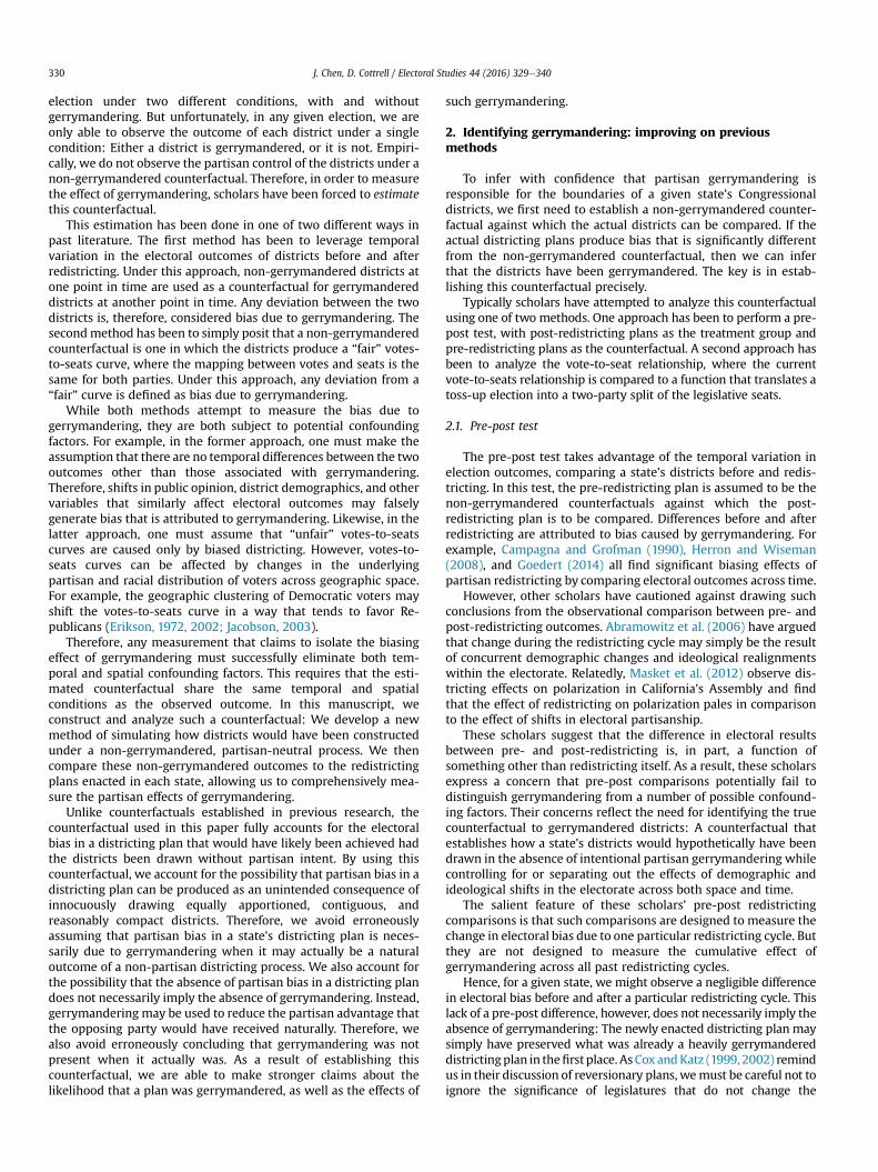
seat) more Republican than the median simulation in the state,whereas, in California, the enacted plan is about 4% (or just over 2seats) less Republican than the median simulation in the state. Inboth cases, the actual expected share of the seats won by Re-publicans is well outside the distribution of expected seat sharespredicted by the simulations. As a result, we can confidently claimthat the actual districting plan was not generated by the non-partisan districting procedure used in the simulations. Rather,assuming that the districts are drawn to be reasonably compact,contiguous, and equally apportioned (as they are in the simula-tions), the best explanation for the partisan difference in expectedseat share is that the districts were designed in a way that inten-tionally advantages one party over the other. In other words, thepartisan difference can be explained by gerrymandering.

In addition to Wisconsin and California, there is noticeablevariation across the states in the direction and degree to which theactual plans differ from the simulations. A partial explanation forthis variation is that it depends on the partisan control of the dis-tricting process. Under this explanation, we should be more likelyto observe districting plans that are designed to benefit a particularparty when that party is unobstructed in implementing the plan oftheir choice. For example, in states where the legislature isresponsible for approving district boundaries, we would expect tosee a map that favors a particular party when that party controlsboth chambers of the legislature as opposed to when it does not.

As a quick test to seewhether this explanation corresponds withour measure of gerrymandering, we divide the states according towho had decisive control over the redistricting process for the2011e12 congressional redistricting cycle. To make this determi-nation, we follow Justin Levitt’s survey of redistricting institutions,in which he identifies the party - if any - that was in control of theredistricting process for each of the states.4 Then, in Fig. 4, we plotthe difference in Republican seat share between the enacted dis-tricts and the simulated districts according to whether Republicansor Democrats control the districting process.

In addition, we single out pre-clearance states. Pre-clearancestates are required by Section 5 of the Voting Rights Act (VRA) toseek approval from the Department of Justice for any modificationsto their election laws.5 Under the VRA, the Department of Justice isresponsible for protecting minority representation in these statesby blocking any proposal that might have the effect of dilutingminority votes. Hence, congressional districts in these states areintentionally designed to avoid splitting blocs of minority voters ina way that might reduce their representation. As a result, thereexists a number of majority-minority districts that might not haveexisted otherwise had the districts been drawn at random.

Because of this, the resulting partisanship of the actual districtsin these states will likely deviate from the partisanship of oursimulated districts. Since minority groups protected under the VRAtend to vote overwhelmingly Democratic, districts produced byracial gerrymandering will likely be as distinct from our simula-tions as those produced by partisan gerrymandering. Therefore, inthese pre-clearance states, our measure of partisangerrymandering may actually be capturing the partisan effect ofracial gerrymandering instead.

Fig. 4 displays all four categories: states where Republicanscontrol the districting process, states where Democrats control thedistricting process, states with split partisan control of the dis-tricting process, and states that are required to obtain pre-clearance

4 Justin Levitt’s coding can be found at http://redistricting.lls.edu/who-partyfed.php.

5 These are states subject to pre-clearance prior to the ruling in Shelby County v.Holder, 133 S. Ct. 2612 (2013).

under the VRA.6 As we might expect, the difference between theactual and simulated Republican seat share corresponds with thesecategories. For example, among partisan controlled states, the di-rection of this difference can be partly explained by which party isin control of the districting process. The difference favors Re-publicans in 10 of the 12 states where Republicans have control andthe difference favors Democrats 4 of the 6 states where Democratshave control. However, the average effect is much stronger forRepublicans than it is for Democrats. This result suggests thatalthough both parties may use control over the districting processto their advantage, Republicans produce greater gains thanDemocrats.

Interestingly, however, there is evidence that Democrats areable to reclaim some of this Republican advantage through therace-conscious districting that occurs in pre-clearance states.Democrats do not control a single pre-clearance state and, there-fore, we would not expect Democrats to gain an advantage throughpartisan gerrymandering here. Yet, five of the eight states aresignificantly more Democratic than theywould have been had theirdistricts been drawn without respect to race or partisanship. EvenLouisiana, Alabama and Georgia, where districting was completelycontrolled by Republicans in the 2011e2012 cycle, produced dis-tricting plans that were more Democratic than the non-gerrymandered counterfactual plans. Racial consideration in thedistricting process, such as maintaining minority-majority districts,seems to produce stronger Democratic delegations in these statesthan they might otherwise produce without such considerations.The result suggests that the standards imposed by the Voting RightsAct may actually have the effect of not only improving minorityrepresentation but Democratic representation as well.

6. Total additional partisan seats due to gerrymandering

In our state-by-state analysis, we can see that both Republicansand Democrats make partisan gains through gerrymandering. Yet,what is the aggregate partisan effect of this gerrymandering onCongress as a whole? Running 200 simulated elections across thecongressional districts of every state, we calculate the expectedtotal number of Republicans that are elected for each simulation.Every simulated total can then be compared to the number of Re-publicans that the actual congressional boundaries of the 113thCongress are predicted to produce. Fig. 5 displays the results for 430congressional districts (we exclude Oregon’s 5 districts due to thelack of precinct-level data in the state).

Under the actual enacted plans, Republicans and Democrats arepredicted to nearly split the House. Republicans take 217.3 of the430 seats in expectation. Although this is a larger Republicandelegation than 91% of the simulations, it is only slightly larger indegree. In fact, the actual expected Republican seat share is withinthe range of the 95% confidence intervals as indicated by the greyvertical lines. The simulated counterfactual produces an average of216.4 Republican seats, which is approximately one fewer

Democratic party (Cain, 2012; Pierce and Larson, 2011). And because a Republican(Former New Jersey Attorney General, John Farmer, Jr.) was appointed to be the tie-breaking vote for New Jersey’s independent commission, we have coded the state’sdistricting process as being controlled by Republicans. These states are indicated byan asterisk in Fig. 4.

7 Shapefiles of precinct-level McCain-Obama votes were collected from theHarvard Election Data Archive available at http://projects.iq.harvard.edu/eda/data.

Fig. 4. Gerrymandering and political control over districting.

Fig. 5. The effect of gerrymandering on the total number of Republican seats in Congress.

J. Chen, D. Cottrell / Electoral Studies 44 (2016) 329e340 337

Fig. 6. The legislative consequences of gerrymandering by state.

J. Chen, D. Cottrell / Electoral Studies 44 (2016) 329e340338

Republican seat than the enacted plan is predicted to produce. Thissuggests that if districts were drawn randomly with respect topartisanship and race, Republicans would only expect to lose asingle seat in Congress to the Democrats. Therefore, although weidentify the partisan gains from gerrymandering in a number ofstates, these gains tend to be small and generally cancel out in theaggregate.

Such a result is meaningful because it contradicts a commonperception that major partisan gains in seat share are made in theHouse of Representatives through gerrymandering. Instead, theevidence suggests that the partisan makeup of the House would bealmost no different if gerrymandering - both partisan and racial -were altogether eliminated. Although some state delegationswould see significant change, the aggregate advantage received bya particular party in Congress would be almost zero.

Fig. 6 disaggregates the effect of gerrymandering by state. It

displays the magnitude of the expected partisan seat gain (or seatloss) that is due to gerrymandering in each state. It is calculated asthe difference between the expected Republican seat share of theactual districting plans and the median Republican seat shareacross the state’s 200 simulations. First, we can see that the state-level effect is limited. For any given state other than California,gerrymandering causes no more than one seat to switch parties. Inmost of these individual states, the partisan effect ofgerrymandering is negligible.

The greatest seat gain for Republicans occurs in states wherepartisans control the districting process. In fact, eight of the ninelargest gains for Republicans were in states where Republicanswere in control. On the other hand, most of the seat gain forDemocrats occurs either in California or pre-clearance states. Cal-ifornia contributes as many seats to the Democrats throughgerrymandering as the top three Republican gerrymanders

Fig. 7. The distibution of the likelihood of a Republican victory across Congressional districts: Simulated districts vs actual districts.

J. Chen, D. Cottrell / Electoral Studies 44 (2016) 329e340 339

combined. Democrat-controlled Maryland and Illinois are alsoamong the additional ten largest gains for Democrats. Yet,remarkably, six of the eight others are pre-clearance states. The pre-clearance states act to bolster Democratic representation, swappingRepublican seats for Democrats. Without these pre-clearancestates, Republicans would experience a slightly larger bias inaggregate seat share in Congress. We can aggregate the totalnumber of seats gained by gerrymandering across the four regimetypes mentioned in the previous section. This gives us a sense ofhow the regimes contibute to the net effect of gerrymandering inCongress. We find that among states controlled by Republicans,about five Republican seats are gained through gerrymandering.And among states controlled by Democrats, about three Republicanseats are lost by Gerrymandering. Moreover, Democrats gain about1.75 seats from states subject to preclearance. This suggests that theRepublican seat gain from Republican controlled states is coun-terbalanced by the seat loss in Democratic controlled and pre-clearance states.

We can get a clearer picture of the how the full set of simulatedelectoral outcomes differ from the actual outcomes by comparingthe distributions. Fig. 7 plots each of the 200 simulated densities ofthe 423 congressional districts belonging to the 42 multimemberstates (minus Oregon) onwhich we ran the simulations against thedensity of the actual congressional districts among those states. It isimmediately clear from the distribution of the actual districts thatthe most liberal districts tend to be outliers. In other words, there isa noticeable bump toward the left of the distribution reflecting thecollection of the most liberal districts that overwhelmingly supportDemocrats.

These districts are usually districts with large metropolitanareas where Democrats tend to concentrate. These packed liberaldistricts waste Democratic votes and thus allow Republicans toefficiently win a larger number of moderate districts by relativelysmall margins.Where the simulated distributions tend to have highnumbers of marginally Democratic districts relative to the numbersof marginally Republican districts, the actual distribution has highnumbers of marginally Republican districts relative to the numbersof marginally Democratic districts. Therefore, liberal districts aregetting far more Democrats than they should be getting under arandom draw. They are grossly overrepresented in a few districtswhile the remaining districts get a thin supply of the residual Re-publicans. This is enough to swing marginal Democratic districts in

the favor of Republicans. The effect of gerrymandering, therefore, isclear: Democrats gain safety in some of their most liberal districts,which, in effect, reduce their chances of winning more marginaldistricts. The Democrats lose seats in Congress as a result.

7. Conclusion

We have argued that there is a need to better identify when astate engages in gerrymandering, so as to not confuse partisangerrymandering with the type of partisan bias that results as anunintended consequence of drawing districts around ageographically-concentrated, partisan population. To avoid suchconfusion, we need to establish a baseline for what a state’s dis-tricts would look like if they had not been intentionally gerry-mandered. Using such a baseline, we could then compare the actualelectoral districting plans to a non-gerrymandered hypothetical. Ifthe plans differ significantly from the baseline, then it is likely thatthe actual plans were gerrymandered.

In this paper, we have established such a baseline. We usecomputer simulated districting plans that mimic the districtingdecisions performed by the states. The simulations draw compact,contiguous and equally apportioned districts around the uniquegeographic distribution of partisans in each state. The only differ-ence between the simulated and actual districts is that the simu-lated districts are not subject to intentional partisan or racialgerrymandering. Thus, any difference between the computer-produced plans and the actual plans should reliably be due togerrymandering.

By comparing the enacted post-2012 congressional districtingplans to their simulated counterfactual, we are able to more pre-cisely identify the effect of gerrymandering on partisan seat sharefor each state’s congressional delegation. While we find thatgerrymandering does play a role in altering electoral outcomesacross the states, in most states gerrymandering has little to noeffect on the partisan outcome of congressional elections. Instead,most of the outcomes can easily be explained by an unbiased dis-tricting procedure, where gerrymandering has been completelyremoved from the districting process.

Moreover, we find that in states where gerrymandering doeshave a significant effect on congressional elections, the effect isrelatively small. For example, other than in California, the partisangain from gerrymandering amounts to no more than a fraction of a

J. Chen, D. Cottrell / Electoral Studies 44 (2016) 329e340340

seat in any given state. While the total number of seats gained byRepublicans is greater than the total number of seats gained byDemocrats, the net effect of gerrymandering in Congress is onlymarginal. In fact, we find that Republicans are expected to net nomore than one additional seat as result of it.

However, the type of gerrymandering that benefits Republicansappears to be different from the type of gerrymandering thatbenefits Democrats. For example. Republicans appear tomakemostof their gains as a result of having full institutional control over thedistricting procedures in their states. This allows them to etchpartisan bias into their districts without any effective opposition.Our analysis reveals that Republicans tend to take advantage ofthese opportunities.

On the other hand, because there are fewer states whereDemocrats have institutional control over the districting process,Democrats gain fewer seats from partisan gerrymandering thanRepublicans. In fact, counterintuitively, we observe that much ofthe significant state-level bias toward Democrats occurs in stateswhere Republicans hold legislative majorities. It turns out thatthese states are also pre-clearance states that engage in racialgerrymandering to meet the standards set out by the Voting RightsAct. Therefore, Democrats tend to gain seats as a result of racial biasinstead of partisan bias.

If we were to remove the pre-clearance states from the analysis,then we would observe that gerrymandering tends to favor Re-publicans. However, the additional seats that Republicans wouldgain on average from gerrymandering - evenwithout pre-clearancestates - is marginal. It is simply the case that the effect ofgerrymandering is small and that removing bias from districtingprocess - whether it is racial or partisan - is not likely to change thepartisan composition of Congress.

References

Abramowitz, Alan I., 1983. Partisan redistricting and the 1982 congressional elec-tions. J. Polit. 45 (03), 767e770.

Abramowitz, Alan I., Alexander, Brad, Gunning, Matthew, 2006. Incumbency,redistricting, and the decline of competition in US House elections. J. Polit. 68(1), 75e88.

Ansolabehere, Stephen, Rodden, Jonathan, Snyder, James M., 2006. Purple America.J. Econ. Perspect. 20 (2), 97e118.

Cain, Bruce E., 2012. Essay and feature: redistricting commissions: a better politicalbuffer? Yale LJ 121, 1808e2405.

Campagna, Janet, Grofman, Bernard, 1990. Party control and partisan bias in 1980scongressional redistricting. J. Polit. 52 (04), 1242e1157.

Chen, Jowei, Rodden, Jonathan, 2013. Unintentional gerrymandering: political ge-ography and electoral bias in legislatures. Q. J. Political Sci. 8 (3), 239e269.

Cox, Gary W., Katz, Jonathan N., 1999. The reapportionment revolution and bias inUS congressional elections. Am. J. Political Sci. 812e841.

Cox, Gary W., Katz, Jonathan N., 2002. Elbridge Gerry’s Salamander: The ElectoralConsequences of the Reapportionment Revolution. Cambridge University Press.

Erikson, Robert S., 1972. Malapportionment, gerrymandering, and party fortunes incongressional elections. Am. Political Sci. Rev. 1234e1245.

Erikson, Robert S., 2002. Sources of partisan bias in US congressional elections: anupdate stimulated by Ron Johnston’s essay. Polit. Geogr. 21 (1), 49e54.

Ferejohn, John A., 1977. On the decline of competition in congressional elections.Am. Political Sci. Rev. 166e176.

Gelman, Andrew, King, Gary, 1994. Enhancing democracy through legislativeredistricting. Am. Political Sci. Rev. 88 (03), 541e559.

Glazer, Amihai, Grofman, Bernard, Robbins, Marc, 1987. Partisan and incumbencyeffects of 1970s congressional redistricting. Am. J. Political Sci. 680e707.

Goedert, Nicholas, 2014. Gerrymandering or geography? How Democrats won thepopular vote but lost the Congress in 2012. Res. Polit. 1 (1), 2053168014528683.

Herron, Michael C., Wiseman, Alan E., 2008. Gerrymanders and theories of lawmaking: a study of legislative redistricting in Illinois. J. Polit. 70 (01), 151e167.

Jacobson, Gary C., 2003. Terror, terrain, and turnout: explaining the 2002 midtermelections. Political Sci. Q. 118 (1), 1e22.

Kendall, Maurice G., Stuart, Alan, 1950. The law of the cubic proportion in electionresults. Br. J. Sociol. 1 (3), 183e196.

King, Gary, 1989. Representation through legislative redistricting: a stochasticmodel. Am. J. Political Sci. 787e824.

Masket, Seth E., Winburn, Jonathan, Wright, Gerald C., 2012. The gerrymanderersare coming! Legislative redistricting won’t affect competition or polarizationmuch, no matter who does it. PS Political Sci. Polit. 45 (01), 39e43.

McDonald, Michael P., 2004. A comparative analysis of redistricting institutions inthe United States, 2001e02. State Polit. Policy Q. 4 (4), 371e395.

McDonald, Michael, 2009. Seats to Votes Ratios in the United States (UnpublishedPaper).

Openshaw, Stan, 1984. The Modifiable Areal Unit Problem. Geobooks, Norwich,England.

Pierce, Olga, Larson, Jeff, 2011. How Democrats Fooled California’s RedistrictingCommission. http://www.propublica.org/article/how-democrats-fooled-californias-redistricting-commission.

Squire, Peverill, 1985. Results of partisan redistricting in seven US states during the1970s. Legis. Stud. Q. 259e266.

Tufte, Edward R., 1973. The relationship between seats and votes in two-partysystems. Am. Political Sci. Rev. 540e554.