Electric Fields in LVDC cables

D. Antoniou, A. Tzimas and S. M. Rowland The University of Manchester

School of Electrical and Electronic Engineering

M13 9PL, UK

Abstract – The operation of legacy LVAC distribution cables

under DC is considered in this work. The electric field

distribution in cable insulation under DC voltage is governed by

the electrical conductivity of the material unlike the AC case

where it is dependent on the permittivity of the materials.

Temperature, water ingress and chemical ageing can increase the

conductivity of the insulation. A good insulator should exhibit the

least conductivity possible in order to minimise the current

flowing through the material. Variations in insulation properties

leading to reduced uniformity could cause local elevated stresses

in the insulating material which could lead to cable failure. This

paper shows how the electric field distribution in typical LVAC

cables changes as the conductivity of the insulation is altered due

to changes in temperature and electric field when operated under

DC. A 4-core Paper Insulated Lead Covered (PILC) belted cable

is simulated in COMSOL Multiphysics both under AC and DC

conditions and the results are compared.

I. INTRODUCTION

This work is part of the ‘Top and Tail Project’, a

collaborative project funded by the EPSRC Grand Challenge

Programme. The project is focused on the physical

infrastructure change in energy networks required to move the

UK to a low carbon economy necessary to achieve the

Government’s target of reducing CO2 emissions by 2050. The

project is divided in to two parts, the ‘Top’ and the ‘Tail’, and

intended to be high risk and long-term in nature. The ‘Top’

focuses on the Transmission part of the network whereas the

‘Tail’ focuses on the last mile of the Distribution network. This

work reported here is part of the ‘Tail’.

The purpose of this work is to consider the feasibility of

operating existing LVAC underground cables under DC. Using

the existing infrastructure is potentially more economical and

less time consuming than relaying new cables in urban

environments. Studies have shown that the use of DC in the

distribution network can substantially increase the power

transfer in the network [1]. This assumes that the cables will

operate as reliably under DC as they do under AC.

The power capacity of the present LVAC distribution

network is limited by the voltage of the system. Increasing the

current is not the best solution since there will be an increase in

the heat produced thus increasing the losses in the system. The

insulation in an AC cable is rated at the peak operating voltage.

In a typical 230 Vrms AC system the peak voltage is 325 Vpeak.

A question is raised from this: “Could the system be reliable at

325 VDC?”. Extensive research has been carried out on HVAC

and HVDC cables and the breakdown mechanisms are

relatively well known. LVAC cables do not exhibit the

breakdown phenomena present under high voltages and they

are known to be very reliable. As a result little research has

been carried out. A key difference between the AC and DC

cases is that the electric field distribution under AC depends on

the permittivities of the dielectrics whereas under DC it

depends on the conductivity of the materials [2]. As a result,

water ingress presents different issues in AC and DC cables

since water changes both the permittivity and the conductivity.

Conductivity is also more affected by changes in temperature

and the local electric field in the insulation and so must also be

considered for DC cables.

The most common paper insulated cable used in the UK

distribution network is the 4-core PILC BS6480 cable [3]. The

cable is rated at 600/1000 V (phase to ground/ phase to phase).

FEM simulations using COMSOL are used in this work to

analyse how the electric field behaves in the cable under DC.

The Joule heating module is used to calculate the heat

generated due to the resistance of the cable. The Electric circuit

module is coupled with the Joule heating model to provide a

means of changing the load for each core in the cable. Electric

field stress distribution is compared for both AC and DC under

normal conditions as well as in the presence of a gas filled

voids and moisture.

II. MODELLING OF THE CABLE

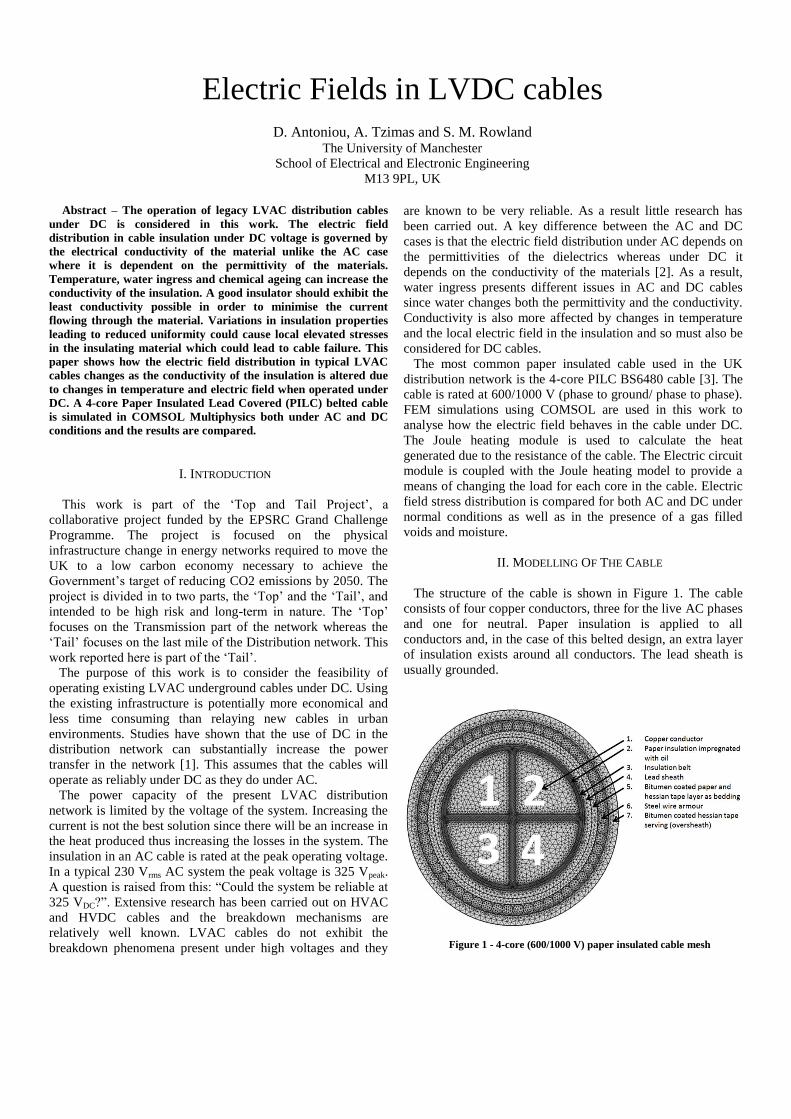
The structure of the cable is shown in Figure 1. The cable

consists of four copper conductors, three for the live AC phases

and one for neutral. Paper insulation is applied to all

conductors and, in the case of this belted design, an extra layer

of insulation exists around all conductors. The lead sheath is

usually grounded.

Figure 1 - 4-core (600/1000 V) paper insulated cable mesh

1 2 3 4

Covering the lead sheath there is a layer of either a steel wire

or tape armour used to provide stiffness and protection to the

cable. The last layer of the cable is the oversheath (jacket)

which is usually made of PVC or bitumen. The neutral is

separated from the earth which usually is connected to the

sheath and armour wires.

In this model the effect of strand geometry is not included,

and the field is discussed in areas of greatest geometrical

uniformity in the insulation so that the impact of dielectric

properties can be easily considered. Careful planning was

carried out to determine the minimum number of elements

required to obtain sufficiently accurate results and 80,000

elements were used for meshing the initial model. After the

introduction of a void into the model insulation material,

manual meshing was used to eliminate rough edges on

interfaces which could falsely suggest an enhanced local field.

Roughly 100,000 elements were used for the void model and

around 160,000 where used for the introduction of moisture.

Table 1 show the material properties used in the simulation and

Table 2 the domain parameters.

The copper conductors in the cable are stranded but for

simplification the electrical conductivity of copper was reduced

to compensate for the packing factor. Convective cooling was

applied on the outermost surface of the cable. Depending on

the study, different voltage levels were applied on the four

conductors. The lead sheath was always kept at ground

potential. Similarly temperature conditions were altered

depending on the study and are discussed further on.

Table 1 - Material properties used in the simulation

Copper Steel PVC Paper insulation

Lead Air Water

Electrical Cond. (S/m)

6.0x107 4.0x106 1.0x10-15 1.0x10-16 4.6x106 5.0x10-15 5.5x10-4

Thermal Cond. (W/(m*K))

400 44.5 0.10 0.11 35 0.025 0.60

Heat Capacity (J/(kg*K))

385 475 2300 1200 130 1012 4181

Relative permittivity (εr)

1.0 1.0 8.0 3.6 1.0 1.0 80

Density (kg/m3)

8700 7850 1760 1200 11340 1.184 1000

Initial Temp. (oC)

25 25 25 25 25 25 25

Heat transfer coefficient (W/m2*K)

7

Table 2 - Domain parameters

III. DC CONDUCTIVITY

The electrical conductivity depends on the temperature and the

electric field in the insulation [4]. Equation 1 is an empirical

formula relating the conductivity to temperature and electric

field where ko is the specific electrical conductivity at 0oC and

zero field, T is the temperature difference from 0°C (T1-273) in

K, T1 is the local insulation temperature in K, E is the electric

field in kV/mm, a is the temperature coefficient of conductivity

and β is the electric field strength coefficient of conductivity.

( | |) ( ) ( | |) (1)

This formula was entered as a conductivity expression in the

FEA tool. Values from the literature of α and β were assumed

to be 0.1 and 0.03 respectively [5].

IV. ELECTRIC FIELD DISTRIBUTION IN THE CABLES

Other parameters that can affect the electric field distribution

are the geometry of the cable and/or any imperfections present

in the insulation. Given a uniform conductivity, the highest

electric field should be close to the conductor rather than the

sheath. In this study the model was coupled to circuit physics.

This module allowed simulation of the current flowing through

each conductor which was fed back to the Joule Heating

module. Conductors 1, 2 and 4 were run at 265 A each. The

maximum temperature observed was 57.4 oC at the cores. The

sheath temperature was 54 oC creating a temperature gradient

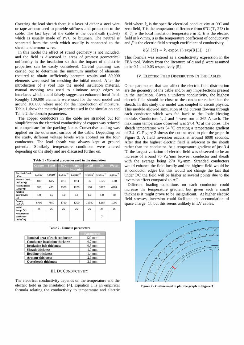
of 3.4 oC. Figure 2 shows the cutline used to plot the graph in

Figure 3. A field inversion occurs at around 6000 seconds.

After that the highest electric field is adjacent to the sheath

rather than the conductor. At a temperature gradient of just 3.4 oC the largest variation of electric field was observed to be an

increase of around 75 Vdc/mm between conductor and sheath

with the average being 270 Vdc/mm. Stranded conductors

would enhance the field locally and the highest field would be

at conductor edges but this would not change the fact that

under DC the field will be higher at several points due to the

inversion effect compared to AC.

Different loading conditions on each conductor could

increase the temperature gradient but given such a small

thickness it might prove to be insignificant. At higher electric

field stresses, inversion could facilitate the accumulation of

space charge [1], but this seems unlikely in LV cables.

Figure 2 - Cutline used to plot the graph in Figure 3

Parameters

Nominal area of each conductor 120 mm2

Conductor insulation thickness 0.7 mm

Insulation belt thickness 0.5 mm

Sheath thickness 1.7 mm

Bedding thickness 1.4 mm

Armour thickness 2.5 mm

Oversheath thickness 2.3 mm

Figure 3 - Electric field across the insulation, as a function of time.

Colour lines are at different times (seconds).

V. TEMPERATURE EFFECTS

Field inversion can be increased by increasing the

temperature differences in the cable. To better demonstrate the

effect, temperature boundary conditions were set on the

conductors and sheath. The temperature difference was raised

to 7.4 oC. Two studies were run, one DC and the other AC. In

the DC study, conductors 1 and 2 were set at 325 V, and

conductors 3 and 4 earthed. In the AC study, conductors 1, 2,

and 4 were three phase at 230 Vrms, and conductor 3 earthed.

The simplest geometrical cutline, shown in Figure 2, is used to

illustrate results so only the phase to ground electric field is

considered in this study. Figure 4 shows the results from the

DC study. A variation of around 0.16 kV/mm between

conductor and sheath is observed. The average is still at 0.27

kV/mm since the voltage and insulation thickness have not

changed.

Figure 5 shows the results of the AC study. These cycles

were taken after a sufficient time in order to reach temperature

equilibrium. Six points on the first half crest of the waveforms

are plotted ranging from 0 V to a peak of 325 V.

Figure 4 - Electric field under DC with a 7.4 oC gradient

Figure 5 - Electric field under AC with a 7.4 oC gradient, within an AC

quarter cycle. Coloured lines are at different times (seconds).

The graph shows the maximum electric field at 0.28 kV/mm

at the conductor side due to geometry. What should be noticed

is that under AC the electric field never reaches the maximum

electric field seen under DC. Under DC there is a constant high

electric field near the sheath whereas under AC is more

uniform. The insulation under DC would be subjected to a

continuously high field (polarity reversals being unlikely in the

distribution network) whereas under AC it will continually

reverse polarity. At these low voltages this might prove to be

insignificant but in an aged cable, temperature variations could

be great further enhancing the effect.

VI. EFFECTS OF IMPERFECTIONS

Imperfections in the insulation such as voids may cause the

insulation to breakdown. In HV cables partial discharge is

mainly responsible for this phenomenon [6]. The voids are gas

filled thus having a lower dielectric constant. This causes a

higher electric field inside the void. Air has a lower dielectric

strength than the insulation therefore a partial breakdown

occurs in the void. An elliptical void was introduced in the

model with: an x-radius of 100 µm, a y-radius of 50 µm and a

z-radius of 50 µm. Void geometry can greatly impact the local

electric field. Studies on how different geometries enhance the

field are well established [7]. This study concentrates on the

enhancement due to different currents rather than different

geometries.

Figure 6 - Position and size of the void

0.4

0.35

0.3

0.25

0.2

0.15

0.1

0.05

0

0.4

0.35

0.3

0.25

0.2

0.15

0.1

0.05

0

0.305

0.3

0.295

0.29

0.285

0.28

0.275

0.27

0.265

0.26

0.255

0.25

0.245

0.24

0.235

Electric Field (kV/mm) Electric Field

(kV/mm)

Electric Field (kV/mm)

0 0.1 0.2 0.3 0.4 0.5 0.6 0.7 0.8 0.9 1.0 1.1 1.2 Arc length (mm)

0 0.1 0.2 0.3 0.4 0.5 0.6 0.7 0.8 0.9 1.0 1.1 1.2 Arc length (mm)

0 0.1 0.2 0.3 0.4 0.5 0.6 0.7 0.8 0.9 1.0 1.1 1.2 Arc length (mm)

0 500 1000 1500 2000 2500 3000 3500 4000 6500 9000 12000

1200 1200.001 1200.002 1200.003 1200.004 1200.005

1200

Figure 7 - Electric field enhancement as a result of the void.

Figure 6 shows the void in the cable insulation belt and a new

cutline is shown. In Figure 7 the graph compares the field

enhancement in AC and DC cases and again the enhancement

is greater under DC. Placing the void between two conductors

will give results according to the voltage levels. This will not

however change the fact that conductivity changes with

temperature, and as a result, changes the electric field

distribution under DC. The of the fields in the DC case may be

larger, but the fields are still well less than 1 kV/mm, and these

voltages are not enough to cause discharges in such voids.

Paschen’s law indicates that conventional models of partial

discharge associated with high voltage insulation will not occur

at voltages lower than 350 V which is above the maximum

voltage to be seen in a void in this system configuration.

VII. MOISTURE EFFECTS

Moisture was introduced into the model. Figure 8 shows the

arrangement of the water content and the field distribution. In

reality, the volume, spatial distribution and properties of the

water will greatly vary from one cable to the other. The field

enhancement is higher than previous cases considered. The

voltage potential distribution is not uniform between conductor and sheath anymore and the electric field increases. This, along

with the change in geometry, causes a higher local electric

field. Under DC the electric field is still higher than under AC.

Figure 8 - Electric field distribution with water present

The field created by the water ingress is still not high, but it

may be significant in that it may drive moisture diffusion, and

the divergence it introduces may drive dielectrophoresis.

Because the cable insulation is not uniform physically more

work is required to understand moisture diffusion [8, 9].

VIII. CONCLUSIONS

The simulation of the 4-core PILC cable has shown that the

electric field distribution under DC is essentially different to

that in the AC case. A field inversion occurs which could

facilitate space charge accumulation but at these low voltages

and low electric field stresses it is unlikely to be of great

importance. Under AC, the effect of temperature variation

between the conductor and sheath has no impact on the

distribution of the electric field. Energising with DC results in

a higher electric field towards the sheath, and so the insulation

will not be uniformly stressed as in the AC case.

The presence of imperfections further cause enhancement in

localised fields and will be higher under DC. Nonetheless the

low voltages of a few hundred volts are insufficient to allow

partial discharge by the classical models associated with high

voltage cables. In the presence of water, DC will produce a

greater electric field enhancement compared to AC. A key

issue is whether such fields can drive moisture migration.

Equally importantly when considering an existing network will

be to consider the behaviour of existing joints in networks [10].

ACKNOWLEDGMENTS

The authors gratefully acknowledge the RCUK's Energy

Programme for the financial support of this work through the

Top & Tail Transformation programme grant, EP/I031707/1

(http://www.topandtail.org.uk/).

REFERENCES

[1] Tzimas, A.; Antoniou, D.; Rowland, S.M., ‘Low voltage DC cable insulation challenges and opportunities’ Conference on Electrical

Insulation and Dielectric Phenomena, pp. 696-699, 2012

[2] Morshuis P.H.F., Roefs R.J., Snitt J.J., Contin A., Montinari G.C., ‘The stability of mass-impregnated paper AC cables operated at DC voltage’

Proc. JiCable, 1999

[3] British Standard BS6480, 1988 [4] Shanshan Qin and Boggs, S., ‘Design considerations for high voltage DC

components’ Electrical Insulation Magazine, IEEE, vol.28, no.6, pp.36-44,

Nov.-Dec. 2012 [5] Electric Cables Handbook – BICC Cables, third Edit., pp. 575-576, 1997

[6] Dissado, L. A., and Fothergill, J. C., ‘Electrical Degradation and

Breakdown in Polymers’ Peter Peregrinus for IEE: London, 1992 [7] Blackburn, H. N. O; T. R., Phung, B., Zhang, T. H., Khawaja, R. H.,

"Investigation of Electric Field Distribution in Power Cables with

Voids," Int Conf. on Properties and Applications of Dielectric Materials,

637-640, 2006

[8] Rowland, S. M., and Wang, M., ‘Fault Development in Wet, Low Voltage,

Oil-Impregnated Paper Insulated Cables’ IEEE Trans DEI 15 Issue 2, 484-491 2008

[9] Wang, M., Rowland, S. M., and Clements, P. E., ‘Moisture Ingress into

Low Voltage Oil-Impregnated-Paper Insulated Distribution Cables’ IET Proc Sci., Meas. & Tech. 1 Issue 5, 276-283, 2007

[10] Antoniou, D., Tzimas, A., Rowland, S. M., ‘DC utilization of existing

LVAC distribution cables’ Electrical Insulation Conference, 2013

0 0.1 0.2 0.3 0.4 0.5 0.6 0.7 0.8 0.9 1.0 1.1 1.2

Max=3.92 kV/mm Max=4.98 kV/mm