electric power transmission system engineering analysis and design_t. gonen.pdf

Scilab Textbook Companion forElectric Power Transmission SystemEngineering Analysis And Design

by T. Gonen1

Created byKavan A. B

B.EElectrical Engineering

Sri Jayachamarajendra College Of EngineeringCollege Teacher

R. S. Ananda MurthyCross-Checked byK. V. P. Pradeep

June 12, 2014

1Funded by a grant from the National Mission on Education through ICT,http://spoken-tutorial.org/NMEICT-Intro. This Textbook Companion and Scilabcodes written in it can be downloaded from the ”Textbook Companion Project”section at the website http://scilab.in

Book Description

Title: Electric Power Transmission System Engineering Analysis And De-sign

Author: T. Gonen

Publisher: Crc Press, Florida

Edition: 2

Year: 2009

ISBN: 9781439802540

1

Scilab numbering policy used in this document and the relation to theabove book.

Exa Example (Solved example)

Eqn Equation (Particular equation of the above book)

AP Appendix to Example(Scilab Code that is an Appednix to a particularExample of the above book)

For example, Exa 3.51 means solved example 3.51 of this book. Sec 2.3 meansa scilab code whose theory is explained in Section 2.3 of the book.

2

Contents

List of Scilab Codes 4

2 TRANSMISSION LINE STRUCTURES AND EQUIPMENT 7

3 FUNDAMENTAL CONCEPTS 10

4 OVERHEAD POWER TRANSMISSION 15

5 UNDERGROUND POWER TRANSMISSION AND GASINSULATED TRANSMISSION LINES 48

6 DIRECT CURRENT POWER TRANSMISSION 76

7 TRANSIENT OVERVOLTAGES AND INSULATION CO-ORDINATION 90

8 LIMITING FACTORS FOR EXTRA HIGH AND ULTRA-HIGH VOLTAGE TRANSMISSION 103

9 SYMMETRICAL COMPONENTS AND FAULT ANALY-SIS 107

10 PROTECTIVE EQUIPMENT AND TRANSMISSION SYS-TEM PROTECTION 137

12 CONSTRUCTION OF OVERHEAD LINES 149

13 SAG AND TENSION ANALYSIS 157

14 APPENDIX C REVIEW OF BASICS 161

3

List of Scilab Codes

Exa 2.1 calculate tolerable touch step potential . . . . . . . . . 7Exa 3.1 determine SIL of the line . . . . . . . . . . . . . . . . 10Exa 3.2 determine effective SIL . . . . . . . . . . . . . . . . . 11Exa 3.3 calculate RatedCurrent MVARrating CurrentValue . . 13Exa 4.1 calculate LinetoNeutralVoltage LinetoLineVoltage Load-

Angle . . . . . . . . . . . . . . . . . . . . . . . . . . . 15Exa 4.2 calculate percentage voltage regulation using equation 20Exa 4.3 mutual impedance between the feeders . . . . . . . . . 21Exa 4.4 calculate A B C D Vs I pf efficiency . . . . . . . . . . 22Exa 4.5 calculate A B C D Vs I pf efficiency using nominal pi . 24Exa 4.6 calculate A B C D Vs I pf P Ploss n VR Is Vr . . . . . 27Exa 4.7 find equivalent pi T circuit and Nominal pi T circuit . 31Exa 4.8 calculate attenuation phase change lamda v Vir Vrr Vr

Vis Vrs Vs . . . . . . . . . . . . . . . . . . . . . . . . 32Exa 4.9 calculate SIL . . . . . . . . . . . . . . . . . . . . . . . 35Exa 4.10 determine equ A B C D constant . . . . . . . . . . . . 36Exa 4.11 determine equ A B C D constant . . . . . . . . . . . . 37Exa 4.12 calculate Is Vs Zin P var . . . . . . . . . . . . . . . . 39Exa 4.13 calculate SIL Pmax Qc Vroc . . . . . . . . . . . . . . 41Exa 4.14 calculate SIL Pmax Qc cost Vroc . . . . . . . . . . . . 43Exa 4.15 calculate La XL Cn Xc . . . . . . . . . . . . . . . . . 45Exa 5.1 calculate Emax Emin r . . . . . . . . . . . . . . . . . 48Exa 5.2 calculate potential gradient E1 . . . . . . . . . . . . . 49Exa 5.3 calculate Ri Power loss . . . . . . . . . . . . . . . . . 51Exa 5.4 calculate charging current Ic . . . . . . . . . . . . . . 52Exa 5.5 calculate Ic Is pf . . . . . . . . . . . . . . . . . . . . . 53Exa 5.6 calculate Geometric factor G1 Ic . . . . . . . . . . . . 55Exa 5.7 calculate Emax C Ic Ri Plc Pdl Pdh . . . . . . . . . . 56

4

Exa 5.8 calculate Rdc Reff percent reduction . . . . . . . . . . 58Exa 5.9 calculate Xm Rs deltaR Ra ratio Ps . . . . . . . . . . 59Exa 5.10 calculate zero sequence impedance Z00 Z0 Z0a . . . . 62Exa 5.11 calculate C0 C1 C2 X0 X1 X2 I0 I1 I2 . . . . . . . . . 65Exa 5.12 calculate Zabc Z012 . . . . . . . . . . . . . . . . . . . 67Exa 5.15 calculate PlOH PlGIL ElOH ElGIL ClOH ElavgGIL

ClavgOH ClavgGIL Csavings breakeven period . . . . 69Exa 5.16 calculate A1 A2 A of OH GIL and submarine transmis-

sion line . . . . . . . . . . . . . . . . . . . . . . . . . . 72Exa 6.1 determine Vd Id ratio of dc to ac insulation level . . . 76Exa 6.2 determine Vd ratio of Pdc to Pac and Ploss dc to Ploss

ac . . . . . . . . . . . . . . . . . . . . . . . . . . . . . 78Exa 6.3 calculate KVA rating Wye side KV rating . . . . . . . 79Exa 6.4 determine Xc for all 3 possible values of ac system reac-

tance . . . . . . . . . . . . . . . . . . . . . . . . . . . 80Exa 6.5 calculate u Vdr pf Qr . . . . . . . . . . . . . . . . . . 82Exa 6.6 determine alpha u pf Qr . . . . . . . . . . . . . . . . . 84Exa 6.7 determine u mode Id or Vdr . . . . . . . . . . . . . . . 85Exa 6.10 determine Vd0 E u pf Qr No of bucks . . . . . . . . . 87Exa 7.1 determine surge Power surge current . . . . . . . . . . 90Exa 7.2 determine surge Power surge current . . . . . . . . . . 91Exa 7.4 determine Crv Cri vb v Crfv ib i Crfi . . . . . . . . . . 92Exa 7.5 determine if Cr Crf v i vb ib plot of voltage and current

surges . . . . . . . . . . . . . . . . . . . . . . . . . . . 94Exa 7.6 determine Crs Crr lattice diagram volatge plot of receiv-

ing end voltage with time . . . . . . . . . . . . . . . . 97Exa 8.1 determine disruptive critical rms V0 and visual critical

rms Vv . . . . . . . . . . . . . . . . . . . . . . . . . . 103Exa 8.2 determine total fair weather corona loss Pc . . . . . . 104Exa 9.1 determine symmetrical components for phase voltages 107Exa 9.2 determine complex power V012 I012 . . . . . . . . . . 109Exa 9.3 determine line impedance and sequence impedance ma-

trix . . . . . . . . . . . . . . . . . . . . . . . . . . . . 111Exa 9.4 determine line impedance and sequence impedance ma-

trix of transposed line . . . . . . . . . . . . . . . . . . 112Exa 9.5 determine mo m2 for zero negative sequence unbalance 114Exa 9.6 determine Pabc Cabc C012 d0 d2 . . . . . . . . . . . 116

5

Exa 9.9 determine Iphase Isequence Vphase Vsequence Lineto-LineVoltages at Faultpoints . . . . . . . . . . . . . . . 118

Exa 9.10 determine Isequence Iphase Vsequence at fault G1 G2 120Exa 9.11 determine Iphase Isequence Vphase Vsequence Lineto-

LineVoltages at Faultpoints . . . . . . . . . . . . . . . 124Exa 9.12 determine Iphase Isequence Vphase Vsequence Lineto-

LineVoltages at Faultpoints . . . . . . . . . . . . . . . 127Exa 9.13 determine Iphase Isequence Vphase Vsequence Lineto-

LineVoltages at Faultpoints . . . . . . . . . . . . . . . 129Exa 9.14 determine admittance matrix . . . . . . . . . . . . . . 131Exa 9.15 determine uncoupled positive and negative sequence . 133Exa 9.16 determine Xc0 C0 Ipc Xpc Lpc Spc Vpc . . . . . . . . 134Exa 10.1 calculate subtransient fault current in pu and ampere . 137Exa 10.2 determine max Idc Imax Imomentary Sinterrupting Smo-

mentary . . . . . . . . . . . . . . . . . . . . . . . . . . 138Exa 10.4 determine Rarc Z LineImpedanceAngle with Rarc and

without . . . . . . . . . . . . . . . . . . . . . . . . . . 140Exa 10.5 determine protection zones and plot of operating time

vs impedance . . . . . . . . . . . . . . . . . . . . . . . 141Exa 10.6 determine Imax CT VT ZLoad Zr . . . . . . . . . . . 144Exa 10.7 determine setting of zone1 zone2 zone3 of mho relay R12 147Exa 12.1 calculate cost of relocating affordability . . . . . . . . 149Exa 12.2 calculate pressure of wind on pole and conductors . . . 151Exa 12.3 calculate min required pole circumference at ground line 152Exa 12.4 calculate Th beta Tv Tg . . . . . . . . . . . . . . . . . 154Exa 13.1 calculate length sag Tmax Tmin Tappr . . . . . . . . 157Exa 13.2 calculate Wi Wt P We sag vertical sag . . . . . . . . . 158Exa 1.C determine power S12 P12 Q12 . . . . . . . . . . . . . 161Exa 2.C determine reactance Zbhv Zblv Xhv Xlv . . . . . . . 162Exa 3.C determine turns ratio Xlv Xpu . . . . . . . . . . . . . 164Exa 4.C determine KVA KV Zb Ib I new Zpu V1 V2 V4 S1 S2

S4 table . . . . . . . . . . . . . . . . . . . . . . . . . . 166Exa 5.C determine inductive reactance using equ C135 and tables 170Exa 6.C determine shunt capacitive reactance using equ C156

and tables . . . . . . . . . . . . . . . . . . . . . . . . . 172

6

Chapter 2

TRANSMISSION LINESTRUCTURES ANDEQUIPMENT

Scilab code Exa 2.1 calculate tolerable touch step potential

1 // ELECTRIC POWER TRANSMISSION SYSTEM ENGINEERINGANALYSIS AND DESIGN

2 // TURAN GONEN3 // CRC PRESS4 // SECOND EDITION56 // CHAPTER : 2 : TRANSMISSION LINE STRUCTURES AND

EQUIPMENT78 // EXAMPLE : 2 . 1 :9 clear ; clc ; close ; // C l ea r the work space and

c o n s o l e1011 // GIVEN DATA12 t_s = 0.49 ; // Human body i s i n c o n t a c t with 60 Hz

power f o r 0 . 4 9 s e c13 r = 100 ; // R e s i s t i v i t y o f s o i l based on IEEE s td

7

80−20001415 // CALCULATIONS16 // For c a s e ( a )17 v_touch50 = 0.116*(1000+1.5*r)/sqrt(t_s) ; //

Maximum a l l o w a b l e touch v o l t a g e f o r 50 kg bodywe ight i n v o l t s

1819 // For c a s e ( b )20 v_step50 = 0.116*(1000+6*r)/sqrt(t_s) ; // Maximum

a l l o w a b l e s t e p v o l t a g e f o r 50 kg body we ight i nv o l t s

21 // Above Equat ions o f c a s e ( a ) & ( b ) a p p l i c a b l e i fno p r o t e c t i v e s u r f a c e l a y e r i s used

2223 // For meta l to meta l c o n t a c t below e q u a t i o n h o l d s

good . Hence r e s i s t i v i t y i s z e r o24 r_1 = 0 ; // R e s i s t i v i t y i s z e r o2526 // For c a s e ( c )27 v_mm_touch50 = 0.116*(1000)/sqrt(t_s) ; // Maximum

a l l o w a b l e touch v o l t a g e f o r 50 kg body we ight i nv o l t s f o r meta l to meta l c o n t a c t

2829 // For c a s e ( d )30 v_mm_touch70 = 0.157*(1000)/sqrt(t_s) ; // Maximum

a l l o w a b l e touch v o l t a g e f o r 70 kg body we ight i nv o l t s f o r meta l to meta l c o n t a c t

3132 // DISPLAY RESULTS33 disp(”EXAMPLE : 2 . 1 : SOLUTION :−”) ;

34 printf(”\n ( a ) T o l e r a b l e Touch p o t e n t i a l , V touch50= %. f V , f o r 50 kg body we ight \n”,v_touch50) ;

35 printf(”\n ( b ) T o l e r a b l e Step p o t e n t i a l , V step50 =%. f V , f o r 50 kg body we ight \n”,v_step50) ;

36 printf(”\n ( c ) T o l e r a b l e Touch Vo l tage f o r metal−to−meta l c o n t a c t , V mm touch50 = %. 1 f V , f o r 50 kg

body we ight \n”,v_mm_touch50) ;

8

37 printf(”\n ( d ) T o l e r a b l e Touch Vo l tage f o r metal−to−meta l c o n t a c t , V mm touch70 = %. 1 f V , f o r 70 kg

body we ight \n”,v_mm_touch70) ;

9

Chapter 3

FUNDAMENTAL CONCEPTS

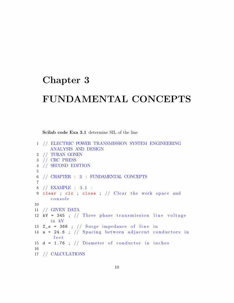
Scilab code Exa 3.1 determine SIL of the line


2 // TURAN GONEN3 // CRC PRESS4 // SECOND EDITION56 // CHAPTER : 3 : FUNDAMENTAL CONCEPTS78 // EXAMPLE : 3 . 1 :9 clear ; clc ; close ; // C l ea r the work space and

c o n s o l e1011 // GIVEN DATA12 kV = 345 ; // Three phase t r a n s m i s s i o n l i n e v o l t a g e

i n kV13 Z_s = 366 ; // Surge impedance o f l i n e i n14 a = 24.6 ; // Spac ing between a d j a c e n t c o n d u c t o r s i n

f e e t15 d = 1.76 ; // Diameter o f conduc to r i n i n c h e s1617 // CALCULATIONS

10

18 SIL = (kV)^2/Z_s ; // Surge Impedance l o a d i n g o fl i n e i n MW


22 printf(”\n Surge Impedance Loading o f l i n e , SIL = %. f MW \n”,SIL) ;

2324 printf(”\n NOTE: Unit o f SIL i s MW and s u r g e

impedance i s ”) ;

25 printf(”\n ERROR: Mistake i n u n i t o f SIL i n t ex tbook\n”) ;

Scilab code Exa 3.2 determine effective SIL



c o n s o l e1011 // GIVEN DATA12 SIL = 325 ; // Surge impedance Loading i n MW . From

exa 3 . 113 kV = 345 ; // Transmi s s i on l i n e v o l t a g e i n kV . From

exa 3 . 11415 // For c a s e ( a )16 t_shunt1 = 0.5 ; // shunt c a p a c i t i v e compensat ion i s

11

50%17 t_series1 = 0 ; // no s e r i e s compensat ion1819 // For c a s e ( b )20 t_shunt2 = 0.5 ; // shunt compensat ion u s i n g shunt

r e a c t o r s i s 50%21 t_series2 = 0 ; // no s e r i e s c a p a c i t i v e compensat ion2223 // For c a s e ( c )24 t_shunt3 = 0 ; // no shunt compensat ion25 t_series3 = 0.5 ; // s e r i e s c a p a c i t i v e compensat ion

i s 50%2627 // For c a s e ( d )28 t_shunt4 = 0.2 ; // shunt c a p a c i t i v e compensat ion i s

20%29 t_series4 = 0.5; // s e r i e s c a p a c i t i v e compensat ion

i s 50%3031 // CALCULATIONS32 // For c a s e ( a )33 SIL1 = SIL*(sqrt( (1-t_shunt1)/(1- t_series1) )) ; //

E f f e c t i v e SIL i n MW3435 // For c a s e ( b )36 SIL2 = SIL*(sqrt( (1+ t_shunt2)/(1- t_series2) )) ; //

E f f e c t i v e SIL i n MW3738 // For c a s e ( c )39 SIL3 = SIL*(sqrt( (1-t_shunt3)/(1- t_series3) )) ; //

E f f e c t i v e SIL i n MW4041 // For c a s e ( d )42 SIL4 = SIL*(sqrt( (1-t_shunt4)/(1- t_series4) )) ; //

E f f e c t i v e SIL i n MW4344 // DISPLAY RESULTS45 disp(”EXAMPLE : 3 . 2 : SOLUTION :−”) ;

12

46 printf(”\n ( a ) E f f e c t i v e SIL , SIL comp = %. f MW \n”,SIL1) ;

47 printf(”\n ( b ) E f f e c t i v e SIL , SIL comp = %. f MW \n”,SIL2) ;

48 printf(”\n ( c ) E f f e c t i v e SIL , SIL comp = %. f MW \n”,SIL3) ;

49 printf(”\n ( d ) E f f e c t i v e SIL , SIL comp = %. f MW \n”,SIL4) ;

5051 printf(”\n NOTE: Unit o f SIL i s MW and s u r g e

impedance i s ”) ;

52 printf(”\n ERROR: Mistake i n u n i t o f SIL i n t ex tbook\n”) ;

Scilab code Exa 3.3 calculate RatedCurrent MVARrating CurrentValue



c o n s o l e1011 // GIVEN DATA12 // For c a s e ( c )13 I_normal = 1000 ; // Normal f u l l l o ad c u r r e n t i n

Ampere1415 // CALCULATIONS16 // For c a s e ( a ) e q u a t i o n i s ( 1 . 5 pu ) ∗ I r a t e d = (2 pu )

13

∗ I n o r m a l17 // THEREFORE18 // I r a t e d = ( 1 . 3 3 3 pu ) ∗ I n o r m a l ; // Rated c u r r e n t

i n terms o f per u n i t v a l u e o f the normal l oadc u r r e n t

1920 // For c a s e ( b )21 Mvar = (1.333) ^2 ; // I n c r e a s e i n Mvar r a t i n g i n per

u n i t s2223 // For c a s e ( c )24 I_rated = (1.333)*I_normal ; // Rated c u r r e n t v a l u e2526 // DISPLAY RESULTS27 disp(”EXAMPLE : 3 . 3 : SOLUTION :−”) ;

28 printf(”\n ( a ) Rated c u r r e n t , I r a t e d = ( 1 . 3 3 3 pu ) ∗I n o r m a l \n”) ;

29 printf(”\n ( b ) Mvar r a t i n g i n c r e a s e = %. 2 f pu \n”,Mvar) ;

30 printf(”\n ( c ) Rated c u r r e n t v a l u e , I r a t e d = %. f A\n”,I_rated) ;

14

Chapter 4

OVERHEAD POWERTRANSMISSION

Scilab code Exa 4.1 calculate LinetoNeutralVoltage LinetoLineVoltage Load-Angle


2 // TURAN GONEN3 // CRC PRESS4 // SECOND EDITION56 // CHAPTER : 4 : OVERHEAD POWER TRANSMISSION78 // EXAMPLE : 4 . 1 :9 clear ; clc ; close ; // C l ea r the work space and

c o n s o l e1011 // GIVEN DATA12 V_RL_L = 23*10^3 ; // l i n e to l i n e v o l t a g e i n v o l t s13 z_t = 2.48+ %i *6.57 ; // Tota l impedance i n ohm/ phase14 p = 9*10^6 ; // l oad i n watt s15 pf = 0.85 ; // l a g g i n g power f a c t o r16

15

17 // CALCULATIONS18 // METHOD I : USING COMPLEX ALGEBRA1920 V_RL_N = (V_RL_L)/sqrt (3) ; // l i n e −to−n e u t r a l

r e f e r e n c e v o l t a g e i n V21 I = (p/(sqrt (3)*V_RL_L*pf))*( pf - %i*sind(acosd(pf)

)) ; // Line c u r r e n t i n amperes22 IZ = I*z_t ;

23 V_SL_N = V_RL_N + IZ // Line to n e u t r a l v o l t a g e ats e n d i n g end i n v o l t s

24 V_SL_L = sqrt (3)*V_SL_N ; // Line to l i n e v o l t a g e ats e n d i n g end i n v o l t s


28 disp(”METHOD I : USING COMPLEX ALGEBRA”) ;

29 printf(”\n ( a ) Line−to−n e u t r a l v o l t a g e at s e n d i n gend , V SL N = %. f<%. 1 f V \n”,abs(V_SL_N),atand(imag(V_SL_N),real(V_SL_N) )) ;

30 printf(”\n i . e Line−to−n e u t r a l v o l t a g e at s e n d i n gend , V SL N = %. f V \n”,abs(V_SL_N)) ;

31 printf(”\n Line−to− l i n e v o l t a g e at s e n d i n g end ,V SL L = %. f<%. 1 f V \n”,abs(V_SL_L),atand( imag(

V_SL_L),real(V_SL_L) )) ;

32 printf(”\n i . e Line−to− l i n e v o l t a g e at s e n d i n g end ,V SL L = %. f V \n”,abs(V_SL_L)) ;

33 printf(”\n ( b ) l oad a n g l e , = %. 1 f d e g r e e \n”,atand( imag(V_SL_L),real(V_SL_L) )) ;

34 printf(”\n”) ;

353637 // CALCULATIONS38 // METHOD I I : USING THE CURRENT AS REFERENCE PHASOR39 theta_R = acosd(pf) ;

40 V1 = V_RL_N*cosd(theta_R) + abs(I)*real(z_t) ; //u n i t i s v o l t s

41 V2 = V_RL_N*sind(theta_R) + abs(I)*imag(z_t) ; //u n i t i s v o l t s

16

42 V_SL_N2 = sqrt( (V1^2) + (V2^2) ) ; // Line ton e u t r a l v o l t a g e at s e n d i n g end i n v o l t s / phase

43 V_SL_L2 = sqrt (3) * V_SL_N2 ; // Line to l i n ev o l t a g e at s e n d i n g end i n v o l t s

44 theta_s = atand(V2/V1) ;

45 delta = theta_s - theta_R ;

4647 // DISPLAY RESULTS48 disp(”METHOD I I : USING THE CURRENT AS REFERENCE

PHASOR”);49 printf(”\n ( a ) Line−to−n e u t r a l v o l t a g e at s e n d i n g

end , V SL N = %. f V \n”,V_SL_N2) ;

50 printf(”\n Line−to− l i n e v o l t a g e at s e n d i n g end ,V SL L = %. f V \n”,V_SL_L2) ;

51 printf(”\n ( b ) l oad a n g l e , = %. 1 f d e g r e e \n”,delta) ;


5354 // CALCULATIONS55 // METHOD I I I : USING THE RECEIVING−END VOLTAGE AS

REFERENCE PHASOR56 // f o r c a s e ( a )57 V_SL_N3 = sqrt( (V_RL_N + abs(I) * real(z_t) * cosd(

theta_R) + abs(I) * imag(z_t) * sind(theta_R))^2

+ (abs(I)*imag(z_t) * cosd(theta_R) - abs(I) *

real(z_t) * sind(theta_R))^2) ;

58 V_SL_L3 = sqrt (3)*V_SL_N3 ;

5960 // f o r c a s e ( b )61 delta_3 = atand( (abs(I)*imag(z_t) * cosd(theta_R) -

abs(I) * real(z_t) * sind(theta_R))/( V_RL_N +

abs(I) * real(z_t) * cosd(theta_R) + abs(I) *

imag(z_t) * sind(theta_R)) ) ;

6263 // DISPLAY RESULTS64 disp(”METHOD I I I : USING THE RECEIVING END VOLTAGE

AS REFERENCE PHASOR”) ;

65 printf(”\n ( a ) Line−to−n e u t r a l v o l t a g e at s e n d i n g

17

end , V SL N = %. f V \n”,V_SL_N3) ;

66 printf(”\n Line−to− l i n e v o l t a g e at s e n d i n g end ,V SL L = %. f V \n”,V_SL_L3) ;

67 printf(”\n ( b ) l oad a n g l e , = %. 1 f d e g r e e \n”,delta_3) ;


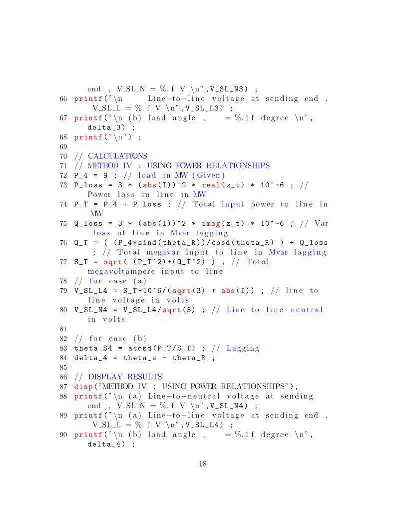
6970 // CALCULATIONS71 // METHOD IV : USING POWER RELATIONSHIPS72 P_4 = 9 ; // l oad i n MW ( Given )73 P_loss = 3 * (abs(I))^2 * real(z_t) * 10^-6 ; //

Power l o s s i n l i n e i n MW74 P_T = P_4 + P_loss ; // Tota l i nput power to l i n e i n

MW75 Q_loss = 3 * (abs(I))^2 * imag(z_t) * 10^-6 ; // Var

l o s s o f l i n e i n Mvar l a g g i n g76 Q_T = ( (P_4*sind(theta_R))/cosd(theta_R) ) + Q_loss

; // Tota l megavar input to l i n e i n Mvar l a g g i n g77 S_T = sqrt( (P_T^2)+(Q_T ^2) ) ; // Tota l

megavoltampere input to l i n e78 // f o r c a s e ( a )79 V_SL_L4 = S_T *10^6/( sqrt (3) * abs(I)) ; // l i n e to

l i n e v o l t a g e i n v o l t s80 V_SL_N4 = V_SL_L4/sqrt (3) ; // Line to l i n e n e u t r a l

i n v o l t s8182 // f o r c a s e ( b )83 theta_S4 = acosd(P_T/S_T) ; // Lagg ing84 delta_4 = theta_s - theta_R ;

8586 // DISPLAY RESULTS87 disp(”METHOD IV : USING POWER RELATIONSHIPS”);88 printf(”\n ( a ) Line−to−n e u t r a l v o l t a g e at s e n d i n g

end , V SL N = %. f V \n”,V_SL_N4) ;

89 printf(”\n ( a ) Line−to− l i n e v o l t a g e at s e n d i n g end ,V SL L = %. f V \n”,V_SL_L4) ;


18

91 printf(”\n”);9293 // CALCULATIONS94 // METHOD V : T r e a t i n g 3− l i n e as 1− l i n e hav ing

hav ing V S and V R r e p r e s e n t l i n e −to− l i n ev o l t a g e s not l i n e −to−n e u t r a l v o l t a g e s

95 // f o r c a s e ( a )96 I_line = (p/2)/( V_RL_L * pf) ; // Power d e l i v e r e d i s

4 . 5 MW97 R_loop = 2*real(z_t) ;

98 X_loop = 2*imag(z_t) ;

99 V_SL_L5 = sqrt( (V_RL_L * cosd(theta_R) + I_line*

R_loop)^2 + (V_RL_L * sind(theta_R) + I_line *

X_loop)^2) ; // l i n e to l i n e v o l t a g e i n V100 V_SL_N5 = V_SL_L5/sqrt (3) ; // l i n e to n e u t r a l

v o l t a g e i n V101102 // f o r c a s e ( b )103 theta_S5 = atand (( V_RL_L * sind(theta_R) + I_line *

X_loop)/( V_RL_L * cosd(theta_R) + I_line*R_loop))

;

104 delta_5 = theta_S5 - theta_R ;

105106 // DISPLAY RESULTS107 disp(”METHOD V : TREATING 3− LINE AS 1− LINE”) ;

108 printf(”\n ( a ) L ine to n e u t r a l v o l t a g e at s e n d i n gend , V SL N = %. f V \n”,V_SL_N5) ;

109 printf(”\n ( a ) L ine to l i n e v o l t a g e at s e n d i n g end ,V SL L = %. f V \n”,V_SL_L5) ;


111 printf(”\n”) ;

112113 printf(”\n NOTE : ERROR : Change i n answer because

r o o t ( 3 ) = 1 . 7 3 i s c o n s i d e r e d i n Textbook ”) ;

114 printf(”\n But he r e s q r t ( 3 ) = 1 . 7 32 0 5 0 8 i sc o n s i d e r e d \n”) ;

19

Scilab code Exa 4.2 calculate percentage voltage regulation using equa-tion



c o n s o l e9

10 // GIVEN DATA11 // f o r c a s e ( a )12 V_S = 14803 ; // s e n d i n g end phase v o l t a g e at no

l oad i n v o l t s . From exa 4 . 113 V_R = 13279.056 ; // r e c e i v i n g end phase v o l t a g e at

f u l l l o ad i n v o l t s . From exa 4 . 11415 // f o r c a s e ( b )16 I_R = 265.78785 ; // Line c u r r e n t i n amperes . From

exa 4 . 117 z_t = 2.48+ %i *6.57 ; // Tota l impedance i n ohm/ phase18 pf = 0.85 ; // power f a c t o r19 theta_R = acosd(pf) ;

2021 // CALCULATIONS22 // f o r c a s e ( a )23 V_reg1 = ( (V_S - V_R)/V_R )*100 ; // p e r c e n t a g e

v o l t a g e r e g u l a t i o n u s i n g equ 4 . 2 92425 // f o r c a s e ( b )

20

26 V_reg2 = (I_R * ( real(z_t) * cosd(theta_R) + imag(

z_t) * sind(theta_R) )/ V_R)*100 ; // p e r c e n t a g ev o l t a g e r e g u l a t i o n u s i n g equ 4 . 3 1


30 printf(”\n ( a ) Pe r c en tage o f v o l t a g e r e g u l a t i o nu s i n g equ 4 . 2 9 = %. 1 f \n”,V_reg1) ;

31 printf(”\n ( b ) Pe r c en tage o f v o l t a g e r e g u l a t i o nu s i n g equ 4 . 3 1 = %. 1 f \n”,V_reg2) ;

3233 printf(”\n NOTE : ERROR : The q u e s t i o n i s with

r e s p e c t to v a l u e s g i v e n i n Exa 4 . 1 not 4 . 5 \n”) ;

Scilab code Exa 4.3 mutual impedance between the feeders



c o n s o l e1011 // GIVEN DATA12 Z_xy = 0.09 + %i*0.3 ; // Mutual impedance between

two p a r a l l e l f e e d e r s i n /mi per phase13 Z_xx = 0.604* exp(%i *50.4* %pi /180) ; // S e l f

impedance o f f e e d e r s i n /mi per phase14 Z_yy = 0.567* exp(%i *52.9* %pi /180) ; // S e l f

impedance o f f e e d e r s i n /mi per phase

21

1516 // SOLUTION17 Z_2 = Z_xx - Z_xy ; // mutual impedance between

f e e d e r s18 Z_4 = Z_yy - Z_xy ; // mutual impedance between

f e e d e r s1920 // DISPLAY RESULTS21 disp(”EXAMPLE : 4 . 3 : SOLUTION :−”) ;

22 printf(”\n Mutual impedance at node 2 , Z 2 = %. 3 f+ j% . 3 f \n”,real(Z_2),imag(Z_2)) ;

23 printf(”\n Mutual impedance at node 4 , Z 4 = %. 3 f+ j% . 3 f \n”,real(Z_4),imag(Z_4)) ;

Scilab code Exa 4.4 calculate A B C D Vs I pf efficiency



c o n s o l e1011 // GIVEN DATA12 V = 138*10^3 ; // t r a n s m i s s i o n l i n e v o l t a g e i n V13 P = 49*10^6 ; // l oad power i n Watts14 pf = 0.85 ; // l a g g i n g power f a c t o r15 Z = 95 * exp(%i*78* %pi /180) ; // l i n e c o n s t a n t s i n

16 Y = 0.001 * exp(%i*90* %pi /180) ; // l i n e c o n s t a n t s

22

i n s i emens1718 // CALCULATIONS19 V_RL_N = V/sqrt (3) ;

20 theta_R = acosd(pf) ;

21 I_R = P/(sqrt (3)*V*pf)*( cosd(theta_R) - %i*sind(

theta_R) ) ; // r e c e i v i n g end c u r r e n t i n ampere2223 // f o r c a s e ( a )24 // A, B, C,D c o n s t a n t s f o r nominal−T c i r c u i t

r e p r e s e n t a t i o n25 A = 1 + (1/2)*Y*Z ;

26 B = Z + (1/4)*Y*Z^2 ;

27 C = Y ;

28 D = A ;

2930 // f o r c a s e ( b )31 P = [A B ; C D] * [V_RL_N ; I_R] ;

32 V_SL_N = P(1,1) ; // Line−to−n e u t r a l Send ing endv o l t a g e i n V

33 V_SL_L = sqrt (3) * abs(V_SL_N) * exp(%i* ( atand(

imag(V_SL_N),real(V_SL_N) ) + 30 )* %pi /180) ; //Line−to− l i n e v o l t a g e i n V

34 // NOTE tha t an a d d i t i o n a l 30 d e g r e e i s added to thea n g l e s i n c e l i n e to l i n e v o l t a g e i s 30 d e g r e e

ahead o f i t s l i n e to n e u t r a l v o l t a g e353637 // f o r c a s e ( c )38 I_S = P(2,1); // Sending end c u r r e n t i n A3940 // f o r c a s e ( d )41 theta_s = atand( imag(V_SL_N),real(V_SL_N) ) - atand

( imag(I_S),real(I_S) ) ;

4243 // f o r c a s e ( e )44 n = (sqrt (3) * V * abs(I_R) * cosd(theta_R)/(sqrt (3)

* abs(I_S) * abs(V_SL_L) * cosd(theta_s) ))*100

23

; // E f f i c i e n c y4546 // DISPLAY RESULTS47 disp(”EXAMPLE : 4 . 4 : SOLUTION :−”) ;

48 printf(”\n ( a ) A c o n s t a n t o f l i n e , A = %. 4 f<%. 1 f \n”,abs(A),atand( imag(A),real(A) )) ;

49 printf(”\n B c o n s t a n t o f l i n e , B = %. 2 f<%. 1 f\n”,abs(B),atand( imag(B),real(B) )) ;

50 printf(”\n C c o n s t a n t o f l i n e , C = %. 3 f<%. 1 f S\n”,abs(C),atand( imag(C),real(C) )) ;

51 printf(”\n D c o n s t a n t o f l i n e , D = %. 4 f<%. 1 f \n”,abs(D),atand( imag(D),real(D) )) ;

52 printf(”\n ( b ) Sending end l i n e −to−n e u t r a l v o l t a g e ,V SL N = %. 1 f<%. 1 f V \n”,abs(V_SL_N),atand( imag

(V_SL_N),real(V_SL_N) )) ;

53 printf(”\n Sending end l i n e −to− l i n e v o l t a g e ,V SL L = %. 1 f<%. 1 f V \n”,abs(V_SL_L),atand( imag(


54 printf(”\n ( c ) s e n d i n g end c u r r e n t , I S = %. 2 f<%. 1 fA \n”,abs(I_S),atand( imag(I_S),real(I_S) )) ;

55 printf(”\n ( d ) s e n d i n g end power f a c t o r , c o s s =%. 3 f \n”,cosd(theta_s)) ;

56 printf(”\n ( e ) E f f i c i e n c y o f t r a n s m i s s i o n , = %. 2f Pe r c en tage \n”,n) ;

5758 printf(”\n NOTE : From A = 0.9536 <0 .6 , magnitude i s

0 . 9 5 3 6 & a n g l e i s 0 . 6 d e g r e e ”) ;

59 printf(”\n ERROR : Change i n answer because r o o t ( 3 )= 1 . 7 3 i s c o n s i d e r e d i n Textbook ”) ;


Scilab code Exa 4.5 calculate A B C D Vs I pf efficiency using nominal pi

24



c o n s o l e1011 // GIVEN DATA12 V = 138*10^3 ; // Transmi s s i on l i n e v o l t a g e i n V13 P = 49*10^6 ; // l oad power i n Watts14 pf = 0.85 ; // l a g g i n g power f a c t o r15 Z = 95 * exp(%i*78* %pi /180) ; // l i n e c o n s t a n t s i n

16 Y = 0.001 * exp(%i*90* %pi /180) ; // l i n e c o n s t a n t si n s i emens

1718 // CALCULATIONS19 V_RL_N = V/sqrt (3) ;


21 I_R = P/(sqrt (3)*V*pf) * ( cosd(theta_R) - %i*sind(

theta_R) ) ; // R e c e i v i n g end c u r r e n t i n A2223 // f o r c a s e ( a )24 // A, B, C,D c o n s t a n t s f o r nominal− c i r c u i t

r e p r e s e n t a t i o n25 A = 1 + (1/2)*Y*Z ;

26 B = Z ;

27 C = Y + (1/4)*(Y^2)*Z ;

28 D = 1 + (1/2)*Y*Z ;


32 V_SL_N = P(1,1) ; // Line−to−n e u t r a l Send ing end

25

v o l t a g e i n V33 V_SL_L = sqrt (3) * abs(V_SL_N) * exp(%i* ( atand(


34 // NOTE tha t an a d d i t i o n a l 30 d e g r e e i s added to thea n g l e s i n c e l i n e −to− l i n e v o l t a g e i s 30 d e g r e e

ahead o f i t s l i n e −to−n e u t r a l v o l t a g e353637 // f o r c a s e ( c )38 I_S = P(2,1); // Sending end c u r r e n t i n A3940 // f o r c a s e ( d )41 theta_s = atand( imag(V_SL_N),real(V_SL_N) ) - atand

( imag(I_S),real(I_S) ) ;

4243 // f o r c a s e ( e )44 n = (sqrt (3) * V * abs(I_R) * cosd(theta_R)/(sqrt (3)

* abs(I_S) * abs(V_SL_L) * cosd(theta_s) ))*100

; // E f f i c i e n c y4546 // DISPLAY RESULTS47 disp(”EXAMPLE : 4 . 5 : SOLUTION :−”) ;









54 printf(”\n ( c ) s e n d i n g end c u r r e n t , I S = %. 2 f<%. 1 f

26

A \n”,abs(I_S),atand( imag(I_S),real(I_S) )) ;

55 printf(”\n ( d ) s e n d i n g end power f a c t o r , c o s s =%. 3 f \n”,cosd(theta_s)) ;

56 printf(”\n ( e ) E f f i c i e n c y o f t r a n s m i s s i o n , = %. 2f Pe r c en tage \n”,n) ;


r o o t ( 3 ) = 1 . 7 3 i s c o n s i d e r e d i n Textbook ”) ;


Scilab code Exa 4.6 calculate A B C D Vs I pf P Ploss n VR Is Vr



c o n s o l e1011 // GIVEN DATA12 V_RL_L = 138*10^3 ; // t r a n s m i s s i o n l i n e v o l t a g e i n

V13 R = 0.1858 // Line c o n s t a n t i n /mi14 f = 60 // f r e q u e n c y i n Hertz15 L = 2.60*10^ -3 // Line c o n s t a n t i n H/mi16 C = 0.012*10^ -6 // Line c o n s t a n t i n F/mi17 pf = 0.85 // Lagg ing power f a c t o r18 P = 50*10^6 // l oad i n VA19 l = 150 // l e n g t h o f 3− t r a n s m i s s i o n l i n e i n mi

27

2021 // CALCULATIONS22 z = R + %i*2* %pi*f*L ; // Impedance per u n i t l e n g t h

i n /mi23 y = %i*2*%pi*C*f ; // Admittance per u n i t l e n g t h i n

S/mi24 g = sqrt(y*z) ; // Propagat i on c o n s t a n t o f l i n e per

u n i t l e n g t h25 g_l = real(g) * l + %i * imag(g) * l ; //

Propagat i on c o n s t a n t o f l i n e26 Z_c = sqrt(z/y) ; // C h a r a c t e r i s t i c impedance o f

l i n e27 V_RL_N = V_RL_L/sqrt (3) ;


29 I_R = P/(sqrt (3)*V_RL_L)*( cosd(theta_R) - %i*sind(

theta_R) ) ; // R e c e i v i n g end c u r r e n t i n A3031 // f o r c a s e ( a )32 // A, B, C,D c o n s t a n t s o f l i n e33 A = cosh(g_l) ;

34 B = Z_c * sinh(g_l) ;

35 C = (1/Z_c) * sinh(g_l) ;

36 D = A ;


40 V_SL_N = P(1,1) ; // Line−to−n e u t r a l Send ing endv o l t a g e i n V

41 V_SL_L = sqrt (3) * abs(V_SL_N) * exp(%i* ( atand(


42 // NOTE tha t an a d d i t i o n a l 30 d e g r e e i s added to thea n g l e s i n c e l i n e −to− l i n e v o l t a g e i s 30 d e g r e e

ahead o f i t s l i n e −to−n e u t r a l v o l t a g e4344 // f o r c a s e ( c )45 I_S = P(2,1); // Sending end c u r r e n t i n A46

28

47 // f o r c a s e ( d )48 theta_s = atand( imag(V_SL_N),real(V_SL_N) ) - atand

( imag(I_S),real(I_S) ) ; // Sending−end p f4950 // For c a s e ( e )51 P_S = sqrt (3) * abs(V_SL_L) * abs(I_S) * cosd(

theta_s) ; // Sending end power5253 // For c a s e ( f )54 P_R = sqrt (3)*abs(V_RL_L)*abs(I_R)*cosd(theta_R) ;

// R e c e i v i n g end power55 P_L = P_S - P_R ; // Power l o s s i n l i n e5657 // For c a s e ( g )58 n = (P_R/P_S)*100 ; // Transmi s s i on l i n e e f f i c i e n c y5960 // For c a s e ( h )61 reg = (( abs(V_SL_N) - V_RL_N )/V_RL_N )*100 ; //

Pe r c en tage o f v o l t a g e r e g u l a t i o n6263 // For c a s e ( i )64 Y = y * l ; // u n i t i s S65 I_C = (1/2) * Y * V_SL_N ; // Sending end c h a r g i n g

c u r r e n t i n A6667 // For c a s e ( j )68 Z = z * l ;

69 V_RL_N0 = V_SL_N - I_C*Z ;

70 V_RL_L0 = sqrt (3) * abs(V_RL_N0) * exp(%i* ( atand(

imag(V_RL_N0),real(V_RL_N0) ) + 30 )* %pi /180) ;

// Line−to− l i n e v o l t a g e at r e c e i v i n g end i n V7172 // DISPLAY RESULTS73 disp(”EXAMPLE : 4 . 6 : SOLUTION :−”) ;



29







80 printf(”\n ( c ) send ing−end c u r r e n t , I S = %. 2 f<%. 2 fA \n”,abs(I_S),atand( imag(I_S),real(I_S) )) ;

81 printf(”\n ( d ) send ing−end power f a c t o r , c o s s =%. 4 f \n”,cosd(theta_s)) ;

82 printf(”\n ( e ) send ing−end power , P S = %. 5 e W \n”,P_S) ;

83 printf(”\n ( f ) Power l o s s i n l i n e , P L = %. 5 e W \n”,P_L) ;

84 printf(”\n ( g ) Transmi s s i on l i n e E f f i c i e n c y , = %. 1 f Pe r c en tage \n”,n) ;

85 printf(”\n ( h ) Pe r c en tage o f v o l t a g e r e g u l a t i o n = %. 1 f Pe r c en tage \n”,reg) ;

86 printf(”\n ( i ) Sending−end c h a r g i n g c u r r e n t at nol oad , I C = %. 2 f A \n”,abs(I_C)) ;

87 printf(”\n ( j ) Rece iv ing−end v o l t a g e r i s e at no l oad, V RL N = %. 2 f<%. 2 f V \n”,abs(V_RL_N0),atand(

imag(V_RL_N0),real(V_RL_N0)));

88 printf(”\n Line−to− l i n e v o l t a g e at r e c e i v i n g endat no l oad , V RL L = %. 2 f<%. 2 f V \n”,abs(V_RL_L0

),atand(imag(V_RL_L0),real(V_RL_L0)));


r o o t ( 3 ) = 1 . 7 3 i s c o n s i d e r e d i n Textbook & changei n & v a l u e s ”) ;


30

Scilab code Exa 4.7 find equivalent pi T circuit and Nominal pi T circuit

12 // ELECTRIC POWER TRANSMISSION SYSTEM ENGINEERING

ANALYSIS AND DESIGN3 // TURAN GONEN4 // CRC PRESS5 // SECOND EDITION67 // CHAPTER : 4 : OVERHEAD POWER TRANSMISSION89 // EXAMPLE : 4 . 7 :

10 clear ; clc ; close ; // C l ea r the work space andc o n s o l e

1112 // GIVEN DATA13 R = 0.1858 // Line c o n s t a n t i n /mi14 f = 60 // f r e q u e n c y i n Hertz15 L = 2.60*10^ -3 // Line c o n s t a n t i n H/mi16 C = 0.012*10^ -6 // Line c o n s t a n t i n F/mi17 l = 150 // l e n g t h o f 3− t r a n s m i s s i o n l i n e i n mi1819 // CALCULATIONS20 z = R + %i*2* %pi*f*L ; // Impedance per u n i t l e n g t h



u n i t l e n g t h23 g_l = real(g) * l + %i * imag(g) * l ; //

Propagat i on c o n s t a n t o f l i n e24 Z_c = sqrt(z/y) ; // C h a r a c t e r i s t i c impedance o f

l i n e25

31

26 A = cosh(g_l) ;

27 B = Z_c * sinh(g_l) ;

28 C = (1/Z_c) * sinh(g_l) ;

29 D = A ;

30 Z_pi = B ;

31 Y_pi_by2 = (A-1)/B ; // Unit i n Siemens32 Z = l * z ; // u n i t i n ohms33 Y = y * l ;

34 Y_T = C ;

35 Z_T_by2 = (A-1)/C ; // Unit i n3637 // DISPLAY RESULTS38 disp(”EXAMPLE : 4 . 7 : SOLUTION :−”) ;

39 printf(”\n FOR EQUIVALENT− CIRCUIT ”) ;

40 printf(”\n Z = B = %. 2 f<%. 2 f \n”,abs(Z_pi),atand( imag(Z_pi),real(Z_pi) )) ;

41 printf(”\n Y /2 = %. 6 f<%. 2 f S \n”,abs(Y_pi_by2),atand( imag(Y_pi_by2),real(Y_pi_by2) )) ;

42 printf(”\n FOR NOMINAL− CIRCUIT ”) ;

43 printf(”\n Z = %. 3 f<%. 2 f \n”,abs(Z),atand( imag

(Z),real(Z) )) ;

44 printf(”\n Y/2 = %. 6 f<%. 1 f S \n”,abs(Y/2),atand(imag(Y/2),real(Y/2) )) ;

45 printf(”\n FOR EQUIVALENT−T CIRCUIT ”) ;

46 printf(”\n Z T/2 = %. 2 f<%. 2 f \n”,abs(Z_T_by2),atand( imag(Z_T_by2),real(Z_T_by2) )) ;

47 printf(”\n Y T = C = %. 5 f<%. 2 f S \n”,abs(Y_T),atand( imag(Y_T),real(Y_T) )) ;

48 printf(”\n FOR NOMINAL−T CIRCUIT ”) ;

49 printf(”\n Z/2 = %. 2 f<%. 2 f \n”,abs(Z/2),atand(imag(Z/2),real(Z/2) )) ;

50 printf(”\n Y = %. 6 f<%. 1 f S \n”,abs(Y),atand( imag(

Y),real(Y) )) ;

32

Scilab code Exa 4.8 calculate attenuation phase change lamda v Vir VrrVr Vis Vrs Vs



c o n s o l e1011 // GIVEN DATA12 V_RL_L = 138*10^3 ; // t r a n s m i s s i o n l i n e v o l t a g e i n

V13 R = 0.1858 // Line c o n s t a n t i n /mi14 f = 60 // f r e q u e n c y i n Hertz15 L = 2.60*10^ -3 // Line c o n s t a n t i n H/mi16 C = 0.012*10^ -6 // Line c o n s t a n t i n F/mi17 pf = 0.85 // Lagg ing power f a c t o r18 P = 50*10^6 // l oad i n VA19 l = 150 // l e n g t h o f 3− t r a n s m i s s i o n l i n e i n mi2021 // CALCULATIONS22 // For c a s e ( a )23 z = R + %i*2* %pi*f*L ; // Impedance per u n i t l e n g t h



u n i t l e n g t h2627 // For c a s e ( b )28 lamda = (2 * %pi)/imag(g) ; // Wavelength o f

p r o p a g a t i o n i n mi

33

29 V = lamda * f ; // V e l o c i t y o f p r o p a g a t i o n i n mi/ s e c3031 // For c a s e ( c )32 Z_C = sqrt(z/y) ;

33 V_R = V_RL_L/sqrt (3) ;


35 I_R = P/(sqrt (3)*V_RL_L) * ( cosd(theta_R) - %i*sind

(theta_R) ) ; // R e c e i v i n g end c u r r e n t i n A36 V_R_incident = (1/2)*(V_R + I_R*Z_C) ; // I n c i d e n t

v o l t a g e at r e c e i v i n g end i n V37 V_R_reflected = (1/2)*(V_R - I_R*Z_C) ; // R e f l e c t e d

v o l t a g e at r e c e i v i n g end i n V3839 // For c a s e ( d )40 V_RL_N = V_R_incident + V_R_reflected ; // Line−to−

n e u t r a l v o l t a g e at r e c e i v i n g end i n V41 V_RL_L = sqrt (3)*V_RL_N // R e c e i v i n g end Line

v o l t a g e i n V4243 // For c a s e ( e )44 g_l = real(g) * l + %i * imag(g) * l ; //

Propagat i on c o n s t a n t o f l i n e45 a = real(g) ; // a = i s the a t t e n u a t i o n c o n s t a n t46 b = imag(g) ; // b = i s the phase c o n s t a n t47 V_S_incident = (1/2) * (V_R+I_R*Z_C) * exp(a*l) *

exp(%i*b*l) ; // I n c i d e n t v o l t a g e at s e n d i n g endi n V

48 V_S_reflected = (1/2) * (V_R -I_R*Z_C) * exp(-a*l) *

exp(%i*(-b)*l) ; // R e f l e c t e d v o l t a g e at s e n d i n gend i n V

4950 // For c a s e ( f )51 V_SL_N = V_S_incident + V_S_reflected ; // Line−to−

n e u t r a l v o l t a g e at s e n d i n g end i n V52 V_SL_L = sqrt (3)*V_SL_N ; // s e n d i n g end Line

v o l t a g e i n V5354 // DISPLAY RESULTS

34

55 disp(”EXAMPLE : 4 . 8 : SOLUTION :−”) ;

56 printf(”\n ( a ) At t enua t i on c o n s t a n t , = %. 4 f Np/mi \n”,real(g)) ;

57 printf(”\n Phase change cons tant , = %. 4 f rad /mi \n”,imag(g)) ;

58 printf(”\n ( b ) Wavelength o f p r o p a g a t i o n = %. 2 f mi \n”,lamda) ;

59 printf(”\n v e l o c i t y o f p r o p a g a t i o n = %. 2 f mi/ s \n”,V) ;

60 printf(”\n ( c ) I n c i d e n t v o l t a g e r e c e i v i n g end , V R(i n c i d e n t ) = %. 2 f<%. 2 f V \n”,abs(V_R_incident),atan(imag(V_R_incident),real(V_R_incident))*(180/

%pi));

61 printf(”\n R e c e i v i n g end r e f l e c t e d v o l t a g e , V R( r e f l e c t e d ) = %. 2 f<%. 2 f V \n”,abs(V_R_reflected),atan(imag(V_R_reflected),real(V_R_reflected))

*(180/ %pi)) ;

62 printf(”\n ( d ) L ine v o l t a g e at r e c e i v i n g end ,V RL L = %d V \n”,V_RL_L) ;

63 printf(”\n ( e ) I n c i d e n t v o l t a g e at s e n d i n g end , V S( i n c i d e n t ) = %. 2 f<%. 2 f V \n”,abs(V_S_incident),atan(imag(V_S_incident),real(V_S_incident))*(180/

%pi)) ;

64 printf(”\n R e f l e c t e d v o l t a g e at s e n d i n g end ,V S ( r e f l e c t e d ) = %. 2 f<%. 2 f V \n”,abs(V_S_reflected),atan(imag(V_S_reflected),real(

V_S_reflected))*(180/ %pi)) ;

65 printf(”\n ( f ) L ine v o l t a g e at s e n d i n g end , V SL L= %. 2 f V \n”,abs(V_SL_L)) ;

Scilab code Exa 4.9 calculate SIL


2 // TURAN GONEN

35

3 // CRC PRESS4 // SECOND EDITION56 // CHAPTER : 4 : OVERHEAD POWER TRANSMISSION78 // EXAMPLE : 4 . 9 :9 clear ; clc ; close ; // C l ea r the work space and

c o n s o l e1011 // GIVEN DATA12 L = 2.60 * 10^-3 ; // Induc tance o f l i n e i n H/mi13 R = 0.1858 ; // R e s i s t a n c e o f l i n e i n /mi14 C = 0.012 * 10^-6 ; // Capac i t ance i n F/mi15 kV = 138 ; // Transmi s s i on l i n e v o l t a g e i n kV16 Z_c1 = 469.60085 // C h a r a c t e r i s t i c impedance o f l i n e

i n . Obtained from example 4 . 61718 // CALCULATIONS19 Z_c = sqrt(L/C) ; // Approximate v a l u e o f s u r g e

Impedance o f l i n e i n ohm20 SIL = kV^2/ Z_c ; // Approximate Surge impedance

l o a d i n g i n MW21 SIL1 = kV^2/ Z_c1 ; // Exact v a l u e o f SIL i n MW2223 // DISPLAY RESULTS24 disp(”EXAMPLE : 4 . 9 : SOLUTION :−”) ;

25 printf(”\n Approximate v a l u e o f SIL o f t r a n s m i s s i o nl i n e , SIL app = %. 3 f MW\n”,SIL) ;

26 printf(”\n Exact v a l u e o f SIL o f t r a n s m i s s i o n l i n e ,S I L e x a c t = %. 3 f MW\n”,SIL1) ;

Scilab code Exa 4.10 determine equ A B C D constant


36

2 // TURAN GONEN3 // CRC PRESS4 // SECOND EDITION56 // CHAPTER : 4 : OVERHEAD POWER TRANSMISSION78 // EXAMPLE : 4 . 1 0 :9 clear ; clc ; close ; // C l ea r the work space and

c o n s o l e1011 // GIVEN DATA12 Z_1 = 10 * exp(%i*(30)*%pi /180) ; // Impedance i n13 Z_2 = 40 * exp(%i*(-45)*%pi /180) ; // Impedance i n

1415 // CALCULATIONS16 P = [1 ,Z_1 ; 0 , 1]; // For network 117 Y_2 = 1/Z_2 ; // u n i t i s S18 Q = [1 0 ; Y_2 1]; // For network 219 EQ = P * Q ;

2021 // DISPLAY RESULTS22 disp(”EXAMPLE : 4 . 1 0 : SOLUTION :−”) ;

23 printf(”\n E q u i v a l e n t A , B , C , D c o n s t a n t s a r e \n”) ;

24 printf(”\n A eq = %. 3 f<%. 1 f \n”,abs( EQ(1,1) ),atand

( imag(EQ(1,1)),real(EQ(1,1)) )) ;

25 printf(”\n B eq = %. 3 f<%. 1 f \n”,abs( EQ(1,2) ),atand

( imag(EQ(1,2)),real(EQ(1,2)) )) ;

26 printf(”\n C eq = %. 3 f<%. 1 f \n”,abs( EQ(2,1) ),atand

( imag(EQ(2,1)),real(EQ(2,1)) )) ;

27 printf(”\n D eq = %. 3 f<%. 1 f \n”,abs( EQ(2,2 )),atand

( imag(EQ(2,2)),real(EQ(2,2)) )) ;

Scilab code Exa 4.11 determine equ A B C D constant

37



c o n s o l e1011 // GIVEN DATA12 Z_1 = 10*exp(%i*(30)*%pi /180) ; // Impedance i n13 Z_2 = 40*exp(%i*(-45)*%pi /180) ; // Impedance i n14 Y_2 = 1/Z_2 ;

15 A_1 = 1 ;

16 B_1 = Z_1 ;

17 C_1 = 0 ;

18 D_1 = 1 ;

19 A_2 = 1 ;

20 B_2 = 0 ;

21 C_2 = Y_2 ;

22 D_2 = 1 ;

2324 // CALCULATIONS25 P = [A_1 B_1 ; C_1 D_1]; // For network 126 Q = [A_2 B_2 ; C_2 D_2]; // For network 227 A_eq = ( A_1*B_2 + A_2*B_1 )/( B_1 + B_2 ) ; //

Constant A28 B_eq = ( B_1*B_2 )/(B_1 + B_2) ; // Constant B29 C_eq = C_1 + C_2 + ( (A_1 - A_2) * (D_2 -D_1)/(B_1 +

B_2) ) ; // Constant C30 D_eq = ( D_1*B_2 + D_2*B_1 )/(B_1+B_2) ; // Constant

D3132 // DISPLAY RESULTS33 disp(”EXAMPLE : 4 . 1 1 : SOLUTION :−”) ;

38

34 printf(”\n E q u i v a l e n t A , B , C , D c o n s t a n t s a r e \n”) ;

35 printf(”\n A eq = %. 2 f<%. f \n”,abs(A_eq),atand( imag

(A_eq),real(A_eq) )) ;

36 printf(”\n B eq = %. 2 f<%. f \n”,abs(B_eq),atand( imag

(B_eq),real(B_eq) )) ;

37 printf(”\n C eq = %. 3 f<%. f \n”,abs(C_eq),atand( imag

(C_eq),real(C_eq) )) ;

38 printf(”\n D eq = %. 2 f<%. f \n”,abs(D_eq),atand( imag

(D_eq),real(D_eq) )) ;

Scilab code Exa 4.12 calculate Is Vs Zin P var



c o n s o l e1011 // GIVEN DATA12 Z = 2.07 + 0.661 * %i ; // Line impedance i n13 V_L = 2.4 * 10^3 ; // Line v o l t a g e i n V14 p = 200 * 10^3; // Load i n VA15 pf = 0.866 ; // Lagg ing power f a c t o r1617 // CALCULATIONS18 // f o r c a s e ( a )19 A = 1 ;

20 B = Z ;

39

21 C = 0 ;

22 D = A ;

23 theta = acosd(pf) ;

24 S_R = p * ( cosd(theta) + %i * sind(theta) ) ; //R e c e i v i n g end power i n VA

25 I_L1 = S_R/V_L ;

26 I_L = conj(I_L1) ;

27 I_S = I_L ; // s e n d i n g end c u r r e n t i n A28 I_R = I_S ; // R e c e i v i n g end c u r r e n t i n A2930 // f o r c a s e ( b )31 Z_L = V_L/I_L ; // Impedance i n32 V_R = Z_L * I_R ;

33 V_S = A * V_R + B * I_R ; // s e n d i n g end v o l t a g e i nV

34 P = [A B ;C D] * [V_R ; I_R] ;

3536 // f o r c a s e ( c )37 V_S = P(1,1) ;

38 I_S = P(2,1) ;

39 Z_in = V_S/I_S ; // Input impedance i n4041 // f o r c a s e ( d )42 S_S = V_S * conj(I_S) ;

43 S_L = S_S - S_R ; // Power l o s s o f l i n e i n VA4445 // DISPLAY RESULTS46 disp(”EXAMPLE : 4 . 1 2 : SOLUTION :−”) ;

47 printf(”\n ( a ) Sending−end c u r r e n t , I S = %. 2 f<%. 2 fA \n”,abs(I_S),atand( imag(I_S),real(I_S) )) ;

48 printf(”\n ( b ) Sending−end v o l t a g e , V S = %. 2 f<%. 2 fV \n”,abs(V_S),atand( imag(V_S),real(V_S) )) ;

49 printf(”\n ( c ) Input impedance , Z i n = %. 2 f<%. 2 f\n”,abs(Z_in),atand( imag(Z_in),real(Z_in) )) ;

50 printf(”\n ( d ) Real power l o s s i n l i n e , S L = %. 2 fW \n”,real(S_L)) ;

51 printf(”\n R e a c t i v e power l o s s i n l i n e , S L = %. 2 f var \n”,imag(S_L)) ;

40

Scilab code Exa 4.13 calculate SIL Pmax Qc Vroc



c o n s o l e1011 // GIVEN DATA12 KV = 345 ; // Transmi s s i on l i n e v o l t a g e i n kV13 V_R = KV ;

14 V_S = KV ;

15 x_L = 0.588 ;// I n d u c t i v e r e a c t a n c e i n /mi/ phase16 b_c = 7.20*10^ -6 ;// s u s c e p t a n c e S phase to n e u t r a l

per phase17 l = 200 ;// Tota l l i n e l e n g t h i n mi1819 // CALCULATIONS20 // f o r c a s e ( a )21 x_C = 1/b_c ;// /mi/ phase22 Z_C = sqrt(x_C * x_L) ;

23 SIL = KV^2/Z_C ; // Surge impedance l o a d i n g i n MVA/mi . [ 1MVA = 1MW]

24 SIL1 = (KV^2/ Z_C) * l ; // Surge impedance l o a d i n go f l i n e i n MVA . [ 1MVA = 1MW]

2526 // f o r c a s e ( b )27 delta = 90 ; // Max 3− t h e o r e t i c a l s teady−s t a t e

41

power f l o w l i m i t o c c u r s f o r = 90 d e g r e e28 X_L = x_L * l ; // I n d u c t i v e r e a c t a n c e / phase29 P_max = V_S * V_R * sind(delta)/(X_L) ;

3031 // f o r c a s e ( c )32 Q_C = V_S^2 * (b_c * l/2) + V_R^2 *( b_c * l/2) ; //

Tota l 3− magne t i z i ng var i n Mvar3334 // f o r c a s e ( d )35 g = %i * sqrt(x_L/x_C) ; // rad /mi36 g_l = g * l ; // rad37 V_R_oc = V_S / cosh(g_l) ; // Open−c i r c u i t r e c e i v i n g

−end v o l t a g e i n kV38 X_C = x_C * 2 / l ;

39 V_R_oc1 = V_S * ( - %i * X_C/( - %i * X_C + %i * X_L

) ) ; // A l e r n a t i v e method to f i n d Open−c i r c u i tr e c e i v i n g −end v o l t a g e i n kV


43 printf(”\n ( a ) Tota l 3− SIL o f l i n e , SIL = %. 2 fMVA/mi \n”,SIL) ;

44 printf(”\n Tota l 3− SIL o f l i n e f o r t o t a l l i n el e n g t h , SIL = %. 2 f MVA \n”,SIL1) ;

45 printf(”\n ( b ) Maximum 3− t h e o r t i c a l s teady−s t a t epower f l o w l i m i t , P max = %. 2 f MW \n”,P_max) ;

46 printf(”\n ( c ) Tota l 3− magne t i z i ng var g e n e r a t i o nby l i n e c a p a c i t a n c e , Q C = %. 2 f Mvar \n”,Q_C) ;

47 printf(”\n ( d ) Open−c i r c u i t r e c e i v i n g −end v o l t a g e i fl i n e i s open at r e c e i v i n g end , V R oc = %. 2 f kV\n”,V_R_oc) ;

48 printf(”\n From a l t e r n a t i v e method , ”) ;

49 printf(”\n Open−c i r c u i t r e c e i v i n g −end v o l t a g e i fl i n e i s open at r e c e i v i n g end , V R oc = %. 2 f kV\n”,V_R_oc1) ;

42

Scilab code Exa 4.14 calculate SIL Pmax Qc cost Vroc



c o n s o l e1011 // GIVEN DATA12 KV = 345 ; // Transmi s s i on l i n e v o l t a g e i n kV13 V_R = KV ; // Sending end v o l t a g e i n kV14 x_L = 0.588 ;// I n d u c t i v e r e a c t a n c e i n /mi/ phase15 b_c = 7.20*10^ -6 ;// s u s c e p t a n c e S phase to n e u t r a l

per phase16 l = 200 ;// Tota l l i n e l e n g t h i n mi17 per = 60/100 ; // 2 shunt r e a c t o r s absorb 60% o f

t o t a l 3− magne t i z i ng var18 cost = 10 ; // c o s t o f each r e a c t o r i s $10 /kVA1920 // CALCULATIONS21 // For c a s e ( a )22 x_C = 1/b_c ;// /mi/ phase23 Z_C = sqrt(x_C * x_L) ;

24 SIL = KV^2/Z_C ; // Surge impedance l o a d i n g i n MVA/mi

25 SIL1 = (KV^2/ Z_C) * l ; // Surge impedance l o a d i n go f l i n e i n MVA . [ 1MVA = 1MW]

26

43

27 // For c a s e ( b )28 delta = 90 ; // Max 3− t h e o r e t i c a l s teady−s t a t e

power f l o w l i m i t o c c u r s f o r = 90 d e g r e e29 V_S = V_R ; // s e n d i n g end v o l t a g e i n kV30 X_L = x_L * l ; // I n d u c t i v e r e a c t a n c e / phase31 P_max = V_S * V_R * sind(delta)/(X_L) ;

3233 // For c a s e ( c )34 Q_C = V_S^2 * (b_c * l/2) + V_R^2 *( b_c * l/2) ; //

Tota l 3− magne t i z i ng var i n Mvar35 Q = (1/2) * per * Q_C ; // 3− megavoltampere

r a t i n g o f each r e a c t o r . Q = ( 1 / 2 ) ∗Q L3637 // For c a s e ( d )38 Q_L1 = Q * 10^3 ; // Tota l 3− magne t i z i ng var i n

Kvar39 T_cost = Q_L1 * cost ; // Cost o f each r e a c t o r i n $4041 // For c a s e ( e )42 g = %i * sqrt(x_L * (1-per)/x_C) ; // rad /mi43 g_l = g * l ; // rad44 V_R_oc = V_S/cosh(g_l) ; // Open c i r c u i t r e c e i v i n g −

end v o l t a g e i n kV45 X_L = x_L *l ;

46 X_C = (x_C * 2) / (l * (1 - per)) ;

47 V_R_oc1 = V_S * ( -%i*X_C/(-%i*X_C + %i*X_L) ) ; //A l e r n a t i v e method to f i n d Open−c i r c u i t r e c e i v i n g −end v o l t a g e i n kV


51 printf(”\n ( a ) Tota l 3−phase SIL o f l i n e , SIL = %. 2f MVA/mi \n”,SIL) ;

52 printf(”\n Tota l 3− SIL o f l i n e f o r t o t a l l i n el e n g t h , SIL = %. 2 f MVA \n”,SIL1) ;

53 printf(”\n ( b ) Maximum 3−phase t h e o r t i c a l power f l o w, P max = %. 2 f MW \n”,P_max) ;

54 printf(”\n ( c ) 3−phase MVA r a t i n g o f each r e a c t o r ,

44

( 1 / 2 ) Q L = %. 2 f MVA \n”,Q) ;

55 printf(”\n ( d ) Cost o f each r e a c t o r at $10 /kVA = $ %. 2 f \n”,T_cost) ;

56 printf(”\n ( e ) Open c i r c u i t r e c e i v i n g v o l t a g e ,V Roc= %. 2 f kV \n”,V_R_oc) ;

57 printf(”\n From a l t e r n a t i v e method , ”) ;

58 printf(”\n Open−c i r c u i t r e c e i v i n g −end v o l t a g e i fl i n e i s open at r e c e i v i n g end , V R oc = %. 2 f kV\n”,V_R_oc1) ;

Scilab code Exa 4.15 calculate La XL Cn Xc



c o n s o l e1011 // GIVEN DATA12 D_12 = 26 ; // d i s t a n c e s i n f e e t13 D_23 = 26 ; // d i s t a n c e s i n f e e t14 D_31 = 52 ; // d i s t a n c e s i n f e e t15 d = 12 ; // D i s t a n c e b/w 2 s u b c o n d u c t o r s i n i n c h e s16 f = 60 ; // f r e q u e n c y i n Hz17 kv = 345 ; // v o l t a g e base i n kv18 p = 100 ; // Power base i n MVA19 l = 200 ; // l e n g t h o f l i n e i n km2021 // CALCULATIONS

45

22 // For c a s e ( a )23 D_S = 0.0435 ; // from A. 3 Appendix A . Geometr ic

mean r a d i u s i n f e e t24 D_bS = sqrt(D_S * 0.3048 * d * 0.0254) ; // GMR o f

bundled conduc to r i n m . [ 1 f t = 0 . 3 0 4 8 m ; 1 in ch= 0 . 0 2 5 4 m]

25 D_eq = (D_12 * D_23 * D_31 * 0.3048^3) ^(1/3) ; //Equ GMR i n meter

26 L_a = 2 * 10^-7 * log(D_eq/D_bS); // Induc tance i n H/ meter

2728 // For c a s e ( b )29 X_L = 2 * %pi * f * L_a ; // i n d u c t i v e r e a c t a n c e /

phase i n ohms/m30 X_L0 = X_L * 10^3 ; // i n d u c t i v e r e a c t a n c e / phase i n

ohms/km31 X_L1 = X_L0 * 1.609 ;// i n d u c t i v e r e a c t a n c e / phase i n

ohms/mi [ 1 mi = 1 . 6 0 9 km ]3233 // For c a s e ( c )34 Z_B = kv^2 / p ; // Base impedance i n35 X_L2 = X_L0 * l/Z_B ; // S e r i e s r e a c t a n c e o f l i n e i n

pu3637 // For c a s e ( d )38 r = 1.293*0.3048/(2*12) ; // r a d i u s i n m . o u t s i d e

d i amete r i s 1 . 2 9 3 in ch g i v e n i n A. 339 D_bsC = sqrt(r * d * 0.0254) ;

40 C_n = 55.63 * 10^ -12/ log(D_eq/D_bsC) ; //c a p a c i t a n c e o f l i n e i n F/m

4142 // For c a s e ( e )43 X_C = 1/( 2 * %pi * f * C_n ) ; // c a p a c i t i v e

r e a c t a n c e i n ohm−m44 X_C0 = X_C * 10^-3 ; // c a p a c i t i v e r e a c t a n c e i n ohm−

km45 X_C1 = X_C0 /1.609 ; // c a p a c i t i v e r e a c t a n c e i n ohm−

mi

46


49 printf(”\n ( a ) Average i n d u c t a n c e per phase , L a =%. 4 e H/m \n”,L_a) ;

50 printf(”\n ( b ) I n d u c t i v e r e a c t a n c e per phase , X L =%. 4 f /km \n”,X_L0) ;

51 printf(”\n I n d u c t i v e r e a c t a n c e per phase , X L =%. 4 f /mi \n”,X_L1) ;

52 printf(”\n ( c ) S e r i e s r e a c t a n c e o f l i n e , X L = %. 4 fpu \n”,X_L2) ;

53 printf(”\n ( d ) Line−to−n e u t r a l c a p a c i t a n c e o f l i n e ,C n = %. 4 e F/m \n”,C_n);

54 printf(”\n ( e ) C a p a c i t i v e r e a c t a n c e to n e u t r a l o fl i n e , X C = %. 3 e −km \n”,X_C0) ;

55 printf(”\n C a p a c i t i v e r e a c t a n c e to n e u t r a l o fl i n e , X C = %. 3 e −mi \n”,X_C1) ;

47

Chapter 5

UNDERGROUND POWERTRANSMISSION AND GASINSULATEDTRANSMISSION LINES

Scilab code Exa 5.1 calculate Emax Emin r


2 // TURAN GONEN3 // CRC PRESS4 // SECOND EDITION56 // CHAPTER : 5 : UNDERGROUND POWER TRANSMISSION AND

GAS−INSULATED TRANSMISSION LINES78 // EXAMPLE : 5 . 1 :9 clear ; clc ; close ; // C l ea r the work space and

c o n s o l e1011 // GIVEN DATA12 d = 2 ; // Diameter o f conduc to r i n cm

48

13 D = 5 ; // I n s i d e d i amete r o f l e a d shea th i n cm14 V = 24.9 ; // Line−to−n e u t r a l v o l t a g e i n kV1516 // CALCULATIONS17 // For c a s e ( a )18 r = d/2 ;

19 R = D/2 ;

20 E_max = V/( r * log(R/r) ) ; // Maximum e l e c t r i cs t r e s s i n kV/cm

21 E_min = V/( R * log(R/r) ) ; // Minimum e l e c t r i cs t r e s s i n kV/cm

2223 // For c a s e ( b )24 r_1 = R/2.718 ; // Optimum conduc to r r a d i u s i n cm .

From equ 5 . 1 525 E_max1 = V/( r_1 * log(R/r_1) ) ; // Min v a l u e o f

max s t r e s s i n kV/cm2627 // DISPLAY RESULTS28 disp(”EXAMPLE : 5 . 1 : SOLUTION :−”) ;

29 printf(”\n ( a ) Maximum v a l u e o f e l e c t r i c s t r e s s ,E max = %. 2 f kV/cm \n”,E_max) ;

30 printf(”\n Minimum v a l u e o f e l e c t r i c s t r e s s ,E min = %. 2 f kV/cm \n”,E_min) ;

31 printf(”\n ( b ) Optimum v a l u e o f conduc to r r a d i u s , r= %. 2 f cm \n”,r_1) ;

32 printf(”\n Minimum v a l u e o f maximum s t r e s s ,E max = %. 2 f kV/cm \n”,E_max1) ;

Scilab code Exa 5.2 calculate potential gradient E1


2 // TURAN GONEN3 // CRC PRESS

49

4 // SECOND EDITION56 // CHAPTER : 5 : UNDERGROUND POWER TRANSMISSION AND


c o n s o l e1011 // GIVEN DATA12 r = 1 ; // Radius o f conduc to r i n cm13 t_1 = 2 ; // Th i ckne s s o f i n s u l a t i o n l a y e r i n cm14 r_1 = r + t_1 ;

15 r_2 = 2 ; // Th i ckne s s o f i n s u l a t i o n l a y e r i n cm .r 2 = t 1 = t 2

16 R = r_1 + r_2 ;

17 K_1 = 4 ; // I n n e r l a y e r D i e l e c t r i c c o n s t a n t18 K_2 = 3 ; // Outer l a y e r D i e l e c t r i c c o n s t a n t19 kv = 19.94 ; // p o t e n t i a l d i f f e r e n c e b/w i n n e r &

o u t e r l e a d shea th i n kV2021 // CALCULATIONS22 // E 1 = 2q /( r ∗K 1 ) & E 2 = 2q /( r 1 ∗K 2 ) . Let E =

E 1 / E 223 E = ( r_1 * K_2 )/( r * K_1 ) ; // E = E 1 / E 224 V_1 = poly(0, ’ V 1 ’ ) ; // d e f i n i n g unknown V 125 E_1 = V_1/( r * log(r_1/r) ) ;

26 V_2 = poly(0, ’ V 2 ’ ) ; // d e f i n i n g unknown V 227 V_2 = kv - (V_1) ;

28 E_2 = V_2/( r_1 * log(R/r_1) ) ;

29 E_3 = E_1/E_2 ;

30 // Equat ing E = E 3 . we g e t the v a l u e o f V 131 V_1 = 12.30891068 ; // Vo l tage i n kV32 E_1s = V_1/( r * log(r_1/r) ) ; // P o t e n t i a l

g r a d i e n t at s u r f a c e o f conduc to r i n kV/cm . E 1 =E 1s

3334 // DISPLAY RESULTS

50


36 printf(”\n P o t e n t i a l g r a d i e n t at the s u r f a c e o fconduc to r , E 1 = %. 2 f kV/cm \n”,E_1s) ;

Scilab code Exa 5.3 calculate Ri Power loss




c o n s o l e1011 // GIVEN DATA12 D = 1.235 ; // I n s i d e d i amete r o f shea th i n in ch13 d = 0.575 ; // Conductor d i amete r i n in ch14 kv = 115 ; // Vo l tage i n kV15 l = 6000 ; // Length o f c a b l e i n f e e t16 r_si = 2000 ; // s p e c i f i c i n s u l a t i o n r e s i s t a n c e i s

2000 M /1000 f t . From Table 5 . 21718 // CALCULATIONS19 // For c a s e ( a )20 r_si0 = r_si * l/1000 ;

21 R_i = r_si0 * log10 (D/d) ; // Tota l I n s u l a t i o nr e s i s t a n c e i n M

2223 // For c a s e ( b )24 P = kv^2/R_i ; // Power l o s s due to l e a k a g e c u r r e n t

51

i n W2526 // DISPLAY RESULTS27 disp(”EXAMPLE : 5 . 3 : SOLUTION :−”) ;

28 printf(”\n ( a ) Tota l i n s u l a t i o n r e s i s t a n c e at 60d e g r e e F , R i= %. 2 f M \n”,R_i) ;

29 printf(”\n ( b ) Power l o s s due to l e a k a g e c u r r e n t , Vˆ2/ R i = %. 4 f W \n”,P) ;

3031 printf(”\n NOTE : ERROR : Mistake i n t ex tbook c a s e (

a ) \n”) ;

Scilab code Exa 5.4 calculate charging current Ic




c o n s o l e1011 // GIVEN DATA12 C_a = 2 * 10^-6 ; // Capac i t ance b/w two c o n d u c t o r s

i n F/mi13 l = 2 ; // l e n g t h i n mi14 f = 60 ; // Frequency i n Hz15 V_L_L = 34.5 * 10^3 ; // Line−to− l i n e v o l t a g e i n V1617 // CALCULATIONS

52

18 C_a1 = C_a * l ; // Capac i t ance f o r t o t a l c a b l el e n g t h i n F

19 C_N = 2 * C_a1 ; // c a p a c i t a n c e o f each conduc to r ton e u t r a l i n F . From equ 5 . 5 6

20 V_L_N = V_L_L/sqrt (3) ; // Line−to−n e u t r a l v o l t a g ei n V

21 I_c = 2 * %pi * f * C_N * (V_L_N) ; // Charg ingc u r r e n t o f c a b l e i n A


25 printf(”\n Charg ing c u r r e n t o f the c a b l e , I c = %. 2f A \n”,I_c) ;

Scilab code Exa 5.5 calculate Ic Is pf




c o n s o l e1011 // GIVEN DATA12 C_a = 0.45 * 10^-6 ; // Capac i t ance b/w two

c o n d u c t o r s i n F/mi13 l = 4 ; // l e n g t h o f c a b l e i n mi14 f = 60 ; // Freq i n Hz15 V_L_L = 13.8 * 10^3 ; // Line−to− l i n e v o l t a g e i n V

53

16 pf = 0.85 ; // l a g g i n g power f a c t o r17 I = 30 ; // Current drawn by l oad at r e c e i v i n g end

i n A1819 // CALCULATIONS20 // For c a s e ( a )21 C_a1 = C_a * l ; // Capac i t ance f o r t o t a l c a b l e

l e n g t h i n F22 C_N = 2 * C_a1 ; // c a p a c i t a n c e o f each conduc to r to

n e u t r a l i n F23 V_L_N = V_L_L/sqrt (3) ; // Line−to−n e u t r a l v o l t a g e

i n V24 I_c = 2 * %pi * f * C_N * (V_L_N) ; // Charg ing

c u r r e n t i n A25 I_c1 = %i * I_c ; // p o l a r form o f Charg ing c u r r e n t

i n A2627 // For c a s e ( b )28 phi_r = acosd(pf) ; // p f a n g l e29 I_r = I * ( cosd(phi_r) - sind(phi_r) * %i ) ; //

R e c e i v i n g end c u r r e n t i n A30 I_s = I_r + I_c1 ; // s e n d i n g end c u r r e n t i n A3132 // For c a s e ( c )33 pf_s = cosd( atand( imag(I_s),real(I_s) ) ) ; //

Lagg ing p f o f s end ing−end3435 // DISPLAY RESULTS36 disp(”EXAMPLE : 5 . 5 : SOLUTION :−”) ;

37 printf(”\n ( a ) Charg ing c u r r e n t o f f e e d e r , I c = %. 2 f A \n”,I_c) ;

38 printf(”\n Charg ing c u r r e n t o f f e e d e r i n complexform , I c = i ∗%. 2 f A \n”,imag(I_c1)) ;

39 printf(”\n ( b ) Sending−end c u r r e n t , I s = %. 2 f<%. 2 fA\n”,abs(I_s),atand( imag(I_s),real(I_s) )) ;

40 printf(”\n ( c ) Sending−end power f a c t o r , c o s s =%. 2 f Lagg ing power f a c t o r \n”,pf_s) ;

54

Scilab code Exa 5.6 calculate Geometric factor G1 Ic




c o n s o l e1011 // GIVEN DATA12 f = 60 ; // Freq i n Hz13 V_L_L = 138 ; // Line−to− l i n e v o l t a g e i n kV14 T = 11/64 ; // Th i ckne s s o f conduc to r i n s u l a t i o n i n

i n c h e s15 t = 5/64 ; // Th i ckne s s o f b e l t i n s u l a t i o n i n i n c h e s16 d = 0.575 ; // Outs ide d i amete r o f conduc to r i n

i n c h e s1718 // CALCULATIONS19 // For c a s e ( a )20 T_1 = (T + t)/d ; // To f i n d the v a l u e o f g e o m e t r i c

f a c t o r G f o r a s i n g l e −conduc to r c a b l e21 G_1 = 2.09 ; // From t a b l e 5 . 3 , by i n t e r p o l a t i o n22 sf = 0.7858 ; // s e c t o r f a c t o r o b t a i n e d f o r T 1 from

t a b l e 5 . 323 G = G_1 * sf ; // r e a l g e o m e t r i c f a c t o r2425 // For c a s e ( b )

55

26 V_L_N = V_L_L/sqrt (3) ; // Line−to−n e u t r a l v o l t a g ei n V

27 K = 3.3 ; // D i e l e c t r i c c o n s t a n t o f i n s u l a t i o n f o rimpregnated paper c a b l e

28 I_c = 3 * 0.106 * f * K * V_L_N /(1000 * G) ; //Charg ing c u r r e n t i n A/1000 f t


32 printf(”\n ( a ) Geometr ic f a c t o r o f c a b l e u s i n g t a b l e5 . 3 , G 1 = %. 3 f \n”,G) ;

33 printf(”\n ( b ) Charg ing c u r r e n t , I c = %. 3 f A/1000f t \n”,I_c) ;

Scilab code Exa 5.7 calculate Emax C Ic Ri Plc Pdl Pdh




c o n s o l e1011 // GIVEN DATA12 V_L_N = 7.2 ; // Line−to−n e u t r a l v o l t a g e i n kV13 d = 0.814 ; // Conductor d i amete r i n i n c h e s14 D = 2.442 ; // i n s i d e d i amete r o f shea th i n i n c h e s15 K = 3.5 ; // D i e l e c t r i c c o n s t a n t16 pf = 0.03 ; // power f a c t o r o f d i e l e c t r i c

56

17 l = 3.5 ; // l e n g t h i n mi18 f = 60 ; // Freq i n Hz19 u = 1.3 * 10^7 ; // d i e l e c t r i c r e s i s t i v i t y o f

i n s u l a t i o n i n M −cm2021 // CALCULATIONS22 // For c a s e ( a )23 r = d * 2.54/2 ; // conduc to r r a d i u s i n cm . [ 1 i n ch

= 2 . 5 4 cm ]24 R = D * 2.54/2 ; // I n s i d e r a d i u s o f shea th i n cm25 E_max = V_L_N /( r * log(R/r) ) ; // max e l e c t r i c

s t r e s s i n kV/cm2627 // For c a s e ( b )28 C = 0.0388 * K/( log10 (R/r) ) ; // c a p a c i t a n c e o f

c a b l e i n F /mi . From equ 5 . 2 929 C_1 = C * l ; // c a p a c i t a n c e o f c a b l e f o r t o t a l

l e n g t h i n F3031 // For c a s e ( c )32 V_L_N1 = 7.2 * 10^3 ; // Line−to−n e u t r a l v o l t a g e i n

V33 C_2 = C_1 * 10^-6 ; // c a p a c i t a n c e o f c a b l e f o r

t o t a l l e n g t h i n F34 I_c = 2 * %pi * f * C_2 * (V_L_N1) ; // Charg ing

c u r r e n t i n A3536 // For c a s e ( d )37 l_1 = l * 5280 * 12 * 2.54 ; // l e n g t h i n cm . [ 1 mi

= 5280 f e e t ] ; [ 1 f e e t = 12 inch ]38 R_i = u * log(R/r)/( 2 * %pi * l_1) ; // I n s u l a t i o n

r e s i s t a n c e i n M3940 // For c a s e ( e )41 P_lc = V_L_N ^2/ R_i ; // power l o s s i n W4243 // For c a s e ( f )44 P_dl = 2 * %pi * f * C_1 * V_L_N^2 * pf ; // Tota l

57

d i e l e c t r i c l o s s i n W4546 // For c a s e ( g )47 P_dh = P_dl - P_lc ; // d i e l e c t r i c h y s t e r e s i s l o s s

i n W4849 // DISPLAY RESULTS50 disp(”EXAMPLE : 5 . 7 : SOLUTION :−”) ;

51 printf(”\n ( a ) Maximum e l e c t r i c s t r e s s o c c u r i n g i nc a b l e d i e l e c t r i c , E max = %. 2 f kV/cm \n”,E_max);

52 printf(”\n ( b ) Capac i t ance o f c a b l e , C = %. 4 f F \n”,C_1) ;

53 printf(”\n ( c ) Charg ing c u r r e n t o f c a b l e , I c = %. 3f A \n”,I_c) ;

54 printf(”\n ( d ) I n s u l a t i o n r e s i s t a n c e , R i = %. 2 fM \n”,R_i) ;

55 printf(”\n ( e ) Power l o s s due to l e a k a g e c u r r e n t ,P l c = %. 2 f W \n”,P_lc) ;

56 printf(”\n ( f ) Tota l d i e l e c t r i c l o s s , P d l = %. 2 f W\n”,P_dl) ;

57 printf(”\n ( g ) D i e l e c t r i c h y s t e r e s i s l o s s , P dh = %. 2 f W \n”,P_dh) ;

Scilab code Exa 5.8 calculate Rdc Reff percent reduction



GAS−INSULATED TRANSMISSION LINES7

58

8 // EXAMPLE : 5 . 8 :9 clear ; clc ; close ; // C l ea r the work space and

c o n s o l e1011 // GIVEN DATA12 l = 3 ; // underground c a b l e l e n g t h i n mi13 f = 60 ; // f r e q u e n c y i n h e r t z1415 // CALCULATIONS16 // For c a s e ( a )17 R_dc = 0.00539 ; // dc r e s i s t a n c e o f c a b l e i n

/1000 f t , From t a b l e 5 . 518 R_dc1 = (R_dc /1000) * 5280 * 3 ; // Tota l dc

r e s i s t a n c e i n . [ 1 mi = 5280 f e e t ]1920 // For c a s e ( b )21 s_e = 1.233 ; // s k i n e f f e c t c o e f f i c i e n t22 R_eff = s_e * R_dc1 ; // E f f e c t i v e r e s i s t a n c e i n23 percentage = ( (R_eff - R_dc1)/( R_dc1) ) * 100 ; //

s k i n e f f e c t on e f f e c t i v e r e s i s t a n c e i n %2425 // DISPLAY RESULTS26 disp(”EXAMPLE : 5 . 8 : SOLUTION :−”) ;

27 printf(”\n ( a ) Tota l dc r e s i s t a n c e o f the conduc to r, R dc = %. 4 f \n”,R_dc1) ;

28 printf(”\n ( b ) E f f e c t i v e r e s i s t a n c e at 60 hz , R e f f= %. 4 f \n”,R_eff) ;

29 printf(”\n Skin e f f e c t on the E f f e c t i v er e s i s t a n c e i n p e r c e n t at 60 hz , R e f f = %. 1 fp e r c e n t g r e a t e r than f o r d i r e c t c u r r e n t \n”,percentage) ;

30 printf(”\n ( c ) Pe r c en tage o f r e d u c t i o n i n c a b l eampacity i n pa r t ( b ) = %. 1 f p e r c e n t \n”,percentage) ;

59

Scilab code Exa 5.9 calculate Xm Rs deltaR Ra ratio Ps




c o n s o l e1011 // GIVEN DATA12 kV = 35 ; // v o l t a g e i n kV13 f = 60 ; // o p e r a t i n g f r e q u e n c y o f c a b l e i n h e r t z14 d = 0.681 ; // d iamete r o f conduc to r i n i n c h e s15 t_i = 345 ; // I n s u l a t i o n t h i c k n e s s i n cm i l16 t_s = 105 ; // Metal s h e e t t h i c k n e s s i n cm i l17 r_c = 0.190 ; // Conductor ac r e s i s t a n c e i n /mi18 l = 10 ; // Length o f c a b l e i n mi1920 // CALCULATIONS21 // For c a s e ( a )22 T_i = t_i /1000 ; // i n s u l a t i o n t h i c k n e s s i n in ch23 T_s = t_s /1000 ; // Metal s h e e t t h i c k n e s s i n in ch24 r_i = (d/2) + T_i ; // I n n e r r a d i u s o f meta l shea th

i n i n c h e s25 r_0 = r_i + T_s ; // Outer r a d i u s o f meta l shea th i n

i n c h e s26 S = r_i + r_0 + T_s ; // Spac ing b/w conduc to r

c e n t e r s i n i n c h e s27 X_m = 0.2794 * (f/60) * log10 ( 2*S/(r_0 + r_i) ) ;

// Mutual r e a c t a n c e b/w conduc to r & shea th perphase i n /mi . From Equ 5 . 7 8

28 X_m1 = X_m * l ; // Mutual r e a c t a n c e b/w conduc to r &

60

shea th i n / phase2930 // For c a s e ( b )31 r_s = 0.2/(( r_0+r_i)*(r_0 -r_i)) ; // s h e e t

r e s i s t a n c e per phase i n /mi/ phase . From equ5 . 7 9

32 r_s1 = r_s * l ; // s h e e t r e s i s t a n c e per phase i n/ phase

3334 // For c a s e ( c )35 d_r = r_s * (X_m^2)/( (r_s)^2 + (X_m)^2 ) ; //

i n c r e a s e i n conduc to r r e s i s t a n c e due to shea thc u r r e n t i n /mi/ phase . From equ 5 . 7 7

36 d_r1 = d_r * l ; // // i n c r e a s e i n conduc to rr e s i s t a n c e due to shea th c u r r e n t i n / phase

3738 // For c a s e ( d )39 r_a = r_c + ( r_s * X_m^2 )/( (r_s)^2 + (X_m)^2 ) ;

// Tota l p o s i t i v e or n e g a t i v e s equence r e s i s t a n c ei n c l u d i n g shea th c u r r e n t e f f e c t s i n /mi/ phase

. From equ 5 . 8 440 r_a1 = r_a * l ; // Tota l p o s i t i v e or n e g a t i v e

s equence r e s i s t a n c e i n c l u d i n g shea th c u r r e n te f f e c t s i n / phase

4142 // For c a s e ( e )43 ratio = d_r/r_c ; // r a t i o = shea th l o s s / conduc to r

l o s s4445 // For c a s e ( f )46 I = 400 ; // conduc to r c u r r e n t i n A ( g i v e n f o r c a s e

( f ) )47 P_s = 3 * (I^2) * ( r_s * X_m ^2)/( r_s^2 + X_m^2 ) ;

// For t h r e e phase l o s s i n W/mi48 P_s1 = P_s * l ; // Tota l shea th l o s s o f f e e d e r i n

Watts4950 // DISPLAY RESULTS

61


52 printf(”\n ( a ) Mutual r e a c t a n c e b/w c o n d u c t o r s &shea th , X m = %. 5 f /mi/ phase \n”,X_m) ;

53 printf(”\n or Mutual r e a c t a n c e b/w c o n d u c t o r s &shea th , X m = %. 4 f / phase \n”,X_m1) ;

54 printf(”\n ( b ) Sheath r e s i s t a n c e o f c a b l e , r s = %. 4 f /mi/ phase \n”,r_s) ;

55 printf(”\n or Sheath r e s i s t a n c e o f c a b l e , r s =%. 3 f / phase \n”,r_s1) ;

56 printf(”\n ( c ) I n c r e a s e i n conduc to r r e s i s t a n c e dueto shea th c u r r e n t s , r = %. 5 f /mi/ phase \n”,d_r) ;

57 printf(”\n or I n c r e a s e i n conduc to r r e s i s t a n c edue to shea th c u r r e n t s , r = %. 4 f / phase \n”,d_r1) ;

58 printf(”\n ( d ) Tota l r e s i s t a n c e o f conduc to ri n c l u d i n g shea th l o s s , r a = %. 5 f /mi/ phase \n”,r_a) ;

59 printf(”\n or Tota l r e s i s t a n c e o f conduc to ri n c l u d i n g shea th l o s s , r a = %. 4 f / phase \n ”,r_a1) ;

60 printf(”\n ( e ) Rat io o f shea th l o s s to conduc to rl o s s , Rat io = %. 4 f \n”,ratio) ;

61 printf(”\n ( f ) Tota l shea th l o s s o f f e e d e r i fc u r r e n t i n conduc to r i s 400A , P s = %. 2 f W \n”,P_s1) ;

6263 printf(”\n NOTE : ERROR : There a r e m i s t a k e s i n some

u n i t s i n the Textbook \n”) ;

Scilab code Exa 5.10 calculate zero sequence impedance Z00 Z0 Z0a


2 // TURAN GONEN

62

3 // CRC PRESS4 // SECOND EDITION56 // CHAPTER : 5 : UNDERGROUND POWER TRANSMISSION AND

GAS−INSULATED TRANSMISSION LINES78 // EXAMPLE : 5 . 1 0 :9 clear ; clc ; close ; // C l ea r the work space and

c o n s o l e1011 // GIVEN DATA12 f= 60 ; // f r e q u e n c y i n h e r t z13 t = 245 ; // i n s u l a t i o n t h i c k n e s s i n m i l s14 t_s = 95 ; // Lead / meta l shea th t h i c k n e s s i n m i l s15 d = 0.575 ; // d iamete r o f conduc to r i n i n c h e s16 r_s = 1.72 ; // shea th r e s i s t a n c e i n /mi17 r_a = 0.263 ; // Conductor r e s i s t a n c e i n /mi18 r = 100 ; // e a r t h r e s i s t i v i t y i n −mi19 D_s = 0.221 ; // GMR o f one conduc to r i n i n c h e s20 D_ab = 24 ; // d i s t a n c e b/w conduc to r a & b i n in ch

. r e f e r f i g 5 . 3 021 D_bc = 24 ; // d i s t a n c e b/w conduc to r b & c i n in ch

. r e f e r f i g 5 . 3 022 D_ca = 48 ; // d i s t a n c e b/w conduc to r c & a i n in ch

. r e f e r f i g 5 . 3 02324 // CALCULATIONS25 T = t/1000 ; // i n s u l a t i o n t h i c k n e s s i n in ch . [ 1

m i l s = 0 . 0 0 1 in ch ]26 T_s = t_s /1000 ; // Lead / meta l shea th t h i c k n e s s i n

m i l s27 r_i = (d/2) + T ; // I n n e r r a d i u s o f meta l shea th i n

i n c h e s28 r_0 = r_i + T_s ; // Outer r a d i u s o f meta l shea th i n

i n c h e s29 r_e = 0.00476 * f ; // AC r e s i s t a n c e o f e a r t h

r e t u r n i n /mi30 D_e = 25920 * sqrt(r/f) ; // E q u i v a l e n t depth o f

63

e a r t h r e t u r n path i n i n c h e s31 D_eq = (D_ab*D_bc*D_ca)^(1/3) ; // Mean d i s t a n c e

among conduc to r c e n t e r s i n i n c h e s32 Z_0a = (r_a + r_e) + (%i) * (0.36396) * log(D_e/((

D_s*D_eq ^2) ^(1/3))) ;

33 D_s_3s = (D_eq^2 * (r_0+r_i)/2) ^(1/3) ; // GMR o fconduc t i n g path composed o f 3 s h e a t h s i n p a r a l l e l

i n i n c h e s34 Z_0s = (r_s + r_e) + (%i) * 0.36396 * log (D_e/

D_s_3s) ; // Zero s equence impedance o f shea th i ni n c h e s

35 D_m_3c_3s = D_s_3s ; // Zero s equence mutualimpedance b/w c o n d u c t o r s & s h e a t h s i n i n c h e s

36 Z_0m = r_e + (%i)*(0.36396)*log(D_e/D_m_3c_3s) ;

3738 // For c a s e ( a )39 Z_00 = Z_0a - (Z_0m ^2/ Z_0s) ; // Tota l z e r o s equence

impedance when ground and r e t u r n paths a r ep r e s e n t i n /mi/ phase

4041 // For c a s e ( b )42 Z_0 = Z_0a + Z_0s - 2*Z_0m ; // Tota l z e r o s equence

impedance when t h e r e i s on ly shea th r e t u r n pathi n /mi/ phase

4344 // For c a s e ( c )45 Z_01 = Z_0a ; // Tota l z e r o s equence impedance when

t h e r e i s on ly ground r e t u r n path i n /mi/ phase4647 // DISPLAY RESULTS48 disp(”EXAMPLE : 5 . 1 0 : SOLUTION :−”) ;

49 printf(”\n ( a ) Tota l z e r o s equence impedance whenboth ground & r e t u r n paths a r e p r e s e n t , Z 00 = %. 3 f<%. 1 f /mi/ phase \n”,abs(Z_00),atand(imag(Z_00),real(Z_00))) ;

50 printf(”\n ( b ) Tota l z e r o s equence impedance whent h e r e i s on ly shea th r e t u r n path , Z 0 = %. 3 f<%. 1f /mi/ phase \n”,abs(Z_0),atand(imag(Z_0),real(

64

Z_0))) ;

51 printf(”\n ( c ) Tota l z e r o s equence impedance whent h e r e i s on ly ground r e t u r n path , Z 0a = %. 4 f<%. 1 f /mi/ phase \n”,abs(Z_01),atand(imag(Z_01),real(Z_01))) ;

5253 printf(”\n NOTE : ERROR : There a r e m i s t a k e s i n

u n i t s i n the Textbook \n”) ;

Scilab code Exa 5.11 calculate C0 C1 C2 X0 X1 X2 I0 I1 I2




c o n s o l e1011 // GIVEN DATA12 f= 60 ; // f r e q u e n c y i n h e r t z13 T = 0.175 ; // i n s u l a t i o n t h i c k n e s s i n i n c h e s14 d = 0.539 ; // d iamete r o f conduc to r i n i n c h e s15 G = 0.5 ; // Geometr ic f a c t o r from f i g 5 . 316 K = 3.7 ; // D i e l e c t r i c c o n s t a n t17 V_LL = 13.8 ; // Line−to− l i n e v o l t a g e i n kV1819 // CALCULATIONS20 D = d + 2 * T ; // I n s i d e d i amete r o f shea th i n

i n c h e s

65

21 G = 2.303 * log10 (D/d) ; // Geometr ic f a c t o r f o r as i n g l e conduc to r

22 sf = 0.710 ; // s e c t o r f a c t o r From Table 5 . 3 . For (T+t /d ) o b t a i n e d

23 V_LN = V_LL/sqrt (3) ; // Line−to−n e u t r a l v o l t a g e i nkV

2425 // For c a s e ( a )26 C_0 = 0.0892 * K/(G * sf) ; // shunt c a p a c i t a n c e s i n

F /mi/ phase . C 0 = C 1 = C 2 . From equ 5 . 1 6 12728 // For c a s e ( b )29 X_0 = 1.79 * G * sf/( f * K ) ; // shunt c a p a c i t i v e

r e a c t a n c e i n M /mi/ phase . X 0 = X 1 = X 2 . Fromequ 5 . 1 6 2

3031 // For c a s e ( c )32 I_0 = 0.323 * f * K * V_LN/( 1000 * G * sf ) ; //

Charg ing c u r r e n t i n A/mi/ phase . I 0 = I 1 = I 2 .From equ 5 . 1 6 3


36 printf(”\n ( a ) Shunt c a p a c i t a n c e s f o r z e r o ,p o s i t i v e & n e g a t i v e s e q u e n c e s , C 0 = C 1 = C 2 =%. 2 f F /mi/ phase \n”,C_0) ;

37 printf(”\n ( b ) Shunt c a p a c i t i v e r e a c t a n c e f o r z e r o ,p o s i t i v e & n e g a t i v e s e q u e n c e s , X 0 = X 1 = X 2

= %. 2 e M /mi/ phase \n”,X_0) ;

38 printf(”\n ( c ) Charg ing c u r r e n t f o r z e r o , p o s i t i v e& n e g a t i v e s e q u e n c e s , I 0 = I 1 = I 2 = %. 3 f A/mi/ phase \n”,I_0) ;

3940 printf(”\n NOTE : 2 . 8 7 e−03 M /mi/ phase can a l s o be

w r i t t e n as 2 . 8 7 k /mi/ phase as i n t ex tbook c a s e( b ) \n”) ;

66

Scilab code Exa 5.12 calculate Zabc Z012




c o n s o l e1011 // GIVEN DATA12 f= 60 ; // f r e q u e n c y i n h e r t z13 r_a = 0.19 ; // Conductor r e s i s t a n c e i n /mi14 l = 10 ; // l e n g t h i n mi15 D_s = 0.262 ; // GMR o f one conduc to r i n i n c h e s16 d = 18 ; // c o n d u c t o r s s p a c i n g i n i n c h e s1718 // CALCULATIONS19 // For c a s e ( a )20 X_a = %i * 0.1213 *log (12/ D_s) ; // r e a c t a n c e o f

i n d i v i d u a l phase conduc to r at 12 in ch s p a c i n g i n/mi

21 Z_aa = l * ( r_a + X_a ) ; // Z aa = Z bb = . . . . =Z zz

22 Z_bb = Z_aa ;

23 Z_zz = Z_aa ;

24 Z_cc = Z_aa ;

25 D_eq1 = d * 2 ;

26 Z_ab = (l) * ( %i * 0.1213 * log (12/ D_eq1) ) ;

67

27 Z_bc = Z_ab ;

28 Z_xy = Z_ab ; // Z xy = Z yx29 Z_yz = Z_ab ;

30 Z_ba = Z_ab ;

31 Z_cb = Z_ab ;

32 D_eq2 = d * 3 ;

33 Z_bz = (l) * ( %i * 0.1213 * log (12/ D_eq2) ) ;

34 Z_ay = Z_bz ; // Z ya = Z ay35 Z_cx = Z_bz ; // Z cx = Z xc36 Z_yz = Z_bz ; // Z zy = Z yz37 D_eq3 = d * 4 ;

38 Z_ac = (l) * ( %i * 0.1213 * log (12/ D_eq3) ) ;

39 Z_ca = Z_ac ; // Z ac = Z xz = Z zx40 D_eq4 = d * 1 ;

41 Z_ax = (l) * ( %i * 0.1213 * log (12/ D_eq4) ) ;

42 Z_bx = Z_ax ; // Z ax = Z xa ; Z bx = Z xb43 Z_by = Z_ax ; // Z by = Z yb44 Z_cy = Z_ax ; // Z cy = Z yc45 Z_cz = Z_ax ;

46 D_eq5 = d * 5 ;

47 Z_az = (l) * (%i *0.1213* log (12/ D_eq5)) ; // Z za=Z az

4849 Z_s = [Z_aa Z_ab Z_ac ; Z_ba Z_bb Z_bc ; Z_ca Z_cb

Z_cc] ;

50 Z_tm = [Z_ax Z_bx Z_cx ; Z_ay Z_by Z_cy ; Z_az Z_bz

Z_cz] ;

51 Z_M = [Z_ax Z_ay Z_az ; Z_bx Z_by Z_bz ; Z_cx Z_cy

Z_cz] ;

52 Z_N = [Z_aa Z_xy Z_ac ; Z_xy Z_aa Z_ab ; Z_ac Z_ab

Z_aa] ;

53 Z_new = (Z_s)-(Z_M)*(Z_N)^(-1)*(Z_tm) ;

5455 // For c a s e ( b )56 a = 1*exp(%i*120* %pi /180) ; // By symmet r i c a l

components t he o r y to 3− system57 A = [1 1 1; 1 a^2 a ;1 a a^2] ;

58 Z_012 = inv(A) * Z_new * A ; // Sequence−impedance

68

matr ix5960 // DISPLAY RESULTS61 disp(”EXAMPLE : 5 . 1 2 : SOLUTION :−”) ;

62 printf(”\n ( a ) Phase Impedance Matr ix , [ Z abc ] = \n”) ; disp(Z_new) ;

63 printf(”\n ( b ) Sequence−Impedance Matr ix , [ Z 012 ] =\n”) ; disp(Z_012) ;

Scilab code Exa 5.15 calculate PlOH PlGIL ElOH ElGIL ClOH Elavg-GIL ClavgOH ClavgGIL Csavings breakeven period




c o n s o l e1011 // GIVEN DATA12 L = 50 ; // l e n g t h o f t r a n s m i s s i o n l i n e i n km13 P_l_oh = 820 ; // Power l o s s at peak l oad f o r

overhead t r a n s m i s s i o n l i n e i n kW/km14 P_l_g = 254 ; // Power l o s s at peak l oad f o r gas

i n s u l a t e d t r a n s m i s s i o n l i n e i n kW/km15 cost_kwh = 0.10 // c o s t o f e l e c t r i c ene rgy i n $ per

kWh16 lf_ann = 0.7 ; // Annual l oad f a c t o r17 plf_ann = 0.7 ; // Annual Power l o s s f a c t o r

69

18 h_yr = 365*24 ; // Time i n Hours f o r a yea r19 total_invest = 200000000 ; // Inves tment c o s t o f GIL

i n $ ( f o r c a s e ( j ) )2021 // CALCULATIONS22 // For c a s e ( a )23 Power_loss_OHline = P_l_oh * L ; // Power l o s s o f

overhead l i n e at peak l oad i n kW2425 // For c a s e ( b )26 Power_loss_GILline = P_l_g * L ; // Power l o s s o f

gas− i n s u l a t e d t r a n s m i s s i o n l i n e at peak l oad i nkW

2728 // For c a s e ( c )29 energy_loss_OH = Power_loss_OHline * h_yr ; // Tota l

annual ene rgy l o s s o f OH l i n e at peak l oad i nkWh/ yr

3031 // For c a s e ( d )32 energy_loss_GIL = Power_loss_GILline * h_yr ; //

Tota l annual ene rgy l o s s o f GIL at peak l oad i nkWh/ yr

3334 // For c a s e ( e )35 energy_ann_OH = lf_ann * energy_loss_OH ; // Average

ene rgy l o s s o f OH l i n e at peak l oad i n kWh/ yr3637 // For c a s e ( f )38 energy_ann_GIL = lf_ann * energy_loss_GIL ; //

Average ene rgy l o s s o f GIL l i n e at peak l oad i nkWh/ yr

3940 // For c a s e ( g )41 cost_ann_OH = cost_kwh * energy_ann_OH ; // Average

annual c o s t o f l o s s e s o f OH l i n e i n $ per yea r4243 // For c a s e ( h )

70

44 cost_ann_GIL = cost_kwh * energy_ann_GIL ; //Average annual c o s t o f l o s s e s o f GIL l i n e i n $per yea r

4546 // For c a s e ( i )47 P_loss_ann = cost_ann_OH - cost_ann_GIL ; // Annual

r e s u l t a n t s a v i n g s o f l o s s e s per yr4849 // For c a s e ( j )50 break_period = total_invest/P_loss_ann ; // Payback

p e r i o d i f GIL a l t e r n a t i v e p e r i o d i s s e l e c t e d5152 // DISPLAY RESULTS53 disp(”EXAMPLE : 5 . 1 5 : SOLUTION :−”) ;

54 printf(”\n ( a ) Power l o s s o f Overhead l i n e at peakl oad , ( Power l o s s ) OH l in e = %d kW \n”,Power_loss_OHline) ;

55 printf(”\n ( b ) Power l o s s o f Gas− i n s u l a t e dt r a n s m i s s i o n l i n e , ( Power l o s s ) G I L l i n e = %d kW\n”,Power_loss_GILline) ;

56 printf(”\n ( c ) Tota l annua l ene rgy l o s s o f Overheadt r a n s m i s s i o n l i n e at peak l oad = %. 4 e kWh/ yr \n”,energy_loss_OH) ;

57 printf(”\n ( d ) Tota l annual ene rgy l o s s o f Gas−i n s u l a t e d t r a n s m i s s i o n l i n e at peak l oad = %. 5 ekWh/ yr \n”,energy_loss_GIL);

58 printf(”\n ( e ) Average ene rgy l o s s o f Overheadt r a n s m i s s i o n l i n e = %. 5 e kWh/ yr \n”,energy_ann_OH);

59 printf(”\n ( f ) Average ene rgy l o s s o f Gas− i n s u l a t e dt r a n s m i s s i o n l i n e at peak l oad = %. 5 e kWh/ yr \n”,energy_ann_GIL);

60 printf(”\n ( g ) Average annual c o s t o f l o s s e s o fOverhead t r a n s m i s s i o n l i n e = $ %. 5 e / yr \n”,cost_ann_OH);

61 printf(”\n ( h ) Average annual c o s t o f l o s s e s o f Gas−i n s u l a t e d t r a n s m i s s i o n l i n e = $ %. 5 e / yr \n”,cost_ann_GIL);

71

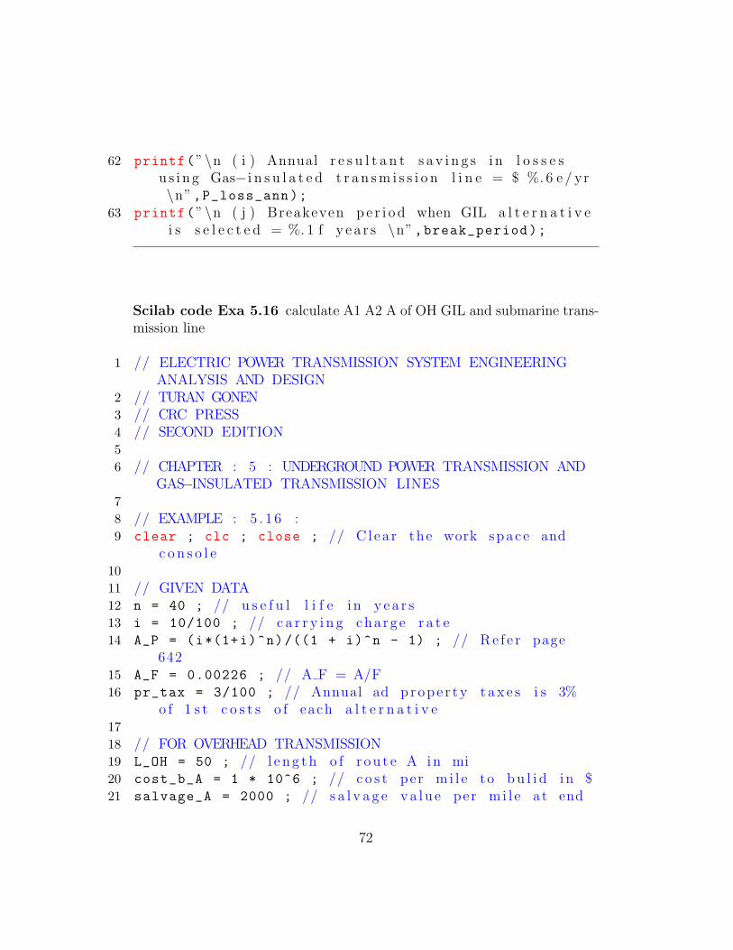
62 printf(”\n ( i ) Annual r e s u l t a n t s a v i n g s i n l o s s e su s i n g Gas− i n s u l a t e d t r a n s m i s s i o n l i n e = $ %. 6 e / yr\n”,P_loss_ann);

63 printf(”\n ( j ) Breakeven p e r i o d when GIL a l t e r n a t i v ei s s e l e c t e d = %. 1 f y e a r s \n”,break_period);

Scilab code Exa 5.16 calculate A1 A2 A of OH GIL and submarine trans-mission line




c o n s o l e1011 // GIVEN DATA12 n = 40 ; // u s e f u l l i f e i n y e a r s13 i = 10/100 ; // c a r r y i n g cha rge r a t e14 A_P = (i*(1+i)^n)/((1 + i)^n - 1) ; // Re f e r page

64215 A_F = 0.00226 ; // A F = A/F16 pr_tax = 3/100 ; // Annual ad p r o p e r t y t a x e s i s 3%

o f 1 s t c o s t s o f each a l t e r n a t i v e1718 // FOR OVERHEAD TRANSMISSION19 L_OH = 50 ; // l e n g t h o f r o u t e A i n mi20 cost_b_A = 1 * 10^6 ; // c o s t per m i l e to b u l i d i n $21 salvage_A = 2000 ; // s a l v a g e v a l u e per m i l e at end

72

o f 40 y e a r s22 cost_mait_OH = 500 ; // c o s t i n $ per m i l e to

ma inta in2324 // SUBMARINE TRANSMISSION LINE25 L_S = 30 ; // l e n g t h o f r o u t e B i n mi26 cost_b_B = 4*10^6 ; // c o s t per m i l e to b u l i d i n $27 salvage_B = 6000 ; // s a l v a g e v a l u e per m i l e at end

o f 40 y e a r s28 cost_mait_S = 1500 ; // c o s t i n $ per m i l e to

ma inta in2930 // GIL TRANSMISSION31 L_GIL = 20 ; // l e n g t h o f r o u t e C i n mi32 cost_b_C = 7.6*10^6 ; // c o s t per m i l e to b u l i d i n $33 salvage_C = 1000 ; // s a l v a g e v a l u e per m i l e at end

o f 40 y e a r s34 cost_mait_GIL = 200 ; // c o s t i n $ per m i l e to

ma inta in35 savings = 17.5*10^6 ; // r e l a t i v e s a v i n g s i n power

l o s s per yea r i n $363738 // CALCULATIONS39 n = 25 ; // u s e f u l l i f e i n y e a r s40 i = 20/100 ; // c a r r y i n g cha rge r a t e41 p = ((1 + i)^n - 1)/(i*(1+i)^n) ; // p = P/A42 // FOR OVERHEAD TRANSMISSION43 P_OH = cost_b_A * L_OH ; // f i r s t c o s t o f 500 kV OH

l i n e i n $44 F_OH = salvage_A * L_OH ; // Est imated s a l v a g e v a l u e

i n $45 A_1 = P_OH * A_P - F_OH * A_F ; // Annual e q u i v a l e n t

c o s t o f c a p i t a l i n $46 A_2 = P_OH * pr_tax + cost_mait_OH * L_OH ; //

annual e q u i v a l e n t c o s t o f tax and ma in ta inance i n$

47 A = A_1 + A_2 ; // t o t a l annua l e q u i c o s t o f OH l i n e

73

i n $4849 // SUBMARINE TRANSMISSION LINE50 P_S = cost_b_B * L_S ; // f i r s t c o s t o f 500 kV OH

l i n e i n $51 F_S = salvage_B * L_S ; // Est imated s a l v a g e v a l u e

i n $52 B_1 = P_S * A_P - F_S * A_F ; // Annual e q u i v a l e n t

c o s t o f c a p i t a l i n $53 B_2 = P_S * pr_tax + cost_mait_S * L_S ; // annual

e q u i v a l e n t c o s t o f tax and ma in ta inance i n $54 B = B_1 + B_2 ; // t o t a l annua l e q u i c o s t o f OH l i n e

i n $5556 // GIL TRANSMISSION57 P_GIL = cost_b_C * L_GIL ; // f i r s t c o s t o f 500 kV

OH l i n e i n $58 F_GIL = salvage_C * L_GIL ; // Est imated s a l v a g e

v a l u e i n $59 C_1 = P_GIL * A_P - F_GIL * A_F ; // Annual

e q u i v a l e n t c o s t o f c a p i t a l i n $60 C_2 = P_GIL * pr_tax + cost_mait_GIL * L_GIL ; //

annual e q u i v a l e n t c o s t o f tax and ma in ta inance i n$

61 C = C_1 + C_2 ; // t o t a l annua l e q u i c o s t o f OH l i n ei n $

62 A_net = C - savings ; // Tota l net annual e q u i c o s to f GIL


66 printf(”\n OVERHEAD TRANSMISSION LINE : \n”) ;

67 printf(”\n Annual e q u i v a l e n t c o s t o f c a p i t a li n v e s t e d i n l i n e , A 1 = $ %d \n”,A_1) ;

68 printf(”\n Annual e q u i v a l e n t c o s t o f Tax andma in ta inance , A 2 = $ %d \n”,A_2) ;

69 printf(”\n Tota l annual e q u i v a l e n t c o s t o f OHt r a n s m i s s i o n , A = $ %d \n”,A) ;

74

70 printf(”\n \n SUBMARINE TRANSMISSION LINE : \n”) ;

71 printf(”\n Annual e q u i v a l e n t c o s t o f c a p i t a li n v e s t e d i n l i n e , A 1 = $ %d \n”,B_1) ;

72 printf(”\n Annual e q u i v a l e n t c o s t o f Tax andma in ta inance , A 2 = $ %d \n”,B_2) ;

73 printf(”\n Tota l annual e q u i v a l e n t c o s t o fSubmarine power t r a n s m i s s i o n , A = $ %d \n”,B) ;

74 printf(”\n \n GIL TRANSMISSION LINE : \n”) ;

75 printf(”\n Annual e q u i v a l e n t c o s t o f c a p i t a li n v e s t e d i n l i n e , A 1 = $ %d \n”,C_1) ;

76 printf(”\n Annual e q u i v a l e n t c o s t o f Tax andma in ta inance , A 2 = $ %d \n”,C_2) ;

77 printf(”\n Tota l annual e q u i v a l e n t c o s t o fSubmarine power t r a n s m i s s i o n , A = $ %d \n”,C) ;

78 printf(”\n Tota l net e q u i v a l e n t c o s t o f GILt r a n s m i s s i o n = $ %d \n”,A_net) ;

79 printf(”\n \n The r e s u l t shows use o f GIL i s theb e s t c h o i c e \n”) ;

80 printf(”\n The next b e s t a l t e r n a t i v e i s Overheadt r a n s m i s s i o n l i n e \n”) ;

75

Chapter 6

DIRECT CURRENT POWERTRANSMISSION

Scilab code Exa 6.1 determine Vd Id ratio of dc to ac insulation level


2 // TURAN GONEN3 // CRC PRESS4 // SECOND EDITION56 // CHAPTER : 6 : DIRECT CURRENT POWER TRANSMISSION78 // EXAMPLE : 6 . 1 :9 clear ; clc ; close ; // C l ea r the work space and

c o n s o l e1011 // GIVEN DATA12 K_1 = 2.5 ; // Facto r13 K_2 = 1.7 ; // Facto r1415 // CALCULATIONS16 // For c a s e ( b )17 I_d = poly(0, ’ I d ’ ) ; // s i n c e P l o s s ( dc ) = P l o s s (

76

ac )18 I_L = poly(0, ’ I L ’ ) ; // i . e 2∗ I d ˆ2∗R dc = 3∗ I L ˆ2∗

R ac19 I_d = sqrt (3/2)*I_L ; // I g n o r i n g s k i n e f f e c t s R dc

= R ac20 I_d1 = 1.225* I_L ; // Re f e r Equ 6 . 2 32122 // For c a s e ( a )23 V_d = poly(0, ’ V d ’ ) ; // D e f i n i n g a p l oynomia l V d24 E_p = poly(0, ’ E p ’ ) ; // s i n c e P dc = P ac ( or ) V d∗

I d = 3∗E p∗ I L25 V_d = 2.45* E_p ; // Re f e r Equ 6 . 2 52627 // For c a s e ( c )28 ins_lvl = (K_2*(V_d /2))/(K_1*E_p) ; // Rat io o f dc

i n s u l a t i o n l e v e l to ac i n s u l a t i o n l e v e l29 ins_lvl_1 = (K_2 *2.45/2)/K_1 ; // s i m p l i f y i n g above

equ30 dc_i = poly(0, ’ d c i ’ ) ; // d c i = dc i n s u l a t i o n

l e v e l31 ac_i = poly(0, ’ a c i ’ ) ; // a c i = ac i n s u l a t i o n

l e v e l32 dc_i = ins_lvl_1 * ac_i ;


36 printf(”\n ( a ) Line−to− l i n e dc v o l t a g e o f V d i nterms o f l i n e −to−n e u t r a l v o l t a g e E p , V d = \n”); disp(V_d) ;

37 printf(”\n ( b ) The dc l i n e c u r r e n t I d i n terms o fac l i n e c u r r e n t I L , I d = \n”); disp(I_d1) ;

38 printf(”\n ( c ) Rat io o f dc i n s u l a t i o n l e v e l to aci n s u l a t i o n l e v e l = \n”) ; disp(dc_i/ac_i) ;

39 printf(”\n ( or ) dc i n s u l a t i o n l e v e l = \n”) ; disp(

dc_i) ;

77

Scilab code Exa 6.2 determine Vd ratio of Pdc to Pac and Ploss dc toPloss ac


2 // TURAN GONEN3 // CRC PRESS4 // SECOND EDITION56 // CHAPTER : 6 : DIRECT CURRENT POWER TRANSMISSION78 // EXAMPLE : 6 . 2 :9 clear ; clc ; close ; // C l ea r the work space and

c o n s o l e1011 // GIVEN DATA12 K = 3 ; // f a c t o r1314 // CALCULATIONS15 // For c a s e ( a )16 V_d = poly(0, ’ V d ’ ) ; // d e f i n i n g a po lynomia l17 E_p = poly(0, ’ E p ’ ) ;

18 V_d = K*2*E_p ; // From equ 6 . 1 81920 // For c a s e ( b )21 P_dc = poly(0, ’ P dc ’ ) ;

22 P_ac = poly(0, ’ P ac ’ ) ;

23 P_dc = 2*P_ac ;

2425 // For c a s e ( c )26 P_ld = poly(0, ’ P ld ’ ) ; // P l o s s ( dc )27 P_la = poly(0, ’ P l a ’ ) ; // P l o s s ( ac )28 P_ld = (2/3)*P_la ;

29

78


32 printf(”\n ( a ) Maximum o p e r a t i n g V d i n terms o fv o l t a g e E p , V d = \n”) ; disp(V_d) ;

33 printf(”\n ( b ) Maximum power t r a n s m i s s i o n c a p a b i l i t yr a t i o , i . e , r a t i o o f P dc to P ac , P dc / P ac = \n

”) ; disp(P_dc/P_ac) ;

34 printf(”\n ( or ) P dc = \n”) ; disp(P_dc) ;

35 printf(”\n ( c ) Rat io o f t o t a l I ˆ2∗R l o s s e s , i . e ,Rat io o f P l o s s ( dc ) to P l o s s ( ac ) , which accompanymaximum power f l o w = \n”) ; disp(P_ld/P_la) ;

36 printf(”\n ( or ) P l o s s ( dc ) = \n”) ; disp(P_ld) ;

Scilab code Exa 6.3 calculate KVA rating Wye side KV rating


2 // TURAN GONEN3 // CRC PRESS4 // SECOND EDITION56 // CHAPTER : 6 : DIRECT−CURRENT POWER TRANSMISSION78 // EXAMPLE : 6 . 3 :9 clear ; clc ; close ; // C l ea r the work space and

c o n s o l e1011 // GIVEN DATA12 V_d0 = 125 ; // v o l t a g e r a t i n g o f b r i d g e r e c t i f i e r

i n kV13 V_dr0 = V_d0 ; // Max c o n t i n u o s no−l o ad d i r e c t

v o l t a g e i n kV14 I = 1600 ; // c u r r e n t r a t i n g o f b r i d g e r e c t i f i e r i n

A15 I_d = I ; // Max c o n t i n u o u s c u r r e n t i n A

79

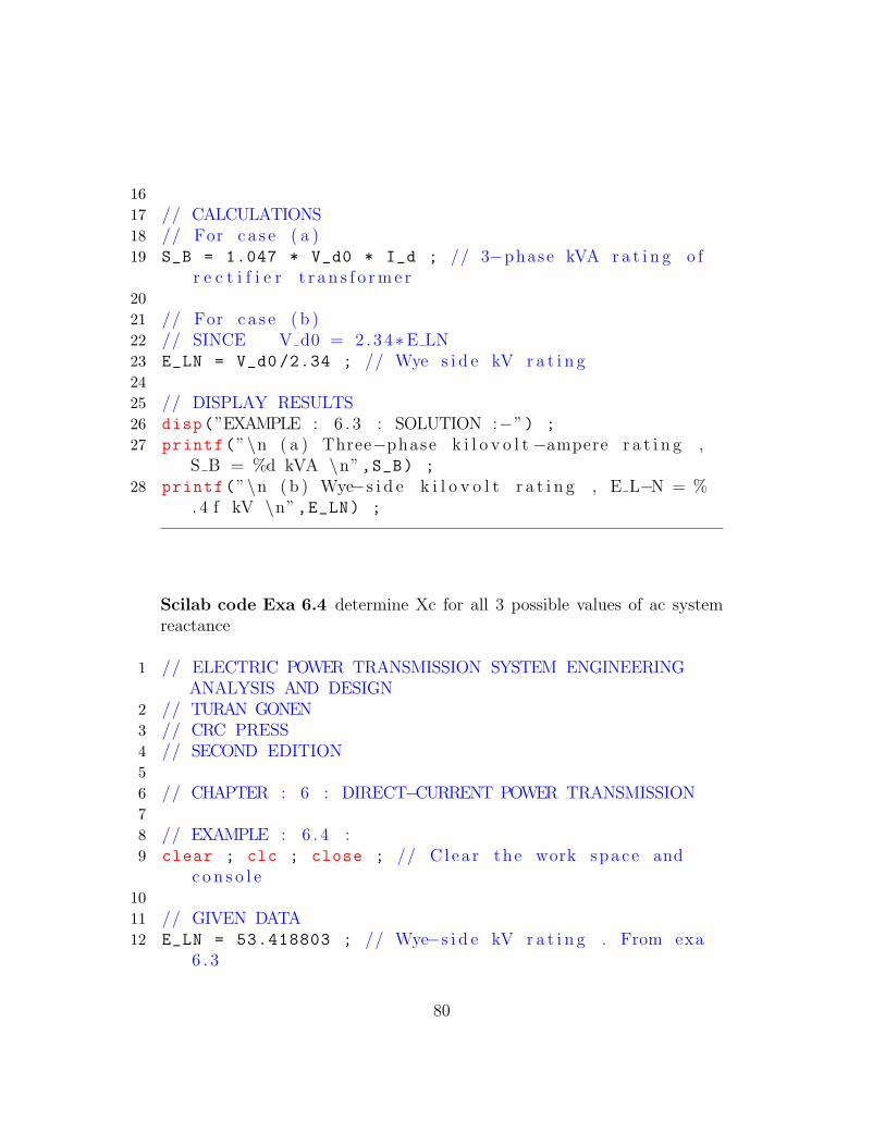
1617 // CALCULATIONS18 // For c a s e ( a )19 S_B = 1.047 * V_d0 * I_d ; // 3−phase kVA r a t i n g o f

r e c t i f i e r t r a n s f o r m e r2021 // For c a s e ( b )22 // SINCE V d0 = 2 . 3 4∗E LN23 E_LN = V_d0 /2.34 ; // Wye s i d e kV r a t i n g2425 // DISPLAY RESULTS26 disp(”EXAMPLE : 6 . 3 : SOLUTION :−”) ;

27 printf(”\n ( a ) Three−phase k i l o v o l t −ampere r a t i n g ,S B = %d kVA \n”,S_B) ;

28 printf(”\n ( b ) Wye−s i d e k i l o v o l t r a t i n g , E L−N = %. 4 f kV \n”,E_LN) ;

Scilab code Exa 6.4 determine Xc for all 3 possible values of ac systemreactance



c o n s o l e1011 // GIVEN DATA12 E_LN = 53.418803 ; // Wye−s i d e kV r a t i n g . From exa

6 . 3

80

13 I = 1600 ; // c u r r e n t r a t i n g o f b r i d g e r e c t i f i e r i nA

14 I_d = I ; // Max c o n t i n u o u s c u r r e n t i n A15 X_tr = 0.10 ; // impedance o f r e c t i f i e r t r a n s f o r m e r

i n pu1617 // For c a s e ( a )18 sc_MVA1 = 4000 ; // shor t−ck t MVA1920 // For c a s e ( b )21 sc_MVA2 = 2500 ; // shor t−ck t MVA2223 // For c a s e ( c )24 sc_MVA3 = 1000 ; // shor t−ck t MVA2526 // CALCULATIONS27 nom_kV = sqrt (3) * E_LN ; // Nominal kV L−L28 I_1ph = sqrt (2/3) * I_d ; // rms v a l u e o f wye−s i d e

phase c u r r e n t29 E_LN1 = E_LN * 10^3 ; // Wye−s i d e r a t i n g i n kV30 X_B = (E_LN1/I_1ph) ; // A s s o c i a t e d r e a c t a n c e base

i n3132 // For c a s e ( a )33 X_sys1 = nom_kV ^2/ sc_MVA1 ; // system r e a c t a n c e i n

34 X_tra = X_tr * X_B ; // Reactance o f r e c t i f i e rt r a n s f o r m e r

35 X_C = X_sys1 + X_tra ; // Commutating r e a c t a n c e i n

3637 // For c a s e ( b )38 X_sys2 = nom_kV ^2/ sc_MVA2 ; // system r e a c t a n c e i n

39 X_C2 = X_sys2 + X_tra ; // Commutating r e a c t a n c e i n

4041 // For c a s e ( b ) When b r e a k e r 1 & 2 a r e open

81

42 X_sys3 = nom_kV ^2/ sc_MVA3 ; // system r e a c t a n c e i n

43 X_C3 = X_sys3 + X_tra ; // Commutating r e a c t a n c e i n


47 printf(”\n ( a ) Commutating r e a c t a n c e When a l l t h r e eb r e a k e r s a r e c l o s e d , X C = %. 4 f \n”,X_C) ;

48 printf(”\n ( b ) Commutating r e a c t a n c e When b r e a k e r 1i s open , X C = %. 4 f \n”,X_C2) ;

49 printf(”\n ( c ) Commutating r e a c t a n c e When b r e a k e r s 1and 2 a r e open , X C = %. 4 f \n”,X_C3) ;

Scilab code Exa 6.5 calculate u Vdr pf Qr



c o n s o l e1011 // GIVEN DATA12 X_C = 6.2292017 ; // commutating r e a c t a n c e when a l l

3 b r e a k e r s a r e c l o s e d13 E_LN = 53.418803 * 10^3 ; // Wye−s i d e v o l t r a t i n g14 V_d0 = 125 * 10^3 ; // v o l t a g e r a t i n g o f b r i d g e

r e c t i f i e r i n V15 V_dr0 = V_d0 ; // Max c o n t i n u o s no−l o ad d i r e c t

82

v o l t a g e i n V16 I = 1600 ; // c u r r e n t r a t i n g o f b r i d g e r e c t i f i e r i n

A17 I_d = I ; // Max c o n t i n u o u s c u r r e n t18 nom_kV = sqrt (3) * E_LN ; // Nominal kV L−L19 X_tr = 0.10 ; // impedance o f r e c t i f i e r t r a n s f o r m e r

i n pu20 alpha = 0 ; // d e l a y a n g l e = 0 d e g r e e2122 // CALCULATIONS23 // For c a s e ( a )24 E_m = sqrt (2) * E_LN ;

25 u = acosd(1 - (2*X_C*I_d)/(sqrt (3)*E_m)); // o v e r l a pa n g l e when d e l a y a n g l e = 0 d e g r e e

2627 // For c a s e ( b )28 R_C = (3/%pi) * X_C ; // Equ commutation r e s i s t a n c e

per phase29 V_d = V_d0 * cosd(alpha) - R_C * I_d ; // dc v o l t a g e

o f r e c t i f i e r i n V3031 // For c a s e ( c )32 cos_theta = V_d/V_d0 ; // Di sp lacement or power

f a c t o r o f r e c t i f i e r3334 // For c a s e ( d )35 Q_r = V_d * I_d * tand( acosd(cos_theta) ) ; //

magne t i z i ng var I /P3637 // DISPLAY RESULTS38 disp(”EXAMPLE : 6 . 5 : SOLUTION :−”) ;

39 printf(”\n ( a ) Over lap a n g l e u o f r e c t i f i e r , u = %. 2f d e g r e e \n”,u) ;

40 printf(”\n ( b ) The dc v o l t a g e V dr o f r e c t i f i e r ,V dr = %. 2 f V \n”,V_d) ;

41 printf(”\n ( c ) Di sp lacement f a c t o r o f r e c t i f i e r ,c o s = %. 3 f \n”,cos_theta) ;

42 printf(”\n and = %. 1 f d e g r e e \n ”,acosd(

83

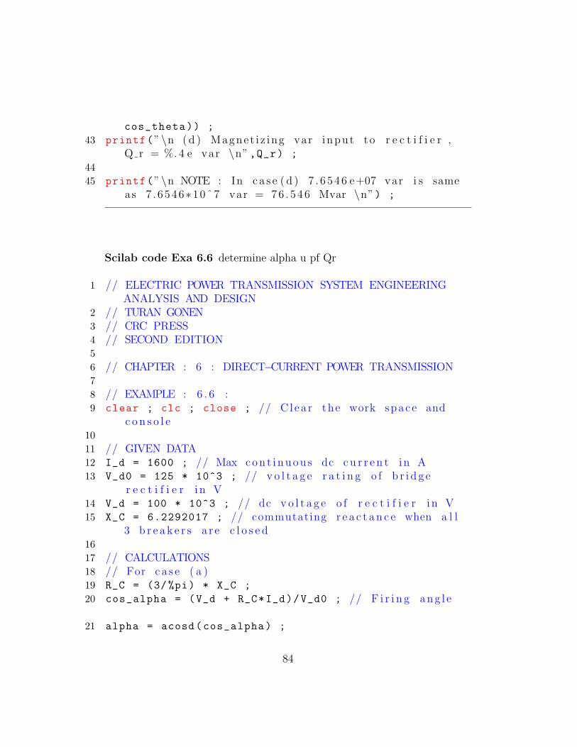
cos_theta)) ;

43 printf(”\n ( d ) Magnet i z ing var input to r e c t i f i e r ,Q r = %. 4 e var \n”,Q_r) ;

4445 printf(”\n NOTE : In c a s e ( d ) 7 . 6 5 4 6 e+07 var i s same

as 7 . 6546∗10ˆ7 var = 7 6 . 5 4 6 Mvar \n”) ;

Scilab code Exa 6.6 determine alpha u pf Qr



c o n s o l e1011 // GIVEN DATA12 I_d = 1600 ; // Max c o n t i n u o u s dc c u r r e n t i n A13 V_d0 = 125 * 10^3 ; // v o l t a g e r a t i n g o f b r i d g e

r e c t i f i e r i n V14 V_d = 100 * 10^3 ; // dc v o l t a g e o f r e c t i f i e r i n V15 X_C = 6.2292017 ; // commutating r e a c t a n c e when a l l

3 b r e a k e r s a r e c l o s e d1617 // CALCULATIONS18 // For c a s e ( a )19 R_C = (3/%pi) * X_C ;

20 cos_alpha = (V_d + R_C*I_d)/V_d0 ; // F i r i n g a n g l e

21 alpha = acosd(cos_alpha) ;

84

2223 // For c a s e ( b )24 // V d = ( 1 / 2 ) ∗V d0 ∗ ( c o s a l p h a + c o s d e l t a )25 cos_delta = (2 * V_d/V_d0) - cos_alpha ;

26 delta = acosd(cos_delta) ;

27 u = delta - alpha ; // Over lap a n g l e u i n d e g r e e2829 // For c a s e ( c )30 cos_theta = V_d/V_d0 ; // power f a c t o r31 theta = acosd(cos_theta) ;

3233 // For c a s e ( d )34 Q_r = V_d * I_d * tand(theta) ; // magne t i z i ng var I

/P3536 // DISPLAY RESULTS37 disp(”EXAMPLE : 6 . 6 : SOLUTION :−”) ;

38 printf(”\n ( a ) F i r i n g a n g l e o f r e c t i f i e r , = %. 2 f d e g r e e \n”,alpha) ;

39 printf(”\n ( b ) Over lap a n g l e u o f r e c t i f i e r , u = %. 2f d e g r e e \n”,u) ;

40 printf(”\n ( c ) Power f a c t o r , c o s = %. 2 f \n”,cos_theta) ;

41 printf(”\n and = %. 2 f d e g r e e \n ”,theta) ;

42 printf(”\n ( d ) Magnet i z ing var input , Q r = %. 2 evar \n”,Q_r) ;

Scilab code Exa 6.7 determine u mode Id or Vdr


2 // TURAN GONEN3 // CRC PRESS4 // SECOND EDITION5

85

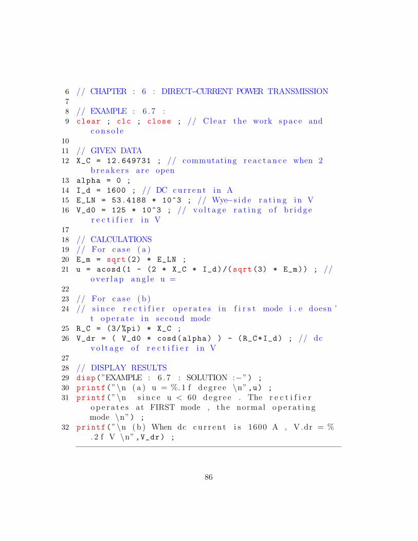
6 // CHAPTER : 6 : DIRECT−CURRENT POWER TRANSMISSION78 // EXAMPLE : 6 . 7 :9 clear ; clc ; close ; // C l ea r the work space and

c o n s o l e1011 // GIVEN DATA12 X_C = 12.649731 ; // commutating r e a c t a n c e when 2

b r e a k e r s a r e open13 alpha = 0 ;

14 I_d = 1600 ; // DC c u r r e n t i n A15 E_LN = 53.4188 * 10^3 ; // Wye−s i d e r a t i n g i n V16 V_d0 = 125 * 10^3 ; // v o l t a g e r a t i n g o f b r i d g e

r e c t i f i e r i n V1718 // CALCULATIONS19 // For c a s e ( a )20 E_m = sqrt (2) * E_LN ;

21 u = acosd(1 - (2 * X_C * I_d)/(sqrt (3) * E_m)) ; //o v e r l a p a n g l e u =

2223 // For c a s e ( b )24 // s i n c e r e c t i f i e r o p e r a t e s i n f i r s t mode i . e doesn ’

t o p e r a t e i n second mode25 R_C = (3/%pi) * X_C ;

26 V_dr = ( V_d0 * cosd(alpha) ) - (R_C*I_d) ; // dcv o l t a g e o f r e c t i f i e r i n V


30 printf(”\n ( a ) u = %. 1 f d e g r e e \n”,u) ;

31 printf(”\n s i n c e u < 60 d e g r e e . The r e c t i f i e ro p e r a t e s at FIRST mode , the normal o p e r a t i n gmode \n”) ;

32 printf(”\n ( b ) When dc c u r r e n t i s 1600 A , V dr = %. 2 f V \n”,V_dr) ;

86

Scilab code Exa 6.10 determine Vd0 E u pf Qr No of bucks


2 // TURAN GONEN3 // CRC PRESS4 // SECOND EDITION56 // CHAPTER : 6 : DIRECT−CURRENT POWER TRANSMISSION78 // EXAMPLE : 6 . 1 0 :9 clear ; clc ; close ; // C l ea r the work space and

c o n s o l e1011 // GIVEN DATA12 X_C = 6.2292 ; // commutating r e a c t a n c e when a l l 3

b r e a k e r s a r e c l o s e d13 I_db = 1600 ; // dc c u r r e n t base i n A14 V_db = 125 * 10^3 ; // dc v o l t a g e base i n V15 I_d = I_db ; // Max c o n t i n u o u s c u r r e n t i n A16 V_d = 100 * 10^3 ; // dc v o l t a g e i n V17 alpha = 0 ; // F i r i n g a n g l e = 0 d e g r e e1819 // CALCULATIONS20 // For c a s e ( a )21 R_c = (3/%pi) * X_C ;

22 R_cb = V_db/I_db ; // R e s i s t a n c e base i n23 V_d_pu = V_d/V_db ; // per u n i t v o l t a g e24 I_d_pu = I_d/I_db ; // per u n i t c u r r e n t25 R_c_pu = R_c/R_cb ; // per u n i t26 E_pu = (V_d_pu + R_c_pu * I_d_pu)/cosd(alpha) ; //

Open ckt dc v o l t a g e i n pu27 V_d0 = E_pu * V_db ; // Open ckt dc v o l t a g e i n V28

87

29 // For c a s e ( b )30 E = V_d0 /2.34; // Open ckt ac v o l t a g e on wye s i d e o f

t r a n s f o r m e r i n V3132 // For c a s e ( c )33 E_1LN = 92.95 * 10^3 ; // v o l t a g e i n V34 E_1B = E_1LN ;

35 E_LN = 53.44 * 10^3 ; // v o l t a g e i n V36 a = E_1LN/E_LN ;

37 n = a ; // when LTC on n e u t r a l38 X_c_pu = 2 * R_c_pu ;

39 E_1_pu = E_1LN / E_1B ; // per u n i t v o l t a g e40 cos_delta = cosd(alpha) - ( (X_c_pu * I_d_pu)/( (a/n

) *E_1_pu) ) ;

41 delta = acosd(cos_delta) ;

42 u = delta - alpha ;

4344 // For c a s e ( d )45 cos_theta = V_d/V_d0 ; // p f o f r e c t i f i e r46 theta = acosd(cos_theta) ;

4748 // For c a s e ( e )49 Q_r = V_d*I_d*tand(theta) ; // magne t i z i ng var I /P5051 // For c a s e ( f )52 d_V = E_LN - E ; // n e c e s s a r y change i n v o l t a g e i n V53 p_E_LN = 0.00625 * E_LN ; // one buck s t e p can

change i n V/ s t e p54 no_buck = d_V / p_E_LN ; // No . o f s t e p s o f buck5556 // DISPLAY RESULTS57 disp(”EXAMPLE : 6 . 1 0 : SOLUTION :−”) ;

58 printf(”\n ( a ) Open c i r c u i t dc Vo l tage , V d0 = %. 2 fV \n”,V_d0);

59 printf(”\n ( b ) Open c i r c u i t ac v o l t a g e on wye s i d eo f t r a n s f o r m e r , E = %. 2 f V \n”,E);

60 printf(”\n ( c ) Over lap a n g l e , u = %. 2 f d e g r e e \n”,u)

88

61 printf(”\n ( d ) Power f a c t o r , c o s = %. 3 f \n”,cos_theta);

62 printf(”\n and = %. 2 f d e g r e e \n ”,theta);63 printf(”\n ( e ) Magnet i z ing var input to r e c t i f i e r ,

Q r = %. 4 e var \n”,Q_r);64 printf(”\n ( f ) Number o f 0 . 6 2 5 p e r c e n t s t e p s o f buck

r e q u i r e d , No . o f buck = %. f s t e p s \n”,no_buck);

89

Chapter 7

TRANSIENTOVERVOLTAGES ANDINSULATIONCOORDINATION

Scilab code Exa 7.1 determine surge Power surge current


2 // TURAN GONEN3 // CRC PRESS4 // SECOND EDITION56 // CHAPTER : 7 : TRANSIENT OVERVOLTAGES AND

INSULATION COORDINATION78 // EXAMPLE : 7 . 1 :9 clear ; clc ; close ; // C l ea r the work space and

c o n s o l e1011 // GIVEN DATA12 V = 1000 ; // s u r g e v o l t a g e i n kV

90

13 Z_c = 500 ; // s u r g e impedance i n1415 // CALCULATIONS16 // For c a s e ( a )17 P = V^2/Z_c ; // Tota l s u r g e power i n MW1819 // For c a s e ( b )20 V1 = V*10^3 ; // s u r g e v o l t a g e i n V21 i = V1/Z_c ;// s u r g e c u r r e n t i n A2223 // DISPLAY RESULTS24 disp(”EXAMPLE : 7 . 1 : SOLUTION :−”) ;

25 printf(”\n ( a ) Tota l s u r g e power i n l i n e , P = %d MW\n”,P) ;

26 printf(”\n ( b ) Surge c u r r e n t i n l i n e , i = %d A \n”,i) ;

Scilab code Exa 7.2 determine surge Power surge current




c o n s o l e1011 // GIVEN DATA12 V = 1000 ; // s u r g e v o l t a g e i n kV13 Z_c = 50 ; // s u r g e impedance i n

91

1415 // CALCULATIONS16 // For c a s e ( a )17 P = V^2/Z_c ; // Tota l s u r g e power i n MW1819 // For c a s e ( b )20 V1 = V*10^3 ; // s u r g e v o l t a g e i n V21 i = V1/Z_c ;// s u r g e c u r r e n t i n A2223 // DISPLAY RESULTS24 disp(”EXAMPLE : 7 . 1 : SOLUTION :−”) ;

25 printf(”\n ( a ) Tota l s u r g e power i n l i n e , P = %d MW\n”,P) ;

26 printf(”\n ( b ) Surge c u r r e n t i n l i n e , i = %d A \n”,i) ;

Scilab code Exa 7.4 determine Crv Cri vb v Crfv ib i Crfi




c o n s o l e1011 // GIVEN DATA12 R = 500 ; // R e s i s t a n c e i n13 Z_c = 400 ; // c h a r a c t e r i s t i c impedance i n14 v_f = 5000 ; // Forward t r a v e l l i n g v o l t a g e wave i n V

92

15 i_f = 12.5 ; // Forward t r a v e l l i n g c u r r e n t wave i n A1617 // CALCULATIONS18 // For c a s e ( a )19 r_v = (R - Z_c)/(R + Z_c) ; // R e f l e c t i o n

c o e f f i c i e n t o f v o l t a g e wave2021 // For c a s e ( b )22 r_i = -(R - Z_c)/(R + Z_c) ; // R e f l e c t i o n

c o e f f i c i e n t o f c u r r e n t wave2324 // For c a s e ( c )25 v_b = r_v * v_f ; // Backward−t r a v e l l i n g v o l t a g e

wave i n V2627 // For c a s e ( d )28 v = v_f + v_b ; // Vo l tage at end o f l i n e i n V29 v1 = (2 * R/(R + Z_c)) * v_f ; // ( or ) Vo l tage at

end o f l i n e i n V3031 // For c a s e ( e )32 t1 = (2 * R/(R + Z_c)) ; // R e f r a c t i o n c o e f f i c i e n t

o f v o l t a g e wave3334 // For c a s e ( f )35 i_b = -( v_b/Z_c ) ; // backward−t r a v e l l i n g c u r r e n t

wave i n A36 i_b1 = -r_v * i_f ; // ( or ) backward−t r a v e l l i n g

c u r r e n t wave i n A373839 // For c a s e ( g )40 i = v/R ; // Current f l o w i n g through r e s i s t o r i n A4142 // For c a s e ( h )43 t2 = (2 * Z_c/(R + Z_c)) ; // R e f r a c t i o n c o e f f i c i e n t

o f c u r r e n t wave44

93


47 printf(”\n ( a ) R e f l e c t i o n c o e f f i c i e n t o f v o l t a g ewave , = %. 4 f \n”,r_v) ;

48 printf(”\n ( b ) R e f l e c t i o n c o e f f i c i e n t o f c u r r e n twave , = %. 4 f \n”,r_i) ;

49 printf(”\n ( c ) Backward−t r a v e l l i n g v o l t a g e wave ,v b = %. 3 f V \n”,v_b) ;

50 printf(”\n ( d ) Vo l tage at end o f l i n e , v = %. 3 f V \n”,v) ;

51 printf(”\n From a l t e r n a t i v e method ”)52 printf(”\n Vo l tage at end o f l i n e , v = %. 3 f V \

n”,v) ;

53 printf(”\n ( e ) R e f r a c t i o n c o e f f i c i e n t o f v o l t a g ewave , = %. 4 f \n”,t1) ;

54 printf(”\n ( f ) Backward−t r a v e l l i n g c u r r e n t wave ,i b = %. 4 f A \n”,i_b) ;

55 printf(”\n ( g ) Current f l o w i n g through r e s i s t o r , i =%. 4 f A \n”,i) ;

56 printf(”\n ( h ) R e f r a c t i o n c o e f f i c i e n t o f c u r r e n twave , = %. 4 f \n”,t2) ;

Scilab code Exa 7.5 determine if Cr Crf v i vb ib plot of voltage andcurrent surges



INSULATION COORDINATION78 // EXAMPLE : 7 . 5 :

94


1011 // GIVEN DATA12 Z_c1 = 400 ; // Surge impedance o f l i n e i n13 Z_c2 = 40 ; // Surge impedance o f c a b l e i n14 v_f = 200 ; // Forward t r a v e l l i n g s u r g e v o l t a g e i n

kV1516 // CALCULATIONS17 // For c a s e ( a )18 v_f1 = v_f * 10^3 ; // s u r g e v o l t a g e i n V19 i_f = v_f1/Z_c1 ; // Magnitude o f f o rward c u r r e n t

wave i n A2021 // For c a s e ( b )22 r = (Z_c2 - Z_c1)/(Z_c2 + Z_c1) ; // R e f l e c t i o n

c o e f f i c i e n t2324 // For c a s e ( c )25 t = 2 * Z_c2/(Z_c2 + Z_c1) ; // R e f r a c t i o n

c o e f f i c i e n t2627 // For c a s e ( d )28 v = t * v_f ; // Surge v o l t a g e t r a n s m i t t e d fo rward

i n t o c a b l e i n kV2930 // For c a s e ( e )31 v1 = v * 10^3 ; // Surge v o l t a g e t r a n s m i t t e d fo rward

i n t o c a b l e i n V32 I = v1/Z_c2 ; // Surge c u r r e n t t r a n s m i t t e d fo rward

i n t o c a b l e i n A3334 // For c a s e ( f )35 v_b = r * v_f ; // s u r g e v o l t a g e r e f l e c t e d back

a l ong overhead l i n e i n kV3637 // For c a s e ( g )

95

38 i_b = -r * i_f ; // s u r g e c u r r e n t r e f l e c t e d backa l ong overhead l i n e i n A

3940 // For c a s e ( h )41 // A r b i t r a r y v a l u e s a r e taken i n graph . Only f o r

r e f e r e n c e not f o r s c a l e42 T = 0:0.1:300 ;

4344 for i = 1:int(length(T)/3) ; // p l o t t i n g Vo l tage

v a l u e s45 vo(i) = 3;

46 end

47 for i = int(length(T)/3):length(T)

48 vo(i) = 1 ;

49 end

50 for i = int(length(T))

51 vo(i) = 0 ;

52 end

535455 a=gca() ;

56 ylabel(”CURRENT SENDING ENDVOLTAGE ”) ;

57 b = newaxes () ; // c r e a t e s new a x i s58 b.y_location = ” r i g h t ” ; // P o s i t i o n o f a x i s59 ylabel (”RECEIVING END”) ; // L a b e l l i n g y−a x i s60 b.axes_visible = [” o f f ”,” o f f ”,” o f f ”] ;

61 e = newaxes () ;

62 e.y_location = ” middle ” ;

63 e.y_label.text = ”JUNCTION” ;

64 subplot (2,1,1) ;

65 plot2d(T,vo ,2, ’ 012 ’ , ’ ’ ,[0,0,310,6]) ;

6667 for i = 1:int(length(T)/3) ; // P l o t t i n g c u r r e n t

s u r g e s v a l u e68 io(i) = 1 ;

69 end

70 for i = int(length(T)/3):length(T)

96

71 io(i) = 3 ;

72 end

73 for i = int(length(T))

74 io(i) = 0 ;

75 end

767778 c=gca() ;

79 d = newaxes () ;

80 d.y_location = ” r i g h t ” ;

81 d.filled = ” o f f ” ;

82 f.y_location = ” middle ” ;

83 f.y_label.text = ”JUNCTION” ;

84 subplot (2,1,2) ;

85 plot2d(T,io ,5, ’ 012 ’ , ’ ’ ,[0,0,310,6]) ;


89 printf(”\n ( a ) Magnitude o f f o rward c u r r e n t wave ,i f = %d A \n”,i_f) ;

90 printf(”\n ( b ) R e f l e c t i o n c o e f f i c i e n t , = %. 4 f \n”,r) ;

91 printf(”\n ( c ) R e f r a c t i o n c o e f f i c i e n t , = %. 4 f \n”,t) ;

92 printf(”\n ( d ) Surge v o l t a g e t r a n s m i t t e d fo rwardi n t o c a b l e , v = %. 2 f kV \n”,v) ;

93 printf(”\n ( e ) Surge c u r r e n t t r a n s m i t t e d fo rwardi n t o c a b l e , i = %. f A \n”,I) ;

94 printf(”\n ( f ) Surge v o l t a g e r e f l e c t e d back a l ongthe OH l i n e , v b = %. 2 f kV \n”,v_b) ;

95 printf(”\n ( g ) Surge c u r r e n t r e f l e c t e d back a l ongthe OH l i n e , i b = %. f A \n”,i_b) ;

96 printf(”\n ( h ) Graph shows p l o t o f v o l t a g e & c u r r e n ts u r g e s a f t e r a r r i v a l a t the j u n c t i o n \n”) ;

97

Scilab code Exa 7.6 determine Crs Crr lattice diagram volatge plot of re-ceiving end voltage with time




c o n s o l e1011 // GIVEN DATA12 v = 1000 ; // i d e a l dc v o l t a g e s o u r c e i n V13 Z_s = 0 ; // i n t e r n a l impedance i n14 Z_c = 40 ; // c h a r a c t e r i s t i c impedance i n15 Z_r = 60 ; // Cable i s t e rm ina t ed i n 60 r e s i s t o r1617 // CALCULATIONS18 // For c a s e ( a )19 r_s = (Z_s - Z_c)/(Z_s + Z_c) ; // R e f l e c t i o n

c o e f f i c i e n t at s e n d i n g end2021 // For c a s e ( b )22 r_r = (Z_r - Z_c)/(Z_r + Z_c) ; // R e f l e c t i o n

c o e f f i c i e n t at r e c e i v i n g end2324 // For c a s e ( c )25 T = 0:0.001:10.6 ; // // p l o t t i n g v a l u e s26 for i = 1: length(T) ;

27 if(T(i) <=1)

28 x(i) = (1.2)*T(i) - 1 ;

29 elseif(T(i) >=1 & T(i) <=2)

30 x(i) = ( -1.2)*T(i) + 1.4 ;

98

31 elseif(T(i) >=2 & T(i) <=3)

32 x(i) = (1.2)*T(i)- 3.4 ;

33 elseif(T(i) >=3 & T(i) <=4)

34 x(i) = ( -1.2)*T(i) + 3.8 ;

35 elseif(T(i) >=4 & T(i) <=5)

36 x(i) = (1.2)*T(i)- 5.8 ;

37 elseif(T(i) >=5 & T(i) <=6)

38 x(i) = ( -1.2)*T(i) + 6.2 ;

39 elseif(T(i) >=6 & T(i) <=7)

40 x(i) = (1.2)*T(i)- 8.2 ;

41 elseif(T(i) >=7 & T(i) <=8)

42 x(i) = ( -1.2)*T(i) + 8.6 ;

43 elseif(T(i) >=8 & T(i) <=9)

44 x(i) = (1.2)*T(i)- 10.6 ;

45 elseif(T(i) >=9 & T(i) <=10)

46 x(i) = ( -1.2)*T(i) + 11 ;

47 elseif(T(i) >=10 & T(i) <=10.6)

48 x(i) = (1.2)*T(i) - 13 ;

49 end

50 end

5152 subplot (2,1,1) ; // P l o t t i n g two graph i n same

window53 plot2d(T,x,5, ’ 012 ’ , ’ ’ ,[0,-1,11,0.2]) ;

5455 a = gca() ;

56 xlabel(”TIME”) ;

57 ylabel(” s = −1 DISTANCEr = 0 . 2 ”) ;

58 xtitle(” Fig 7 . 6 ( c ) L a t t i c e diagram ”) ;

59 a.thickness = 2 ; // s e t s t h i c k n e s s o f p l o t60 xset( ’ t h i c k n e s s ’ ,2) ; // s e t s t h i c k n e s s o f axe s61 xstring(1,-1, ’T ’ ) ;

62 xstring(2,-1, ’ 2T ’ ) ;

63 xstring(3,-1, ’ 3T ’ ) ;

64 xstring(4,-1, ’ 4T ’ ) ;

65 xstring(5,-1, ’ 5T ’ ) ;

66 xstring(6,-1, ’ 6T ’ ) ;

99

67 xstring(7,-1, ’ 7T ’ ) ;

68 xstring(8,-1, ’ 8T ’ ) ;

69 xstring(9,-1, ’ 9T ’ ) ;

70 xstring (10,-1, ’ 10T ’ ) ;

71 xstring (0.1,0.1, ’ 0V ’ ) ;

72 xstring (2,0.1, ’ 1200V ’ ) ;

73 xstring (4,0.1, ’ 960V ’ ) ;

74 xstring (6,0.1, ’ 1008V ’ ) ;

75 xstring (8,0.1, ’ 9 9 8 . 4V ’ ) ;

76 xstring (1,-0.88, ’ 1000V ’ ) ;

77 xstring (3,-0.88, ’ 1000V ’ ) ;

78 xstring (5,-0.88, ’ 1000V ’ ) ;

79 xstring (7,-0.88, ’ 1000V ’ ) ;

80 xstring (9,-0.88, ’ 1000V ’ ) ;

8182 // For c a s e ( d )83 q1 = v ; // Re f e r Fig 7 . 1 1 i n t ex tbook84 q2 = r_r * v ;

85 q3 = r_s * r_r * v ;

86 q4 = r_s * r_r^2 * v ;

87 q5 = r_s^2 * r_r^2 * v ;

88 q6 = r_s^2 * r_r^3 * v ;

89 q7 = r_s^3 * r_r^3 * v ;

90 q8 = r_s^3 * r_r^4 * v ;

91 q9 = r_s^4 * r_r^4 * v ;

92 q10 = r_s^4 * r_r^5 * v ;

93 q11 = r_s^5 * r_r^5 * v ;

94 V_1 = v - q1 ;

95 V_2 = v - q3 ;

96 V_3 = v - q5 ;

97 V_4 = v - q7 ; // v o l t a g e at t = 6 . 5T & x = 0 . 2 5 l i nV o l t s

98 V_5 = v - q9 ;

99100 // For c a s e ( e )101 t = 0:0.001:9 ;

102103 for i= 1: length(t)

100

104 if(t(i) >=0 & t(i) <=1)

105 y(i) = V_1 ;

106 elseif(t(i) >=1 & t(i) <=3)

107 y(i) = V_2 ;

108 elseif(t(i) >=3 & t(i) <=5)

109 y(i)= V_3 ;

110 elseif(t(i) >=5 & t(i) <=7)

111 y(i)= V_4 ;

112 elseif(t(i) >=7 & t(i) <=9)

113 y(i)= V_5 ;

114 end

115 end

116 subplot (2,1,2) ;

117 a = gca() ;

118 a.thickness = 2 ; // s e t s t h i c k n e s s o f p l o t119 plot2d(t,y,2, ’ 012 ’ , ’ ’ ,[0 ,0,10,1300]) ;

120 a.x_label.text = ’TIME (T) ’ ; // l a b e l s x−a x i s121 a.y_label.text = ’RECEIVING−END VOLTAGE (V) ’ ; //

l a b e l s y−a x i s122 xtitle(” Fig 7 . 6 ( e ) . P l o t o f R e c e i v i n g end Vo l tage

v/ s Time”) ;

123 xset( ’ t h i c k n e s s ’ ,2); // s e t s t h i c k n e s s o f axe s124 xstring (1,0, ’ 1T ’ ) ; // naming p o i n t s125 xstring (3,0, ’ 3T ’ ) ;

126 xstring (5,0, ’ 5T ’ ) ;

127 xstring (7,0, ’ 7T ’ ) ;

128 xstring (1,1200, ’ 1200 V ’ ) ;

129 xstring (4,960, ’ 960 V ’ ) ;

130 xstring (6,1008, ’ 1008 V ’ ) ;

131 xstring (8,998.4, ’ 9 9 8 . 4 V ’ ) ;


136 printf(”\n ( a ) R e f l e c t i o n c o e f f i c i e n t at s e n d i n g end, s = %. f \n”,r_s) ;

137 printf(”\n ( b ) R e f l e c t i o n c o e f f i c i e n t at s e n d i n g end, r = %. 1 f \n”,r_r)

101

138 printf(”\n ( c ) The l a t t i c e diagram i s shown i n Fig7 . 6 ( c ) \n”) ;

139 printf(”\n ( d ) From Fig 7 . 6 ( c ) , the v o l t a g e v a l u ei s at t = 6 . 5T & x = 0 . 2 5 l i s = %. d V o l t s \n”,V_4) ;

140 printf(”\n ( e ) The p l o t o f the r e c e i v i n g −end v o l t a g ev/ s t ime i s shown i n Fig 7 . 6 ( e ) \n”) ;

102

Chapter 8

LIMITING FACTORS FOREXTRA HIGH ANDULTRAHIGH VOLTAGETRANSMISSION

Scilab code Exa 8.1 determine disruptive critical rms V0 and visual crit-ical rms Vv


2 // TURAN GONEN3 // CRC PRESS4 // SECOND EDITION56 // CHAPTER : 8 : LIMITING FACTORS FOR EXTRA−HIGH AND

ULTRAHIGH VOLTAGE TRANSMISSION78 // EXAMPLE : 8 . 1 :9 clear ; clc ; close ; // C l ea r the work space and

c o n s o l e1011 // GIVEN DATA

103

12 m_0 = 0.90 ; // I r r e g u l a r i t y f a c t o r13 p = 74 ; // Atmospher ic p r e s s u r e i n Hg14 t = 10 ; // t empera tu re i n d e g r e e c e l s i u s15 D = 550 ; // E q u i l a t e r a l s p a c i n g b/w c o n d u c t o r s i n

cm16 d = 3 ; // o v e r a l l d i amete r i n cm1718 // CALCULATIONS19 // For c a s e ( a )20 r = d/2 ;

21 delta = 3.9211 * p/( 273 + t ) ; // a i r d e n s i t yf a c t o r

22 V_0_ph = 21.1 * delta * m_0 * r * log(D/r) ; //d i s r u p t i v e c r i t i c a l rms l i n e v o l t a g e i n kV/ phase

23 V_0 = sqrt (3) * V_0_ph ; // d i s r u p t i v e c r i t i c a l rmsl i n e v o l t a g e i n kV

2425 // For c a s e ( b )26 m_v = m_0 ;

27 V_v_ph = 21.1* delta*m_v*r*(1 + (0.3/ sqrt(delta*r) ))

* log(D/r) ; // v i s u a l c r i t i c a l rms l i n e v o l t a g ei n kV/ phase

28 V_v = sqrt (3)*V_v_ph ; // v i s u a l c r i t i c a l rms l i n ev o l t a g e i n kV


32 printf(”\n ( a ) D i s r u p t i v e c r i t i c a l rms l i n e v o l t a g e, V 0 = %. 1 f kV \n”,V_0) ;

33 printf(”\n ( b ) V i s u a l c r i t i c a l rms l i n e v o l t a g e ,V v = %. 1 f kV \n”,V_v) ;

Scilab code Exa 8.2 determine total fair weather corona loss Pc


104

ANALYSIS AND DESIGN2 // TURAN GONEN3 // CRC PRESS4 // SECOND EDITION56 // CHAPTER : 8 : LIMITING FACTORS FOR EXTRA−HIGH AND

ULTRAHIGH VOLTAGE TRANSMISSION78 // EXAMPLE : 8 . 2 :9 clear ; clc ; close ; // C l ea r the work space and

c o n s o l e1011 // GIVEN DATA12 f = 60 ; // f r e q i n Hz13 d = 3 ; // o v e r a l l d i amete r i n cm14 D = 550 ; // E q u i l a t e r a l s p a c i n g b/w c o n d u c t o r s i n

cm15 V1 = 345 ; // o p e r a t i n g l i n e v o l t a g e i n kV16 V_0 = 172.4 ; // d i s r u p t i v e c r i t i c a l v o l t a g e i n kV17 L = 50 ; // l i n e l e n g t h i n mi18 p = 74 ; // Atmospher ic p r e s s u r e i n Hg19 t = 10 ; // t empera tu re i n d e g r e e c e l s i u s20 m_0 = 0.90 ; // I r r e g u l a r i t y f a c t o r2122 // CALCULATIONS23 r = d/2 ;

24 delta = 3.9211 * p/( 273 + t ) ; // a i r d e n s i t yf a c t o r

25 V_0 = 21.1 * delta * m_0 * r * log(D/r) ; //d i s r u p t i v e c r i t i c a l rms l i n e v o l t a g e i n kV/ phase

26 V =V1/sqrt (3) ; // Line to n e u t r a l o p e r a t i n g v o l t a g ei n kV

27 P_c = (390/ delta)*(f+25)*sqrt(r/D)*(V - V_0)^2 *

10^-5 ; // F a i r weather corona l o s s per phase i nkW/mi/ phase

28 P_cT = P_c * L ; // For t o t a l l i n e l e n g t h coronal o s s i n kW/ phase

29 T_P_c = 3 * P_cT ; // Tota l co rona l o s s o f l i n e i n

105

kW3031 // DISPLAY RESULTS32 disp(”EXAMPLE : 8 . 2 : SOLUTION :−”) ;

33 printf(”\n ( a ) Tota l f a i r weather co rona l o s s o f thel i n e , P c = %. 1 f kW \n”,T_P_c) ;

106

Chapter 9

SYMMETRICALCOMPONENTS AND FAULTANALYSIS

Scilab code Exa 9.1 determine symmetrical components for phase volt-ages


2 // TURAN GONEN3 // CRC PRESS4 // SECOND EDITION56 // CHAPTER : 9 : SYMMETRICAL COMPONENTS AND FAULT

ANALYSIS78 // EXAMPLE : 9 . 1 :9 clear ; clc ; close ; // C l ea r the work space and

c o n s o l e1011 // GIVEN DATA12 V_a = 7.3 * exp(%i *12.5* %pi /180) ; // Phase v o l t a g e

i n V

107

13 V_b = 0.4 * exp(%i*( -100)*%pi /180) ; // Phasev o l t a g e i n V

14 V_c = 4.4 * exp(%i*154* %pi /180) ; // Phase v o l t a g ei n V

15 a = 1 * exp(%i*120* %pi /180) ; // o p e r a t o r ’ a ’ bya p p l i c a t i o n o f symmet r i c a l components th e o r y to3− system . R e f e r s e c t i o n 9 . 3 f o r d e t a i l s

1617 // CALCULATIONS18 V_a0 = (1/3) * (V_a + V_b + V_c) ; // A n a l y s i s equ

i n V19 V_a1 = (1/3) * (V_a + a*V_b + a^2*V_c) ;

20 V_a2 = (1/3) * (V_a + a^2*V_b + a*V_c) ;

21 V_b0 = V_a0 ;

22 V_b1 = a^2 * V_a1 ;

23 V_b2 = a * V_a2 ;

24 V_c0 = V_a0 ;

25 V_c1 = a * V_a1 ;

26 V_c2 = a^2 * V_a2 ;


30 printf(”\n The symmet r i c a l components f o r the phasev o l t a g e s V a , V b & V c a r e \n”) ;

31 printf(”\n V a0 = %. 2 f<%. 1 f V \n”,abs(V_a0),atand(imag(V_a0),real(V_a0) )) ;



34 printf(”\n V b0 = %. 2 f<%. 1 f V \n”,abs(V_b0),atand(imag(V_b0),real(V_b0) )) ;



37 printf(”\n V c0 = %. 2 f<%. 1 f V \n”,abs(V_c0),atand(imag(V_c0),real(V_c0) )) ;

108



4041 printf(”\n NOTE : V b1 = 3.97 <−99.5 V & V c2 =

2.52 <−139.7 V r e s u l t o b t a i n e d i s same as t ex tbookanswer V b1 = 3.97 <260 .5 V & V c2 = 2.52 <220 .3 V\n”) ;

42 printf(”\n Changes i s due to a ˆ2 = 1<240 = 1<−120where 1 i s the magnitude & <240 i s the a n g l e i nd e g r e e \n”) ;

Scilab code Exa 9.2 determine complex power V012 I012




c o n s o l e1011 // GIVEN DATA12 V_abc = [0 ; 50 ; -50] ; // Phase v o l t a g e s o f a 3−

system i n V13 I_abc = [-5 ; 5*%i ; -5] ; // Phase c u r r e n t o f a 3−

system i n A1415 // CALCULATIONS

109

16 // For c a s e ( a )17 S_3ph = (V_abc)’ * conj(I_abc) ; // 3− complex

power i n VA1819 // For c a s e ( b )20 a = 1*exp(%i*120* %pi /180) ; // By symmet r i c a l


22 V_012 = inv(A) * (V_abc) ; // Sequence v o l t a g em a t r i c e s i n V

23 I_012 = inv(A) * (I_abc) ; // Sequence c u r r e n tm a t r i c e s i n A

2425 // For c a s e ( c )26 S_3ph1 = 3 * ([ V_012 (1,1) V_012 (2,1) V_012 (3,1)]) *

(conj(I_012)) ; // Three−phase complex power i nVA . Re f e r equ 9 . 3 4 ( a )


30 printf(”\n ( a ) Three−phase complex power u s i n g equ9 . 3 0 , S 3− = %. 4 f<%. f VA \n”,abs(S_3ph) ,

atand(imag(S_3ph),real(S_3ph) )) ;

31 printf(”\n ( b ) Sequence Vo l tage m a t r i c e s , [ V 012 ] =V \n”) ;

32 printf(”\n %. f<%. f ”,abs(V_012 (1,1)),atand( imag

(V_012 (1,1)),real(V_012 (1,1)) )) ;

33 printf(”\n %. 4 f<%. f ”,abs(V_012 (2,1)),atand(imag(V_012 (2,1)),real(V_012 (2,1)) )) ;

34 printf(”\n %. 4 f<%. f ”,abs(V_012 (3,1)),atand(imag(V_012 (3,1)),real(V_012 (3,1)) )) ;

35 printf(”\n \n Sequence c u r r e n t m a t r i c e s , [ I 0 1 2 ]= A \n”) ;

36 printf(”\n %. 4 f<%. 1 f ”,abs(I_012 (1,1)),atand(imag(I_012 (1,1)),real(I_012 (1,1)) )) ;

37 printf(”\n %. 4 f<%. f ”,abs(I_012 (2,1)),atand(imag(I_012 (2,1)),real(I_012 (2,1)) )) ;

38 printf(”\n %. 4 f<%. f ”,abs(I_012 (3,1)),atand(

110

imag(I_012 (3,1)),real(I_012 (3,1)) )) ;

39 printf(”\n \n ( c ) Three−phase complex power u s i n gequ 9 . 3 4 , S 3− = %. 4 f<%. f VA \n”,abs(S_3ph1) ,

atand(imag(S_3ph1),real(S_3ph1) )) ;

Scilab code Exa 9.3 determine line impedance and sequence impedancematrix




c o n s o l e1011 // GIVEN DATA12 l = 40 ; // l i n e l e n g t h i n m i l e s13 // Conductor parameter from Table A. 314 r_a = 0.206 ; // Ohms per conduc to r per m i l e i n /

mi15 r_b = r_a ; // r a = r b = r c i n /mi16 D_s = 0.0311 ; // GMR i n f t where D s = D sa = D sb

= D sc17 D_ab = sqrt (2^2 + 8^2) ; // GMR i n f t18 D_bc = sqrt (3^2 + 13^2) ; // GMR i n f t19 D_ac = sqrt (5^2 + 11^2) ; // GMR i n f t20 D_e = 2788.5 ; // GMR i n f t s i n c e e a r t h r e s i s t i v i t y

i s z e r o21 r_e = 0.09528 ; // At 60 Hz i n /mi

111

2223 // CALCULATIONS24 // For c a s e ( a )25 Z_aa =[( r_a + r_e) + %i * 0.1213* log(D_e/D_s)]*l ;

// S e l f impedance o f l i n e conduc to r i n26 Z_bb = Z_aa ;

27 Z_cc = Z_bb ;

28 Z_ab = [r_e + %i * 0.1213* log(D_e/D_ab)]*l ; //Mutual impedance i n

29 Z_ba = Z_ab ;

30 Z_bc = [r_e + %i * 0.1213* log(D_e/D_bc)]*l ;

31 Z_cb = Z_bc ;

32 Z_ac = [r_e + %i * 0.1213* log(D_e/D_ac)]*l ;

33 Z_ca = Z_ac ;

34 Z_abc = [Z_aa Z_ab Z_ac ; Z_ba Z_bb Z_bc ; Z_ca Z_cb

Z_cc] ; // Line impedance matr ix3536 // For c a s e ( b )37 a = 1*exp(%i*120* %pi /180) ; // By symmet r i c a l


39 Z_012 = inv(A) * Z_abc*A ; // Sequence impedancematr ix


43 printf(”\n ( a ) L ine impedance matr ix , [ Z abc ] = \n”) ; disp(Z_abc) ;

44 printf(”\n ( b ) Sequence impedance matr ix o f l i n e , [Z 012 ] = \n”) ; disp(Z_012) ;

Scilab code Exa 9.4 determine line impedance and sequence impedancematrix of transposed line

112




c o n s o l e1011 // GIVEN DATA12 l = 40 ; // l i n e l e n g t h i n m i l e s13 // Conductor parameter from Table A. 314 r_a = 0.206 ; // Ohms per conduc to r per m i l e i n /

mi15 r_b = r_a ; // r a = r b = r c i n /mi16 D_s = 0.0311 ; // GMR i n f t where D s = D sa = D sb

= D sc17 D_ab = sqrt (2^2 + 8^2) ; // GMR i n f t18 D_bc = sqrt (3^2 + 13^2) ; // GMR i n f t19 D_ac = sqrt (5^2 + 11^2) ; // GMR i n f t20 D_e = 2788.5 ; // GMR i n f t s i n c e e a r t h r e s i s t i v i t y

i s z e r o21 r_e = 0.09528 ; // At 60 Hz i n /mi2223 // CALCULATIONS24 // For c a s e ( a )25 Z_s =[(r_a + r_e) + %i *0.1213* log(D_e/D_s)]*l ; //

S e l f impedance o f l i n e conduc to r i n . From equ9 . 4 9

26 D_eq = (D_ab * D_bc * D_ac)^(1/3) ; // Equ GMR27 Z_m = [r_e + %i *0.1213* log(D_e/D_eq)]*l ; // From

equ 9 . 5 028 Z_abc = [Z_s Z_m Z_m ; Z_m Z_s Z_m ; Z_m Z_m Z_s] ;

// Line impedance matr ix

113

2930 // For c a s e ( b )31 Z_012 = [(Z_s+2*Z_m) 0 0 ; 0 (Z_s -Z_m) 0 ; 0 0 (Z_s -

Z_m)] ; // Sequence impedance matr ix . From equ9 . 5 4


35 printf(”\n ( a ) L ine impedance matr ix when l i n e i sc o m p l e t e l y t r a n s p o s e d , [ Z abc ] = \n”) ; disp(

Z_abc) ;

36 printf(”\n ( b ) Sequence impedance matr ix when l i n ei s c o m p l e t e l y t r a n s p o s e d , [ Z 012 ] = \n”) ; disp(

Z_012) ;

Scilab code Exa 9.5 determine mo m2 for zero negative sequence unbal-ance




c o n s o l e1011 // GIVEN DATA12 Z_012 = [(19.6736 + 109.05044* %i) (0.5351182 +

0.4692097* %i) (- 0.5351182 + 0.4692097* %i) ; (-

0.5351182 + 0.4692097* %i) (8.24 + 28.471684* %i)

114

(- 1.0702365 - 0.9384195* %i) ; (0.5351182 +

0.4692097* %i) (1.0702365 - 0.9384195* %i) (8.24 +

28.471684* %i)] ; // Line impedance matr ix .r e s u l t o f exa 9 . 3

13 Y_012 = inv(Z_012) ; // Sequence admit tance o f l i n e1415 // CALCULATIONS16 // For c a s e ( a )17 Y_01 = Y_012 (1,2) ;

18 Y_11 = Y_012 (2,2) ;

19 m_0 = Y_01/Y_11 ; // Per−u n i t unba lance f o r zero−s equence i n pu from equ 9 . 6 7 b

20 m_0_per = m_0 * 100 ; // Per−u n i t unba lance f o r zero−s equence i n p e r c e n t a g e

2122 // For c a s e ( b )23 Z_01 = Z_012 (1,2) ;

24 Z_00 = Z_012 (1,1) ;

25 m_01 = -(Z_01/Z_00) ; // Per−u n i t unba lance f o r zero−s equence i n pu from equ 9 . 6 7 b

26 m_01_per = m_01 * 100 ; // Per−u n i t unba lance f o rzero−s equence i n p e r c e n t a g e

2728 // For c a s e ( c )29 Y_21 = Y_012 (3,2) ;

30 Y_11 = Y_012 (2,2) ;

31 m_2 = (Y_21/Y_11) ; // Per−u n i t unba lance f o r zero−s equence i n pu from equ 9 . 6 7 b

32 m_2_per = m_2 * 100 ; // Per−u n i t unba lance f o r zero−s equence i n p e r c e n t a g e

3334 // For c a s e ( d )35 Z_21 = Z_012 (3,2) ;

36 Z_22 = Z_012 (3,3) ;

37 m_21 = -(Z_21/Z_22) ; // Per−u n i t unba lance f o r zero−s equence i n pu from equ 9 . 6 7 b

38 m_21_per = m_21 * 100 ; // Per−u n i t unba lance f o rzero−s equence i n p e r c e n t a g e

115


42 printf(”\n ( a ) Per−u n i t e l e c t r o m a g n e t i c unba lancef o r zero−s equence , m 0 = %. 2 f<%. 1 f p e r c e n t pu \n”,abs(m_0_per),atand( imag(m_0_per),real(m_0_per)

)) ;

43 printf(”\n ( b ) Approximate v a l u e o f Per−u n i te l e c t r o m a g n e t i c unba lance f o r n e g a t i v e−s equence ,m 0 = %. 2 f<%. 1 f p e r c e n t pu \n”,abs(m_01_per),

atand( imag(m_01_per),real(m_01_per) )) ;

44 printf(”\n ( c ) Per−u n i t e l e c t r o m a g n e t i c unba lancef o r n e g a t i v e−s equence , m 2 = %. 2 f<%. 1 f p e r c e n tpu \n”,abs(m_2_per),atand( imag(m_2_per),real(

m_2_per) )) ;

45 printf(”\n ( d ) Approximate v a l u e o f Per−u n i te l e c t r o m a g n e t i c unba lance f o r n e g a t i v e−s equence ,m 2 = %. 2 f<%. 1 f p e r c e n t pu \n”,abs(m_21_per),

atand( imag(m_21_per),real(m_21_per) )) ;

Scilab code Exa 9.6 determine Pabc Cabc C012 d0 d2


ANALYSIS AND DESIGN3 // TURAN GONEN4 // CRC PRESS5 // SECOND EDITION67 // CHAPTER : 9 : SYMMETRICAL COMPONENTS AND FAULT

ANALYSIS89 // EXAMPLE : 9 . 6 :


116

1112 // GIVEN DATA13 kv = 115 ; // Line v o l t a g e i n kV1415 // For c a s e ( a )16 h_11 = 90 ; // GMD b/w ground w i r e s & t h e i r images17 r_a = 0.037667 ; // Radius i n metre18 p_aa = 11.185 * log(h_11/r_a) ; // u n i t i s Fˆ(−1)m19 p_bb = p_aa ;

20 p_cc = p_aa ;

21 l_12 = sqrt (22 + (45 + 37)^2) ;

22 D_12 = sqrt (2^2 + 8^2) ; // GMR i n f t23 p_ab = 11.185* log(l_12/D_12) ; // u n i t i s Fˆ(−1)m24 p_ba = p_ab ;

25 D_13 = sqrt (3^2 + 13^2) ; // GMR i n f t26 l_13 = 94.08721051 ;

27 p_ac = 11.185 * log(l_13/D_13) ; // u n i t i s Fˆ(−1)m28 p_ca = p_ac ;

29 l_23 = 70.72279912 ;

30 D_23 = sqrt (5^2 + 11^2) ; // GMR i n f t31 p_bc = 11.185 * log(l_23/D_23) ; // u n i t i s Fˆ(−1)m32 p_cb = p_bc ;

33 P_abc = [p_aa p_ab p_ac ; p_ba p_bb p_bc ; p_ca p_cb

p_cc] ; // Matr ix o f p o t e n t i a l c o e f f i c i e n t s3435 // For c a s e ( b )36 C_abc = inv(P_abc) ; // Matr ix o f maxwel l s

c o e f f i c i e n t s3738 // For c a s e ( c )39 a = 1*exp(%i*120* %pi /180) ; // By symmet r i c a l


41 C_012 = inv(A) * C_abc * A ; // Matr ix o f s equencec a p a c i t a n c e s

4243 // For c a s e ( d )44 C_01 = C_012 (1,2) ;

117

45 C_11 = C_012 (2,2) ;

46 C_21 = C_012 (3,2) ;

47 d_0 = C_01/C_11 ; // Zero−s equence e l e c t r o s t a t i cunba l anc e s . Re f e r equ 9 . 1 1 5

48 d_2 = -C_21/C_11 ; // Negat ive−s equencee l e c t r o s t a t i c unba l anc e s . Re f e r equ 9 . 1 1 6


52 printf(”\n ( a ) Matr ix o f p o t e n t i a l c o e f f i c i e n t s , [P abc ] = \n”) ; disp(P_abc) ;

53 printf(”\n ( b ) Matr ix o f maxwel l s c o e f f i c i e n t s , [C abc ] = \n”) ; disp(C_abc) ;

54 printf(”\n ( c ) Matr ix o f s equence c a p a c i t a n c e s , [C 012 ] = \n”) ; disp(C_012) ;

55 printf(”\n ( d ) Zero−s equence e l e c t r o s t a t i cunba l anc e s , d 0 = %. 4 f<%. 1 f \n”,abs(d_0),atand(imag(d_0),real(d_0) )) ;

56 printf(”\n Negat ive−s equence e l e c t r o s t a t i cunba l anc e s , d 2 = %. 4 f<%. 1 f \n”,abs(d_2),atand(imag(d_2),real(d_2) )) ;

Scilab code Exa 9.9 determine Iphase Isequence Vphase Vsequence Line-toLineVoltages at Faultpoints



ANALYSIS78 // EXAMPLE : 9 . 9 :

118


1011 // GIVEN DATA12 kv = 230 ; // Line v o l t a g e i n kV13 Z_0 = 0.56 * %i ; // impedance i n14 Z_1 = 0.2618 * %i ; // Impedance i n15 Z_2 = 0.3619 * %i ; // Impedance i n16 z_f = 5 + 0*%i ; // f a u l t impedance i n17 v = 1 * exp(%i*0*%pi /180) ;

1819 // CALCULATIONS20 // For c a s e ( a )21 Z_B = kv ^2/200 ; // Imedance base on 230 kV l i n e22 Z_f = z_f/Z_B ; // f a u l t impedance i n pu23 I_a0 = v/(Z_0 + Z_1 + Z_2 + 3*Z_f) ; // Sequence

c u r r e n t s i n pu A24 I_a1 = I_a0 ;

25 I_a2 = I_a0 ;

26 a = 1 * exp(%i*120* %pi /180) ; // By symmet r i c a lcomponents t he o r y to 3− system

27 A = [1 1 1; 1 a^2 a ;1 a a^2] ;

28 I_f = A * [I_a0 ; I_a1 ; I_a2] ; // Phase c u r r e n t si n pu A

2930 // For c a s e ( b )31 V_a = [0 ; v ; 0] - [Z_0 0 0 ; 0 Z_1 0 ; 0 0 Z_2]*[

I_a0 ; I_a1 ; I_a2] ; // Sequence v o l t a g e i n pu V32 V_f = A*V_a ; // Phase v o l t a g e i n pu V3334 // For c a s e ( c )35 V_abf = V_f(1,1) - V_f(2,1) ; // Line−to− l i n e

v o l t a g e s at f a u l t p o i n t s i n pu V36 V_bcf = V_f(2,1) - V_f(3,1) ; // Line−to− l i n e

v o l t a g e s at f a u l t p o i n t s i n pu V37 V_caf = V_f(3,1) - V_f(1,1) ; // Line−to− l i n e

v o l t a g e s at f a u l t p o i n t s i n pu V38

119


41 printf(”\n ( b ) Sequence c u r r e n t s , I a 0 = I a 1 =I a 2 = %. 4 f<%. 1 f pu A \n”,abs(I_a0),atand(imag(I_a0),real(I_a0) )) ;

42 printf(”\n Phase c u r r e n t s i n pu A , [ I a f ; I b f ;I c f ] = pu A \n”) ;

43 printf(”\n %. 4 f<%. 1 f ”,abs(I_f),atand(imag(I_f),real(I_f) )) ;

44 printf(”\n \n ( c ) Sequence v o l t a g e s a r e , [ V a0 ;V a1 ; V a2 ] = pu V \n”) ;

45 printf(”\n %. 4 f<%. 1 f ”,abs(V_a),atand(imag(V_a),real(V_a) )) ;

46 printf(”\n \n Phase v o l t a g e s a r e , [ V af ; V bf ;V c f ] = pu V \n”) ;

47 printf(”\n %. 4 f<%. 1 f ”,abs(V_f),atand(imag(V_f),real(V_f) )) ;

48 printf(”\n \n ( d ) Line−to− l i n e v o l t a g e s at f a u l tp o i n t s a r e , V abf = %. 4 f<%. 1 f pu V \n”,abs(V_abf),atand(imag(V_abf),real(V_abf) )) ;

49 printf(”\n Line−to− l i n e v o l t a g e s at f a u l t p o i n t sa r e , V abf = %. 4 f<%. 1 f pu V \n”,abs(V_bcf),

atand(imag(V_bcf),real(V_bcf) )) ;

50 printf(”\n Line−to− l i n e v o l t a g e s at f a u l t p o i n t sa r e , V ca f = %. 4 f<%. 1 f pu V \n”,abs(V_caf),

atand(imag(V_caf),real(V_caf) )) ;

5152 printf(”\n NOTE : ERROR : C a l c l a t i o n mi s take i n

t ex tbook from c a s e ( c ) onwards \n”) ;

Scilab code Exa 9.10 determine Isequence Iphase Vsequence at fault G1G2


120


ANALYSIS78 // EXAMPLE : 9 . 1 0 :9 clear ; clc ; close ; // C l ea r the work space and

c o n s o l e1011 // GIVEN DATA12 Z_0 = 0.2619 * %i ;

13 Z_1 = 0.25 * %i ;

14 Z_2 = 0.25 * %i ;

15 v = 1 * exp(%i*0*%pi /180) ;

16 a = 1 * exp(%i*120* %pi /180) ; // By symmet r i c a lcomponents t he o r y to 3− system

17 A = [1 1 1; 1 a^2 a ;1 a a^2] ;

1819 // CALCULATIONS20 // For c a s e ( b )21 I_a0 = v/(Z_0 + Z_1 + Z_2) ; // Sequence c u r r e n t s at

f a u l t p o i n t F i n pu A22 I_a1 = I_a0 ;

23 I_a2 = I_a0 ;

2425 // For c a s e ( c )26 I_a1g1 = (1/2) * I_a1 ; // Sequence c u r r e n t at

t e r m i n a l s o f g e n e r a t o r G1 i n pu A27 I_a2g1 = (1/2) * I_a2 ;

28 I_a0g1 = 0.5/(0.55 + 0.5)*I_a0 ; // By c u r r e n td i v i s i o n i n pu A

2930 // For c a s e ( d )31 I_f = [A] * [I_a0g1 ; I_a1g1 ; I_a2g1] ; // Phase

c u r r e n t at t e r m i n a l o f g e n e r a t o r G1 i n pu A32

121

33 // For c a s e ( e )34 V_a = [0 ; v ; 0] - [Z_0 0 0 ; 0 Z_1 0 ; 0 0 Z_2]*[

I_a0g1 ; I_a1g1 ; I_a2g1] ; // Sequence v o l t a g ei n pu V

3536 // For c a s e ( f )37 V_f = [A]*[V_a] ; // Phase v o l t a g e at t e r m i n a l o f

g e n e r a t o r G1 i n pu V3839 // For c a s e ( g )40 I_a1g2 = (1/2) * I_a1 ; // By symmetry f o r Generato r

G241 I_a2g2 = (1/2) * I_a2 ;

42 I_a0g2 = 0 ; // By i n s p e c t i o n43 // V a1 (HV) l e a d s V a1 (LV) by 30 d e g r e e & V a2 (HV)

l a g s V a2 (LV) by 30 d e g r e e44 I_a0G2 = I_a0g2 ;

45 I_a1G2 = abs(I_a1g2)*exp(%i * (atand( imag(I_a1g2),

real(I_a1g2) ) - 30) * %pi /180) ; // (−90−30) =(−120)

46 I_a2G2 = abs(I_a2g2)*exp(%i *(atand( imag(I_a2g2),

real(I_a2g2) ) + 30) * %pi /180) ; // (−90+30) =(−60)

4748 I_f2 = [A] * [I_a0G2 ; I_a1G2 ; I_a2G2] ; // Phase

c u r r e n t at t e r m i n a l o f g e n e r a t o r G2 i n pu A4950 // Sequence v o l t a g e at t e r m i n a l o f g e n e r a t o r G2 i n

pu V51 V_a0G2 = 0 ;

52 V_a1G2 = abs(V_a(2,1))*exp(%i * (atand( imag(V_a

(2,1)),real(V_a(2,1)) ) - 30) * %pi /180) ; //(0−30) = (−30)

53 V_a2G2 = abs(V_a(3,1))*exp(%i * (atand( imag(V_a

(3,1)),real(V_a(3,1)) ) + 30) * %pi /180) ; //(180+30) =(210) =(−150)

5455 V_f2 = A * [V_a0G2 ; V_a1G2 ; V_a2G2] ; // Phase

122

v o l t a g e at t e r m i n a l o f g e n e r a t o r G2 i n pu V5657 // DISPLAY RESULTS58 disp(”EXAMPLE : 9 . 1 0 : SOLUTION :−”) ;

59 printf(”\n ( b ) The s equence c u r r e n t at f a u l t p o i n t F, I a 0 = I a 1 = I a 2 = %. 4 f<%. f pu A \n”,abs(

I_a0),atand(imag(I_a0),real(I_a0) )) ;

60 printf(”\n ( c ) Sequence c u r r e n t s at the t e r m i n a l s o fg e n e r a t o r G1 , \n”) ;

61 printf(”\n I a0 , G 1 = %. 4 f<%. f pu A ”,abs(I_a0g1),atand( imag(I_a0g1),real(I_a0g1) )) ;



64 printf(”\n \n ( d ) Phase c u r r e n t s at t e r m i n a l o fg e n e r a t o r G1 a r e , [ I a f ; I b f ; I c f ] = pu A \n”) ;

65 printf(”\n %. 4 f<%. f ”,abs(I_f),atand(imag(I_f),real(I_f) )) ;

66 printf(”\n \n ( e ) Sequence v o l t a g e s at the t e r m i n a l so f g e n e r a t o r G1 , [ V a0 ; V a1 ; V a2 ] = pu V \

n”) ;


68 printf(”\n \n ( f ) Phase v o l t a g e s at t e r m i n a l o fg e n e r a t o r G1 a r e , [ V af ; V bf ; V c f ] = pu V \n”) ;


70 printf(”\n \n ( g ) Sequence c u r r e n t s at the t e r m i n a l so f g e n e r a t o r G2 , \n”) ;

71 printf(”\n I a0 , G 2 = %. f<%. f pu A ”,abs(I_a0G2),atand( imag(I_a0G2),real(I_a0G2) )) ;

72 printf(”\n I a1 , G 2 = %. 4 f<%. f pu A”,abs(I_a1G2),atand( imag(I_a1G2),real(I_a1G2) )) ;

73 printf(”\n I a2 , G 2 = %. 4 f<%. f pu A”,abs(I_a2G2),atand( imag(I_a2G2),real(I_a2G2) )) ;

123

74 printf(”\n \n Phase c u r r e n t s at t e r m i n a l o fg e n e r a t o r G2 a r e , [ I a f ; I b f ; I c f ] = pu A \n”) ;

75 printf(”\n %. 4 f<%. f ”,abs(I_f2),atand(imag(I_f2),real(I_f2) )) ;

76 printf(”\n \n Sequence v o l t a g e s at the t e r m i n a l so f g e n e r a t o r G2 , [ V a0 ; V a1 ; V a2 ] = pu V\n

”) ;

77 printf(”\n %. f<%. f ”,abs(V_a0G2),atand( imag(

V_a0G2),real(V_a0G2) )) ;

78 printf(”\n %. 4 f<%. f ”,abs(V_a1G2),atand( imag

(V_a1G2),real(V_a1G2) )) ;

79 printf(”\n %. 4 f<%. f ”,abs(V_a2G2),atand( imag

(V_a2G2),real(V_a2G2) )) ;

80 printf(”\n \n Phase v o l t a g e s at t e r m i n a l o fg e n e r a t o r G2 a r e , [ V af ; V bf ; V c f ] = pu V \n”) ;

81 printf(”\n %. 4 f<%. 1 f ”,abs(V_f2),atand(imag(V_f2),real(V_f2) )) ;

8283 printf(”\n \n NOTE : ERROR : C a l c l a t i o n mi s take i n

t ex tbook c a s e ( f ) ”) ;

84 printf(”\n In c a s e ( g ) V a2 = 0.1641 <−150 i s same ast ex tbook answer V a2 = 0.1641 <210 , i . e

(360−150) =210 \n”) ;



2 // TURAN GONEN3 // CRC PRESS4 // SECOND EDITION5

124

6 // CHAPTER : 9 : SYMMETRICAL COMPONENTS AND FAULTANALYSIS

78 // EXAMPLE : 9 . 1 1 :9 clear ; clc ; close ; // C l ea r the work space and

c o n s o l e1011 // GIVEN DATA12 kv = 230 ; // Line v o l t a g e i n kV from Exa 9 . 913 Z_0 = 0.56* %i ; // Zero−s equence impedance i n pu14 Z_1 = 0.2618* %i ; // Zero−s equence impedance i n pu15 Z_2 = 0.3619* %i ; // Zero−s equence impedance i n pu16 z_f = 5 ; // Fau l t impedance i n17 v = 1*exp(%i*0*%pi /180) ; //18 a = 1*exp(%i*120* %pi /180) ; // By symmet r i c a l


2021 // CALCULATIONS22 // For c a s e ( b )23 I_a0 = 0 ; // Sequence c u r r e n t i n A24 Z_B = kv ^2/200 ; // Base impedance o f 230 kV l i n e25 Z_f = z_f/Z_B ; // f a u l t impedance i n pu26 I_a1 = v/(Z_1 + Z_2 + Z_f) ; // Sequence c u r r e n t i n

pu A27 I_a2 = - I_a1 ; // Sequence c u r r e n t i n pu A28 I_f = [A] * [I_a0 ; I_a1 ; I_a2] ; // Phase c u r r e n t

i n pu A2930 // For c a s e ( c )31 V_a = [0 ; v ; 0]-[Z_0 0 0 ; 0 Z_1 0 ; 0 0 Z_2]*[

I_a0 ; I_a1 ; I_a2] ; // Sequence v o l t a g e s i n puV

32 V_f = A*V_a ; // Phase v o l t a g e s i n pu V3334 // For c a s e ( d )35 V_abf = V_f(1,1) - V_f(2,1) ; // Line−to− l i n e

v o l t a g e s at f a u l t p o i n t s i n pu V

125

36 V_bcf = V_f(2,1) - V_f(3,1) ; // Line−to− l i n ev o l t a g e s at f a u l t p o i n t s i n pu V

37 V_caf = V_f(3,1) - V_f(1,1) ; // Line−to− l i n ev o l t a g e s at f a u l t p o i n t s i n pu V


43 printf(”\n ( b ) Sequence c u r r e n t s a r e , \n”) ;

44 printf(”\n I a 0 = %. f pu A ”,I_a0) ;

45 printf(”\n I a 1 = %. 4 f<%. 2 f pu A ”,abs(I_a1),atand(imag(I_a1),real(I_a1) )) ;

46 printf(”\n I a 2 = %. 4 f<%. 2 f pu A ”,abs(I_a2),atand(imag(I_a2),real(I_a2) )) ;

47 printf(”\n \n Phase c u r r e n t s a r e , [ I a f ; I b f ;I c f ] = pu A \n”) ;


49 printf(”\n \n ( c ) Sequence v o l t a g e s a r e , [ V a0 ;V a1 ; V a2 ] = pu V \n”) ;


51 printf(”\n \n Phase v o l t a g e s a r e , [ V af ; V bf ;V c f ] = pu V \n”) ;


53 printf(”\n \n ( d ) Line−to− l i n e v o l t a g e s at the f a u l tp o i n t s a r e \n”) ;

54 printf(”\n V abf = %. 4 f<%. 1 f pu V \n”,abs(V_abf),atand( imag(V_abf),real(V_abf) )) ;

55 printf(”\n V bcf = %. 4 f<%. 1 f pu V \n”,abs(V_bcf),atand( imag(V_bcf),real(V_bcf) )) ;

56 printf(”\n V ca f = %. 4 f<%. 1 f pu V \n”,abs(V_caf),atand( imag(V_caf),real(V_caf) )) ;

5758 printf(”\n \n NOTE : ERROR : Minor c a l c l a t i o n

mi s take i n t ex tbook ”) ;

126





c o n s o l e1011 // GIVEN DATA12 z_f = 5 ; // Fault−impedance i n13 z_g = 10 ; // Ground−impedance i n14 kv = 230 ; // Line v o l t a g e i n kV from Exa 9 . 915 Z_0 = 0.56* %i ; // Zero impedance i n pu16 Z_1 = 0.2618* %i ; // P o s i t i v e s equence Impedance i n

pu17 Z_2 = 0.3619* %i ; // Negat i v e s equence Impedance i n

pu18 v = 1*exp(%i *0*180/ %pi) ;

19 a = 1*exp(%i*120* %pi /180) ; // By symmet r i c a lcomponents t he o r y to 3− system

20 A = [1 1 1; 1 a^2 a ;1 a a^2] ;

2122 // CALCULATIONS23 // For c a s e ( b )24 Z_B = kv ^2/200 ; // Base impedance o f 230 kV l i n e25 Z_f = z_f/Z_B ; // f a u l t impedance i n pu

127

26 Z_g = z_g/Z_B ;

27 I_a1 = v/( (Z_1 + Z_f) + ( (Z_2 + Z_f)*(Z_0 + Z_f +

3*Z_g)/(( Z_2 + Z_f)+(Z_0 + Z_f + 3*Z_g)) )) ; //Sequence c u r r e n t i n pu A

28 I_a2 = -[(Z_0 + Z_f + 3*Z_g)/( (Z_2 + Z_f )+(Z_0 +

Z_f + 3*Z_g) )]*I_a1 ; // Sequence c u r r e n t i n puA

29 I_a0 = -[(Z_2 + Z_f)/( (Z_2 + Z_f)+(Z_0 + Z_f + 3*

Z_g) )]*I_a1 ; // Sequence c u r r e n t i n pu A30 I_f = A*[I_a0 ; I_a1 ; I_a2] ; // Phase c u r r e n t s i n

pu A3132 // For c a s e ( c )33 V = [0 ; v ; 0] - [Z_0 0 0 ; 0 Z_1 0 ; 0 0 Z_2]*[

I_a0 ; I_a1 ; I_a2] ; // Sequence V o l t a g e s i n puV

34 V_f = A*[V] ; // Phase v o l t a g e s i n pu V3536 // For c a s e ( d )37 V_abf = V_f(1,1) - V_f(2,1) ; // Line−to− l i n e

v o l t a g e s at f a u l t p o i n t s a & b38 V_bcf = V_f(2,1) - V_f(3,1) ; // Line−to− l i n e

v o l t a g e s at f a u l t p o i n t s b & c39 V_caf = V_f(3,1) - V_f(1,1) ; // Line−to− l i n e

v o l t a g e s at f a u l t p o i n t s c & a4041 // DISPLAY RESULTS42 disp(”EXAMPLE : 9 . 1 2 : SOLUTION :−”) ;


44 printf(”\n I a 0 = %. 4 f<%. 2 f pu A ”,abs(I_a0),atand( imag(I_a0),real(I_a0) )) ;



47 printf(”\n \n Phase c u r r e n t s a r e , [ I a f ; I b f ;I c f ] = pu A \n ”) ;

48 printf(”\n %. 4 f<%. 1 f ”,abs(I_f),atand(imag(I_f

128

),real(I_f) )) ;

49 printf(”\n \n ( c ) Sequence v o l t a g e s , [ V a0 ; V a1 ;V a2 ] = pu V \n ”) ;

50 printf(”\n %. 4 f<%. 1 f ”,abs(V),atand(imag(V),real(V) )) ;

51 printf(”\n \n Phase v o l t a g e s , [ V af ; V bf ; V c f ]= pu V \n ”) ;


53 printf(”\n \n ( d ) Line−to− l i n e v o l t a g e s at the f a u l tp o i n t s a r e , \n”) ;








c o n s o l e1011 // GIVEN DATA

129

12 z_f = 5 ; // Fault−impedance i n13 Z_0 = 0.56* %i ; // Zero impedance i n pu14 Z_1 = 0.2618* %i ; // P o s i t i v e s equence Impedance i n

pu15 Z_2 = 0.3619* %i ; // Negat i v e s equence Impedance i n

pu16 kv = 230 ; // Line v o l t a g e i n kV from Exa 9 . 917 a = 1 * exp(%i*120* %pi /180) ; // By symmet r i c a l


1920 // CALCULATIONS21 // For c a s e ( b )22 Z_B = kv ^2/200 ; // Base impedance o f 230 kV l i n e23 Z_f = z_f/Z_B ; // f a u l t impedance i n pu24 v = 1*exp(%i*0*%pi /180) ;

25 I_a0 = 0 ; // Sequence c u r r e n t i n pu A26 I_a1 = v/(Z_1 + Z_f) ; // Sequence c u r r e n t i n pu A27 I_a2 = 0 ; // Sequence c u r r e n t i n pu A28 I_f = A*[I_a0 ; I_a1 ; I_a2] ; // Phase−c u r r e n t i n

pu A2930 // For c a s e ( c )31 V = [0 ; v ; 0] - [Z_0 0 0 ; 0 Z_1 0 ; 0 0 Z_2]*[

I_a0 ; I_a1 ; I_a2] ; // Sequence V o l t a g e s i n puV

32 V_f = A*[V] ; // Phase v o l t a g e s i n pu V3334 // For c a s e ( d )35 V_abf = V_f(1,1) - V_f(2,1) ; // Line−to− l i n e

v o l t a g e s at f a u l t p o i n t s a & b36 V_bcf = V_f(2,1) - V_f(3,1) ; // Line−to− l i n e

v o l t a g e s at f a u l t p o i n t s b & c37 V_caf = V_f(3,1) - V_f(1,1) ; // Line−to− l i n e

v o l t a g e s at f a u l t p o i n t s c & a3839 // DISPLAY RESULTS40 disp(”EXAMPLE : 9 . 1 3 : SOLUTION :−”) ;

130


42 printf(”\n I a 0 = %. 1 f pu A ”,I_a0) ;


44 printf(”\n I a 2 = %. 1 f pu A ”,I_a2) ;

45 printf(”\n \n Phase c u r r e n t s a r e , [ I a f ; I b f ;I c f ] = pu A \n ”) ;


47 printf(”\n \n ( c ) Sequence v o l t a g e s , [ V a0 ; V a1 ;V a2 ] = pu V \n ”) ;

48 printf(”\n %. 4 f<%. 1 f ”,abs(V),atand(imag(V),real(V) )) ;

49 printf(”\n \n Phase v o l t a g e s , [ V af ; V bf ;V c f ] = pu V \n ”) ;


51 printf(”\n \n ( d ) Line−to− l i n e v o l t a g e s at the f a u l tp o i n t s a r e , \n”) ;




5556 printf(”\n \n NOTE : ERROR : C a l c l a t i o n mi s take i n

t ex tbook c a s e ( d ) ”) ;

Scilab code Exa 9.14 determine admittance matrix


2 // TURAN GONEN3 // CRC PRESS

131

4 // SECOND EDITION56 // CHAPTER : 9 : SYMMETRICAL COMPONENTS AND FAULT


c o n s o l e1011 // GIVEN DATA12 VG_1 = 1*exp(%i*0*%pi /180) ;

13 VG_2 = 1*exp(%i*0*%pi /180) ;

1415 // CALCULATIONS16 // For c a s e ( a )17 I_1 = 1*exp(%i*0* %pi /180) ;

18 I_2 = 1*exp(%i*0* %pi /180) ;

19 V_1 = 0.4522* exp(%i*90* %pi /180) ;

20 V_2 = 0.4782* exp(%i*90* %pi /180) ;

21 Y_11 = I_1/V_1 ; // When V 2 = 022 Y_21 = ( -0.1087)*Y_11 ; // When V 2 = 023 Y_22 = I_2/V_2 ; // When V 1 = 024 Y_12 = Y_21 ;

25 Y = [Y_11 Y_12 ; Y_21 Y_22] ; // Admittance matr ixa s s o c i a t e d with p o s i t i v e −s equence n/w

2627 // For c a s e ( b )28 I_S1_12 = 2.0193* exp(%i*90* %pi /180) ; // Short−ck t F

& F ’ to n e u t r a l & by s u p e r p o s i t i o n theorem29 I_S1_10 = 0.2884* exp(%i*90* %pi /180) ; // Short−ck t F

& F ’ to n e u t r a l & by s u p e r p o s i t i o n theorem30 I_S2_12 = 0.4326* exp(%i*90* %pi /180) ;

31 I_S2_10 = 1.4904* exp(%i*90* %pi /180) ;

32 I_S1 = I_S1_12 + I_S1_10 ;

33 I_S2 = I_S2_12 + I_S2_10 ;


132

37 printf(”\n ( a ) Admittance matr ix a s s o c i a t e d withp o s i t i v e −s equence network , Y = \n”) ; disp(Y) ;

38 printf(”\n ( b ) Source c u r r e n t s Two−po r t Thevenine q u i v a l e n t p o s i t i v e s equence network a r e , \n”) ;

39 printf(”\n I S 1 = %. 4 f<%. f pu ”,abs(I_S1),atand(imag(I_S1),real(I_S1) )) ;

40 printf(”\n I S 2 = %. 4 f<%. f pu \n”,abs(I_S2),atand( imag(I_S2),real(I_S2) )) ;

Scilab code Exa 9.15 determine uncoupled positive and negative sequence


ANALYSIS AND DESIGN3 // TURAN GONEN4 // CRC PRESS5 // SECOND EDITION67 // CHAPTER : 9 : SYMMETRICAL COMPONENTS AND FAULT

ANALYSIS89 // EXAMPLE : 9 . 1 5 :


1112 // GIVEN DATA13 Y_11 = -2.2115*%i ;

14 Y_12 = 0.2404* %i ;

15 Y_21 = 0.2404* %i ;

16 Y_22 = -2.0912*%i ;

17 Y = [Y_11 Y_12 ; Y_21 Y_22] ;

18 I_S1 = 2.3077* %i ;

19 I_S2 = 1.9230* %i ;

2021 I_a1 = poly(0, ’ I a 1 ’ ) ;

133

22 I_a2 = poly(0, ’ I a 2 ’ ) ;

23 a = Y_12*I_S2 - Y_22*I_S1 ;

24 b = (Y_12+Y_22)*I_a1 ;

25 c = Y_12*I_S1 - Y_11*I_S2 ;

26 d = (Y_12 + Y_11)*I_a1 ;

27 V1 = (1/det(Y))*[(a-b) ; (c+d)] ; // Gives theuncoupled p o s i t i v e s equence N/W

28 A = (Y_12+Y_22)*I_a2 ;

29 B = (Y_12 + Y_11)*I_a2 ;

30 V2 = (1/det(Y))*[A ; B] ; // Gives the uncoupledn e g a t i v e s equence N/W


34 printf(”\n ( a ) [ V a1 ; V a11 ] = ”) ; disp(V1) ;

35 printf(”\n Values o f Uncoupled p o s i t i v e −s equencenetwork \n”) ;

36 printf(”\n ( b ) [ V a2 ; V a22 ] = ”) ; disp(V2) ;

37 printf(”\n Values o f Uncoupled n e g a t i v e−s equencenetwork \n”) ;

Scilab code Exa 9.16 determine Xc0 C0 Ipc Xpc Lpc Spc Vpc




c o n s o l e

134

1011 // GIVEN DATA12 H_aa = 81.5 ;

13 D_aa = 1.658 ;

14 f = 60 ; // Freq i n Hz15 I = 20 ;

16 kV = 69 ; // Line v o l t a g e i n kV17 MVA = 25 ; // Trans fo rmer T1 r a t i n g i n MVA1819 // CALCULATIONS20 // For c a s e ( a )21 C_0 = 29.842*10^ -9/( log(H_aa/D_aa)) ; // Capac i t ance

i n F/mi22 b_0 = 2*%pi*f*C_0 ; // Sus c ep tance i n S/mi23 B_0 = b_0*I ; // For t o t a l system24 X_C0 = (1/B_0) ; // Tota l ze ro−s equence r e a c t a n c e i n

25 TC_0 = B_0 /(2* %pi*f) ; // Tota l ze ro−s equencec a p a c i t a n c e i n F

2627 // For c a s e ( c )28 X_1 = 0.05 ; // Leakage r e a c t a n c e o f t r a n s f o r m e r T1

i n pu29 X_0 = X_1 ;

30 X_2 = X_1 ;

31 Z_B = kV^2/MVA ;

32 X_01 = X_0*Z_B ; // Leakage r e a c t a n c e i n33 V_F = 69*10^3/ sqrt (3) ;

34 I_a0PC = V_F /(17310.8915* %i) ; // Zero−s equencec u r r e n t f l o w i n g through PC i n A

35 I_PC = 3*abs(I_a0PC) ; // Continuous−c u r r e n t r a t i n go f the PC i n A

3637 // For c a s e ( d )38 X_PC = (17310.8915 - X_01)/3 ; // Requ i red r e a c t a n c e

v a l u e f o r PC i n3940 // For c a s e ( e )

135

41 L_PC = X_PC /(2* %pi*f) ; // Induc tance i n H4243 // For c a s e ( f )44 S_PC = (I_PC ^2)*X_PC ; // Rat ing i n VA45 S_PC1 = S_PC *10^-3 ; // Cont inuous kVA r a t i n g i n kVA4647 // For c a s e ( g )48 V_PC = I_PC * X_PC ; // cont inuous−v o l t a g e r a t i n g

f o r PC i n V4950 // DISPLAY RESULTS51 disp(”EXAMPLE : 9 . 1 6 : SOLUTION :−”) ;

52 printf(”\n ( a ) Tota l ze ro−s equence s u s c e p t a n c e perphase o f system at 60 Hz , X C 0 = %. 4 f \n”,X_C0) ;

53 printf(”\n Tota l ze ro−s equence c a p a c i t a n c e perphase o f system at 60 Hz , C 0 = %. 4 e F \n”,TC_0) ;

54 printf(”\n ( c ) Continuous−c u r r e n t r a t i n g o f the PC ,I PC = 3 I a0PC = %. 4 f A \n”,abs(I_PC)) ;

55 printf(”\n ( d ) Requ i red r e a c t a n c e v a l u e f o r the PC ,X PC = %. 4 f \n”,X_PC) ;

56 printf(”\n ( e ) Induc tance v a l u e o f the PC , L PC = %. 4 f H \n”,L_PC) ;

57 printf(”\n ( f ) Cont inuous kVA r a t i n g f o r the PC ,S PC = %. 2 f kVA \n”,S_PC1) ;

58 printf(”\n ( g ) Continuous−v o l t a g e r a t i n g f o r PC ,V PC = %. 2 f V \n”,V_PC) ;

136

Chapter 10

PROTECTIVE EQUIPMENTAND TRANSMISSIONSYSTEM PROTECTION

Scilab code Exa 10.1 calculate subtransient fault current in pu and am-pere


2 // TURAN GONEN3 // CRC PRESS4 // SECOND EDITION56 // CHAPTER : 10 : PROTECTIVE EQUIPMENT AND

TRANSMISSION SYSTEM PROTECTION78 // EXAMPLE : 1 0 . 1 :9 clear ; clc ; close ; // C l ea r the work space and

c o n s o l e1011 // GIVEN DATA12 X_d = 0.14* %i ; // Reactance o f g e n e r a t o r i n pu13 E_g = 1*exp(%i*0* %pi /180) ;

137

14 S_B = 25*10^3 ; // v o l t a g e i n kVA15 V_BL_V = 13.8 ; // low v o l t a g e i n kV1617 // CALCULATIONS18 I_f = E_g/X_d ; // S u b t r a n s i e n t f a u l t c u r r e n t i n pu19 I_BL_V = S_B/( sqrt (3)*V_BL_V) ; // Current base f o r

low−v o l t a g e s i d e20 I_f1 = abs(I_f)*I_BL_V ; // magnitude o f f a u l t

c u r r e n t i n A2122 // DISPLAY RESULTS23 disp(”EXAMPLE : 1 0 . 1 : SOLUTION :−”) ;

24 printf(”\n S u b t r a n s i e n t f a u l t c u r r e n t f o r 3− f a u l ti n per u n i t s = pu \n”) ; disp(I_f) ;

25 printf(”\n S u b t r a n s i e n t f a u l t c u r r e n t f o r 3− f a u l ti n ampere = %. f A \n”,I_f1) ;

Scilab code Exa 10.2 determine max Idc Imax Imomentary SinterruptingSmomentary




c o n s o l e1011 // GIVEN DATA12 // For c a s e ( a )

138

13 I_f = 7.1428571 ; // S u b t r a n s i e n t f a u l t c u r r e n t i npu . R e s u l t o f exa 1 0 . 1

1415 // For c a s e ( d )16 V_pf = 13800 ; // v o l t a g e i n V17 zeta = 1.4 ;

18 I_f1 = 7471 ; // magnitude o f f a u l t c u r r e n t i n A1920 // CALCULATIONS21 // For c a s e ( a )22 I_fdc_max = sqrt (2)*I_f ; // Max dc c u r r e n t i n pu2324 // For c a s e ( b )25 I_f_max = 2* I_fdc_max ; // Tota l max i n s t a n t a n e o u s

c u r r e n t i n pu2627 // For c a s e ( c )28 I_momt = 1.6* I_f ; // Tota l rms momentary c u r r e n t2930 // For c a s e ( d )31 S_int = sqrt (3)*(V_pf)*I_f1*zeta *10^-6 ; //

I n t e r r u p t i n g r a t i n g i n MVA3233 // For c a s e ( e )34 S_momt = sqrt (3)*(V_pf)*I_f1 *1.6*10^ -6 ; //

Momentary duty o f CB i n MVA3536 // DISPLAY RESULTS37 disp(”EXAMPLE : 1 0 . 2 : SOLUTION :−”) ;

38 printf(”\n ( a ) Maximum p o s s i b l e dc c u r r e n t component, I f d c m a x = %. 1 f pu \n”,I_fdc_max) ;

39 printf(”\n ( b ) Tota l maximum i n s t a n t a n e o u s c u r r e n t ,I max = %. 1 f pu \n”,I_f_max) ;

40 printf(”\n ( c ) Momentary c u r r e n t , I momentary = %. 2f pu \n”,I_momt) ;

41 printf(”\n ( d ) I n t e r r u p t i n g r a t i n g o f a 2− c y c l e CB ,S i n t e r r u p t i n g = %. f MVA \n”,S_int) ;

42 printf(”\n ( e ) Momentary duty o f a 2− c y c l e CB ,

139

S momentary = %. 2 f MVA \n”,S_momt) ;

Scilab code Exa 10.4 determine Rarc Z LineImpedanceAngle with Rarcand without




c o n s o l e1011 // GIVEN DATA12 z_l = 0.2 + %i * 0.7 ; // Line impedance i n pu13 f_l = 0.7 ; // Fau l t p o i n t at a d i s t a n c e from A i n

pu14 f_m = 1.2 ; // magnitude o f f a u l t c u r r e n t i n pu15 l = 10.3 ; // Line s p a c i n g i n f t16 p = 100 ; // Power i n MVA17 v = 138 ; // v o l t a g e i n kV18 i = 418.4 ; // c u r r e n t i n A19 z = 190.4 ; // Impedance i n2021 // CALCULATIONS22 // For c a s e ( a )23 I = f_m * i ; // Current i n a r c i n A24 R_arc = 8750 * l/(I^1.4) ; // Arc r e s i s t a n c e i n25 R_arc1 = R_arc/z ; // Arc r e s i s t a n c e i n pu26

140

27 // For c a s e ( b )28 Z_L = z_l * f_l ;

29 Z_r = Z_L + R_arc1 ; // Impedance s e en by the r e l a yi n pu

3031 // For c a s e ( c )32 phi_1 = atand( imag(Z_L),real(Z_L) ) ; // Line

impedance a n g l e w i thout a r c r e s i s t a n c e i n d e g r e e33 phi_2 = atand( imag(Z_r),real(Z_r) ) ; // Line

impedance a n g l e with a r c r e s i s t a n c e i n d e g r e e3435 // DISPLAY RESULTS36 disp(”EXAMPLE : 1 0 . 4 : SOLUTION :−”) ;

37 printf(”\n ( a ) Value o f a r c r e s i s t a n c e at f a u l tp o i n t i n , R arc = %. 2 f \n”,R_arc) ;

38 printf(”\n Value o f a r c r e s i s t a n c e at f a u l tp o i n t i n pu , R arc = %. 2 f pu \n”,R_arc1) ;

39 printf(”\n ( b ) Value o f l i n e impedance i n c l u d i n g thea r c r e s i s t a n c e , Z L + R arc = pu \n”) ; disp(

Z_r) ;

40 printf(”\n ( c ) L ine impedance a n g l e w i thout a r cr e s i s t a n c e , = %. 2 f d e g r e e \n”,phi_1) ;

41 printf(”\n Line impedance a n g l e with a r cr e s i s t a n c e , = %. 2 f d e g r e e \n”,phi_2) ;

Scilab code Exa 10.5 determine protection zones and plot of operatingtime vs impedance



141


c o n s o l e1011 // CALCULATIONS12 // For c a s e ( a )13 // Coord ina t e Values taken he r e a r e on ly f o r

r e f e r e n c e . Re f e r exa 1 0 . 51415 T = 0:0.01:300 ;

1617 for i = 1:int(length(T)/1.1) ;

18 po(i) = 4 ;

19 end

20 for i = int(length(T)/1.1):length(T)

21 po(i) = 5 ;

22 end

23 for i = 1:int(length(T)/1.1)

24 io(i) = 4 ;

25 end


27 io(i) = 3 ;

28 end

2930 a= gca() ;

31 subplot (2,1,1) ; // To p l o t 2 graph i n same g r a p h i cwindow

32 a.thickness = 2 ; // s e t s t h i c k n e s s o f p l o t o fp o i n t s

33 plot2d(T,po ,3, ’ 012 ’ , ’ ’ ,[0 0 310 7]) ;

34 plot2d(T,io ,3, ’ 012 ’ , ’ ’ ,[0 0 310 7]) ;

35 xtitle(” Fig 1 0 . 5 ( a ) Zones o f p r o t e c t i o n f o r r e l a yR 12 ”) ;

36 xset( ’ t h i c k n e s s ’ ,2); // s e t s t h i c k n e s s o f axe s37 xstring (25,3.8, ’ [ ] ’ ) ;

38 xstring (45,4.2, ’ ( 1 ) ’ ) ;

142

39 plot(45,4, ’+ ’ ) ;

40 xstring (60,3.8, ’ [ ] ’ ) ;

41 xstring (60,4.2, ’ B 12 ’ ) ;

42 xstring (120,3.8, ’ [ ] ’ ) ;

43 xstring (120,4.2, ’ B 21 ’ ) ;

44 xstring (140,4.2, ’ ( 2 ) ’ ) ;

45 plot(140,4, ’+ ’ ) ;

46 xstring (155,3.8, ’ [ ] ’ ) ;

47 xstring (155,4.2, ’ B 23 ’ ) ;

48 xstring (220,3.8, ’ [ ] ’ ) ;

49 xstring (220,4.2, ’ B 32 ’ ) ;

50 xstring (270,5.0, ’ ( 3 ) ’ ) ;

51 xstring (285,2.8, ’ [ ] ’ ) ;

52 xstring (285,3.2, ’ B 35 ’ ) ;

53 xstring (285,4.8, ’ [ ] ’ ) ;

54 xstring (285,5.2, ’ B 34 ’ ) ;

55 xstring (85,3.4, ’ TL 12 ’ ) ;

56 xstring (180,3.4, ’ TL 23 ’ ) ;

57 xstring (60,3, ’ZONE 1 ’ ) ;

58 xstring (100,2, ’ZONE 2 ’ ) ;

59 xstring (190,1, ’ZONE 3 ’ ) ;

6061 // For c a s e ( b )6263 for i = 1:int(length(T)/4) ;

64 vo(i) = 0.5;

65 end

66 for i = int(length(T)/4):length(T/1.7)

67 vo(i) = 2;

68 end


70 vo(i) = 4

71 end

7273 for i = int(length(T)/2.14):length(T/1.35) ; //

p l o t t i n g Vo l tage v a l u e s74 uo(i) = 0.5;

75 end

143


77 uo(i) = 2;

78 end

7980 a = gca() ;

81 a.thickness = 2 ;

82 subplot (2,1,2)

83 plot2d(T,vo ,2, ’ 012 ’ , ’ ’ ,[0 0 310 7]) ;

84 plot2d(T,uo ,2, ’ 012 ’ , ’ ’ ,[0 0 310 7]) ;

85 ylabel(”OPERATING TIME”) ;

86 xlabel(”IMPEDANCE”) ;

87 xtitle(” Fig 1 0 . 5 ( b ) C o o r d i n a t i o n o f d i s t a n c e r e l a y s, Operat ing t ime v/ s Impedance ”) ;

88 xset( ’ t h i c k n e s s ’ ,2); // s e t s t h i c k n e s s o f axe s89 xstring (0.1,0.3, ’ T 1 ’ ) ;

90 xstring (30,0.6, ’ R 12 ’ ) ;

91 xstring (58,1.3, ’ T 2 ’ ) ;

92 xstring (100,2.0, ’ R 12 ’ ) ;

93 xstring (160,3.0, ’ T 3 ’ ) ;

94 xstring (230,4.0, ’ R 12 ’ ) ;

95 xstring (160,0.6, ’ R 23 ’ ) ;

96 xstring (260,2.1, ’ R 23 ’ ) ;

9798 // DISPLAY RESULTS99 disp(”EXAMPLE : 1 0 . 5 : SOLUTION :−”) ;

100 printf(”\n ( a ) The zone o f p r o t e c t i o n f o r r e l a y R 12i s shown i n Fig 1 0 . 5 ( a ) \n”) ;

101 printf(”\n ZONE 1 l i e s b/w ( 1 ) & B 21 \n”) ;

102 printf(”\n ZONE 2 l i e s b/w ( 1 ) & TL 23 \n”) ;

103 printf(”\n ZONE 3 l i e s a f t e r ( 1 ) \n”) ;

104 printf(”\n ( b ) The c o o r d i n a t i o n o f the d i s t a n c er e l a y s R 12 & R 21 i n terms o f Operat ing t ime v/ sImpedance i s shown i n Fig 1 0 . 5 ( b ) ”) ;

Scilab code Exa 10.6 determine Imax CT VT ZLoad Zr

144




c o n s o l e1011 // GIVEN DATA12 kv = 230 * 10^3 ; // t r a n s m i s s i o n system v o l t a g e i n

V13 VA = 100 * 10^6 ; // Maximum peak l oad s u p p l i e d by

TL 12 i n VA14 ZTL_12 = 2 + %i * 20 ; // P o s i t i v e−s equence

impedances o f l i n e TL 1215 ZTL_23 = 2.5 + %i * 25 ; // P o s i t i v e−s equence

impedances o f l i n e TL 2316 pf = 0.9 ; // Lagg ing p f1718 // CALCULATIONS19 // For c a s e ( a )20 I_max = VA/(sqrt (3)*kv) ; // Maximum load c u r r e n t i n

A2122 // For c a s e ( b )23 CT = 250/5 ; // CT r a t i o which g i v e s about 5A i n

s e condary wind ing under the maximum l o a d i n g2425 // For c a s e ( c )26 vr = 69 ; // s e l e c t i n g Secondary v o l t a g e o f 69 V

l i n e to n e u t r a l27 VT = (kv/sqrt (3))/vr ; // Vo l tage r a t i o28

145

29 // For c a s e ( d )30 Z_r = CT/VT ; // impedance measured by r e l a y . Z r =

(V/VT) /( I /CT)31 Z_TL_12 = Z_r * ZTL_12 ; // Impedance o f l i n e s TL 12

as s e en by r e l a y32 Z_TL_23 = Z_r * ZTL_23 ; // Impedance o f l i n e s TL 23

as s e en by r e l a y3334 // For c a s e ( e )35 Z_load = vr * CT * (pf + %i*sind(acosd(pf)))/(I_max)

; // Load impedance based on s e condary ohms3637 // For c a s e ( f )38 Z_r1 = 0.80 * Z_TL_12 ; // Zone 1 s e t t i n g o f r e l a y

R 123940 // For c a s e ( g )41 Z_r2 = 1.20 * Z_TL_12 ; // Zone 2 s e t t i n g o f r e l a y

R 124243 // For c a s e ( h )44 Z_r3 = Z_TL_12 + 1.20*( Z_TL_23) ; // Zone 3 s e t t i n g

o f r e l a y R 124546 // DISPLAY RESULTS47 disp(”EXAMPLE : 1 0 . 6 : SOLUTION :−”) ;

48 printf(”\n ( a ) Maximum load c u r r e n t , I max = %. 2 f A\n”,I_max) ;

49 printf(”\n ( b ) CT r a t i o , CT = %. 1 f \n”,CT) ;

50 printf(”\n ( c ) VT r a t i o , VT = %. 1 f \n”,VT) ;

51 printf(”\n ( d ) Impedance measured by r e l a y = %. 3 fZ l i n e \n”,Z_r) ;

52 printf(”\n ( e ) Load impedance based on s e conda ryohms , Z l o a d = ( s e condary ) \n”) ; disp(Z_load)

;

53 printf(”\n ( f ) Zone 1 s e t t i n g o f r e l a y R 12 , Z r =( s e condary ) \n”) ; disp(Z_r1) ;

54 printf(”\n ( g ) Zone 2 s e t t i n g o f r e l a y R 12 , Z r =

146

( s e conda ry ) \n”) ; disp(Z_r2) ;

55 printf(”\n ( h ) Zone 3 s e t t i n g o f r e l a y R 12 , Z r =( s e condary ) \n”) ; disp(Z_r3) ;

Scilab code Exa 10.7 determine setting of zone1 zone2 zone3 of mho relayR12




c o n s o l e1011 // GIVEN DATA12 Z_r1 = 0.0415692 + %i *0.4156922 ; // Requ i red zone 1

s e t t i n g . From r e s u l t o f exa 1 0 . 613 Z_r2 = 0.0623538 + %i *0.6235383 ; // Requ i red zone 2

s e t t i n g . From r e s u l t o f exa 1 0 . 614 Z_r3 = 0.1299038 + %i *1.2990381 ; // Requ i red zone 3

s e t t i n g . From r e s u l t o f exa 1 0 . 61516 // CALCULATIONS17 // For c a s e ( a )18 theta1 = atand(imag(Z_r1),real(Z_r1)) ;

19 Z_1 = abs(Z_r1)/cosd(theta1 - 30) ; // Zone 1s e t t i n g o f mho r e l a y R 12

2021 // For c a s e ( b )

147

22 theta2 = atand(imag(Z_r2),real(Z_r2)) ;


2425 // For c a s e ( b )26 theta3 = atand(imag(Z_r3),real(Z_r3)) ;



31 printf(”\n ( a ) Zone 1 s e t t i n g o f mho r e l a y R 12 = %. 4 f ( s e conda ry ) \n”,Z_1) ;

32 printf(”\n ( b ) Zone 2 s e t t i n g o f mho r e l a y R 12 = %. 4 f ( s e conda ry ) \n”,Z_2) ;

33 printf(”\n ( c ) Zone 3 s e t t i n g o f mho r e l a y R 12 = %. 4 f ( s e conda ry ) \n”,Z_3) ;

148

Chapter 12

CONSTRUCTION OFOVERHEAD LINES

Scilab code Exa 12.1 calculate cost of relocating affordability


2 // TURAN GONEN3 // CRC PRESS4 // SECOND EDITION56 // CHAPTER : 12 : CONSTRUCTION OF OVERHEAD LINES78 // EXAMPLE : 1 2 . 1 :9 clear ; clc ; close ; // C l ea r the work space and

c o n s o l e1011 // GIVEN DATA12 cost_avg = 1500 ; // Average c o s t on each r e p a i r i n

$13 r_0 = 0 ; // No . o f t imes r e p a i r r e q u i r e d f o r damage

to l i n e14 r_1 = 1 ; // No . o f t imes r e p a i r r e q u i r e d15 r_2 = 2 ; // No . o f t imes r e p a i r r e q u i r e d

149

16 r_3 = 3 ; // No . o f t imes r e p a i r r e q u i r e d17 P_r_0 = 0.4 ; // P r o b a b i l i t y o f e x a c t l y no . o f

r e p a i r s f o r r 018 P_r_1 = 0.3 ; // P r o b a b i l i t y o f e x a c t l y no . o f



r e p a i r s f o r r 321 R_0 = 0 ; // No . o f t imes r e p a i r r e q u i r e d f o r

r e l o c a t i n g & r e b u i l d i n g22 R_1 = 1 ; // No . o f t imes r e p a i r r e q u i r e d23 P_R_0 = 0.9 ; // P r o b a b i l i t y o f e x a c t l y no . o f

r e p a i r s f o r R 024 P_R_1 = 0.1 ; // P r o b a b i l i t y o f e x a c t l y no . o f

r e p a i r s f o r R 125 n = 25 ; // u s e f u l l i f e i n y e a r s26 i = 20/100 ; // c a r r y i n g cha rge r a t e27 p = ((1 + i)^n - 1)/(i*(1+i)^n) ; // p = P/A . Re f e r

page 6422829 // CALCULATIONS30 B = cost_avg *(r_0*P_r_0 + r_1*P_r_1 + r_2*P_r_2 +

r_3*P_r_3 - R_0*P_R_0 - R_1*P_R_1)*p ; //A f f o r d a b l e c o s t o f r e l o c a t i n g l i n e


34 printf(”\n A f f o r d a b l e c o s t o f r e l o c a t i n g l i n e , B =$ %. 1 f \n”,B) ;

35 printf(”\n S i n c e a c t u a l r e l o c a t i n g & r e b u i l d i n g o fl i n e would c o s t much more than amount found \n”);

36 printf(”\n The d i s t r i b u t i o n e n g i n e e r d e c i d e s tokeep the s t a t u s quo \n”) ;

150

Scilab code Exa 12.2 calculate pressure of wind on pole and conductors



c o n s o l e1011 // GIVEN DATA12 V = 40 ; // Actua l wind v e l o c i t y i n mi/ hr13 c_pg = 40 ; // C i r cu mfe r enc e at ground l e v e l i n

i n c h e s14 c_pt = 28 ; // C i r cu mfe r enc e at p o l e top i n i n c h e s15 l = 35 ; // h e i g h t o f p o l e i n f e e t16 l_g = 6 ; // He ight o f p o l e s e t i n ground i n f e e t17 d_c = 0.81 ; // d i a . o f copper conduc to r i n i n c h e s18 span_avg = 120 ; // Average span i n f t19 no_c = 8 ; // NO. o f c o n d u c t o r s2021 // CALCULATIONS22 // For c a s e ( a )23 p = 0.00256 * (V^2) ; // Buck ’ s Formula to f i n d wind

p r e s s u r e on c y l i n d r i c a l s u r f a c e i n l b / f t ˆ224 d_pg = c_pg/(%pi) ; // d i a . o f p o l e at ground l i n e

i n i n c h e s25 d_pt = c_pt/(%pi) ; // d i a . o f p o l e at p o l e top i n

i n c h e s26 h_ag = ( l - l_g ) * 12 ; // He ight o f p o l e above

151

ground i n in ch27 S_pni = (1/2) * (d_pg + d_pt) * h_ag ; // p r o j e c t e d

a r ea o f p o l e i n sq ua r e i n ch28 S_pni_ft = S_pni * 0.0069444 ; // p r o j e c t e d a r ea o f

p o l e i n s qua r e f t29 P = S_pni_ft * p ; // Tota l p r e s s u r e o f wind on p o l e

i n l b3031 // For c a s e ( b )32 S_ni = d_c * span_avg * 12 ; // P r o j e c t e d a r ea o f

conduc to r i n squa r e i n ch . [ 1 f e e t = 12 inch ]33 S_ni_ft = S_ni * 0.0069444 ; // P r o j e c t e d a r ea o f

conduc to r i n squa r e f t . [ 1 sq in ch = ( 0 . 0 8 3 3 3 3 3 )ˆ2 sq f e e t 0 . 0 6 9 4 4 4 sq f e e t ]

34 P_C = S_ni_ft * p * no_c ; // Tota l p r e s s u r e o f windon conduc to r i n l b

3536 // DISPLAY RESULTS37 disp(”EXAMPLE : 1 2 . 2 : SOLUTION :−”);38 printf(”\n ( a ) Tota l p r e s s u r e o f wind on p o l e , P =

%. 2 f l b \n”,P);39 printf(”\n ( b ) Tota l p r e s s u r e o f wind on c o n d u c t o r s

, P = %. 2 f l b \n”,P_C);

Scilab code Exa 12.3 calculate min required pole circumference at groundline


2 // TURAN GONEN3 // CRC PRESS4 // SECOND EDITION56 // CHAPTER : 12 : CONSTRUCTION OF OVERHEAD LINES7

152

8 // EXAMPLE : 1 2 . 3 :9 clear ; clc ; close ; // C l ea r the work space and

c o n s o l e1011 // GIVEN DATA12 a = 45 ; // OH l i n e to be b u l i t on wood p o l e s i n f t13 b = 6.5 ; // Ground depth i n f t14 c = 1 ; // Top c r o s s−arm below p o l e top i n f t15 d = 3 ; // Lower c r o s s−arm below p o l e top i n f t16 m_t = 0.6861 ; // T r a n s v e r s e wind l oad on top c r o s s−

arm i n l b / f t17 m_l = 0.4769 ; // T r a n s v e r s e wind l oad on l owe r

c r o s s−arm i n l b / f t18 u_s = 8000 ; // Ul t imate s t r e n g t h o f wood p o l e i n l b

/ sq . i n19 sf = 2 ; // S a f e t y f a c t o r20 span_avg = 250 ; // Average span i n f t21 p = 9 ; // T r a n s v e r s e wind l oad on wood p o l e s i n c l b

/ sq . f t2223 // CALCULATIONS24 h_1j = a - b - c ; // Moment arms f o r top arm i n f t25 h_2j = a - b - d ; // Moment arms f o r top arm i n f t26 M_tc1 = 1 * 4* m_t * span_avg * h_1j ; // Tota l

bend ing moment f o r top arm i n lb− f t27 M_tc2 = 1 * 4* m_l * span_avg * h_2j ; // Tota l

bend ing moment f o r l owe r arm i n lb− f t28 M_tc = M_tc1 + M_tc2 ; // Tota l bending moment f o r

both c r o s s−arms t o g e t h e r i n lb− f t29 S = u_s/sf ; // A l l owab l e max f i b e r s t r e s s i n pounds

per sq . i n ch30 c_pg = ( M_tc/( 2.6385*10^ -4*S ) )^(1/3) ; //

c i r c u m f e r e n c e o f p o l e at ground l i n e i n in ch3132 c_pt = 22 ; // From prope r t a b l e s , f o r 8000 p s i ,33 h_ag = a - b ; // He ight o f p o l e above ground i n f t34 d_pg = c_pg/(%pi) ; // c i r c u m f e r e n c e o f p o l e at

ground l i n e i n i n c h e s

153

35 d_pt = c_pt/(%pi) ; // c i r c u m f e r e n c e o f p o l e at p o l etop i n i n c h e s

36 M_gp = (1/72)*p *(h_ag ^2)*(d_pg + 2*d_pt) ; //Bending moment due to wind on p o l e i n pound f t .u s i n g equ 1 2 . 9

37 M_T = M_tc + M_gp ; // Tota l bending moment due towind on conduc to r & p o l e

38 c_pg1 = (M_T/( 2.6385 * 10^-4 * S ) )^(1/3) ; //u s i n g equ 1 2 . 1 1


42 printf(”\n Minimum r e q u i r e d p o l e c i r c u m f e r e n c e atthe ground l i n e , c = %. 1 f i n \n”,c_pg1) ;

43 printf(”\n T h e r e f o r e , the n e a r e s t s tandard s i z epo le , which has a ground− l i n e c i r c u m f e r e n c e l a r g e r

than c = %. 1 f i n , has to be used \n”,c_pg1) ;

44 printf(”\n T h e r e f o r e r e q u i r e d p o l e c i r c u m f e r e n c e atthe ground l i n e to be used i s , c = %. f i n ch \n”,c_pg1) ;

Scilab code Exa 12.4 calculate Th beta Tv Tg



c o n s o l e10

154

11 // GIVEN DATA12 T1 = 3000 ; // Bending moments i n l b13 T2 = 2500 ; // Bending moments i n l b14 h1 = 37.5 ; // Bending moments at h e i g h t s i n f t15 h2 = 35.5 ; // Bending moments at h e i g h t s i n f t16 h_g = 36.5 ; // He ight at which Guy i s a t t a c h e d to

p o l e i n f t17 L = 15 ; // Lead o f guy i n f t1819 // CALCULATIONS20 // For c a s e ( a )21 T_h = ( T1*h1 + T2*h2 )/h_g ; // H o r i z o n t a l

component o f t e n s i o n i n guy w i r e i n l b . From equ1 2 . 2 6

2223 // For c a s e ( b )24 bet = atand(h_g/L) ; // beta a n g l e i n d e g r e e . From

equ 1 2 . 2 82526 // For c a s e ( c )27 T_v = T_h * tand(bet) ; // V e r t i c a l component o f

t e n s i o n i n guy w i r e i n l b . From equ 1 2 . 3 42829 // For c a s e ( d )30 T_g = T_h/( cosd(bet )) ; // Tens ion i n guy w i r e i n

l b . From equ 1 2 . 2 931 T_g1 = sqrt( T_h^2 + T_v^2 ) ; // Tens ion i n guy

w i r e i n l b3233 // DISPLAY RESULTS34 disp(”EXAMPLE : 1 2 . 4 : SOLUTION :−”) ;

35 printf(”\n ( a ) H o r i z o n t a l component o f t e n s i o n i nguy w i r e , T h = %. 1 f l b \n”,T_h) ;

36 printf(”\n ( b ) Angle , = %. 2 f d e g r e e \n”,bet);

37 printf(”\n ( c ) V e r t i c a l component o f t e n s i o n i n guyw i r e , T v = %. 2 f l b \n”,T_v) ;

38 printf(”\n ( d ) Tens ion i n guy w i r e , T g = %. 1 f l b \

155

n”,T_g) ;

39 printf(”\n ( or ) From anothe r e q u a t i o n , \n”) ;

40 printf(”\n Tens ion i n guy w i r e , T g = %. 1 f l b \n”,T_g1) ;

156

Chapter 13

SAG AND TENSIONANALYSIS

Scilab code Exa 13.1 calculate length sag Tmax Tmin Tappr


2 // TURAN GONEN3 // CRC PRESS4 // SECOND EDITION56 // CHAPTER : 13 : SAG AND TENSION ANALYSIS78 // EXAMPLE : 1 3 . 1 :9 clear ; clc ; close ; // C l ea r the work space and

c o n s o l e1011 // GIVEN DATA12 c = 1600 ; // Length o f conduc to r i n f e e t13 L = 500 ; // span b/w c o n d u c t o r s i n f t14 w1 = 4122 ; // Weight o f conduc to r i n l b /mi1516 // CALCULATIONS17 // For c a s e ( a )

157

18 l = 2 * c *( sinh(L/(2*c)) ) ; // Length o fconduc to r i n f t u s i n g eq 1 3 . 6

19 l_1 = L * (1 + (L^2) /(24*c^2) ) ; // Length o fconduc to r i n f t u s i n g eq 1 3 . 8

2021 // For c a s e ( b )22 d = c*( cosh( L/(2*c) ) - 1 ) ; // sag i n f t2324 // For c a s e ( c )25 w = w1/5280 ; // Weight o f conduc to r i n l b / f t . [ 1

m i l e = 5280 f e e t ]26 T_max = w * (c + d) ; // Max conduc to r t e n s i o n i n l b27 T_min = w * c ; // Min conduc to r t e n s i o n i n l b2829 // For c a s e ( d )30 T = w * (L^2) /(8*d) ; // Appr v a l u e o f t e n s i o n i n l b

u s i n g p a r a b o l i c method3132 // DISPLAY RESULTS33 disp(”EXAMPLE : 1 3 . 1 : SOLUTION :−”) ;

34 printf(”\n ( a ) Length o f conduc to r u s i n g eq 1 3 . 6 , l= %. 3 f f t \n”,l) ;

35 printf(”\n & Length o f conduc to r u s i n g eq 1 3 . 8 , l= %. 4 f f t \n”,l_1) ;

36 printf(”\n ( b ) Sag , d = %. 1 f f t \n”,d) ;

37 printf(”\n ( c ) Maximum v a l u e o f conduc to r t e n s i o nu s i n g c a t e n a r y method , T max = %. 1 f l b \n”,T_max) ;

38 printf(”\n Minimum v a l u e o f conduc to r t e n s i o nu s i n g c a t e n a r y method , T min = %. 1 f l b \n”,T_min) ;

39 printf(”\n ( d ) Approximate v a l u e o f t e n s i o n u s i n gp a r a b o l i c method , T = %. 2 f l b \n”,T) ;

Scilab code Exa 13.2 calculate Wi Wt P We sag vertical sag

158


2 // TURAN GONEN3 // CRC PRESS4 // SECOND EDITION56 // CHAPTER : 13 : SAG AND TENSION ANALYSIS78 // EXAMPLE : 1 3 . 2 :9 clear ; clc ; close ; // C l ea r the work space and

c o n s o l e1011 // GIVEN DATA12 L = 500 ; // span b/w c o n d u c t o r s i n f t13 p = 4 ; // H o r i z o n t a l wind p r e s s u r e i n l b / sq f t14 t_i = 0.50 ; // Rad ia l t h i c k n e s s o f i c e i n i n c h e s15 d_c = 1.093 ; // o u t s i d e d i amete r o f ACSR conduc to r

i n i n c h e s16 w1 = 5399 ; // we ight o f conduc to r i n l b /mi17 s = 28500 ; // u l t i m a t e s t r e n g t h i n l b1819 // CALCULATIONS20 // For c a s e ( a )21 w_i = 1.25 * t_i * (d_c + t_i) ; // Weight o f i c e i n

pounds per f e e t2223 // For c a s e ( b )24 w = w1/5280 ; // we ight o f conduc to r i n l b / f t . [ 1

m i l e = 5280 f e e t ]25 W_T = w + w_i ; // Tota l v e r t i c a l l o ad on conduc to r

i n pounds per f e e t2627 // For c a s e ( c )28 P = ( (d_c + 2*t_i)/(12) )*p ; // H o r i z o n t a l wind

f o r c e i n l b / f t2930 // For c a s e ( d )31 w_e = sqrt( P^2 + (w + w_i)^2 ) ; // E f f e c t i v e l oad

159

on conduc to r i n l b / f t3233 // For c a s e ( e )34 T = s/2 ;

35 d = w_e * L^2/(8*T) ; // sag i n f e e t3637 // For c a s e ( f )38 d_v = d * W_T/w_e ; // v e r t i c a l sag i n f e e t3940 // DISPLAY RESULTS41 disp(”EXAMPLE : 1 3 . 2 : SOLUTION :−”) ;

42 printf(”\n ( a ) Weight o f i c e i n pounds per f e e t ,w i = %. 4 f l b / f t \n”,w_i) ;

43 printf(”\n ( b ) Tota l v e r t i c a l l o ad on conduc to r i npounds per f e e t , W T = %. 4 f l b / f t \n”,W_T) ;

44 printf(”\n ( c ) H o r i z o n t a l wind f o r c e i n pounds perf e e t , P = %. 4 f l b / f t \n”,P) ;

45 printf(”\n ( d ) E f f e c t i v e l oad a c t i n g i n pounds perf e e t , w e = %. 4 f l b / f t \n”,w_e) ;

46 printf(”\n ( e ) Sag i n f e e t , d = %. 2 f f t \n”,d) ;

47 printf(”\n ( f ) V e r t i c a l Sag i n f e e t = %. 2 f f t \n”,d_v) ;

160

Chapter 14

APPENDIX C REVIEW OFBASICS

Scilab code Exa 1.C determine power S12 P12 Q12


2 // TURAN GONEN3 // CRC PRESS4 // SECOND EDITION56 // APPENDIX C : REVIEW OF BASICS78 // EXAMPLE : C. 1 :9 clear ; clc ; close ; // C l ea r the work space and

c o n s o l e1011 // GIVEN DATA12 z = 100 * exp (60*%i*%pi /180) ; // Impedance o f

t r a n s m i s s i o n l i n e i n13 v1 = 73034.8 * exp (30*%i*%pi /180) ; // Bus v o l t a g e s

i n V14 v2 = 66395.3 * exp (20*%i*%pi /180) ; // Bus v o l t a g e s

i n V

161

1516 // CALCULATIONS17 // For c a s e ( a )18 S_12 = v1 * ( conj(v1) - conj(v2) )/( conj(z) ) ; //

Complex power per phase i n VA192021 // For c a s e ( b )22 P_12 = real(S_12) ; // Act i v e power per phase i n W2324 // For c a s e ( c )25 Q_12 = imag(S_12) ; // R e a c t i v e power per phase i n

v a r s2627 // DISPLAY RESULTS28 disp(”EXAMPLE : C. 1 : SOLUTION :−”) ;

29 printf(”\n ( a ) Complex power per phase tha t i s b e ingt r a n s m i t t e d from bus 1 to bus 2 , S12 = %. 2 f<%. 2

f VA \n”,abs(S_12), atan(imag(S_12),real(S_12))

*(180/ %pi)) ;

30 printf(”\n ( b ) Act i v e power per phase tha t i s b e ingt r a n s m i t t e d , P12 = %. 2 f W \n”,P_12) ;

31 printf(”\n ( b ) R e a c t i v e power per phase tha t i sb e ing t r a n s m i t t e d , Q12 = %. 2 f v a r s \n”,Q_12) ;

Scilab code Exa 2.C determine reactance Zbhv Zblv Xhv Xlv


2 // TURAN GONEN3 // CRC PRESS4 // SECOND EDITION56 // APPENDIX C : REVIEW OF BASICS7

162

8 // EXAMPLE : C. 2 :9 clear ; clc ; close ; // C l ea r the work space and

c o n s o l e1011 // GIVEN DATA12 X_pu = 12/100 ; // Leakage r e a c t a n c e i n pu13 kV_B_HV = 345 ; // HV s i d e r a t i n g s i n Y kV14 kV_B_LV = 34.5 ; // LV s i d e r a t i n g s i n Y kV15 MVA_B = 20 ; // s e l e c t e d Base on HV s i d e i n MVA1617 // CALCULATIONS18 // For c a s e ( a )19 X_pu = 12/100 ; // Reactance o f t r a n s f o r m e r i n pu2021 // For c a s e ( b )22 Z_B_HV = (kV_B_HV)^2/ MVA_B ; // HV s i d e base

impedance i n2324 // For c a s e ( c )25 Z_B_LV = (kV_B_LV)^2/ MVA_B ; // LV s i d e base

impedance i n2627 // For c a s e ( d )28 X_HV = X_pu * Z_B_HV ; // Reactance r e f e r r e d to HV

s i d e i n2930 // For c a s e ( e )31 X_LV = X_pu * Z_B_LV ; // Reactance r e f e r r e d to LV

s i d e i n32 n = (kV_B_HV/sqrt (3))/( kV_B_LV/sqrt (3)) ; // Turns

r a t i o o f wind ing33 X_LV1 = X_HV/n^2 ; // From equ C. 8 93435 // DISPLAY RESULTS36 disp(”EXAMPLE : C. 2 : SOLUTION :−”) ;

37 printf(”\n ( a ) Reactance o f t r a n s f o r m e r i n pu , X pu= %. 2 f pu \n”,X_pu) ;

38 printf(”\n ( b ) High−v o l t a g e s i d e base impedance ,

163

Z B HV = %. 2 f \n”,Z_B_HV) ;

39 printf(”\n ( c ) Low−v o l t a g e s i d e base impedance ,Z B LV = %. 4 f \n”,Z_B_LV) ;

40 printf(”\n ( d ) Trans fo rmer r e a c t a n c e r e f e r r e d toHigh−v o l t a g e s i d e , X HV = %. 2 f \n”,X_HV) ;

41 printf(”\n ( e ) Trans fo rmer r e a c t a n c e r e f e r r e d to Low−v o l t a g e s i d e , X LV = %. 4 f \n”,X_LV) ;

42 printf(” ( or ) From anothe r e q u a t i o n C. 8 9 , ”) ;

43 printf(”\n Trans fo rmer r e a c t a n c e r e f e r r e d to Low−v o l t a g e s i d e , X LV = %. 4 f \n”,X_LV1) ;

Scilab code Exa 3.C determine turns ratio Xlv Xpu



c o n s o l e1011 // GIVEN DATA12 X_pu = 12/100 ; // Leakage r e a c t a n c e i n pu13 kV_B_HV = 345 ; // HV s i d e r a t i n g s i n Y kV14 kV_B_LV = 34.5 ; // LV s i d e r a t i n g s i n kV15 MVA_B = 20 ; // Base on HV s i d e i n MVA1617 // CALCULATIONS18 // For c a s e ( a )19 n = ( kV_B_HV/sqrt (3) )/kV_B_LV ; // Turns r a t i o o f

w ind ing s

164

2021 // For c a s e ( b )22 Z_B_HV = (kV_B_HV)^2/ MVA_B ; // HV s i d e base

impedance i n23 X_HV = X_pu * Z_B_HV ; // Reactance r e f e r r e d to HV

s i d e i n24 X_LV = X_HV/(n^2) ; // t r a n s f o r m e r r e a c t a n c e

r e f e r r e d to d e l t a LV s i d e i n2526 // For c a s e ( c )27 Z_dt = X_LV ;

28 Z_Y = Z_dt/3 ; // Reactance o f e q u i wye c o n n e c t i o n29 Z_B_LV = kV_B_LV ^2/ MVA_B ; // LV s i d e base impedance

i n30 X_pu1 = Z_Y/Z_B_LV ; // r e a c t a n c e i n pu r e f e r r e d to

LV s i d e3132 // A l t e r n a t i v e method For c a s e ( c )33 n1 = kV_B_HV/kV_B_LV ; // Turns r a t i o i f l i n e −to−

l i n e v o l t a g e s a r e used34 X_LV1 = X_HV/(n1^2) ; // Reactance r e f e r r e d to LV

s i d e i n35 X_pu2 = X_LV1/Z_B_LV ; // r e a c t a n c e i n pu r e f e r r e d

to LV s i d e3637 // DISPLAY RESULTS38 disp(”EXAMPLE : C. 3 : SOLUTION :−”) ;

39 printf(”\n ( a ) Turns r a t i o o f w ind ing s , n = %. 4 f \n”,n) ;

40 printf(”\n ( b ) Trans fo rmer r e a c t a n c e r e f e r r e d to LVs i d e i n ohms ,X LV = %. 4 f \n”,X_LV) ;

41 printf(”\n ( c ) Trans fo rmer r e a c t a n c e r e f e r r e d to LVs i d e i n per u n i t s , X pu = %. 2 f pu \n”,X_pu1) ;

42 printf(”\n ( or ) From anothe r e q u a t i o n i f l i n e −to−l i n e v o l t a g e s a r e used , ”) ;

43 printf(”\n Trans fo rmer r e a c t a n c e r e f e r r e d to LVs i d e i n per u n i t s , X pu = %. 2 f pu \n”,X_pu2) ;

165

Scilab code Exa 4.C determine KVA KV Zb Ib I new Zpu V1 V2 V4 S1S2 S4 table



c o n s o l e1011 // GIVEN DATA12 I_1 = 1000 ; // P h y s i c a l c u r r e n t i n A f o r 2 . 4 kV

c i r c u i t13 Z_pu = 0.04 ; // Leakage r e a c t a n c e i n pu14 I_pu = 2.08* exp(%i*( -90)*%pi /180) ; // Generator

supp ly f o r pure i n d u c t i v e l oad15 kVA_Bg1 = 6000 ; // Rated kVA v a l u e s f o r T116 kVA_Bg2 = 4000 ; // Rated kVA v a l u e s f o r T217 N2 = 2.4 ; // N2 = V2 i n Y kV , r e f e r f i g C. 418 N1 = 24 ; // N1 = V1 i n Y kV , r e f e r f i g C. 419 N3 = 24 ; // N3 = V3 = N1 i n Y kV , r e f e r f i g C. 420 N4 = 12 ; // N4 = V4 i n Y kV , r e f e r f i g C. 42122 // CALCULATIONS23 // For c a s e ( a )24 kVA_B = 2080 ; // a r b i t r a r i l y s e l e c t e d kVA v a l u e s

f o r a l l 3 ck t2526 // For c a s e ( b )

166

27 n1 = N2/N1 ; // Turns r a t i o o f t r a n s f o r m e r T1 & T2 i. e N2/N1

28 n2 = N3/N4 ; // Turns r a t i o N1 ’ / N2 ’29 kV_BL_L1 = 2.5 ; // a r b i t r a r i l y s e l e c t e d Base

v o l t a g e f o r 2 . 4 kV ckt i n kV30 kV_BL_L2 = kV_BL_L1/n1 ; // a r b i t r a r i l y s e l e c t e d

Base v o l t a g e f o r 24 kV ckt i n kV31 kV_BL_L3 = kV_BL_L2/n2 ; // a r b i t r a r i l y s e l e c t e d

Base v o l t a g e f o r 12 kV ckt i n kV3233 // For c a s e ( c )34 Z_B1 = (kV_BL_L1)^(2) * 1000/( kVA_B) ; // Base

impedance i n f o r 2 . 4 kV ckt35 Z_B2 = (kV_BL_L2)^(2) * 1000/( kVA_B) ; // Base

impedance i n f o r 24 kV ckt36 Z_B3 = (kV_BL_L3)^(2) * 1000/( kVA_B) ; // Base

impedance i n f o r 12 kV ckt3738 // For c a s e ( d )39 I_B1 = kVA_B/(sqrt (3)*kV_BL_L1) ; // Base c u r r e n t i n

A f o r 2 . 4 kV ckt40 I_B2 = kVA_B/(sqrt (3)*kV_BL_L2) ; // Base c u r r e n t i n

A f o r 24 kV ckt41 I_B3 = kVA_B/(sqrt (3)*kV_BL_L3) ; // Base c u r r e n t i n

A f o r 12 kV ckt4243 // For c a s e ( e )44 I_2 = (n1) * I_1 ; // P h y s i c a l c u r r e n t i n A f o r 24

kV c i r c u i t45 I_4 = (n2) * I_2 ; // P h y s i c a l c u r r e n t i n A f o r 12

kV c i r c u i t4647 // For c a s e ( f )48 I_pu_3ckt = abs(I_pu) ; // per−u n i t c u r r e n t v a l u e s

f o r a l l 3−ck t4950 // For c a s e ( g )51 kV_B1 = N2 ; // Given v o l t a g e i n kV

167

52 kV_B2 = N4 ; // Given v o l t a g e i n kV53 Z_pu_T1 = (%i)*Z_pu*(kVA_B/kVA_Bg1)*(kV_B1/kV_BL_L1)

^(2) ; // New r e a c t a n c e o f T154 Z_pu_T2 = (%i)*Z_pu*(kVA_B/kVA_Bg2)*(kV_B2/kV_BL_L3)

^(2) ; // New r e a c t a n c e o f T25556 // For c a s e ( h )57 V1 = kV_B1/kV_BL_L1 ; // v o l t a g e i n pu at bus 158 V2 = V1 - I_pu * (Z_pu_T1) ; // v o l t a g e i n pu at bus

259 V4 = V2 - I_pu * (Z_pu_T2) ; // v o l t a g e i n pu at bus

36061 // For c a s e ( i )62 S1 = V1 * abs(I_pu) ; // Apparent power v a l u e at bus

1 i n pu63 S2 = V2 * abs(I_pu) ; // Apparent power v a l u e at bus

2 i n pu64 S4 = V4 * abs(I_pu) ; // Apparent power v a l u e at bus

4 i n pu6566 // DISPLAY RESULTS67 disp(”EXAMPLE : C. 3 : SOLUTION :−”) ;

68 printf(”\n ( a ) Base k i l o v o l t a m p e r e v a l u e f o r a l l 3−c i r c u i t s i s , kVA B = %. 1 f kVA \n”,kVA_B) ;

69 printf(”\n ( b ) Base l i n e −to− l i n e k i l o v o l t v a l u e f o r2 . 4 kV c i r c u i t , kV BL L = %. 1 f kV \n”,kV_BL_L1);

70 printf(”\n Base l i n e −to− l i n e k i l o v o l t v a l u e f o r24 kV c i r c u i t , kV BL L = %. 1 f kV \n”,kV_BL_L2) ;

71 printf(”\n Base l i n e −to− l i n e k i l o v o l t v a l u e f o r24 kV c i r c u i t , kV BL L = %. 1 f kV \n”,kV_BL_L3) ;

72 printf(”\n ( c ) Base impedance v a l u e o f 2 . 4 kVc i r c u i t , Z B = %. 3 f \n”,Z_B1) ;

73 printf(”\n Base impedance v a l u e o f 24 kV c i r c u i t, Z B = %. 1 f \n”,Z_B2) ;

74 printf(”\n Base impedance v a l u e o f 1 2 . 5 kVc i r c u i t , Z B = %. 1 f \n”,Z_B3) ;

168

75 printf(”\n ( d ) Base c u r r e n t v a l u e o f 2 . 4 kV c i r c u i t, I B = %d A \n”,I_B1) ;

76 printf(”\n Base c u r r e n t v a l u e o f 24 kV c i r c u i t ,I B = %d A \n”,I_B2) ;

77 printf(”\n Base c u r r e n t v a l u e o f 2 . 4 kV c i r c u i t, I B = %d A \n”,I_B3) ;

78 printf(”\n ( e ) P h y s i c a l c u r r e n t o f 2 . 4 kV c i r c u i t ,I = %. f A \n”,I_1) ;

79 printf(”\n P h y s i c a l c u r r e n t o f 24 kV c i r c u i t , I= %. f A \n”,I_2) ;

80 printf(”\n P h y s i c a l c u r r e n t o f 12 kV c i r c u i t , I= %. f A \n”,I_4) ;

81 printf(”\n ( f ) Per u n i t c u r r e n t v a l u e s f o r a l l 3c i r c u i t s , I pu = %. 2 f pu \n”,I_pu_3ckt) ;

82 printf(”\n ( g ) New t r a n s f o r m e r r e a c t a n c e o f T1 ,Z pu T1 = j% . 4 f pu \n”,abs(Z_pu_T1)) ;

83 printf(”\n New t r a n s f o r m e r r e a c t a n c e o f T2 ,Z pu T2 = j% . 4 f pu \n”,abs(Z_pu_T2)) ;

84 printf(”\n ( h ) Per u n i t v o l t a g e v a l u e at bus 1 ,V1 =%. 2 f<%. 1 f pu \n”,abs(V1),atand(imag(V1),real(V1))) ;

85 printf(”\n Per u n i t v o l t a g e v a l u e at bus 2 ,V2 =%. 4 f<%. 1 f pu \n”,abs(V2),atand(imag(V2),real(V2))) ;

86 printf(”\n Per u n i t v o l t a g e v a l u e at bus 4 ,V4 =%. 4 f<%. 1 f pu \n”,abs(V4),atand(imag(V4),real(V4))) ;

87 printf(”\n ( i ) Per−u n i t apparent power v a l u e at bus1 , S1 = %. 2 f pu \n”,S1) ;

88 printf(”\n Per−u n i t apparent power v a l u e at bus2 , S2 = %. 4 f pu \n”,S2) ;

89 printf(”\n Per−u n i t apparent power v a l u e at bus4 , S4 = %. 4 f pu \n”,S4) ;

90 printf(”\n ( j ) TABLE C. 2 \n”) ;

91 printf(”\n R e s u l t s Of Example C. 4 \n”) ;

92 printf(”\n

”) ;

169

93 printf(”\n QUANTITY \ t 2.4−kV c i r c u i t \ t24−kV c i r c u i t \ t 12−kV c i r c u i t ”);

94 printf(”\n

”) ;

95 printf(”\n kVA B(3− ) \ t %d kVA \t %d kVA \ t %d kVA \n”,kVA_B ,kVA_B ,kVA_B) ;

96 printf(”\n kV B (L−L) \ t %. 1 f kV \ t%d kV \ t %. 1 f kV \n”,kV_BL_L1 ,

kV_BL_L2 ,kV_BL_L3) ;

97 printf(”\n Z B \ t %. 3 f \t %. 1 f \ t %. 1 f \n”,Z_B1 ,Z_B2 ,Z_B3) ;

98 printf(”\n I B \ t %d A \ t%d A \ t %d A \n”,I_B1 ,I_B2 ,I_B3) ;

99 printf(”\n I p h y s i c a l \ t %d A \ t%. f A \ t %. f A \n”,I_1 ,I_2 ,I_4) ;

100 printf(”\n I pu \ t %. 2 f pu \ t%. 2 f pu \ t %. 2 f pu \n”,I_pu_3ckt ,

I_pu_3ckt ,I_pu_3ckt) ;

101 printf(”\n V pu \ t %. 2 f pu \ t%. 4 f pu \ t %. 4 f pu \n”,abs(V1),abs(V2)

,abs(V4)) ;

102 printf(”\n S pu \ t %. 2 f pu \ t%. 4 f pu \ t %. 4 f pu \n”,S1 ,S2,S4) ;

103 printf(”

”) ;

Scilab code Exa 5.C determine inductive reactance using equ C135 andtables


170


c o n s o l e1011 // GIVEN DATA12 D_ab = 6.8 ; // d i s t a n c e b/w c o n d u c t o r s c e n t e r−to−

c e n t e r i n f t13 D_bc = 5.5 ; // d i s t a n c e b/w c o n d u c t o r s c e n t e r−to−

c e n t e r i n f t14 D_ca = 4 ; // d i s t a n c e b/w c o n d u c t o r s c e n t e r−to−

c e n t e r i n f t1516 // CALCULATIONS17 // For c a s e ( a )18 D_eq = (D_ab * D_bc * D_ca)^(1/3) ; // Equi s p a c i n g

f o r p o l e top i n f t19 D_s = 0.01579 ; // GMR i n f t From Table A. 120 X_L = 0.1213 * log(D_eq/D_s) ; // I n d u c t i v e

r e a c t a n c e i n /mi . From equ C. 1 3 52122 // For c a s e ( b )23 X_a = 0.503 ; // I n d u c t i v e r e a c t a n c e i n /mi From

Table A. 124 X_d = 0.2026 ; // From Table A. 8 f o r D eq , by l i n e a r

i n t e r p o l a t i o n i n /mi25 X_L1 = X_a + X_d ; // I n d u c t i v e r e a c t a n c e i n /mi2627 // DISPLAY RESULTS28 disp(”EXAMPLE : C. 5 : SOLUTION :−”) ;

29 printf(”\n ( a ) I n d u c t i v e r e a c t a n c e u s i n g e q u a t i o n C. 1 3 5 , X L = %. 4 f /mi \n”,X_L );

30 printf(”\n ( b ) I n d u c t i v e r e a c t a n c e u s i n g t a b l e s ,

171

X L = %. 4 f /mi \n”,X_L1) ;

Scilab code Exa 6.C determine shunt capacitive reactance using equ C156and tables



c o n s o l e1011 // GIVEN DATA12 D_ab = 6.8 ; // d i s t a n c e b/w c o n d u c t o r s c e n t e r−to−

c e n t e r i n f t13 D_bc = 5.5 ; // d i s t a n c e b/w c o n d u c t o r s c e n t e r−to−

c e n t e r i n f t14 D_ca = 4 ; // d i s t a n c e b/w c o n d u c t o r s c e n t e r−to−

c e n t e r i n f t15 l = 100 ; // Line l e n g t h i n m i l e s1617 // CALCULATIONS18 // For c a s e ( a )19 D_m = (D_ab * D_bc * D_ca)^(1/3) ; // Equi s p a c i n g

f o r p o l e top i n f t20 r = 0.522/(2 * 12) ; // f e e t21 X_C = 0.06836 * log10 (D_m/r) ; // Shunt c a p a c i t i v e

r e a c t a n c e i n M ∗mi2223 // For c a s e ( b )

172

24 X_a = 0.1136 ; // Shunt c a p a c i t i v e r e a c t a n c e i n M ∗mi , From t a b l e A. 1

25 X_d = 0.049543 ; // Shunt c a p a c i t i v e r e a c t a n c es p a c i n g f a c t o r i n M ∗mi , From t a b l e A. 9

26 X_C1 = X_a + X_d ; // Shunt c a p a c i t i v e r e a c t a n c e i nM ∗mi

27 X_C2 = X_C1/l ; // C a p a c i t i v e r e a c t a n c e o f 100 mil i n e i n M

2829 // DISPLAY RESULTS30 disp(”EXAMPLE : C. 6 : SOLUTION :−”) ;

31 printf(”\n ( a ) Shunt c a p a c i t i v e r e a c t a n c e u s i n ge q u a t i o n C. 1 5 6 , X C = %. 6 f M ∗mi \n”,X_C) ;

32 printf(”\n ( b ) Shunt c a p a c i t i v e r e a c t a n c e u s i n gt a b l e s , X C = %. 6 f M ∗mi \n”,X_C1) ;

33 printf(”\n ( c ) C a p a c i t i v e r e a c t a n c e o f t o t a l l i n e ,X C = %. 5 e M \n”,X_C2) ;

173

electric power transmission system engineering analysis and design_t. gonen.pdf

Documents

exa example

overhead power transmission

b c d vs

underground power transmission

b c d constant

transmission line structures

ri power loss

meansa scilab code