electric transportation technologies in · pdf fileelectric transportation and goods movement...

Electric Transportation and Goods Movement Technologies in California: Technical Brief

Report for California Electric Transportation

Coalition 1015 K Street, Suite 200 Sacramento, California 95814 Date: October 2005 Revised/Updated: September 2008 Prepared by TIAX LLC Michael Jackson Scott Fable Daniel Rutherford Jeffrey Rosenfeld Philip Sheehy 20813 Stevens Creek Blvd, Suite 250 Cupertino, California 95014 Tel 408.517.1550 Fax 408.517.1551

Notice: This report was prepared by TIAX LLC for the account of the California Electric Transportation Coalition. This report represents TIAX’s best judgment in light of information made available to us. This report must be read in its entirety. This report does not constitute a legal opinion. No person has been authorized by TIAX to provide any information or make any representations not contained in this report. Any use the reader makes of this report, or any reliance upon or decisions to be made based upon this report are the responsibility of the reader. TIAX does not accept any responsibility for damages, if any, suffered by the reader based upon this report.

TIAX Case No. D0289

iii

Table of Contents

1. Introduction...................................................................................................................... 1-1

2. Baseline Case................................................................................................................... 2-1

3. Expected Market in California......................................................................................... 3-1

4. Achievable ....................................................................................................................... 4-7

5. Calculation Methodology and Assumptions.................................................................... 5-1

iv

List of Tables

Table 3-1. Expected California Electric Technology Population ............................................... 3-2

Table 3-2. Expected Electric Technology PM and NOx + ROG Displacement in California................................................................................................................ 3-3

Table 3-3. Expected Electric Technology GHG and Petroleum Displacement in California................................................................................................................ 3-4

Table 3-4. Expected Electric Technology Electricity Consumption in California ..................... 3-5

Table 3-5. Expected Connected and Summer Peak Electric-Technology Load for 2020 .......... 3-5

Table 4-1. Achievable Electric Technology Population in 2010 and 2020 in California........... 4-7

Table 4-2. Achievable Electric Technology PM and NOx + ROG Displacement in California................................................................................................................ 4-8

Table 4-3. Achievable California-based Electric Technology GHG and Petroleum Displacement .......................................................................................................... 4-9

Table 4-4. Achievable Electric Technology Electricity Consumption in California.................. 4-9

Table 4-5. Achievable Connected and Summer Peak Electric- Technology Load for 2020 in California................................................................................................. 4-10

Table 4-6. Electric Technologies not Considered in this Report .............................................. 4-11

Table 5-1. Upstream Emission Factors for Fuel and Electricity Use ......................................... 5-2

1-1

1. Introduction

California continues to pursue aggressive regulatory and incentive programs to reduce criteria air pollutants from mobile sources (including nitrogen oxides, NOx, reactive organic gases,, ROG, and particulate matter, PM) at the state and air district levels. For example:

• California has adopted a new and aggressive State Implementation Plan (SIP) to reduce NOx and ROG, which are both precursors to smog formation.

• California has funded a $1.4 billion (2005 to 2014) in incentive funds (via the Moyer Program) to reduce NOx, ROG and PM from mobile sources.

• California is adopting a series of rules to reduce diesel PM by 85 percent under its Diesel Risk Reduction Plan (and in some cases this includes replacing diesel with electric transportation)

• State Agencies have shown expanded interest in alternative marine power (cold ironing), truck stop electrification (TSE), electric-standby transport refrigeration units (e-TRUs), and non-road electric equipment.

• California is implementing the new U.S. EPA national ambient air quality standards for ultra-fine particulate matter (PM-2.5) and for eight-hour ozone.

Apart from air quality issues, global climate change is also at the forefront of environmental policy considerations in California. There is widespread concern that dramatic changes in policy are needed to reduce greenhouse gases (GHGs) by two-thirds or more in this century. Together, the Global Warming Solutions Act of 2006 (Assembly Bill 32, AB 32) and Executive Order S-3-05 established GHG reduction targets for all sectors of the California economy - to 2000 levels by 2010; to 1990 levels by 2020; and to 80 percent below 1990 levels by 2050. Achieving these reductions will be difficult; in the transportation sector, the California Energy Commission (CEC) has laid out its State Alternative Fuels Plan (AB 1007), released at the end of 2007. The plan includes recommendations to increase the use of alternative fuels to 20 percent of on-road transportation fuel use by 2020 and 30 percent by 2030. More specifically the plan calls for alternative fuel use in the on- and off-road sectors to reach 9 percent by 2012, 11 percent by 2017, and 26 percent by 2022. Apart from AB 1007, California is also in the process of enacting a Low-Carbon Fuel Standard (LCFS) to reduce carbon in transportation fuels and implementing Assembly Bill 118 (AB 118) to provide incentive funding for alternative fuels and advanced vehicle technologies. In addition, California has adopted regulations to reduce GHGs from light-duty vehicles and the California Public Utilities Commission (CPUC) requires evaluation of GHG emissions in procurement of electric generation resources. The California Climate Action Team is considering a wide array of measures to meet the State’s new goals.

There is increasing concern about petroleum dependency and the security of the petroleum supply. Oil prices have skyrocketed as of late due to increased demand for oil in China, India and other emerging markets and due to concerns regarding supply and/or production capacity..

1-2

After rising above $145 per barrel in the summer of 2008, oil prices have since fallen back to about $100 per barrel, still well above the price from just 2 or 3 years ago. Some experts have expressed concern about “peak oil,” defined as the point in time when the maximum rate of petroleum extraction is reached. .National security experts are concerned about the stability of supply, especially resources originating from places such as the Middle East or Venezuela. As an example, over 30 national security experts in March 2005 wrote the President, calling the situation a “national security emergency.” In late August 2005, the Governor directed the CEC to “take the lead in crafting a workable long-term plan by March 31, 2006 that will result in the significant reduction in gasoline and diesel use and increase the use of alternative fuels so that the state is working toward a set of realistic, achievable objectives with identifiable and achievable milestones.1” The CEC’s Integrated Energy Policy Report2 recommends the state should 1) increase the use of non-petroleum fuels to 20 percent of on-road fuel consumption by 2020 and 30 percent by 2030 based on identified strategies that are achievable and cost-effective; and 2) adopt a goal for reducing demand for on-road gasoline and diesel to 15 percent below 2003 levels based on identified strategies that are achievable and cost-effective.

We believe that the pressure on policy makers to continue addressing climate change and national security concerns will only increase over time. The scenarios presented here are meant to reflect the range of possible outcomes based on courses of action that policymakers may take. The scenarios are designed to differentiate between the benefits and impacts of business-as-usual or aggressive incentives, regulations, or both.

1 “Review of Major Integrated Energy Policy Report Recommendations.” Governor Arnold Schwarzenegger, August 2005. http://www.energy.ca.gov/energypolicy/2005-08-23_GOVERNOR_IEPR_RESPONSE.PDF

2 “Integrated Energy Policy Report.” California Energy Commission, December 2003. http://www.energy.ca.gov/reports/100-03-019F.PDF

2-1

2. Baseline Case

The study’s baseline year is 2002 and baseline growth typically is a constant market share. The baseline case is only reported for the assessment of population, electricity use and peak load. For the five benefits (reductions in GHGs, NOx, ROG, PM, and petroleum use), only the incremental benefits are reported. In other words, the emission benefits of the baseline population (2002 – 2020) are not shown in this report.

3-1

3. Expected Market in California

Electric-drive technology projections given in the tables below incorporate anticipated natural market growth, expected incentive programs (e.g., Moyer program funding), and the use of electric-drive technologies to comply with existing and expected federal and state regulations (where known). Regulatory influences include current rule development for large spark-ignited (LSI) equipment, marine vessel emissions incentives and regulations, heavy-duty truck auxiliary power unit (APU) and transport refrigeration unit (TRU) rules, and the ongoing efforts to regulate GHG emissions from light-duty vehicles over the coming decade. TIAX expects that for the foreseeable future, the growing interest among policy makers to reduce petroleum imports, GHG emissions, and criteria pollutant emissions will drive additional mobile source regulations and incentive programs at the Federal and state level. In addition to Moyer Program funding, there are also ongoing air district programs for trading in internal combustion engines (ICEs) for electrics, such as lawn-mower trade-in programs.

TIAX determined the expected California population for select electric-drive technologies by extrapolating the effects of natural market growth, incentive programs, and regulations on current market population trends. The expected electric-drive technology population is given in Table 3-1, along with the 2002 population from the 2002 Arthur D. Little (ADL) report assessing electric-drive technologies in California,3 and, in some cases, new 2002 population numbers.

The electric technologies included in this study were non-road electric vehicles (EVs, such as, forklifts, airport ground support equipment, golf carts, sweepers, scrubbers, burnishers, industrial tow tractors, personnel/burden carriers and turf trucks) as well as full-size battery-electric vehicles (BEVs), city EVs (CEVs), neighborhood electric vehicles (NEVs) and light duty plug-in hybrid electric vehicles (PHEVs). Various electric technologies that were not included in the 2002 ADL analysis have been added to this analysis:

• Alternative marine power (also known as cold ironing or ship-to-shore electrification)

• Truck-stop parking space electrification (also known as TSE)

• Electric-standby truck refrigeration units (also known as e-TRUs)

• Port cargo handling equipment (only shore-side cranes were included; rail-based gantry cranes, top handlers, forklifts, yard hostlers were not included)

• Residential electric lawn and garden equipment (most of this is corded equipment including walk-behind lawnmower, edgers, trimmers, chainsaws, etc.)

• Hydrogen fuel production for fuel cell vehicles and hydrogen internal combustion (IC) vehicles

3 “Report on the Electric Vehicle Market, Education, RD&D and the California Utilities’ LEV Programs”. ADL Report to California Electric Transportation Coalition. ADL report #FR-02-109. March 22, 2002.

3-2

Table 3-1. Expected California Electric Technology Population

Population, in Thousands (Total, not incremental)

2002a 2010 2015 2020

Ports (cold ironing and shore side cranes)

N/A 0.020 (ships)

0.191 (cranes)

0.060 (ships)

0.193 (cranes)

0.129 (ships

0.195 (cranes

Truck-related (e-TRUs and truck-stop electrification spaces)

3.6d (e-TRUs)

< 0.2 (TSE)

9.1 (e-TRUs)

8 - 10 (TSE)

11.7 (e-TRUs)

10 - 14 (TSE)

16.9 (e-TRUs)

14 - 19 (TSE)

Large non-roadb 41.7 43 - 66 52 - 78 61 - 90

Small non-roadc 7,200e (L&G)

244 – 254 (all others)

8,000 (L&G)

292 - 302 (all others)

8,500 (L&G)


9,000 (L&G)


Light-duty EVs (full-size, city, and neighborhood EVs)

3.3 - 5.7 17 - 23 22 - 33 28 - 44

Light-duty plug-in hybrid EVs 0 10 138 548

Hydrogen fuel cell vehicles N/A 2 44 166

Total 7,200 (L&G)

293 - 305

8,000 (L&G)


8,500 (L&G)


9,000 (L&G)

1,171-1,231 (all others)a Values taken from original ADL LEV EV report; N/A = not applicable (not determined under 2002 report) b Consists of: airport GSE, electric forklifts: Class 1 and 2, and tow tractors/industrial tugs c Consists of: small electric lawn and garden equipment, electric golf carts, electric sweepers / scrubbers, burnishers, electric forklifts: Class 3, electric

personnel and burden carriers, and turf trucks d Value from ARB e-TRU staff report dated October 2003 e Value from ARB off-road modeling technical memo, "Change in Population and Activity Factors for Lawn & Garden Equipment" revised June 2003

In some cases, the inventory (population) numbers of electric technologies has improved (due to California Air Resources Board, ARB, analysis) since the 2002 ADL analysis and these new numbers (e.g., e-TRUs or electric lawn and garden) have been added. One category in the 2002 ADL analysis was removed in this update (medium and heavy duty battery EVs and plug-in HEVs, such as buses and shuttles). In general, the ARB reports were the source for the population data, but in some cases industry data were used. In several areas, changes in regulatory requirements and incentive programs since the 2002 analysis has reduced the projections (e.g., battery EVs) or increased the projections (e.g., hydrogen fuel production). Examples of electric technologies in the mobile source sector not included in this study include light rail, high-speed rail, electric freight rail, electric trolley buses, electric boats, electric bikes, and others (see Table 4-6). Many of these are in use today, and they offer additional air quality and energy benefits not quantified in this report.

Using the expected statewide population for these technologies, TIAX determined the expected PM and ROG + NOx displacement attributed to new incentive programs and regulations. Only the incremental equipment population was used to determine the expected emissions displacement ––that is, the electric equipment that was in use because of new programs and regulations. The expected emissions displacement did not include electric equipment that would have been in use otherwise (i.e., baseline case in each year). Emissions displacement was calculated as the projected emissions from a competing IC technology that would have been in

3-3

use without the new regulation or incentive program. The full well-to-wheel emission rates for the ICE technology (tailpipe to urban area refinery) and the electric technology (urban area power plants) were generally taken from the ARB sources. The expected PM and ROG + NOx emissions displacement for 2010, 2015, and 2020 are given in Table 3-2.

Table 3-2. Expected Electric Technology PM and NOx + ROG Displacement in California

PM (tpd) NOx + ROG (tpd)

2010 2015 2020 2010 2015 2020


0.04 - 0.04 0.10 - 0.10 0.15 - 0.15 2.6 – 2.6a 6.1 - 6.1b 9.3 – 9.3c

Truck-related (e-TRUs and TSE)

0.03 - 0.04 0.04 - 0.05 0.06 - 0.08 4.2 – 5.5 6.3 – 8.2 9.7 – 12.6

Large non-road 0.01 - 0.09 0 - 0.01 0 - 0 0.1 - 0.7 0.1 - 0.8 0.1 - 1.0

Small non-road 0.05 - 0.07 0.04 - 0.04 0.05 - 0.06 0.8 - 1 1.2 - 1.5 1.8 - 2.1


0 - 0 0 - 0 0 - 0 0.01 - 0.02 0.02 - 0.03 0.03 - 0.05

Light-duty plug-in hybrid EVs

0 - 0 0.01 - 0.01 0.04 - 0.04 0.03 - 0.03 0.37 - 0.37 1.4 - 1.4

Hydrogen fuel cell vehicles

0 - 0 0.02 - 0.02 0.06 - 0.06 0.01 - 0.01 0.22 - 0.22 0.8 - 0.8

Total 0.07 - 0.07 0.24 – 0.24 0.32 – 0.41 8.1 – 9.3 13.5 – 18.0 22.9 – 28.0 a The SOX emission benefit for cold ironing is 0.073 tpd in 2010. SOX interacts in the atmosphere to form secondary

particulate matter b The SOX emission benefit for cold ironing is 0.169 tpd in 2015 c The SOX emission benefit for cold ironing is 0.258 tpd in 2020

TIAX also determined the petroleum fuel displacement for the expected incremental market population by calculating the projected annual fuel consumption for the competing IC technology. Values for fuel consumption rates were either taken from the ARB vehicle inventory or industry groups such as EPRI.4 TIAX determined on-site GHG emissions displacement from fuel-consumption-based well-to-wheel emission rates provided in the 2003 TIAX report on petroleum dependency.5 TIAX determined electricity production and distribution emission rates of GHG based assumptions similar to other reports prepared for ARB and the CEC assuming that 70 percent of the marginal electricity needed for these widely varying loads will come from combined cycle natural gas and 30 percent of the marginal electricity will come from the existing and rapidly expanding renewable electricity portfolio in

4 References differ depending upon the technology being considered. In Section 3, specific references are incorporated into the methodology discussions for each technology.

5 “Benefits of Reducing Demand for Gasoline and Diesel (Task 1),” TIAX report to the California Energy Commission and ARB. California Energy Commission report #P600-03-005A1. September 2003.

3-4

California.6 The expected petroleum fuel and well-to-wheel GHG emissions displacement are given in Table 3-3.

Table 3-3. Expected Electric Technology GHG and Petroleum Displacement in California

GHG Displaced (millions of tons per year)

Petroleum Displaced (millions of gasoline gallon equivalents/year) a

2010 2015 2020 2010 2015 2020


0.04 - 0.04 0.08 - 0.13 0.12 - 0.2 6.4 - 6.7 14.1 - 17.7 21.5 - 28


0.1 - 0.13 0.15 - 0.2 0.25 - 0.32 11 - 14 17 - 21 27 - 34

Large non-road 0.02 - 0.2 0.03 - 0.24 0.03 - 0.27 2.1 - 17 2.5 - 21 2.9 - 24

Small non-road 0.08 - 0.13 0.11 - 0.17 0.14 - 0.2 6.6 - 11 9.1 - 14 12 - 17


0.01 - 0.02 0.02 - 0.03 0.03 - 0.05 0.8 - 1.6 1.5 – 3.0 2.3 - 4.4

Light-duty plug-in hybrid EVs

0.06 - 0.06 0.75 - 0.75 2.84 - 2.84 4.82 - 4.82 63.9 - 63.9 242.3 - 242.3

Hydrogen fuel cell vehciles

0.01 - 0.01 0.14 - 0.14 0.52 - 0.52 0.6 - 0.6 13.9 - 13.9 52.2 - 52.2

Total 0.31 - 0.58 1.27 - 1.65 3.93 - 4.41 32 - 56 121 - 154 360 - 402 a Estimated using heating content of fuel-one diesel gallon equals 1.13 gge and one gallon of residual fuel equals 1.27 gge. The statewide annual electricity demand for these electric-drive technologies were determined using annual kWh consumption rates provided in EPRI reports, prior TIAX reports, based on ARB report data and other resources.7 The annual kWh is linked to the ARB assumptions on annual hours of from the various ARB reports. These results are provided in Table 3-4, along with the 2002 electricity use estimated in the original ADL report.

TIAX calculated the connected load for these technologies by calculating the kW rating for each piece of equipment, as provided by various sources, and multiplying this number by the population of that type of electric equipment. Thus, the connected load represents the sum of the statewide in-use power for all pieces of equipment of a given type. The expected 2020 connected load, and peak load are provided in Table 3-5.

The utilities provided the information needed to determine what fraction of the connected load should be counted as summer peak load without efforts to interrupt or shift this load. The utilities estimate these summer peaks can be substantially lowered, and recommend programs to shift or interrupt usage during critical high-energy-demand periods. For example tools to do this

6 Used analysis and GHG results from “Benefits of Reducing Demand for Gasoline and Diesel (Task 1),” TIAX report to the California Energy Commission and ARB. California Energy Commission report #P600-03-005A1. September 2003 but modified GHG emission factor to include 30% renewables.

7 Specific references provided later in this section for each technology segment.

3-5

include new automated meters with Time-of-Use pricing or interruptible rates (i.e., if ARB allows the main engine of the truck, ship or TRU to run in order to prevent blackouts).The estimated 2002 connected load from the original ADL report is also provided in Table 3-5.

Table 3-4. Expected Electric Technology Electricity Consumption in California

Annual Electricity Used (million kWh)

2002a 2010 2015 2020


N/A 96 - 96 323 - 323 673 - 673

Truck-related (e-TRUs and TSE) 26 (e-TRUs)

1 (TSE) 134 - 178 187 - 256 290 - 418

Large non-road 310 337 - 558 409 - 659 479 - 761

Small non-road 360 – 374 96 (L&G) 421 - 471 461 - 521 507 - 574


9 - 13 8.4 - 10.5 11 - 15 13 - 19

Light-duty plug-in hybrid EVs 0 20 - 38 274 - 525 1,087 – 2,085

Hydrogen fuel cell vehicles N/A 4.8 - 4.8 55 - 55 207 - 207

Total 802 - 820 1,021 – 1,356 1,719 – 2,354 3,257 – 4,737 a Values taken from original ADL report (see footnote 3) with new calculations for e-TRUs and lawn and garden

.

Table 3-5. Expected Connected and Summer Peak Electric-Technology Load for 2020

2002 Connected

Load (MW)a 2020 Connected

Load (MW) 2020 Summer

Peak Load (MW)b


N/A 793 – 793 555 - 555

Truck-related (e-TRUs and TSE) 0.28 - 0.8 (e-TRU)

N/A (TSE) 194 – 250 29 - 77

Large non-road 270 341 – 682 87 - 183

Small non-roadc 560 - 570 469 – 776 87 - 177


15 - 22 44 - 70 12 - 33

Light-duty plug-in hybrid EVs 0 767 – 1,041 77 - 208

Hydrogen fuel cell vehicles N/A 24 - 24 23 - 23

Total 850 - 861 2,633 – 3,637 872 – 1,257 a Values taken from original ADL LEV EV report (footnote 3) with new calculations for e-TRUs b Data provided by utilities c Excludes lawn and garden; they have a connected load of 7,200 – 7,500 MW in 2002 and 9,100 –

9,500 MW in 2020 and a summer peak load of 830 – 1,700 MW in 2002 and 1,000 – 2,100 MW in 2020

4-7

4. Achievable Market in California

TIAX projected the achievable population for electric-drive technologies in California by assuming future deployment of aggressive new incentive programs and/or regulations to the expected future market penetration given in Table 1-1. For instance, additional regulations or incentive programs could increase turnover of old equipment through scrapping, incentivizing purchase of newer equipment, and enacting additional fleet average emission requirements.

TIAX determined the achievable population for the electric-drive technologies by projecting the impact of highly effective incentive and regulatory programs and adding that to the expected market population given in Table 3-1. The resulting achievable electric-drive technology population is given in Table 4-1 along with the 2002 population from the original ADL report, for reference. It is important to note that the achievable scenario is not the hypothetical maximum. Some of the technologies studies reach 95 percent or more electric market share by 2020 in the achievable scenario (i.e. electric golf carts, sweepers/scrubbers, burnishers, forklifts). Others, such as plug- in hybrid EVs, hydrogen fuel cell EVs, and cold ironing, are at modest levels of electric market share in 2020 and will not reach a hypothetical maximum level for 20 to 40 years after 2020. Others, such as full size battery EVs, city EVs and neighborhood EVs stay at very low levels of market share even in 2020.

Table 4-1. Achievable Electric Technology Population in 2010 and 2020 in California

Population, in thousands (Total, Not Incremental)

2002a 2010 2015 2020

Ports (cold ironing & shore side cranes) N/A

0.123 (ships)

0.191 (cranes)

0.562 (ships)

0.193 (cranes)

1.201 (ships

0.195 (cranes


3.6d (e-TRUs)

< 0.2 (TSE)

13.5 (e-TRUs)

16-20 (TSE)

25.5 (e-TRUs)

22 - 28 (TSE)

34.9 (e-TRUs)

30 - 40 (TSE

Large non-roadb 41.7 72 - 104 86 - 117 100 - 130

Small non-roadc 7,200e (L&G)

244–254 (all others)

9,300 (L&G)

336 (all others)

11,000 (L&G)

375 (all others)

14,100 (L&G)

414 (all others)


3.3 - 5.7 36.4 209 455

Light-duty plug-in hybrid EVs 0 10 480 2,112

Hydrogen fuel cell vehicles N/A 2 56 208

Total 7,200 (L&G)


9,300 (L&G)


11,000 (L&G)

1,253-1,290 (all others)

14,100 (L&G

3,355–3,446 (all others)a Values taken from original ADL LEV EV report; N/A = not applicable (not determined under 2002 report) b Consists of: airport GSE, electric forklifts: Class 1 and 2, and tow tractors/industrial tugs c Consists of: small electric lawn and garden equipment, electric golf carts, electric sweepers / scrubbers, burnishers, electric forklifts: Class 3, electric

personnel and burden carriers, and turf trucks d Value from ARB e-TRU staff report dated October 2003 e Value from ARB off-road modeling technical memo, "Change in Population and Activity Factors for Lawn & Garden Equipment" revised June 2003

4-8

For each electric-drive technology, TIAX determined the achievable PM and ROG + NOx displacement from the achievable incremental market population—the part of the electric population resulting from aggressive new incentive programs and/or regulations—and the projected emission factors for the competing IC technology. The projected achievable PM and ROG + NOx emissions displacement for 2010, 2015, and 2020 are given in Table 4-2.

Table 4-2. Achievable Electric Technology PM and NOx + ROG Displacement in California

PM (tpd) NOx + ROG (tpd)

2010 2015 2020 2010 2015 2020


0.1 - 0.1 0.5 - 0.5 0.79 – 0.80 5.3 - 5.3a 30.7 - 30.8b 48.7 - 48.8


0.1 - 0.1 0.1 - 0.1 0.15 – 0.18 9 - 11 14 - 17 21.4 - 27.4

Large non-road 0.08 - 0.1 0.08 - 0.09 0.09 - 0.1 4.7 - 6.7 5.2 - 6.7 5.9 - 7.0

Small non-road 0.32 - 0.37 1.08 - 1.19 2.2 - 2.4 13.7 - 15.4 19.9 - 23.1 25.9 - 32.9


0 - 0 0.03 - 0.03 0.07 - 0.07 0.05 - 0.05 0.5 - 0.5 1.2 - 1.2

Light-duty plug-in hybrid EVs 0 - 0 0.03 - 0.03 0.14 – 0.14 0.03 - 0.03 1.31 - 1.31 5.6 – 5.6


0 - 0 0.02 - 0.02 0.07 - 0.07 0.01 - 0.01 0.27 - 0.27 1.0 - 1.0

Total 0.6 - 0.7 1.9 - 2 3.4 - 3.8 33 - 38 72 - 80 111 - 124 a The SOX emission benefit for cold ironing is 0.184 tpd in 2010. SOX interacts in the atmosphere to form secondary

particulate matter. b The SOX emission benefit for cold ironing is 0.742 tpd in 2015. c The SOX emission benefit for cold ironing is 1.24 tpd in 2020. d If ARB’s draft forklift regulation (LSI) turns out to be less stringent than expected, then electric forklifts can

reduce over 8 more tpd

TIAX determined the achievable petroleum fuel displacement for each of the electric-drive technologies by using the achievable incremental market population and the projected annual fuel consumption for the competing IC technology. TIAX determined GHG emissions displacement from fuel-consumption-based emission rates. The achievable petroleum fuel and GHG emissions displacement for 2010 and 2020 are given in Table 4-3.

The electricity demand for the achievable scenario was determined using annual kWh consumption rates provided in EPRI reports, prior TIAX reports, based on ARB report data and other resources. These results are provided in Table 4-4, along with the 2002 electricity use estimated in the original ADL report.

4-9

Table 4-3. Achievable California-based Electric Technology GHG and Petroleum Displacement

GHG Displaced (million of tons per year)

Petroleum Displaced (million of gasoline gallon equivalentsa per year)

2010 2015 2020 2010 2015 2020

Ports (cold ironing & shore side cranes)

0.1 - 0.1 0.4 - 0.7 0.6 - 1.1 12 - 18 71 - 93 113 - 150


0.2 - 0.3 0.4 - 0.4 0.6 - 0.7 23 - 28 39 - 47 60 - 75

Large non-road 1.2 - 1.9 1.5 - 1.9 1.7 - 2 108 - 160 127 - 167 145 - 173

Small non-road 0.71 - 0.89 0.9 - 1.2 1.2 - 1.7 60 - 75 81 - 104 104 - 141


0.06 - 0.06 0.5 - 0.5 1.2 - 1.2 5.5 - 5.5 55 - 55 131 - 131

Light-duty plug-in hybrid EVs 0.1 - 0.1 2.6 - 2.6 10.8 - 10.8 4.8 - 4.8 221 - 221 926 - 926


0.01 - 0.01 0.17 - 0.17 0.65 - 0.65 0.8 - 0.8 17.4 - 17.4 65.2 - 65.2

Total 2.4 - 3.3 6.5 - 7.6 16.8 - 18.2 214 - 293 612 - 705 1,544 – 1,661 a Units of energy required per year, using the energy content of one gallon of gasoline as the basis (Source: ADL/TIAX CA

Petroleum Dependency report for CEC and ARB).

Table 4-4. Achievable Electric Technology Electricity Consumption in California

Electricity Used (million kWh)

2002a 2010 2015 2020


N/A 422 - 422 2,033 – 2,033 4,216 – 4,259

Truck-related (e-TRUs and TSE) 26 (e-TRUs)

1 (TSE) 266 - 361 475 - 690 672 – 1,008

Large non-road 310 570 - 880 680 - 990 790 – 1,100

Small non-road 360 – 374 96 (L&G) 570 - 610 640 - 690 720 - 770


9 - 13 41 - 41 416 - 416 986 - 986

Light-duty plug-in hybrid EVs 0 20 - 38 952 – 1,827 4,190 – 8,037

Hydrogen fuel cell vehicles N/A 6 - 6 69 - 69 259 - 259

Total 802 - 820 1,900 – 2,400 5,300 – 6,700 11,900 – 16,400 a Values taken from original ADL report (see footnote 3) with new calculations for e-TRUs and lawn and garden

TIAX calculated the connected load for the achievable scenario by calculating the kW rating for each piece of equipment and multiplying this number by the achievable population of that type

4-10

of electric equipment. The 2020 connected load, and peak load for the achievable scenario are provided in Table 4-5. The utilities provided the information needed to determine what fraction of the connected load should be counted as peak load. The estimated 2002 connected load from the original ADL report is also provided in Table 4-5.

Table 4-5. Achievable Connected and Summer Peak Electric- Technology Load for 2020 in California

2002 Connected

Load (MW)a 2020 Connected

Load (MW) 2020 Peak

Load (MW)b


N/A 2,844 – 2,844 2,344 – 2,344

Truck-related (e-TRUs and TSE) 0.28 - 0.8 (e-TRU)

N/A (TSE) 485 - 601

64 - 164

Large non-road 270 570 - 980 145 - 259

Small non-roadc 560 - 570 600 - 900 106 - 195


15 - 22 1,325 – 1,825

216 - 721

Light-duty plug-in hybrid EVs 0 2,957 – 4,013 296 - 803

Hydrogen fuel cell vehicles NA 30 - 30 29 - 29

Total 850 - 861 8,800 – 11,100 3,202 – 4,517 a Values taken from original ADL LEV EV report b Data provided by utilities c Excludes lawn and garden; they have a connected load of 7.2 - 7.5 GW in 2002 and 10.3 - 10.7 GW in 2020

and a summer peak load of 830 – 1,700 MW in 2002 and 1,600 – 3,300 MW in 2020.

The original 2002 study estimated the connected load for 2002 to be 845 to 861 MW increasing to between 1100 and 2200 MW by 2011. Based on kW per unit estimates from the utilities, this report update estimates the 2002 connected load to be 620 to 925 MW8, but adds new technologies9 resulting in 20 MW connected load for electric truck refrigeration units and 296 MW for shore-side cranes. The updated 2002 total connected load is 935 to 1200 MW, and for 2011 is 1400 to 2050 MW. Contrasting the 2011 number with the original study estimate of 1100 to 2200 MW – the main difference is adding six (6) new technologies to this study and the removal from the high case of over 1000 MW of electric shuttles, cars and other technologies.

The summer peak MWs were not estimated in the original study. The preliminary estimates are shown Tables 3-5 and 4-5. Also almost all of the kWh is expected to be off-peak. The utilities estimate that these summer peaks can be substantially lowered and recommend programs to shift or interrupt usage during critical high-energy-demand.10

8 The low case is 220 MW lower due to lower estimates for sweepers, burnishers, class 3 forklifts, and tow tractors. The high case is 65 MW higher due to new estimates for class 2 forklifts, and burden/personnel carriers.

9 ???? 10 Tools include AMR with TOU pricing or interruptible rates (e.g., if ARB allows the main engine of the truck, ship or TRU to run in

order to prevent black-outs)

4-11

Although this update contains several additional technologies that were not included in the original ADL report (port equipment, alternative marine power, e-TRUs, lawn and garden equipment, hydrogen generation via electrolysis/natural gas reformation), there are still many electric-drive technologies in California that were not included in this assessment. A partial list of electric-drive technologies not included in this study is provided in Table 4-6.

Table 4-6. Electric Technologies not Considered in this Report

Commercial walk-behind mowers High speed rail

Commercial riding mowers Commercial leaf blowers

Electric freight rail Light rail

Electric school buses and shuttle buses Medium- and heavy-duty BEVs and PHEVs (buses, shuttles, line trucks, etc)

Electric scooters Mining vehicles

Electric Segways and similar personal transport devices

Non-sleeper cab electrification

Electric trolley buses Personnel tools (drills, saws, etc)

Electric wheelchairs and similar RVs plugging in at RV parks

Electric bikes small van e-TRUs

Electric boats Trolling motors

Farm machinery Ice skating rink maintenance (Zamboni)

5-1

5. Calculation Methodology and Assumptions

The first step in the calculation methodology was to estimate the expected and achievable populations of electric-drive technologies included in this study. The expected case population is based on natural market growth plus additional growth due to existing and new incentive programs and regulations expected to come into effect. The achievable scenario estimates the future deployment due to very aggressive incentive programs and regulations.

In general, connected load power demand (MW) was calculated by multiplying the expected or achievable number of units by the charger size (kW) or the corded technology load (kW) for the given technology. In general connected load is not very useful information for these technologies because the load is often sporadic. The summer peak load (MW) before mitigation is more useful and was estimated by the CalETC member utilities using the connected load calculations from TIAX. Annual electricity use or consumption (kWh) was calculated by multiplying the number of units by the annual kWh for the given technology. TIAX collected per unit data on kW and annual kWh for each technology from a variety of sources including ARB, EPRI and CalETC member utilities. Because TIAX frequently used the annual hours provided in the ARB OFFROAD emissions inventory to calculate emissions displacement, TIAX also used these data to estimate the annual kWh for about half of the technologies, in order for all the annual use assumptions to be consistent for each technology11.

The next step was determining an appropriate population baseline from which to calculate incremental emission benefits and petroleum reduction. In most cases, the baseline was based on constant market share natural growth. In other words, any units beyond what was deemed natural market growth were counted as displacing emissions.

The baseline population was subtracted from the expected or achievable case populations to determine the number of incremental electric units. Each of these incremental units was assumed to displace a conventional ICE version of the technology. Appropriate emission factors for conventional ICE units were then used to calculate what emissions are being displaced by the incremental electric technologies. The emission factors used in these calculations include tailpipe emissions, evaporative hydrocarbon emissions, and upstream emissions associated with the fuel being consumed. In general, tailpipe and evaporative emissions factors are from ARB in-use emissions factors. The upstream or “fuel cycle” emissions came from the TIAX petroleum dependency report for ARB and CEC (CA ultra-low-sulfur diesel and RFG3 gasoline emission factors)12.

11 Sometimes there were conflicting data on a technology’s annual kWh - utility data on charging kWh and ARB data on annual hours of use. In this case, the ARB data were used and these data were scaled by the ratio of ARB hours to the utility data on annual kWh and annual hours of use.

12 “Benefits of Reducing Demand for Gasoline and Diesel (Task 1),” TIAX report to the California Energy Commission and ARB. California Energy Commission report #P600-03-005A1. September 2003.

5-2

The electric pieces of equipment are also assumed to have emissions associated with their use. These upstream emissions are associated with the production of electricity at a power plant. The upstream electricity emission factors came from the TIAX petroleum dependency report (see footnote 12; Appendix A, Table 2-4) and account for all the processes it takes to get the electricity from the power plant to the technology. The upstream emissions resulting from the use of electric-drive technologies were marginal in comparison to the emission reduction from replacement of an ICE version. The GHG emission factor for electricity was modified from the TIAX petroleum dependency report to include a 30% renewable from the existing and rapidly expanding renewable electricity portfolio in California. A summary of the upstream emission factors are provided in Table 5-1.

Table 5-1. Upstream Emission Factors for Fuel and Electricity Use

Fuel, Unit NOx

(g/unit fuel) ROG

(g/unit fuel) PM

(g/unit fuel) GHG

(g/unit fuel)

RFG3, gallon 0.037 0.569 0.002 11,200

Diesel, gallon 0.0388 0.337 0.002 12,600

Natural gas, kg 0.061 0.038 0.046 13,400

Electricity, kwh 0.0001 0.0034 0.007 329

In general, CO2 reduction was calculated by multiplying the fuel consumption for a conventional ICE technology by the appropriate fuel-to-CO2 conversion ratio for most of the fuel cycle (from tailpipe to power production / refining): 11,200 g/gallon gasoline (California RFG3), 12,600 g/gallon of diesel (California ultra-low-sulfur diesel), 13,400 g/kg natural gas, or 329 g/kWh electricity13. These values represent the emissions from energy extraction through energy use and came from ADL Fuel Cycle Report used as basis for EMFAC2000 and ADL/TIAX CA Petroleum Dependency report for CEC and ARB except as modified as described above.

The final emissions benefit is calculated by subtracting the electric technology emissions from the displaced ICE emissions. The methodology description and assumptions made for each of the specific technologies considered in this study are provided below.

Truck stop electrification (TSE). Market penetration values were provided by the Federal Highway Administrations report on "Study of Adequacy of Commercial Truck Stop Facilities - Technical Report", with CA Truck Stops/ Travel Plazas population being defined in 1999 with a 6.5 percent annual market growth, and Rest Stops in 2000 with a 1 percent annual market growth, with a 20 year forecast of 2.7 percent annual increase in truck parking demand. Market population in 2002 was defined in the earlier ADL report (see footnote 3). Achievable population assumes that 98 percent are due to regulations and incentives. The aggressive populations and high capacity rates of the electrified truck stops are made from the assumption that APUs with grid plug-in capability will be mandated by the State of California. This also controls the assumption of the 3:1 ratio of shorepower (grid plug-in) to idleaire (off-board) replacement of

13 As discussed earlier, this is a marginal emissions rate that is mostly combined cycle natural gas and 30% renewables.

5-3

truck idling. The original emission values are from the July 2004 ARB staff report14 to limit diesel truck idling and are reported in grams per hour (g/hr) as follows: ROG = 12, NOx = 165, CO2 = 12,600, PM = 2.77. The emission values were updated assuming that by 2010, trucks in California will have installed APUs that meet California’s stringent regulations. These emissions factors are as follows (in g/hr): ROG = 1.68, NOx = 29, CO2 = 2,266, PM = 0.195 with a fuel usage rate of 0.208 gallons per hour (gal/hr). Daily usage hours are based on conversations with SCE staff and outside consultants, as well as from Idle Aire. Fuel consumption provided by EPA, ARB, and Idle Aire was 1 gallon/hr. Connected load and electricity data were provided by CalETC member utilities from industry and EPRI sources.

Ports: cold-ironing (alternative marine power). Annual visits per ship, net berthing times, anticipated growth in visits, and average power demand were all estimated from the ARB cold-ironing report.15 For the expected case, ship calls for containers and cruise ships were extracted from the Clean Air Action Plan and extrapolated to 2020 based upon expected patterns in goods movement/passenger ship traffic. For the years 2010, 2015 and 2020, 20%, 60% and 80% market penetration was estimated for cold ironing visits, respectively. These percentages were determined from the estimations that by 2015 almost all ships making six or more visits, and by 2020 almost all ships making 3 or more visits, will either be retrofitted or a new vessel capable of cold ironing. Incremental growth in visits was met through by assuming that additional ships were visiting the port, rather than by increasing the number of calls made by vessels already visiting California. Additional ship calls were met first through retrofits and second through the purchase of new ships when the number of vessels visiting the state in 2015 and 2020 exceeded ARB’s 2004 ship inventory due to growth in ship visits in the out years. Maximum berth occupancy was assumed to be 0.50. As a result, a new berth for each ship type was added once the total hours in port (cold-ironed hours per call x population x average calls per year)/(number of berths x 8760 hours/yr) exceeded 0.50.16 We furthermore assumed that cold-ironing services infrastructure would be provided at a minimum of one berth at three ports for all scenario years irrespective of the berth occupancy factor. This assumption is necessary in order to make this analysis representative for the entire state.

Emissions factors for auxiliary engines were taken from the 2006 ARB staff report17, which assumes the use of 1000 ppm sulfur marine gas oil in auxiliary engines from 2010. The equivalent emission factors used, expressed in terms of g/kWh diesel, were 13.9, 0.4, 0.25, and 0.4 for NOx, ROG, PM, and SOx, respectively. GHG emissions were estimated through the average fuel use per call and fuel cycle emissions for marine gas oil, assumed to be equivalent to that of diesel fuel. Fuel consumption was taken from the TIAX Petroleum Dependency report for the CEC and ARB as 1 gallon of marine fuel equals 1.27 to 1.38 gasoline gallon equivalent (gge). The SOx emissions benefit is expected to be 0.07 tpd in 2010, 0.17 tpd in 2015, and 0.26 by 2020. Under the achievable scenario, the SOx emissions benefit may reach 0.18 tpd in 2010, 0.74 tpd in 2015, and 1.24 tpd by 2020.

14 ARB Staff Report, “Airborne Toxic Control Measure to Limit Diesel Fueled Commercial Motor Vehicle Idling.” Appendix D, June 2004.

15 “Evaluation of Cold-Ironing Ocean-Going Vessels at California Ports”, ARB, 2006. 16 This value was estimated via the forthcoming Port of Long Beach’s “Master Electrical Plan”. Draft sections provided by A.

Steinberg, electronic communication, 21 February 2007. 17 “Evaluation of Cold-Ironing Ocean-Going Vessels at California Ports”, ARB, 2006.

5-4

Port cargo handling equipment. All the information for this category was taken from the POLB Off-road Inventory by Starcrest Consulting Group (2003) and conversations with Thomas Jelenic, Environmental Specialist Associate for POLB. The connected load data were sent via email conversation with POLB and the load was determined to be 1600kVA. Annual kWh is based on average length of call taken from cold ironing calculation analysis. The number of calls were based on the report, “Forecast of Container Vessel Specifications and Port Calls within San Pedro Bay” by Mercator Transport Group, Feb 22, 2005. Since the number of calls is specific to POLA & POLB combined, and assuming the remaining ports in CA combine the equivalent of one of the ports; the numbers provided were divided by two and multiplied by 3 to reflect the entire state of CA. This approach also assumed that as ship sizes increase, the number of cranes to service a vessel increases. Several other technologies were considered in this category, including: rubber-tire gantry cranes, forklifts, yard hoslters, and top handlers. However, due to several barriers these technologies were determined to be beyond the scope of this study. Specifically, port applications require a minimum expectancy of a 2-shift function for equipment and a fueling time of approximately 5 minutes. In order for electric applications to work in this field, the ports would need to increase their equipment inventory by 2.5, and increase land, storage, and fueling for the additional equipment (currently there are no equipment designed to handle these specific constraints). Additionally, there are labor constraints. If equipment were made available that could handle the performance constraints, then the ports would need to work with the unions to determine labor issues such as safety, how many people are required to operate a particular piece of equipment, etc. Rail mounted gantry cranes were also taken into consideration for this study and determined to be a feasible area for expansion, however, there are also major constraints that left this particular piece of equipment out of the scope (e.g., tracks must be installed, constraints on facilities locations once tracks are installed, etc.). This technology has been opposed on several fronts because it can be seen as capacity enhancing.

Electrified transportation refrigeration units (e-T RUs). Population, emissions, and usage values were taken from ARB e-TRU staff report dated October 2003 and conversations with Archana Agrawal at ARB and Andra Rogers at EPRI. The expected market penetration in 2010 is assumed to be 10 percent, 20 percent in 2015, and 40 percent in 2020. The achievable market penetration is assumed to be 44 percent in 2010, 59 percent in 2015, and 75 percent in 2020. Annual tailpipe NOx emission factors are based on 2005 standards for NOx + ROG of 5.6 g/bhp-hr. The 2005 standard for PM is 0.6 g/bhp-hr for units <25 hp, and the 2004 standard for PM is 0.45 g/bhp-hr for units between 25-50 hp and was taken from the October 2003 ARB staff report on Diesel TRUs and TRU generator sets. In 2008, PM standards drop to 0.3 g/bhp-hr for units <25 hp and 0.22 g/bhp-hr for units between 25-50 hp. Since there will still be a significant on-road fleet in 2010 and 2015, we have calculated emissions reductions to previous PM standards. However, the reductions could be lower depending on the number of e-TRUs retired between 2008 and 2015. Load factors for units <25 hp were 0.63 g/bhp-hr and 0.53 g/bhp-hr for units between 25-50 hp, as given in ARB ISOR Appendix Table 6. Connected load and electricity data were provided by CalETC member utilities after they consulted with industry sources. Petroleum reduction calculations were based on EPRI report 1009992 that states fuel use as 0.85 gallons of diesel per hour.

Electric residential lawn and garden (L&G) equipment (from ARB’s new SORE list): Population break-down, tailpipe emissions, and usage calculations came from ARB's off-road modeling technical memo from 2004, “Change in Population and Activity Factors for Lawn &

5-5

Garden Equipment.” This category is mostly corded equipment, but also includes a few battery electrics. Specifically, it includes electric chainsaws, lawn and garden tractors, walk-behind lawnmowers, leafblowers, riding tractors, shredders, trimmers/ edgers /brush cutters and woodsplitters. A 1 percent annual growth rate is assumed over all areas of L&G as stated in the ARB OFFROAD model. The achievable population is based on conversations with CalETC member utilities and is based on 38 percent market penetration in 2000, and assumes 43 percent market penetration in 2010, 48 percent in 2015, and 58 percent in 2020. Annual tailpipe emissions of ROG were derived from HC emission factors. The connected load numbers were derived by SCE and TIAX staff from actual equipment ratings. The emissions benefit is assumed to be zero for the expected case. Only the incremental population is counted in the emission benefit for the achievable scenario. Note that the current population for L&G equipment is so large, 7.2 million, that if for example 25,000 of L&G equipment were retired a year through “Scrap and Buy” programs, it would reduce NOx less than .01 tpd , and therefore was not included in these calculations. However, if an aggressive approach to the “Scrap and Buy” programs were introduced to retire the remaining portion of the non-electric 2 stroke population, a significant emission reduction may occur: in 2010, 0.01-0.07 tpd of PM, 0.37-1.95 tpd of ROG, and 3 tpd of CO2; in 2015, 0.04 tpd of NOx, 0.03-0.14 tpd of PM, 0.72-3.86 tpd of ROG, and 6 tpd of CO2. L&G equipment covers such a diverse and extremely large population, that the most significant contributor, walk-behind lawn mowers, was the focus of this study.

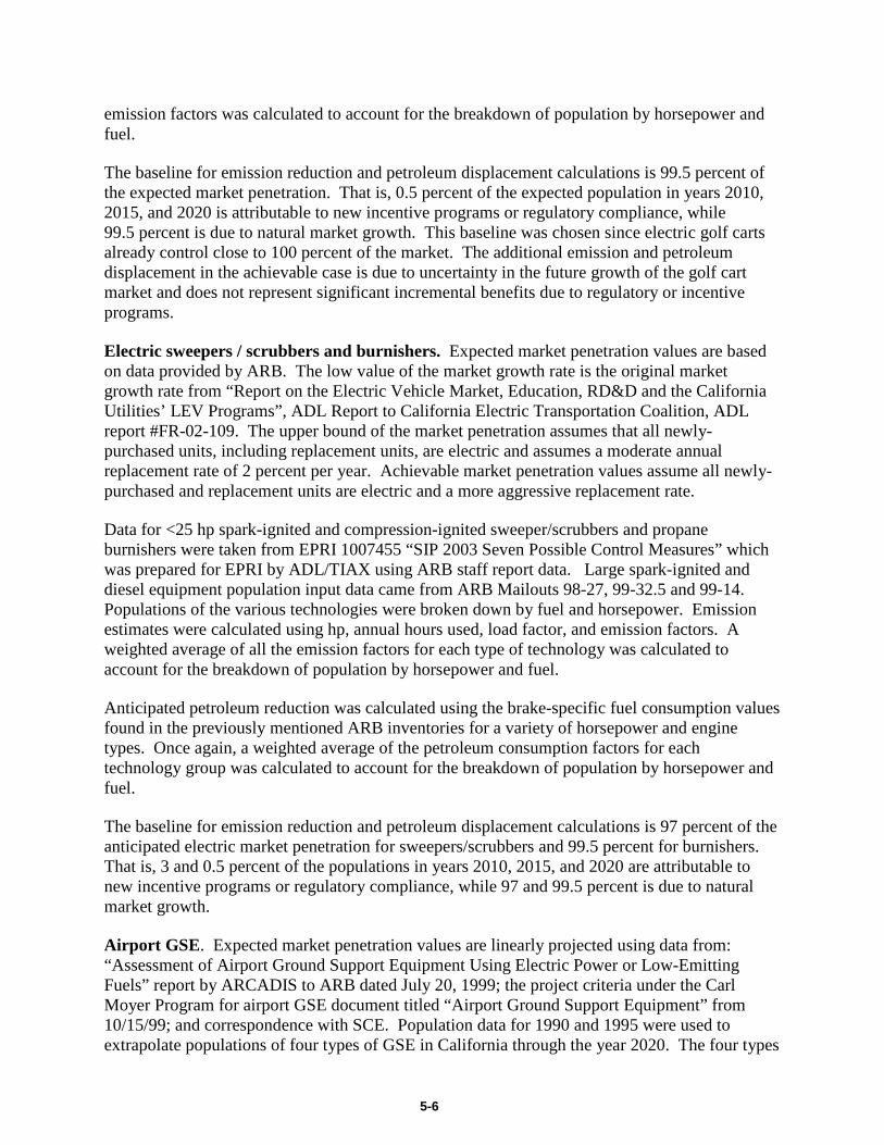
Electric golf carts. Electric golf cart market share in California increased from about 50 percent in 1997 to near 100 percent today due to ARB regulations. Since the market share of electric golf carts is assumed to be close to 100 percent, the market penetration of this technology through the year 2020 is a question of the overall market growth of golf carts. Expected and achievable market penetration values were calculated from the EPRI “Non-Road Electric Vehicle Market Segment Analysis Report” (EPRI TR-107290, November 1996) and data on the National Golf Federation website (www.ngf.org). Over the 1990s, the number of golf carts per course in California is shown to increase. The lower bound of the expected market penetration assumes that the 2002 value of carts per course remains constant through the year 2020, while the number of golf courses increases at a constant annual growth rate of 1.5 percent relative to 2002. The upper bound assumes that the number of carts per course increases at a moderate growth rate. The moderate growth rate is assumed to be half the annual growth rate seen between the years 1990-1995. The number of golf courses in California is also assumed to increase at the 1.5 percent growth rate mentioned above. The achievable population assumes that the number of carts per course increases at the rate seen between the years 1990-1995. The number of golf courses in California is also assumed to increase at the 1.5 percent growth rate mentioned above.

Emissions data for spark-ignited golf carts was taken from EPRI 1007455 “SIP 2003 Seven Possible Control Measures” (data for Burden & Personnel carriers/Turf trucks), which was prepared for EPRI by ADL/ TIAX using ARB staff report data. Turf truck emission factors were used in place of golf cart emission factors because these two technologies are similar. The population of golf carts was broken down by fuel and horsepower. Based on a brief survey of the current golf cart market, it was assumed that no diesel-powered or 50+ hp golf carts are commercially available. A breakdown of golf cart population by horsepower and engine type was assumed based on turf truck values; 90 percent of gasoline golf carts were assumed to be 4-stroke engines and the remainder 2-stroke. Emission estimates were calculated using hp, annual hours used, load factor, and NOx + ROG emission factors. A weighted average of all the

5-6

emission factors was calculated to account for the breakdown of population by horsepower and fuel.

The baseline for emission reduction and petroleum displacement calculations is 99.5 percent of the expected market penetration. That is, 0.5 percent of the expected population in years 2010, 2015, and 2020 is attributable to new incentive programs or regulatory compliance, while 99.5 percent is due to natural market growth. This baseline was chosen since electric golf carts already control close to 100 percent of the market. The additional emission and petroleum displacement in the achievable case is due to uncertainty in the future growth of the golf cart market and does not represent significant incremental benefits due to regulatory or incentive programs.

Electric sweepers / scrubbers and burnishers. Expected market penetration values are based on data provided by ARB. The low value of the market growth rate is the original market growth rate from “Report on the Electric Vehicle Market, Education, RD&D and the California Utilities’ LEV Programs”, ADL Report to California Electric Transportation Coalition, ADL report #FR-02-109. The upper bound of the market penetration assumes that all newly-purchased units, including replacement units, are electric and assumes a moderate annual replacement rate of 2 percent per year. Achievable market penetration values assume all newly-purchased and replacement units are electric and a more aggressive replacement rate.

Data for <25 hp spark-ignited and compression-ignited sweeper/scrubbers and propane burnishers were taken from EPRI 1007455 “SIP 2003 Seven Possible Control Measures” which was prepared for EPRI by ADL/TIAX using ARB staff report data. Large spark-ignited and diesel equipment population input data came from ARB Mailouts 98-27, 99-32.5 and 99-14. Populations of the various technologies were broken down by fuel and horsepower. Emission estimates were calculated using hp, annual hours used, load factor, and emission factors. A weighted average of all the emission factors for each type of technology was calculated to account for the breakdown of population by horsepower and fuel.

Anticipated petroleum reduction was calculated using the brake-specific fuel consumption values found in the previously mentioned ARB inventories for a variety of horsepower and engine types. Once again, a weighted average of the petroleum consumption factors for each technology group was calculated to account for the breakdown of population by horsepower and fuel.

The baseline for emission reduction and petroleum displacement calculations is 97 percent of the anticipated electric market penetration for sweepers/scrubbers and 99.5 percent for burnishers. That is, 3 and 0.5 percent of the populations in years 2010, 2015, and 2020 are attributable to new incentive programs or regulatory compliance, while 97 and 99.5 percent is due to natural market growth.

Airport GSE . Expected market penetration values are linearly projected using data from: “Assessment of Airport Ground Support Equipment Using Electric Power or Low-Emitting Fuels” report by ARCADIS to ARB dated July 20, 1999; the project criteria under the Carl Moyer Program for airport GSE document titled “Airport Ground Support Equipment” from 10/15/99; and correspondence with SCE. Population data for 1990 and 1995 were used to extrapolate populations of four types of GSE in California through the year 2020. The four types

5-7

are: baggage tugs, belt loaders, aircraft tug/pushback tractors, and air conditioning units. The lower bound of market penetration for these types of equipment assumes that all additions to the existing fleet are electric. The upper bound assumes that the half of the existing population plus all additions are electric, assuming the same overall annual growth rate found during 1990-1995.

Large spark-ignited and diesel equipment population input data came from ARB Mailouts 98-27, 99-32.5 and 99-14. Populations of the various technologies were broken down by fuel and horsepower. Emission estimates were calculated using hp, annual hours used, load factor, and emission factors. A weighted average of all the emission factors for each type of technology was calculated to account for the breakdown of population by horsepower and fuel.

The baseline for emission reduction and petroleum displacement calculations is 95 percent of the anticipated electric market penetration. That is, 5 percent of the population in years 2010, 2015, and 2020 is attributable to new incentive programs or regulatory compliance, while 95 percent is due to natural market growth.

Utility customers/airport GSE users report annual usage that ranges from 42 to 133 percent of ARB hours. ARB hours used in calculations above. Relative to the forklift category, GSE is a small contributor to the large-off-road equipment results: would affect the expected electricity consumption by at most 1 percent and the emissions by less than 10 percent.

Electric forklifts: Class 1 and 2. Expected population linearly projected from 2001 and 2006 population for class 1 and 2 electric and class 4 and 5 ICE forklifts provided in EPRI report TR-1007518 (Addendum to TR-109189, Electric Lift Trucks); achievable assumed extra 22,000 to 32,000 forklifts. Power and electricity rates were taken from data provided by CalETC member utilities based on testing and industry data. The NOx emission factors were taken from currently proposed LSI rule by ARB staff. ROG emissions, annual hours, and fuel consumption rates determined from ARB OFFROAD inventory emissions data. It was assumed that 1 to 8 percent of forklift growth displaced ICE forklifts under expected scenario. ARB brake-specific fuel consumption rate is 2 gallons/hour, when adjusting using the ARB load factor. Utility customers report rates of 1 to 2 gallons/hr in practice. If most forklifts actually consume 1 gallon per hour, the emissions and petroleum benefits would be half of the values shown. If the currently proposed LSI emission standards do not become law, the emissions displacement benefits would be 3-1/3 times greater than stated above. Scrap and buy programs targeting uncontrolled (i.e., pre-Model Year 2001) forklifts that are still in operation provide substantially more criteria pollutant emission benefits on a per unit basis (between 6 to 20 times the benefits per unit compared to replacing a controlled forklift). ARB staff reports for the current LSI rulemaking assume that such forklift will become increasingly scarce in the next decade due to natural turnover, and thus may not be available in sufficient quantities beyond 2010 to provide significant benefits under a scrap and buy program.

Electric forklifts. Class 3. Linearly projected from 2001 and 2006 population for class 3 electric forklifts provided in EPRI report TR-1007518 (Addendum to TR-109189, Electric Lift Trucks); class 3 is assumed to be all electric, achievable assumes additional 3 percent of projected population growth for class 3 to account for mode shifting (i.e., switching to narrow-aisle operations). Power and electricity rates were taken from data provided by CalETC member utilities. Emissions and fuel use based on same ARB data as discussed above.

5-8

Tow tractors / industrial tugs. Linear population projection and market fraction based on EPRI 1007455 “SIP 2003 Seven Possible Control Measures” which was prepared for EPRI by ADL / TIAX using ARB staff report data and assumes 60 percent market penetration, with 3.3 percent annual population growth; achievable assumed to be 95 percent total population; non-airport equipment only. One percent of the expected population was assumed to be incremental due to additional incentives and regulations. Emission factors assumed same as forklifts (see forklift methodology for discussion of the effect of pending LSI standards), annual hours taken from ARB data. Fuel consumption rate assumed to be same as for forklifts. Utility estimates for annual hours are as low as 340 compared to ARB’s 1800 hours/yr.

Electric personnel and burden carriers. Linearly projected 2010, 2015, 2020 population based on data from EPRI 1007455 “SIP 2003 Seven Possible Control Measures” which was prepared for EPRI by ADL / TIAX using ARB staff report data. The expected scenario assumes 2 percent growth rate in burden/personnel carrier population, electric market share does not change, and 1 percent of expected population assumed incremental due to regulations and incentives. Achievable scenario assumes an additional 14k (additional 32-37 percent), per the 2004 CalETC presentation to the California Environmental Protection Agency. Power and electricity rates taken from data provided by CalETC member utilities, emissions and fuel consumption taken from TIAX internal estimates based on ARB emission factors (see forklift methodology for discussion of the effect of pending LSI standards).

Turf trucks. No electric fraction of market initially, assumed 0 percent in 2010 and growth rate of electric fraction 2 percent/yr thereafter (growth rate experienced by ICE per EPRI 1007455). Achievable started at 25 percent, with 5 percent electric fraction growth per year. Power and electricity rates taken from SCE staff estimates, emissions and fuel consumption taken from data for EPRI 1007455 “SIP 2003 Seven Possible Control Measures” which was prepared for EPRI by ADL / TIAX using ARB staff report data.. All turf trucks are assumed to be incremental due to regulations and/or incentives.

Full-size, city, and neighborhood BEVs. Expected market penetration values are based on discussions with CalETC and its member utilities. The current population of full-size and city EVs in California are estimated at 1,000 total units, while NEVs are estimated at 10,000 units. The anticipated growth is approximately one or two thousand NEVs per year. In 2010, there are not expected to be many more full size BEVs or CEVs than today. After 2010, the annual market growth is estimated at 5 percent annual growth. Achievable population assumes that auto manufacturers choose to meet the ZEV program’s gold category alternate compliance pathway with half FCVs and half BEVs. The 50 percent compliance coming from BEVs is divided evenly between full size BEVs and city cars. NEVs do not meet the ZEV program’s gold category alternative compliance pathway. It was assumed that a full-size EV drives 13,322 miles and displaces a SULEV with LEV II DR total emissions (Reference: ARB ZEV program biennial review, August 7, 2000 Table 9-3) and a fuel efficiency of 21.2 miles/gallon (ARB/CEC Petroleum Dependency report see footnote 5; 21.1 refers to California light-duty vehicle, on-road fuel economy for 2002). For a city BEV and NEV, annual mileage estimates are 4,000 and 1,258 miles, respectively. Fuel efficiency for these technologies is assumed to be 30 miles/gallon. Electricity rates are based on industry estimates (.35 kWh/mi for full-size and .275 kWh/mi for city cars and NEVs). Using these values, an ICE counterpart full size BEV, city car, and NEV would consume 628.4, 133.3, and 41.9 gallons per year, respectively.

5-9

The baseline for emission reduction and petroleum displacement calculations is based on the following justification. Since the ZEV program is already in place, the current vehicles will not generate emission reduction benefits. Additionally, since the manufacturers will not make BEVs to meet the ZEV program under the expected case, any growth in the market can be assumed to displace conventional vehicle emissions. The market growth, however, would come from some form of incentives. Under the achievable scenario, everything over the existing populations of full-size, city car, and NEVs is displacing emissions because manufacturers do not have to make them, but chose to anyway.

Plug-in hybrid EVs. Population calculations are based on the assumption that the plug-in hybrid market will follow the same market trend as hybrid-electric vehicles (with a commercial market start date of 2010). It was assumed that a PHEV drives 13,322 miles based on polling data from the HEV Working Group report by EPRI in September 2001 and displaces a SULEV with LEV II DR total emissions (Reference: ARB ZEV program biennial review, August 7, 2000 Table 9-3) and a fuel efficiency of 21.2 miles/gallon. A PHEV20 operating 5,276 miles on electricity and 8,046 miles on gasoline per year is used to calculate the lower bound of connected load, electricity, emission, and petroleum reduction calculations. A PHEV60 operating 10,120 miles on electricity and 3,202 miles on gasoline is used to calculate the other upper bound values. Emissions factors for upstream emissions came from the petroleum dependency study (see footnote 5).

Hydrogen fuel cell vehicles. Vehicle implementation for FCVs assumed 100 percent of the ARB ZEV program’s “Gold Standard” category. Further assumptions were: hydrogen produced by steam reformation of natural gas; hydrogen vehicles driving 13,322 miles per year, displacing a SULEV with LEV II DR total emissions (Reference: ARB ZEV program biennial review, August 7, 2000); and a fuel efficiency of 42.4 miles per gasoline gallon equivalent. Achievable population assumes that all gold standard vehicles are FCVs and an additional 25 percent FCVs. Upstream emissions for natural gas are from the petroleum dependency study (footnote 5, Appendix A, Table 2-4). The electricity required to produce hydrogen is an industry estimate of 7.99 kWh / kg hydrogen for 2010 and 4.0 kWh / kg hydrogen for 2015 and later. Hydrogen ICE vehicles were not considered.

APPENDIX

A-1

Table A -1.A Expected Population Projections and Electric Fraction Expected Electric Population

(1000s, Unless Noted) Electric Fraction of Total

Population Technologies 2002a 2010 2015 2020 2010 2015 2020

Truck stop electrification (TSE) .20 (spaces)

8 - 10 (spaces)

10 - 14 (spaces)

14 - 19 (spaces)

27% 36% 49%

Ports: cold ironing (alternative marine power) .002 (ships)

0.020 (ships)

0.060 (ships)

0.129 (ships)

Port cargo handling equipment NA 0.191 (cranes)

0.193 (cranes)

0.195 (cranes)

100% 100% 100%

Electrified transportation refrigeration units (e-TRUs) 3.6b 9.1 11.7 16.9 up to 17% up to 21% up to 27%

Airport GSE 0.22 1.1 - 2.3 1.6 - 2.8 2.1 - 3.3 >30% >41% >46%

Electric forklifts: Class 1 and 2 35 33-55 40-65 47-75 45% 48% 51%

Tow tractors / industrial tugs 6.5 9 10 12 60% 60% 60%

Electric golf carts 57 - 67 74 - 82 80 - 92 85 - 103 >95% >95% >95%

Electric lawn and garden equipment (from new SORE list)

7.2 millionc 8.0 million 8.5 million 9.0 million 38% 38% 38%

Electric sweepers / scrubbers 123 27 - 28 28 - 30 28 - 31 up to 83% up to 85% up to 87%

Burnishers see above 101 - 102 104 - 104 106 - 107 98% 99% 99%

Electric forklifts: Class 3 34 53 60 67 100% 100% 100%

Electric personnel and burden carriers 30 37 40 44 65% 65% 65%

Turf trucks see above 0 3 7 <0.1% 10% 20%

Full-size, city and neighborhood BEVs 3.3 – 5.7 17 - 23 22 - 33 28 - 44 <0.1% <0.1% <0.1%

Plug-in hybrid EVs 0 10 138 543 0.1% 0.7% 2.1%

Hydrogen fuel cell vehicles NA 2 44 166 <0.1% 0.1% 0.6%

TOTAL 293 - 305 381 - 422 593 - 650 1171 - 1231 — — — a Values from original ADL LEV EV report or other source as noted; NA = not applicable or unavailable b Value from ARB TRU staff report dated October 2003

c Value from ARB off-road modeling technical memo, “Change in Population and Activity Factors for Lawn & Garden Equipment,” revised June 2003

A-2

Table A-1.B Achievable Population Projections

Achievable Population (1000s, Unless Noted) Technologies

2010 2015 2020

Truck stop electrification (TSE) 16 - 20

(spaces) 22 - 28

(spaces) 30 - 40

(spaces) Ports: cold ironing (alternative marine power) 0.123 (ships) 0.562 (ships) 1.201 (ships)

Port cargo handling equipment 0.191 (cranes) 0.193

(cranes) 0.195

(cranes)

Electrified transportation refrigeration units (e-TRUs)

13.5 25.5 34.9

Airport GSE 3.5 4 4.5

Electric forklifts: Class 1 and 2 55-87 66-97 77-107

Tow tractors / industrial tugs 14 16 19

Electric golf carts 89 103 117

Electric lawn and garden equipment (from new SORE list) 9.3 Million 11 Million 14.1 Million

Electric sweepers / scrubbers 29 32 35

Burnishers 103 106 109

Electric forklifts: Class 3 55 62 69

Electric personnel and burden carriers 51 54 57

Turf trucks 9.0 18.0 27.0

Full-size, city and neighborhood BEVs 36.4 209 455

Plug-in hybrid EVs 10 480 2112

Hydrogen fuel cell vehicles 2 56 208

TOTAL 487 - 523 1253 - 1290 3355 – 3446 a Values from original ADL LEV EV report or other source as noted; NA = not applicable or unavailable b Value from ARB TRU staff report dated October 2003 c Value from ARB off-road modeling technical memo, “Change in Population and Activity Factors for

Lawn & Garden Equipment,” revised June 2003

A-3

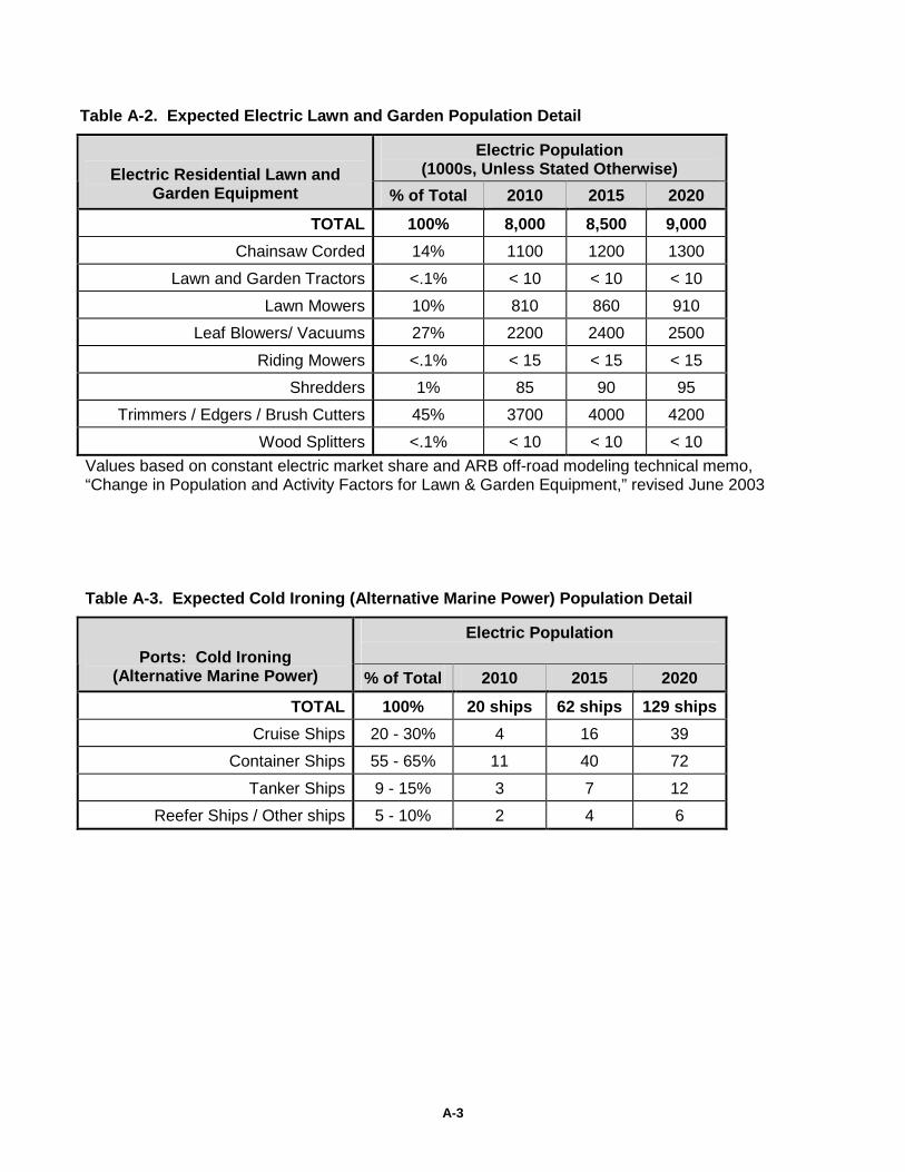
Table A-2. Expected Electric Lawn and Garden Population Detail

Electric Population (1000s, Unless Stated Otherwise) Electric Residential Lawn and

Garden Equipment % of Total 2010 2015 2020

TOTAL 100% 8,000 8,500 9,000

Chainsaw Corded 14% 1100 1200 1300

Lawn and Garden Tractors <.1% < 10 < 10 < 10

Lawn Mowers 10% 810 860 910

Leaf Blowers/ Vacuums 27% 2200 2400 2500

Riding Mowers <.1% < 15 < 15 < 15

Shredders 1% 85 90 95

Trimmers / Edgers / Brush Cutters 45% 3700 4000 4200

Wood Splitters <.1% < 10 < 10 < 10

Values based on constant electric market share and ARB off-road modeling technical memo, “Change in Population and Activity Factors for Lawn & Garden Equipment,” revised June 2003

Table A-3. Expected Cold Ironing (Alternative Marine Power) Population Detail

Electric Population Ports: Cold Ironing

(Alternative Marine Power) % of Total 2010 2015 2020

TOTAL 100% 20 ships 62 ships 129 ships

Cruise Ships 20 - 30% 4 16 39

Container Ships 55 - 65% 11 40 72

Tanker Ships 9 - 15% 3 7 12

Reefer Ships / Other ships 5 - 10% 2 4 6

A-4

Table A-4. Technology Drivers/Barriers and Governmental Mandates

Equipment Category Key Technology Drivers/Barriers Changes in Legislative/Governmental

Mandates and Incentives

Truck stop electrification (TSE)

Barriers: infrastructure costs. Drivers: new technology from IdleAire solves “chicken and egg” problem of infrastructure, as any truck can use this type of TSE. Several other firms are in the market in recent years, including shorepower types of TSE and battery APUs.

Federal: Bush Admin Energy Plan and 2003 Budget, and Climate Change Plan and USEPA “Climate Leaders” program. CA: 2005: Adopt anti-idling regulation for sleeper cabs to go into effect in 2009. (Truckers get option of diesel APU or electrification.) 2004: ARB voted to adopt an HD idling emissions reductions requirement. WDDERC has selected TSE as one of its main focuses in 2005. TSE is eligible for expanded Moyer incentive program, caps don’t apply to TSE—this may cover some or all of the infrastructure costs. CMAQ does fund TSE (how most have been funded to date). EPA announced fine $ would help to fund I-5 corridor TSE. Energy bill pending wtih $90 million included for TSE.

Ports: cold ironing (alternative marine power)

Barriers: More than half the vessels visiting the ports only visit once, is very expensive, and could be a major randomly occurring power draw, requiring upstream changes to infrastructure/power management. Drivers: Fifty-year-old technology used by Navy ships. Ten or so new demonstrations in world in last 10 years, including Port of LA.

Federal: Bush Admin Energy Plan and 2003 Budget, and Climate Change Plan and USEPA “Climate Leaders” program. CA: ARB New Shore Power Rule to reduce emissions from diesel auxiliary engines. ARB's Clean Air Plan for next 20 years. Is eligible for Moyer $, no net increase, the first commercial berth location and ship installation successful, and the planning of future sites in process.

Port cargo handling equipment

CA: EPA’s no net increase rule for port emissions.

Electrified transportation refrigeration units (e-TRUs)

Barriers: Require electrical infrastructure and different equipment; there is a potential for a mandate in this area. Drivers: e-TRUs are a clean and cost-effective alternative to diesel

CA: 2004: ARB adoption of ATCM for TRUs.

Electric lawn and garden equipment

Drivers: Electric options are less expensive; improvements in batteries and cost have made the techs more available. Trade-in programs have helped get techs into the market.

CA: Covered in the CA SIP.

Full-size, city and neighborhood EVs

Drivers: GHG emission standards, ZEV rule, fleet use. Barriers: Battery limitations and price.

Federal: Tax credits, Bush Admin Energy Plan and 2003 Budget, and Climate Change Plan and USEPA “Climate Leaders” program. CA: ARB's Clean Air Plan for next 20 years.

Plug-in hybrid EVs Drivers: Existing hybrid technology. Barriers: Technology not commercialized yet.

ARB ZEV program, GHG emissions standards (AB 32), Low-Carbon Fuel Standard (LCFS)

Electric golf carts Drivers: lower maintenance cost, lower first cost, quiet, smooth. Barriers: lower battery life over hilly terrain

100% new purchases in federal ozone non-attainment areas must be electric; those in attainment areas must follow small off-road engine regulations. Currently close to 100% market share. Growth limited to growth in golf cart demand.

Electric sweepers / scrubbers

Barriers: Performance limited by large battery and low run time (solution = fast charge and battery change-out technology); closely linked to battery / fuel cell technology; Drivers: Low maintenance cost, operate over flat terrain.

Carl Moyer Program: possible source of funds.

Burnishers Same as above Same as above

Airport GSE

Drivers: High availability, variety of models, airport demo projects, fast charge technology, ETEC Energy Delivery System (EDS), sealed batteries, low maintenance cost, flat terrain

Carl Moyer Program - source of funds; 1997 Existing Fleet Emissions Rate Goal; 1997 Existing Fleet ZEV Goal; New GSE ZEV Goal; SCAQMD airports must meet 2010 targets for tugs, tractors and belt loaders of 30% ZEV for existing fleet and 45% ZEV for new fleet; Technology Demo Program

A-5

Table A-4. Technology Drivers/Barriers, and Governmental Mandates (continued)

Equipment Category Key Technology Drivers/Barriers Changes in Legislative/Governmental

Mandates and Incentives

Electric forklifts: Class 1 and 2

Barriers: Sometimes difficult to have centralized charging infrastructure at older sites, requiring additional stations (additional capital cost). Drivers: Lower life-cycle cost of operation, especially with rising fuel costs; trend toward narrow-aisle operations; use-appropriate equipment

ARB LSI / DRR rules may foster adoption of electrics; commitment to permanent Moyer funds.

Electric forklifts: Class 3

Drivers: This is a more appropriate size technology for many applications than using oversized Class 4 and 5. Barriers: Class 3 doesn’t have an ICE equivalent—would need to increase demand for this type of lift truck.

Tow tractors Barriers: Charging infrastructure/equipment capital needed. Drivers: Widespread use, lower life-cycle cost of operation.

ARB LSI / DRR rules may foster adoption of electrics; commitment to permanent Moyer funds.

Electric personnel / burden carriersc

See above. ARB LSI / DRR rules may foster adoption of electrics; could employ measure requiring electric use, like with golf carts.

Turf trucks See above. See above.


Barriers: Life-cycle cost/kg fuel produced much higher than conventional fuel. Drivers: Number of demonstration programs increasing

CA Governor’s Hydrogen Highway program exploring ways to develop hydrogen infrastructure in near term; AB32 GHG Emission Reductions; LCFS

A-5-1

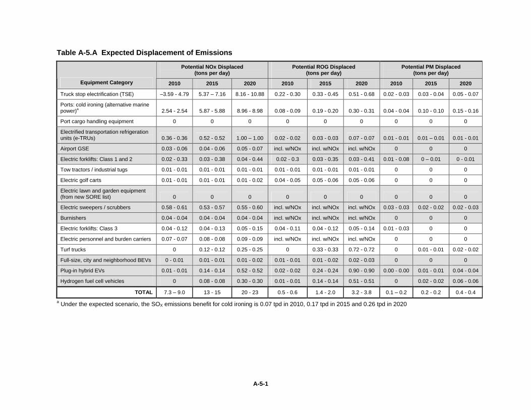
Table A-5.A Expected Displacement of Emissions

Potential NOx Displaced (tons per day)

Potential ROG Displaced (tons per day)

Potential PM Displaced (tons per day)

Equipment Category 2010 2015 2020 2010 2015 2020 2010 2015 2020

Truck stop electrification (TSE) –3.59 - 4.79 5.37 – 7.16 8.16 - 10.88 0.22 - 0.30 0.33 - 0.45 0.51 - 0.68 0.02 - 0.03 0.03 - 0.04 0.05 - 0.07

Ports: cold ironing (alternative marine power)a 2.54 - 2.54 5.87 - 5.88 8.96 - 8.98 0.08 - 0.09 0.19 - 0.20 0.30 - 0.31 0.04 - 0.04 0.10 - 0.10 0.15 - 0.16

Port cargo handling equipment 0 0 0 0 0 0 0 0 0

Electrified transportation refrigeration units (e-TRUs) 0.36 - 0.36 0.52 - 0.52 1.00 – 1.00 0.02 - 0.02 0.03 - 0.03 0.07 - 0.07 0.01 - 0.01 0.01 – 0.01 0.01 - 0.01

Airport GSE 0.03 - 0.06 0.04 - 0.06 0.05 - 0.07 incl. w/NOx incl. w/NOx incl. w/NOx 0 0 0

Electric forklifts: Class 1 and 2 0.02 - 0.33 0.03 - 0.38 0.04 - 0.44 0.02 - 0.3 0.03 - 0.35 0.03 - 0.41 0.01 - 0.08 0 – 0.01 0 - 0.01

Tow tractors / industrial tugs 0.01 - 0.01 0.01 - 0.01 0.01 - 0.01 0.01 - 0.01 0.01 - 0.01 0.01 - 0.01 0 0 0

Electric golf carts 0.01 - 0.01 0.01 - 0.01 0.01 - 0.02 0.04 - 0.05 0.05 - 0.06 0.05 - 0.06 0 0 0

Electric lawn and garden equipment (from new SORE list) 0 0 0 0 0 0 0 0 0

Electric sweepers / scrubbers 0.58 - 0.61 0.53 - 0.57 0.55 - 0.60 incl. w/NOx incl. w/NOx incl. w/NOx 0.03 - 0.03 0.02 - 0.02 0.02 - 0.03

Burnishers 0.04 - 0.04 0.04 - 0.04 0.04 - 0.04 incl. w/NOx incl. w/NOx incl. w/NOx 0 0 0

Electric forklifts: Class 3 0.04 - 0.12 0.04 - 0.13 0.05 - 0.15 0.04 - 0.11 0.04 - 0.12 0.05 - 0.14 0.01 - 0.03 0 0

Electric personnel and burden carriers 0.07 - 0.07 0.08 - 0.08 0.09 - 0.09 incl. w/NOx incl. w/NOx incl. w/NOx 0 0 0

Turf trucks 0 0.12 - 0.12 0.25 - 0.25 0 0.33 - 0.33 0.72 - 0.72 0 0.01 - 0.01 0.02 - 0.02

Full-size, city and neighborhood BEVs 0 - 0.01 0.01 - 0.01 0.01 - 0.02 0.01 - 0.01 0.01 - 0.02 0.02 - 0.03 0 0 0

Plug-in hybrid EVs 0.01 - 0.01 0.14 - 0.14 0.52 - 0.52 0.02 - 0.02 0.24 - 0.24 0.90 - 0.90 0.00 - 0.00 0.01 - 0.01 0.04 - 0.04

Hydrogen fuel cell vehicles 0 0.08 - 0.08 0.30 - 0.30 0.01 - 0.01 0.14 - 0.14 0.51 - 0.51 0 0.02 - 0.02 0.06 - 0.06

TOTAL 7.3 – 9.0 13 - 15 20 - 23 0.5 - 0.6 1.4 - 2.0 3.2 - 3.8 0.1 – 0.2 0.2 - 0.2 0.4 - 0.4

a Under the expected scenario, the SOX emissions benefit for cold ironing is 0.07 tpd in 2010, 0.17 tpd in 2015 and 0.26 tpd in 2020

A-5-2

Table A-5.B Expected Displacement of Greenhouse Gases and Petroleum

Potential Gasoline Displaced (million gge/year)*

Potential GHG displaced (million tons per year) Equipment Category

2010 2015 2020 2010 2015 2020

Truck stop electrification (TSE) 10 - 13 15 - 19 22 - 29 0.09 - 0.12 0.13 - 0.18 0.20 - 0.27

Ports: cold ironing (alternative marine power)a 6.4 - 6.7 14.1 – 17.7 21.5 – 28.0 0.04 - 0.04 0.08 - 0.13 0.12 - 0.20

Port cargo handling equipment 0 0 0 0 0 0

Electrified transportation refrigeration units (e-TRUs) 1.1 - 1.1 2.0 - 2.0 4.6 - 4.6 0.01 - 0.01 0.02 - 0.02 0.04 - 0.04

Airport GSE 0.24 - 0.49 0.35 - 0.61 0.46 - 0.72 0 - 0.01 0 - 0.01 0.01 - 0.01

Electric forklifts: Class 1 and 2 1.2 - 16.3 1.5 - 19.3 1.75 - 22.3 0.01 - 0.19 0.02 - 0.22 0.02 - 0.26

Tow tractors / industrial tugs 0.54 - 0.54 0.63 - 0.63 0.72 - 0.72 0.01 - 0.01 0.01 - 0.01 0.01 - 0.01

Electric golf carts 0.5 - 0.5 0.5 - 0.6 0.6 - 0.7 0.01 - 0.01 0.01 - 0.01 0.01 - 0.01

Electric lawn and garden equipment (from new SORE list) 0 0 0 0 0 0

Electric sweepers / scrubbers 2.9 - 3 3 - 3.2 3 - 3.3 0.04 - 0.04 0.04 - 0.04 0.04 - 0.04

Burnishers 0.7 - 0.7 0.7 - 0.7 0.7 - 0.7 0.01 - 0.01 0.01 - 0.01 0.01 - 0.01

Electric forklifts: Class 3 2.0 - 5.9 2.2 - 6.7 2.5 - 7.5 0.02 - 0.07 0.03 - 0.08 0.03 - 0.09

Electric personnel and burden carriers 0.5 - 0.5 0.58 - 0.58 0.64 - 0.64 0.01 - 0.01 0.01 - 0.01 0.01 - 0.01

Turf trucks 0 2.1 - 2.1 4.5 - 4.5 0 0.02 - 0.02 0.05 - 0.05

Full-size, city and neighborhood BEVs 0.8 - 1.6 1.5 - 3 2.3 - 4.4 0.01 - 0.02 0.02 - 0.03 0.03 - 0.05

Plug-in hybrid EVs 4.8 - 4.8 64 - 64 242 - 242 0.06 - 0.06 0.75 - 0.75 2.84 - 2.84

Hydrogen fuel cell vehicles 0.64 - 0.64 14 - 14 52 - 52 0.01 - 0.01 0.14 - 0.14 0.52 - 0.52

TOTAL 32 - 56 121 - 154 360 - 402 0.31 - 0.58 1.27 - 1.65 3.93 - 4.41

a Under the expected scenario, the SOX emissions benefit for cold ironing is 0.07 tpd in 2010, 0.17 tpd in 2015 and 0.26 tpd in 2020

A-5-3

Table A-5.C Expected Electricity Demand

Cumulative Connected Load a

(MW) Annual Electricity Use

(million kWh) Unmitigated Summer Peak Load

(MW)


Truck stop electrification (TSE) 11 - 42 15 - 56 20 - 76 57 - 76 85 - 113 129 - 172 4.5 - 26 6.1 - 34.9 8.3 - 47

Ports: cold ironing (alternative marine power) 63 - 63 221 - 221 479 - 479 81 - 81 297 - 297 630 - 630 54 - 54 185 - 185 398 - 398

Port cargo handling equipment 306 - 306 309 - 309 312 - 312 16 - 16 26 – 26 44 - 44 154 - 154 155 - 155 158 - 158

Electrified transportation refrigeration units (e-TRUs) 64 - 64 96 - 96 174 - 174 63 - 83 91 - 129 161 - 246 9.6 - 13 13 - 18 21 - 30

Airport GSE 9 - 24 14 - 30 18 - 35 10 - 22 15 - 28 19 - 33 3.2 - 13 4.7 - 16 6.3 - 19

Electric forklifts: Class 1 and 2 211 - 440 255 - 520 300 - 600 274 - 457 332 - 540 390 - 623 53 - 110 64 - 130 75 - 152

Tow tractors / industrial tugs 18 – 35 21 - 41 23 - 47 53 - 79 62 - 92 70 - 105 4.4 - 8.8 5.2 - 10 5.9 - 12

Electric golf carts 74 – 98 80 - 111 85 - 124 84 - 92 89 - 104 95 - 116 22 - 30 24 - 33 25 - 37

Electric lawn and garden equipment (from new SORE list) 0 0 0 113 - 113 120 - 120 128 - 128 0.9 - 1.9 1 - 2 1.1 - 2.1

Electric sweepers / scrubbers 40 – 64 41 - 67 42 - 71 9 - 30 10 - 31 10 - 33 3 - 9.4 3.1 - 9.9 3.2 - 10

Burnishers 150 – 230 154 - 236 158 - 243 57 - 79 58 - 81 60 - 83 15 - 46 15 - 47 16 - 49

Electric forklifts: Class 3 106 – 212 120 - 240 134 - 268 83 - 83 94 - 94 105 - 105 27 - 53 30 - 60 34 - 67

Electric personnel and burden carriers 37 – 51 40 - 56 44 - 62 75 - 75 82 - 82 90 - 90 7.3 - 10 8.1 - 11 8.8 - 12

Turf trucks 0 3 - 4 7 - 9 0 9 - 9 20 - 20 0 0.6 - 0.9 1.4 - 1.9

Full-size, city and neighborhood BEVs 28 – 38 36 - 54 44 - 70 8 - 11 11 - 15 13 - 19 7.6 - 18 10 - 26 12 - 33

Plug-in hybrid EVs 14 – 19 193 - 262 767 - 1041 20 - 30 273 - 525 1087 - 2035 1.4 - 3.8 19 – 52 77 - 208

Hydrogen fuel cell vehicles 1 – 1 6 - 6 24 - 24 5 - 5 55 - 55 207 - 207 0.5 - 0.5 6.2 - 6.2 23 - 23

TOTAL 1130 - 1688 1603 - 2312 2634 - 3642 1021 - 1356 1719 - 2354 3257 - 4737 365 - 556 550 - 798 872 - 1257

a The average rated load for a piece of equipment of that type multiplied by the electric population of that type given Table 3-1

A-5-4

Table A-6.A Achievable Displacement of Emissions

Potential NOx Displaced (tons per day)

Potential ROG Displaced

(tons per day)

Potential PM Displaced

(tons per day)


Truck stop electrification (TSE) 7.25 – 9.03 11.1 – 14.1 16.2 – 22.6 0.45 - 0.56 0.64 - 0.88 1.06 - 1.41 0.04 - 0.05 0.07 - 0.08 0.10 - 0.14

Ports: cold ironing (alternative marine power)a 5.12 - 5.12 29.75 - 29.77

43.17 - 43.20 0.17 - 0.18 0.99 - 1.03 1.56 - 1.63 0.09 - 0.09 0.50 - 0.50 0.79 - 0.80

Port cargo handling equipment 0 0 0 0 0 0 0 0 0

Electrified transportation refrigeration units (e-TRUs) 1.08 - 1.08 2.27 - 2.27 3.14 - 3.14 0.05 - 0.05 0.13 - 0.13 0.20 - 0.20 0.04 - 0.04 0.05 - 0.05 0.05 - 0.05

Airport GSE 0.78 - 0.78 0.58 - 0.58 0.59 - 0.59 incl. w/NOx incl. w/NOx incl. w/NOx 0.03 - 0.03 0.02 - 0.02 0.02 - 0.02

Electric forklifts: Class 1 and 2 1.65 - 2.69 1.95 - 2.75 2.25 - 2.80 1.51 - 2.47 1.79 - 2.52 2.06 - 2.57 0.04 - 0.06 0.04 - 0.06 0.05 - 0.06

Tow tractors / industrial tugs 0.39 - 0.39 0.45 - 0.45 0.52 - 0.52 0.36 - 0.36 0.42 - 0.42 0.48 - 0.48 0.01 - 0.01 0.01 - 0.01 0.01 - 0.01

Electric golf carts 0.24 - 0.24 0.36 - 0.36 0.46 - 0.46 0.88 - 0.88 1.32 - 1.32 1.72 - 1.72 0.03 - 0.03 0.04 - 0.04 0.06 - 0.06

Electric lawn and garden equipment (from new SORE list) 0.55 - 0.62 1.33 - 1.48 3.10 - 3.40 6.11 - 7.59 8.88 - 11.81

10.47 - 16.44 0.07 - 0.12 0.77 - 0.87 1.8 - 2.0

Electric sweepers / scrubbers 1.21 - 1.21 2.1 - 2.1 3.1 - 3.1 incl. w/NOx incl. w/NOx incl. w/NOx 0.06 - 0.06 0.09 - 0.09 0.13 - 0.13

Burnishers 0.17 - 0.17 0.17 - 0.17 0.16 - 0.16 incl. w/NOx incl. w/NOx incl. w/NOx 0.01 - 0.01 0.01 - 0.01 0.01 - 0.01

Electric forklifts: Class 3 0.19 - 0.27 0.19 - 0.28 0.20 - 0.30 0.17 - 0.24 0.18 - 0.26 0.18 - 0.27 0 - 0.01 0 - 0.01 0.01 - 0.01

Electric personnel and burden carriers 2.87 - 2.87 2.74 - 2.74 2.62 - 2.62 incl. w/NOx incl. w/NOx incl. w/NOx 0.12 - 0.12 0.11 - 0.11 0.11 - 0.11

Turf trucks 0.34 - 0.34 0.68 - 0.68 1.02 - 1.02 0.95 - 0.95 1.91 - 1.91 2.86 - 2.86 0.03 - 0.03 0.06 - 0.06 0.09 - 0.09

Full-size, city and neighborhood BEVs 0.02 - 0.02 0.19 - 0.19 0.43 - 0.43 0.03 - 0.03 0.31 - 0.31 0.73 - 0.73 0 0.03 - 0.03 0.07 - 0.07

Plug-in hybrid EVs 0.01 - 0.01 0.48 - 0.48 2.04 - 2.04 0.02 - 0.02 0.83 - 0.83 3.54 - 3.54 0.00 - 0.00 0.03 - 0.03 0.14 - 0.14

Hydrogen fuel cell vehicles 0 0.1 - 0.1 0.37 - 0.37 0.01 - 0.01 0.17 - 0.17 0.64 - 0.64 0 0.02 - 0.02 0.07 - 0.07

TOTAL 22 - 25 54 – 58 84 - 91 11 - 13 18 - 22 26 - 33 0.6 - 0.7 1.9 - 2.0 3.5 - 3.8

a Under the achievable scenario, the SOX emissions benefit for cold ironing is 0.10 tpd in 2010, 0.39 tpd in 2015 and 0.65 tpd in 2020

A-5-5

Table A-6.B Achievable Displacement of Greenhouse Gases and Petroleum

Potential Gasoline Displaced (million gge/year)*

Potential GHG Displaced (million tons/year)

Equipment Category 2010 2015 2020 2010 2015 2020

Truck stop electrification (TSE) 19.5 – 24.4 29.9 – 38.0 45.8 – 61.1 0.18 - 0.23 0.28 - 0.35 0.43 - 0.57

Ports: cold ironing (alternative marine power)a 12.2 – 18.4 71.2 – 92.8

112.8 - 149.5 0.07 - 0.14 0.39 - 0.67 0.61 - 1.10

Port cargo handling equipment 0 0 0 0 0 0

Electrified transportation refrigeration units (e-TRUs) 3.4 - 3.4 9.2 - 9.2 13.9 - 13.9 0.03 – 0.03 0.09 - 0.09 0.13 - 0.13

Airport GSE 5.7 - 5.7 5.8 - 5.8 5.9 - 5.9 0.07 – 0.07 0.07 - 0.07 0.07 - 0.07

Electric forklifts: Class 1 and 2 83 - 135.2 98.1 - 138.2

113.2 - 141.2 0.96 – 1.56 1.13 - 1.59 1.31 - 1.63

Tow tractors / industrial tugs 19.6 - 19.6 22.9 - 22.9 26.1 - 26.1 0.22 – 0.23 0.26 - 0.27 0.3 - 0.31

Electric golf carts 9.6 - 9.6 14.4 - 14.4 18.9 - 18.9 0.12 – 0.12 0.17 - 0.17 0.23 - 0.23

Electric lawn and garden equipment (from new SORE list) 5 - 16 10 - 29 18 - 50 0.06 – 0.19 0.11 - 0.33 0.2 - 0.58

Electric sweepers / scrubbers 6 - 6 11.6 - 11.6 17.2 - 17.2 0.07 – 0.07 0.14 - 0.14 0.21 - 0.21

Burnishers 3 - 3 2.8 - 2.8 2.6 - 2.6 0.04 – 0.04 0.03 - 0.03 0.03 - 0.03

Electric forklifts: Class 3 9 - 13 10 - 14 10 - 15 0.11 – 0.16 0.12 - 0.17 0.12 - 0.18

Electric personnel and burden carriers 21.3 - 21.3 20.4 - 20.4 19.5 - 19.5 0.25 - 0.25 0.24 - 0.24 0.23 - 0.23

Turf trucks 6 - 6 12 - 12 18 - 18 0.06 - 0.06 0.13 - 0.13 0.19 - 0.19

Full-size, city and neighborhood BEVs 5.5 - 5.5 55 - 55 131 - 131 0.06 - 0.06 0.53 - 0.53 1.24 - 1.24

Plug-in hybrid EVs 4.8 – 4.8 221.2 - 221.2

926.2 - 926.2 0.06 - 0.06 2.6 - 2.6 10.8 - 10.8

Hydrogen fuel cell vehicles 0.75 - 0.75 17.4 - 17.4 65.2 - 65.2 0.01 - 0.01 0.17 - 0.17 0.65 - 0.65

TOTAL 214 - 293 612 - 705 1544 - 1661 2.4 - 3.6 6.5 - 7.6 16.8 - 18.2

a Under the achievable scenario, the SOX emissions benefit for cold ironing is 0.10 tpd in 2010, 0.39 tpd in 2015 and 0.65 tpd in 2020.

A-5-6

Table A-6.C Achievable Electricity Demand

Cumulative Connected Load a

(MW) Annual Electricity Use

(million kWh) Unmitigated Summer Peak Load

(MW)


Truck stop electrification (TSE) 22 – 78 30 - 110 41 - 157 114 - 143 175 - 222 268 - 357 9 - 47 12 - 66 16 - 94

Ports: cold ironing (alternative marine power)a 225 – 225 1222 - 1222 2530 - 2530 65 - 65 160 - 160 287 - 287 200 - 200 1052 - 1052 2187 - 2187

Port cargo handling equipment 306 – 306 309 - 309 312 - 312 16 - 16 26 - 26 44 - 44 154 - 154 155 - 155 157 - 157

Electrified transportation refrigeration units (e-TRUs) 130 – 130 304 - 304 444 - 444 120 - 183 311 - 440 462 - 651 16 - 23 33 - 49 48 - 70

Airport GSE 29 – 37 34 - 42 38 - 48 29 - 33 34 - 38 38 - 44 10 - 20 11 - 23 13 - 26

Electric forklifts: Class 1 and 2 351 – 696 421 - 776 491 - 856 457 - 722 548 - 805 639 - 888 88 - 174 105 - 194 123 - 124

Tow tractors / industrial tugs 28 – 56 32 - 65 37 - 74 84 - 125 97 - 146 111 - 167 7 - 14 8 - 16 9.5 - 19

Electric golf carts 89 – 107 103 - 124 117 - 140 100 - 100 116 - 116 132 - 132 27 - 32 31 - 37 35 - 42

Electric lawn and garden equipment (from new SORE list) 0 0 0 185 - 185 197 - 197 209 - 209 1.1 - 2.1 1.3 - 2.5 1.6 - 3.3

Electric sweepers / scrubbers 43 – 66 47 - 72 52 - 79 10 - 30 11 - 34 12 - 37 3.3 - 10 3.6 - 11 3.9 - 12

Burnishers 153 – 234 157 - 240 161 - 246 58 - 80 60 - 82 61 - 85 15 - 47 16 - 48 16 - 49

Electric forklifts: Class 3 110 – 220 124 - 248 138 - 276 86 - 86 97 - 97 108 - 108 28 - 55 31 - 62 35 - 69

Electric personnel and burden carriers 51 – 71 54 - 76 57 - 80 104 - 104 110 - 110 116 - 116 10 - 14 11 - 15 11 - 16

Turf trucks 9 – 13 18 - 25 27 - 38 27 - 27 54 - 54 81 - 81 1.8 - 2.5 3.6 - 5 5.4 - 7.6

Full-size, city and neighborhood BEVs 76 – 93 579 - 791 1325 - 1825 41 - 41 416 - 416 986 - 986 17 - 40 100 - 318 216 - 721

Plug-in hybrid EVs 14 – 19 672 - 912 2957 - 4013 595 - 1142 2976 - 6660 4960 - 9514 1.4 – 3.8 67 - 182 296 - 803

Hydrogen fuel cell vehicles 1 – 1 8 - 8 30 - 30 6 - 6 69 - 69 259 - 259 0.7 - 0.7 7.7 - 7.7 29 - 29

TOTAL 1638 - 2353 4115 - 5324 8759 - 11151 2097 - 3088 5456 - 9672 8773 - 13920 588 - 838 1650 - 2244 3202 - 4518

a The average rated load for a piece of equipment of that type multiplied by the electric population of that type given Table 3-1

electric transportation technologies in · pdf fileelectric transportation and goods movement...

Documents