electrical energy systems - erdinç kuruoğlu · electrical energy systems. series ed. ... reserves...

El-Hawary, M.E. “The Energy Control Center”Electrical Energy Systems.Series Ed. Leo GrigsbyBoca Raton: CRC Press LLC, 2000

299

© 2000 CRC Press LLC

Chapter 8

THE ENERGY CONTROL CENTER

8.1 INTRODUCTION

The following criteria govern the operation of an electric powersystem:

• Safety• Quality• Reliability• Economy

The first criterion is the most important consideration and aims toensure the safety of personnel, environment, and property in every aspect ofsystem operations. Quality is defined in terms of variables, such as frequencyand voltage, that must conform to certain standards to accommodate therequirements for proper operation of all loads connected to the system.Reliability of supply does not have to mean a constant supply of power, but itmeans that any break in the supply of power is one that is agreed to and toleratedby both supplier and consumer of electric power. Making the generation costand losses at a minimum motivates the economy criterion while mitigating theadverse impact of power system operation on the environment.

Within an operating power system, the following tasks are performed inorder to meet the preceding criteria:

• Maintain the balance between load and generation.• Maintain the reactive power balance in order to control the voltage

profile.• Maintain an optimum generation schedule to control the cost and

environmental impact of the power generation.• Ensure the security of the network against credible contingencies.

This requires protecting the network against reasonable failure ofequipment or outages.

The fact that the state of the power network is ever changing becauseloads and networks configuration change, makes operating the system difficult.Moreover, the response of many power network apparatus is not instantaneous.For example, the startup of a thermal generating unit takes a few hours. Thisessentially makes it not possible to implement normal feed-forward control.Decisions will have to be made on the basis of predicted future states of thesystem.

Several trends have increased the need for computer-based operatorsupport in interconnected power systems. Economy energy transactions, reliance

300


on external sources of capacity, and competition for transmission resources haveall resulted in higher loading of the transmission system. Transmission linesbring large quantities of bulk power. But increasingly, these same circuits arebeing used for other purposes as well: to permit sharing surplus generatingcapacity between adjacent utility systems, to ship large blocks of power fromlow-energy-cost areas to high-energy cost areas, and to provide emergencyreserves in the event of weather-related outages. Although such transfers havehelped to keep electricity rates lower, they have also added greatly to the burdenon transmission facilities and increased the reliance on control.

Heavier loading of tie-lines which were originally built to improvereliability, and were not intended for normal use at heavy loading levels, hasincreased interdependence among neighboring utilities. With greater emphasison economy, there has been an increased use of large economic generating units.This has also affected reliability.

As a result of these trends, systems are now operated much closer tosecurity limits (thermal, voltage and stability). On some systems, transmissionlinks are being operated at or near limits 24 hours a day. The implications are:

• The trends have adversely affected system dynamic performance.A power network stressed by heavy loading has a substantiallydifferent response to disturbances from that of a non-stressedsystem.

• The potential size and effect of contingencies has increaseddramatically. When a power system is operated closer to the limit,a relatively small disturbance may cause a system upset. Thesituation is further complicated by the fact that the largest sizecontingency is increasing. Thus, to support operating functionsmany more scenarios must be anticipated and analyzed. Inaddition, bigger areas of the interconnected system may be affectedby a disturbance.

• Where adequate bulk power system facilities are not available,special controls are employed to maintain system integrity.Overall, systems are more complex to analyze to ensure reliabilityand security.

• Some scenarios encountered cannot be anticipated ahead of time.Since they cannot be analyzed off-line, operating guidelines forthese conditions may not be available, and the system operatormay have to “improvise” to deal with them (and often does). As aresult, there is an ever increasing need for mechanisms to supportdispatchers in the decision making process. Indeed, there is a riskof human operators being unable to manage certain functionsunless their awareness and understanding of the network state isenhanced.

To automate the operation of an electric power system electric utilitiesrely on a highly sophisticated integrated system for monitoring and control.

301


Such a system has a multi-tier structure with many levels of elements. Thebottom tier (level 0) is the high-reliability switchgear, which includes facilitiesfor remote monitoring and control. This level also includes automaticequipment such as protective relays and automatic transformer tap-changers.Tier 1 consists of telecontrol cabinets mounted locally to the switchgear, andprovides facilities for actuator control, interlocking, and voltage and currentmeasurement. At tier 2, is the data concentrators/master remote terminal unitwhich typically includes a man/machine interface giving the operator access todata produced by the lower tier equipment. The top tier (level 3) is thesupervisory control and data acquisition (SCADA) system. The SCADA systemaccepts telemetered values and displays them in a meaningful way to operators,usually via a one-line mimic diagram. The other main component of a SCADAsystem is an alarm management subsystem that automatically monitors all theinputs and informs the operators of abnormal conditions.

Two control centers are normally implemented in an electric utility,one for the operation of the generation-transmission system, and the other forthe operation of the distribution system. We refer to the former as the energymanagement system (EMS), while the latter is referred to as the distributionmanagement system (DMS). The two systems are intended to help thedispatchers in better monitoring and control of the power system. The simplestof such systems perform data acquisition and supervisory control, but many alsohave sophisticated power application functions available to assist the operator.Since the early sixties, electric utilities have been monitoring and controllingtheir power networks via SCADA, EMS, and DMS. These systems provide the“smarts” needed for optimization, security, and accounting, and indeed arereally formidable entities. Today’s EMS software captures and archives livedata and records information especially during emergencies and systemdisturbances.

An energy control center represents a large investment by the powersystem ownership. Major benefits flowing from the introduction of this systeminclude more reliable system operation and improved efficiency of usage ofgeneration resources. In addition, power system operators are offered more in-depth information quickly. It has been suggested that at Houston Lighting &Power Co., system dispatchers’ use of network application functions (such asPower Flow, Optimal Power Flow, and Security Analysis) has resulted inconsiderable economic and intangible benefits. A specific example of $ 70,000in savings achieved through avoiding field crew overtime cost, and by leavingequipment out of service overnight is reported for 1993. This is part of a total of$ 340,000 savings in addition to increased system safety, security and reliabilityhas been achieved through regular and extensive use of just some networkanalysis functions.

8.2 OVERVIEW OF EMS FUNCTIONS

System dispatchers at the EMS are required to make short-term (next

302


day) and long-term (prolonged) decisions on operational and outage schedulingon a daily basis. Moreover, they have to be always alert and prepared to dealwith contingencies that may arise occasionally. Many software and hardwarefunctions are required as operational support tools for the operator. Broadlyspeaking, we can classify these functions in the following manner:

• Base functions• Generation functions• Network functions

Each of these functions is discussed briefly in this section.

Base Functions

The required base functions of the EMS include:

• The ability to acquire real time data from monitoring equipmentthroughout the power system.

• Process the raw data and distribute the processed data within thecentral control system.

Data acquisition (DA) acquires data from remote terminal units (RTUs)installed throughout the system using special hardware connected to the realtime data servers installed at the control center. Alarms that occur at thesubstations are processed and distributed by the DA function. In addition,protection and operation of main circuit breakers, some line isolators,transformer tap changers and other miscellaneous substation devices areprovided with a sequence of events time resolution.

Data Acquisition

The data acquisition function collects, manages, and processesinformation from the RTUs by periodically scanning the RTUs and presentingthe raw analog data and digital status points to a data processing function. Thisfunction converts analog values into engineering units and checks the digitalstatus points for change since the previous scan so that an alarm can be raised ifstatus has changed. Computations can be carried out and operating limits can beapplied against any analog value such that an alarm message is created if a limitis violated.

Supervisory Control

Supervisory control allows the operator to remotely control all circuitbreakers on the system together with some line isolators. Control of devices canbe performed as single actions or a line circuit can be switched in or out ofservice.

303


Alarm Processor

The alarm processor software is responsible to notify the operator ofchanges in the power system or the computer control system. Manyclassification and detection techniques are used to direct the alarms to theappropriate operator with the appropriate priorities assigned to each alarm.

Logical Alarming

This provides the facility to predetermine a typical set of alarmoperations, which would result from a single cause. For example, a faultedtransmission line would be automatically taken out of service by the operation ofprotective and tripping relays in the substation at each end of the line and theautomatic opening of circuit breakers. The coverage would identify theprotection relays involved, the trip relays involved and the circuit breakers thatopen. If these were defined to the system in advance, the alarm processor wouldcombine these logically to issue a priority 1 alarm that the particular powercircuit had tripped correctly on protection. The individual alarms would then begiven a lower priority for display. If no logical combination is viable for theparticular circumstance, then all the alarms are individually presented to thedispatcher with high priority. It is also possible to use the output of a logicalalarm as the indicator for a sequence-switching procedure. Thus, the EMSwould read the particular protection relays which had operated and restore a lineto service following a transient fault.

Sequence of Events Function

The sequence of events function is extremely useful for post-mortemanalysis of protection and circuit breaker operations. Every protection relay, triprelay, and circuit breaker is designated as a sequence of events digital point.This data is collected, and time stamped accurately so that a specified resolutionbetween points is possible within any substation and across the system.Sequence of events data is buffered on each RTU until collected by dataacquisition automatically or on demand.

Historical Database

Another function includes the ability to take any data obtained by thesystem and store in a historical database. It then can be viewed by a tabular orgraphical trend display. The data is immediately stored within the on-linesystem and transferred to a standard relational data base system periodically.Generally, this function allows all features of such database to be used toperform queries and provide reports.

Automatic Data Collection

This function is specified to define the process taken when there is amajor system disturbance. Any value or status monitored by the system can be

304


defined as a trigger. This will then cause a disturbance archive to be created,which will contain a pre-disturbance and a post-disturbance snapshots to beproduced.

Load Shedding Function

This facility makes it possible to identify that particular load block andinstruct the system to automatically open the correct circuit breakers involved.It is also possible to predetermine a list of load blocks available for loadshedding. The amount of load involved within each block is monitored so thatwhen a particular amount of load is required to shed in a system emergency, theoperator can enter this value and instruct the system to shed the appropriateblocks.

Safety Management

Safety management provided by an EMS is specific to each utility. Asystem may be specified to provide the equivalent of diagram labeling and paperbased system on the operator’s screen. The software allows the engineer, havingopened isolators and closed ground switches on the transmission system, todesignate this as safety secured. In addition, free-placed ground symbols can beapplied to the screen-based diagram. A database is linked to the diagram systemand records the request for plant outage and safety document details. Thecomputer system automatically marks each isolator and ground switch beingpresently quoted on a safety document and records all safety documents usingeach isolator or ground switch. These details are immediately available at anyoperating position when the substation diagram is displayed.

Generation Functions

The main functions that are related to operational scheduling of thegenerating subsystem involve the following:

• Load forecasting• Unit commitment• Economic dispatch and automatic generation control (AGC)• Interchange transaction scheduling

Each of these functions is discussed briefly here.

Load Forecasting

The total load demand, which is met by centrally dispatched generatingunits, can be decomposed into base load and controlled load. In some systems,there is significant demand from storage heaters supplied under an economytariff. The times at which these supplies are made available can be altered usingradio tele-switching. This offers the utility the ability to shape the total demandcurve by altering times of supply to these customers. This is done with the

305


objective of making the overall generation cost as economic andenvironmentally compatible as possible. The other part of the demand consistsof the uncontrolled use of electricity, which is referred to as the natural demand.It is necessary to be able to predict both of these separately. The base demand ispredicted using historic load and weather data and a weather forecast.

Unit Commitment

The unit commitment function determines schedules for generationoperation, load management blocks and interchange transactions that candispatched. It is an optimization problem, whose goal is to determine unitstartup and shutdown and when on-line, what is the most economic output foreach unit during each time step. The function also determines transfer levels oninterconnections and the schedule of load management blocks. The softwaretakes into account startup and shutdown costs, minimum up and down times andconstraints imposed by spinning reserve requirements.

The unit commitment software produces schedules in advance for thenext time period (up to as many as seven days, at 15-minute intervals). Thealgorithm takes the predicted base demand from the load forecasting functionand the predicted sizes of the load management blocks. It then places the loadmanagement blocks onto the base demand curve, essentially to smooth itoptimally. The operator is able to use the software to evaluate proposedinterchange transactions by comparing operating costs with and without theproposed energy exchange. The software also enables the operator to computedifferent plant schedules where there are options on plant availability

Economic Dispatch and AGC

The economic dispatch (ED) function allocates generation outputs ofthe committed generating units to minimize fuel cost, while meeting systemconstraints such as spinning reserve. The ED functions to computerecommended economic base points for all manually controlled units as well aseconomic base points for units which may be controlled directly by the EMS.

The Automatic Generation Control (AGC) part of the softwareperforms dispatching functions including the regulation of power output ofgenerators and monitoring generation costs and system reserves. It is capable ofissuing control commands to change generation set points in response tochanges in system frequency brought about by load fluctuations.

Interchange Transaction Scheduling Function

This function allows the operator to define power transfer schedules ontie-lines with neighboring utilities. In many instances, the function evaluates theeconomics and loading implications of such transfers.

306


Current Operating Plan (COP)

As part of the generation and fuel dispatch functions on the EMS at atypical utility is a set of information called the Current Operating Plan (COP)which contains the latest load forecast, unit commitment schedule, and hourlyaverage generation for all generating units with their forecast operating status.The COP is typically updated every 4 to 8 hours, or as needed following majorchanges in load forecast and/or generating unit availability.

Network Analysis Functions

Network applications can be subdivided into real-time applications andstudy functions. The real time functions are controlled by real time sequencecontrol that allows for a particular function or functions to be executedperiodically or by a defined event manually. The network study functionsessentially duplicate the real time function and are used to study any number of“what if” situations. The functions that can be executed are:

• Topology Processing (Model Update) Function.• State Estimation Function.• Network Parameter Adaptation Function• Dispatcher Power Flow (DPF)• Network Sensitivity Function.• Security Analysis Function.• Security Dispatch Function• Voltage Control Function• Optimal Power Flow Function

Topology Processing (Model Update) Function

The topology processing (model-updating) module is responsible forestablishing the current configuration of the network, by processing thetelemetered switch (breakers and isolators) status to determine existingconnections and thus establish a node-branch representation of the system.

State Estimation Function

The state estimator function takes all the power system measurementstelemetered via SCADA, and provides an accurate power flow solution for thenetwork. It then determines whether bad or missing measurements usingredundant measurements are present in its calculation. The output from the stateestimator is given on the one-line diagram and is used as input to otherapplications such as Optimal Power Flow.

Network Parameter Adaptation Function

This module is employed to generate forecasts of busbar voltages and

307


loads. The forecasts are updated periodically in real time. This allows the stateestimator to schedule voltages and loads at busbars where no measurements areavailable.

Dispatcher Power Flow (DPF)

A DPF is employed to examine the steady state conditions of anelectrical power system network. The solution provides information on networkbus voltages (kV), and transmission line and transformer flows (MVA). Thecontrol center dispatchers use this information to detect system violations(over/under-voltages, branch overloads) following load, generation, andtopology changes in the system.

Network Sensitivity Function

In this function, the output of the state estimator is used to determinethe sensitivity of network losses to changes in generation patterns or tie-lineexchanges. The sensitivity parameters are then converted to penalty factors foreconomic dispatch purposes.

Security Analysis Function

The SA is one of the main applications of the real time networkanalysis set. It is designed to assist system dispatchers in determining the powersystem security under specified single contingency and multiple contingencycriteria. It helps the operator study system behavior under contingencyconditions. The security analysis function performs a power flow solution foreach contingency and advises of possible overloads or voltage limit violations.The function automatically reviews a list of potential problems, rank them as totheir effect and advise on possible reallocation of generation. The objective ofOSA is to operate the network closer to its full capability and allow the properassessment of risks during maintenance or unexpected outages.

Security Dispatch Function

The security dispatch function gives the operator a tool with thecapability of reducing or eliminating overloads by rearranging the generationpattern. The tool operates in real-time on the network in its current state, ratherthan for each contingency. The function uses optimal power flow and constrainseconomic dispatch to offer a viable security dispatch of the generating resourcesof the system.

Voltage Control Function

The voltage control (VC) study is used to eliminate or reduce voltageviolations, MVA overloads and/or minimize transmission line losses usingtransformer set point controls, generator MVAR, capacitor/reactor switching,load shedding, and transaction MW.

308


Optimal Power Flow Function

The purpose of the Optimal Power Flow (OPF) is to calculaterecommended set points for power system controls that are a trade-off betweensecurity and economy. The primary task is to find a set of system states within aregion defined by the operating constraints such as voltage limits and branchflow limits. The secondary task is to optimize a cost function within this region.Typically, this cost function is defined to include economic dispatch of activepower while recognizing network-operating constraints. An important limitationof OPF is that it does not optimize switching configurations.

Optimal power flow can be integrated with other EMS functions ineither a preventive or corrective mode. In the preventive mode, the OPF is usedto provide suggested improvements for selected contingency cases. These casesmay be the worst cases found by contingency analysis or planned outages.

In the corrective mode, an OPF is run after significant changes in thetopology of the system. This is the situation when the state estimation outputindicates serious violations requiring the OPF to reschedule the active andreactive controls.

It is important to recognize that optimization is only possible if thenetwork is controllable, i.e., the control center must have control of equipmentsuch as generating units or tap-changer set points. This may present a challengeto an EMS that does not have direct control of all generators. To obtain the fullbenefit of optimization of the reactive power flows and the voltage profile, it isimportant to be able to control all voltage regulating devices as well asgenerators.

The EMS network analysis functions (e.g., Dispatcher Power Flow andSecurity Analysis) are the typical tools for making many decisions such asoutage scheduling. These tools can precisely predict whether the outage of aspecific apparatus (i.e., transformer, generator, or transmission line) would causeany system violations in terms of abnormal voltages or branch overloads.

In a typical utility system, outage requests are screened based on thesystem violation indications from DPF and SA studies. The final approval forcrew scheduling is granted after the results from DPF and SA are reviewed.

Operator Training Simulator

An energy management system includes a training simulator thatallows system operators to be trained under normal operating conditions andsimulated power system emergencies. System restoration may also beexercised. It is important to realize that major power system events arerelatively rare, and usually involve only one shift team out of six, realexperience with emergencies builds rather slowly. An operator-trainingsimulator helps maintain a high level of operational preparedness among thesystem operators.

309


The interface to the operator appears identical to the normal controlinterface. The simulator relies on two models: one of the power system and theother represents the control center. Other software is identical to that used inreal time. A scenario builder is available such that various contingencies can besimulated through a training session. The instructor controls the scenarios andplays the role of an operator within the system.

8.3 POWER FLOW CONTROL

The power system operator has the following means to control systempower flows:

1. Prime mover and excitation control of generators.2. Switching of shunt capacitor banks, shunt reactors, and static var

systems.3. Control of tap-changing and regulating transformers.4. FACTS based technology.

A simple model of a generator operating under balanced steady-stateconditions is given by the Thévenin equivalent of a round rotor synchronousmachine connected to an infinite bus as discussed in Chapter 3. V is thegenerator terminal voltage, E is the excitation voltage, δ is the power angle, andX is the positive-sequence synchronous reactance. We have shown that:

δsinX

EVP =

[ ]VEX

VQ −= δcos

The active power equation shows that the active power P increaseswhen the power angle δ increases. From an operational point of view, when theoperator increases the output of the prime mover to the generator while holdingthe excitation voltage constant, the rotor speed increases. As the rotor speedincreases, the power angle δ also increases, causing an increase in generatoractive power output P. There is also a decrease in reactive power output Q,given by the reactive power equation. However, when δ is less than 15°, theincrease in P is much larger than the decrease in Q. From the power-flow pointof view, an increase in prime-mover power corresponds to an increase in P atthe constant-voltage bus to which the generator is connected. A power-flowprogram will compute the increase in δ along with the small change in Q.

The reactive power equation demonstrates that reactive power output Qincreases when the excitation voltage E increases. From the operational point ofview, when the generator exciter output increases while holding the prime-mover power constant, the rotor current increases. As the rotor currentincreases, the excitation voltage E also increases, causing an increase in

310


generator reactive power output Q. There is also a small decrease in δ requiredto hold P constant in the active power equation. From the power-flow point ofview, an increase in generator excitation corresponds to an increase in voltagemagnitude at the infinite bus (constant voltage) to which the generator isconnected. The power-flow program will compute the increase in reactivepower Q supplied by the generator along with the small change in δ.

The effect of adding a shunt capacitor bank to a power-system bus canbe explained by considering the Thévenin equivalent of the system at that bus.This is simply a voltage source VTh in series with the impedance Zsys. The busvoltage V before connecting the capacitor is equal to VTh. After the bank isconnected, the capacitor current IC leads the bus voltage V by 90°. Constructinga phasor diagram of the network with the capacitor connected to the bus revealsthat V is larger than VTh. From the power-flow standpoint, the addition of ashunt capacitor bank to a load bus corresponds to the addition of a reactivegenerating source (negative reactive load), since a capacitor produces positivereactive power (absorbs negative reactive power). The power-flow programcomputes the increase in bus voltage magnitude along with a small change in δ.Similarly, the addition of a shunt reactor corresponds to the addition of apositive reactive load, wherein the power flow program computes the decreasein voltage magnitude.

Tap-changing and voltage-magnitude-regulating transformers are usedto control bus voltages as well as reactive power flows on lines to which theyare connected. In a similar manner, phase-angle-regulating transformers areused to control bus angles as well as real power flows on lines to which they areconnected. Both tap changing and regulating transformers are modeled by atransformer with an off-nominal turns ratio. From the power flow point of view,a change in tap setting or voltage regulation corresponds to a change in tap ratio.The power-flow program computes the changes in Ybu bus voltage magnitudesand angles, and branch flows.

FACTS is an acronym for flexible AC transmission systems. They usepower electronic controlled devices to control power flows in a transmissionnetwork so as to increase power transfer capability and enhance controllability.The concept of flexibility of electric power transmission involves the ability toaccommodate changes in the electric transmission system or operatingconditions while maintaining sufficient steady state and transient margins.

A FACTS controller is a power electronic-based system and other staticequipment that provide control of one or more ac transmission systemparameters. FACTS controllers can be classified according to the mode of theirconnection to the transmission system as:

1. Series-Connected Controllers.2. Shunt-Connected Controllers.3. Combined Shunt and Series-Connected Controllers.

311


The family of series-connected controllers includes the followingdevices:

1. The Static Synchronous Series Compensator (S3C) is a static,synchronous generator operated without an external electric energysource as a series compensator whose output voltage is inquadrature with, and controllable independently of, the line currentfor the purpose of increasing or decreasing the overall reactivevoltage drop across the line and thereby controlling the transmittedelectric power. The S3C may include transiently rated energystorage or energy absorbing devices to enhance the dynamicbehavior of the power system by additional temporary real powercompensation, to increase or decrease momentarily, the overall real(resistive) voltage drop across the line.

2. Thyristor Controlled Series Compensation is offered by animpedance compensator, which is applied in series on an actransmission system to provide smooth control of series reactance.

3. Thyristor Switched Series Compensation is offered by animpedance compensator, which is applied in series on an actransmission system to provide step-wise control of seriesreactance.

4. The Thyristor Controlled Series Capacitor (TCSC) is a capacitivereactance compensator which consists of a series capacitor bankshunted by thyristor controlled reactor in order to provide asmoothly variable series capacitive reactance.

5. The Thyristor Switched Series Capacitor (TSSC) is a capacitivereactance compensator which consists of a series capacitor bankshunted by thyristor controlled reactor in order to provide astepwise control of series capacitive reactance.

6. The Thyristor Controlled Series Reactor (TCSR) is an inductivereactance compensator which consists of a series reactor shuntedby thyristor controlled reactor in order to provide a smoothlyvariable series inductive reactance.

7. The Thyristor Switched Series Reactor (TSSR) is an inductivereactance compensator which consists of a series reactor shuntedby thyristor controlled reactor in order to provide a stepwisecontrol of series inductive reactance.

Shunt-connected Controllers include the following categories:

1. A Static Var Compensator (SVC) is a shunt connected static vargenerator or absorber whose output is adjusted to exchangecapacitive or inductive current so as to maintain or control specificparameters of the electric power system (typically bus voltage).SVCs have been in use since the early 1960s. The SVC applicationfor transmission voltage control began in the late 1970s.

2. A Static Synchronous Generator (SSG) is a static, self-commutatedswitching power converter supplied from an appropriate electric

312


energy source and operated to produce a set of adjustable multi-phase output voltages, which may be coupled to an ac powersystem for the purpose of exchanging independently controllablereal and reactive power.

3. A Static Synchronous Compensator (SSC or STATCOM) is astatic synchronous generator operated as a shunt connected staticvar compensator whose capacitive or inductive output current canbe controlled independent of the ac system voltage.

4. The Thyristor Controlled Braking Resistor (TCBR) is a shunt-connected, thyristor-switched resistor, which is controlled to aidstabilization of a power system or to minimize power accelerationof a generating unit during a disturbance.

5. The Thyristor Controlled Reactor (TCR) is a shunt-connected,thyristor-switched inductor whose effective reactance is varied in acontinuous manner by partial conduction control of the thyristorvalve.

6. The Thyristor Switched Capacitor (TSC) is a shunt-connected,thyristor-switched capacitor whose effective reactance is varied ina stepwise manner by full or zero-conduction operation of thethyristor valve.

The term Combined Shunt and Series-Connected Controllers is used todescribe controllers such as:

1. The Unified Power Flow Controller (UPFC) can be used to controlactive and reactive line flows. It is a combination of a staticsynchronous compensator (STATCOM) and a static synchronousseries compensator (S3C) which are coupled via a common dc link.This allows bi-directional flow of real power between the seriesoutput terminals of the S3C and the shunt output terminals of theSTATCOM, and are controlled to provide concurrent real andreactive series line compensation without an external electricenergy source. The UPFC, by means of angularly unconstrainedseries voltage injection, is capable of controlling, concurrently orselectively, the transmission line voltage, impedance, and angle or,alternatively, the real and reactive power flow in the line. TheUPFC may also provide independently controllable shunt reactivecompensation.

2. The Thyristor Controlled Phase Shifting Transformer (TCPST) is aphase shifting transformer, adjusted by thyristor switches toprovide a rapidly variable phase angle.

3. The Interphase Power Controller (IPC) is a series-connectedcontroller of active and reactive power consisting of, in each phase,of inductive and capacitive branches subjected to separately phase-shifted voltages. The active and reactive power can be setindependently by adjusting the phase shifts and/or the branchimpedances, using mechanical or electronic switches. In theparticular case where the inductive and capacitive impedances

313


form a conjugate pair, each terminal of the IPC is a passive currentsource dependent on the voltage at the other terminal.

The significant impact that FACTS devices will make on transmissionsystems arises because of their ability to effect high-speed control. Presentcontrol actions in a power system, such as changing transformer taps, switchingcurrent or governing turbine steam pressure, are achieved through the use ofmechanical devices, which impose a limit on the speed at which control actioncan be made. FACTS devices are capable of control actions at far higherspeeds. The three parameters that control transmission line power flow are lineimpedance and the magnitude and phase of line end voltages. Conventionalcontrol of these parameters is not fast enough for dealing with dynamic systemconditions. FACTS technology will enhance the control capability of thesystem.

A potential motivation for the accelerated use of FACTS is thederegulation/competitive environment in contemporary utility business. FACTShave the potential ability to control the path of the flow of electric power, andthe ability to effectively join electric power networks that are not wellinterconnected. This suggests that FACTS will find new applications as electricutilities merge and as the sale of bulk power between distant exchange partnersbecomes more wide spread.

8.4 POWER FLOW

Earlier chapters of this book treated modeling major components of anelectric power system for analysis and design purposes. In this section weconsider the system as a whole. An ubiquitous EMS application software is thepower flow program, which solves for network state given specified conditionsthroughout the system. While there are many possible ways for formulating thepower flow equations, the most popular formulation of the network equations isbased on the nodal admittance form. The nature of the system specificationsdictates that the network equations are nonlinear and hence no direct solution ispossible. Instead, iterative techniques have to be employed to obtain a solution.As will become evident, good initial estimates of the solution are important, anda technique for getting started is discussed. There are many excellent numericalsolution methods for solving the power flow problem. We choose here tointroduce the Newton-Raphson method.

Network Nodal Admittance Formulation

Consider a power system network shown in Figure 8.1 with generatingcapabilities as well as loads indicated. Buses 1, 2, and 3 are buses havinggeneration capabilities as well as loads. Bus 3 is a load bus with no realgeneration. Bus 4 is a net generation bus.

Using the π equivalent representation for each of the lines, we obtain

314


Figure 8.1 Single-Line Diagram to Illustrate Nodal Matrix Formulation.

the network shown in Figure 8.2. Let us examine this network in which weexclude the generator and load branches. We can write the current equations as

( ) ( )( ) ( )( ) ( ) ( )( )

34

233413

2312

1312

344044

2343133033

32122022

31211011

L

LLL

LL

LL

YVVYVI

YVVYVVYVVYVI

YVVYVVYVI

YVVYVVYVI

−+=

−+−+−+=

−+−+=

−+−+=

We introduce the following admittances:

34

23

13

12

34

342313

2312

1312

4334

3223

3113

2112

4044

3033

2022

1011

L

L

L

L

L

LLL

LL

LL

YYY

YYY

YYY

YYY

YYY

YYYYY

YYYY

YYYY

−==

−==

−==

−==

+=

+++=

++=

++=

315


Thus the current equations reduce to

444343214

4343332231133

43232221212

43132121111

00

0

0

VYVYVVI

VYVYVYVYI

VVYVYVYI

VVYVYVYI

+++=+++=+++=+++=

Note that Y14 = Y41 = 0, since buses 1 and 4 are not connected; also Y24 = Y42 = 0since buses 2 and 4 are not connected.

The preceding set of equations can be written in the nodal-matrixcurrent equation form:

busbusbus VYI = (8.1)

where the current vector is defined as

=

4

3

2

1

bus

I

I

I

I

I

The voltage vector is defined as

Figure 8.2 Equivalent Circuit for System of Figure 8.1.

316


=

4

3

2

1

bus

V

V

V

V

V

The admittance matrix is defined as

=

44342414

34332313

24232212

14131211

bus

YYYY

YYYY

YYYY

YYYY

Y

We note that the bus admittance matrix Ybus is symmetric.

The General Form of the Load-Flow Equations

The result obtained for the 4 bus network can be generalized to the caseof n buses. Here, each of vectors Ibus and Vbus are n × 1 vectors. The busadmittance matrix becomes and n × n matrix with elements

ijLjiij YYY −== (8.2)

∑=

=n

jLii ij

YY0

(8.3)

The summation is over the set of all buses connected to bus i including theground (node 0).

We recall that bus powers Si rather than the bus currents Ii are, inpractice, specified. We thus use

i

ii

V

SI =*

As a result, we have

( )∑=

=− n

jjij

i

ii VYV

jQP

1*

( )ni ,,1!= (8.4)

These are the static power flow equations. Each equation is complex, andtherefore we have 2n real equations.

317


The nodal admittance matrix current equation can be written in thepower form:

( ) ( )∑=

=−n

jjijiii VYVjQP

1

*(8.5)

The bus voltages on the right-hand side can be substituted for usingeither the rectangular form:

1jfeV ii +=

or the polar form:

ii

jii

V

ieVV

θ

θ

∠=

=

Rectangular Form

If we choose the rectangular form, then we have by substitution,

( ) ( )

++

−= ∑∑

==

n

jiijjiji

n

jiijjijii eBfGffBeGeP

11

(8.6)

( ) ( )

+−

−= ∑∑

==

n

jiijjiji

n

jiijjijii eBfGefBeGfQ

11

(8.7)

where the admittance is expressed in the rectangular form:

ijijij jBGY += (8.8)

Polar Form

On the other hand, if we choose the polar form, then we have

( )ijjij

n

jijii VYVP ψθθ −−= ∑

=

cos1

(8.9)

( )ijjij

n

jijii VYVQ ψθθ −−= ∑

=

sin1

(8.10)

318


where the admittance is expressed in the polar form:

ijijij YY ψ∠= (8.11)

Hybrid Form

An alternative form of the power flow equations is the hybrid form,which is essentially the polar form with the admittances expressed in rectangularform. Expanding the trigonometric functions, we have

( ) ( )[ ]ijjiijjij

n

jijii VYVP ψθθψθθ sinsincoscos

1

−+−= ∑=

(8.12)

( ) ( )[ ]ijjiijjij

n

jijii VYVQ ψθθψθθ sincoscossin

1

−−−= ∑=

(8.13)

Now we use

( )ijij

ijijijij

jBG

jYY

+=

+= ψψ sincos(8.14)

Separating the real and imaginary parts, we obtain

ijijij YG ψcos= (8.15)

ijijij YB ψsin= (8.16)

so that the power-flow equations reduce to

( ) ( )[ ]∑=

−+−=n

jjiijjiijjii BGVVP

1

sincos θθθθ (8.17)

( ) ( )[ ]∑=

−−−=n

jjiijjiijjii BGVVQ

1

cossin θθθθ (8.18)

The Power Flow Problem

The power-flow (or load-flow) problem is concerned with finding thestatic operating conditions of an electric power transmission system whilesatisfying constraints specified for power and/or voltage at the network buses.

319


Generally, buses are classified as follows:

1. A load bus (P-Q bus) is one at which Si = Pi +jQi is specified.2. A generator bus (P-V bus) is a bus with specified injected active

power and a fixed voltage magnitude.3. A system reference or slack (swing) bus is one at which both the

magnitude and phase angle of the voltage are specified. It iscustomary to choose one of the available P-V buses as slack and toregard its active power as the unknown.

As we have seen before, each bus is modeled by two equations. In all,we have 2n equations in 2n unknowns. These are V and θ at the load buses, Q

and θ at the generator buses, and the P and Q at the slack bus.

Let us emphasize here that due to the bus classifications, it is notnecessary for us to solve the 2n equations simultaneously. A reduction in therequired number of equations can be effected. What we do essentially is todesignate the unknown voltage magnitudes iV and angles θi at load buses and

θi at generator buses as primary unknowns. Once these values are obtained, thenwe can evaluate the secondary unknowns Pi and Qi at the slack bus and thereactive powers for the generator buses. This leads us to specifying thenecessary equations for a full solution:

1. At load buses, two equations for active and reactive powers areneeded.

2. At generator buses, with jV specified, only the active power

equation is needed.

Nonlinearity of the Power Flow Problem

Consider the power flow problem for a two-bus system with bus 1being the reference bus and bus 2 is the load bus. The unknown is 2V , and is

replaced by x.

2Vx =

222Y=α (8.19)

( ) 212

sp222

sp2222 YPGQB −−=β (8.20)

( )2sp2S=γ (8.21)

320


( ) ( ) ( )2sp2

2sp2

2sp2 QPS += (8.22)

We can demonstrate that the power flow equations reduce to the followingequation:

024 =++ γβα xx (8.23)

The solution to the fourth order equation is straightforward since wecan solve first for x2 as

ααγββ

2

422 −±−=x (8.24)

Since x2 cannot be imaginary, we have a first condition requiring that

042 ≥− αγβ

From the definitions of α, β, and γ, we can show that for a meaningful solutionto exist, we need to satisfy the condition:

( ) ( ) −++≥ sp

222sp

2222

122sp

222sp

2224

12 4 QGPBYQGPBY (8.25)

A second condition can be obtained if we observe that x cannot beimaginary, requiring that x2 be positive. Observing that α and γ are positive bytheir definition leads us to conclude that

βαγβ ≤−42

For x2 to be positive, we need

0≤β

or

( ) 022

12sp

222sp222 ≤−− YPGQB (8.26)

We can therefore conclude the following:

• There may be some specified operating conditions for which nosolution exists.

• More than one solution can exist. The choice can be narroweddown to a practical answer using further considerations.

321


Except for very simple networks, the load-flow problem results in a set ofsimultaneous algebraic equations that cannot be solved in closed form. It isnecessary to employ numerical iterative techniques that start by assuming a setof values of the unknowns and then repeatedly improve on their values in anorganized fashion until (hopefully) a solution satisfying the power flowequations is reached. The next section considers the question of gettingestimates (initial guess) for the unknowns.

Generating Initial Guess Solution

It is important to have a good approximation to the load-flow solution,which is then used as a starting estimate (or initial guess) in the iterativeprocedure. A fairly simple process can be used to evaluate a goodapproximation to the unknown voltages and phase angles. The process isimplemented in two stages: the first calculates the approximate angles, and thesecond calculates the approximate voltage magnitudes.

Busbar Voltage Angles Approximation

In this stage we make the following assumptions:

1. All angles are small, so that sin θ ≅ θ , cos θ ≅ 1.2. All voltage magnitudes are 1 p.u.

Applying these assumptions to the active power equations for thegenerator buses and load buses in hybrid form, we obtain

( ) ( )jiij

N

jiji BGP θθ −+=∑

=1

This is a system of N-1 simultaneous linear equations in θi, which is then solvedto obtain the busbar voltage angle approximations.

Busbar Voltage Magnitude Approximation

The calculation of voltage magnitudes employs the angles provided by theabove procedure. The calculation is needed only for load buses. We representeach unknown voltage magnitude as

ii VV ∆+=1

We also assume that

ii

VV

∆−≅∆+

11

1

322


By considering all load buses we obtain a linear system of simultaneousequations in the unknowns iV∆ . The results are much more reliable than the

commonly used flat-start process where all voltages are assumed to be 01∠ .

Newton-Raphson Method

The Newton-Raphson (NR) method is widely used for solvingnonlinear equations. It transforms the original nonlinear problem into asequence of linear problems whose solutions approach the solution of theoriginal problem. The method can be applied to one equation in one unknown orto a system of simultaneous equations with as many unknowns as equations.

One-Dimensional Case

Let F(x) be a nonlinear equation. Any value of x that satisfies F(x) = 0is a root of F(x). To find a particular root, an initial guess for x in the vicinity ofthe root is needed. Let this initial guess by x0. Thus

00)( FxF ∆=

where ∆F0 is the error since x0 is not a root. A tangent is drawn at the point onthe curve corresponding to x0, and is projected until it intercepts the x-axis todetermine a second estimate of the root. Again the derivative is evaluated, and atangent line is formed to proceed to the third estimate of x. The line generatedin this process is given by

))(()()( nnn xxxFxFxy −′+= (8.27)

which, when y(x) = 0, gives the recursion formula for iterative estimates of theroot:

( )( )n

nnn

xF

xFxx

′−=+1 (8.28)

N-Dimensional Case

The single dimensional concept of the Newton-Raphson method can beextend to N dimensions. All that is needed is an N-dimensional analog of thefirst derivative. The Jacobian matrix provides this. Each of the n rows of theJacobian matrix consists of the partial derivatives of one of the equations of thesystem with respect to each of the N variables.

An understanding of the general case can be gained from the specificexample N = 2. Assume that we are given the two nonlinear equations F1, F2.Thus,

0),( 211 =xxF 0),( 212 =xxF (8.29)

323


The Jacobian matrix for this 2 × 2 system is

∂∂

∂∂

∂∂

∂∂

2

2

1

2

2

1

1

1

x

F

x

F

x

F

x

F

(8.30)

If the Jacobian matrix is numerically evaluated at some point ( )(1

kx , )(2kx ), the

following linear relationship is established for small displacements ( 1x∆ , 2x∆ ):

∆

∆

=

∆

∆

∂∂

∂∂

∂∂

∂∂

+

+

)(2

)(1

)1(2

)1(1

2

)(2

1

)(2

2

)(1

1

)(1

k

k

k

k

kk

kk

F

F

x

x

x

F

x

F

x

F

x

F

(8.31)

A recursive algorithm can be developed for computing the vectordisplacements ( 1x∆ , 2x∆ ). Each displacement is a solution to the related linear

problem. With a good initial guess and other favorable conditions, the algorithm

will converge to a solution of the nonlinear problem. We let ( )0(1x , )0(

2x ) be the

initial guess. Then the errors are

[ ])0(2

)0(11

)0(1 , xxFF −=∆ , [ ])0(

2)0(

12)0(

2 , xxFF −=∆ (8.32)

The Jacobian matrix is then evaluated at the trial solution point [ )0(1x , )0(

2x ].

Each element of the Jacobian matrix is computed from an algebraic formula for

the appropriate partial derivative using )0(1x , )0(

2x . Thus,

∆

∆

=

∆

∆

∂∂

∂∂

∂∂

∂∂

)0(2

)0(1

)1(2

)1(1

2

)0(2

1

)0(2

2

)0(1

1

)0(1

F

F

x

x

x

F

x

F

x

F

x

F

(8.33)

This system of linear equations is then solved directly for the first correction.The correction is then added to the initial guess to complete the first iteration:

∆

∆+

=

)1(

2

)1(1

)0(2

)0(1

)1(2

)1(1

x

x

x

x

x

x(8.34)

324


Equations (8.33) and (8.34) are rewritten using matrix symbols and a generalsuperscript h for the iteration count;

[ ][ ] [ ]11 −− ∆=∆ hhh FxJ (8.35)

hhh xxx ∆+= −1 (8.36)

The algorithm is repeated until hF∆ satisfies some tolerance. In most solvableproblems it can be made practically zero.

The Newton-Raphson Method for Load-Flow Solution

There are different ways to apply the Newton-Raphson method tosolving the load-flow equations. We illustrate a popular version employing thepolar form. For each generator bus (except for the slack bus), we have theactive power equation and the corresponding unknown phase θi. We write thisequation in the form

0sch =−=∆ iii PPP

For each load bus we have the active and reactive equations and theunknowns iV and θi. We write the two equations in the form

0

0sch

sch

=−=∆

=−=∆

iii

iii

QQQ

PPP

In the above equations, the superscript “sch” denotes the schedules or specifiedbus active or reactive powers. We use the polar form to illustrate the process.

( )

( )ijji

n

jjijii

ijji

n

jjijii

VYVQ

VYVP

ψθθ

ψθθ

−−=

−−=

∑

∑

=

=

sin

cos

1

1

We show the application of the Newton-Raphson method to solve thepower flow problem. The incremental corrections to estimates of the unknownsare obtained as the solution to the linear system of equations. Thus, for theexample network we have:

325


( ) ( )

( ) ( )

( ) ( ) 333

33

3

32

2

3

333

33

3

32

2

3

233

23

3

22

2

2

QVV

QQQ

PVV

PPP

PVV

PPP

∆=∆∂∂+∆

∂∂+∆

∂∂

∆=∆∂∂+∆

∂∂+∆

∂∂

∆=∆∂∂+∆

∂∂+∆

∂∂

θθ

θθ

θθ

θθ

θθ

θθ

To simplify the calculation, the third term in each of the equations ismodified so that we solve for ( )33 VV∆ . We therefore have in matrix

notation:

∆

∆

∆

=

∆

∆

∆

∂∂

∂∂

∂∂

∂∂

∂∂

∂∂

∂∂

∂∂

∂∂

3

3

2

3

3

3

2

3

33

3

3

2

3

3

33

3

3

2

3

3

23

3

2

2

2

Q

P

P

V

VV

QV

QQ

V

PV

PP

V

PV

PP

θ

θ

θθ

θθ

θθ

Solving for ∆θ2, ∆θ3 and ( )33 VV∆ , we thus obtain the new estimates at the (h

+1)th iteration:

3)(

3)1(

3

3)(

3)1(

3

2)(

2)1(

2

VVVhh

hh

hh

∆+=

∆+=

∆+=

+

+

+

θθθ

θθθ

The application in the general case assumes that bus 1 is the slack bus,that buses 2, . . ., m are generator buses, and that buses m + 1, m + 2, . . ., n areload buses. We introduce the Van Ness variables:

j

iij

j

iij

QJ

PH

θ

θ

∂∂=

∂∂=

jj

iij

jj

iij

VV

QL

VV

PN

∂∂=

∂∂=

In condensed form, we have

326


∆

∆=

∆∆

Q

P

VV

LJ

NHθ

For the standpoint of computation, we use the rectangular form of thepower equations. We introduce

jijjijij

jijjijij

eBfGb

fBeGa

+=

−=

In terms of the aij and bij variables, we have

( ) ( )

( ) ( )∑∑

∑∑

==

==

−=

+=

n

jiji

n

jijii

n

jiji

n

jijii

beafQ

bfaeP

11

11

To summarize the expressions for the Van Ness variables are given by:

2

2

2

2

iiiiii

iiiiii

iiiiii

iiiiii

iijiijijij

iijiijijij

VGPJ

VGPN

VBQL

VBQH

fbeaJN

ebfaLH

−=

+=

−=

−−=

+=−=

−==

( )diagonals off ji ≠

A tremendous number of iterative techniques have been proposed tosolve the power flow problem. It is beyond the scope of this text to outlinemany of the proposed variations. The Newton-Raphson method has gained awide acceptability in industry circles, and as a result there are a number ofavailable computer packages that are based on this powerful method andsparsity-directed programming.

8.5 STABILITY CONSIDERATIONS

We are interested in the behavior of the system immediately followinga disturbance such as a short circuit on a transmission line, the opening of a line,or the switching on of a large block of loads. Studies of this nature are calledtransient stability analysis. The term stability is used in the sense of the ability

327


of the system machines to recover form small random perturbing forces and stillmaintain synchronism. In this section we give an introduction to transientstability in electric power system. We treat the case of a single machineoperating to supply an infinite bus. We do not deal with the analysis of the morecomplex problem of large electric power networks with the interconnectionstaken into consideration.

The Swing Equation

The dynamic equation relating the inertial torque to the net acceleratingtorque of the synchronous machine rotor is called the swing equation. Thissimply states

mN2

2

⋅=

aT

dt

dJ

θ(8.37)

The left-hand side is the inertial torque, which is the product of the inertia (inkg. m2) of all rotating masses attached to the rotor shaft and the angularacceleration. The accelerating torque Ta is in Newton meters and can beexpressed as

ema TTT −= (8.38)

In the above, Tm is the driving mechanical torque, and Te is the retarding or loadelectrical torque.

The angular position of the rotor θ may be expressed as:

δωαθ ++= tR (8.39)

The angle α is a constant that is needed if the angle δ is measured from an axisdifferent from the angular reference. The angle ωRt is the result of the rotorangular motion at rated speed. The angle δ is time varying and representsdeviations from the rated angular displacements. This is the basis for the newrelation

em TTdt

dJ −=

2

2δ(8.40)

It is more convenient to make the following substitution of the dot notation:

2

2

dt

d δδ =""

328


Therefore we have

em TTJ −=δ"" (8.41)

An alternative forms of Eq. (8.41) is the power form obtained bymultiplying both sides of Eq. (8.41) by ω and recalling that the product of thetorque T and angular velocity is the shaft power. This results in

em PPJ −=δω ""

The quantity Jω is called the inertia constant and is truly an angular momentumdenoted by M (Js/rad). As a result,

ωJM = (8.42)

Thus, the power form is

em PPM −=δ"" (8.43)

Concepts in Transient Stability

In order to gain an understanding of the concepts involved in transientstability prediction, we will concentrate on the simplified network consisting ofa series reactance X connecting the machine and the infinite bus. Under theseconditions the active power expression is given by:

δsinX

EVPe = (8.44)

This yields the power angle curve shown in Figure 8.3.

Figure 8.3 Power Angle Curve Corresponding to Eq. (8.44).

329


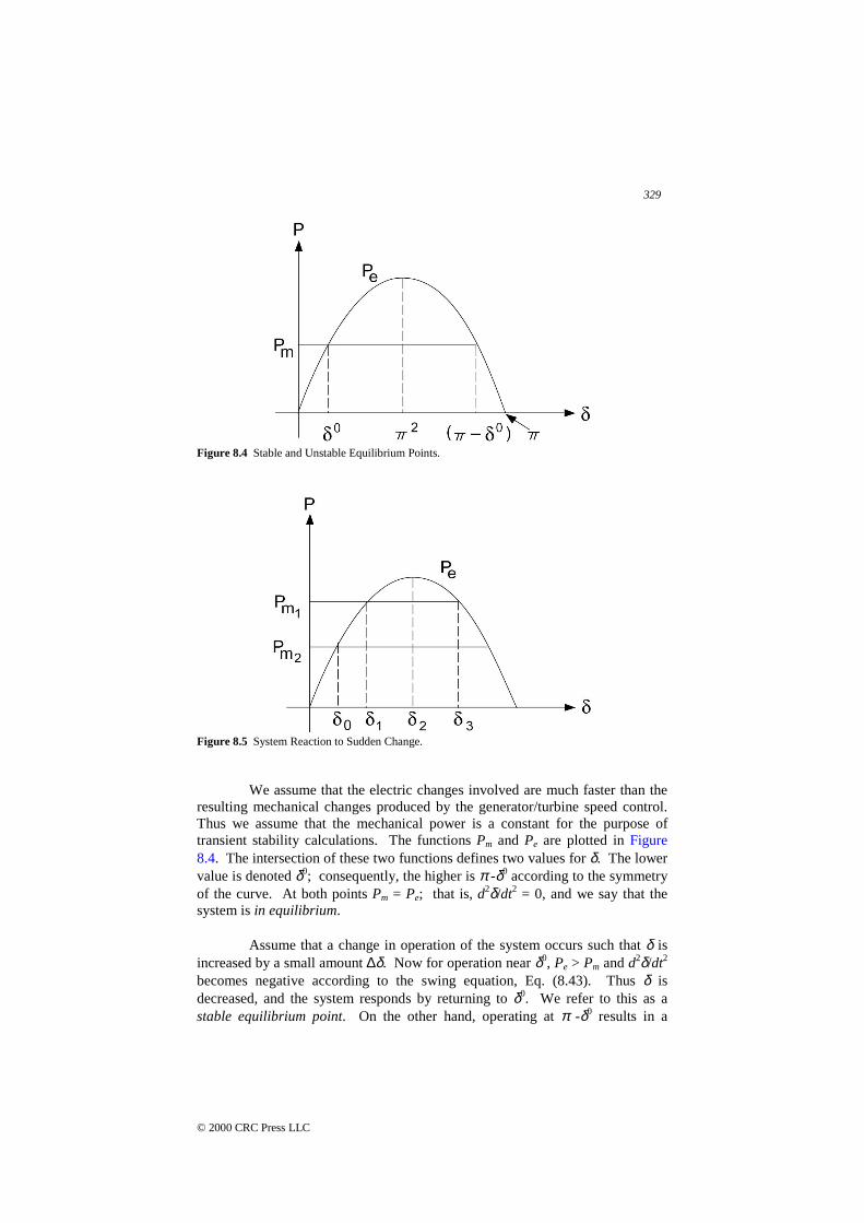
Figure 8.4 Stable and Unstable Equilibrium Points.

Figure 8.5 System Reaction to Sudden Change.

We assume that the electric changes involved are much faster than theresulting mechanical changes produced by the generator/turbine speed control.Thus we assume that the mechanical power is a constant for the purpose oftransient stability calculations. The functions Pm and Pe are plotted in Figure8.4. The intersection of these two functions defines two values for δ. The lowervalue is denoted δ0; consequently, the higher is π -δ0 according to the symmetryof the curve. At both points Pm = Pe; that is, d2δ/dt2 = 0, and we say that thesystem is in equilibrium.

Assume that a change in operation of the system occurs such that δ isincreased by a small amount ∆δ. Now for operation near δ0, Pe > Pm and d2δ/dt2

becomes negative according to the swing equation, Eq. (8.43). Thus δ isdecreased, and the system responds by returning to δ0. We refer to this as astable equilibrium point. On the other hand, operating at π -δ0 results in a

330


system response that will increase δ and moving further from π -δ0. For thisreason, we call π - δ0 an unstable equilibrium point.

If the system is operating in an equilibrium state supplying an electricpower

0eP with the corresponding mechanical power input 0mP , then

00 em PP =

and the corresponding rotor angle is δ0. Suppose the mechanical power Pm ischanged to

1mP at a fast rate, which the angle δ cannot follow as shown in

Figure 8.5. In this case, Pm > Pe and acceleration occurs so that δ increases.This goes on until the point δ1 where Pm = Pe, and the acceleration is zero. Thespeed, however, is not zero at that point, and δ continues to increase beyond δ1.In this region, Pm < Pe and rotor retardation takes place. The rotor will stop atδ2, where the speed is zero and retardation will bring δ down. This processcontinues on as oscillations around the new equilibrium point δ1. This serves toillustrate what happens when the system is subjected to a sudden change in thepower balance of the right-hand side of the swing equation.

Changes in the network configuration between the two sides (sendingand receiving) will alter the value of Xeq and hence the expression for the electricpower transfer. For example, opening one circuit of a double circuit lineincreases the equivalent reactance between the sending and receiving ends and

therefore reduces the maximum transfer capacity eqX

EV.

A Method for Stability Assessment

In order to predict whether a particular system is stable after adisturbance it is necessary to solve the dynamic equation describing the behaviorof the angle δ immediately following an imbalance or disturbance to the system.The system is said to be unstable if the angle between any two machines tends toincrease without limit. On the other hand, if under disturbance effects, theangles between every possible pair reach maximum value and decreasethereafter, the system is deemed stable.

Assuming as we have already done that the input is constant, withnegligible damping and constant source voltage behind the transient reactance,the angle between two machines either increases indefinitely or oscillates afterall disturbances have occurred. Therefore, in the case of two machines, the twomachines either fall out of step on the first swing or never. Here the observationthat the machines’ angular differences stay constant can be taken as anindication of system stability. A simple method for determining stability knownas the equal-area method is available, and is discussed in the following.

331


The Equal-Area Method

The swing equation for a machine connected to an infinite bus can bewritten as

M

P

dt

d a=ω(8.45)

where ω = dδ/dt and Pa is the accelerating power. We would like to obtain anexpression for the variation of the angular speed ω with Pa. We observe that Eq.(8.45) can be written in the alternate form

dtd

d

M

pd a

=

δδω

or

( )δωω dM

Pd a=

Integrating, we obtain

( )δωωδ

δ

ω

ωdP

Md a∫∫ =

00

1

Note that we may assume ω0 = 0; consequently,

( )δωδ

δdP

M a∫=0

22

or

( )21

0

2

= ∫

δ

δδδ

dPMdt

da (8.46)

The above equation gives the relative speed of the machine with respect to areference from moving at a constant speed (by the definition of the angle δ).

If the system is stable, then the speed must be zero when theacceleration is either zero or is opposing the rotor motion. Thus for a rotor thatis accelerating, the condition for stability is that a value of δs exists such that

( ) 0≤saP δ

332


and

( ) 00

=∫ δδ

δdP

s

a

This condition is applied graphically in Figure 8.6 where the net area under thePa - δ curve reaches zero at the angle δs as shown. Observe that at δs, Pa isnegative, and consequently the system is stable. Also observe that area A1

equals A2 as indicated.

The accelerating power need not be plotted to assess stability. Instead,the same information can be obtained form a plot of electrical and mechanicalpowers. The former is the power angle curve, and the latter is assumed constant.In this case, the integral may be interpreted as the area between the Pe curve andthe curve of Pm, both plotted versus δ. The area to be equal to zero must consistof a positive portion A1, for which Pm > Pe, and an equal and opposite negativepotion A2, for which Pm < Pe. This explains the term equal-area criterion fortransient stability. This situation is shown in Figure 8.7.

If the accelerating power reverses sign before the two areas A1 and A2

are equal, synchronism is lost. This situation is illustrated in Figure 8.8. Thearea A2 is smaller that A1, and as δ increases beyond the value where Pa reversessign again, the area A3 is added to A1.

Figure 8.6 The Equal-Area Criterion for Stability for a Stable System.

Figure 8.7 The Equal-Area Criterion for Stability.

333


Figure 8.8 The Equal-Area Criterion for an Unstable System.

Improving System Stability

The stability of the electric power system can be affected by changes inthe network or changes in the mechanical (steam or hydraulic) system. Networkchanges that adversely affect system stability ca either decrease the amplitude ofthe power curve or raise the load line. Examples of events that decrease theamplitude of the power curve are: short circuits on tie lines, connecting a shuntreactor, disconnecting a shunt capacitor, or opening a tie line. Events that raisethe load line include: disconnecting a resistive load in a sending area,connecting a resistive load in a receiving area, the sudden loss of a large load ina sending area, or the sudden loss of a generator in a receiving area. Changes ina steam or hydraulic system that can affect stability include raising the load lineby either closing valves or gates in receiving areas or opening valves or gates insending areas.

There are several corrective actions that can be taken in order toenhance the stability of the system following a disturbance. These measures canbe classified according to the type of disturbance – depending on whether it is aloss of generation or a loss of load.

In the case of a loss of load, the system will have an excess powersupply. Among the measures that can be taken are:

1. Resistor braking.2. Generator dropping.3. Initiation along with braking, fast steam valve closures, bypassing

of steam, or reduction of water acceptance for hydro units.

In the case of loss of generation, countermeasures are:

1. Load shedding.2. Fast control of valve opening in steam electric plants; and in the

case of hydro, increasing the water acceptance.

The measures mentioned above are taken at either the generation or the loadsides in the system. Measures that involve the interties (the lines) can be takento enhance the stability of the system. Among these we have the switching of

334


series capacitors into the lines, the switching of shunt capacitors or reactors, orthe boosting of power on HVDC lines.

Resistor braking relies on the connection of a bank of resistors in shuntwith the three-phase bus in a generation plant in a sending area through asuitable switch. This switch is normally open and will be closed only upon theactivation of a control device that detects the increase in kinetic energyexceeding a certain threshold. Resistive brakes have short time ratings to makethe cost much less than that of a continuous-duty resistor of the same rating. Ifthe clearing of the short circuit is delayed for more than the normal time (aboutthree cycles), the brakes should be disconnected and some generation should bedropped.

Generator dropping is used to counteract the loss of a large load in asending area. This is sometimes used as a cheap substitute for resistor brakingto counteract short circuits in sending systems. It should be noted that bettercontrol is achieved with resistor braking than with generator droppings.

To counteract the loss of generation, load shedding is employed. Inthis instance, a rapid opening of selected feeder circuit breakers in selected loadareas is arranged. This disconnects the customer’s premises with interruptibleloads such as heating, air conditioning, air compressors, pumps where storage isprovided in tanks, or reservoirs. Aluminum reduction plants are among loadsthat can be interrupted with only minor inconvenience. Load shedding bytemporary depression of voltage can also be employed. This reduction ofvoltage can be achieved either by an intentional short circuit or by theconnection of a shunt reactor.

The insertion of switched series capacitors can counteract faults on acinterties or permanent faults on dc interties in parallel with ac lines. In eithercase, the insertion of the switched series capacitor decreases the transferreactance between the sending and receiving ends of the interconnection andconsequently increases the amplitude of the sine curve and therefore enhancesthe stability of the system. It should be noted that the effect of a shunt capacitorinserted in the middle of the intertie or the switching off of a shunt reactor in themiddle of the intertie is equivalent to the insertion of a series capacitor (this canbe verified by means of a Y-∆ transformation).

To relieve ac lines of some of the overload and therefore provide alarger margin of stability, the power transfer on a dc line may be boosted. Thisis one of the major advantages of HVDC transmission.

8.6 POWER SYSTEM STATE ESTIMATION

Within the framework of an energy control center, there are three typesof real-time measurements:

335


• Analog measurements that include real and reactive power flowsthrough transmission lines, real and reactive power injections(generation or demand at buses), and bus voltage magnitudes.

• Logic measurements that consist of the status of switches/breakers,and transformer LTC positions.

• Pseudo-measurements that may include predicted bus loads andgeneration.

Analog and logic measurements are telemetered to the control center.Errors and noise may be contained in the data. Data errors are due to failures inmeasuring and telemetry equipment, noise in the communication system, anddelays in the transmission of data.

The state of a system is described by a set of variables, which at time t0

contains all information about the system, which allows us to determinecompletely the system behavior at a future time t1. A convenient choice is theselection of a minimum set of variables, thus defining a minimum, but sufficientset of state variables. Note that the state variables are not necessarily directlyaccessible, measurable, or observable. Since the system model used is based ona nodal representation, the choice of the state variables is rather obvious.Assuming that line impedances are known, the state variables are the voltagemagnitudes and angles. This follows because all other values can be uniquelydefined once the state values are known.

State estimation is a mathematical procedure to yield a description ofthe power system by computing the best estimate of the state variables (busvoltages and angles) of the power system based on the received noisy data.Once state variables are estimated, secondary quantities (e.g., line flows) canreadily be derived. The network topology module processes the logicmeasurements to determine the network configuration. The state estimatorprocesses the set of analog measurements to determine the system state; it alsouses data such as the network parameters (e.g., line impedance), networkconfiguration supplied by the network topology, and sometimes, pseudo-measurements. Since it not practical to make extensive measurements ofnetwork parameters in the field, manufacturers data and one line drawings areused to determine parameter values. This may then introduce another source oferror.

The mathematical formulation of the basic power system stateestimator assumes that the power system is static. Consider a system, which ischaracterized by n state variables, denoted by ix , with i = 1, …, n. Let m

measurements be available. The measurement vector is denoted z and the statevector is x. If the noise is denoted by v, then the relation between measurementsand states denoted by h is given by:

iii vxhz += )( (8.47)

336


or in compact form:

vxhz += )(

Let us linearize h(x), and we thus deal with:

vHxz += (8.48)

H is called the measurement matrix and is independent of the state variables.

There are many techniques for finding the best estimate of x, denotedby x̂ . We discuss the most popular approach based on the weighted leastsquares WLS concept. The method aims to minimize the deviations between themeasurements and the corresponding equations. This requires minimizing thefollowing objective function:

[ ]21

)()( xhzkxJ ii

m

i −=∑ (8.49)

We can demonstrate that the optimal estimates are obtained using thefollowing recursive equation:

[ ] [ ])(1

1 kT

kkT

kkk xhzWHWHHxx −+=−

+ (8.50)

This means that the state variables are successively approximatedcloser and closer to some value and a convergence criterion determines when theiteration is stopped. The matrix W is called the weighting matrix, and relates themeasurements individually to each other. The results are influenced by thechoice of the elements of W. If one chooses W = I, all measurements are ofequal quality.

Observability

If the number of measurements is sufficient and well-distributedgeographically, the state estimator will give an estimate of system state (i.e., thestate estimation equations are solvable). In this case, the network is said to beobservable. Observability depends on the number of measurements availableand their geographic distribution. Usually a measurement system is designed tobe observable for most operating conditions. Temporary unobservability maystill occur due to unexpected changes in network topology or failures in thetelecommunication systems.

Before applying state estimation in power system operation, we need toconduct an observability analysis study. The aim here is to ensure that thereenough real-time measurements to make state estimation possible. If not, weneed to determine where should additional meters be placed so that stateestimation is possible. Moreover, we need to determine how are the states of

337


these observable islands estimated, and how are additional pseudo-measurements included in the measurement set to make state estimationpossible. Finally, we need to be able to guarantee that the inclusion of theadditional pseudo-measurements will not contaminate the result of the stateestimation. Observability analysis includes observability testing, identificationof observable islands, and measurement placement.

Bad Data Detection and Identification

State estimation is formulated as a weighted least square error problem,and implicitly assumes that the errors are small. Large errors or bad dataoccasionally occur. The residual (the Weighted Least Square error) will be largeif bad data or structural error is present. Action is needed to detect the bad data;identify which measurements are bad; and to remove all bad data so that they donot corrupt the state estimates. Detecting bad data is based on techniques ofhypothesis testing to determine when the residual or the error is too large. Note,however, that a switch indicating other than its true position can cause largererror and hence we may end up discarding a valid analog reading. In practice, amajor benefit of state estimation is identifying bad data in the system.

Benefits of Implementing a State Estimator

Implementation of a state estimator establishes the following data:

• The correct impedance data for all modeled facilities. This mightseem to be information which should be readily available from thesystem plans of any given power system. Note, however, thatbetween the time a facility is planned and placed in service,distances for transmission lines change due to right-of-wayrealignment, or the assumed conductor configuration is changed, orthe conductor selected is not as assumed, etc. The net result is thatthe impedance according to the system plan may be up to 10percent off from the present actual values.

• The correct fixed tap position for all transformers in the modelednetwork.

• The correct load tap changing information for all modeled LoadTap Changing (LTC) transformers.

• The correct polarity of all MW and MVAR flow meters.• Detect bad meters as they go bad. As a result, more confidence is

established in the entire active meter set if meters are corrected asthey are detected to be bad.

• When an unusual event occurs, the active meter set can be believedbefore the power system security process has been rerun. Thissaves time for the system operators.

External Network Modeling

In an interconnected system, the responsibility of each energy control

338


center is to operate its own part of the system. A control center receivestelemetered real-time measurements of its own system; referred to as the internalsystem. Neighboring systems are called the external system. Any unmonitoredportions of the internal system such as distribution/sub-transmission networks orunmonitored substations must also be incorporated in the “external” mode. Dataexchange between utilities is often a difficult and sensitive issue, and thisimpacts the state estimation function. It is not always clear how much of theneighboring systems need to be measured for satisfactory performance of thestate estimator.

To determine the current status of the internal system using a stateestimator, it is not necessary to know more about the external system. It isimportant, however, to include the response of the external system in evaluatingthe consequence of various contingencies for security assessment. An externalmodel is constructed either on-line or off-line, or using a combination of both.This model can be a full or a reduced power flow model, or a combination ofboth. The external model is then attached to the internal system as the powerflow model to evaluate the response of the internal system to variouscontingencies. A reduced power flow model of the external system is called anexternal equivalent.

There may be portions of the transmission or sub-transmission systemfor which there is no direct telemetry. The choices are whether to neglect thisportion, or put it into an equivalent form. It is often practical to eliminate aportion of the network if its most direct through-path directly paralleling amodeled transmission path is ten times or more the impedance of the modeledpath. If, on the other hand, the step-down transformers to that portion are to bemonitored, then the underlying system must be at least modeled as an equivalentpath.

8.7 POWER SYSTEM SECURITY

By power system security, we understand a qualified absence of risk ofdisruption of continued system operation. Security may be defined from acontrol point of view as the probability of the system's operating point remainingin a viable state space, given the probabilities of changes in the system(contingencies) and its environment (weather, customer demands, etc.).Security can be defined in terms of how it is monitored or measured, as theability of a system to withstand without serious consequences any one of a pre-selected list of “credible” disturbances (“contingencies”). Conversely,insecurity at any point in time can be defined as the level of risk of disruption ofa system's continued operation.

Power systems are interconnected for improved economy andavailability of supplies across extensive areas. Small individual systems wouldbe individually more at risk, but widespread disruptions would not be possible.On the other hand, interconnections make widespread disruptions possible.

339


Operation of interconnected power systems demands nearly precisesynchronism in the rotational speed of many thousands of large interconnectedgenerating units, even as they are controlled to continuously follow significantchanges in customer demand. There is considerable rotational energy involved,and the result of any cascading loss of synchronism among major systemelements or subsystems can be disastrous. Regardless of changes in system loador sudden disconnection of equipment from the system, synchronized operationrequires proper functioning of machine governors, and that operating conditionsof all equipment remain within physical capabilities.

The risk of cascading outages still exists, despite improvements madesince the 1965 northeast blackout in the United States. Many factors increasethe risks involved in interconnected system operation:

• Wide swings in the costs of fuels result in significant changes inthe geographic patterns of generation relative to load. This leads totransmission of electric energy over longer distances in patternsother than those for which the transmission networks had beenoriginally designed.

• Rising costs due to inflation and increasing environmentalconcerns constrain any relief through further transmissionconstruction. Thus, transmission, as well as generation, must beoperated closer to design limits, with smaller safety (security)margins.

• Relaxation of energy regulation to permit sales of electric energyby independent power producers, together with increasing pressurefor essentially uncontrolled access to the bulk power transmissionnetwork.

Development of the Concept of Security

Prior to the 1965 Northeast blackout, system security was part ofreliability assured at the system planning stage by providing a strong system thatcould ride out any “credible” disturbances without serious disruption. It is nolonger economically feasible to design systems to this standard. At that time,power system operators made sure that sufficient spinning reserve was on line tocover unexpected load increases or potential loss of generation and to examinethe impact of removing a line or other apparatus for maintenance. Wheneverpossible, the operator attempted to maintain a desirable voltage profile bybalancing VARs in the system.

Security monitoring is perceived as that of monitoring, throughcontingency analysis, the conditional transition of the system into an emergencystate.

Two Perspectives of Security Assessment

There is a need to clarify the roles of security assessment in the

340


planning and real-time operation environments. The possible ambiguity is theresult of the shift of focus from that of system robustness designed at theplanning stage as part of reliability, to that of risk avoidance that is a matteroperators must deal with in real time. The planner is removed from the time-varying real world environment within which the system will ultimatelyfunction. The term “security” within a planning context refers to those aspectsof reliability analysis that deal with the ability of the system, as it is expected tobe constituted at some future time, to withstand unexpected losses of certainsystem components. Reliability has frequently been considered to consist ofadequacy and security. Adequacy is the ability to supply energy to satisfy loaddemand. Security is the ability to withstand sudden disturbances. Thisperspective overlooks the fact that the most reliable system will ultimatelyexperience periods of severe insecurity from the operator’s perspective. Systemoperations is concerned with security as it is constituted at the moment, with amiscellaneous variety of elements out for maintenance, repair, etc., and exposedto environmental conditions that may be very different from the normalconditions considered in system planning. In operations, systems nearly alwayshave less than their full complement of equipment in service. As a result, anoperator must often improvise to improve security in ways that are outside thehorizon of planners.

Security Assessment Defined

Security assessment involves using available data to estimate therelative security level of the system currently or at some near-term future state.Approaches to security assessment are classified as either direct or indirect.

• The direct approach: This approach evaluates the likelihood ofthe system operating point entering the emergency state. Itcalculates the probability that the power System State will movefrom normal state to emergency state, conditioned on its currentstate, projected load variations, and ambient conditions. It iscommon practice to assess security by analyzing a fixed set ofcontingencies. The system is declared as insecure if any memberof the set would result in transition to the emergency state. This isa limiting form of direct assessment, since it implies a probabilityof one of the system's being in the emergency state conditioned onthe occurrence of any of the defined contingencies.

• The indirect approach: Here a number of reserve margins aretracked relative to predetermined levels deemed adequate tomaintain system robustness vis-a-vis pre-selected potentialdisturbances. An indirect method of security assessment defines aset of system “security” variables that should be maintained withpredefined limits to provide adequate reserve margins.Appropriate variables might include, MW reserves, equipmentemergency ratings (line, transformer, etc.), or VAR reserves withindefined regions. The reserve margins to be maintained for each ofthe security variables could be determined by offline studies for an

341


appropriate number of conditions with due consideration to thedegree to which random events can change the security level of asystem in real time. Security assessment then would consist oftracking all such reserve margins relative to system conditions.

For a number of years, security concerns dealt with potential post-contingency line overloads and because line MW loading can be studiedeffectively by means of a linear system network model, it was possible to studythe effects of contingencies using linear participation or distribution factors.Once derived for a given system configuration, they could be applied withoutfurther power flow analysis to determine post-contingency line loading even, bysuperposition, for multiple contingencies. Such a computationally simplemethod of analysis made on-line contingency assessment practicable for“thermal security,” where reactive flows were not of concern.

More recently, post-contingency voltage behavior has become aprominent element in security assessment. Assessment of “voltage security” is acomplex process because the behavior of a system undergoing voltage collapsecannot be completely explained on the basis of static analysis alone.

Implications of Security

The trend towards reducing the costs associated with robust systemshas lead to heightened requirements of active security control. This necessitatesan increase in the responsibilities of the system operator. Accordingly, itrequires operator training and the development and provision of tools that willenable the operator to function effectively in the new environment.

Security Analysis

On-line security analysis and control involve the following threeingredients:

• Monitoring• Assessment• Control

The following framework relates the three modules:

Step 1. Security Monitoring: Identify whether the system is in thenormal state or not using real-time system measurements. If the systemis in an emergency state, go to step 4. If load has been lost, go to step5.

Step 2. Security Assessment: If the system is in the normal state,determine whether the system is secure or insecure with respect to a setof next contingencies.

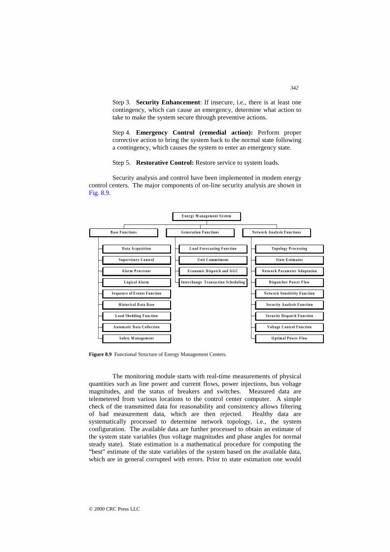
342


Step 3. Security Enhancement: If insecure, i.e., there is at least onecontingency, which can cause an emergency, determine what action totake to make the system secure through preventive actions.

Step 4. Emergency Control (remedial action): Perform propercorrective action to bring the system back to the normal state followinga contingency, which causes the system to enter an emergency state.

Step 5. Restorative Control: Restore service to system loads.

Security analysis and control have been implemented in modem energycontrol centers. The major components of on-line security analysis are shown inFig. 8.9.

D a ta A cq u isitio n

S u p e r viso r y C o n tr o l

A la r m P r oc e ssor

L o g ica l A la rm

S e q u e n c e o f E ve n ts F u n c tio n

H isto r ica l D a ta B a se

L o a d S h ed d in g F u n c tio n

A u to m a tic D a ta C o lle c t io n

S a fe ty M an a g e m e n t

B a se F u n c tio n s

L oa d F or e c astin g F u n c tio n

U n it C o m m itm en t

E co n o m ic D isp a tc h an d A G C

In ter c h a n g e T ra n sa c tio n S c h e d u lin g

G e n e ra tio n F u n ct ion s

To p o lo g y P r oc e ssin g

S ta te E stim a to r

N etw o r k P a ra m e te r A d a p ta tio n

D isp a tc h e r P o w e r F lo w

N etw o r k S en sitivity F u n c tio n

S e cu r ity A n a ly sis F u n ct io n

S e cu r ity D isp a tc h F u n c tio n

V olta ge C o n tro l F u n ct io n

O p tim a l P o w er F low

N etw o r k A n a ly sis F u n c tio n s

E n er g y M a n a g e m en t S y ste m

Figure 8.9 Functional Structure of Energy Management Centers.

The monitoring module starts with real-time measurements of physicalquantities such as line power and current flows, power injections, bus voltagemagnitudes, and the status of breakers and switches. Measured data aretelemetered from various locations to the control center computer. A simplecheck of the transmitted data for reasonability and consistency allows filteringof bad measurement data, which are then rejected. Healthy data aresystematically processed to determine network topology, i.e., the systemconfiguration. The available data are further processed to obtain an estimate ofthe system state variables (bus voltage magnitudes and phase angles for normalsteady state). State estimation is a mathematical procedure for computing the“best” estimate of the state variables of the system based on the available data,which are in general corrupted with errors. Prior to state estimation one would

343


like to know:

1) Whether state estimation of the system is possible (enough of thenetwork is observable), and if not, for which part of the systemstate estimation is still possible.

2) Whether there is any bad data present, and if so, which data is badand should be discarded.

Observability analysis and bad data detection and identification areparts of the state estimation function.

We need a set of contingencies to assess whether a normal operatingstate is secure or not. The contingency selection process employs a scheme toselect a set of important and plausible disturbances. Security assessmentinvolves primarily steady-state power flow analysis. Stability constraints areexpressed in terms of the limits on line flows and bus voltages. As a result, toassess system response to contingencies, a contingency evaluation is carried outusing on-line power flows. The on-line power flow uses the actual power flowmodel of the system under study (from the state estimation solution) togetherwith a system representation of the unmonitored network and neighboringsystems, i.e., an external network model.

Since the contingencies are future events, a bus-load forecast is needed.Certain implementations of the state estimator render the external modelobservable by strategic placement of pseudo-measurements. Then the stateestimate is performed on the entire model in one step.

8.8 CONTINGENCY ANALYSIS

Contingency analysis indicates to the operator what might happen tothe system in the event of unplanned equipment outage. It essentially offersanswers to questions such as “What will be the state of the system if an outageon part of the major transmission system takes place?” The answer might bethat power flows and voltages will readjust and remain within acceptable limits,or that severe overloads and under-voltages will occur with potentially severeconsequences should the outage take place.

A severe overload, persisting long enough, can damage equipment ofthe system, but usually relays are activated to isolate the affected equipmentonce it fails. The outage of a second component due to relay action is moreserious and often results in yet more readjustment of power flows and busvoltages. This can in turn cause more overloads and further removal ofequipment. An uncontrollable cascading series of overloads and equipmentremovals may then take place, resulting in the shutting down of a significantportion of the system.

The motivation to use contingency analysis tools in an EMS is thatwhen forewarned the operator can initiate preventive action before the event toavoid problems should an outage take place. From an economic point of view,

344


the operator strives to avoid overloads that might directly damage equipment, orworse, might cause the system to lose a number of components due to relayaction and then cause system-wide outages.

Insulation breakdown, over-temperature relay action, or simplyincorrect operation of relay devices is internal causes of contingencies. Externalcontingencies are caused by environmental effects such as lightning, high windsand ice conditions or else are related to some non-weather related events such asvehicle or aircraft coming into contact with equipment, or even human or animaldirect contact. These causes are treated as unscheduled, random events, whichthe operator can not anticipate, but for which they must be prepared.

The operators must play an active role in maintaining system security.The first step is to perform contingency analysis studies frequently enough toassure that system conditions have not changed significantly from the lastexecution. The outcome of contingency analysis is a series of warnings oralarms to the operators alerting them that loss of component A will result in anoverload of X% on line T1. To achieve an accurate picture of the system'sexposure to outage events several points need to be considered:

A) System Model

Contingency analysis is carried out using a power flow model of thesystem. Additional information about system dynamics are needed to assessstability as well. Voltage levels and the geographic extent to include in themodel are issues to be considered. In practice, all voltage levels that have anypossibility of connecting circuits in parallel with the high voltage system areincluded. This leaves out those that are radial to it such as distribution networks.While the geographical extent is difficult to evaluate, it is common to model thesystem to the extent real-time measurement data is available to support themodel.

B) Contingency Definition

Each modeled contingency has to be specified on its own. The simplestdefinition is to name a single component. This implies that when the model ofthe system is set up, this contingency will be modeled by removing the singlecomponent specified. Another important consideration is the means ofspecifying the component outage. The component can be specified by name,such as a transmission line name, or more accurately, a list of circuit breakerscan be specified as needing to be operated to correctly model the outage of thecomponent. Contingencies that require more than one component to be takenout together must be defined as well. There is an advantage here to using a “listof breakers” in that the list is simply expanded to include all breakers necessaryto remove all relevant equipment.C) Double Contingencies

A double contingency is the overlapping occurrence of two

345


independent contingent events. To be specific, one outside event causes anoutage and while this outage is still in effect, a second totally independent eventcauses another component to be taken out. The overlap of the two outages oftencauses overloads and under-voltages that would not occur if either happenedseparately. As a result, many operators require that a contingency analysisprogram be able to take two independent contingencies and model them as ifthey had happened in an overlapping manner.

D) Contingency List

Generally, contingency analysis programs are executed based a list ofvalid contingencies. The list might consist of all single component outagesincluding all transmission lines, transformers, substation buses, and all generatorunits. For a large interconnected power system just this list alone could result inthousands of contingency events to be tested. If the operators wished to modeldouble contingencies, the number becomes millions of possible events.Methods of selecting a limited set of priority contingencies are then needed.

E) Speed

Generally, operators need to have results from a contingency analysisprogram in the order of a few minutes up to fifteen minutes. Anything longermeans that the analysis is running on a system model that does not reflectcurrent system status and the results may not be meaningful.

F) Modeling Detail

The detail required for a contingency case is usually the same as thatused in a study power flow. That is, each contingency case requires a fullyconverged power flow that correctly models each generator's VAR limits andeach tap adjusting transformer's control of voltage.

Historical Methods of Contingency Analysis

There is a conflict between the accuracy with which the power systemis modeled and the speed required for modeling all the contingencies specifiedby the operator. If the contingencies can be evaluated fast enough, then all casesspecified on the contingency list are run periodically and alarms reported to theoperators. This is possible if the computation for each outage case can beperformed very fast or else the number of contingencies to be run is very small.The number of contingency cases to be solved in common energy managementsystems is usually a few hundred to a few thousand cases. This coupled with thefact that the results are to be as accurate as if run with a full power flow programmake the execution of a contingency analysis program within an acceptable timeframe extremely difficult.Selection of Contingencies to be Studied

A full power flow must be used to solve for the resulting flows and

346


voltages in a power system with serious reactive flow or voltage problems whenan outage occurs. In this case, the operators of large systems looking at a largenumber of contingency cases may not be able to get results soon enough. Asignificant speed increase could be obtained by simply studying only theimportant cases, since most outages do not cause overloads or under-voltages.

1) Fixed List

Many operators can identify important outage cases and they can getacceptable performance. The operator chooses the cases based on experienceand then builds a list for the contingency analysis program to use. It is possiblethat one of the cases that were assumed to be safe may present a problembecause some assumptions used in making the list are no longer true.

2) Indirect Methods (Sensitivity-Based Ranking Methods)

An alternative way to produce a reduced contingency list is to performa computation to indicate the possible bad cases and perform it as often as thecontingency analysis itself is run. This builds the list of cases dynamically andthe cases that are included in the list may change as conditions on the powersystem change. This requires a fast approximate evaluation to discover thoseoutage cases that might present a real problem and require further detailedevaluation by a full power flow. Normally, a sensitivity method based on theconcept of a network performance index is employed. The idea is to calculate ascalar index that reflects the loading on the entire system.

3) Comparison of Direct and Indirect Methods

Direct methods are more accurate and selective than the indirect ones atthe expense of increased CPU requirements. The challenge is to improve theefficiency of the direct methods without sacrificing their strengths. Directmethods assemble severity indices using monitored quantities (bus voltages,branch flows, and reactive generation), that have to be calculated first. Incontrast, the indirect methods calculate severity indices explicitly withoutevaluating the individual quantities. Therefore, indirect methods are usually lesscomputationally demanding. Knowing the individual monitored quantitiesenables one to calculate severity indices of any desired complexity withoutsignificantly affecting the numerical performance of direct methods. Therefore,more attention has been paid recently to direct methods for their superioraccuracy (selectivity). This has lead to drastic improvements in their efficiencyand reliability.

4) Fast Contingency Screening Methods

To build a reduced list of contingencies one uses a fast solution(normally an approximate one) and ranks the contingencies according to itsresults. Direct contingency screening methods can be classified by theimbedded modeling assumptions. Two distinct classes of methods can be

347


identified:

a) Linear methods specifically intended to screen contingenciesfor possible real power (branch MW overload) problems.

b) Nonlinear methods intended to detect both real and reactivepower problems (including voltage problems).

Bounding methods offer the best combination of numerical efficiencyand adaptability to system topology changes. These methods determine theparts of the network in which branch MW flow limit violations may occur. Alinear incremental solution is performed only for the selected system areas ratherthan for the entire network. The accuracy of the bounding methods is onlylimited by the accuracy of the incremental linear power flow.

Nonlinear methods are designed to screen the contingencies for reactivepower and voltage problems. They can also screen for branch flow problems(both MW and MVA/AMP). Recent proposed enhancements include attemptsto localize the outage effects, and speeding the nonlinear solution of the entiresystem.

An early localization method is the “concentric relaxation” whichsolves a small portion of the system in the vicinity of the contingency whiletreating the remainder of the network as an “infinite expanse.” The area to besolved is concentrically expanded until the incremental voltage changes alongthe last solved tier of buses are not significantly affected by the inclusion of anadditional tier of buses. The method suffered from unreliable convergence, lackof consistent criteria for the selection of buses to be included in the smallnetwork; and the need to solve a number of different systems of increasing sizeresulting from concentric expansion of the small network (relaxation).

Different attempts have been made at improving the efficiency of thelarge system solution. They can be classified as speed up the solution by meansof:

1) Approximations and/or partial (incomplete) solutions.2) Using network equivalents (reduced network representation).

The first approach involves the “single iteration” concept to takeadvantage of the speed and reasonably fast convergence of the Fast DecoupledPower Flow to limit the number of iterations to one. The approximate, firstiteration solution can be used to check for major limit violations and thecalculation of different contingency severity measures. The single iterationapproach can be combined with other techniques like the use of the reducednetwork representations to improve numerical efficiency.

An alternative approach is based upon bounding of outage effects.Similar to the bounding in linear contingency screening, an attempt is made toperform a solution only in the stressed areas of the system. A set of boundingquantities is created to identify buses that can potentially have large reactive

348


mismatches. The actual mismatches are then calculated and the forwardsolution is performed only for those with significant mismatches. All busvoltages are known following the backward substitution step and a number ofdifferent severity indices can be calculated.

The zero mismatch (ZM) method extends the application of localizationideas from contingency screening to full iterative simulation. Advantage istaken of the fact that most contingencies significantly affect only small portions(areas) of the system. Significant mismatches occur only in very few areas ofthe system being modeled. There is a definite pattern of very small mismatchesthroughout the rest of the system model. This is particularly true for localizablecontingencies, e.g., branch outages, bus section faults. Consequently, it shouldbe possible to utilize this knowledge and significantly speed up the solution ofsuch contingencies. The following is a framework for the approach:

1) Bound the outage effects for the first iteration using for example aversion of the complete boundary.

2) Determine the set of buses with significant mismatches resultingfrom angle and magnitude increments.

3) Calculate mismatches and solve for new increments.4) Repeat the last two steps until convergence occurs.

The main difference between the zero mismatch and the concentricrelaxation methods is in the network representation. The zero mismatch methoduses the complete network model while a small cutoff representation is used inthe latter one. The zero mismatch approach is highly reliable and producesresults of acceptable accuracy because of the accuracy of the networkrepresentation and the ability to expand the solution to any desired bus.

8.9 OPTIMAL PREVENTIVE AND CORRECTIVE ACTIONS

For contingencies found to cause overloads, voltage limit violations, orstability problems, preventive actions are required. If a feasible solution existsto a given security control problem, then it is highly likely that other feasiblesolutions exist as well. In this instance, one solution must be chosen fromamong the feasible candidates. If a feasible solution does not exist (which isalso common), a solution must be chosen from the infeasible candidates.Security optimization is a broad term to describe the process of selecting apreferred solution from a set of (feasible or infeasible) candidate solutions. Theterm Optimal Power Flow (OPF) is used to describe the computer applicationthat performs security optimization within an Energy Management System.

Optimization in Security Control

To address a given security problem, an operator will have more thanone control scheme. Not all schemes will be equally preferred and the operator

349


will thus have to choose the best or “optimal” control scheme. It is desirable tofind the control actions that represent the optimal balance between security,economy, and other operational considerations. The need is for an optimalsolution that takes all operational aspects into consideration. Securityoptimization programs may not have the capability to incorporate all operationalconsiderations into the solution, but this limitation does not prevent securityoptimization programs from being useful to utilities.

The solution of the security optimization program is called an “optimalsolution” if the control actions achieve the balance between security, economy,and other operational considerations. The main problem of securityoptimization seeks to distinguish the preferred of two possible solutions. Amethod that chooses correctly between any given pair of candidate solutions iscapable of finding the optimal solution out of the set of all possible solutions.There are two categories of methods for distinguishing between candidatesolutions: one class relies on an objective function, the other class relies onrules.

1) The Objective Function

The objective function method assumes that it is possible to assign asingle numerical value to each possible solution, and that the solution with thelowest value is the optimal solution. The objective function is this numericalassignment. In general, the objective function value is an explicit function ofthe controls and state variables, for all the networks in the problem.Optimization methods that use an objective function typically exploit itsanalytical properties, solving for control actions that represent the minimum.The conventional optimal power flow (OPF) is an example of an optimizationmethod that uses an objective function.

The advantages of using an objective function method are:

• Analytical expressions can be found to represent MW productioncosts and transmission losses, which are, at least from an economicview point, desirable quantities to minimize.

• The objective function imparts a value to every possible solution.Thus all candidate solutions can, in principle, be compared on thebasis of their objective function value.

• The objective function method assures that the optimal solution ofthe moment can be recognized by virtue of its having the minimumvalue.

Typical objective functions used in OPF include MW production costsor expressions for active (or reactive) power transmission losses. However,when the OPF is used to generate control strategies that are intended to keep thepower system secure, it is typical for the objective function to be an expressionof the MW production costs, augmented with fictitious control costs thatrepresent other operational considerations. This is especially the case when

350


security against contingencies is part of the problem definition. Thus whensecurity constrained OPF is implemented to support real-time operations, theobjective function tends to be a device whose purpose is to guide the OPF tofind the solution that is optimal from an operational perspective, rather than onewhich represents a quantity to be minimized.

Some examples of non-economic operational considerations that autility might put into its objective function are:

• a preference for a small number of control actions;• a preference to keep a control away from its limit;• the relative preference or reluctance for preventive versus post-

contingent action when treating contingencies; and• a preference for tolerating small constraint violations rather than

taking control action.

The most significant shortcoming of the objective function method isthat it is difficult (sometimes impossible) to establish an objective function thatconsistently reflects true production costs and other non-economic operationalconsiderations.

2) Rules

Rules are used in methods relying on expert systems techniques. Arule-based method is appropriate when it is possible to specify rules forchoosing between candidate solutions easier than by modeling these choices viaan objective function. Optimization methods that use rules typically search for arule that matches the problem addressed. The rule indicates the appropriatedecision (e.g., control action) for the situation. The main weakness of a rule-based approach is that the rule base does not provide a continuum in the solutionspace. Therefore, it may be difficult to offer guidance for the OPF from the rulebase when the predefined situations do not exist in the present power systemstate.

Rules can play another important role when the OPF is used in the real-time environment. The real-time OPF problem definition itself can be illdefined and rules may be used to adapt the OPF problem definition to thecurrent state of the power system.

Optimization Subject to Security Constraints

The conventional OPF formulation seeks to minimize an objectivefunction subject to security constraints, often presented as “hard constraints,” forwhich even small violations are not acceptable. A purely analytical formulationmight not always lead to solutions that are optimal from an operationalperspective. Therefore, the OPF formulation should be regarded as a frameworkin which to understand and discuss security optimization problems, rather thanas a fundamental representation of the problem itself.

351


1) Security Optimization for the Base Case State

Consider the security optimization problem for the base case stateignoring contingencies. The power system is considered secure if there are noconstraint violations in the base case state. Thus any control action required willbe corrective action. The aim of the OPF is to find the optimal corrective action.

When the objective function is defined to be the MW production costs,the problem becomes the classical active and reactive power constraineddispatch. When the objective function is defined to be the active powertransmission losses, the problem becomes one of active power lossminimization.

2) Security Optimization for Base Case and Contingency States

Now consider the security optimization problem for the base case andcontingency states. The power system is considered secure if there are noconstraint violations in the base case state, and all contingencies are manageablewith post-contingent control action. In general, this means that base case controlaction will be a combination of corrective and preventive actions and that post-contingent control action will be provided in a set of contingency plans. Theaim of the OPF is then to find the set of base case control actions pluscontingency plans that is optimal.

Dealing with contingencies requires solving OPF involving multiplenetworks, consisting of the base case network and each contingency network.To obtain an optimal solution, these individual network problems must beformulated as a multiple network problem and solved in an integrated fashion.The integrated solution is needed because any base case control action willaffect all contingency states, and the more a given contingency can be addressedwith post-contingency control action, the less preventive action is needed forthat contingency.

When an operator is not willing to take preventive action, then allcontingencies must be addressed with post-contingent control action. Theabsence of base case control action decouples the multiple network problemsinto a single network problem for each contingency. When an operator is notwilling to rely on post-contingency control action, then all contingencies mustbe addressed with preventive action. In this instance, the cost of the preventiveaction is preferred over the risk of having to take control action in the post-contingency state. The absence of post-contingency control action means thatthe multiple network problem may be represented as the single network problemfor the base case, augmented with post-contingent constraints.

Security optimization for base case and contingency states will involvebase case corrective and preventive action, as well as contingency plans forpost-contingency action. To facilitate finding the optimal solution, the objective

352


function and rules that reflect operating policy are required. For example, if it ispreferred to address contingencies with post-contingency action rather thanpreventive action, then post-contingent controls may be modeled as having alower cost in the objective function. Similarly, a preference for preventiveaction over contingency plans could be modeled by assigning the post-contingent controls a higher cost than the base case controls. Somecontingencies are best addressed with post-contingent network switching. Thiscan be modeled as a rule that for a given contingency, switching is to beconsidered before other post-contingency controls.

3) Soft Constraints

Another form of security optimization involves “soft” securityconstraints that may be violated but at the cost of incurring a penalty. This is amore sophisticated method that allows a true security/economy trade-off. Itsdisadvantage is requiring a modeling of the penalty function consistent with theobjective function. When a feasible solution is not possible, this is perhaps thebest way to guide the algorithm toward finding an “optimal infeasible” solution.

4) Security versus Economy

As a general rule, economy must be compromised for security.However, in some cases security can be traded off for economy. If theconstraint violations are small enough, it may be preferable to tolerate them inreturn for not having to make the control moves. Many constraint limits are nottruly rigid and can be relaxed. Thus, in general, the security optimizationproblem seeks to determine the proper balance of security and economy. Whensecurity and economy are treated on the same basis, it is necessary to have ameasure of the relative value of a secure, expensive state relative to a lesssecure, but also less expensive state.

5) Infeasibility

If a secure state cannot be achieved, there is still a need for the leastinsecure operating point. For OPF, this means that when a feasible solutioncannot be found, it is still important that OPF reach a solution, and that thissolution be “optimal” in some sense, even though it is infeasible. This isespecially appropriate for OPF problems that include contingencies in theirdefinition. The OPF program needs to be capable of obtaining the “optimalinfeasible” solution. There are several approaches to this problem. Perhaps thebest approach is one that allows the user to model the relative importance ofspecific violations, with this modeling then reflected in the OPF solution. Thismodeling may involve the objective function (i.e., penalty function) or rules, orboth.The Time Variable

The preceding discussion assumes that all network states are based onthe same (constant) frequency, and all transient effects due to switching andoutages are assumed to have died out. While bus voltages and branch flows are,

353


in general, sinusoidal functions of time, only the amplitudes and phaserelationships are used to describe network state. Load, generation, andinterchange schedules change slowly with time, but are treated as constant in thesteady state approximation. There are still some aspects of the time variable thatneed to be accounted for in the security optimization problem.

1) Time Restrictions on Violations and Controls

The limited amount of time to correct constraint violations is a securityconcern. This is because branch flow thermal limits typically have severallevels of rating (normal, emergency, etc.), each with its maximum time ofviolation. (The higher the rating, the shorter the maximum time of violation.)Voltage limits have a similar rating structure and there is very little time torecover from a violation of an emergency voltage rating.

Constraint violations need to be corrected within a specific amount oftime. This applies to violations in contingency states as well as actual violationsin the base case state. Base case violations, however, have the addedseriousness of the elapsed time of violation: a constraint that has been violatedfor a period of time has less time to be corrected than a constraint that has justgone into violation.

The situation is further complicated by the fact that controls cannotmove instantaneously. For some controls, the time required for movement issignificant. Generator ramp rates can restrict the speed with which active poweris rerouted in the network. Delay times for switching capacitors and reactorsand transformer tap changing mechanisms can preclude the immediatecorrection of serious voltage violations. If the violation is severe enough, slowcontrols that would otherwise be preferred may be rejected in favor of fast, lesspreferred controls. When the violation is in the contingency state, the timecriticality may require the solution to chose preventive action even though acontingency plan for post-contingent corrective action might have been possiblefor a less severe violation.

2) Time in the Objective Function

It is common for the MW production costs to dominate the character ofthe objective function for OPF users. The objective function involves the timevariable to the extent that the OPF is minimizing a time rate of change. This isalso the case when the OPF is used to minimize the cost of imported power oractive power transmission losses. Not all controls in the OPF can be “costs” interms of dollars per hour. The start-up cost for a combustion turbine, forexample, is expressed in dollars, not dollars per hour. The costing of reactivecontrols is even more difficult, since the unwillingness to move these controls isnot easily expressed in either dollars or dollars per hour. OPF technologyrequires a single objective function, which means that all control costs must beexpressed in the same units. There are two approaches to this problem:

354


• Convert dollar per hour costs into dollar costs by specifying a timeinterval for which the optimization is to be valid. Thus controlcosts in dollars per hour multiplied by the time interval, yieldcontrol costs in dollars. This is now in the same units as controlswhose costs are “naturally” in dollars. This approach thus“integrates” the time variable out of the objective functioncompletely. This may be appropriate when the OPF solution isintended for a well-defined (finite) period of time.

• Regard all fixed control costs (expressed in dollars) as occurringrepeatedly in time and thus having a justified conversion intodollars per hour. For example, the expected number of times peryear that a combustion turbine is started defines a cost per unittime for the start-up of the unit. Similarly, the unwillingness tomove reactive controls can be thought of as reluctance over andabove an acceptable amount of movement per year. This approachmay be appropriate when the OPF is used to optimize over arelatively long period of time.

• Simply adjust the objective function empirically so that the OPFprovides acceptable solutions. This method can be regarded as anexample of either of the first two approaches.

Using an Optimal Power Flow Program

OPF programs are used both in on-line and in off-line (study mode)studies. The two modes are not the same.

1) On-line Optimal Power Flow

The solution speed of an on-line OPF should be high enough so that theprogram completes before the power system configuration has changedappreciably. Thus the on-line OPF should be fast enough to run several time perhour. The values of the algorithm’s input parameters should be valid over awide range of operating states, such that the program continues to function asthe state of the system changes. Moreover, the application needs to address thecorrect security optimization problem and that the solutions conform to currentoperating policy.

2) Advisory Mode versus Closed Loop Control

On-line OPF programs are implemented in either advisory or closedloop mode. In advisory mode, the control actions that constitute the OPFsolution are presented as recommendations to the operator. For closed loopOPF, the control actions are actually implemented in the power system, typicallyvia the SCADA subsystem of the Energy Management System. The advisorymode is appropriate when the control actions need review by the dispatcherbefore their implementation. Closed loop control for security optimization isappropriate for problems that are so well defined that dispatcher review of thecontrol actions is not necessary. An example of closed loop on-line OPF is the

355


Constrained Economic Dispatch (CED) function. Here, the constraints are theactive power flows on transmission lines, and the controls are the MW output ofgenerators on automatic generation control (AGC). When the conventionalEconomic Dispatch would otherwise tend to overload the transmission lines inits effort to minimize production costs, the CED function supplies a correctionto the controls to avoid the overloads. Security optimization programs thatinclude active and reactive power constraints and controls, in contingency statesas well as in the base case, are implemented in an advisory mode. Thus theresults of the on-line OPF are communicated to the dispatchers via EMSdisplays. Considering the typical demands on the dispatchers’ time andattention in the control center, the user interface for on-line OPF needs to bedesigned such that the relevant information is communicated to the dispatchers“at-a-glance.”

3) Defining the Real-time Security Optimization Problem

As the power system state changes through time, the various aspects ofthe security optimization problem definition can change their relativeimportance. For example, concern for security against contingencies may be afunction of how secure the base case is. If the base case state has seriousconstraint violations, one may prefer to concentrate on corrective action alone,ignoring the risk of contingencies. In addition, the optimal balance of securityand economy may depend on the current security state of the power system.During times of emergency, cost may play little or no role in determining theoptimal control action. Thus the security optimization problem definition itselfcan be dynamic and sometimes ill defined.

8.10 DYNAMIC SECURITY ANALYSIS

The North American Electric Reliability Council (NERC) definessecurity as “the prevention of cascading outages when the bulk power supply issubjected to severe disturbances.” To assure that cascading outages will nottake place, the power system is planned and operated such that the followingconditions are met at all times in the bulk power supply:

• No equipment or transmission circuits are overloaded;• No buses are outside the permissible voltage limits (usually within

+5 percent of nominal); and• When any of a specified set of disturbances occurs, acceptable

steady-state conditions will result following the transient (i.e.,instability will not occur).

Security analysis is carried out to ensure that these conditions are met.The first two require only steady-state analysis; but the third requires transientanalysis (e.g., using a transient stability application). It has also been recognizedthat some of the voltage instability phenomena are dynamic in nature, andrequire new analysis tools.

356


Generally, security analysis is concerned with the system's response todisturbances. In steady-state analysis the transition to a new operating conditionis assumed to have taken place, and the analysis ascertains that operatingconstraints are met in this condition (thermal, voltage, etc.). In dynamic securityanalysis the transition itself is of interest, i.e., the analysis checks that thetransition will lead to an acceptable operating condition. Examples of possibleconcern include loss of synchronism by some generators, transient voltage at akey bus (e.g., a sensitive load) failing below a certain level and operation of anout-of-step relay resulting in the opening of a heavily loaded tie-line.

The computational capability of some control centers may limitsecurity analysis to steady state calculations. The post-contingency steady-stateconditions are computed and limit checked for flow or voltage violations. Thedynamics of the system may then be ignored and whether the post-contingencystate was reached without losing synchronism in any part of the system remainsunknown. As a result, instead of considering actual disturbances, thecontingencies are defined in terms of outages of equipment and steady-stateanalysis is done for these outages. This assumes that the disturbance did notcause any instability and that simple protective relaying caused the outage.Normally, any loss of synchronism will cause additional outages thus makingthe present steady-state analysis of the post-contingency condition inadequatefor unstable cases. It is clear that dynamic analysis is needed.

In practice, we define a list of equipment losses for static analysis.Such a list usually consists of all single outages and a careful choice of multipleoutages. Ideally, the outages should be chosen according to their probability ofoccurrence but these probabilities are usually not known. In some instance theavailable probabilities are so small that comparisons are usually meaningless.The choice of single outages is reasonable because they are likely to occur moreoften than multiple ones. Including some multiple outages is needed becausecertain outages are likely to occur together because of proximity (e.g., doublelines on the same tower) or because of protection schemes (e.g., a generator maybe relayed out when a line is on outage). The size of this list is usually severalhundred and can be a couple of thousand.

For dynamic security analysis, contingencies are considered in terms ofthe total disturbance. All faults can be represented as three phase faults, with orwithout impedances, and the list of contingencies is a list of locations where thiscan take place. This is a different way of looking at contingencies where thepost-contingency outages are determined by the dynamics of the systemincluding the protection system. Obviously, if all possible locations areconsidered, this list can be very large.

In steady-state security analysis, it is not necessary to treat all of thehundreds of outages cases using power flow calculations, because the operator isinterested in worst possibilities rather than all possibilities. It is practical to usesome approximate but faster calculations to filter out these worst outages, whichcan then be analyzed by a power flow. This screening of several hundred

357


outages to find the few tens of the worst ones has been the major breakthroughthat made steady state security analysis feasible. Generally, this contingencyscreening is done for the very large list of single outages while the multipleoutages are generally included in the short list for full power flow analysis.Currently, the trend is to use several different filters (voltage filter versus lineoverload filter) for contingency screening. It is also necessary to develop fastfiltering schemes for dynamic security analysis to find the few tens of worstdisturbances for which detailed dynamic analysis will have to be done. Thefilters are substantially different from those used for static security.

From a dispatcher’s point of view, static and dynamic security analysesare closely related. The worst disturbances and their effects on the system are tobe examined. The effects considered include the resulting outages and the limitviolations in the post-contingency condition. In addition, it would be useful toknow the mechanism that caused the outages, whether they were due to distancerelay settings or loss of synchronism or other reasons. This latter information isparticularly useful for preventive action.

The stability mechanism that causes the outages is referred to as the“mode of disturbance.” A number of modes exist. A single generating unit maygo out of synchronism on the first swing (cycle). A single unit may losesynchronism after several cycles, up to a few seconds. Relays may operate tocause transmission line outages. Finally, periodic oscillations may occurbetween large areas of load and/or generation. These oscillations may continueundamped to a point of loss of synchronism. All of these types of events arecalled modes of disturbances.

Motivation for Dynamic Security Analysis

Ascertaining power system security involves considering all possible(and credible) conditions and scenarios; analysis is then performed on all ofthem to determine the security limits for these conditions. The results are givento the operating personnel in the form of “operating guides,” establishing the“safe” regimes of operation. The key power system parameter or quantity ismonitored (in real time) and compared with the available (usually pre-computed) limit. If the monitored quantity is outside the limit, the situation isalerted or flagged for some corrective action.

Recent trends in operating power systems close to their security limits(thermal, voltage and stability) have added greatly to the burden on transmissionfacilities and increased the reliance on control. Simultaneously, they haveincreased the need for on-line dynamic security analysis.

For on-line dynamic security analysis, what is given is a base casesteady-state solution (the real time conditions as obtained from the stateestimator and external model computation, or a study case as set up by theoperator) and a list of fault locations. The effects of these faults have to bedetermined and, specifically, the expected outages have to be identified.

358


Examining the dynamic behavior of the system can do this. Some form of fastapproximate screening is required such that the few tens of worst disturbancescan be determined quickly.

Traditionally, for off-line studies, a transient stability program is usedto examine the dynamic behavior. This program, in the very least, models thedynamic behavior of the machines together with their interconnection throughthe electrical network. Most production grade programs have elaborate modelsfor the machines and their controls together with dynamic models of othercomponents like loads, dc lines, static VAR compensators, etc. These modelsare simulated in time using some integration algorithm and the dynamicbehavior of the system can be studied. If instability (loss of synchronism) isdetected, the exact mode of instability (the separation boundary) can beidentified. Many programs have relay models that can also pinpoint the outagescaused by relay operation due to the dynamic behavior.

To perform the analysis in on-line mode the time required for thecomputation is a crucial consideration. That is, the analysis itself by a pure timedomain simulation is known to be feasible but whether this analysis can becompleted within the time frame needed in the control center environment is thereal challenge. The time taken for time domain analysis of power systemdynamics depends on many factors. The most obvious one is the length ofsimulation or the time period for which the simulation needs to be done so thatall the significant effects of the disturbance can be captured. Other factorsinclude the size of the power system, and the size and type of the models used.Additional factors like the severity of the disturbance and the solution algorithmused also effects the computation time.

Determining the vulnerability of the present system conditions todisturbances does not complete the picture because the solution to any existingproblems must also be found. Quite often the post-contingency overloads andout-of limit voltage conditions are such that they can be corrected after theoccurrence of the fault. Sometimes, and especially for unstable faults, the post-contingency condition is not at all desirable and preventive remedial action isneeded. This usually means finding new limits for operating conditions orarming of special protective devices. Although remedial action is considered, asa separate function from security analysis, operators of stability limited systemsneed both.

Approaches to DSA

A number of approaches to the on-line dynamic stability analysisproblem have been studied. To date, engineers perform a large number ofstudies off-line to establish operating guidelines, modified by judgement andexperience. Conventional wisdom has it that computer capability will continueto make it more economically feasible to do on-line dynamic securityassessment, DSA, providing the appropriate methods are developed.

359


The most obvious method for on-line DSA is to implement the off-linetime domain techniques on faster, more powerful and cheaper computers.Equivalencing and localization techniques are ways to speed up the time domainsolutions. Also parallel and array processors show promise in acceleratingportions of the time domain solution.

Direct methods of transient stability, e.g., the transient energy functionmethod, have emerged with the potential of meeting some of the needs for DSA.They offer the possibility of conducting stability studies in near real-time,provide a qualitative judgement on stability, and they are suitable for use insensitivity assessments. The TEF methods are limited to first swing analysis.An advantage, however, is that the TEF methods provide energy margins toindicate the margin to instability.

Eigenvalue and related methods, and frequency response methods areused as part of off-line studies, for example, using frequency response method todesign power system stabilizers, but are not currently thought of as part of anon-line DSA. Probabilistic methods have the advantage of providing a measureof the likelihood of a stability problem. Their application in dynamic securityassessment appears to be in the areas of contingency screening and inquantifying the probability of the next state of the system.

Artificial intelligence techniques including computational neuralnetworks, fuzzy logic, and expert systems have proven to be appropriatesolutions to other power system operations problems, and there is speculationthat these technologies will play a major role in DSA.

electrical energy systems - erdinç kuruoğlu · electrical energy systems. series ed. ... reserves...

Documents