electrical resistivity imaging of the architecture of

Electrical resistivity imaging of the architecture

of substream sediments

N. Crook,1 A. Binley,2 R. Knight,1 D. A. Robinson,1,3 J. Zarnetske,4 and R. Haggerty4

Received 1 March 2008; revised 12 August 2008; accepted 3 September 2008; published 9 December 2008.

[1] The modeling of fluvial systems is constrained by a lack of spatial information aboutthe continuity and structure of streambed sediments. There are few methods fornoninvasive characterization of streambeds. Invasive methods using wells and cores fail toprovide detailed spatial information on the prevailing architecture and its continuity.Geophysical techniques play a pivotal role in providing spatial information on subsurfaceproperties and processes across many other environments, and we have applied the useof one of those techniques to streambeds. We demonstrate, through two examples,how electrical resistivity imaging can be utilized for characterization of subchannelarchitecture. In the first example, electrodes installed in riparian boreholes and on thestreambed are used for imaging, under the river bed, the thickness and continuity of ahighly permeable alluvial gravel layer overlying chalk. In the second example, electricalresistivity images, determined from data collected using electrodes installed on theriver bed, provide a constrained estimate of the sediment volume behind a log jam, vital tomodeling biogeochemical exchange, which had eluded measurement usingconventional drilling methods owing to the boulder content of the stream. The twoexamples show that noninvasive electrical resistivity imaging is possible in complexstream environments and provides valuable information about the subsurface architecturebeneath the stream channels.

Citation: Crook, N., A. Binley, R. Knight, D. A. Robinson, J. Zarnetske, and R. Haggerty (2008), Electrical resistivity imaging of the

architecture of substream sediments, Water Resour. Res., 44, W00D13, doi:10.1029/2008WR006968.

1. Introduction

[2] One of the challenges in studying rivers and streamsis quantification of the subsurface properties. At most sites,information about subsurface properties and processes hasbeen obtained using wells or trenches. Wells and trenchesare spatially limited and often cannot be installed more thana meter or two because site access prevents the use of largedrilling/coring equipment [e.g., Wondzell, 2006; Burkholderet al., 2008]. Given the pervasive spatial and temporalheterogeneity of the subsurface, however, such localizedmeasurements cannot provide the density of sampling(spatial or temporal) required to accurately characterizesubsurface properties and processes. In order to addressthe need for improved forms of subsurface measurement,geophysical techniques are increasingly applied to non-invasively sample or ‘‘image’’ subsurface regions. Thesegeophysical techniques can provide a means of obtaininginformation about the subsurface that cannot be acquiredthrough other, existing forms of measurement.

[3] One of the critical elements in many hydrologicsystems is the dynamic exchange between surface waterand groundwater along the bed of rivers and streams, in thehyporheic zone. The movements of water within the hypo-rheic zone are key regulators of head and nutrients in manyriverine ecosystems [Jones and Mulholland, 1999]. Studiesof the processes operating in this zone currently rely on thedirect sampling of the surface water chemistry, installationof shallow wells, use of natural and artificial tracers, andtesting of hydraulic properties, either in situ or from coresamples. What cannot be readily obtained from thesemeasurements is an accurate ‘‘image’’ of the large-scalearchitecture of the streambed materials through which thesurface water-groundwater exchange takes place. Combin-ing geophysical investigations with the traditional methodshighlighted can provide better informed subsurface charac-terizations together with information on subsurface processes.We demonstrate, in examples from the United Kingdom andthe United States, the usefulness of the geophysical techniquereferred to as electrical resistivity imaging (sometimes alsoreferred to as electrical resistivity tomography) to obtainhigh-resolution images of these underlying materials. Thisapplication of geophysical imaging provides an importantnew approach to characterize a critical region at the interfacebetween surface water and groundwater.[4] Electrical resistivity imaging (ERI) uses electrodes

located on the surface or in boreholes/wells to obtain animage of the electrical properties of a subsurface region. InERI, current is injected between two electrodes and poten-tial measurements are made at a number of other electrode

1Department of Geophysics, Stanford University, Stanford, California,USA.

2Lancaster Environment Centre, Lancaster University, Lancaster, UK.3Now at Department of Food Production, University of West Indies, St.

Augustine, Trinidad and Tobago.4Department of Geosciences, Oregon State University, Corvallis,

Oregon, USA.

Copyright 2008 by the American Geophysical Union.0043-1397/08/2008WR006968

W00D13

WATER RESOURCES RESEARCH, VOL. 44, W00D13, doi:10.1029/2008WR006968, 2008

1 of 11

pairs. This is repeated many times using multiple combina-tions of tens or hundreds of electrode pairs. These data areinverted to determine a model that best represents thesubsurface electrical resistivity structure. A more detailedexplanation of ERI theory and methodology can be found inthe work of Binley and Kemna [2005]. For our modeling inthe examples here we use a triangular finite element-basedforward solution coupled with an ‘‘Occam’s’’ style inver-sion [e.g., Constable et al., 1987]. The use of an ‘‘Occam’s’’style inversion produces a smooth model that fits a data setwithin certain tolerances. The model allows specification ofelectrode locations at any node within the finite elementmesh. Thus, as is the case in the following examples, theeffect of conductive features such as a water columncovering a number of the electrode locations can be incor-porated into the inversion.[5] The final product, a 2-D or 3-D resistivity image, is

interpreted using information about the link between theelectrical resistivity and subsurface material properties. ERIhas been used for a wide range of applications in hydrology,by taking advantage of the link between the estimatedgeophysical property, electrical resistivity, and materialproperties such as clay content, water content, and salinity.Hydrological examples include monitoring flow and trans-port in the vadose zone [e.g., Daily et al., 1992; al Hagreyand Michaelsen, 1999]; tracking tracer migration in thesaturated zone [e.g., Kemna et al., 2002; Singha andGorelick, 2005]; estimation of hydraulic properties [Binleyet al., 2002; Singha et al., 2007].[6] The objective of our research was to build on recent

ERI advancements to demonstrate its use as a means ofdetermining the geometry of sediment packages underly-ing streambeds. Imaging the subchannel sediment archi-tecture presents a departure from the typical electricalresistivity surveys, in that the electrodes need to besubmerged within the stream water column or physicallyembedded in the saturated streambed sediments. A recentadvance in ERI equipment, for waterborne surveys,includes the use of streamer resistivity techniques. Typi-cally this involves towing an array of electrodes after avessel, suspended in the water column using a series offloats. With the available resistivity systems, the first twoelectrodes are used as the current dipole, with the remain-ing electrodes making up the receiver dipoles (currenttechnology allows for between 2 and, typically, 10 receiverdipoles). Electrical measurements are taken continuouslytogether with GPS and sonar measurements, for the electrodepositions and water depth respectively. Applications of thisERI streamer technology include mapping submarinegroundwater discharge in estuarine environments [Day-Lewis et al., 2006; Breier et al., 2005; Manheim et al.,2004]; monitoring the discharge of nitrate-containinggroundwater into the marine environment [Andersen et al.,2007]; and delineation of faults beneath riverbeds [Kwon etal., 2005].[7] In some cases, electrodes may be deployed in bore-

holes, thus allowing higher-resolution of subsurface struc-tures at depth. This approach has been demonstrated ingroundwater studies [e.g., Slater et al., 1997; Kemna et al.,2004]. Acworth and Dasey [2003] have also shown poten-tial use of such deployment for groundwater-surface waterinteraction studies.

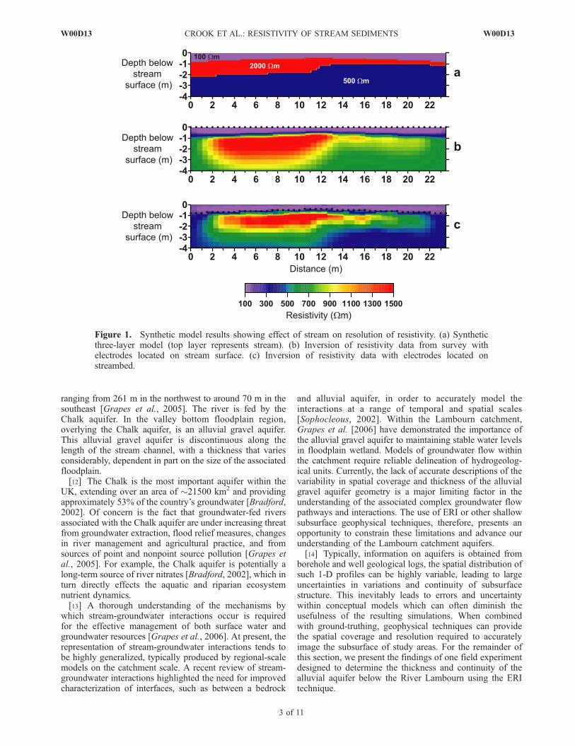
[8] Another deployment technique, which has receivedlittle attention in the literature, is the emplacement of theelectrodes directly in the streambed. In many watersheds theabove streamer technique would be unfeasible owing tochannel tortuosity, inadequate water column thickness, andcomplex channel geomorphology. Thus in small headwateror upland watersheds where the water column depth,channel structure or energy of environment is highly vari-able (e.g., riffle or step-pool features, braided river systems,barriers, and topographical steps) the direct emplacement ofelectrodes in the streambed becomes a feasible option.[9] Figure 1 illustrates, from a synthetic model study,

how deployment of electrodes on a streambed can enhancesignificantly the resolution of the subsurface. The resistivitymodel in Figure 1a represents a vertical longitudinal crosssection along a short reach. The stream water resistivity of100 Wm is equivalent to an electrical conductivity of100 mScm�1. The water column thickness varies between 0.4and 0.8 m along the model reach. Beneath the stream a high-resistivity (representing low porosity) unit (of 2000 Wm)that varies in thickness overlies a uniform aquifer bedrock of500 Wm. A forward model of measurements made in adipole-dipole configuration (see Binley and Kemna [2005]for an explanation) on an array of 48 electrodes at 0.5-mintervals was computed for the case with electrodesdeployed on a conventional surface streamer array and withelectrodes placed on the streambed. Figures 1b and 1c showthe inversion results for these two cases. A comparison of thetwo results reveals the significant deterioration of verticalresolution for the conventional streamer array case, even forsuch a shallow stream. Note that the poor recovery of thetarget structure at each end of the image (as always seen insurface ERI images) is a result of reduced sensitivity owingto poor electrode coverage. Although not considered here, itmay be possible to enhance resistivity images in applicationssuch as this by allowing regions within the inverse model tobe ‘‘disconnected,’’ as illustrated by Slater and Binley[2006] in their study of permeable reactive barriers. Suchboundaries may exist in the present study, e.g., at the knownstream-streambed interface.[10] Here we present two examples of field studies

designed to investigate and develop the use of ERI formapping the sediment architecture underlying and/or withinstreambeds. The first example is the use of ERI to delineatethe lateral, spatial extent of alluvial sediments in an Englishlowland river. This study forms part of the UK NaturalEnvironment Research Council’s (NERC) Lowland Catch-ment Research (LOCAR) program. The second exampledemonstrates the use of ERI to map the distribution (longi-tudinal extent and thickness) of sediment overlying bed-rock, trapped behind a debris jam in the H. J. AndrewsExperimental Forest, Oregon, USA. These two field studiesrepresent a significant advance, compared to traditionalhydrogeological methods, in our ability to noninvasivelyimage the extent and architecture of substream sediments.

2. River Lambourn, Berkshire, UK

2.1. Site Description and Motivation

[11] The River Lambourn is located within the WestBerkshire Downs, UK (Figure 2a). The catchment of theRiver Lambourn extends over 234 km2, with elevation

2 of 11

W00D13 CROOK ET AL.: RESISTIVITY OF STREAM SEDIMENTS W00D13

ranging from 261 m in the northwest to around 70 m in thesoutheast [Grapes et al., 2005]. The river is fed by theChalk aquifer. In the valley bottom floodplain region,overlying the Chalk aquifer, is an alluvial gravel aquifer.This alluvial gravel aquifer is discontinuous along thelength of the stream channel, with a thickness that variesconsiderably, dependent in part on the size of the associatedfloodplain.[12] The Chalk is the most important aquifer within the

UK, extending over an area of �21500 km2 and providingapproximately 53% of the country’s groundwater [Bradford,2002]. Of concern is the fact that groundwater-fed riversassociated with the Chalk aquifer are under increasing threatfrom groundwater extraction, flood relief measures, changesin river management and agricultural practice, and fromsources of point and nonpoint source pollution [Grapes etal., 2005]. For example, the Chalk aquifer is potentially along-term source of river nitrates [Bradford, 2002], which inturn directly effects the aquatic and riparian ecosystemnutrient dynamics.[13] A thorough understanding of the mechanisms by

which stream-groundwater interactions occur is requiredfor the effective management of both surface water andgroundwater resources [Grapes et al., 2006]. At present, therepresentation of stream-groundwater interactions tends tobe highly generalized, typically produced by regional-scalemodels on the catchment scale. A recent review of stream-groundwater interactions highlighted the need for improvedcharacterization of interfaces, such as between a bedrock

and alluvial aquifer, in order to accurately model theinteractions at a range of temporal and spatial scales[Sophocleous, 2002]. Within the Lambourn catchment,Grapes et al. [2006] have demonstrated the importance ofthe alluvial gravel aquifer to maintaining stable water levelsin floodplain wetland. Models of groundwater flow withinthe catchment require reliable delineation of hydrogeolog-ical units. Currently, the lack of accurate descriptions of thevariability in spatial coverage and thickness of the alluvialgravel aquifer geometry is a major limiting factor in theunderstanding of the associated complex groundwater flowpathways and interactions. The use of ERI or other shallowsubsurface geophysical techniques, therefore, presents anopportunity to constrain these limitations and advance ourunderstanding of the Lambourn catchment aquifers.[14] Typically, information on aquifers is obtained from

borehole and well geological logs, the spatial distribution ofsuch 1-D profiles can be highly variable, leading to largeuncertainties in variations and continuity of subsurfacestructure. This inevitably leads to errors and uncertaintywithin conceptual models which can often diminish theusefulness of the resulting simulations. When combinedwith ground-truthing, geophysical techniques can providethe spatial coverage and resolution required to accuratelyimage the subsurface of study areas. For the remainder ofthis section, we present the findings of one field experimentdesigned to determine the thickness and continuity of thealluvial aquifer below the River Lambourn using the ERItechnique.

Figure 1. Synthetic model results showing effect of stream on resolution of resistivity. (a) Syntheticthree-layer model (top layer represents stream). (b) Inversion of resistivity data from survey withelectrodes located on stream surface. (c) Inversion of resistivity data with electrodes located onstreambed.

W00D13 CROOK ET AL.: RESISTIVITY OF STREAM SEDIMENTS

3 of 11

W00D13

2.2. Methodology

[15] As part of the LOCAR infrastructure development anumber of monitoring borehole clusters were installedwithin the Lambourn catchment. The West Brook Farm site(Figure 2b) was instrumented with 9 observations boreholes(only the 4 boreholes closest to the stream channel areshown in Figure 2b) in a transect extending across thefloodplain on both sides of the stream channel and extend-ing up the hillslope to the north. During completion of the 4floodplain boreholes closest to the stream channel, electrodearrays were installed for electrical resistivity surveys. Theseborehole arrays consisted of 50 electrodes constructed fromcylindrical sections of stainless steel mesh (50 mm long by

25 mm in diameter) attached to one of the nested PVCpiezometers at 0.5-m intervals.[16] ERI was carried out between boreholes D and E at

the West Brook Farm site in March 2005 (Figure 2b). Theseboreholes are located on either side of the stream, eachapproximately 5 m from the edge of the stream channel. Thepole-pole electrode configuration (for details on the elec-trode configuration see Binley and Kemna [2005]) was usedin this survey: the remote electrodes were placed onopposite sides of the stream, each more than 200-m distancefrom the stream channel (>5 times the maximum electrodeseparation). A combination of 32 surface electrodes (at 1-mspacing), 64 borehole electrodes (at 0.5-m spacing, with 32in each borehole) and 2 remote electrodes was used; this

Figure 2. (a) Map of the Lambourn catchment within West Berkshire, UK (as noted on the inset map),and the location of the Lambourn River, West Brook Farm site. (b) Plan view schematic of the WestBrook Farm site showing the location of the boreholes and surface electrode line relative to the LambournRiver.

4 of 11


produced a total of 6022 four electrode resistance measure-ments. The surface electrodes were placed at 1-m intervalsalong a transect running between the two boreholes acrossthe stream channel (with a 0.5-m interval between boreholeand 2 closest electrodes in both cases).[17] Those electrodes located within the streambed sedi-

ments were electrically insulated from the water column toreduce current leakage direct to the stream channel. Thetraditional multicore cables used for surface imaging sur-veys are not designed to be submerged, so the multicorecables were suspended beneath a supporting line installedacross the stream channel using Velcro ties. An insulatedextension wire was connected between the electrode and thesuspended multicore cable. Typical 0.3-m-long stainlesssteel electrodes were modified for deployment within thestream. The connecting wire was attached to a hole drilledin the electrode, the top 0.1 m of which was sealed using aplastic covering glued in place. The bottom �0.2 m of theelectrodes were installed in the stream channel sediments,leaving the exposed �0.1 m insulated from the watercolumn by the plastic covering. All electrode locations weresurveyed using a total station, and the depth of the watercolumn was measured for those electrodes installed in thestreambed for inclusion into the data inversion process.[18] Resistance measurements were made using a 64

channel Campus Tomoplex meter. To make the most effi-cient use of the 64 available channels, data were collectedusing the 32 surface electrodes in combination with: first thetop 16 electrodes in each borehole and then for the bottom16 electrodes in each borehole. The results were thencombined into a single file for inversion.[19] Measurements of resistance inevitably contain errors

owing to a variety of sources, including poor electrodecontact, random device errors and external effects. Anaccurate assessment of these errors is critical to the effi-ciency of the inversion process. Binley et al. [1995] haveshown that a good estimate of data error is achieved byconsidering the reciprocal error: the switching of currentand potential electrodes should provide the transfer resis-tance value and any deviation from this provides an errorquantification. This method of error quantification wasadopted for this study. The reciprocal errors were found tobe <10% for the survey and measurements with reciprocalerrors >5% were omitted from the cross-borehole inversion.Assessment of the reciprocal errors in the data acquisitionstage show that approximately 75% of the original 6022readings collected displayed errors below the 5% cutoff.The majority of the reciprocal errors above 5% can beattributed to a number of the borehole electrodes beingdamaged in the installation phase leading to intermittenterrors and poor electrical contact with the surroundingmaterial. The relatively high cutoff used in this study canalso be attributed to the effects of the damaged electrodesmentioned above. Note that in some applications of cross-borehole electrical resistivity a much lower rejectionthreshold is possible: errors will often be influenced bysite-specific characteristics, such as the geometrical ar-rangement of electrodes and resistivity variation in thesubsurface, both of which have an influence on themagnitude of received voltage. Note also that the totalerror used to weight each measurement in the inversionshould recognize the forward modeling error (often a

result of discretization but may include other factors, suchas failure to account for three-dimensionality variation inresistivity). In the cases here forward modeling errorswere checked, using analytical solutions for uniform flathalf-space models, to ensure that forward modeling errorswere <1% for all measurements.

2.3. Results and Discussion

[20] ERI was used to image the extent of the alluvialgravel aquifer which exists at varying thicknesses across thefloodplain area of the West Brook Farm site. The interpre-tation of these results was facilitated through the use ofgeological logs produced from borehole core samples. Thesediment sequence has three components: a soil layer at thesurface, which is underlain by approximately 4 m of alluvialgravels above the weathered chalk layer. The chalk layercontains regions of more consolidated chalk with flintstoward the base of the cores.[21] The cross-borehole resistivity image from the West

Brook Farm site also displays a three layer structure(Figure 3), with an upper conductive layer (4–75 Wm;log10 resistivity range: 0.55–1.88) interpreted as a thincover of soil. In the proximity of the boreholes this soillayer is approximately 1 m thick from the resistivity imagein both cases, corresponding well with the geological logs.The more conductive values within the soil layer aroundborehole E are likely due to the presence of peat which wasobserved in the geological logs of this borehole. Theboundary between the lower two resistivity regions corre-lates well with the interface previously logged between thealluvial gravels (95–1500 Wm; log10 resistivity range:1.98–3.18) and underlying weathered chalk (10–75 Wm;log10 resistivity range: 1.00–1.88). We calculated from thecross borehole resistivity model that the interfaces betweenthe alluvial gravel layer and surrounding layers correlatedwell with the 95 Wm contour. Using this value to partitionthe alluvial gravels we observed that the thickness of thislayer varies between 4 and 7 m across the 2-D image, and isconfirmed to be continuous beneath the stream channel. Thealluvial gravels are underlain by the weathered chalk whichdisplays a lower resistivity. The region of higher resistivitythat occurs toward the base of borehole E was correlatedwith a more consolidated, hence more resistive, section ofchalk with flints. It should be noted that there will be adegree of spatial variability in the uncertainty of the locationof the interpreted boundaries for these resistivity images.This results from the decrease in resolution with increasingdistance from the electrodes.[22] In this study we were primarily interested in deter-

mining the thickness and structure of the alluvial gravelsacross the floodplain to be used in subsequent work toconstrain hydrological modeling. We observed from thecross borehole resistivity image that the alluvial gravel layervaries in thickness beneath the stream channel, a detail thatwould be missed if interpolating the structure of this layerbetween the available borehole geological logs. By com-bining a number of these cross stream ERI transects withtraditional surface ERI across the floodplain we couldconstruct a 3-D image of the structure and volume of thesealluvial gravels at a site in a relatively short time span. Thisfield study demonstrates the way in which ERI can be usedto obtain uninterrupted information about the distribution ofthe alluvial aquifer across the riparian zone; information that


5 of 11

W00D13

is needed in order to develop accurate models of theinteractions between groundwater and surface water. Al-though not addressed here, note also that the study providesa baseline case that may be used in the monitoring of themovement of an electrically contrasting tracer injected intothe image plane. Such an in investigation would permit anin situ assessment of the direction and velocity of solutes atthe groundwater - surface water interface.

3. Mack Creek, H. J. Andrews ExperimentalForest, Oregon, USA

3.1. Site Description and Motivation

[23] Mack Creek is a third-order headwater stream in theH. J. Andrews Experimental Forest, a 6400-ha drainagebasin of Lookout Creek within the McKenzie River water-shed (Figure 4a). Elevation ranges from 420 m to 1615 m.Our site is an excellent example of a regionally typical,steep, old-growth, conifer-dominated catchment and asso-ciated riparian ecosystem. Site bedrock is composed ofandesitic lava flows of Miocene age. Catchment evolutionis dominated by stream erosion, landslides, debris flows,and past alpine glacial processes, which have resulted in adeeply dissected, steep landscape [Swanson and James,1975; Swanson and Jones, 2002].[24] The site and its environs have been featured in

several important stream ecology studies, including thedevelopment of the river continuum concept [Vanotte etal., 1980; Minshall et al., 1983] and the quantification ofheadwater stream nitrogen budgets [Peterson et al., 2001].Work at Mack Creek and other nearby sites has indicatedthat the hyporheic zone plays an important role in theoverall nitrogen budget of a stream, both as a source[Wondzell and Swanson, 1996] and a sink [Haggerty etal., 2005]. Improving our understanding of the hyporheic

zone architecture is critical to understanding the overallcatchment nutrient dynamics.[25] The hyporheic zone structure of Mack Creek and

many headwater streams around the world is a result ofdebris dams, produced primarily by large wood or log jams[Marston, 1982; Thompson, 1995], which have been trans-ported to the valley bottom either by debris flows or directtree fall. These debris dams can trap stream sediment andorganic materials, plus generate sufficient hydraulic gra-dients required to cycle stream waters into and out of thechannel sediments [Kasahara and Wondzell, 2003]. Todevelop realistic models and simulations of hyporheicprocesses in the sediment behind these debris jams onemust know the thickness of trapped sediment with whichthe hyporheic water exchanges. Obtaining measurements ofthis thickness proves to be a significant challenge in theseperiodically high-energy stream environments where thestreambed sediments range from sands to boulders as largeas several meters in diameter (Figure 5). Drilling and coringis not feasible through these sediments and so the volume ofsediment is a critical unknown in modeling efforts. Ourgeophysics field experiment was designed to determinewhether ERI could be used to estimate the distributionand thickness of these heterogeneous sediments behind adebris dam in Mack Creek.

3.2. Methodology

[26] We collected three electrical resistivity lines across asediment wedge produced by a debris dam in Mack Creek(lines L1, L2, and L3 in Figure 4b). The lines were orientedalong the flow direction in the stream channel (i.e., parallelto the valley axis). Positioning of these lines was primarilyconstrained by the narrow riparian zone and steep adjacenthillslopes, and secondarily by the large boulders and debrisin the stream channel (Figures 4b and 5a). Additionally, acalibration survey was conducted downstream where known

Figure 3. Electrical resistivity model from the cross-borehole survey at the West Brook Farm site. Thelocations of the surface and borehole electrodes are indicated by the black circles. The geological logsfrom the core analysis of each borehole are included for comparison, and the key for these can be found atthe bottom left of the figure.

6 of 11


Figure 5. (a) View upstream along electrical resistivity line L3 illustrating the complex terrain consistingof large logs and boulders on the surface of the sediment wedge. (b) View along electrical resistivity lineL1 during insta of the electrodes in the streambed sediments below the water column.

Figure 4. (a) Map showing the location of the H. J. Andrews Research Forest, Oregon, USA, and thestudy reach of Mack Creek. (b) Plan view schematic of the Mack Creek study reach, outlining theunderlying geology and location of the resistivity lines (L1, L2, L3, and R1).


7 of 11

W00D13

transitions from siliclastic alluvial sediment to bedrockoccur (line R1 in Figure 4b). At the main survey area, asection of bedrock outcrop occurred in the streambedimmediately upstream from the sediment wedge. Thereforelines L1 and L3 transition from electrodes emplaced inalluvial sediment to bedrock at approximately 44 m alongeach line. This outcrop was mapped as a weathered andes-itic tuff, which is also the same lithology as the exposedbedrock in the downstream calibration reach.[27] The large proportion of outcropping bedrock along

the calibration reach made direct emplacement of traditionalstainless steel electrodes time consuming. Therefore thecalibration survey was conducted using a submersibleborehole electrode array cable; all the electrodes weresubmerged and placed in direct contact with the bedrockor alluvial sediments for this line. The sections of thecalibration line between 0 and 8 m, 13 and 25 m, and 27and 32 m corresponded to exposed bedrock on the stream-bed (denoted as ‘‘br’’ in Figure 6). While within theremaining sections of the reach the bedrock was coveredby intermittent veneers of sediment (shown as ‘‘sd’’ inFigure 6) that we could manually excavate to locate theinterface and alluvial thickness.[28] Resistance measurements for all lines were collected

using a Syscal R1 + Switch48 resistivity system, with 48electrodes at 1-m intervals. A number of electrode config-urations were used to acquire the resistivity data; the pole-pole, dipole-dipole and Wenner configurations were usedfor lines L1, L2, and L3, while the pole-pole configurationwas omitted for line R1 (for details on the various electrodeconfigurations see Binley and Kemna [2005]). The pole-pole electrode configuration is presented here for lines L1,L2, and L3, and was chosen to obtain greater depthpenetration of the signal with respect to the constrainedlength of the resistivity lines than the Wenner and dipole-dipole electrode configurations. The remote electrodes wereeach placed several hundred meters away from the mainsurvey area, in the upstream and downstream directions(>10 times the maximum electrode separation). The Wennerand dipole-dipole configurations were used to providehigher-resolution images of the stream channel sediment

structure but to shallower depths, typically <7 m, but are notpresented here.[29] This section of Mack Creek stream channel is

predominantly of step-pool morphology, except where theflow shallows and broadens into multiple shallow channelsacross the surveyed sediment wedge. Given the varyingwater column height, the layout of the resistivity linesrequired that a large proportion of the electrode positionsneeded to be installed in the streambed sediments. Wheninstalled, these electrodes were electrically insulated fromthe water column using a similar procedure employed in theprevious River Lambourn study. All electrode locationswere surveyed using a total station, and the depth of thewater column was measured for those electrodes installedunder water for inclusion into the inversion process.[30] Reciprocal measurements were collected to provide

an assessment of errors in the data acquisition process asdescribed previously. Assessment of the reciprocal errorsshow that on average 90% of the original 750 readingscollected for the pole-pole electrode configuration datadisplayed errors below the 4% cutoff used for this survey.

3.3. Results and Discussion

[31] The electrical resistivity calibration line, collectedacross known transitions between the bedrock and alluvialsediments, is presented in Figure 6 for the Wenner electrodeconfiguration. The sections of the transect corresponding tothe bedrock, between 0 and 8 m, 13 and 25 m, and 27 and32 m, are characterized by more conductive material.Between 8 and 13 m there is an increase in resistivity inthe near surface that corresponds with the silicic bouldersand the sediments within a step-pool sequence. A smallincrease in resistivity is observed in the near surfacebetween 25 and 27 m corresponding to a thin sedimentcover on the streambed (typically< 0.2 m in thickness).From 32 m onward, the near surface resistivity values againincrease, corresponding to the transition between bedrockand an alluvial sediment bar observed in this region.[32] The calibration line resistivity model clearly indi-

cates a sharp contrast between the bedrock resistivity andalluvial sediment resistivity signatures. Manual excavationsof alluvium at the sediment locations along the calibration

Figure 6. Electrical resistivity model for the Wenner electrode configuration for line R1; a schematic isincluded of the streambed properties for the resistivity line, indicating the regions where the surface flowis over bedrock (br) or alluvial sediments (sd).

8 of 11


line found an average alluvial sediment thickness of be-tween 0.75 and 0.90 m, corresponding well to the ERIsediment imaging between 8 and 13 m and 32 m onward.This transition between bedrock and alluvium correlateswell with the 200–300 Wm (log10 resistivity range: 2.30–2.47 Wm) contour on the electrical resistivity image.[33] The resistivity models for the pole-pole electrode

configuration are shown in Figure 7. The pole-pole dataprovided here produced a penetration depth of about 18 m,with the 1-m electrode interval, ensuring the interfacebetween bedrock and alluvial sediments would be imagedsatisfactorily. The values of resistivity in these models canbe compared with the range of resistivity values obtainedfrom the calibration line. The lower limit for the alluvialsediments resistivity was 200–300 Wm on the basis ofanalysis of the calibration line. This alluvial resistivitysignature provides for a means of delineating between thealluvium and the bedrock. Care must be taken with the useof the above procedure. As with any surface based geo-physical technique the resolution of these electrical resis-tivity models decreases with depth. The interpretedtransition between bedrock and alluvial sediments for lineL1, L2, and L3 will contain a higher degree of uncertaintyowing to the smearing effect of this loss of resolutioncompared to the calibration line. These limitations are smallcompared to the errors involved in estimating the thicknessof the alluvial sediments from the available traditionalhydrogeological information.[34] Using the 200–300 Wm lower limit for the alluvial

sediments resistivity we can filter out all higher values ofresistivity for the 3 lines collected to construct a high-resolution image of the bedrock topography. The location of

the debris dam is indicated in Figure 7. This ERI provides aconstrained estimate of the thickness of the alluvial sedi-ment package at this site, previously unattainable throughother methods. All three images are highly consistentindicating a sediment thickness of approximately 5 m inthe region of the debris dam, this increases to as much as 6 mdeep just upstream from the debris dam. Moving upstreamthe sediment wedge eventually tapers off as it approachesthe outcropping bedrock exposure at the end of the trans-ects. Records from well installation on the surveyed sedi-ment wedge corroborate these findings as bedrock refusalwas not encountered during installations up to 2.5 m belowthe surface.[35] Using the delineated resistivity as the bottom bound-

ary of the sediment package a first-order estimate of thesediment package volume can be made using the 3 lines. Byassuming a linear interpolation between each line along theinterpreted boundary of the sediment package and betweenthe same boundary along the outer two lines and therespective lateral valley bottom walls provides an estimateof 5400 m3 of sediment being held behind the debris dam.This first approximation of the sediment volume anddetailed sediment geometry can now be used to informhydrogeologic models of the stream dynamics, such as thehyporheic exchange through this sediment wedge.

4. Conclusions

[36] A desire to improve the understanding of hydrolog-ical processes often requires that measurements be made inchallenging environments where traditional techniquesprove unfeasible or inadequate. We have demonstrated that

Figure 7. Electrical resistivity models for the pole-pole electrode configuration for lines L1, L2, and L3.The interval between the vertical lines, labeled LJ, indicates the surface location of the fallen logsforming the debris dam. The dashed white line indicates the interpreted bedrock-alluvial sedimentboundary.


9 of 11

W00D13

ERI, with the recent advancements in acquisition andinversion methods, coupled with a few simple ERI toolmodifications provides an indispensable method for deter-mining sediment characteristics underlying stream channels.By emplacing the electrodes directly in the sediments of thestreambed we demonstrate that high-resolution images ofsubsurface sediment architecture, directly beneath the watercolumn, can be obtained. This technique provides a seam-less image across the transition between riparian zone andstream channel at the lowland Lambourn River site and thelongitudinal alluvium-bedrock contact at the headwaterMack Creek sites. Both ERI site findings represent signif-icant advances in our understanding about the subsurface,its architecture and connectivity than the information nor-mally attainable from boreholes alone.[37] In both of the examples, ground-truthing the electri-

cal resistivity models through comparison with alternativeforms of subsurface information isolated the resistivityvalues for the lithologies of interest. These calibrationswere then applied to all regions of the resistivity lines,allowing the interpretation of the architecture for each site tobe determined beneath the stream channel. Hence, theuninterrupted location and geometry of the alluvial gravelaquifer across the floodplain at the River Lambourn site andthe depth and volume of the trapped alluvial sedimentsbehind the debris dam of Mack Creek can be determined.This information can be used to inform subsequent hydro-logical investigations and models of these stream systems.In particular the example from Mack Creek, in the H. J.Andrews Research Forest, illustrates the flexible nature ofthis ERI technique when designing the data acquisition inchallenging terrain, where otherwise it is very difficult toobtain subsurface information.

[38] Acknowledgments. This material is based on work supported bythe U.S. National Science Foundation (NSF) under grants 03-26064, 04-47287, and EAR 04-09534 and by the UK Natural Environment ResearchCouncil (NERC) LOCAR program under grant NER/T/S/2001/00948. Anyopinions, findings, and conclusions or recommendations expressed in thismaterial are those of the authors(s) and do not necessarily reflect the viewsof the NSF or NERC. The use of firm, trade, and brand names in this reportis for identification purposes only and does not constitute endorsement byCUAHSI, NSF, NERC, the U.S. government, or the authors and theirrespective institutions.

ReferencesAcworth, R. I., and G. R. Dasey (2003), Mapping of the hyporheic zonearound a tidal creek using a combination of borehole logging, boreholeelectrical tomography and cross-creek electrical imaging, New SouthWales, Australia, Hydrogeol. J., 11, 359–372, doi:10.1007/s10040-003-0278-0.

al Hagrey, S. A., and J. Michaelsen (1999), Resistivity and percolationstudy of preferential flow in vadose zone at Bokhorst, Germany,Geophysics, 64(3), 746–753, doi:10.1190/1.1444584.

Andersen, M. S., L. Baron, J. Gudbjerg, J. Gregersen, D. Chapellier,R. Jakobsen, and D. Postma (2007), Discharge of nitrate-containinggroundwater into a coastal marine environment, J. Hydrol., 336,98–114, doi:10.1016/j.jhydrol.2006.12.023.

Binley, A., and A. Kemna (2005), DC resistivity and induced polarizationmethods, in Hydrogeophysics, edited by Y. Rubin and S. S. Hubbard,pp. 129–156, Springer, New York.

Binley, A., A. Ramirez, and W. Daily (1995), Regularized image recon-struction of noisy electrical resistance tomography, in Process Tomogra-phy ‘95: Implementation for Industrial Processes, edited by M. S. Becket al., pp. 401–410, Univ. of Manchester Inst. of Sci. and Technol.,Manchester, U. K.

Binley, A., P. Winship, L. J. West, M. Pokar, and R. Middleton (2002),Seasonal variation of moisture content in unsaturated sandstone inferred

from borehole radar and resistivity profiles, J. Hydrol., 267, 160–172,doi:10.1016/S0022-1694(02)00147-6.

Bradford, R. B. (2002), Controls on the discharge of chalk streams of theBerkshire Downs, UK, Sci. Total Environ., 282/283, 65 – 80,doi:10.1016/S0048-9697(01)00954-8.

Breier, J. A., C. F. Brier, and H. N. Edmonds (2005), Detecting submarinegroundwater discharge with synoptic surveys of sediment resistivity,radium, and salinity, Geophys. Res. Lett., 32, L23612, doi:10.1029/2005GL024639.

Burkholder, B. K., G. E. Grant, R. Haggerty, T. Khangaonkar, and P. J.Wampler (2008), Influence of hyporheic flow and geomorphology ontemperature of a large, gravel-bed river, Clackamas River, Oregon,USA, Hydrol. Processes, 22, 941–953, doi:10.1002/hyp.6984.

Constable, S. C., R. L. Parker, and C. G. Constable (1987), Occam’s in-version: A practical algorithm for generating smooth models from elec-tromagnetic sounding data, Geophysics, 52(3), 289–300, doi:10.1190/1.1442303.

Daily, W., A. Ramirez, D. LaBrecque, and J. Nitao (1992), Electrical re-sistivity tomography of vadose water movement, Water Resour. Res., 28,1429–1442, doi:10.1029/91WR03087.

Day-Lewis, F. D., E. A. White, C. D. Johnson, J. W. Lane, Jr., andM. Belaval (2006), Continuous resistivity profiling to delineate submar-ine groundwater discharge—Examples and limitations, Leading Edge,25(6), 724–728, doi:10.1190/1.2210056.

Grapes, T. R., C. Bradley, and G. E. Petts (2005), Dynamics of river-aquiferinteractions along a chalk stream: The River Lambourn, UK, Hydrol.Processes, 19, 2035–2053, doi:10.1002/hyp.5665.

Grapes, T. R., C. Bradley, and G. E. Petts (2006), Hydrodynamics offloodplain wetlands in a chalk catchment: The River Lambourn, UK,J. Hydrol., 320, 324–341, doi:10.1016/j.jhydrol.2005.07.028.

Haggerty, R., J. LaNier, C. L. Crenshaw, S. M. Wondzell, M. Baker, andM. N. Gooseff (2005), Discriminating among transport, reaction-rate,and substrate limitation for hyporheic nitrate retention using 15NO3

�

additions: Preliminary results from Mack Creek, Oregon, Eos Trans.AGU, 86, Spring Meet. Suppl.

Jones, J. B., and P. J. Mulholland (Eds.) (1999), Streams and GroundWaters, Elsevier, New York.

Kasahara, T., and S. M. Wondzell (2003), Geomorphic controls on hypor-heic exchange flow in mountain streams, Water Resour. Res., 39(1),1005, doi:10.1029/2002WR001386.

Kemna, A., J. Vanderborght, B. Kulessa, and H. Vereecken (2002), Imagingand characterization of subsurface solute transport using electrical resis-tivity tomography (ERT) and equivalent transport models, J. Hydrol.,267, 125–146, doi:10.1016/S0022-1694(02)00145-2.

Kemna, A., A. Binley, and L. Slater (2004), Cross-borehole IP imaging forengineering and environmental applications, Geophysics, 69(1), 97–105,doi:10.1190/1.1649379.

Kwon, H., J. Kim, H. Ahn, J. Yoon, K. Kim, C. Jung, S. Lee, and T. Uchida(2005), Delineation of a fault zone beneath a riverbed by an electricalresistivity survey using a floating streamer cable, Explor. Geophys., 36,50–58, doi:10.1071/EG05050.

Manheim, F. T., D. E. Krantz, and J. F. Bratton (2004), Studying groundwater under Delmarva coastal bays using electrical resistivity, GroundWater, 42(7), 1052–1068, doi:10.1111/j.1745-6584.2004.tb02643.x.

Marston, R. A. (1982), The geomorphic significance of log steps in foreststreams, Ann. Assoc. Am. Geogr., 72, 99 –108, doi:10.1111/j.1467-8306.1982.tb01386.x.

Minshall, G. W., R. C. Petersen, K. W. Cummins, T. L. Bott, J. R.Sedell, C. E. Cushing, and R. L. Vannote (1983), Interbiome compar-ison of stream ecosystem dynamics, Ecol. Monogr., 53(1), 1 –25,doi:10.2307/1942585.

Peterson, B. J., et al. (2001), Control of nitrogen export from watersheds byheadwater streams, Science, 292, 86–90, doi:10.1126/science.1056874.

Singha, K., and S. M. Gorelick (2005), Saline tracer visualized with three-dimensional electrical resistivity tomography: Field-scale spatial momentanalysis, Water Resour. Res., 41, W05023, doi:10.1029/2004WR003460.

Singha, K., F. D. Day-Lewis, and J. W. Lane, Jr. (2007), Geoelectricalevidence of bicontinuum transport in groundwater, Geophys. Res. Lett.,34, L12401, doi:10.1029/2007GL030019.

Slater, L., and A. Binley (2006), Synthetic and field based electrical ima-ging of a zerovalent iron barrier: Implications for monitoring long-termbarrier performance, Geophysics, 71(5), B129–B137, doi:10.1190/1.2235931.

Slater, L., A. Binley, and D. Brown (1997), Electrical imaging of theresponse of fractures to ground water salinity change, Ground Water,35(3), 436–442, doi:10.1111/j.1745-6584.1997.tb00103.x.

10 of 11


Sophocleous, M. (2002), Interactions between groundwater and surfacewater: The state of the science, Hydrogeol. J., 10, 52–67, doi:10.1007/s10040-001-0170-8.

Swanson, F. J., and M. E. James (1975), Geology and geomorphologyof the H. J. Andrews Experimental Forest, western Cascades, Oregon,14 pp., U.S. Dep. of Agric. For. Serv., Portland, Oreg.

Swanson, F. J., and J. A. Jones (2002), Geomorphology and hydrology ofthe H. J. Andrews Experimental Forest, Blue River, Oregon, in FieldGuide to Geologic Processes in Cascadia: Field Trips to Accompany the98th Annual Meeting of the Cordilleran Section of the Geological Societyof America, edited by G. Moore, pp. 289–314, Oreg. Dep. of Geol. andMiner. Ind., Corvallis, Oreg.

Thompson, D. M. (1995), The effects of large organic debris on sedimentprocesses and stream morphology in Vermont, Geomorphology, 11,235–244, doi:10.1016/0169-555X(94)00064-X.

Vanotte, R. L., G. W. Minshall, K. W. Cummins, J. R. Sedell, and C. E.Cushing (1980), The river continuum concept, Can. J. Fish. Aquat. Sci.,37, 130–137.

Wondzell, S. M. (2006), Effect of morphology and discharge on hyporheicexchange flows in two small streams in the Cascade Mountains of Ore-gon, USA, Hydrol. Processes, 20, 267–287, doi:10.1002/hyp.5902.

Wondzell, S. M., and F. J. Swanson (1996), Seasonal and storm dynamicsof the hyporheic zone of a 4th-order mountain stream. II: Nitrogen cy-cling, J. N. Am. Benthol. Soc., 15(1), 20–34, doi:10.2307/1467430.

��A. Binley, Lancaster Environment Centre, Lancaster University,

Lancaster LA1 4YQ, UK.N. Crook and R. Knight, Department of Geophysics, Stanford

University, 397 Panama Mall, Stanford, CA 94305, USA. ([email protected])

R. Haggerty and J. Zarnetske, Department of Geosciences, Oregon StateUniversity, Corvallis, OR 97331, USA.

D. A. Robinson, Department of Food Production, University of WestIndies, St. Augustine, Trinidad and Tobago.


11 of 11

W00D13

electrical resistivity imaging of the architecture of

Documents