electricity consumption, peak load and gdp in saudi … · tularam & alsaedi, electricity...

Electricity consumption, Peak load and GDP in Saudi Arabia: A time series analysis

Gurudeo Anand Tularam a and Yasir Alsaedi b

a Griffith Sciences - [ENV]: Griffith University, Nathan Campus Queensland b PhD Candidate, Griffith Sciences [ENV, EFRI],Umm-al-Qura University

Email: [email protected]

Abstract: Energy is one of the most important resources of the national economy, which plays an important role in economic production and life more generally. Given its significance, this paper formulates prediction models for electricity consumption (EC), peak load (PL) and gross domestic product (GDP) in Saudi Arabia by employing the Autoregressive Integrated Moving Average (ARIMA) model; using time series data from 1990–2015. It also examines the relationships between EC, PL and GDP through a vector auto-regression (VAR) analysis, which includes Granger causality (GC) testing, impulse response, and forecast error variance decompositions (FEVD). The results show that ARIMA (1, 1, 1), ARIMA (0, 1, 0) and ARIMA (0, 1, 0) were the most appropriate univariate models of EC, PL and GDP, respectively, based on the Akaike information criterion. The results also revealed significant unidirectional granger causality from PL to EC and PL to GDP. The variance decomposition reveals that in the case of EC, the major changes arise from its own innovation and the contribution from GDP at the 1%.

Keywords: Electricity consumption, peak load, GDP, ARIMA model, VAR model

22nd International Congress on Modelling and Simulation, Hobart, Tasmania, Australia, 3 to 8 December 2017 mssanz.org.au/modsim2017

202

Tularam & Alsaedi, Electricity Consumption, Peak Load and GDP: Evidence from Saudi Arabia

1. INTRODUCTION

The per capita electricity consumption (EC) in Saudi Arabia (KSA) is almost three times that of the world average. As a result, the peak load (PL) has been growing annually at around 7.86 % (2013–2014). With electric energy being a significant driving force in economic development, the accuracy of demand forecasts constitutes an important factor leading to the success of efficiency planning. With respect to the key macro-economic indicators, the KSA’s gross domestic product (GDP) (646 billion USD in 2015) represents 1.04% of the world economy. Therefore, energy analysts need guidelines to better choose the most appropriate forecasting techniques that can provide accurate forecasts of EC trends. Using a time series analysis, this study models and explores EC, PL and GDP time series data for KSA. A univariate Autoregressive Integrated Moving Average (ARIMA) modelling will be used to forecast electric energy consumption, PL and GDP; and the ‘VAR’ modelling will be used to study the nature of the inter-relationships. The analysis, data was obtained from 1990 to 2015 Saudi Electricity Company (SEC); and the Electricity & Cogeneration Regulatory Authority (ECRA). The STATA software was used to code the ARIMA and VAR time series analysis. The paper is organised as follows: Section 2 briefly presents the literature review. Section 3 explains the time series methodology. Section 4 describes the data and the model specification. Section 5 outlines the empirical results, and section 6 provides the concluding remarks.

2. LITERATURE REVIEW

The relationship between energy consumption and economic growth has been the subject of investigation in numerous studies, which have applied bivariate and multivariate models to different countries and time periods and employed a variety of econometric methodologies (Altinay & Karagol, 2004; Jumbe, 2004; Soytas & Sari, 2003). Given the significance of providing accurate forecasts of EC trends, researchers have attempted to develop accurate forecasting as well as interdependency models. According to the literature, the most optimal forecasting model was determined based on a popular method, namely, ARIMA. For example, Abdel-Aal & Al-Garni (1997) forecast the monthly domestic electric energy consumption in the eastern province of KSA; the optimal model in this case was the first-ordered ARIMA with a multiplicative combination of seasonal and non-seasonal autoregressive parts.

In terms of VAR analysis, a bidirectional relationship between energy consumption and GDP has been noted. Oh and Lee (2004) investigated the causal relationship between energy consumption and economic growth using Korean data from 1970 to 1999. This study applied a multivariate model, including capital, labour, energy consumption and GDP. It attempted to mitigate the aggregation bias by bifurcating the BTU energy aggregate into a Divisia aggregate. However, the data was co-integrated so to test the Granger causality (GC) they applied the vector error correction model rather than vector autoregressive (VAR) model. The study reported on longer run bidirectional causality between energy consumption and GDP. The study also reported unidirectional casualty in the short-run running from energy from GDP. In the absence of co-integration, Stern (1993) used a VAR model to analyse the granger relationships between energy consumption and GDP; Stern used GDP, capital and labour inputs as well as a Divisia index of energy use in place of energy use measured in heat units. The quality-adjusted energy index analysis found that energy granger-caused the GDP. The granger causality studies began with the examination of the extent of energy consumption, which was then disintegrated into subcomponents like energy, electricity and oil consumption; their relationships with GDP and/or economic growth were then investigated. While there are some older studies as noted above in this area, overall there is a significant lack of empirical studies investigating the association between energy consumption and GDP particularly concerning KSA. The only recent study was by Kayıkçı and Bildirici (2015), who estimated the granger causal relationships between oil rents, EC and economic growth at aggregate levels. They used annual data between 1972 and 2011 for the Arab states of the Gulf as well as some Middle East and North African countries. This study reported a co-integration between variables; and the GC tests revealed that the direction of causality between these variables varied from country to country, depending upon their levels of natural resources. Ashok (2006) evaluated the peak load management in emerging economies focusing on the steel plants in India. Using a peak load model, this study provided some useful insights on the rescheduling the plant operations to the electricity bills. The results of this study indicate that a significant reduction in peak-period demand and electricity cost by 50% and 5.7% respectively is possible.

The existing empirical literature is still inconclusive about the direction of causality between energy consumption and GDP; and also little is known about how Peak Load related to EC affects the latter variables. In the end then there is little evidence of the nature of associations between energy consumption, PL and GDP in KSA. This study attempts to fill this gap for the KSA. A univariate and multivariate time series models is used to analysis the data; an ARIMA modelling will be used to forecast each of electric energy consumption,

203


PL and GDP data sets; and a multivariate VAR method will be used to study the nature of the granger causal relationships and impulse responses among the abovementioned variables.

3. METHODOLOGY

A time series analysis is one of the main tools used to predict the value of economic variables with the appropriate model to describe the time variation of historical data. The unit root is applied to test the maximum order of integration I (0), I (1), I (2). The augmented Dickey-Fuller (ADF) test is conducted with logged time series and first differences. This would lead us to use ARIMA modelling and multivariate VAR modelling.

3.1. Autoregressive Integrated Moving Average (ARIMA)

The general form of the ARIMA model is presented in Equation (1). The order of an ARIMA model is normally identified in the form of (p, d, q), where p indicates the order of the autoregressive part, d the amount of difference and q the order of the moving average part. = ∅ + ∅ +⋯+ ∅ + + + +⋯+ (1)

3.2. Multivariate Analysis: Vector Auto-regression (VAR) Analysis

A VAR is a set of k time series regressions, in which the regressors are lagged values of all k series. A VAR extends the univariate auto-regression to a list, or ‘vector’, of time series variables. When the number of lags in each of the equations is the same and equal to p, the system of equations is called a VAR (p). For example, in the case of two-time series variables, and, , the VAR (p) comprises the following two equations. = + + +⋯+ + + +⋯+ +

(2)

= + + +⋯+ + + +⋯+ +

(3)

Where the μ’s, α’s and the β’s are unknown coefficients and and are the error terms. In practical terms, we hope that lag p is large enough to reflect dynamic characteristic of the model. On the other hand, the greater the lag length, the higher the value of the unknown coefficients and the lower the degree of freedom. Hence, there is a need to find a balance between lag length and degree of freedom. Further, the lag length can be determined using either F-tests or information criteria, such as the Akaike information criterion (AIC) and the Schwarz criterion.

Granger Causality (GC) - The GC test is used to check the lead lag or granger causal relationship between variables. When two series are analysed there is at least unidirectional or bidirectional granger causality. Impulse Response Function (IRF) - is considered in terms of standard deviation shocks in the period used. It shows how the variables respond to the shocks and how this affects the other variables. Variance Decomposition - is the decomposition of variance in a given data set to show the changes in a variable that are brought about by its own innovation or due to some other variable.

4. DATA

The empirical analysis in this study is conducted on time series data regarding the total EC, the total PL and the real GDP in KSA, for the period spanning 1990 to 2015. The choice of period was constrained by the availability of time series data on EC and PL. The data on total EC, total PL and total GDP, which was obtained from SEC and ECRA, are expressed in terms of Gigawatt hours (GWh), Gigawatt (GW) and billion USD, respectively.

5. RESULTS

5.1. Analysis Based on Correlations

A correlation matrix presents the strength of the relationship between variables. The variables are positively correlated with each other, with the correlation factor ranging between 0.96 to 0.99. The highest correlation is between PL and EC (0.9954), while the lowest correlation is between GDP and EC.

204


Table 1 presents the result of the unit root test. Lagged differenced terms are added to produce white noise residuals, which explain any autocorrelation in the time series. Variable with a unit root is non-stationary at the level form, but it becomes stationary after taking the first difference.

Table 1. The ADF unit root test

Variables Level First Difference

ADF p-value ADF p-value

EC –3.417 0.0492 –6.630 0

PL –1.625 0.7826 –5.335 0

GDP –1.830 0.6901 –4.010 0.0085

5.2. ARIMA Analysis

We can use the correlogram figure to determine the ARMA (p, q) model, that is, the values of parameters p and q. An AR (p) model has a PACF that truncates at lag p and an MA (q)) has an ACF. Figure shows that the ACF cuts off at lag 1 (q = 1) and the PACF at lag 1 (p = 1). We explore the range of models {ARMA (p, q):0≤p≤1, 0≤q≤1} to assess the most optimal one on the basis of the AIC. Accordingly, we created Table 2 with the values of p and q as follows:

Table 2. Comparison of Models within the Range of Exploration Using AIC

p q AIC EC AIC PL AIC GDP

0 0

1 0

0 1

1 1

The results indicate that ARMA (1, 1) is appropriate for EC, ARMA (0, 0) for PL and ARMA (0, 0) for GDP. As the model is stationary on first differences, namely, (d = 1) our ARIMA model will be ARIMA (1, 1, 1), ARIMA (0, 1, 0) and ARIMA (0, 1, 0) for EC, PL and GDP, respectively (Table 3).

Table 3. Estimation of the ARIMA Model

Coefficient Std. Error z Prob.

D. Energy AR (1) 0.4127815 0.2332603 1.77 0.077

MA (1) -0.9999985

PL 0.062443 0.0069674 8.96 0

GDP 0.0684211 0.0246541 2.78 0.006

= .4127815 .9999985 + = .062443 + = .0684211 ++

(3)

(4)

(5)

The results in Table 3 indicate that the coefficients are statistically significant. The chosen model for EC, as summarised in Table 3, is ARIMA (1, 1, 1) and is given by Equations 3, 4 and 5. In Figure 1, we determine the forecasts of models ARIMA (1, 1, 1), ARIMA (0, 1, 0) and ARIMA (0, 1, 0). The forecasts f EC, PL and GDP for the period spanning 10 years show the trends below.

205


Figure 1. Forecast Accuracy Test on the ARIMA Model

5.3. VAR Analysis

The VAR was analysed to test the residuals, autocorrelation and normality using the Lagrange Multiplier (LM) and Jarque-Bera (JB) tests. We cannot reject the null hypothesis that there is no autocorrelation in the

VAR Residual Serial Correlation LM Tests statics with lag 1 p-value is 0.5718; this test gives no hint of model misspecification. Further, as the VAR Residual Normality Tests-Joint J-B test value is 2.441 and the

p-value is 0.87505, we cannot reject the hypothesis that the VAR Residual is normally distributed. The smallest value of AIC is –10.19 at first lag, which indicates that a lag of 1 is statistically significant.

Figure 2. Forecast VAR Model Figure 3. Results of the GC test

The results of the VAR model show that some indices used in the VAR framework have significant coefficients. Hence, there is a significant interdependence among some indices, that is, either as an index influencing another index or as one that is influenced.

= 0.810 0 0.192 0.138 – 0.005 0.8630.295 0.030 0.570 0.001 0.110 0.0140.182 0.717 0.191 0.756 0.731 0 ∗ + 1.7012.621.22

1111

.512

12.5

1313

.5

1990 2000 2010 2020 2030Year

Energy y prediction, dyn(2016)pEnergyupper pEnergylower

2.5

33.

54

4.5

5

1990 2000 2010 2020 2030Year

Peakload y prediction, dyn(2016)pPeakloadlower pPeakloadupper

45

67

8

1990 2000 2010 2020 2030Year

GDP y prediction, dyn(2016)pGDPupper pGDPlower

206


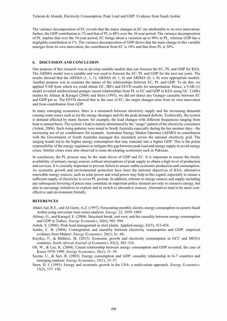
This study also forecasts the total EC, PL and GDP using the VAR model with a 10 year horizon. The forecast results for EC, PL and GDP show positive growth rates at around 1.02%, 1.06% and 1.08%, respectively.

We explore the dynamic relationships among EC, PL and GDP using tools such as GC, IRFs and forecast error variance decompositions with no GC from EC to PL or EC to GDP and also no significant GC from GDP to EC and GDP to PL. Importantly, however, a unidirectional GC is observed from PL to EC and GDP a the 5% level. The estimations confirm that a neutrality hypothesis is valid in the case of EC to PL and GDP and from GDP to EC and PL; however, the feedback hypothesis has been shown for PL to EC and GDP.

Figure 4 shows the impulse response analyses of the three variables, which is carried out to determine the shocks that arise in one variable and whether or not these shocks are transmitted to other variables. The results for the 10-year analysis reveal that one positive standard deviation shock in PL will lead the GDP to rise positively. The result also implies that one standard deviation positive shock to EC will bring about positive changes in GDP. A GDP innovation with a standard deviation of one results in an immediate positive response by about 0.1, indicating that the GDP accelerates by itself.

Figure 4. Impulse response graphs

Table 5. Variance decomposition

Horizon VDA (EC) VDA (PL) VDA (GDP)

EC PL GDP EC PL GDP EC PL GDP

1 1 0.203 0.006 0 0.796 0.011 0 0 0.982

2 0.973 0.286 0.013 0.026 0.614 0.007 0.0004 0.098 0.978

3 0.947 0.336 0.023 0.05 0.477 0.006 0.001 0.186 0.97

4 0.925 0.371 0.034 0.066 0.389 0.006 0.008 0.238 0.958

5 0.90227 0.399 0.048 0.076 0.332 0.007 0.02 0.267 0.944

6 0.88 0.422 0.062 0.083 0.293 0.008 0.036 0.283 0.929

7 0.859 0.442 0.077 0.086 0.265 0.009 0.054 0.291 0.913

8 0.839 0.459 0.091 0.088 0.244 0.011 0.071 0.296 0.896

9 0.822 0.474 0.106 0.089 0.227 0.013 0.088 0.297 0.88

10 0.806 0.487 0.12 0.09 0.214 0.015 0.103 0.298 0.864

Table 5 shows the variance decomposition of the three variables. This test is used to determine the extent of variation, in percentage terms, caused by a variable itself and whether other variables have contributed to it.

207


The variance decomposition of EC reveals that the major changes in EC are attributable to its own innovation; further, the GDP contribution is 1% and that of PL is 48% over the 10-year period. The variance decomposition of PL implies that over the 10-year period, EC brings about a variation up to 90% in PL, whereas GDP has a negligible contribution at 1%. The variance decomposition of GDP shows that the main change in this variable emerges from its own innovation; the contribution from EC is 10% and that from PL is 30%.

6. DISCUSSION AND CONCLUSION

One purpose of this research was to develop suitable models that can forecast the EC, PL and GDP for KSA. The ARIMA model was a suitable and was used to forecast the EC, PL and GDP for the next ten years. The results showed that the ARIMA (1, 1, 1), ARIMA (0, 1, 0) and ARIMA (0, 1, 0) were appropriate models. Another purpose was to examine the nature of the relationships between EC, PL and GDP. To do this, we applied VAR from which we could obtain GC, IRFs and FEVD results for interpretation. Hence, a VAR (1) model revealed unidirectional granger causal relationships from PL to EC and GDP in KSA using GC. Unlike studies by Altinay & Karagol (2004) and Stern (1993), we did not detect any Granger causality between EC and GDP per se. The FEVD showed that in the case of EC, the major changes arise from its own innovation and from contribution from GDP.

In many emerging economies, there is a mismatch between electricity supply and the increasing demands causing some issues such as (a) the energy shortages and (b) the peak demand deficits. Technically, the system is demand affected by many factors: for example, the load changes with different frequencies ranging from hour to annual basis. The system’s load is mainly determined by the “usage” pattern of the electricity consumers (Ashok, 2006). Such rising patterns were noted in South Australia especially during the hot summer days - the increasing use of air conditioners for example. Australian Energy Market Operator (AEMO) in consultation with the Government of South Australia managed this mismatch across the national electricity grid. The surging trends led to the higher energy consumption that may translate into a higher GDP. This is the prime responsibility of the energy regulators to mitigate this gap between peak load and energy supply to avoid energy crises. Similar crises were also observed is some developing economies such as Pakistan.

In conclusion, the PL process may be the main driver of GDP and EC. It is important to ensure the timely availability of primary energy sources without interruptions of peak supply to obtain a high level of production and services. It is crucially important to prevent failure to ensure stable economic production and consumption. As economic growth and environmental protection have been the national objectives of KSA, alternative renewable energy sources, such as solar power and wind power may help in this regard; especially to ensure a sufficient supply of electricity to cover PL periods. In addition, reforms in energy sources and supply including any subsequent lowering of prices may constitute an important policy element not only to conserve energy, but also to encourage initiatives to explore and to switch to alternative sources. Alternatives tend to be more cost-effective and environment friendly.

REFERENCES

Abdel-Aal, R.E., and Al-Garni, A.Z. (1997). Forecasting monthly electric energy consumption in eastern Saudi Arabia using univariate time-series analysis. Energy, 22, 1059–1069.

Altinay, G., and Karagol, E. (2004). Structural break, unit root, and the causality between energy consumption and GDP in Turkey. Energy Economics, 26(6), 985–994.

Ashok, S. (2006). Peak-load management in steel plants. Applied energy, 83(5), 413-424. Jumbe, C. B. (2004). Cointegration and causality between electricity consumption and GDP: empirical

evidence from Malawi. Energy Economics, 26(1), 61–68. Kayıkçı, F., & Bildirici, M. (2015). Economic growth and electricity consumption in GCC and MENA

countries. South African Journal of Economics, 83(2), 303–316. Oh, W., & Lee, K. (2004). Causal relationship between energy consumption and GDP revisited: the case of

Korea 1970–1999. Energy Economics, 26(1), 51–59. Soytas, U., & Sari, R. (2003). Energy consumption and GDP: causality relationship in G-7 countries and

emerging markets. Energy Economics, 25(1), 33–37. Stern, D. I. (1993). Energy and economic growth in the USA: a multivariate approach. Energy Economics,

15(2), 137–150.

208

electricity consumption, peak load and gdp in saudi … · tularam & alsaedi, electricity...

Documents