electricity transmission congestion costs: a review of …€¦ · · 2011-07-28lbnl-54049...

LBNL-54049

Electricity Transmission Congestion Costs: A Review of Recent Reports

Prepared by Bernard C. Lesieutre and Joseph H. Eto Energy Analysis Department Ernest Orlando Lawrence Berkeley National Laboratory University of California Berkeley Berkeley, CA

Environmental Energy Technologies Division October 2003

http://eetd.lbl.gov/ea/EMS/EMS_pubs.html The work described in this report was coordinated by the Consortium for Electric Reliability Technology Solutions and funded by the Office of Electric Transmission and Distribution of the U.S. Department of Energy under Contract No. DE-AC03-76SF00098.

ERNEST ORLANDO LAWRENCE BERKELEY NATIONAL LABORATORY

Disclaimer

This document was prepared as an account of work sponsored by the United States Government. While this document is believed to contain correct information, neither the United States Government nor any agency thereof, nor The Regents of the University of California, nor any of their employees, makes any warranty, express or implied, or assumes any legal responsibility for the accuracy, completeness, or usefulness of any information, apparatus, product, or process disclosed, or represents that its use would not infringe privately owned rights. Reference herein to any specific commercial product, process, or service by its trade name, trademark, manufacturer, or otherwise, does not necessarily constitute or imply its endorsement, recommendation, or favoring by the United States Government or any agency thereof, or The Regents of the University of California. The views and opinions of authors expressed herein do not necessarily state or reflect those of the United States Government or any agency thereof, or The Regents of the University of California. Ernest Orlando Lawrence Berkeley National Laboratory is an equal opportunity employer.

LBNL-54049

Electricity Transmission Congestion Costs: A Review of Recent Reports

Prepared by Bernard C. Lesieutre and Joseph H. Eto Energy Analysis Department

Environmental Energy Technologies Division Ernest Orlando Lawrence Berkeley National Laboratory

University of California Berkeley Berkeley, CA

October 2003 The work described in this report was coordinated by the Consortium for Electric Reliability Technology Solutions and funded by the Office of Electric Transmission and Distribution of the U.S. Department of Energy under Contract No. DE-AC03-76SF00098.

ii

Acknowledgements The authors gratefully acknowledge the reviewers who have provided valuable comments that have improved the clarity and value of this report. These include Eric Allen (NYISO), Mario Depillis and Wayne Coste (ISO-NE), Joe Bowring (PJM), Jing Chen (CAISO), Doug Hale (DOE), Steve Widegren (PNNL), Chris Marnay and Ryan Wiser (LBNL), Thanh Luong and Udi Helman (FERC), Frances Wood (Onlocation), Fernando Alvarado (University of Wisconsin), Shmuel Oren (University of California-Berkeley), Bob Thomas and Tim Mount (Cornell University), and Ed Kahn and Matt Barmack (Analysis Group). Authors accept sole responsibility for all errors/omissions.

iii

Acronyms CAISO California Independent System Operator CRR Congestion revenue right DOE U.S. Department of Energy ECP Energy clearing price FERC Federal Energy Regulatory Commission FTR Fixed transmission right ISO Independent system operator ISO-NE Independent System Operator - New England LMP Locational marginal price MW Megawatt MWh Megawatt hour NOPR Notice of Proposed Rulemaking NYISO New York Independent System Operator PJM Pennsylvania-New Jersey-Maryland Interconnection SMD Standard market design TCC Transmission congestion contract

iv

Table of Contents

Acknowledgments..................................................................................................................... ii Acronyms.................................................................................................................................. iii List of Figures & Tables ........................................................................................................... v Executive Summary .................................................................................................................. vi 1. Introduction ....................................................................................................................... 1 2. Transmission Congestion Costs in a Vertically Integrated Electricity Industry ............... 5 3. Transmission Congestion Cost Calculations in Restructured Electricity Markets............ 9 Uplift Charges ................................................................................................................... 12 System Redispatch Payments ............................................................................................ 13 Congestion Revenues ........................................................................................................ 15 Combining System Redispatch Payments and Congestion Revenues .............................. 17

Summary of Transmission Calculation Cost Methods used in Restructured Electricity Markets ...................................................................................... 18

4. Review of Published Estimates of Transmission Congestion Costs ................................. 21 PJM.................................................................................................................................... 21 ISO-NE ............................................................................................................................. 22 CAISO ............................................................................................................................... 23 NYISO .............................................................................................................................. 24 Federal Energy Regulatory Commission .......................................................................... 25 National Transmission Grid Study (NTGS)...................................................................... 25 A Practical Consideration for the Calculation of System Redispatch Payments .............. 25 Summary of Congestion Cost Review .............................................................................. 27

5. Key Issues for Accurately Determining and Interpreting Congestion Costs .................... 29 Appendix A............................................................................................................................... 37 References................................................................................................................................. 42

v

Figures and Tables

Figure 1. Two Area Network and Corresponding Aggregate Supply Curves. ........................ 5 Figure 2. Production Costs: Constrained and Unconstrained Case ........................................ 7 Figure 3. Dispatch Costs Paid to the Generators ..................................................................... 10 Figure 4. A Constrained Two-Area System and Corresponding Aggregate Supply Curves... 12 Figure 5. Generation Dispatched “out of merit order” ............................................................ 13 Figure 6. Change in Dispatch Payments to the Generators ..................................................... 14 Figure 7. Net Dispatch Cost Change........................................................................................ 15 Figure 8. Dispatch Payments to Generators Separated by the Congested Transmission Line ........................................................................................................................................... 16 Figure 9. Revenues Collected from the Loads......................................................................... 16 Figure 10. Congestion Charges................................................................................................. 17 Figure 11. Different Approaches to the Calculation of “Congestion Costs”............................ 20 Figure 12. A Two-Area System in which Transmission Expansion to Eliminate Congestion will Increase Total Costs. ...................................................................................... 31 Figure 13. Dispatch Payments to Generators............................................................................ 32 Figure 14. Constrained “out of merit order” Dispatch and Uplift Costs .................................. 33 Figure 15. Net Change in Sum of Consumer and Producer Surplus between Constrained and Unconstrained cases. .......................................................................................................... 35 Figure A1. A Plot of Consumer Surplus and Producer Surplus, and Congestion Charges For Constrained Case................................................................................................................ 37 Figure A2. A Plot of Consumer Surplus and Producer Surplus for Unconstrained Case......... 38 Figure A3. A Change in Consumer Surplus, Producer Surplus and Congestion Charges when the Transmission Capacity Limit is Increased to Allow Uncongested Operation .......... 39 Figure A4. Transfers and Changes in Consumer & Product Surplus ....................................... 40

Table 1. Summary of Congestion Costs Reported by ISOs, DOE and FERC......................... 2 Table 2. Dispatch, Dispatch Costs, and Revenues for the Unconstrained and Constrained System....................................................................................................................................... 17 Table 3. Comparison of Congestion Costs Associated with System Redispatch Payments, Congestion Revenues and Total Costs...................................................................................... 18 Table 4. Calculations Used to Determine Congestion Costs in Restructured U.S. Electricity Markets.................................................................................................................... 19 Table 5. Summary of Congestion Costs Reported by ISOs, DOE, and FERC........................ 27

vi

Executive Summary Recently, independent system operators (ISOs) and others have published reports on the costs of transmission congestion. The magnitude of congestion costs cited in these reports has contributed to the national discussion on the current state of theU.S. electricity transmission system and whether it provides an adequate platform for competition in wholesale electricity markets. This study reviews reports of congestion costs and begins to assess their implications for the current national discussion on the importance of the U.S. electricity transmission system for enabling competitive wholesale electricity markets. As a guiding principle, we posit that a more robust electricity system could reduce congestion costs; and thereby, 1) facilitate more vibrant and fair competition in wholesale electricity markets, and 2) enable consumers to seek out the lowest prices for electricity. Yet, examining the details suggests that, sometimes, there will be trade-offs between these goals. Therefore, it is essential to understand who pays, how much, and how do they benefit in evaluating options (both transmission and non-transmission alternatives) to address transmission congestion.1 To describe the differences among published estimates of congestion costs, we develop and motivate three ways by which transmission congestion costs are calculated in restructured markets. The assessment demonstrates that published transmission congestion costs are not directly comparable because they have been developed to serve different purposes. More importantly, critical information needed to make them more comparable, for example in order to evaluate the impacts of options to relieve congestion, is sometimes not available. Congestion costs arise when, in order to respect transmission constraints, some higher-cost generation is dispatched in favor of lower-cost generation that would otherwise be used (in the absence of the constraint). The additional payments to higher-priced generation (above that dispatched in least-cost order) may be shared equally among customers as an Uplift Charge. Alternatively, when locational marginal pricing (LMP) is used, System Redispatch Payments2 reflect the difference in payments to generators from an ideal uncongested system. Under LMP, customers that import energy incur additional congestion charges in proportion to the difference between energy prices at the generation source and the load. The sum of these congestion charges is called Congestion Revenues. Corresponding Congestion Revenue Rights determine the allocation of Congestion Revenues. Uplift charges and system redispatch payments both measure changes in generation payments due to congestion under different market

1 It is also important to recognize that the capacity of the transmission system is limited. Operators observe many constraints in order to ensure reliability. Relieving any one constraint will only increase capacity up to the point at which the next constraint becomes binding. In some cases, there may be no good (i.e., lower cost) alternatives to existing levels of congestion. 2 We refer to change in payments to generators from the market perspective as “System Redispatch Payments” to distinguish these payments from the change in production costs, which are often labeled “Redispatch Costs.”

vii

institutions. Congestion revenues reflect transportation costs equal to the difference between what customers pay and generators receive for transported energy. Table EX-1 lists the recent studies published by ISOs, the congestion costs reported in each, and the types of calculation methods used Table EX-1. Summary of Congestion Costs Reported by ISOs, DOE, and FERC Period Congestion Costs

($Million) Congestion Cost-Calculation Method(s)

PJM [1] 1999 53 PJM [1] 2000 132 PJM [1] 2001 271 PJM [2] 2002 430

Congestion Revenues

ISO-NE [3] 5/99-4/00 99 ISO-NE [3] 5/00-4/01 120

Uplift Charges3

ISO-NE [4] 2003 50 – 300 System Redispatch Payments CAISO [5] 2000 391 CAISO [5] 2001 107 CAISO [6] 2002 42

Congestion Revenues

CAISO [7,8] 2005 -7.47 – 306 System Redispatch Payments + Congestion Revenues

NYISO [9] 2000 1,240 NYISO [9] 2001 570

System Redispatch Payments (est) + Congestion Revenues

NYISO [10] 2000 517 NYISO [10] 2001 310 NYISO [11] 2002 525

Congestion Revenues

FERC [12] 6/00-8/00 891 System Redispatch Payments (partial) + Congestion Revenues

DOE [13] 157 – 457 System Redispatch Payments + Congestion Revenues

[1] PJM Interconnection, State of the Market Report 2001 (PJM 2002) [2] PJM Interconnection, State of the Market Report 2002 (PJM 2003) [3] ISO New England (ISO-NE), Annual Markets Report (ISO New England 2002a) [4] ISO New England, RTEP02 (ISO New England 2002b) [5] California Independent System Operator (CAISO) Market Analysis Reports (CAISO 2000, 2001a) [6] CAISO, 2002 Annual Report on Market Issues and Performance (CAISO 2002) [7] CAISO, Path 15 Expansion Economic Benefit Study: Phase II (CAISO 2001c) [8] CAISO, Potential Economic Benefits to California from Expanding Path 15 (CAISO 2001d) [9] New York Congestion and Physical Constraint Cost Estimates (POWERGEM 2002) [10] 2001Annual Report on the New York Electricity Markets (Patton and Wander 2002) [11] 2002 State of the Market Report: New York Electricity Markets (Patton 2003) [12] Federal Energy Regulatory Commission (FERC), Electric Transmission Constraint Study (FERC 2002) [13] U.S. Department of Energy (DOE), National Transmission Grid Study (DOE 2001) We draw the following conclusions from our analysis of published costs of transmission congestion:

3 ISO New England’s congestion cost calculation method was modified in March 2003.

viii

1. Information about the operation of congestion revenue rights markets is needed to assess the impacts of congestion revenue charges on consumers.

Some of the congestion revenue charges incurred by consumers may be offset by congestion revenue rights that return these charges to them. The process of distributing the revenue from congestion on a transmission path is different for different ISOs; information about the process used by a given ISO is necessary to assess the final impact of congestion revenue charges on costs to consumers in that ISO’s territory.

2. Information on generators’ offers is needed to assess system redispatch payments. ISOs’ reports of congestion costs, which typically refer only to congestion revenue costs handled by each ISO’s market settlement process, do not permit direct evaluation of system redispatch payments that might be influenced by relief of transmission congestion. In addition, generator offer curves are needed to estimate system redispatch payments. This information is generally not available, yet it is needed in order to assess the impacts of options to relieve congestion.

3. Many studies presume that generator offers reflect competitive market conditions.

While information on generator offer curves would enable one to estimate system redispatch payments, using offer curves alone may understate the full value of relieving congestion if the market is not competitive (i.e., if generators can unfairly raise their offers above their marginal cost of production). Relieving congestion will reduce generators’ opportunities to exercise market power; it is appropriate to include consideration of this effect when assessing the benefits of options to relieve congestion.

4. Customer costs may rise as a result of reducing congestion. Generally speaking, reducing congestion will likely increase electricity prices in exporting regions, which in turn is expected to be offset by lower prices in the importing regions. Yet, whether total average consumer costs increase or decrease with transmission capacity expansion, which reduces congestion, depends on price changes and levels of demand in each region. For example, in planning studies of decreased congestion conducted for California, an overall increase in consumer costs is observed in many scenarios.

5. Minimizing consumer costs may not increase aggregate social wealth.

Economic theory suggests that policy decisions should consider the effect of transmission congestion relief on the sum of consumer surplus and producer surplus. Yet, as noted in the previous finding, relieving congestion would, in some instances, increase, not lower, consumer costs. Thus, although economic theory suggests that maximizing aggregate wealth is an appropriate policy objective for congestion relief

ix

efforts, it also is appropriate to consider tempering this objective with that of lowering consumer costs.4

6. There is no standardized conceptual framework for studies of congestion costs.

Our survey of ISO and government reports on congestion costs, summarized in Table EX-1, reflects a diversity of practices, which makes it difficult to compare reported congestion costs across institutions. This is hardly surprising, as there are several perspectives from which the economic and financial impacts of congestion can be viewed. In the future, it would be useful if ISO reports clearly stated the different purposes to which the various measures apply and then apply the measurement concepts in more standardized fashion.

4 Economic theory offers an option to reconcile these differences: maximize producer and consumer surplus and devise a system of lump-sum transfers to achieve some equitable design.

1

1. Introduction Transmission congestion occurs when there is not enough transmission capability to support all requests for transmission services, and in order to ensure reliability, transmission system operators must re-dispatch generation or, in the limit, deny some of these requests to prevent transmission lines from becoming overloaded. In other words, transmission congestion does not refer to deliveries that are simply held up or delayed (as in traffic congestion); it refers to requests for deliveries (transactions) that cannot be physically implemented as requested. The cost of transmission congestion, assuming that demand is fixed and must be met, is the net cost of the replacement power that must be supplied by other means (e.g., from generators located closer to the loads to be served) to make up for deliveries that cannot be executed as requested. Recent published reports by independent system operators (ISOs) and others (listed in Table 1) present widely varying estimates of congestion costs. The objective of our report is to determine how these costs were calculated and how they can be accurately interpreted and used. Understanding these reported costs is crucial if they are to be used in making decisions about whether and how to address transmission congestion – e.g., by expanding/reinforcing the transmission system to increase its capability to deliver electricity or pursuing non-transmission strategies that accomplish the same end, such as increasing generation capacity closer to the load it serves or engaging in demand-side management. The cost of transmission congestion establishes an upper limit on the value of alleviating congestion.5 If the value of alleviating congestion exceeds the cost of a particular strategy to do so, then that strategy will lower total cost of service. It is equally important to recognize that the capacity of the transmission system is limited. Operators observe many constraints in order to ensure reliability. Relieving any one constraint will only increase capacity up to the point at which the next constraint becomes binding. In some cases, there may be no good (i.e., lower cost) alternatives to existing levels of congestion. Table 1 summarizes recent reported congestion costs. We demonstrate that significant differences among the methods and data used to calculate these costs make it difficult to compare the estimates. Understanding how congestion costs have been derived and thus what they can and cannot tell us is a key first step in being able to assess whether and how to relieve congestion. We also identify additional information needed to permit comparison among the different reports of congestion costs. The establishment of competitive wholesale electricity markets rests on the guiding principle that competition will facilitate more vibrant and fair competition in wholesale electricity trade, and enable consumers to seek out the lowest electricity prices. It seems

5 An option may only partially relieve congestion; generally speaking, relieving any particular constraint is effective only up to the point at which the next constraint becomes binding. At the same time, relieving transmission congestion may be only one of several values offered by a generation, transmission, or demand-side option under consideration; for example, enhancing system reliability would be another value relevant to a comprehensive evaluation.

2

logical that reducing congestion costs would contribute to this objective; however, simultaneously satisfying these goals may not always be possible. Among our findings is that reducing congestion may cause prices to rise for some customers or loads (we use the terms “load” and “customer” or “consumer” interchangeably in this report). Who pays for energy and congestion, and how much they pay, are questions that must be addressed in evaluating options to increase competition in wholesale electricity markets by reducing transmission congestion. Table 1. Summary of Congestion Costs Reported by ISOs, DOE, and FERC Period Congestion

Costs ( $ Million)

Source

PJM 1999 53 PJM 2000 132 PJM 2001 271 PJM 2002 430

PJM Interconnection State of the Market Reports (PJM 2002, 2003)

ISO-NE 5/99-4/00 99 ISO-NE 5/00-4/01 120

ISO New England (ISO-NE) Annual Markets Report (ISO NE 2002a)

ISO-NE 2003 50 – 300 ISO-NE, RTEP02 (ISO NE 2002) CAISO 2000 391 CAISO 2001 107 CAISO 2002 42

CAISO Market Analysis Reports (CAISO 2000, 2001a, 2003)

CAISO 2005 -7.47 – 306 CAISO, Studies of benefits of expansion of Path 15 (CAISO 2001c, 2001d)

NYISO 2000 1,240 NYISO 2001 570

New York Congestion and Physical Constraint Cost Estimates (POWERGEM 2002)

NYISO 2000 517 NYISO 2001 310 NYISO 2002 525

Annual Reports on the New York Electricity Markets (Patton and Wander 2002, Patton 2003)

FERC 6/00-8/00 891 Electric Transmission Constraint Study [FERC (Federal Energy Regulatory Commission) 2001]

DOE 157 – 457 National Transmission Grid Study [DOE (U.S. Department of Energy) 2002]

Following the introduction, this report is organized as follows: In Section 2, we introduce a stylized example of the “cost” of transmission congestion in a vertically integrated utility industry. This example allows us to illustrate the key operational concept associated with transmission congestion: the redispatch of generation to respect a transmission constraint. We also describe the role of transmission congestion costs in measuring the value of strategies to reduce congestion. Section 3 illustrates the computation of transmission congestion costs in restructured electricity markets. We introduce two elements of restructured markets that increase the complexity of these calculations – first, uniform market clearing prices and, second, locational marginal prices (LMPs) – both of which are derived from generators’ offers to sell electricity. We also describe and motivate the use of three generic approaches to calculating transmission congestion costs in restructured markets; these generic calculation approaches underlie all recent published estimates of congestion costs.

3

In Section 4, we review published estimates of transmission congestion costs and link each estimate to one or more of the three cost-calculation methods identified in Section 3. Our objective is to demonstrate that these methods are different by design, often because the congestion cost estimates that they support are used for different purposes; therefore, the estimates are not comparable. In Section 5, we discuss methodological challenges that must be overcome to develop more consistent estimates of congestion costs than are currently available. This discussion clarifies that currently available, published information is insufficient to make these comparisons consistently and describes the difficulty of relying only on published estimates to determine the value of activities to reduce congestion.

5

2. Transmission Congestion Costs in a Vertically Integrated Electricity Industry Transmission congestion is not a unique feature of restructured electricity markets. Transmission system operators always have had to limit power flows (and will continue to have to do so) to maintain safe operating (or reliability) margins on the electricity grid.6 To illustrate the relationship between the production cost impacts of transmission congestion and the evaluation of options to reduce these costs, we first review how the “costs” of transmission congestion arise in the vertically integrated industry structure that prevailed for much of the industry’s history in the U.S. To illustrate the methods and to discuss the issues that will appear throughout this document, we rely on an elementary and stylized example shown in Figure 1. To focus on congestion issues, we neglect other transmission line usage tariffs, generator limits, and subtle price differences that result from nominal losses in the system. We do, however, consider hard transmission capacity constraints that may arise from thermal, voltage, and stability considerations.

(a)

(b) Figure 1. A two-area network (a) and corresponding aggregate supply curves for the generation in each area (b). Uncongested conditions are shown in this

6 The nature of electricity and the interconnectedness of the networks over which it flows means that it is extremely important to maintain safe operating margins through the coordinated efforts of all interconnected transmission system operators. Failure to operate the entire network a coordinated manner increases the likelihood that loss of one or more elements (e.g., a generator or transmission line) could lead to a catastrophic, cascading blackout of the entire network.

Area A 0 100 200 300 400 500 600 700 800 900 1000 1000 900 800 700 600 500 400 300 200 100 0 Area B Supply

20

22

24

26

28

30

32

$/MWh

20

22

24

26

28

30

32

$/MWh Area A Load Area B Load

Area A

Area B

A B

200 MW

500 MW load

500 MW load

700 MW supply

300 MW supply

6

diagram. Without congestion, the intersection of the curves determines the dispatch, 700 megawatts (MW) from Area A generators and 300 MW from Area B generators. For the two-area system shown in Figure 1 (a), each of the areas serves a totally inelastic load of 500 megawatts (MW). A transmission line that connects the areas allows energy transfer between them. In Figure 1 (b) we show the aggregate supply curves for the generators in each area; each curve plots the marginal cost of generation vs. supply. The blocks of energy available to meet load are ordered from lowest price to highest price to obtain the supply curve. At any point along this curve, the marginal cost is the cost necessary to physically generate the next unit of energy for any given amount of supply. Looking from left to right on the plot in Figure 1 (b), we can follow the generation marginal cost vs. supply for generators in Area A. Looking from right to left, we follow the generation marginal cost vs. supply for generators in Area B.7 The supply curves are presented in this fashion to illustrate the constraint that the total supply equals the total (inelastic) demand of 1,000 MW. The reader is reminded that there is 500 MW of demand in each area by labels over the top of the plot. With no capacity limit on transmission between areas, we observe that the unconstrained, least-cost dispatch will be 700 MW for generators in Area A and 300 MW for generators in Area B. The generators in Area A serve their native load of 500 MW and export 200 MW of power to Area B. In Figure 2, a transmission constrained system illustrates how production costs are increased due to the constraint, and how production costs would change if the constraint were relieved (i.e., if the system returned to its original, unconstrained state, as described in Figure 1). In this system, transfers between Areas A and B are limited to 100 MW. To respect this constraint, load in Area B must rely on more expensive generation in its own area rather than lower-cost generation that could be dispatched from Area A if there were no constraint. In this example, total production costs exceed those of the earlier example in which there was no limit on the amount of power that could be transferred from Area A to Area B. The difference in production costs between the constrained and unconstrained examples is a measure of the cost of congestion under a vertically integrated utility industry structure. In a vertically integrated industry, the same firm owns and operates all generation, transmission, and distribution. The cost of maintaining adequate safety margins, reflected by the 100-MW transmission constraint in Figure 2, is simply “rolled in” as one element of the cost of providing reliable electric service to the entire franchise of retail customers (in this case, all customers in Areas A and B). The shaded area under the two curves represents the total production cost of energy to supply these loads.

7 It is useful to observe that, viewed from the perspectives of generators in Area A, the supply curve of generation in Area B looks like and in fact acts as a “demand curve” on generation supplied from Area A. This presentation of a reverse supply curve to investigate the value of transmission appears in several places in the literature including (Hunt 2002), (Joskow and Tirole 2003), and (Barmack et al 2003).

7

(a)

(b)

(c) Figure 2. The shaded regions represent production costs for (b) the constrained case and (c) the unconstrained case. Note that production costs are lower in the unconstrained case. Figure 2 also illustrates the decrease in production costs (i.e., the production cost savings) that would result from increasing the transfer limit between Areas A and B from 100 MW to 200 MW. Given appropriate regulatory or other incentives (e.g., mandates from governing bodies), vertically integrated firms assess strategies that could lower the total


20

22

24

26

28

30

32

$/MWh

20

22

24

26

28

30

32


100 MW Transmission Constraint

Area A Production Costs

Area B ProductionCosts


20

22

24

26

28

30

32

$/MWh

20

22

24

26

28

30

32


Area A Production Costs

Area B ProductionCosts

Decrease in production costs achieved through transmission expansion

A B

100 MW

500 MW load

500 MW load

600 MW supply

400 MW supply

8

cost of providing electricity service (these strategies include building new generation closer to the load served, building new transmission lines to access lower-cost generation in locations that are remote from the load served, or undertaking demand-side programs to reduce loads). The decrease in production costs illustrated in Figure 2 would be a measure of the value of one or more of these strategies from the standpoint of reducing congestion. The area representing the decrease in production costs also represents, in this case, the increase in consumer surplus between the congested and uncongested scenarios. From the perspective of Area A generators, the supply curve of generation for Area B looks and acts like a demand curve for generation supplied by Area A. The consumers in Area B are evidently willing to pay at least the price represented by the demand curve; and consumers benefit from the lower-priced power made available through transmission capacity enhancement (once rates are adjusted to reflect lower costs). The measure of this benefit is the change in consumer surplus. Because this graph shows only production costs, there is no producer surplus. Although this discussion is couched in the language of a vertically integrated firm, it also has a bearing on transmission planning in restructured electricity markets. We will return to this topic in Section 5 when we discuss policy decisions to increase social wealth through the increase in the sum of consumer and producer surplus.

9

3. Transmission Congestion Cost Calculations in Restructured Electricity Markets In a restructured electricity market generators are owned by many different firms, the transmission system is operated (is not owned) by a separate business entity, and distribution is provided to many, distinct franchises of customers. In this market, the “cost” of maintaining safe transmission operating margins can be defined in a variety of ways. Each definition reflects the design objectives and cost-recovery policies of the particular market. A critical element is specifying how the costs of safe operating margins are recovered from or paid to customers receiving electricity service and/or are paid to or recovered from the generators. Although these costs are defined differently in different markets, they are usually referred to using the same term: “transmission congestion costs.” We identify three generic approaches that have been used individually and in combination to determine reported costs of congestion in restructured electricity markets. To understand these generic approaches, it is first necessary to understand two core elements of restructured electricity markets: (a) uniform market clearing prices and (b) locational marginal prices (LMPs), both of which are derived from generators’ offers to sell electricity. The discussion that follows is based on the understanding that the principal objective of electricity industry restructuring is to rely on competition among power suppliers to lower costs to consumers. (It is not our intent to defend this position or review other aspects of competitive markets.) This basic principle implies that higher energy prices are an incentive for the introduction of new, lower-cost sources of supply. Transmission can be used to enlarge the sources of supply available to meet demand for electricity. Transmission congestion in this context is the consequence of a physical limit on the transmission system’s capability to accommodate all requests to using lower-cost, remotely located generation rather than more expensive local generation to meet demand. All restructured U.S. electricity markets rely on offer-based, centralized, wholesale trade in which generators offer to sell blocks of electricity at fixed prices. Market makers (currently ISOs) clear the market by arranging the offered quantities from least to most expensive and accepting all offers necessary to meet demand. This process is similar to the task performed by the dispatcher in the vertically integrated industry structure; however, in a restructured industry the prices offered for individual blocks of generation are set by the generators. In the examples below, the supply curve of offers will replace the supply curve of generator production costs shown in the previous section for the vertically integrated industry. If the market is competitive, the supply curve created by aggregating generator offers should closely approximate the system marginal production cost of generation. The market clearing price is set based on the last accepted offer and is “uniform”; that is, each accepted offerer is paid the same price regardless of the original offer made. The

10

market clearing price for a given region is the LMP of electricity for that region.8 In other words, the market clearing price is, to a first approximation, the cost of producing one more (or one less) megawatt hour (MWh) of electricity in that region. This fact can be observed by reviewing the supply curve of generators’ offers where we can see that the market clearing price is the marginal cost of supplying (or more accurately, marginal willingness to supply, if offers differ from costs) one additional (or one less) MWh of electricity beyond the amount used to set the market clearing price. Figure 3 illustrates the application of these principles to a restructured market without congestion. This example uses the same physical circumstances presented in Figure 1, which illustrated least-cost dispatch for an uncongested, vertically integrated market with two areas, A and B. The generators in Area A serve their native load of 500 MW and transport 200 MW of power to Area B. The LMP for all generators is $25/MWh. Under this unconstrained operating condition, the total dispatch costs paid to the generators are equal to:

(700 MW)($25 /MWh) +(300 MW)($25 /MWh) = $25,000 /h.

These funds come directly from the loads:

(500 MW)($25 /MWh) + (500 MW)($25 /MWh) = $25,000 /h

where consumers in both areas pay an energy price equal to $25 /MWh.

Figure 3. The shaded regions show the dispatch costs paid to the generators in each area from a uniform clearing price market without congestion. Assuming the loads are charged the same price, the same shaded area indicates the revenue collected from the loads.

8 This discussion suppresses important technical details regarding differences between zonal and nodal pricing. Locational marginal prices, for the purposes of this report, refer only to the broad principle of prices that vary according to location within the grid.


20

22

24

26

28

30

32

$/MWh

20

22

24

26

28

30

32


Paid to “A” gens. Paid to

“B” gens.

11

The reader will note that in this case the costs paid by loads and the revenues received by suppliers appear to increase relative to costs in the production-cost model in the previous section of this report. In the face of this increase, it is reasonable to ask why it makes sense to use a uniform price auction rather than a “pay-as-bid” auction in which suppliers would be paid according to their actual offers. The answer is that the offer curves would be different in a pay-as-bid auction; suppliers would not have an incentive to offer marginal costs but would offer all their capacity at the expected market clearing price. Despite this difference, economic theory (the revenue equivalence theorem) suggests that the two approaches will nonetheless yield similar results (Thomas et al. 2000). The reader will also note the significant supplier surplus available under the uniform price approach, which indicates that the revenues received by suppliers exceed production costs. In a competitive environment, this surplus is an incentive for the introduction of new, lower-cost generation that may, in the long term, decrease total costs to customers. Moreover, using the uniform price approach is consonant with the practice of today’s restructured U.S. electricity markets, which have all adopted the uniform price auction. Figure 4 (a) shows a congested system in which the line connecting the Areas A and B is at its capacity limit of 100 MW. Because of this transmission constraint, Area A generators produce a total of only 600 MW: 500 MW serve the load in Area A, and 100 MW exported to Area B. With the decrease in generation in Area A compared to the uncongested case, the marginal cost of generation offers for Area A (i.e., the LMP for Area A) has decreased slightly to $23 /MWh. That is, the marginal cost to physically supply the next unit of energy from Area A generators is equal to $23 /MWh. In Area B, where the generation has increased over the uncongested case to 400 MW, the marginal cost of generation offers (i.e., the LMP for Area B) has increased to $30 /MWh. This is observed on the supply curves shown in Figure 4 (b). The examples of transmission congestion described above enable us to examine methods for collecting payments from loads and making payments to generators. How much the generators are paid and what revenues are collected from the loads depend on the market design and policies of the transmission system operator. We have identified three generic approaches that are used to address congestion costs in restructured U.S. electricity markets: 1. Uplift Charges 2. System Redispatch Payments 3. Congestion Revenues These three methods are explained in the following subsections in relation to the example two-area system shown in Figure 4 and described above.

12

(a)

(b) Figure 4. A constrained two-area system (a) and corresponding aggregate supply curves (b). The 100-MW transmission capacity constraint limits Area A generation to 600 MW. This necessitates a corresponding increase in generation in Area B over the unconstrained condition. Uplift Charges Uplift Charges suppress the differences in LMPs between the two areas in our example system and instead rely on a single uniform price for energy throughout the system. This method is closest in spirit to the situation in a vertically integrated industry, because it equates congestion costs with the change in dispatch payments associated with taking additional generation on the congested side of an interface “out of merit order”9, which is sometimes called the cost of “redispatch.” In the Uplift Charge approach, the system operator declares a uniform market clearing price, which we assume is equal to the price in the unconstrained system in our example. Any generator dispatched “out of merit order” because of congestion is paid its actual offer price, but these payments do not influence the market clearing price. In our example, the dispatch costs paid to the generators are represented by the total shaded areas in Figure 5 and are approximately equal to: (600 MW)( $25 /MWh) +(300 MW)($25 /MWh) + (100 MW)( $27.50 /MWh)

= $25,250 /h.

9 The term “out of merit order” has its origin in the unit commitment problem, in which decisions are made about which units to operate. Those chosen for reasons other than least cost (e.g., reliability, congestion) are said to be dispatched out of merit order.


20

22

24

26

28

30

32

$/MWh

20

22

24

26

28

30

32


100 MW Transmission Constraint

A B

23 $/MWh 30 $/MWh

100 MW

500 MW load

500 MW load

600 MW supply

400 MW supply

13

The uplift costs resulting from congestion in this case are equal to $250 /h. The source of these funds is ultimately the loads (consumers), which share the costs equally in this market design. The combined energy and uplift costs (price) to the loads is: ($25,250 /h) / (1,000 MW) = $25.25 /MWh, or just slightly higher than the uncongested price of $25 /MWh. With the declared market clearing price equal to the uncongested price, the apparent “congestion cost” under the uplift approach is the difference in generation offers over and above the market clearing prices of the unconstrained system (Figure 2 (c)) and the constrained system (Figure 2 (b)). Figure 5. The shaded area represents the dispatch costs paid to the generators in both areas. Note that 100 MW of power come from generators in Area B dispatched “out of merit order” (their higher-cost supply would not be used in the unconstrained case). One of the drawbacks of the uplift approach is that it does not, by itself, provide a strong economic incentive to site new generation where it is most needed. This lack of incentive may inhibit the long-term benefits of competition among suppliers because new generation will not necessarily be developed in areas where it could drive prices down. System Redispatch Payments The Uplift Charge approach suppresses differences in LMP between two areas separated by a transmission constraint. Acknowledging the differences in LMP between areas is the basis of the System Redispatch Payments approach to determining congestion costs. This approach is also related to measurement of transmission congestion costs in a vertically integrated industry in that it focuses on the question: how does the total cost of system dispatch change because of the congested interface between two regions? However, in restructured markets, the uniform market clearing price, set at the distinct LMP for each region, is substituted for the supply curve of generation costs that would be used in the vertically integrated structure. The cost of system redispatch is determined by


20

22

24

26

28

30

32

$/MWh

20

22

24

26

28

30

32


Generation dispatched “out of merit order”

Uplift Costs ≈ 250 $/h

14

comparing total dispatch payments to suppliers in the two regions to the total dispatch payments assuming no constraint. The change in revenue paid to generators for dispatch away from the uncongested case is easily calculated:

(600 MW) ($23 /MWh) +(400 MW)($30 /MWh) - (700 MW)($25 /MWh) – (300 MW)($25 /MWh) = $800 /h.

This quantity is represented graphically by the difference in areas shown in Figure 6 and by the darker shaded area in Figure 7.

Figure 6. The difference between the shaded areas represents the change in dispatch payments to the generators relative to payments in the uncongested case. In Area B, the price increased relative to the uncongested price; in Area A, the price decreased. The change in dispatch payments to generators because of congestion may be positive, as in our example, or negative.


20

22

24

26

28

30

32

$/MWh

20

22

24

26

28

30

32


Dispatch cost decrease

Dispatch cost increase

15

Figure 7. The change in dispatch payments to generators is the darker shaded area on the right edge of the plot. This area is obtained by mapping the area corresponding to the reduced dispatch costs in Area A into the area corresponding to the increased generation costs in Area B. The remaining area on the right represents the net generation dispatch payment increase for this example. Congestion Revenues The third approach to calculating congestion costs, the Congestion Revenues method, is based on the policy common among ISOs of paying generators a region-specific LMP for their output regardless of the region where the generation is used to serve load, and, at the same time, charging all loads within a given region a single, region-specific LMP. The difference between what is collected from loads and what is paid out to generators is used to compensate the holders of the rights to transfer power from one region to the other.10 In the constrained example, the LMP in Area A is $23 /MWh and the LMP is Area B is $30 /MWh. The dispatch payments to generators using LMPs and a uniform price auction are represented by the shaded areas in Figure 8 and are equal to: (600 MW) ($23 /MWh) + (400 MW) ($30 /MWh) = $25,800 /h. Using LMPs, the money paid by the loads exceeds that paid to the generators. The revenues collected from the loads are represented graphically by the shaded areas in Figure 9 and are equal to:

(500 MW)($23 /MWh) +(500 MW)($30 /MWh) = $26,500 /h.

10 These rights are called Congestion Revenue Rights (CRRs) in the FERC Standard Market Design (SMD) Notice of Proposed Rulemaking (NOPR). They are called Financial Transmission Rights (FTRs) in the more recent FERC Whitepaper on Wholesale Power Market Platform.


20

22

24

26

28

30

32

$/MWh

20

22

24

26

28

30

32


Equal areas

Net dispatch cost change

16

Figure 8. The shaded area represents the dispatch payments to the generators in the two areas that are separated by the congested transmission line. The LMP corresponding to 600 MW from Area A is $23 /MWh. The LMP corresponding to 400 MW from Area B is $30 /MWh. Figure 9. The shaded areas represent the revenues collected from the loads. Note that the amount paid by all 500 MW of load in Area B is the Area B LMP of $30 /MWh. The difference between what the loads pay and what the generators receive results entirely from congestion. Thus, it is natural for the ISO to refer to this difference as “congestion costs.” This difference also equals the sum of congestion charges along each of the constrained transmission lines. The congestion charge is the product of the power flow and the LMP differences along the line and is represented graphically by the shaded area in Figure 10. A quick check confirms that the difference between load revenues and dispatch payments:

$26,500 /h – $25,800 /h = $700 /h is equal to congestion charges:


20

22

24

26

28

30

32

$/MWh

20

22

24

26

28

30

32



20

22

24

26

28

30

32

$/MWh

20

22

24

26

28

30

32


Paid to “A’ gens.

Paid to “B” gens.

Paid by “A” loads

Paid by “B” loads

17

(100 MW)($30-23 /MWh) = $700 /h. Figure 10. The shaded area represents the congestion charges. In this case, 100 MW of power is transferred from Area A where the generators are paid $23 /MWh to Area B where the loads pay $30 /MWh for the same energy. The congestion charges are the excess payments received from the loads over the dispatch payments to the generators.

The congestion charges of $700 /h, paid by the loads, are distributed according to the market settlement policy. Each ISO has a policy for the disbursement of these funds. Typically, they are allocated to owners of the Congestion Revenue Rights (CRRs) for the congested transmission path between areas. Table 2 summarizes the system conditions for the uncongested and congested cases described above. The data include MWs of generation dispatched, dispatch payments to generators, and revenues received from loads. In the constrained case, we can observe increased dispatch costs as well as revenues from loads that exceed dispatch costs.

Combining System Redispatch Payments and Congestion Revenues The congestion costs paid by loads will necessarily include changes in generator dispatch payments because loads are charged for energy they use. These congestion costs will also include the net congestion revenues resulting from the difference between the prices paid to generators and the prices charged to loads. The net congestion revenues that must be recovered, however, depend both on the total congestion revenues and the amount and

Table 2. Dispatch, dispatch costs, and revenues for the unconstrained and constrained systems. Unconstrained System Constrained System MWs

Dispatched Dispatch costs paid to generators

Revenues received from loads

MWs Dispatched

Dispatch cost paid to generators

Revenues received from loads

Area A 700 MW $17,500 /h $12,500 /h 600 MW $13,800 /h $11,500 /h Area B 300 MW $7,500 /h $12,500 /h 400 MW $12,000 /h $15,000 /h Total 1,000 MW $25,000 /h $25,000 /h 1,000 MW $25,800 /h $26,500 /h


20

22

24

26

28

30

32

$/MWh

20

22

24

26

28

30

32


Congestioncharges

18

allocation of congestion revenue rights.11 Thus, there are two elements of congestion costs: 1. System redispatch payments resulting from congestion (see Figure 7), and 2. Total congestion revenues (see Figure 10). A third element may be inferred if information is available about CRRs: 3. Total costs to loads resulting from congestion, which equals the sum of system redispatch payments and congestion revenues, less any funds returned to the loads through an allocation of CRRs or other means. These elements correspond to methods of calculating congestion costs, which in turn correspond to different congestion costs that could be reported for our two-area example above, as shown in Table 3.

Table 3. Comparison of Congestion Costs associated with System Redispatch Payments, Congestion Revenues, and Total Costs to Loads.

“Congestion Costs” for Previous Example

System Redispatch Payments $800 /h Congestion Revenues $700 /h

Total costs to loads (without CRRs) compared to an uncongested case (Method 1 + Method 2)

$1,500 /h

Summary of Transmission Calculation Cost Methods used in Restructured Electricity Markets We have illustrated that three general methods of calculating congestion costs are used in restructured U.S. electricity markets. These methods are outlined in Table 4 and summarized graphically in Figure 11.

11 There is ongoing debate in the industry regarding the adequacy of various methods for redistributing congestion charges collected by ISOs. In an omniscient allocation of congestion revenue rights, all revenues might be returned. Empirical analysis of CRRs has shown that actual performance is mixed (Siddiqui et al. 2003).

19

Table 4. Calculations Used to Determine Congestion Costs in Restructured U.S. Electricity Markets

Uplift Charges

Congestion costs = dispatch payments out of merit order

Congestion costs are equal to the increased dispatch payments by the market to generators out of merit order. The dispatch payments are calculated using a uniform market clearing price for most generation. However, generators dispatched out of merit order because of congestion are paid at their offer prices. The uplift charge is shared equally among the consumers.

System Redispatch Payments

Congestion costs = change in dispatch costs

Congestion costs are equal to the difference in dispatch payments by the market to generators in the congested case relative to costs for the uncongested case. The dispatch payments are calculated using LMPs.

Congestion Revenues

Congestion costs = congestion charges

In a market that uses LMPs, congestion revenues are the valuation of transmission of energy across a congested interface. Neglecting losses, these revenues equal the product of the energy flow and the price. Congestion revenues are also equal to the difference between what consumers pay for energy and what generators are paid for supply

20

(Uplift Costs)

(System Redispatch Cost)

(Congestion Revenues)

Figure 11. Different approaches to the calculation of “congestion costs”


20

22

24

26

28

30

32

$/MWh

20

22

24

26

28

30

32


Generation dispatched “out of merit order”

Congestion uplift costs


20

22

24

26

28

30

32

$/MWh

20

22

24

26

28

30

32


Congestion charges


20

22

24

26

28

30

32

$/MWh

20

22

24

26

28

30

32


Net change in total dispatch costs paid to generators

21

4. Review of Published Estimates of Transmission Congestion Costs In this section, we review recently reported congestion costs from several sources and identify which of the three generic calculation methods described in Section 3 were used to determine these costs. We first review congestion costs reported by or for four major ISOs: the Pennsylvania-New Jersey-Maryland Interconnection (PJM) (2002, 2003), ISO New England (ISO-NE) (2002a, 2002b), CAISO (2000, 2001a, 2001b, 2003), and the New York ISO (NYISO) (POWERGEM 2002, Patton 2002, 2003). We then review congestion cost estimates from studies by FERC (2001) and DOE (2002). It is important to note that the specific details of the particular congestion cost calculations used in the reports we review vary somewhat from the three generic methods as we have described them in simplified form. For example, ISOs consider additional factors, such as losses and transmission usage tariffs, which are not included in the simplified examples we used above to illustrate the generic calculation methods. In addition, LMPs are calculated differently by different ISOs. NYISO, for example, pays generators for energy supply based on an LMP but charges loads for energy based on a “zonal price.” The zonal price is not exactly the same as an LMP although it is conceptually similar and treated the same way with regard to congestion between zones.12,13 Another complication is the different ways that some ISOs break down LMPs into energy, loss, and congestion components. For example, NYISO uses only the congestion component of the LMP for congestion charge calculations (we discuss this issue further when we review the congestion costs reported by NYISO). In contrast, PJM neglects losses in its LMP calculations, and LMPs are used directly to compute congestion charges. PJM The PJM Interconnection State of the Market Reports (PJM 2002, 2003) indicates a dramatic increase in congestion costs over recent years. Congestion costs were $53M in 1999, $132M in 2000, $271M in 2001, and $430 M in 2002. The increase is attributed to more frequent congestion along PJM’s western interface. This reflects increased transport of lower cost energy generated in the western portion of their system to the higher cost regions in the east. While congestion costs have increased, the transport of energy from the west has served to lower average energy prices in the PJM system. The costs reported in the PJM State of the Market Report are market settlement charges. Specifically, these congestion costs are determined by the product of the power flow and the difference in the LMPs between locations. In other words, these charges are calculated using the Congestion Revenues method. This calculation is straightforward and directly follows the approach in our example in Section 2.

12 The NYISO refers to the zonal prices as Locational-Based Marginal Prices (LBMPs). 13 CAISO developed congestion costs based on a small number of zones, each of which represented an aggregation of nodes that would be considered individually in true locational marginal pricing.

22

ISO-NE ISO New England, in its Annual Markets Report (ISO NE 2002a), tabulates congestion uplift costs of $99M from May 1999 to April 2000 and $120M from May 2000 to April 2001. In this report, ISO-NE calculates an Energy Clearing Price (ECP), which is based on the highest accepted price for generation from a source that is eligible to set the energy price. Uplift costs are then applied to account for additional payments to generators that are dispatched out of merit order. Generators may be dispatched out of merit order because of congestion, among other reasons. The congestion uplift costs reported by ISO-NE for the time periods above reflect the need for higher-cost generation to supply load because of transmission congestion. Note that the congestion uplift costs are shared by all consumers. Conceptually, this approach follows the method we have called Uplift Charge although the ECP is not necessarily equal to the uncongested price. ISO-NE changed its market structure and congestion calculation methods in March 2003, adopting an LMP mechanism and a market consistent with FERC’s Standard Market Design (SMD). The Regional Transmission Expansion Plan 02 (RTEP02) (ISO-NE 2002a) assumes an SMD market structure. The plan estimates congestion costs for 2003 of between $50M and $300M. These values are not, however, simply congestion charges associated with the product of power flow and LMP differences (which would be consistent with the Congestion Revenues method). ISO-NE’s analysis assumes that these congestion charges will be completely returned to loads through allocated CRRs or funds obtained through auction revenue rights for the CRRs. Thus, assuming the loads pay an LMP that implicitly includes effects of congestion but receive ideal congestion revenues in return, the loads pay only energy costs. The net congestion costs in ISO-NE’s analysis exactly equal the difference between the congested generation dispatch payments and the uncongested generation dispatch payments. This is consistent with the method we have called System Redispatch Payments. The analysis differs from the uplift cost approach that ISO-NE used prior to March 2003 in that locational differences in effective energy prices are no longer suppressed; thus, congestion costs are not shared equally (e.g., through a common uplift charge). Some observations are in order for the ISO-NE example. First, although the analysis in RTEP02 uses LMPs and CRRs to compute net congestion costs to loads, the resulting cost is exactly what a transmission planner might compute to determine the financial benefits of transmission expansion when comparing congested system dispatch costs to costs in an ideal, uncongested system. Essentially, this process involves calculating and summing the costs using a combination of the System Redispatch Cost and Congestion Revenues approaches but then subtracting the costs calculated using the Congestion Revenues approach because of the assumption that these costs are all returned to the loads. Second, the assumption that CRRs will all be returned to loads is optimistic. Only if all CRRs are allocated to loads will the sum of total net load charges match the total

23

payments to generators. Any payment of CRRs to other entities will ensure that the loads pay more than can be returned to them through CRRs. In any case, it is unlikely the allocation of rights will exactly match the pattern of actual congestion to individual loads. Some customers may benefit at the expense of others. CAISO CAISO reports congestion costs of $391M for 2000, $107M for 2001, and $42 M for 2002 (CAISO 2000, 2001a, 2003a). The congestion costs reported by CAISO come from monthly market analysis reports. These costs are equal to interzonal congestion charges and do not reflect intrazonal congestion costs. The congestion charges reflect the product of power flows and price differentials, as calculated using the Congestion Revenues approach.14 Much of the congestion in California is concentrated on a few transmission paths. Studies on upgrading Path 15, which essentially divides northern and southern California, note that congestion along this path cost consumers $222M between September 1999 and December 2000 (CAISO 2001b). These congestion costs refer to actual congestion charges incurred by loads and are calculated using the Congestion Revenues approach. Detailed studies of the projected benefits of transmission expansion along Path 15 consider both reductions in congestion charges as well as changes in total generator dispatch payments, which is the equivalent of combining the methods we have called Congestion Revenues and System Redispatch Payments. CAISO has released two detailed studies: one assuming a competitive market and considers the entire system, and another that focuses on market power issues in Northern California. Both compare the total costs to consumers (i.e., the combined effects of congestion calculated using both the Congestion Revenues and System Redispatch Cost approaches) with and without the proposed expansion. The first CAISO analysis (CAISO 2001c) assumes a fully competitive market (i.e., generators offer all their capacity at actual production costs). The analysis finds that the proposed enhancements would benefit consumers between –$7.5M and $83M per year, depending on the amount and availability of hydro reserves in the Pacific Northwest. This report concludes that costs to consumers are reduced overall when there is a drought and insufficient new generation has been built in the Pacific Northwest; in most scenarios, however, the expansion actually increases average costs to consumers.15 Rates in Southern California would generally increase more sharply than they would decrease in Northern California.

14 The CAISO does not presently operate a day-ahead market. The congestion price is equal to the lowest accepted price differential supplied by scheduling coordinators along a congested interface. See (CAISO 2003b) for a description of this calculation. 15 An example illustrating this counter-intuitive result – that reducing congestion increases costs to consumers – is presented in Section 5.

24

The second CAISO analysis (CAISO 2002d) assumes that generators in Northern California are able to exercise market power (i.e., to increase prices above competitive levels). This analysis finds that expansion of Path 15 would benefit consumers in Northern California by $104M to $306M per year, depending on Pacific Northwest hydro reserves. The report concludes the cost of expansion would be offset by savings to consumers in one to three years. NYISO A report commissioned by NYISO indicates very high congestion costs of $1,240M in 2000 and $568M in 2001(Powergem 2002). If the LMP is broken down into network losses and network congestion, the NYISO calculation is equivalent to the method we have called System Redispatch Payments plus Congestion Revenues. The process is somewhat complicated by the use of zonal prices for loads and LMPs at individual buses for generators. Because the authors of the NYISO report (Powergem 2002) used only publicly available data, they estimated relevant prices from the congestion portion of the reported LMPs and estimated flows from distribution factors. The LMP represents the willingness to supply an additional MW of load at a particular location. It is useful to break the LMP into parts to distinguish between costs resulting from network losses and those resulting from network congestion. The LMP includes a reference cost of generation and relative costs of congestion and losses in the system: LMP = (generation marginal costs) + (congestion cost) + (cost of marginal losses). The generator marginal cost is taken from a specified reference generator in the system. The congestion cost represents the effect of congestion on the LMP relative to the reference generator marginal cost. (Likewise, the cost of marginal losses is relative to the reference generator marginal cost.) Thus, if a location has a positive congestion component in its LMP, then congestion is acting to increase the price at that location relative to the reference. Conversely, if a location has a negative congestion component in its LMP, then congestion is effectively lowering the price at that location relative to the reference. To determine the relative effect of congestion between any two points, one need only compare the differences between the congestion components of the two LMPs. Powergem (2002) uses the congestion component of reported LMPs and distribution factors to estimate both congested flows and price in order to compute congestion costs. Their method is consistent with the calculation of combined System Redispatch Payments and Congestion Revenues presented here, implemented as the product of load in a congested zone and (congestion) LMP differences. Separate reports by the Independent Market Advisor for the NYISO (Patton and Wander 2002, Patton 2003) present lower congestion costs: $517 M in 2000, $310 M in 2001, and $525 M in 2002. These are Congestion Revenues handled by the NYISO market settlement process and are calculated as we outline in this document. Assuming

25

consistency, the difference between these values and those reported in the POWERGEM (2002) study reveal the System Redispatch Payments: $723 M in 2000 and $258 M in 2001. Federal Energy Regulatory Commission In December 2001, FERC presented the Transmission Constraint Study of congestion costs associated with 16 congested transmission interfaces for the summer months of 2000 and 2001 (FERC 2001). This study estimated congestion costs of $891M for the summer of 2000 and a very significant reduction in 2001. A complete comparison between the two years was not possible because of missing information for 2001, but the congestion costs for New York alone decreased by more than $600M. For interfaces within active markets, the FERC study used the values reported by ISOs. For congestion in areas of the country without active energy markets, the congestion costs were estimated by combining congestion costs from the System Redispatch Payments and Congestion Revenue methods.16 Lacking generation supply information (i.e., actual contract prices), FERC relied on day-ahead energy prices at trading hubs, as reported in the trade press. These electricity hub prices reflect many aspects of expected generation costs, including fuel costs and planned outages, but do not necessarily reflect the effect of transmission congestion that occurs in real time. Day-ahead prices do not vary greatly between neighboring hubs and are consistent with what would be expected for a largely uncongested system. Thus, using day-ahead prices tends to result in underestimated congestion costs relative to estimates based on real-time prices. Also, hub prices do not provide accurate information about the actual redispatch costs of relieving congestion. National Transmission Grid Study (NTGS) In May 2002, DOE issued the National Transmission Grid Study (NTGS) (DOE 2002). NTGS estimated the annual cost of congestion in the PJM, New England, New York, and California Markets to be between $157M and $447M. The approach used to calculate congestion costs combines the methods we have called System Redispatch Payments and Congestion Revenues (without redistribution of congestion revenues to loads). NTGS examined scenarios with and without transmission congestion; the differences in cost represent the costs of congestion. Costs are computed for a few scenarios, including competitive pricing, above-competitive pricing, and significant price spikes for periods of high load. The report acknowledges that the simplified model lacking detailed transmission representation yields conservative estimates, and cites reports from New England and CAISO that report higher congestion costs. A Practical Consideration for the Calculation of System Redispatch Payments 16 In FERC’s terminology, the method we have labeled Congestion Revenues is called “congestion rents,” and the method we have labeled System Redispatch Payments is called “replacement energy costs.”

26

It would be valuable to calculate the total cost of congestion incurred by customers as the combination of system redispatch payments and congestion revenues. The difficulty lies in the calculation of system redispatch payments when generator offer curves are not available. To estimate system redispatch payments using publicly available information requires some approximation, usually the offer curves are assumed to be flat at the reported energy price. This assumption leads to an overestimate of system redispatch payments. In the example we have analyzed throughout this report, using flat offer curves at 23 $/MWh in Area A and 30 $/MWh, we estimate the system redispatch payments to be the product of the dispatch in the congested area (Area B) and the price difference between areas: (30–23 $/MWh)*(400 MW) = 2800 $/h. This implicitly assumes that without congestion, all the load in Area B could be served by low-cost generation in Area A at the observed price of 23 $/MWh. Combined system redispatch payments and congestion revenues are similarly estimated to be the product of the total load in the congested area and the price differences between areas; in our examples this is 3500 $/h. These estimates are higher than the values that would be calculated using the generators’ offer curves. Yet without the offer curve information, it is difficult to calculate a more accurate figure. Based on this observation, we conjecture that the combined System Redispatch Payments and Congestion Revenues reported for the NYISO system (POWERGEM 2002) are estimated higher than they would be if generator offer curves were used.

27

Summary of Congestion Cost Review Table 5 summarizes the findings from our review of published congestion costs. The table indicates which of the three generic cost-calculation methods described in Section 3 was used to determine the congestion costs in each report. The table shows that no single method or set of methods was used consistently in all of the studies. Instead, the reported costs are derived using very different methods. Because of these differences, direct comparisons of these reported costs should be made with caution. In the next section, we discuss some key issues associated with making meaningful comparisons of reported congestion costs. Table 5. Summary of Congestion Costs Reported by ISOs, DOE, and FERC Period Congestion Costs

($ Million) Congestion Cost-Calculation Method(s)

PJM [1] 1999 53 PJM [1] 2000 132 PJM [1] 2001 271 PJM [2] 2002 430

Congestion Revenues

ISO-NE [3] 5/99-4/00 99 ISO-NE [3] 5/00-4/01 120

Uplift Charges17

ISO-NE [4] 2003 50 – 300 System Redispatch Payments CAISO [5] 2000 391 CAISO [5] 2001 107 CAISO [6] 2002 42

Congestion Revenues

CAISO [7,8] 2005 -7.47 – 306 System Redispatch Payments+ Congestion Revenues

NYISO [9] 2000 1,240 NYISO [9] 2001 570

System Redispatch Payments (est) + Congestion Revenues

NYISO [10] 2000 517 NYISO [10] 2001 310 NYISO [11] 2002 525

Congestion Revenues

FERC [12] 6/00-8/00 891 System Redispatch Payments (partial) + Congestion Revenues

DOE [13] 157 – 457 System Redispatch Payments + Congestion Revenues

[1] PJM Interconnection, State of the Market Report 2001 (PJM 2002) [2] PJM Interconnection, State of the Market Report 2002 (PJM 2003) [3] ISO New England (ISO-NE), Annual Markets Report (ISO New England 2002a) [4] ISO New England, RTEP02 (ISO New England 2002b) [5] California Independent System Operator (CAISO) Market Analysis Reports (CAISO 2000, 2001a) [6] CAISO, 2002 Annual Report on Market Issues and Performance (CAISO 2002) [7] CAISO, Path 15 Expansion Economic Benefit Study: Phase II (CAISO 2001c) [8] CAISO, Potential Economic Benefits to California from Expanding Path 15 (CAISO 2001d) [9] New York Congestion and Physical Constraint Cost Estimates (POWERGEM 2002) [10] 2001Annual Report on the New York Electricity Markets (Patton and Wander 2002) [11] 2002 State of the Market Report: New York Electricity Markets (Patton 2003) [12] Federal Energy Regulatory Commission (FERC), Electric Transmission Constraint Study (FERC 2002) [13] ] U.S. Department of Energy (DOE), National Transmission Grid Study (DOE 2001)

17 ISO New England’s congestion cost calculation method was modified in March 2003.

28

5. Key Issues for Accurately Determining and Interpreting Congestion Costs This section reviews six key observations that emerge from our assessment of published transmission costs. The first two identify additional information that is needed to determine congestion costs on a more comparable basis. The last four are important issues to consider when including congestion costs as part of a process of evaluating strategies to reduce transmission congestion. 1. Information on operation of congestion revenue rights markets is needed to assess the impacts of congestion revenue costs on consumers. Some congestion revenue charges incurred by consumers may be offset by CRRs that return these costs. Information about the CRR process, which differs among ISOs, is necessary to assess the final impact of congestion revenue charges on consumer costs. In NYISO, CRRs (called Transmission Congestion Contracts (TCCs)) are auctioned, and the proceeds are given to transmission owners. In PJM, load-serving entities may request CRRs (called Fixed Transmission Rights (FTRs)) up to their peak load. (Remaining CRRs are available through a monthly auction.) The effects of these CRRs and how they are obtained must be accounted for in determining the final impact of congestion costs on consumers. 2. Information on generators’ offers is needed to assess system redispatch payments.

ISOs’ reports of congestion costs, which refer only to costs handled by each ISO’s settlement process, do not permit direct evaluation of system redispatch payments that might be influenced by relief of transmission congestion. In addition, generator offer curves are needed to estimate system redispatch payments that are realized in payments to generators. This information is generally not available, yet it is needed in order to assess the impacts of options to relieve congestion. The congestion cost impacts of system redispatch can only be determined by comparing dispatch in a congested case to dispatch in an uncongested case. These prices can only be approximated (with an upward bias), based on information on market clearing prices. 3. Many studies presume that generator offers reflect competitive market conditions. While information on generator offer curves is needed to estimate system redispatch payments; using offer curves may understate the full value of relieving congestion if the market is not competitive (i.e., generators can unfairly raise their offers above their marginal cost of production). Because relieving congestion will reduce the ability of generators to exercise market power, it is appropriate to consider this effect when assessing the benefits of options to relieve congestion. The examples presented in Section 3 assumed that the generator supply curve reflected competitive behavior by generators to make offers at their true costs of production. However, if generators are able to exercise market power, congestion cost methods based

29

on generator offers will tend to overstate the costs of congestion relative to what would be found in a more competitive market. In Section 4, we observed that the differences between the two CAISO studies of the costs and benefits of relieving congestion along Path 15 hinge on different assessments of the extent of market power and the effectiveness of congestion relief (alone) in reducing the ability of generators to exert market power. In the absence of mitigating measures (e.g., taxation), overstated congestion costs will be borne by customers. Overstated congestion costs may also distort assessments of the value of options to reduce congestion. Transmission expansion may increase competition, causing generators to change their offer curves to represent true costs.18 4. Customer costs may rise as a result of reducing congestion.

Generally speaking, reducing congestion will likely increase electricity prices in exporting regions, which in turn is expected to be offset by lower prices in the importing regions. Yet, whether total average consumer costs increase or decrease with transmission capacity expansion, which reduces congestion, depends on price changes and levels of demand in each region. In planning studies of decreased congestion conducted for California, an overall increase in consumer costs is observed in many scenarios. The examples we describe in this report support the common assumption that reducing congestion leads to lower consumer costs. However, as noted in the second observation in this section, knowledge of generators’ offers is needed to determine the full effect of reductions in congestion. In fact, costs to consumers may actually increase depending on the aggregate supply curve of generators’ offers for each area. This counter-intuitive result can be illustrated with a simple example based on those presented in Section 3 but assuming a different shape for the supply curves of generator offers, as shown in Figure12. The supply curve in Area B is mildly sloped in the operating region, and the supply curve in Area A has a more pronounced positive slope. With a 100-MW transmission line capacity limit, the total generation dispatch payments are equal to: (600 MW)( $ 23 /MWh) + ( 400 MW)( $26 /MWh) = $24,200 /h. The revenues collected from the loads using LMPs are: (500 MW)( $23 /MWh) + ( 500 MW)( $26 /MWh) = $24,500 /h. 18 Expansion solely for this purpose would have to be weighed against other policy measures that might be adopted to mitigate market power.

30

(a) congested/uncongested

(b) Figure 12. A two-area system in which transmission expansion to eliminate congestion will increase total costs. When the transmission capacity is increased to allow unconstrained operation, the total dispatch payments to the generators are: (700 MW)( $25 /MWh) + ( 300 MW)( $25 /MWh) = $25,000 /h, which are more than the $24,200 /h paid when transmission was congested. Because there are no congestion charges in the unconstrained case, the revenues collected from the loads also equal $25,000 /h, an increase from the congested value of $24,500 /h. All of these costs are depicted in Figure 13. Enhancing transmission capacity, in this example, increases costs to consumers in Area A and decreases costs to consumers in Area B. Similarly, the overall profits to producers in Area A increase while those in Area B decrease. Without knowledge of the relevant supply curves for different areas separated by congested interfaces, it is impossible to determine whether transmission expansion will actually reduce market costs.

A B

23/25 $/MWh 26/25 $/MWh

200 MW

500 MW load

500 MW load

600/700 MW supply

400/300 MW supply


20

22

24

26

28

30

32

$/MWh

20

22

24

26

28

30

32


Area A

Area B

31

(a) constrained

(b) unconstrained

Figure 13. (a) The dispatch payments to generators and the additional congestion charges incurred by loads represent the total costs to consumers. (b) Congestion charges are zero with the expansion of transmission capacity; however, dispatch payments to suppliers have increased so that the overall cost to consumers has increased. A similar situation arises for markets that use uplift costs to pay for generation dispatch out of merit order because of congestion. Depending on how the market clearing price is determined, transmission expansion could increase total costs to consumers. In the specific example we considered in Figure 5, we assumed a market clearing price set equal to the unconstrained system price. More typically, however, the market clearing price is set at the marginal cost of the last generator chosen for supply in merit order. When this happens, the constrained system can have lower total dispatch payments to generators and lower total costs to consumers. This is illustrated in Figure 14.


20

22

24

26

28

30

32

$/MWh

20

22

24

26

28

30

32


Congestion revenues

Paid to “A” gens Paid to “B” gens

100 MW transmission constraint


20

22

24

26

28

30

32

$/MWh

20

22

24

26

28

30

32


Paid to “A” gens Paid to “B” gens

32

(a) constrained

(b) unconstrained

Figure 14. (a) In this congested case, all generators in Area B are dispatched “out of merit order” because lower-cost generation is available. The market clearing price is set to $23 /MWh, the cost of the last unit of power dispatched in merit order. (b) In the uncongested case, all generators are paid the market clearing price, and there are no uplift costs. In this example, the transmission constraint and choice of market clearing price effectively reduce payments to generators and lower total costs to consumers. 5. Minimizing consumer costs may not increase aggregate social wealth. Economic theory suggests that policy decisions should consider the effect of transmission congestion relief on the sum of consumer surplus and producer surplus.19 Yet, as noted in

19 The producer surplus is the difference between revenues received for production and actual production costs. The consumer surplus is the difference between the willingness to pay for a product and the actual payment.


20

22

24

26

28

30

32

$/MWh

20

22

24

26

28

30

32


Paid to all generators


20

22

24

26

28

30

32

$/MWh

20

22

24

26

28

30

32


Payments to all generators based on ECP


Uplift Costs

33

the previous finding, there are instances when relieving congestion would increase rather than lower consumer costs. Thus, although economic theory suggests that maximizing aggregate wealth is an appropriate policy objective for relieving congestion, the potential need to tradeoff this objective with that of lowering consumer costs must also be considered. In this context, we revisit the example introduced in Figure 12, in which transmission expansion causes an increase in consumer costs. A careful examination of the net change in consumer and producer surpluses reveals that relieving congestion will increase the aggregate wealth.20 The additional transmission capacity results in an LMP change in Area A from $23 /MWh (congested) to $25 /MWh (uncongested) and from $26 /MWh (congested) to $25 /MWh (uncongested) in Area B. Thus the change in consumer surplus is: (500 MW)*($23 - 25 /MWh) + (500 MW)*($26 – 25 /MWh) = $-500 /h. With an increase in transmission capacity, production in Area A increases from 600 MW to 700 MW, and the price increases linearly from $23 /MWh to $25 /MWh. In Area B, production is decreased from 400 MW to 300 MW, and the price decreases linearly from $26 /MWh to $25 /MWh. The change in producer surplus is given by: (600 MW)*($25 – 23 /MWh) + 0.5*(100 MW)*($25- 23 /MWh)

+ (300 MW)*($25 – 26 /MWh) + 0.5*(100 MW)*($25-26 /MWh) = $950 /h. The combined change in consumer surplus and producer surplus is shown in Figure 15 below. This surplus is exactly equal to the sum of congestion charges (light shading) and change in production costs (dark shading). (Depending on ISO congestion revenue policy, the congestion charges may not appear on this figure.21) These are both strictly nonnegative numbers; thus, the presence of congestion ensures that the aggregate wealth, by this measure, is not maximized. The sum of consumer and producer surplus will be at a maximum when there is no congestion. (A detailed presentation of consumer and producer surplus for this example is given in the appendix.) The appropriate distribution of wealth, however, is a not a topic for which economic analysis of the type used in the discussions so far is well-suited to address; it is instead a matter of equity and political economy. For example, in the current case, elimination of congestion involves a net transfer of wealth from consumers to producers. When there

20 Assuming a strictly ineleastic load, the willingness to pay and consumer surplus are ill-defined. The change in consumer surplus, however, is calculable. In our and similar examples in the literature, the willingness to pay is at least that defined by the supply curve of the importing region, and is treated as such in (Joskow and Tirole 2003) and (Barmack et al 2003). Assuming any willingness to pay above this, even infinite, does not affect the calculation of the change in surplus. 21 Any policy that directly transfers congestion revenues to consumers, producers, or even transmission owners, will add to the surplus for those participants. Then transmission expansion will redistribute this surplus but not contribute to a change in aggregate wealth. A possible exception to this result would be a policy that treats the congestion revenues as a tax that is used for other purposes.

34

are numerous consumers and few producers, this distribution might not be desirable; this is one reason why other issues, such as consumer costs, are considered. Alternatives such as maximizing aggregate wealth followed by a system of transfers to achieve some designed equity are attractive in theory, but face many practical and political barriers. Figure 15. The shaded area represents the net change in the sum of consumer and producer surplus between the constrained and unconstrained cases. This aggregate wealth is maximized when there is no congestion. (Note that the lightly shaded area corresponding to the congestion charges might not appear on this plot if ISO policy ultimately distributes these revenues to market participants.) 6. There is no standardized conceptual framework for studies of congestion costs. Our survey of ISO and government reports on congestion costs, summarized in Table 5, reflects a diversity of practices, which makes it difficult to compare reported congestion costs across institutions. This is hardly surprising, as there are several perspectives from which the economic and financial impacts of congestion can be viewed. It would be useful to for future reports to state clearly the different purposes to which the various measures apply and then apply the measurement concepts in more standardized fashion. Measures of changes in payments to generators due to congestion, such as uplift charges and system redispatch payments, partially reflect transfers between producers and consumers. To the extent that the planner cares about the allocation of social surplus between producers and consumers, a plan that maximizes the sum of producer and consumer surplus and a system of transfers that achieves the desired allocation between the groups, in principle, can be implemented. For this reason, many economists (Joskow and Tirole 2003, Barmack et al 2003) focus on “redispatch costs.” This measure reflects the social costs of congestion, i.e. the change in production costs from out of merit-order dispatch due to congestion, and nets out transfers between producers and consumers. This measure is particularly valuable in transmission expansion studies. Very few


20

22

24

26

28

30

32

$/MWh

20

22

24

26

28

30

32



35

existing studies focus on this measure, in part because it is difficult to calculate using readily available data.22

22 To the extent that this measure is used at all, it is usually in a planning context. For example, see http://www.caiso.com/docs/2003/08/25/2003082516110324793.pdf.

36

Appendix In this appendix we describe the effect of transmission capacity expansion on consumer and producer surplus for the example discussed in the last section. In Figures A1 and A2 we show the consumer and producer surpluses for the congested and uncongested cases respectively. The light shade areas correspond to consumer surplus and the dark shade areas correspond to producer surplus. In Figure A1 there is an additional labeled region that shows the congestion charges. Depending on ISO policy, this region might be included in the consumer surplus, the producer surplus, partially in both, or theoretically, neither. We show the load “willingness to pay” in these figures. In a very strict sense, assuming an entirely inelastic load the willingness to pay is essentially infinite. The consumer surplus in this case is poorly defined. In this analysis we are concerned with the change in consumer surplus defined as the difference between the consumer surplus with and without congestion. As long as the values on the willingness to pay curves exceed the values of the supply curves, the change in consumer surplus is independent of the actual willingness to pay values – whether finite or otherwise. Figure A1: A plot of consumer surplus, producer surplus, and congestion charges for the transmission limited case. Depending on ISO policy concerning congestion revenues, these funds may contribute to consumer and/or producer surplus.


20

22

24

26

28

30

32

$/MWh

20

22

24

26

28

30

32

$/MWh

Area A Load Area B LoadArea A Willingness to Pay Area B Willingness to Pay

Congestion Charges

37

Figure A2: A plot of consumer surplus and producer surplus with at least 200 MW transmission capacity between areas. To calculate the change in consumer and producer surplus – and to keep track of congestion revenues, we simply subtract the corresponding areas shown in Figure A1 from those in Figure A2. Since there is no congestion in Figure A2, there are no congestion charges shown. The differences are shown in Figure A3 in which decreases in corresponding areas are shown using a light shade, and increases are shown with a dark shade. Whether the consumer and/or the producer surplus increase with additional transmission capacity depends on the supply curves, the loading in each area, the amount of added capacity, and ISO policy concerning congestion revenues. And the trends are not always obvious. As we have mentioned previously in the report, it is entirely possible for transmission expansion to expose consumers to higher average prices if prices increase more sharply in an exporting region than the price decreases in the importing region (for equal loads – otherwise weighted accordingly). It is also possible that partial transmission enhancement can lead to an increase in congestion charges. In the examples we have presented in this report, the congested transmission capacity limit was set to 100 MW. Suppose instead it were 0 MW – then the congestion would be extreme, yet the congestion charges would be zero because of there would be no power flow between regions. Increasing capacity to 100 MW would increase congestion charges. It is certain that the elimination of congestion will lead to zero congestion charges, but partial transmission expansion plans require careful analysis to determine the change in congestion charges.


20

22

24

26

28

30

32

$/MWh

20

22

24

26

28

30

32

$/MWh

Area A Load Area B LoadArea A Willingness to Pay Area B Willingness to Pay

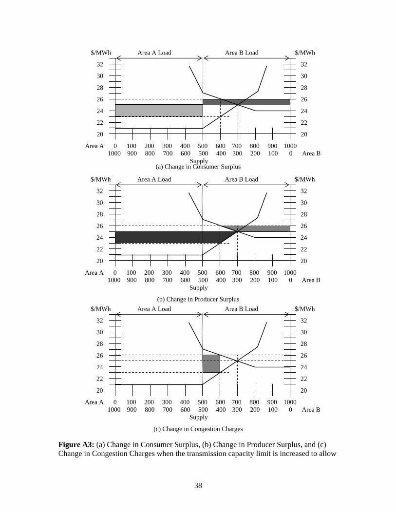
38

(a) Change in Consumer Surplus

(b) Change in Producer Surplus

(c) Change in Congestion Charges

Figure A3: (a) Change in Consumer Surplus, (b) Change in Producer Surplus, and (c) Change in Congestion Charges when the transmission capacity limit is increased to allow


20

22

24

26

28

30

32

$/MWh

20

22

24

26

28

30

32



20

22

24

26

28

30

32

$/MWh

20

22

24

26

28

30

32



20

22

24

26

28

30

32

$/MWh

20

22

24

26

28

30

32


39

uncongested operation. The light and dark shades indicate decreases and increases, respectively, in these values. Figure A4: Transfers and changes in consumer and producer surplus from an increase in transmission capacity to eliminate congestion: (A) increase in consumer surplus, (B) increase in producer surplus, (C) transfer of producer to consumer surplus, (D) transfer of consumer to producer surplus, (E) consumer surplus from congestion revenues, (F) Producer surplus from a portion of congestion revenues. In Figure A4 we detail the changes in consumer and producer surplus and the congestion revenues. The areas labeled “A” through “F” represent the following changes: A. An absolute increase in consumer surplus due to increased transmission capacity, B. An absolute increase in producer surplus due to increased transmission capacity, C. A transfer from producer surplus to consumer surplus, D. A transfer from consumer surplus to producer surplus, E. Consumer surplus from a portion of congestion revenues, and F. Producer surplus from a portion of congestion revenues. Clearly ISO policy concerning congestion revenues is important to quantify the change in consumer and producer surplus. If congestion revenues are allocated to market participants, then they add to those participants’ surplus. Then eliminating congestion will result in changes in consumer surplus and producer surplus equal to areas (A) and (B) in Figure A4. The areas corresponding to congestion charges will represent transfers of surplus between participants. It is conceivable that ISO policy might not directly allocate congestion revenues to market participants – for example, if they were saved to fund future transmission projects. Under that scenario, the congestion revenues would not contribute to the present consumer or producer surplus. The completion of such a project to eliminates congestion (perhaps funded by past congestion charges) will result


20

22

24

26

28

30

32

$/MWh

20

22

24

26

28

30

32


A

B

C D

E

F

40

in an increase in consumer and producer surpluses represented by areas (A), (B), and the congestion revenue areas (E) and (F). (The issues of ownership and rights to new transmission funded from congestion revenues would also affect these calculations and are beyond the discussion presented here.)

41

References Barmack, M., P. Griffes, E. Kahn, and S. Oren. 2003. “Performance Incentives for Transmission.” The ElectricityJournal. April 2003. pp 9-22. CAISO (California Independent System Operator). 2000. Market Analysis Reports, Jan 2000 – Dec 2000. CAISO, 2001a. Market Analysis Reports, Jan 2001 – Dec 2001. CAISO. 2001b. “Testimony of Armando J. Perez, Stephen Thomas Greenleaf and Keith Casey on behalf of the California Independent System Operator.” Path 15 CPUC Proceeding. September 25. CAISO. 2001c. Path 15 Expansion Economic Benefit Study: Phase II – Year 2005 Prospect. September 24. CAISO. 2001d. Potential Economic Benefits to California from Expanding Path 15 – Year 2005 Prospect. September 24. CAISO. 2003a. 2002 Annual Report on Market Issues and Performance. April. CAISO. 2003b. Settlements Guide. DOE (U.S. Department of Energy). 2002. National Transmission Grid Study. FERC (Federal Energy Regulatory Commission). 2001. Electric Transmission Constraint Study. Hunt, Sally. 2002. Making Competition Work in Electricity. John Wiley and Sons. ISO New England, INC. 2002a. Annual Markets Report, May 2000-April 2001, Section 2, Technical Review. September 12. ISO New England, INC. 2002b. RTEP02. November 7. Joskow, P. and J. Tirole. 2003. “Merchant Transmission Investment.” http://econ-www.mit.edu/faculty/pjoskow/papers/Merchant.pdf. Patton, D.B, and M. Wander. 2002. 2001 Annual Report on the New York Electricity Markets. June. Patton, D.B. 2003. 2002 State of the Market Report: New York Electricity Markets. April. PJM (PJM Interconnection, LLC). 2002. PJM Interconnection State of the Market Report 2001. Report of the PJM Market Monitoring Unit. June.

42

PJM. 2003. 2002 State of the Market Repor1. Report of the PJM Market Monitoring Unit. March. POWERGEM. 2002. New York Congestion and Physical Constraint Cost Estimates. Project report prepared for the New York ISO, August. Siddiqui, A., E. Bartholomew, C. Marnay, and S. Oren. 2003. The Effectiveness of Transmission Congestion Contracts in Hedging Transmission Congestion Risk in New York State. Eighth Annual Power Conference on Electric Industry Restructuring. Berkeley CA, March 14. Thomas, R.J., T.D. Mount, R.D. Zimmerman, and C. Murillo-Sanchez. 2000 “A Comparison of the Results of Three Auction Experiments.” http://www.pserc.wisc.edu/ecow/get/generalinf/presentati/presentati/ThreeAuctionsExperiment.pdf.

electricity transmission congestion costs: a review of …€¦ · · 2011-07-28lbnl-54049...

Documents