electrocardiography - pudn.comread.pudn.com/downloads138/ebook/594519/biomedical digital...

24

2

Electrocardiography

Willis J. Tompkins

One of the main techniques for diagnosing heart disease is based on the electrocar-diogram (ECG). The electrocardiograph or ECG machine permits deduction ofmany electrical and mechanical defects of the heart by measuring ECGs, which arepotentials measured on the body surface. With an ECG machine, you can deter-mine the heart rate and other cardiac parameters.

2.1 BASIC ELECTROCARDIOGRAPHY

There are three basic techniques used in clinical electrocardiography. The mostfamiliar is the standard clinical electrocardiogram. This is the test done in a physi-cian’s office in which 12 different potential differences called ECG leads arerecorded from the body surface of a resting patient. A second approach uses an-other set of body surface potentials as inputs to a three-dimensional vector modelof cardiac excitation. This produces a graphical view of the excitation of the heartcalled the vectorcardiogram (VCG). Finally, for long-term monitoring in the inten-sive care unit or on ambulatory patients, one or two ECG leads are monitored orrecorded to look for life-threatening disturbances in the rhythm of the heartbeat.This approach is called arrhythmia analysis. Thus, the three basic techniques usedin electrocardiography are:

1. Standard clinical ECG (12 leads)2. VCG (3 orthogonal leads)3. Monitoring ECG (1 or 2 leads)

Figure 2.1 shows the basic objective of electrocardiography. By looking at elec-trical signals recorded only on the body surface, a completely noninvasive proce-dure, cardiologists attempt to determine the functional state of the heart. Althoughthe ECG is an electrical signal, changes in the mechanical state of the heart lead tochanges in how the electrical excitation spreads over the surface of the heart,thereby changing the body surface ECG. The study of cardiology is based on therecording of the ECGs of thousands of patients over many years and observing the

Electrocardiography 25

relationships between various waveforms in the signal and different abnormalities.Thus clinical electrocardiography is largely empirical, based mostly on experientialknowledge. A cardiologist learns the meanings of the various parts of the ECG sig-nal from experts who have learned from other experts.

Condition of the heart

Body surface potentials

(electrocardiograms)

Empirical

Figure 2.1 The object of electrocardiography is to deduce the electrical and mechanicalcondition of the heart by making noninvasive body surface potential measurements.

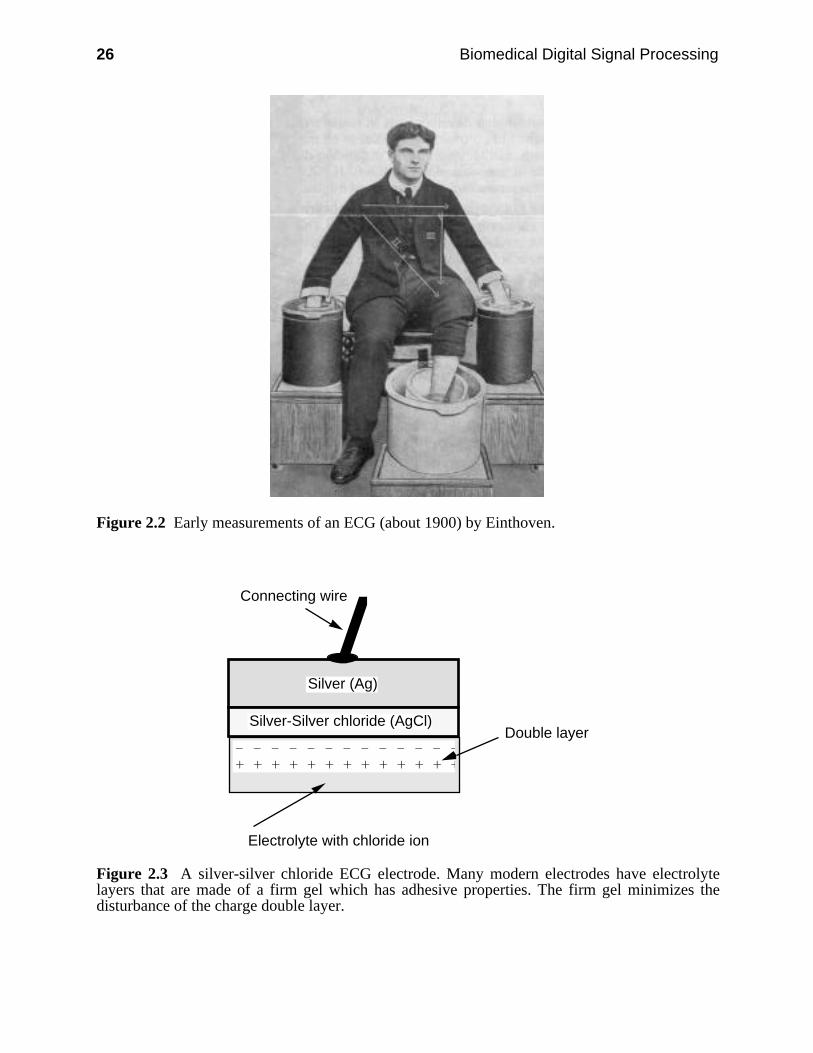
Figure 2.2 shows how the earliest ECGs were recorded by Einthoven at aroundthe turn of the century. Vats of salt water provided the electrical connection to thebody. The string galvanometer served as the measurement instrument for recordingthe ECG.

2.1.1 Electrodes

As time went on, metallic electrodes were developed to electrically connect to thebody. An electrolyte, usually composed of salt solution in a gel, forms the electri-cal interface between the metal electrode and the skin. In the body, currents areproduced by movement of ions whereas in a wire, currents are due to the move-ment of electrons. Electrode systems do the conversion of ionic currents to electroncurrents.

Conductive metals such as nickel-plated brass are used as ECG electrodes butthey have a problem. The two electrodes necessary to acquire an ECG togetherwith the electrolyte and the salt-filled torso act like a battery. A dc offset potentialoccurs across the electrodes that may be as large or larger than the peak ECGsignal. A charge double layer (positive and negative ions separated by a distance)occurs in the electrolyte. Movement of the electrode such as that caused by motionof the patient disturbs this double layer and changes the dc offset. Since this offsetpotential is amplified about 1,000 times along with the ECG, small changes giverise to large baseline shifts in the output signal. An electrode that behaves in thisway is called a polarizable electrode and is only useful for resting patients.

26 Biomedical Digital Signal Processing

Figure 2.2 Early measurements of an ECG (about 1900) by Einthoven.

Silver (Ag)

Silver-Silver chloride (AgCl)

Connecting wire

– – – – – – – – – – – – – + + + + + + + + + + + + +

Electrolyte with chloride ion

Double layer

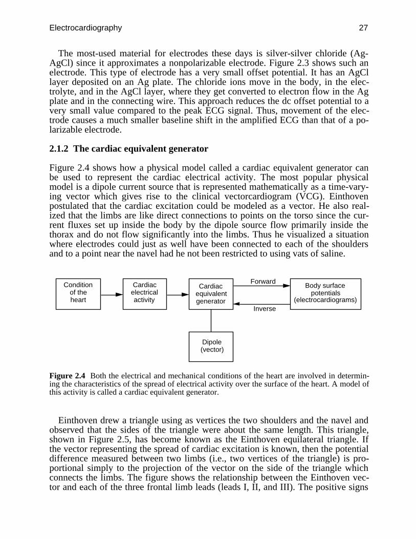
Figure 2.3 A silver-silver chloride ECG electrode. Many modern electrodes have electrolytelayers that are made of a firm gel which has adhesive properties. The firm gel minimizes thedisturbance of the charge double layer.


The most-used material for electrodes these days is silver-silver chloride (Ag-AgCl) since it approximates a nonpolarizable electrode. Figure 2.3 shows such anelectrode. This type of electrode has a very small offset potential. It has an AgCllayer deposited on an Ag plate. The chloride ions move in the body, in the elec-trolyte, and in the AgCl layer, where they get converted to electron flow in the Agplate and in the connecting wire. This approach reduces the dc offset potential to avery small value compared to the peak ECG signal. Thus, movement of the elec-trode causes a much smaller baseline shift in the amplified ECG than that of a po-larizable electrode.

2.1.2 The cardiac equivalent generator

Figure 2.4 shows how a physical model called a cardiac equivalent generator canbe used to represent the cardiac electrical activity. The most popular physicalmodel is a dipole current source that is represented mathematically as a time-vary-ing vector which gives rise to the clinical vectorcardiogram (VCG). Einthovenpostulated that the cardiac excitation could be modeled as a vector. He also real-ized that the limbs are like direct connections to points on the torso since the cur-rent fluxes set up inside the body by the dipole source flow primarily inside thethorax and do not flow significantly into the limbs. Thus he visualized a situationwhere electrodes could just as well have been connected to each of the shouldersand to a point near the navel had he not been restricted to using vats of saline.

Condition of the heart

Body surface potentials

(electrocardiograms)

Cardiac electrical activity

Cardiac equivalent generator

Dipole (vector)

Forward

Inverse

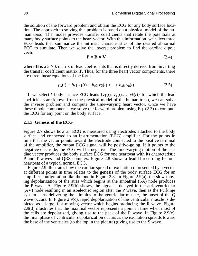
Figure 2.4 Both the electrical and mechanical conditions of the heart are involved in determin-ing the characteristics of the spread of electrical activity over the surface of the heart. A model ofthis activity is called a cardiac equivalent generator.

Einthoven drew a triangle using as vertices the two shoulders and the navel andobserved that the sides of the triangle were about the same length. This triangle,shown in Figure 2.5, has become known as the Einthoven equilateral triangle. Ifthe vector representing the spread of cardiac excitation is known, then the potentialdifference measured between two limbs (i.e., two vertices of the triangle) is pro-portional simply to the projection of the vector on the side of the triangle whichconnects the limbs. The figure shows the relationship between the Einthoven vec-tor and each of the three frontal limb leads (leads I, II, and III). The positive signs


show which connection goes to the positive input of the instrumentation amplifierfor each lead.

+

++

I

IIIII

LARA

LL

Figure 2.5 Einthoven equilateral triangle. RA and LA are the right and left arms and LL is theleft leg.

A current dipole is a current source and a current sink separated by a distance.Since such a dipole has magnitude and direction which change throughout aheartbeat as the cells in the heart depolarize, this leads to the vector representation

p(t) = px(t) x + py(t) y + pz(t) z (2.1)

where p(t) is the time-varying cardiac vector, pi(t) are the orthogonal componentsof the vector also called scalar leads, and x , y , z are unit vectors in the x, y, zdirections.

A predominant VCG researcher in the 1950s named Frank shaped a plaster castof a subject’s body like the one shown in Figure 2.6, waterproofed it, and filled itwith salt water. He placed a dipole source composed of a set of two electrodes on astick in the torso model at the location of the heart. A current source suppliedcurrent to the electrodes which then produced current fluxes in the volumeconductor. From electrodes embedded in the plaster, Frank measured the bodysurface potential distribution at many thoracic points resulting from the currentsource. From the measurements in such a study, he found the geometrical transfercoefficients that relate the dipole source to each of the body surface potentials.


i

Torso model

Torso surface recording electrode

Dipole current source electrode

Saline solution

Figure 2.6 Torso model used to develop the Frank lead system for vectorcardiography.

Once the transfer coefficients are known, the forward problem of electrocardiog-raphy can be solved for any dipole source. The forward solution provides the po-tential at any arbitrary point on the body surface for a given cardiac dipole.Expressed mathematically,

vn(t) = tnx px(t) + tny py(t) + tnz pz(t) (2.2)

This forward solution shows that the potential vn(t) (i.e., the ECG) at any point non the body surface is given by the linear sum of the products of a set of transfercoefficients [tni] unique to that point and the corresponding orthogonal dipole vec-tor components [pi(t)]. The ECGs are time varying as are the dipole components,while the transfer coefficients are only dependent on the thoracic geometry and in-homogeneities. Thus for a set of k body surface potentials (i.e., leads), there is a setof k equations that can be expressed in matrix form

V = T × P (2.3)

where V is a k × 1 vector representing the time-varying potentials, T is a k × 3 ma-trix of transfer coefficients, which are fixed for a given individual, and P is the3 × 1 time-varying heart vector.

Of course, the heart vector and transfer coefficients are unknown for a given in-dividual. However if we had a way to compute this heart vector, we could use it in


the solution of the forward problem and obtain the ECG for any body surface loca-tion. The approach to solving this problem is based on a physical model of the hu-man torso. The model provides transfer coefficients that relate the potentials atmany body surface points to the heart vector. With this information, we select threeECG leads that summarize the intrinsic characteristics of the desired abnormalECG to simulate. Then we solve the inverse problem to find the cardiac dipolevector

P = B × V (2.4)

where B is a 3 × k matrix of lead coefficients that is directly derived from invertingthe transfer coefficient matrix T. Thus, for the three heart vector components, thereare three linear equations of the form

px(t) = bx1 v1(t) + bx2 v2(t) +…+ bxk vk(t) (2.5)

If we select k body surface ECG leads v1(t), v2(t),…, vk(t) for which the leadcoefficients are known from the physical model of the human torso, we can solvethe inverse problem and compute the time-varying heart vector. Once we havethese dipole components, we solve the forward problem using Eq. (2.3) to computethe ECG for any point on the body surface.

2.1.3 Genesis of the ECG

Figure 2.7 shows how an ECG is measured using electrodes attached to the bodysurface and connected to an instrumentation (ECG) amplifier. For the points intime that the vector points toward the electrode connected to the positive terminalof the amplifier, the output ECG signal will be positive-going. If it points to thenegative electrode, the ECG will be negative. The time-varying motion of the car-diac vector produces the body surface ECG for one heartbeat with its characteristicP and T waves and QRS complex. Figure 2.8 shows a lead II recording for oneheartbeat of a typical normal ECG.

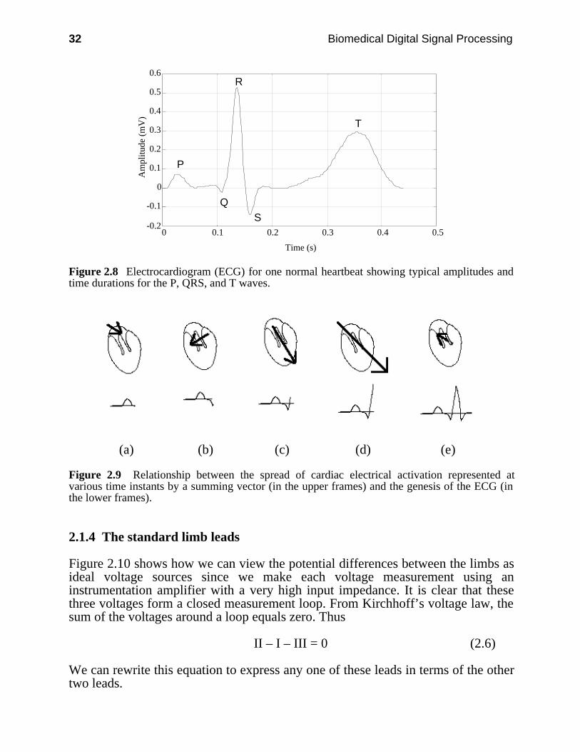
Figure 2.9 illustrates how the cardiac spread of excitation represented by a vectorat different points in time relates to the genesis of the body surface ECG for anamplifier configuration like the one in Figure 2.8. In Figure 2.9(a), the slow-mov-ing depolarization of the atria which begins at the sinoatrial (SA) node producesthe P wave. As Figure 2.9(b) shows, the signal is delayed in the atrioventricular(AV) node resulting in an isoelectric region after the P wave, then as the Purkinjesystem starts delivering the stimulus to the ventricular muscle, the onset of the Qwave occurs. In Figure 2.9(c), rapid depolarization of the ventricular muscle is de-picted as a large, fast-moving vector which begins producing the R wave. Figure2.9(d) illustrates that the maximal vector represents a point in time when most ofthe cells are depolarized, giving rise to the peak of the R wave. In Figure 2.9(e),the final phase of ventricular depolarization occurs as the excitation spreads towardthe base of the ventricles (to the top in the picture) giving rise to the S wave.


(a)

Torso

P

Q

R

S

T

(b)

Figure 2.7 Basic configuration for recording an electrocardiogram. Using electrodes attached tothe body, the ECG is recorded with an instrumentation amplifier. (a) Transverse (top) view of aslice of the body showing the heart and lungs. (b) Frontal view showing electrodes connected inan approximate lead II configuration.


-0.2

-0.1

0

0.1

0.2

0.3

0.4

0.5

0.6

0 0.1 0.2 0.3 0.4 0.5

Time (s)

Am

plitu

de (

mV

)

P

Q

R

S

T

Figure 2.8 Electrocardiogram (ECG) for one normal heartbeat showing typical amplitudes andtime durations for the P, QRS, and T waves.

(a) (b) (c) (d) (e)

Figure 2.9 Relationship between the spread of cardiac electrical activation represented atvarious time instants by a summing vector (in the upper frames) and the genesis of the ECG (inthe lower frames).

2.1.4 The standard limb leads

Figure 2.10 shows how we can view the potential differences between the limbs asideal voltage sources since we make each voltage measurement using aninstrumentation amplifier with a very high input impedance. It is clear that thesethree voltages form a closed measurement loop. From Kirchhoff’s voltage law, thesum of the voltages around a loop equals zero. Thus

II – I – III = 0 (2.6)

We can rewrite this equation to express any one of these leads in terms of the othertwo leads.


II = I + III (2.7a)

I = II – III (2.7b)

III = II – I (2.7c)

It is thus clear that one of these voltages is completely redundant; we canmeasure any two and compute the third. In fact, that is exactly what modern ECGmachines do. Most machines measure leads I and II and compute lead III. Youmight ask why we even bother with computing lead III; it is redundant so it has nonew information not contained in leads I and II. For the answer to this question, weneed to go back to Figure 2.1 and recall that cardiologists learned the relationshipsbetween diseases and ECGs by looking at a standard set of leads and relating theappearance of each to different abnormalities. Since these three leads were selectedin the beginning, the appearance of each of them is important to the cardiologist.

+

++

I

IIIII

LARA

LL

Figure 2.10 Leads I, II, and III are the potential differences between the limbs as indicated. RAand LA are the right and left arms and LL is the left leg.

2.1.5 The augmented limb leads

The early instrumentation had inadequate gain to produce large enough ECG tracesfor all subjects, so the scheme in Figure 2.11 was devised to produce larger ampli-tude signals. In this case, the left arm signal, called augmented limb lead aVL, ismeasured using the average of the potentials on the other two limbs as a reference.


We can analyze this configuration using standard circuit theory. From the bot-tom left loop

i × R + i × R – II = 0 (2.8)or

i × R = II2 (2.9)

From the bottom right loop–i × R + III + aVL = 0 (2.10)

oraVL = i × R – III (2.11)

Combining Eqs. (2.9) and (2.11) gives

aVL = II2 – III =

II – 2 × III2 (2.12)

+

++

I

IIIII

LARA

LL R

R

+

–aVL

i

Figure 2.11 The augmented limb lead aVL is measured as shown.


LARA

LL R

R

(a)

R

R

(b)

R/2

(c)

Figure 2.12 Determination of the Thévenin resistance for the aVL equivalent circuit. (a) Allideal voltage sources are shorted out. (b) This gives rise to the parallel combination of two equalresistors. (c) The Thévenin equivalent resistance thus has a value of R/2.


From the top center loopII = III + I (2.13)

Substituting gives

aVL = III + I – 2 × III

2 = I – III

2 (2.14)

This is the Thévenin equivalent voltage for the augmented lead aVL as an aver-age of two of the frontal limb leads. It is clear that aVL is a redundant lead since itcan be expressed in terms of two other leads. The other two augmented leads, aVRand aVF, similarly can both be expressed as functions of leads I and III. Thus herewe find an additional three leads, all of which can be calculated from two of thefrontal leads and thus are all redundant with no new real information. However dueto the empirical nature of electrocardiology, the physician nonetheless still needs tosee the appearance of these leads to facilitate the diagnosis.

Figure 2.12 shows how the Thévenin equivalent resistance is found by shortingout the ideal voltage sources and looking back from the output terminals.

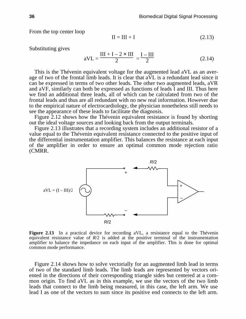
Figure 2.13 illustrates that a recording system includes an additional resistor of avalue equal to the Thévenin equivalent resistance connected to the positive input ofthe differential instrumentation amplifier. This balances the resistance at each inputof the amplifier in order to ensure an optimal common mode rejection ratio(CMRR.

+

–

R/2

R/2

+

–

aVL = (I – III)/2

Figure 2.13 In a practical device for recording aVL, a resistance equal to the Théveninequivalent resistance value of R/2 is added at the positive terminal of the instrumentationamplifier to balance the impedance on each input of the amplifier. This is done for optimalcommon mode performance.

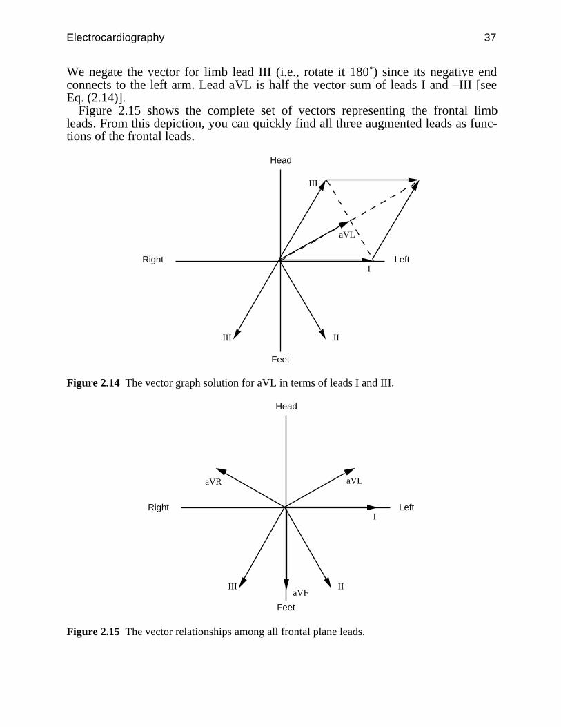
Figure 2.14 shows how to solve vectorially for an augmented limb lead in termsof two of the standard limb leads. The limb leads are represented by vectors ori-ented in the directions of their corresponding triangle sides but centered at a com-mon origin. To find aVL as in this example, we use the vectors of the two limbleads that connect to the limb being measured, in this case, the left arm. We uselead I as one of the vectors to sum since its positive end connects to the left arm.


We negate the vector for limb lead III (i.e., rotate it 180˚) since its negative endconnects to the left arm. Lead aVL is half the vector sum of leads I and –III [seeEq. (2.14)].

Figure 2.15 shows the complete set of vectors representing the frontal limbleads. From this depiction, you can quickly find all three augmented leads as func-tions of the frontal leads.

I

IIIII

–III

aVL

Head

Feet

LeftRight

Figure 2.14 The vector graph solution for aVL in terms of leads I and III.

I

IIIII

aVL

Head

Feet

LeftRight

aVR

aVF

Figure 2.15 The vector relationships among all frontal plane leads.


+

–I

LARA

RL LL +

–

LARA

RL LL

R

R/2

R aVR

(a) (d)

+

–

II

LARA

RL LL

+

–

LARA

RL LL

R

R/2

R

aVL

(b) (e)

+

–III

LARA

RL LL+

–

LARA

RL LL

R

R/2

R aVF

(c) (f)

LARA

RL LL

+

–

R

RV Leads

R

R/3

Wilson's central terminal

(g)Figure 2.16 Standard 12-lead clinical electrocardiogram. (a) Lead I. (b) Lead II. (c) Lead III.Note the amplifier polarity for each of these limb leads. (d) aVR. (e) aVL. (f) aVF. These aug-mented leads require resistor networks which average two limb potentials while recording thethird. (g) The six V leads are recorded referenced to Wilson’s central terminal which is the aver-age of all three limb potentials. Each of the six leads labeled V1–V6 are recorded from a differ-ent anatomical site on the chest.


2.2 ECG LEAD SYSTEMS

There are three basic lead systems used in cardiology. The most popular is the 12-lead approach, which defines the set of 12 potential differences that make up thestandard clinical ECG. A second lead system designates the locations of electrodesfor recording the VCG. Monitoring systems typically analyze one or two leads.

2.2.1 12-lead ECG

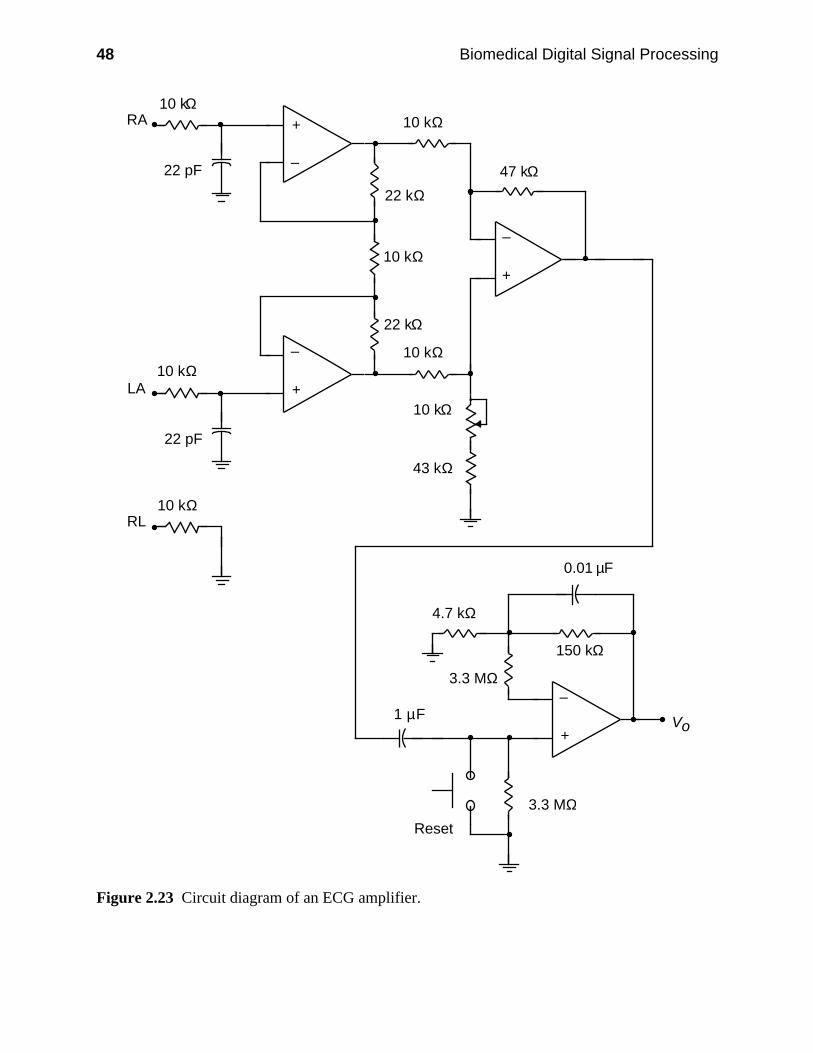
Figure 2.16 shows how the 12 leads of the standard clinical ECG are recorded, andFigure 2.17 shows the standard 12-lead ECG for a normal patient. The instrumen-tation amplifier is a special design for electrocardiography like the one shown inFigure 2.23. In modern microprocessor-based ECG machines, there are eight simi-lar ECG amplifiers which simultaneously record leads I, II, and V1–V6. They thencompute leads III, aVL, aVR, and aVF for the final report.

Figure 2.17 The 12-lead ECG of a normal male patient. Calibration pulses on the left sidedesignate 1 mV. The recording speed is 25 mm/s. Each minor division is 1 mm, so the majordivisions are 5 mm. Thus in lead I, the R-wave amplitude is about 1.1 mV and the time betweenbeats is almost 1 s (i.e., heart rate is about 60 bpm).


2.2.2 The vectorcardiogram

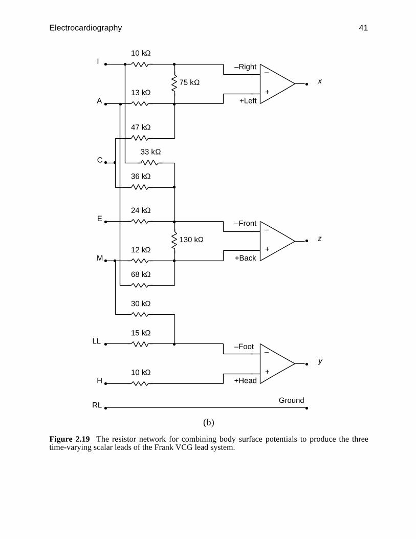
Figure 2.18 illustrates the placement of electrodes for a Frank VCG lead system.Worldwide this is the most popular VCG lead system. Figure 2.19 shows howpotentials are linearly combined with a resistor network to compute the three time-varying orthogonal scalar leads of the Frank lead system. Figure 2.20 is an IBMPC screen image of the VCG of a normal patient.

LL

x

z

y

RL

H

I

E CA

M

Figure 2.18 The electrode placement for the Frank VCG lead system.


+

–

10 kΩ

13 kΩ

68 kΩ

30 kΩ

47 kΩ

33 kΩ

36 kΩ

75 kΩ

+

–

24 kΩ

12 kΩ 130 kΩ

+

–

15 kΩ

10 kΩ

–Right

+Left

–Front

+Back

–Foot

+Head

Ground

I

A

C

E

M

LL

H

RL

x

z

y

(b)

Figure 2.19 The resistor network for combining body surface potentials to produce the threetime-varying scalar leads of the Frank VCG lead system.


Figure 2.20 The vectorcardiogram of a normal male patient. The three time-varying scalar leadsfor one heartbeat are shown on the left and are the x, y, and z leads from top to bottom. In the topcenter is the frontal view of the tip of the vector as it moves throughout one complete heartbeat.In bottom center is a transverse view of the vector loop looking down from above the patient. Onthe far right is a left sagittal view looking toward the left side of the patient.

2.2.3 Monitoring lead systems

Monitoring applications do not use standard electrode positions but typically usetwo leads. Since the principal goal of these systems is to reliably recognize eachheartbeat and perform rhythm analysis, electrodes are placed so that the primaryECG signal has a large R-wave amplitude. This ensures a high signal-to-noise ratiofor beat detection. Since Lead II has a large peak amplitude for many patients, thislead is frequently recommended as the first choice of a primary lead by manymanufacturers. A secondary lead with different electrode placements serves as abackup in case the primary lead develops problems such as loss of electrodecontact.


2.3 ECG SIGNAL CHARACTERISTICS

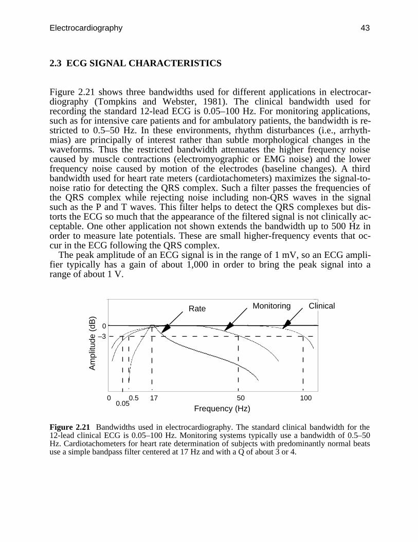
Figure 2.21 shows three bandwidths used for different applications in electrocar-diography (Tompkins and Webster, 1981). The clinical bandwidth used forrecording the standard 12-lead ECG is 0.05–100 Hz. For monitoring applications,such as for intensive care patients and for ambulatory patients, the bandwidth is re-stricted to 0.5–50 Hz. In these environments, rhythm disturbances (i.e., arrhyth-mias) are principally of interest rather than subtle morphological changes in thewaveforms. Thus the restricted bandwidth attenuates the higher frequency noisecaused by muscle contractions (electromyographic or EMG noise) and the lowerfrequency noise caused by motion of the electrodes (baseline changes). A thirdbandwidth used for heart rate meters (cardiotachometers) maximizes the signal-to-noise ratio for detecting the QRS complex. Such a filter passes the frequencies ofthe QRS complex while rejecting noise including non-QRS waves in the signalsuch as the P and T waves. This filter helps to detect the QRS complexes but dis-torts the ECG so much that the appearance of the filtered signal is not clinically ac-ceptable. One other application not shown extends the bandwidth up to 500 Hz inorder to measure late potentials. These are small higher-frequency events that oc-cur in the ECG following the QRS complex.

The peak amplitude of an ECG signal is in the range of 1 mV, so an ECG ampli-fier typically has a gain of about 1,000 in order to bring the peak signal into arange of about 1 V.

0

0

50 100

Frequency (Hz)

Am

plitu

de (

dB)

MonitoringRate

170.05

0.5

–3

Clinical

Figure 2.21 Bandwidths used in electrocardiography. The standard clinical bandwidth for the12-lead clinical ECG is 0.05–100 Hz. Monitoring systems typically use a bandwidth of 0.5–50Hz. Cardiotachometers for heart rate determination of subjects with predominantly normal beatsuse a simple bandpass filter centered at 17 Hz and with a Q of about 3 or 4.


2.4 LAB: ANALOG FILTERS, ECG AMPLIFIER, AND QRS DETECTOR*

In this laboratory you will study the characteristics of four types of analog filters:low-pass, high-pass, bandpass and bandstop. You will use these filters to build anECG amplifier. Next you will study the application of a bandpass filter in a QRSdetector circuit, which produces a pulse for each occurrence of a QRS complex.Note that you have to build all the circuits yourself.

2.4.1 Equipment

1. Dual trace oscilloscope2. Signal generator3. ECG electrodes4. Chart recorder5. Your ECG amplifier and QRS detection board6. Your analog filter board

2.4.2 Background information

Low-pass filter/integrator

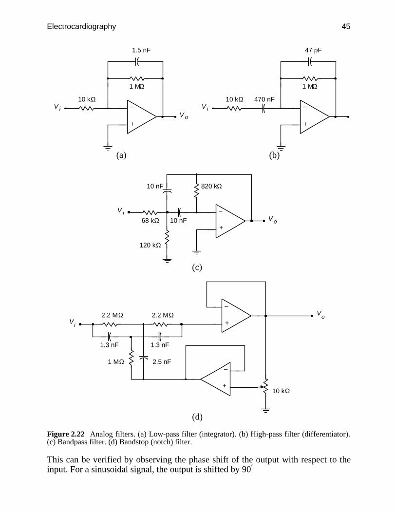
Figure 2.22(a) shows the circuit for a low-pass filter. The low-frequency gain, AL,is given by

AL = – R2 R1

(2.15)

The negative sign results because the op amp is in an inverting amplifier configura-tion. The high-corner frequency is given by

fh = 1

2πR2C1 (2.16)

A low-pass filter acts like an integrator at high frequencies. The integrator output isgiven by

V0= – 1

1 + j R1C1 Vi

= – 1

R1C1 ∫ Vi dt (2.17)

* Section 2.4 was written by Pradeep Tagare.


+

–10 kΩ

1 MΩ

1.5 nF

oViV

+

–10 kΩ

1 MΩ

47 pF

iV470 nF

(a) (b)

+

–

68 kΩ oViV

10 nF

820 kΩ10 nF

120 kΩ

(c)

+

–2.2 MΩ o

V

iV

1.3 nF

1 MΩ 2.5 nF

10 kΩ+

–

2.2 MΩ

1.3 nF

(d)

Figure 2.22 Analog filters. (a) Low-pass filter (integrator). (b) High-pass filter (differentiator).(c) Bandpass filter. (d) Bandstop (notch) filter.

This can be verified by observing the phase shift of the output with respect to theinput. For a sinusoidal signal, the output is shifted by 90˚


⌡⌠ v sin t = – v

cos t = v

sin( t + π2 ) (2.18)

Thus the gain of the integrator falls at high frequencies. Also note that if R2 werenot included in the integrator, the gain would become infinite at dc. Thus at dc theop amp dc bias current charges the integrating capacitor C1 and saturates theamplifier.

High-pass filter/differentiator

In contrast to the low-pass filter which acts as an integrator at high frequencies, thehigh-pass filter acts like a differentiator at low frequencies. Referring to Figure2.22(b), we get the high-frequency gain Ah and the low-corner frequency fL as

Ah = – R2 R1

(2.19)

fL = 1

2πR1C1 (2.20)

The differentiating behavior of the high-pass filter at low frequencies can be veri-fied by deriving equations as was done for the integrator. Capacitor C2 is added toimprove the stability of the differentiator. The differentiator gain increases withfrequency, up to the low-corner frequency.

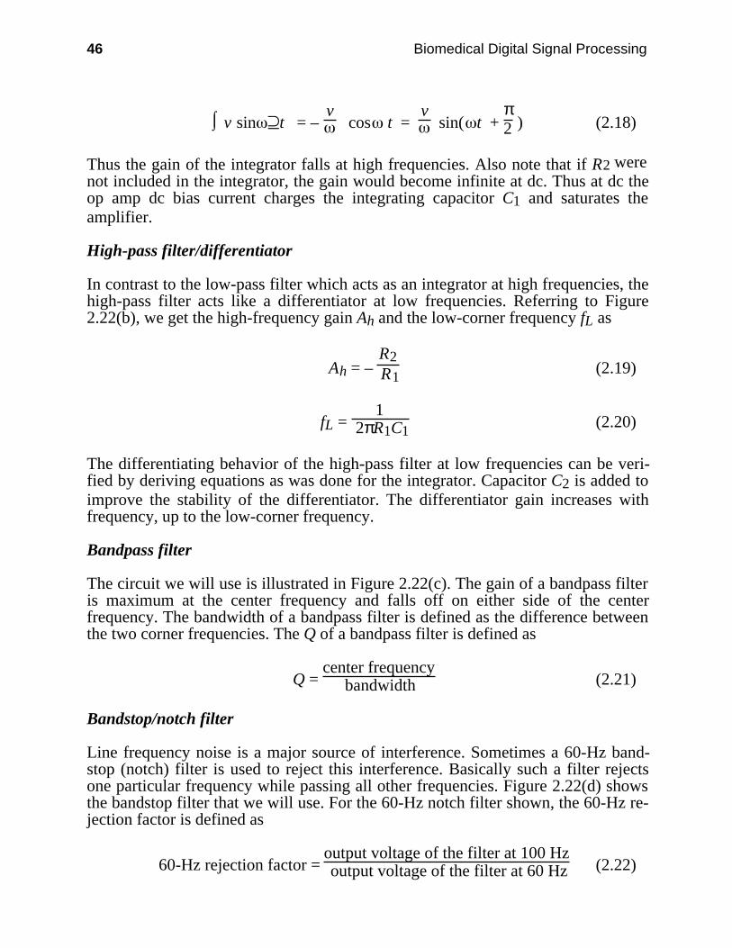
Bandpass filter

The circuit we will use is illustrated in Figure 2.22(c). The gain of a bandpass filteris maximum at the center frequency and falls off on either side of the centerfrequency. The bandwidth of a bandpass filter is defined as the difference betweenthe two corner frequencies. The Q of a bandpass filter is defined as

Q = center frequency

bandwidth (2.21)

Bandstop/notch filter

Line frequency noise is a major source of interference. Sometimes a 60-Hz band-stop (notch) filter is used to reject this interference. Basically such a filter rejectsone particular frequency while passing all other frequencies. Figure 2.22(d) showsthe bandstop filter that we will use. For the 60-Hz notch filter shown, the 60-Hz re-jection factor is defined as

60-Hz rejection factor = output voltage of the filter at 100 Hz output voltage of the filter at 60 Hz (2.22)


for the same input voltage.

ECG amplifier

An ECG signal is usually in the range of 1 mV in magnitude and has frequencycomponents from about 0.05–100 Hz. To process this signal, it has to be amplified.Figure 2.23 shows the circuit of an ECG amplifier. The typical characteristics of anECG amplifier are high gain (about 1,000), 0.05–100 Hz frequency response, highinput impedance, and low output impedance. Derivation of equations for the gainand frequency response are left as an exercise for the reader.

QRS detector

Figures 2.24 and 2.25 show the block diagram and complete schematic for theQRS detector. The QRS detector consists of the following five units:

1. QRS filter. The power spectrum of a normal ECG signal has the greatest signal-to-noise ratio at about 17 Hz. Therefore to detect the QRS complex, the ECG ispassed through a bandpass filter with a center frequency of 17 Hz and a band-width of 6 Hz. This filter has a large amount of ringing in its output.

2. Half-wave rectifier. The filtered QRS is half-wave rectified, to be subsequentlycompared with a threshold voltage generated by the detector circuit.

3. Threshold circuit. The peak voltage of the rectified and filtered ECG is storedon a capacitor. A fraction of this voltage (threshold voltage) is compared withthe filtered and rectified ECG output.

4. Comparator. The QRS pulse is detected when the threshold voltage is exceeded.The capacitor recharges to a new threshold voltage after every pulse. Hence anew threshold determined from the past history of the signal is generated afterevery pulse.

5. Monostable. A 200-ms pulse is generated for every QRS complex detected.This pulse drives a LED.

Some patients have a cardiac pacemaker. Since sharp pulses of the pacemakercan cause spurious QRS pulse detection, a circuit is often included to reject pace-maker pulses. The rejection is achieved by limiting the slew rate of the amplifier.


+

–

+

–

+

–

+

–

43 kΩ

10 kΩ

10 kΩ

10 kΩ

22 pF

10 kΩ

10 kΩ

10 kΩ

22 kΩ

22 kΩ

47 kΩ

4.7 kΩ

150 kΩ

1 µF

3.3 MΩ

Vo

RA

LA

RL10 kΩ

22 pF

Reset

0.01 µF

3.3 MΩ

Figure 2.23 Circuit diagram of an ECG amplifier.


ECG amplifier

QRS filter

Threshold circuit Comparator Monostable

TP1 TP2 TP3

Half-wave rectifier

TP6TP5TP4

Figure 2.24 Block diagram of a QRS detector.

+

–

68 kΩ 470 nF

820 kΩ470 nF

120 kΩ

470 nF

ECG IN

820 kΩ

TP1

100 kΩ

TP2

+

–

100 kΩ

+

– +

–

820 kΩ

330 kΩ

1 µF

TP3

TP4

TP5

QRS OUT

TP6

10 nF

+5 V

+5 V

1.8 µF

+

100 kΩ

16,7

34,82

5

5551 kΩ

Figure 2.25 QRS detector circuit.


2.4.3 Experimental Procedure

Build all the circuits described above using the LM324 quad operational amplifierintegrated circuit shown in Figure 2.26.

2 3 4 5 6 7

8910111214 13

+ +

++

+5 V

Gnd

1––

––

Figure 2.26 Pinout of the LM324 quad operational amplifier integrated circuit.

Low-pass filter

1. Turn on the power to the filter board. Feed a sinusoidal signal of the least pos-sible amplitude generated by the signal generator at 10 Hz into the integratorinput and observe both the input and the output on the oscilloscope. Calculatethe gain.

2. Starting with a frequency of 10 Hz, increase the signal frequency in steps of 10Hz up to 200 Hz and record the output at each frequency. You will use thesevalues to plot a graph of the output voltage versus frequency. Next, find thegenerator frequency for which the output is 0.707-times that observed at 10 Hz.This is the –3 dB point or the high-corner frequency. Record this value.

3. Verify the operation of a low-pass filter as an integrator at high frequencies byobserving the phase shift between the input and the output. Record the phaseshift at the high-corner frequency.

High-pass filter

1. Feed a sinusoidal signal of the least possible amplitude generated by the signalgenerator at 200 Hz into the differentiator input and observe both the input andthe output on the oscilloscope. Calculate the gain.

2. Starting with a frequency of 200 Hz, decrease the signal frequency in steps of20 Hz to near dc and record the output at each frequency. You will use thesevalues to plot a graph of the output voltage versus frequency. Next find the gen-erator frequency for which the output is 0.707-times that observed at 200 Hz.This is the 3 dB point or the low-corner frequency. Record this value.


3. Verify the operation of a high-pass filter as a differentiator at low frequenciesby observing the phase shift between the input and the output. Record the phaseshift at the low-corner frequency. Another simple way to observe the differenti-ating behavior is to feed a 10-Hz square wave into the input and observe thespikes at the output.

Bandpass filter

For a 1-V p-p sinusoidal signal, vary the frequency from 10–150 Hz. Record thehigh- and low-corner frequencies. Find the center frequency and the passbandgain of this filter.

Bandstop/notch filter

Feed a 1-V p-p 60-Hz sinusoidal signal into the filter, and measure the outputvoltage. Repeat the same for a 100-Hz sinusoid. Record results.

ECG amplifier

1. Connect LA and RA inputs of the amplifier to ground and observe the output.Adjust the 100-kΩ pot to null the offset voltage.

2. Connect LA and RA inputs to the signal high and the RL input to signal high(60 Hz) and RL to signal low. This is the common mode operation. Calculatethe common mode gain.

3. Connect the LA input to the signal high (30 Hz) and the RA input to the signallow (through an attenuator to avoid saturation). This is the differential modeoperation. Calculate the differential mode gain.

4. Find the frequency response of the amplifier.5. Connect three electrodes to your body. Connect these electrodes to the amplifier

inputs. Observe the amplifier output. If the signal is very noisy, try twisting theleads together. When you get a good signal, get a recording on the chartrecorder.

QRS detector

1. Apply three ECG electrodes. Connect the electrodes to the input of the ECGamplifier board. Turn on the power to the board and observe the output of theECG amplifier on the oscilloscope. Try pressing the electrodes if there is ex-cessive noise.

2. Connect the output of the ECG amplifier to the input of the QRS detector board.Observe the following signals on the oscilloscope and then record them on astripchart recorder with the ECG (TP1) on one channel and each of the othertest signals (TP2–TP6) on the other channel. Use a reasonably fast paper speed(e.g., 25 mm/s).


Signals to be observed:

Test point Signal

TP1 Your ECGTP2 Filtered outputTP3 Rectified outputTP4 Comparator inputTP5 Comparator outputTP6 Monostable output

The LED should flash for every QRS pulse detected.

2.4.4 Lab report

1. Using equations described in the text, determine the values of AL and fh for thelow-pass filter. Compare these values with the respective values obtained inthe lab and account for any differences.

2. Plot the graph of the filter output voltage versus frequency. Show the –3 dBpoint on this graph.

3. What value of phase shift did you obtain for the low-pass filter?4. Using equations described in the text, determine the values of AH and fL for

the high-pass filter. Compare these values with the respective values obtainedin the lab and account for any differences.

5. Plot the graph of the filter output voltage versus frequency. Show the –3 dBpoint on this graph.

6. What value of phase shift did you obtain for the high-pass filter?7. For the bandpass amplifier, list the values that you got for the following:

(a) center frequency(b) passband gain(c) bandwidth(d) QShow all calculations.

8. What is the 60-Hz rejection factor for the bandstop filter you used?9. What are the upper and lower –3 dB frequencies of your ECG amplifier? How

do they compare with the theoretical values?10. What is the gain of your ECG amplifier? How does it compare with the

theoretical value?11. What is the CMRR of your ECG amplifier?12. How would you change the –3 dB frequencies of this amplifier?13. Explain the waveforms you recorded on the chart recorder. Are these what

you would expect to obtain?14. Will the QRS detector used in this lab work for any person’s ECG? Justify

your answer.

Include all chart recordings with your lab report and show calculations whereverappropriate.


2.5 REFERENCES

Tompkins, W. J. and Webster, J. G. (eds.) 1981. Design of Microcomputer-based MedicalInstrumentation. Englewood Cliffs, NJ: Prentice-Hall.

2.6 STUDY QUESTIONS

2.1 What is a cardiac equivalent generator? How is it different from the actual cardiac electricalactivity? Give two examples.

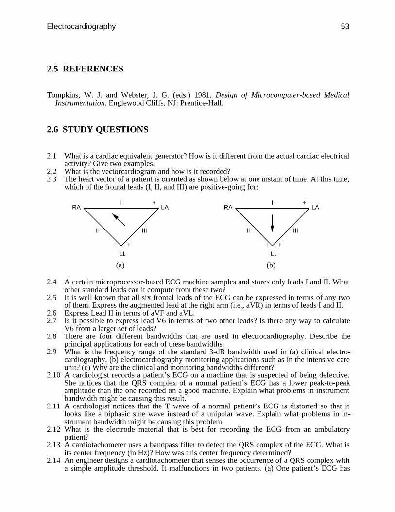
2.2 What is the vectorcardiogram and how is it recorded?2.3 The heart vector of a patient is oriented as shown below at one instant of time. At this time,

which of the frontal leads (I, II, and III) are positive-going for:

II

I

III

+ +

+RA LA

LL

II

I

III

+ +

+RA LA

LL

(a) (b)

2.4 A certain microprocessor-based ECG machine samples and stores only leads I and II. Whatother standard leads can it compute from these two?

2.5 It is well known that all six frontal leads of the ECG can be expressed in terms of any twoof them. Express the augmented lead at the right arm (i.e., aVR) in terms of leads I and II.

2.6 Express Lead II in terms of aVF and aVL.2.7 Is it possible to express lead V6 in terms of two other leads? Is there any way to calculate

V6 from a larger set of leads?2.8 There are four different bandwidths that are used in electrocardiography. Describe the

principal applications for each of these bandwidths.2.9 What is the frequency range of the standard 3-dB bandwidth used in (a) clinical electro-

cardiography, (b) electrocardiography monitoring applications such as in the intensive careunit? (c) Why are the clinical and monitoring bandwidths different?

2.10 A cardiologist records a patient’s ECG on a machine that is suspected of being defective.She notices that the QRS complex of a normal patient’s ECG has a lower peak-to-peakamplitude than the one recorded on a good machine. Explain what problems in instrumentbandwidth might be causing this result.

2.11 A cardiologist notices that the T wave of a normal patient’s ECG is distorted so that itlooks like a biphasic sine wave instead of a unipolar wave. Explain what problems in in-strument bandwidth might be causing this problem.

2.12 What is the electrode material that is best for recording the ECG from an ambulatorypatient?

2.13 A cardiotachometer uses a bandpass filter to detect the QRS complex of the ECG. What isits center frequency (in Hz)? How was this center frequency determined?

2.14 An engineer designs a cardiotachometer that senses the occurrence of a QRS complex witha simple amplitude threshold. It malfunctions in two patients. (a) One patient’s ECG has


baseline drift and electromyographic noise. What ECG preprocessing step would providethe most effective improvement in the design for this case? (b) Another patient has a Twave that is much larger than the QRS complex. This false triggers the thresholding circuit.What ECG preprocessing step would provide the most effective improvement in the designfor this case?

2.15 What is included in the design of an averaging cardiotachometer that prevents it from re-sponding instantaneously to a heart rate change?

2.16 A typical modern microprocessor-based ECG machine samples and stores leads I, II, V1,V2, V3, V4, V5, and V6. From this set of leads, calculate (a) lead III, (b) augmentedlead aVF.

electrocardiography - pudn.comread.pudn.com/downloads138/ebook/594519/biomedical digital...

Documents