electrochemical testing of aluminum-lithium alloys 2050
TRANSCRIPT

Electrochemical Testing of Aluminum-Lithium Alloys 2050, 2195, and the Current Aerospace
Industry Standard 7075 to Measure the Galvanic Corrosion Behavior with Ti-6Al-4V
A Senior Project
Presented to
the Faculty of the Materials Engineering Department
California Polytechnic State University, San Luis Obispo
In Partial Fulfillment
of the Requirements for the Degree
Bachelor of Science, Materials Engineering
by
Trent Duncan, Kevin Knight
June 2015
©Trent Duncan, Kevin Knight
i
Abstract
This project aimed to characterize the electrochemical behavior of four different aluminum
alloys, and determine how much galvanic corrosion would occur when each alloy was coupled to
Ti-6Al-4V. The particular alloys tested were 2050-T3, 2050-T852, 2195-T852, and 7075-T7352.
These alloys were tested to determine the effects of aging, and adding lithium, to the corrosion
behavior of aluminum alloys. Potentiodynamic polarization curves were generated using the
Parstat 2273 potentiostat in accordance with ASTM standard G5, and corrosion analysis software
was used to produce Tafel fit lines, which determined the open circuit potential (Ecorr) of each
sample. Nine tests were run on each alloy and proper statistical analysis was used to determine
an Ecorr value. These potential values were used to develop a galvanic series in accordance with
ASTM standard G82 to characterize the corrosion behavior of the aluminum alloys when
coupled to Ti-6Al-4V. The differences between average Ecorr values of each aluminum alloy and
Ti-6Al-4V were calculated to predict the extent of galvanic corrosion that would occur. The
differences in Ecorr values were found to be 281.21 mV for 2050-T3, 319.02 mV for 2050-T852,
300.72 mV for 2195-T852, and 439.45 mV for 7075-T7352.
Key Words: Galvanic Corrosion, Aluminum-Lithium Alloys, Ti-6Al-4V, 2195, 2050, 7075,
Electrochemical Potential, Potential Difference, Structural Aerospace Components, Materials
Engineering
ii
Acknowledgements
We would like to thank Kyle Logan and Mark Timko from Weber Metals (Paramount, CA) for
supplying us with the metals needed as well as for their sponsorship and support throughout the
duration of this project. In addition, we would also like to acknowledge Luka Dugandzic from
Dugandzic Design (San Luis Obispo, CA) for machining the corrosion samples to the
appropriate dimensions. Lastly, we would like to thank our advisor, Professor Blair London, for
his guidance and wisdom throughout this past year.

iii
Table of Contents
1. Introduction ..................................................................................................................... 1 1.1 Project Overview ................................................................................................................................................................ 1 1.2 Background Information .................................................................................................................................................. 1
1.2.1 Application ............................................................................................................................................................................ 1 1.2.2 Aluminum Alloys ................................................................................................................................................................. 3 1.2.3 Aluminum-Lithium Alloys ................................................................................................................................................ 3 1.2.4 Corrosion ............................................................................................................................................................................... 4 1.2.5 Galvanic Corrosion ........................................................................................................................................................... 5 1.2.6 Galvanic Series .................................................................................................................................................................... 6 1.2.7 Marine Environment .......................................................................................................................................................... 7
1.3 Testing ................................................................................................................................................................................... 7 1.3.1 Electrochemical Testing................................................................................................................................................... 7 1.3.2 Polarization ........................................................................................................................................................................... 8 1.3.3 Potentiodynamic Polarization ....................................................................................................................................... 9
2. Experimental Procedure ................................................................................................. 11 2.1 Safety ................................................................................................................................................................................... 11 2.2 Sample and Corrosion Cell Cleaning ......................................................................................................................... 11 2.3 Preparing the Electrolyte ............................................................................................................................................... 12 2.4 Corrosion Cell Setup ....................................................................................................................................................... 12 2.5 Potentiodynamic Testing ............................................................................................................................................... 13 2.6 Statistical Analysis of Corrosion Data....................................................................................................................... 14
3. Experimental Results ...................................................................................................... 15 3.1 Potentiodynamic Polarization ...................................................................................................................................... 15 3.2 Statistical Analysis ........................................................................................................................................................... 19 3.3 Visual Inspection .............................................................................................................................................................. 20
4. Discussion ....................................................................................................................... 21 4.1 Influence of T3 and T852 Aging Conditions on Corrosion Potential.............................................................. 21 4.2 Sources of Variance in Corrosion Data ..................................................................................................................... 24
5. Conclusions .................................................................................................................... 25
6. References ...................................................................................................................... 26
7. Appendix ........................................................................................................................ 28

iv
List of Figures
Figure 1: Aluminum makes up 20% of the weight of the aircraft while titanium makes up 15%. It can also be noted
that the aluminum (red) and titanium (yellow) come into contact with each other.1 ………………………………… 2
Figure 2: Effects of property improvements on the overall weight savings of the aircraft.2…………………………..2
Figure 3: Four main requirements of a corrosion cell with visible current direction. 6 ……………………………….5
Figure 4: The galvanic series in a 3.5% NaCl solution representing seawater can be used to visualize the difference
in electrochemical potential between aluminum and titanium alloys. A calomel reference electrode was used.9 ……6
Figure 5: Schematic of potential vs. log of current, and displaying where Ecorr and Icorr can be extrapolated.11
……....9
Figure 6: Potentiodynamic anodic polarization plot of 430 stainless steel showing all of the possible regions
associated with corrosion behavior of a sample.13
…………………………………………………………………...10 Figure 7: Sample dimension in inches……………………………………………………………..............................11
Figure 8: Fully assembled corrosion cell including the working electrode, reference electrode, counter electrodes,
and the corrosion sample……………………………………………………………………………………………...12
Figure 9: Polarization curve of a Ti-6Al-V sample. The point at which the linear approximations intersect an
electrochemical potential value (ECorr) can be extrapolated…………………………………………………………..14
Figure 10: Potentiodynamic polarization curve for the 2050-T3 condition from one of the nine tests………………15
Figure 11: Potentiodynamic polarization curve for the 2050-T852 condition from one of the nine tests……………16
Figure 12: Potentiodyamic polarization curve for 2195 from one of the nine tests…………………………………..16
Figure 13: Potentiodynamic polarization curve for 7075 from one of the nine tests. The linear approximations of the
anodic and cathodic regions are not as accurate as the other alloys tested…………………………………………...17
Figure 14: Boxplots of the variation and mean potential values of each of the alloys tested………………………...19
Figure 15: The visual corrosion on the samples at the end of each test was observed. It can be noted that all of the
aluminum-lithium alloys had about the same amount of visible corrosion as the 2050-T852 samples……………...20
Figure 16: Pictorial representation of the nucleation of the T1 precipitates in the T3 and T852 condition…………..21 Figure 17: The open circuit potentials of T1 to the matrix α-Al. A was taken at the beginning of exposure and B was
taken after coupling for 10 days.16
…………………………………………………………………………………...22
Figure 18: After 7 days of corrosion, the tensile strength showed a 10% decrease in the T3 samples, but a 4%
decrease in the T852 samples.17
………………………………………………………………………………………23
Figure 19: Schematic representation of the electrochemical behavior at the microstructural scale for: (a) T3 samples
(b) t1 aged samples at 155 °C with t1 < 9 h, and (c) t2 aged samples at 155 °C with t2 > 9 h.12
………………………23
List of Tables
Table I: Composition of 7075 (wt%)3…………………………………...……………………………………………..3
Table II: Compositions of Al-Li alloys 2195 and 2050 (wt%)2………………………………………………………..4
Table III: Equivalent Weights of Each Alloy Tested…………………………………………………………………13
Table IV: Electrochemical Potential Values from Potentiodynamic Testing………………………………………...18
Table V: Average Potential Difference Between Aluminum Alloys and Ti-6Al-4V……………………………...…19

1
1. Introduction
1.1 Project Overview
Weber Metals (Paramount, CA) is a forging supplier that specializes in manufacturing structural
aircraft components made of aluminum and titanium alloys. In the aerospace industry, 7075
aluminum and Ti-6Al-4V are common alloys that are used for aircraft parts, and these materials
are often in contact with one another. Since aluminum and titanium are dissimilar metals,
coupling them causes a situation in which galvanic corrosion can occur. Although 7075
aluminum has a high strength-to-density ratio and is tough for an aluminum alloy, aluminum-
lithium alloys 2195 and 2050 possess better mechanical properties and look promising as
effective substitutes for 7075 aluminum. For this project, a potentiostat will be used to measure
the electrochemical potential of 7075, 2195, 2050, and Ti-6Al-4V in a marine environment.
From these electrochemical potential measurements, a galvanic series will be developed using
ASTM Standard G82 to determine how well the aluminum-lithium alloys compare to 7075. This
data will be used by Weber Metals to show their customers all the benefits of purchasing parts
made of high-performance aluminum-lithium alloys in order to justify higher costs.
1.2 Background Information
1.2.1 Application
Aircraft are made up of multiple materials, each suited for a different application. Both
aluminum and titanium alloys are used to make up the structural components of both military
and commercial aircraft. These alloys are used due to their high specific strength and high
specific stiffness. The approximate location of parts made of each alloy, as well as their
percentage of the plane by weight can be seen in Figure 1.

Figure 1: Aluminum makes up 20% of the weight of the aircraft while titanium makes up 15%. It can also
be noted that the aluminum (red) and titanium (yellow) come into contact with each other.
A current challenge in the aeronautic
properties that have the greatest impact on reducing the weight in aircraft ar
strength, tensile strength, stiffness
Figure 2: Effects of property improvements on the overall weight savings of the aircraft.
Figure 1: Aluminum makes up 20% of the weight of the aircraft while titanium makes up 15%. It can also
e aluminum (red) and titanium (yellow) come into contact with each other.
A current challenge in the aeronautical field is the reduction in weight of aircraft structures. The
impact on reducing the weight in aircraft are density, yield
strength, tensile strength, stiffness, and damage tolerance (Figure 2).
Figure 2: Effects of property improvements on the overall weight savings of the aircraft.
2
Figure 1: Aluminum makes up 20% of the weight of the aircraft while titanium makes up 15%. It can also
e aluminum (red) and titanium (yellow) come into contact with each other.1
field is the reduction in weight of aircraft structures. The
e density, yield
Figure 2: Effects of property improvements on the overall weight savings of the aircraft.2

3
Decreasing the density produces the best weight savings, but increasing the strength, stiffness,
and damage tolerance also reduces the weight by allowing the design to use less material. The
combination of being lightweight while still remaining strong is why 7075 and Ti-6Al-4V are
widely used throughout the aerospace industry.
1.2.2 Aluminum Alloys
Aluminum alloys are used for a variety of engineering applications but excel specifically in
structural aerospace applications because of their high strength-to-density ratios. One specific
aluminum alloy is 7075, which is a wrought, heat-treatable alloy consisting of primary alloying
elements zinc, magnesium, and copper (Table I).
Table I: Composition of 7075 (wt%)3
Alloying
Element
Zn Mg Cu Cr Al
Wt% 5.6 2.5 1.6 0.23 Bal
7075 was introduced by Alcoa in 1943 and has been the most used alloy in the aerospace
industry since. It is used primarily because of its high specific strength and moderate toughness.
The addition of chromium increases the stress corrosion cracking resistance of the alloy.
Properties like these can be influenced by the effect of aging. Two common aluminum temper
designations are T3 and T852. Aluminum alloys that are T3 conditioned are solution heat treated,
cold worked, and naturally aged while aluminum alloys that are T852 conditioned are solution
heat treated, stress-relieved by compressing to produce a permanent set of 1-5%, and then
artificially aged.
1.2.3 Aluminum-Lithium Alloys
Adding lithium to aluminum alloys has shown an improvement in the mechanical properties of
the alloys. Every wt% of lithium added to aluminum results in a 3% decrease in density, and a
6% increase in Young’s modulus.4
However, there is a limit in the amount of lithium that can be
added to Al-Li alloys. It was found that contents of 2 wt% Li or more are linked to several
disadvantages; such as, a tendency for strongly anisotropic mechanical properties, low short-
transverse ductility and fracture toughness, and a loss of toughening. Upon this discovery, third

4
generation aluminum-lithium alloys consisting of around 1 wt% lithium; such as 2050 and 2195
were developed (Table II).
Table II: Compositions of Al-Li alloys 2195 and 2050 (wt%)2
Alloys Li Cu Mg Ag Zr Sc Mn Zn Al Density
(ρ/cm3)
2195 1.0 4.0 0.4 0.4 0.11 0 0 0 Bal 2.71
2050 1.0 3.6 0.4 0.4 0.11 0 0.35 0.25 Bal 2.70
The increase in Young’s modulus and decrease in density results in a synergistic effect on the
specific stiffness (E/ρ). Al-Li alloys have better mechanical properties than 7075 Al, and
replacing them in metallic aircraft structures offers a potential of up to 6% weight reduction
which makes them attractive for aerospace applications.6 The downside of Al-Li alloys is their
high cost to manufacture. Lithium reacts with oxygen and nitrogen in dry air forming oxides that
must be removed before any further processing may take place. Oxide removal is done by
specialized casting equipment that makes the overall manufacturing cost of aluminum-lithium
alloys more expensive.5
1.2.4 Corrosion
Corrosion is defined as an electrochemical reaction between a material and its environment that
causes physical deterioration to the material as well as its properties. There are many forms of
corrosion, which tend to be most prevalent in metals. There are four main requirements (Figure
3) for a corrosion cell. These parts include an anode, cathode, ionic current path, and electron
path.

Figure 3: Four main requirements of a corrosion cell with visible current direction.
Corrosion reactions are an exchange of electro
are occurring at the anode, generating electrons and causing metal loss
down into the form of positively charged ions and
passive film on the cathode. The electrons that are pr
electronic path towards the cathode
at the surface. These reactions accelerate the corrosion of
cathode.6
1.2.5 Galvanic Corrosion
Galvanic corrosion is a type of corrosion that occurs when a metal comes into contact with
another conducting material in a corrosive medium. In order for this to happen, there mus
common electrolyte, a common electrical path, and two or more materials that have
surface potential. When this occurs, a galvanic current flows from one metal to the other, with
the amount of corrosion being directly proportional to
dissimilar metals are brought into electrical contact with one another in the presence
electrolyte, forming a galvanic couple.
activeness of each of the metals in the galvanic couple. When the galvanic couple is formed, one
of the metals will act as the anode, corroding at a higher rate than it would on its own, while the
other metal would become the cathode, and would be protected in the sense that it would
at a rate slower than it would by itself.
the potential of the metals to galvanically corrode is
Figure 3: Four main requirements of a corrosion cell with visible current direction. 6
exchange of electrons. In an electrochemical cell, oxidation reactions
generating electrons and causing metal loss. The metal
down into the form of positively charged ions and travels through the electrolyte forming
. The electrons that are produced at the anode are traveling along the
the cathode where they are consumed by the reduction reaction occurring
ese reactions accelerate the corrosion of the anode, but inhibit corrosion at the
Galvanic corrosion is a type of corrosion that occurs when a metal comes into contact with
another conducting material in a corrosive medium. In order for this to happen, there mus
common electrolyte, a common electrical path, and two or more materials that have
surface potential. When this occurs, a galvanic current flows from one metal to the other, with
the amount of corrosion being directly proportional to the current flow.7 This often occurs when
dissimilar metals are brought into electrical contact with one another in the presence
, forming a galvanic couple. The direction of the galvanic current is determined by the
als in the galvanic couple. When the galvanic couple is formed, one
of the metals will act as the anode, corroding at a higher rate than it would on its own, while the
other metal would become the cathode, and would be protected in the sense that it would
at a rate slower than it would by itself. In aircraft design, dissimilar metals are often joined and
the potential of the metals to galvanically corrode is important to take into consideration
5
ns. In an electrochemical cell, oxidation reactions
metal is breaking
travels through the electrolyte forming a
oduced at the anode are traveling along the
where they are consumed by the reduction reaction occurring
corrosion at the
Galvanic corrosion is a type of corrosion that occurs when a metal comes into contact with
another conducting material in a corrosive medium. In order for this to happen, there must be a
common electrolyte, a common electrical path, and two or more materials that have a different
surface potential. When this occurs, a galvanic current flows from one metal to the other, with
This often occurs when
dissimilar metals are brought into electrical contact with one another in the presence an
The direction of the galvanic current is determined by the
als in the galvanic couple. When the galvanic couple is formed, one
of the metals will act as the anode, corroding at a higher rate than it would on its own, while the
other metal would become the cathode, and would be protected in the sense that it would corrode
In aircraft design, dissimilar metals are often joined and
important to take into consideration.

1.2.6 Galvanic Series
Although there is more than one
occur is the potential difference between the different metals.
way to predict the potential between two metals for galvanic corrosion to occur
displays the difference in electrochemical potential between a variety of metals
Figure 4: The galvanic series in
seawater can be used to visualize
potential between aluminum and titanium alloys.
electrode was used.
Aluminum alloys tend to have negative electrochemical potentials, making them more active,
and more likely to corrode when joined with other metals. Titanium on the other h
factor that affects galvanic corrosion, the driving force for it to
occur is the potential difference between the different metals.8 A galvanic series is a practical
way to predict the potential between two metals for galvanic corrosion to occur because i
displays the difference in electrochemical potential between a variety of metals (Figure 4).
Figure 4: The galvanic series in a 3.5% NaCl solution representing
seawater can be used to visualize the difference in electrochemical
between aluminum and titanium alloys. A calomel reference
electrode was used.9
Aluminum alloys tend to have negative electrochemical potentials, making them more active,
and more likely to corrode when joined with other metals. Titanium on the other h
6
factor that affects galvanic corrosion, the driving force for it to
A galvanic series is a practical
because it
(Figure 4).
A calomel reference
Aluminum alloys tend to have negative electrochemical potentials, making them more active,
and more likely to corrode when joined with other metals. Titanium on the other hand, is more

7
noble, and when in contact with other metals, usually behaves as the cathode and corrodes at a
significantly slower rate.
1.2.7 Marine Environment
Although technological advances and many years of experience have helped decrease the amount
of aircraft failures in the last fifty years, corrosion resistance is still a pivotal part of the design
requirements in fracture critical aircraft components. Airplanes often travel through sea air, a
particularly corrosive electrolyte, meaning that the joined dissimilar metals that make up the
structure of the aircraft could be susceptible to galvanic corrosion. Sea water contains 3.5%
NaCl, which is one of the most corrosive concentrations of salt.12
1.3 Testing
1.3.1 Electrochemical Testing
As previously mentioned, we will be investigating the effect of galvanically coupling various
aluminum alloys to Ti-6Al-4V and will be able to rank each alloy on their corrosion resistance.
A commonly used method to quantify galvanic activity is electrochemical testing. These tests
can effectively measure the electrochemical potentials of two alloys, the current between them,
and the rate that polarization will occur; while also being a relatively quick and accurate
experiment to perform.11
As previously mentioned, during galvanic corrosion, oxidation reactions are occurring at the
anode while simultaneously a reduction reaction is occurring at the cathode which results in a
galvanic current to flow between the two dissimilar metals. The driving force for this corrosion
reaction is the difference in electrochemical potential between the cathode and the anode in the
corrosion cell, and the reaction rate is equal to the current that flows through the cell. The total
resistance of the corrosion cell is equal to the sum of the individual resistances related to the
anode, cathode, ionic bridge, and electronic path. These three variables can be related using
Ohm’s law (V=IR), and electrochemical tests are performed by controlling one or two of these
variables to solve for another. The likelihood of detrimental galvanic action can be determined
by the difference in electrochemical potentials between two metals in contact with the same
electrolyte. These potential values can be quantified by the use of a potentiostat.12

8
A potentiostat is a device that controls the voltage of a circuit to make electrochemical
measurements. A standard potentiostat testing setup consists of a working electrode (test
specimen), reference electrode (saturated calomel), and counter electrode (graphite). The
potentiostat maintains a constant voltage to the test specimen with respect to the reference
electrode which is comprised of a metal immersed in an electrolyte that has a known
electrochemical potential that does not vary with time. The reference electrode acts as a baseline
from which to measure the potential of the test specimen. The basic component of a potentiostat
is a voltage feedback operational amplifier. The input of the operational amplifier applies the
necessary current to maintain the voltage difference between the working and reference
electrodes referred to as the control voltage (Vc) while the output is connected to the counter
electrode to complete the circuit. Essentially, throughout the test the potentiostat applies the
necessary cell current to the circuit in order to maintain Vc between the reference and working
electrodes. This allows the device to determine Vcell which is the applied voltage in order to
maintain Vc and will constantly be changing in order to maintain the fixed value of Vc. The
current required to generate Vcell is referred to as the polarization current.11
1.3.2 Polarization
The two main types of polarization are concentration and activation. Concentration polarization
is controlled by the mass transport of reacting species to the electrode surface or reaction
products in the solution, and occurs when the solution becomes saturated which limits the total
current. In activation polarization, corrosion is controlled by the driving force at the surface of
the reaction which is referred to as the difference in potential values of the anodic and the
cathodic regions. Mixed potential theory states that in an electrochemical cell anodic and
cathodic current must be equal, so each reaction can be treated separately. Both reactions are
plotted on the same graph of potential vs the log of current and can be used to determine the
potential (Ecorr), and current (Icorr) of the corrosion cell. These two values can be extrapolated by
observing where the anodic and cathodic reactions intersect which is referred to as steady state,
which can be seen in Figure 5.

A common method to generating this plot is through potentiodynamic polarization
done using a potentiostat.
1.3.3 Potentiodynamic Polarization
Potentiodynamic polarization techniques permit the measurement of polarization behavior by
continuously scanning the potential (V
state conditions, which are essential to extrapolating the E
important. ASTM Standard G5 specifies a sweep rate of 0.6 V/hr (10mV/min)
environment conditions. The test begins at a low potential and increases by small steps following
the sweep rate making current measurements at each potential reading until it reaches an upper
limit. Throughout the process polarization curv
generated. This current-potential relationship can be used to determine corrosion characteristics
of a metal specimen in an aqueous environment.
However, the curves generated are not linear such as the plot
in Figure 6.
Figure 5: Schematic of potential vs. log of current, and displaying where E
can be extrapolated.11
A common method to generating this plot is through potentiodynamic polarization
1.3.3 Potentiodynamic Polarization
Potentiodynamic polarization techniques permit the measurement of polarization behavior by
sly scanning the potential (Vcell) while monitoring the current response. To find steady
state conditions, which are essential to extrapolating the Ecorr, the sweep selection rate is
important. ASTM Standard G5 specifies a sweep rate of 0.6 V/hr (10mV/min) for many metal
environment conditions. The test begins at a low potential and increases by small steps following
the sweep rate making current measurements at each potential reading until it reaches an upper
limit. Throughout the process polarization curves for the anodic and cathodic reactions are
potential relationship can be used to determine corrosion characteristics
of a metal specimen in an aqueous environment.
However, the curves generated are not linear such as the plot shown in Figure 5, but can be seen
Figure 5: Schematic of potential vs. log of current, and displaying where Ecorr and I
9
A common method to generating this plot is through potentiodynamic polarization, which can be
Potentiodynamic polarization techniques permit the measurement of polarization behavior by
) while monitoring the current response. To find steady
, the sweep selection rate is
for many metal-
environment conditions. The test begins at a low potential and increases by small steps following
the sweep rate making current measurements at each potential reading until it reaches an upper
es for the anodic and cathodic reactions are
potential relationship can be used to determine corrosion characteristics
shown in Figure 5, but can be seen
and Icorr

10
Region A of the plot is known as the active region in which the sample is corroding, but at B a
critical potential value is reached and the material begins to reach the onset of passivation and
the corrosion rate decreases. The corrosion rate is slowing down due to a chemical loss of
reactivity to the environment as a passive film is beginning to form inhibiting corrosion. At
region C, the formation of the film is causing the current to decrease rapidly while the potential
stays around the same. However, at region D the current stays relatively the same while the
potential is increasing rapidly due to the full passivation of the sample, but once it reaches region
E the passivating film begins to break down known as the transpassive region and the sample
will actively corrode for the duration of the test. The boxed region shows the active polarized
anodic and cathodic region around the open circuit potential. For the purpose of this project, this
region is the most important considering it can be used to determine the electrochemical potential
value (Ecorr). The software will generate Tafel slopes which are linear approximations of the
anodic and cathodic regions so an Ecorr value can be extrapolated.11
Potentiodynamic anodic polarization techniques will allow Ecorr values for the various test alloys
to be extrapolated. These determined Ecorr values will be used to develop a galvanic series which
will allow us to predict which aluminum alloy will show the least corrosion when coupled to Ti-
6Al-4V.
Figure 6: Potentiodynamic anodic polarization plot of 430 stainless steel
showing all of the possible regions associated with corrosion behavior of a
sample.13
Ecorr

11
2. Experimental Procedure
Potentiodynamic polarization tests were performed on each of the alloys using a Princeton
Applied Research Parstat 2273 and K0047 Corrosion Cell, following ASTM Standard G5.14
The
alloys being tested were provided by Weber Metals and machined to the dimensions specified in
the user manual for the K0047 Corrosion Cell Kit by Dugandzic Design (San Luis Obispo, CA).
Some of the samples were provided in the T852 condition and they were artificially aged at
155°C for 20 hours. Each sample that was tested was machined into cylindrical specimen ½"
long, 3/8" in diameter drilled to a depth of ¼" and tapped to accept a 3-48 thread. These specific
dimensions can be seen in Figure 7.
2.1 Safety
Safety was of the utmost importance throughout the duration of this project. Protective eyewear,
close-toed shoes, and long pants were worn at all times when in the lab. Rubber gloves were
worn when handling the acetone during the degreasing process and degreasing was performed
under a fume hood.
2.2 Sample and Corrosion Cell Cleaning
Each sample was fully submerged in a beaker of acetone, which was then placed in an ultrasonic
bath filled with water and agitated for five minutes, in accordance to ASTM Standard G1.15
The
sample was then removed from the acetone beaker and rinsed thoroughly using deionized water,
before air-drying. Following ASTM Standard G5, the samples were then wet ground on all
surfaces using 240-grit SiC paper, and then wet polished using 600-grit SiC paper to remove the
previous scratches and generate a reproducible surface finish.
.500"
3-48 1/4"
3/8"
Figure 7: Sample dimensions in inches.

The entire corrosion cell, including the corrosion flask, specimen holder, and both counter
electrode holders were rinsed with ethanol and then distilled water before being left to air dry
before each test was performed.
2.3 Preparing the Electrolyte
The electrolyte chosen for this experiment
Since these alloys will be used to make aircraft that travel though sea air, this electrolyte
represents the most extreme corrosive environment that the material would
lifetime. The electrolyte was made by adding 34
of distilled water and stirring thoroughly until a homogenous solution was obtained.
2.4 Corrosion Cell Setup
Once the corrosion cell and sample were properly cleaned and the electrolyte was prepared, the
corrosion cell was set up following the instructions in the Princeton Applied Research Operating
Manual. The fully assembled corrosion cell
sample was screwed onto the specimen h
touching the rod holder.
Sample
Working Electrode
Figure 8: Fully assembled corrosion cell including the working
counter electrodes, and the corrosion sample.
The entire corrosion cell, including the corrosion flask, specimen holder, and both counter
electrode holders were rinsed with ethanol and then distilled water before being left to air dry
Preparing the Electrolyte
electrolyte chosen for this experiment was a 3.5% NaCl solution, approximat
Since these alloys will be used to make aircraft that travel though sea air, this electrolyte
represents the most extreme corrosive environment that the material would be exposed to
rolyte was made by adding 34 +/- 0.001 g of Morton’s iodized salt to 920 mL
of distilled water and stirring thoroughly until a homogenous solution was obtained.
sample were properly cleaned and the electrolyte was prepared, the
up following the instructions in the Princeton Applied Research Operating
The fully assembled corrosion cell with labeled parts can be seen in Figure 8
sample was screwed onto the specimen holder and a Teflon part protected the sample
Counter Electrode
Reference
Sample
Electrode
Figure 8: Fully assembled corrosion cell including the working electrode, reference electrode,
counter electrodes, and the corrosion sample.
12
The entire corrosion cell, including the corrosion flask, specimen holder, and both counter
electrode holders were rinsed with ethanol and then distilled water before being left to air dry
was a 3.5% NaCl solution, approximating seawater.
Since these alloys will be used to make aircraft that travel though sea air, this electrolyte
be exposed to in its
0.001 g of Morton’s iodized salt to 920 mL
of distilled water and stirring thoroughly until a homogenous solution was obtained.
sample were properly cleaned and the electrolyte was prepared, the
up following the instructions in the Princeton Applied Research Operating
Figure 8. The
the sample from
Reference Electrode
electrode, reference electrode,

13
The corrosion cell consisted of three parts: the working, reference, and counter electrodes. The
working electrode acted as the anode in the corrosion cell and held the sample. The counter
electrode acted as the cathode in the corrosion cell, and consisted of graphite rods due to their
high electrochemical potential (Figure 4). The main purpose of the graphite rods was to
accelerate corrosion of the sample while also remaining inert to prevent contamination of the
solution from its ions. The reference electrode, a saturated calomel electrode for these
experiments, consisted of a metal immersed in an electrolyte with a known potential that would
not vary with time and acts a baseline to make measurements of the potential at the working
electrode. Each of these electrodes was connected to the potentiostat with the addition of a sense
lead connected in series with the working electrode. A resistor was placed between the sense and
working electrode to prevent noise in the data. The purpose of the sense lead was to act as a
secondary source to measure the voltage at the sample.
2.5 Potentiodynamic Testing
After the corrosion cell was set up, the salt solution was agitated and then left for 30 minutes to
reach equilibrium. The PowerCORR software required the surface area of the sample, as well as
the equivalent weight of each alloy tested. The equivalent weight of each alloy was calculated by
dividing the atomic weight of each alloying element by its most stable charge, and then
multiplying it by its corresponding weight percentage in the alloy. The obtained values for each
alloying element were then added together yielding the overall equivalent weight of the alloy.
The surface area of each sample was constant at 4.041 cm2, and the equivalent weight for each
alloy can be seen in Table III.
Table III: Equivalent Weights of Each Alloy Tested
Alloy Equivalent Weight (g)
7075 10.783
2195 10.355
2050 10.291
Ti-6Al-4V 11.999

14
Once the corrosion cell had been connected to the potentiostat, a measurement of the open circuit
potential was taken to act as a point of reference for the range tested. For each test, a range of
-250 mV to the open circuit potential to 1600 mV above was scanned at a rate of 0.1660 mV/sec.
The test was left to run until a curve with the appropriate shape of the active region was formed
which can be seen in Figure 9.
For each of the five alloys tested, nine polarization curves were recorded and an electrochemical
potential value was extrapolated.
2.6 Statistical Analysis of Corrosion Data
JMP software was used to statistically analyze the electrochemical potential values obtained
during potentiodynamic testing. Specifically, the data was organized in boxplots by alloy in
order to schematically show the potential difference between Ti-6Al-4V and each of the
aluminum alloys. Since each of the aluminum-lithium alloys had similar mean potential values,
analysis of variance was performed in order to determine if the means were statistically different
from one another. Specifically, three separate t-tests were run, comparing the mean potential
values of each of the aluminum-lithium alloys to each other. Final recommendations for further
testing were made from statistical analysis of the corrosion data.
Figure 9: Polarization curve of a Ti-6Al-V sample. The point at
which the linear approximations intersect an electrochemical
potential value (ECorr) can be extrapolated.

15
3. Experimental Results
3.1 Potentiodynamic Polarization
A polarization curve was generated from each potentiodynamic polarization test. The shape of
each curve was similar, showing an actively corroding region. A polarization curve for 2050 T3
can be seen in Figure 10.
The 2050-T3 curve has a similar shape to the Ti-6Al-4V curve shown in Figure 9, but the anodic
and cathodic regions intersect at a potential value much lower than Ti-6Al-4V, which was
expected. The curve for the 2050-T852 condition is almost identical to the T3 condition (Figure
11).
Figure 10: Potentiodynamic polarization curve for the 2050-
T3 condition from one of the nine tests.

16
The only difference in the curves between the T852 and T3 conditions is that the extrapolated
electrochemical potential value is slightly lower in the T852 condition, but the shapes of the
anodic and cathodic regions are almost identical. Small differences can be seen in the 2195 plot
(Figure 12).
The plot for 2195 showed an active region, which was constant throughout all alloys tested, but
the gap between the anodic and cathodic regions was larger than the 2050-T3 and 2050-T852
Figure 11: Potentiodynamic polarization curve for the 2050-T852
condition from one of the nine tests.
Figure 12: Potentiodynamic polarization curve for 2195 from one
of the nine tests.

17
condition. This allowed the software to make more accurate linear approximations of the anodic
and cathodic curves than in the 2050 plots. There was more difficulty in fitting the Tafel slope
for 7075 (Figure 13).
The 7075 samples had the same general shape as the other alloys tested; however, there was a
small gap between the anodic and cathodic regions, which made the linear approximations of
these regions to be inaccurate. It can be noted that even though the Tafel slopes were off, the
7075 showed the least amount of variance between the alloys tested.
The polarization curves yielded the electrochemical potential of each of the alloys that were
tested and the corrosion potential is shown in Table IV.
Figure 13: Potentiodynamic polarization curve for 7075
from one of the nine tests. The linear approximations of
the anodic and cathodic regions are not as accurate as the
other alloys tested.

18
Table IV: Electrochemical Potential Values from Potentiodynamic Testing
Alloy 7075 2195 2050 T3 2050 T852 Ti-6Al-4V
Test Number (mV) (mV) (mV) (mV) (mV)
1 -785.581 -658.029 -608.180 -668.644 -283.927
2 -774.550 -645.607 -622.554 -673.866 -332.208
3 -773.754 -641.548 -601.769 -658.983 -318.540
4 -775.513 -634.623 -632.192 -645.621 -331.820
5 -765.946 -622.761 -638.774 -629.216 -375.600
6 -766.058 -621.865 -599.148 -654.093 -335.657
7 -770.033 -639.622 -607.845 -649.965 -377.184
8 -771.647 -608.153 -611.020 -649.157 -339.133
9 -765.266 -627.546 -602.641 -634.934 -299.192
Average -772.040 -633.310 -613.790 -651.610 -332.580
Standard Deviation 6.3997 14.9166 14.1303 14.4490 30.7660
Range 20.315 49.876 39.626 44.650 93.257
Ti-6Al-4V showed the most positive corrosion potential out of all the alloys tested, making it the
most noble with an average electrochemical potential of -332.580 mV. 7075 Al was the most
active alloy tested, with an average potential value of -772.040 mV. Each of the three aluminum-
lithium alloys tested had more positive potential values than 7075 making them less active than
the current industry standard material. Other than 7075, each alloy tested exhibited a significant
amount of scatter between each test, but Ti-6Al-4V showed the most. This high amount of
scatter in each population caused a high standard deviation value, but it is typical to observe this
amount of variance in corrosion testing.
The electrochemical potential difference between each of the aluminum alloys and Ti-6Al-4V
was taken, in order to show which alloy would be the least susceptible to galvanic corrosion
when coupled with Ti-6Al-4V. This difference in mean potential values can be seen in Table V.

Table V: Average Potential Difference
Alloy
2050-T3
2195-T852
2050-T852
7075-T7352
Each of the three aluminum-lithium alloys had a lower potential diff
2050-T852 had the greatest potential difference out of each of the aluminum
still out performed 7075 by over 100 mV. Also, it is worth noting that the naturally aged
T3 had a lower potential difference
3.2 Statistical Analysis
There was significant variation betw
given alloys. The variation can be seen schematically by the statistical boxplots shown in Figure
14.
Figure 14: Boxplots of the variation and
V: Average Potential Difference Between Aluminum Alloys and Ti-6Al-
Potential Difference (mV)
281.21
300.73
319.03
439.46
lithium alloys had a lower potential difference than 7075 aluminum.
greatest potential difference out of each of the aluminum-lithium alloys and
still out performed 7075 by over 100 mV. Also, it is worth noting that the naturally aged
had a lower potential difference than the artificially aged 2050-T852.
was significant variation between the potential values determined by each test for the
given alloys. The variation can be seen schematically by the statistical boxplots shown in Figure
plots of the variation and mean potential values of each of the alloys tested.
19
-4V
Potential Difference (mV)
erence than 7075 aluminum.
lithium alloys and
still out performed 7075 by over 100 mV. Also, it is worth noting that the naturally aged 2050-
by each test for the
given alloys. The variation can be seen schematically by the statistical boxplots shown in Figure
of each of the alloys tested.

Each boxplot represents the range of corrosion testing data for that particular alloy. The area in
blue on the boxplots represents 50% of the data and the lines above and below the boxes each
represent 25%. Since the Ti-6Al-
larger amount of blue space. There is a high amount of variance in all of the alloys except for
7075, but this is common for corrosion data
Since the average potential values for each of the aluminum
to one another, analysis of variance was performed in order to determine if the means were
statically different from one another. In doing so, three separate t
comparing the means of each aluminum
from each of these t-tests were less than 0.05 meaning that with 95% confidence, it can be said
that the mean potential values of 2195, 2050
one another.
3.3 Visual Inspection
In addition to the polarization curves, a visual inspection was done after each test to see if there
was a noticeable amount of corrosion. The observed amount of corrosion for each alloy can be
seen in Figure 15.
The Ti-6Al-4V sample showed little to no corrosion, which was expected due to its high
electrochemical potential. The 7075 samples showed significantly more corrosion product than
Ti-6Al-4V
Figure 15: The visual corrosion on the samples at the end of each test was
observed. It can be noted that all of the aluminum
same amount of visible corrosion as the
Each boxplot represents the range of corrosion testing data for that particular alloy. The area in
blue on the boxplots represents 50% of the data and the lines above and below the boxes each
-4V has more variance than any of the other alloys, it has a
larger amount of blue space. There is a high amount of variance in all of the alloys except for
, but this is common for corrosion data.
ues for each of the aluminum-lithium alloys were relatively close
to one another, analysis of variance was performed in order to determine if the means were
statically different from one another. In doing so, three separate t-tests were performed
g the means of each aluminum-lithium alloy to one another. The P-values obtained
tests were less than 0.05 meaning that with 95% confidence, it can be said
potential values of 2195, 2050-T3, and 2050-T852 are statistically different from
In addition to the polarization curves, a visual inspection was done after each test to see if there
was a noticeable amount of corrosion. The observed amount of corrosion for each alloy can be
4V sample showed little to no corrosion, which was expected due to its high
electrochemical potential. The 7075 samples showed significantly more corrosion product than
7075 2050 T8524V
The visual corrosion on the samples at the end of each test was
observed. It can be noted that all of the aluminum-lithium alloys had about the
same amount of visible corrosion as the 2050-T852 samples.
20
Each boxplot represents the range of corrosion testing data for that particular alloy. The area in
blue on the boxplots represents 50% of the data and the lines above and below the boxes each
4V has more variance than any of the other alloys, it has a
larger amount of blue space. There is a high amount of variance in all of the alloys except for
lithium alloys were relatively close
to one another, analysis of variance was performed in order to determine if the means were
tests were performed
values obtained
tests were less than 0.05 meaning that with 95% confidence, it can be said
ly different from
In addition to the polarization curves, a visual inspection was done after each test to see if there
was a noticeable amount of corrosion. The observed amount of corrosion for each alloy can be
4V sample showed little to no corrosion, which was expected due to its high
electrochemical potential. The 7075 samples showed significantly more corrosion product than
2050 T852
lithium alloys had about the

21
all of the other alloys tested. The aluminum-lithium alloys showed signs of corrosion, but still
less than 7075.
4. Discussion
4.1 Influence of T3 and T852 Aging Conditions on Corrosion Potential
The corrosion behavior of the 2050 Al-Li alloy has a lot to do with the precipitation of the main
strengthening phase known as T1 (Al2CuLi). The distribution of the precipitates in each condition
can be seen in Figure 16.
In the T3 condition the T1 precipitates stay restricted to the grain boundaries, but in the T852
condition, they grow a little in size and distribute themselves within the grains. To form these
precipitates the matrix has to give up copper and lithium, which causes the regions adjacent to
the precipitates to be a more pure form of aluminum. The lack of copper at these locations cause
the electrochemical potential of the matrix to be different than that of the precipitate. This causes
a microgalvanic couple to form between these copper depleted regions and the precipitates. At
the beginning of exposure to a NaCl solution, the T1 precipitate is anodic to the matrix, but after
Figure 16: Pictorial representation of the nucleation of the T1 precipitates in the T3 and T852 condition.

exposure, this effect is reversed and it becomes cathodic to the
Figure 17.
As a result of this potential shift, the corroded T
leading to the anodic dissolution and corrosion of the matrix at th
the precipitates. In the T3 condition the
exposure to the NaCl solution causes the grain boundaries
susceptibility to intergranular corrosion. In the T852 condition, the distribution of the precipitates
causes the alloy to have a susceptibility to pitting as well as intergranular corrosion; however, the
artificial aging treatment causes the corrosion that occurs to be less detrimental to the mechanical
properties, which can be seen in Figure 18
Figure 17: The open circuit potentials of T
beginning of exposure and B was taken after coupling for 10 days.
and it becomes cathodic to the matrix, which can
As a result of this potential shift, the corroded T1 precipitates became cathodic to the
dissolution and corrosion of the matrix at the regions directly adjacent to
the precipitates. In the T3 condition the T1 precipitates are restricted to the grain boundaries and
causes the grain boundaries to dissolve giving the alloy a high
susceptibility to intergranular corrosion. In the T852 condition, the distribution of the precipitates
causes the alloy to have a susceptibility to pitting as well as intergranular corrosion; however, the
ng treatment causes the corrosion that occurs to be less detrimental to the mechanical
can be seen in Figure 18.
: The open circuit potentials of T1 to the matrix α-Al. A was taken at the
beginning of exposure and B was taken after coupling for 10 days.16
22
can be seen in
became cathodic to the alloy base
e regions directly adjacent to
to the grain boundaries and
to dissolve giving the alloy a high
susceptibility to intergranular corrosion. In the T852 condition, the distribution of the precipitates
causes the alloy to have a susceptibility to pitting as well as intergranular corrosion; however, the
ng treatment causes the corrosion that occurs to be less detrimental to the mechanical
Al. A was taken at the

23
It was determined that the depth of intergranular corrosion of the two samples was different, and
based on the tensile tests the corrosion damage in the T852 samples was less detrimental to the
mechanical properties.12
In the T3 samples the T1 precipitates existed primarily at the grain boundaries and the results
showed that the depth affected by intergranular corrosion was larger. As the samples were aged
at low temperatures, copper from the matrix was being redistributed to form many small T1
precipitates throughout the grains and grain boundaries.12
This phenomena can be seen in Figure
19.
Depleting the copper from the matrix would lower its electrochemical potential, and would
reduce the difference in potentials between the matrix and T1 precipitates. This would reduce the
micro galvanic coupling effect because the T1 particles would be distributed throughout the
grains and grain boundaries reducing the alloy’s susceptibility to intergranular corrosion.
Figure 18: After 7 days of corrosion the tensile strength showed a 10% decrease in the T3 samples, but
a 4% decrease in the T852 samples. 17
T3 T852
Figure 19: Schematic representation of the electrochemical behavior at the microstructural scale for:
(a) T3 samples (b) t1 aged samples at 155 °C with t1 < 9 h, and (c) t2 aged samples at 155 °C
with t2 > 9 h.12

24
Artificial aging reduces the susceptibility of intergranular corrosion, but lowers the overall
potential of the alloy, which explains why the 2050 T3 samples showed a more positive potential
value than the 2050 T852.
4.2 Sources of Variance in Corrosion Data
When viewing the data it is clear that there was some scatter between the populations of each
alloy tested (Figure 14). In general, corrosion testing shows a large amount of scatter between
tests. Precautions were taken to ensure a repeatable procedure to minimize the scatter; however,
some factors could not be controlled.
When preparing the sample prior to every test it was initially degreased in a beaker of acetone
and placed into an ultrasonic bath. It was placed in the bath for 5 minutes in each test, but
sometimes it was left to sit in the acetone at various times while the rest of the equipment was
being prepared. The difference between soak times in the acetone could have lead to variability
in the cleanliness of the surface. Variability in the surface also had to do with the fact that the
samples were hand ground to achieve a surface finish, but it was impossible to reproduce an
exact surface finish between trials.
Another source of scatter in the data was caused from the inhomogeneity of the structure of all
the samples. The heat treatments provided to each alloy were constant throughout the group;
however, due to impurities entering the crystal lattice the exact structure was not homogeneous
throughout each sample. Also, the precipitates would not form in the same place in the matrix in
each sample, and this high concentration of certain alloying elements in different areas could
result in a higher level of localized corrosion, which could be a cause for scatter in the data. It
was also not known if the forging direction of each sample was the same, and it was impossible
to ensure that the grain flow and orientation would be uniform throughout each sample.

25
5. Conclusions
1. The electrochemical potential difference values from Ti-6Al-4V were found to be 281.21 mV
for 2050-T3, 300.72 mV for 2195-T852, 319.02 mV for 2050-T852, and 439.45 mV for
7075-T7352.
2. Based on the potential difference values it was concluded that all of the aluminum-lithium
alloys would show less galvanic corrosion than 7075.
3. The T3 (naturally aged condition) would show less galvanic corrosion than the T852
(artificially aged for 20 hours at 155°C).

26
6. References
1. "ENGINEERING STUDY MATERIALS." : Finishing Operations / Powder Metallurgy /
Applications. N.p., n.d. Web. 4 Jan. 2015.
2. Prasad, N. Eswara, and Amol A. Gokhale. "Aerostructural Design and Its Application to
Aluminum-Lithium Alloys." Aluminum-lithium Alloys: Processing, Properties, and
Applications. Oxford: Elsevier, 2014. Print.
3 ."Alcoa North American Rolled Products -- 7075 Aluminum Alloy Plate and Sheet." Alcoa
North American Rolled Products -- 7075 Aluminum Alloy Plate and Sheet. N.p., n.d. Web. 29
Nov. 2014.
4. Proton, Vincent, Joël Alexis, Eric Andrieu, Jérôme Delfosse, Alexis Deschamps, Frédéric De
Geuser, Marie-Christine Lafont, and Christine Blanc. "The Influence of Artificial Ageing on the
Corrosion Behaviour of a 2050 Aluminium–copper–lithium Alloy." Corrosion Science 80
(2014): 494-502. Sciencedirect. Web. 21 Nov. 2014.
5. Prasad, N. Eswara, and Amol A. Gokhale. "Historical Development and Present Status of
Aluminum-Lithium Alloys." Aluminum-lithium Alloys: Processing, Properties, and
Applications. Oxford: Elsevier, 2014. Print.
6. Davis, J.R. Corrosion: Understanding The Basics Materials Park: ASM International, 2000.
24-25. Print.
7. Revie, R. Winston, and Herbert Henry Uhlig. Uhlig's Corrosion Handbook. Hoboken, NJ:
Wiley, 2011. Print.
8. "Galvanic Corrosion." Galvanic Corrosion. NACE International, n.d. Web. 29 Nov. 2014.
9. "Patent US20080128393 - Chromium-free Welding Consumable." Google Books. N.p., n.d.
Web. 6 Jan. 2015.
10. S.C. Dexter, Corrosion in Seawater, Corrosion: Environments and Industries, Vol 13C, ASM
Handbook, ASM International, 2006, p 27–41.
11. Thompson, N. G., and J. H. Payer. DC Electrochemical Test Methods. Houston, TX: NACE
International, 1998. Print.
12. Davis, J.R. Corrosion: Understanding The Basics Materials Park: ASM International, 2000.
49-95. Print.

27
13. Princeton Applied Research. “Basics of Corrosion Measurements”. Application Note
CORR-1.print
14. "ASTM G5 - 14 Standard Reference Test Method for Making Potentiodynamic Anodic
Polarization Measurements." ASTM G5 - 14 Standard Reference Test Method for Making
Potentiodynamic Anodic Polarization Measurements. N.p., n.d. Web. 12 Dec. 2014.
15. "ASTM G1 - 03(2011) Standard Practice for Preparing, Cleaning, and Evaluating Corrosion
Test Specimens." ASTM G1 - 03(2011) Standard Practice for Preparing, Cleaning, and
Evaluating Corrosion Test Specimens. N.p., n.d. Web. 12 Dec. 2014.
16. Li, J.f., C.x. Li, Z.w. Peng, W.j. Chen, and Z.q. Zheng. "Corrosion Mechanism Associated
with T1 and T2 Precipitates of Al–Cu–Li Alloys in NaCl Solution." Journal of Alloys and
Compounds 460 (2008): 688-93. Sciencedirect. Web. 21 Nov. 2014.
17. Proton, Vincent, Joël Alexis, Eric Andrieu, Jérôme Delfosse, Alexis Deschamps, Frédéric De
Geuser, Marie-Christine Lafont, and Christine Blanc. "The Influence of Artificial Ageing on the
Corrosion Behaviour of a 2050 Aluminium–copper–lithium Alloy." Corrosion Science 80

28
7. Appendix
7075 Polarization Curves
-0.9
-0.8
-0.7
0.0000001 0.000001 0.00001 0.0001
Pote
ntial (V
)
A/cm^2
E vs log( I )7075 test 1
-0.81
-0.80
-0.79
-0.78
-0.77
-0.76
-0.75
-0.74
-0.73
-0.72
0.000001 0.00001 0.0001 0.001
Pote
ntial (V
)
A/cm^2
E vs log( I )7075 test 2

29
-0.79
-0.78
-0.77
-0.76
-0.75
-0.74
0.0000001 0.000001 0.00001 0.0001 0.001
Pote
ntial (V
)
A/cm^2
E vs log( I )7075 test 3
-0.82
-0.81
-0.80
-0.79
-0.78
-0.77
-0.76
-0.75
-0.74
-0.73
-0.72
-0.71
-0.70
-0.69
-0.68
-0.67
-0.66
-0.65
-0.64
0.0000001 0.000001 0.00001 0.0001 0.001
Pote
ntial (V
)
A/cm^2
E vs log( I )7075 test 4

30
-0.80
-0.78
-0.76
-0.74
-0.72
-0.70
-0.68
-0.66
-0.64
-0.62
-0.60
-0.58
-0.56
0.000001 0.00001 0.0001 0.001
Pote
ntial (V
)
A/cm^2
E vs log( I )7075 test 5
-0.86
-0.85
-0.84
-0.83
-0.82
-0.81
-0.80
-0.79
-0.78
-0.77
-0.76
-0.75
-0.74
-0.73
-0.72
-0.71
-0.70
-0.69
-0.68
0.000001 0.00001 0.0001 0.001
Pote
ntial (V
)
A/cm^2
E vs log( I )7075 test 6

31
-0.80
-0.79
-0.78
-0.77
-0.76
-0.75
-0.74
-0.73
-0.72
-0.71
-0.70
-0.69
0.000001 0.00001 0.0001 0.001
Pote
ntial (V
)
A/cm^2
E vs log( I )7075 test 7
-0.80
-0.79
-0.78
-0.77
-0.76
-0.75
-0.74
-0.73
-0.72
-0.71
0.00001 0.0001 0.001 0.01
Pote
ntial (V
)
A/cm^2
E vs log( I )7075 test 8
32
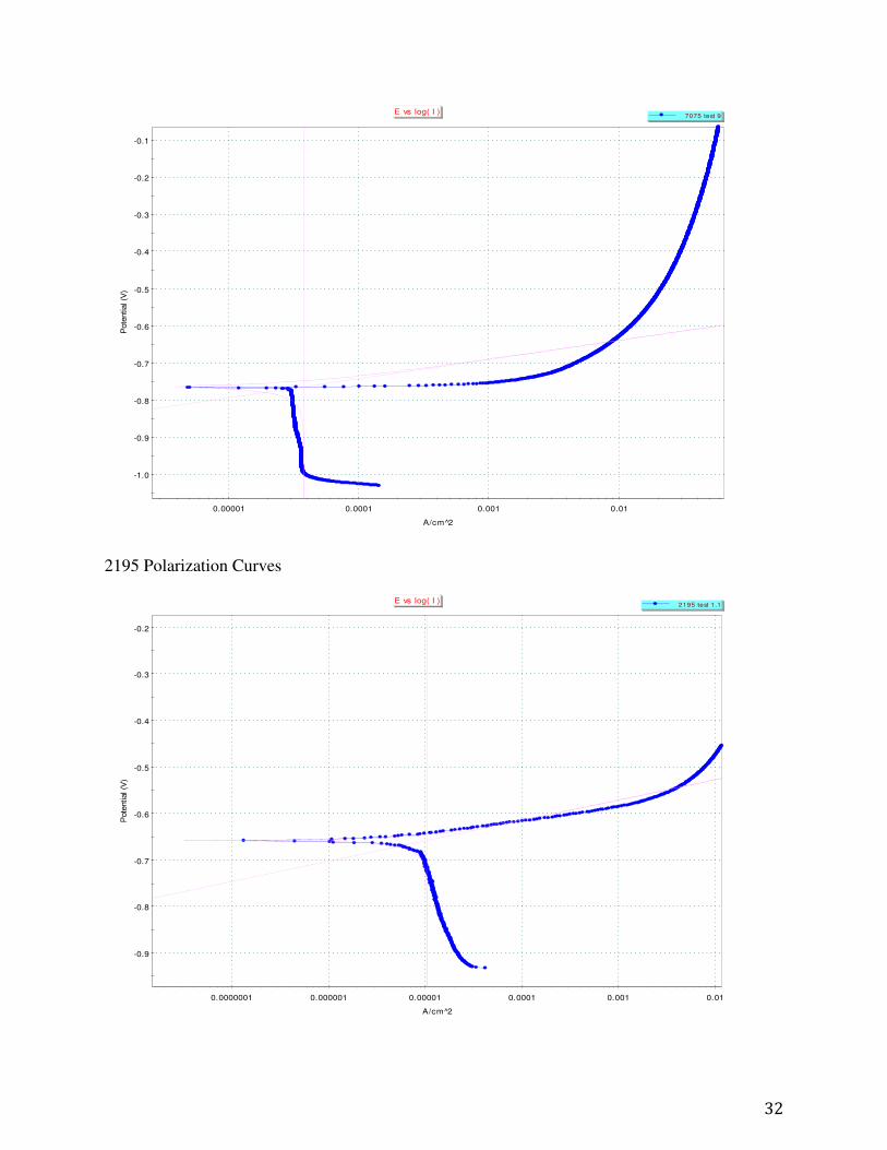
2195 Polarization Curves
-1.0
-0.9
-0.8
-0.7
-0.6
-0.5
-0.4
-0.3
-0.2
-0.1
0.00001 0.0001 0.001 0.01
Pote
ntial (V
)
A/cm^2
E vs log( I )7075 test 9
-0.9
-0.8
-0.7
-0.6
-0.5
-0.4
-0.3
-0.2
0.0000001 0.000001 0.00001 0.0001 0.001 0.01
Pote
ntial (V
)
A/cm^2
E vs log( I )2195 test 1.1

33
-0.9
-0.8
-0.7
-0.6
-0.5
0.0000001 0.000001 0.00001 0.0001 0.001
Pote
ntial (V
)
A/cm^2
E vs log( I )2195 test 2
-1.0
-0.9
-0.8
-0.7
-0.6
-0.5
-0.4
-0.3
-0.2
-0.1
0.0
0.1
0.2
0.00000001 0.000001 0.0001 0.01
Pote
ntial (V
)
A/cm^2
E vs log( I )2195 test 3

34
-0.72
-0.70
-0.68
-0.66
-0.64
-0.62
-0.60
-0.58
-0.56
-0.54
-0.52
0.000001 0.00001 0.0001 0.001 0.01
Pote
ntial (V
)
A/cm^2
E vs log( I )2195 test 4
-0.70
-0.68
-0.66
-0.64
-0.62
-0.60
-0.58
-0.56
-0.54
-0.52
-0.50
-0.48
-0.46
0.0000001 0.000001 0.00001 0.0001 0.001 0.01
Pote
ntial (V
)
A/cm^2
E vs log( I )2195 Test 5

35
-0.70
-0.69
-0.68
-0.67
-0.66
-0.65
-0.64
-0.63
-0.62
-0.61
-0.60
-0.59
-0.58
-0.57
-0.56
-0.55
-0.54
-0.53
-0.52
-0.51
0.0000001 0.000001 0.00001 0.0001 0.001
Pote
ntial (V
)
A/cm^2
E vs log( I )2195 Test 6
-0.71
-0.70
-0.69
-0.68
-0.67
-0.66
-0.65
-0.64
-0.63
-0.62
-0.61
-0.60
-0.59
-0.58
-0.57
-0.56
0.00000001 0.0000001 0.000001 0.00001 0.0001 0.001
Pote
ntial (V
)
A/cm^2
E vs log( I )2195 T est 7
36
-0.64
-0.63
-0.62
-0.61
-0.60
-0.59
-0.58
-0.57
-0.56
-0.55
-0.54
-0.53
-0.52
0.0000001 0.000001 0.00001 0.0001 0.001
Pote
ntial (V
)
A/cm^2
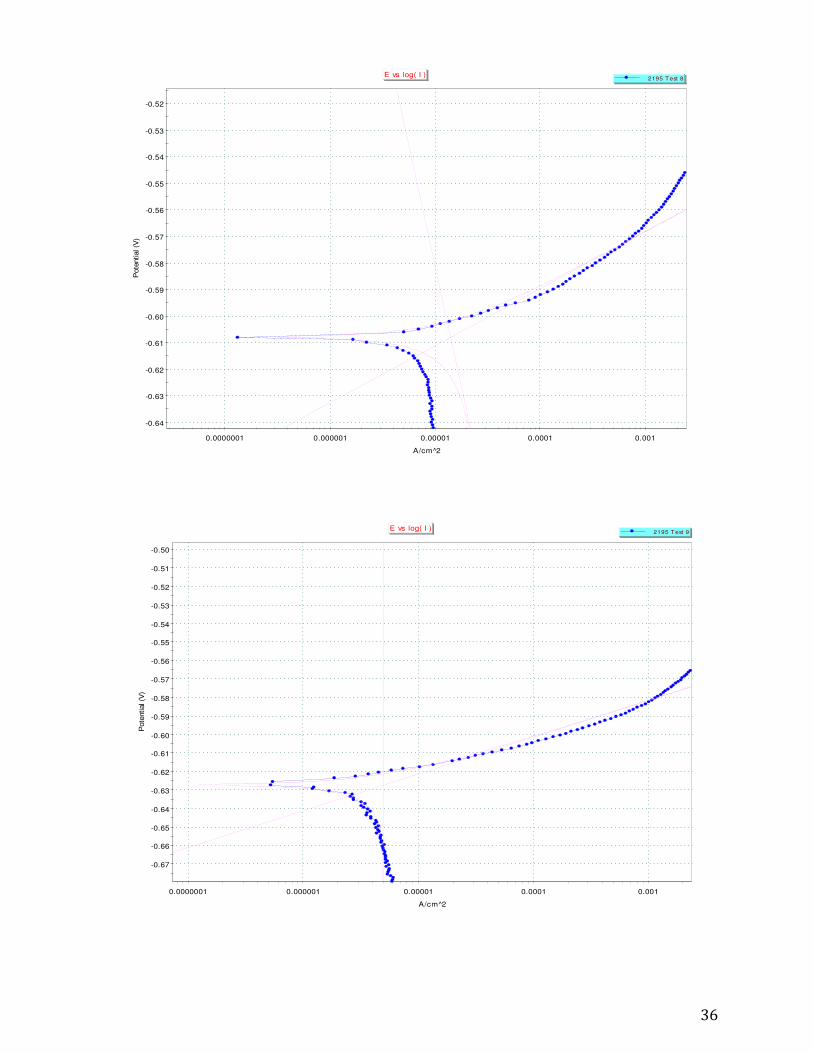
E vs log( I )2195 Test 8
-0.67
-0.66
-0.65
-0.64
-0.63
-0.62
-0.61
-0.60
-0.59
-0.58
-0.57
-0.56
-0.55
-0.54
-0.53
-0.52
-0.51
-0.50
0.0000001 0.000001 0.00001 0.0001 0.001
Pote
ntial (V
)
A/cm^2
E vs log( I )2195 Test 9

37
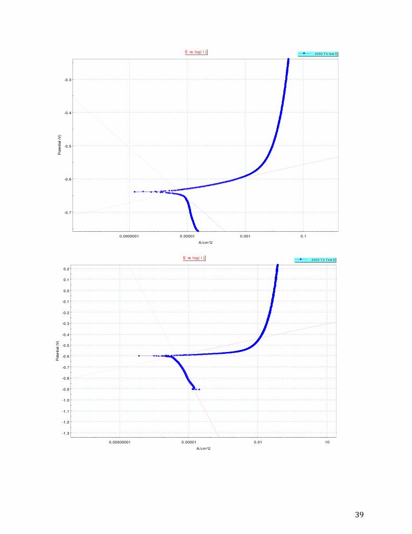
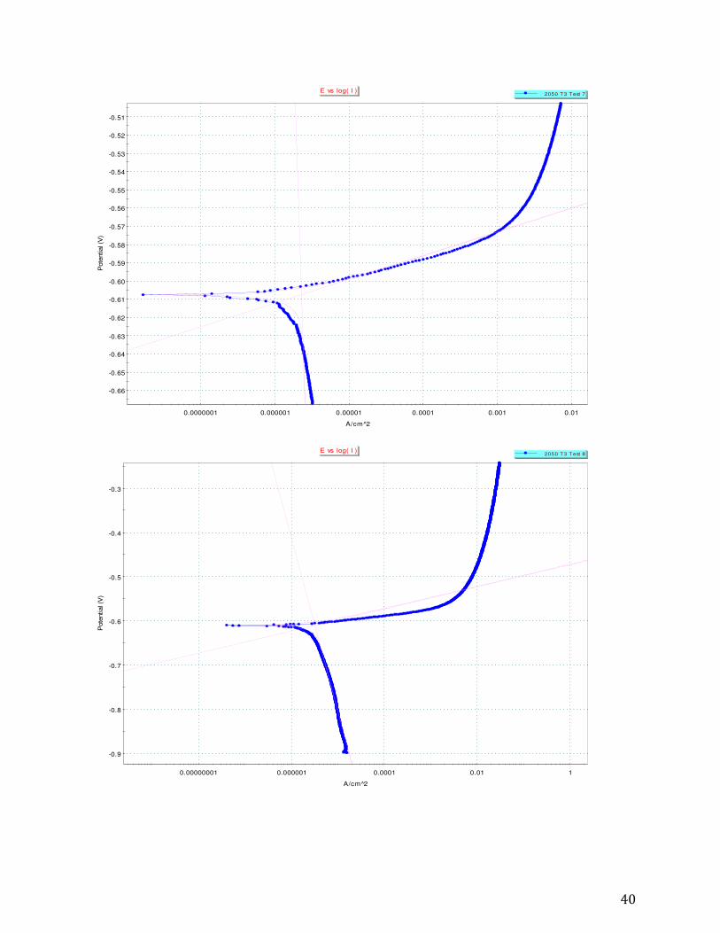
2050 T3 Polarization Curves
-0.72
-0.70
-0.68
-0.66
-0.64
-0.62
-0.60
-0.58
-0.56
-0.54
-0.52
-0.50
-0.48
0.0000001 0.00001 0.001 0.1
Pote
ntial (V
)
A/cm^2
E vs log( I )2050 T 3
-0.72
-0.70
-0.68
-0.66
-0.64
-0.62
-0.60
-0.58
-0.56
-0.54
-0.52
0.0000001 0.000001 0.00001 0.0001 0.001 0.01
Pote
ntial (V
)
A/cm^2
E vs log( I )2050 T3 test 2

38
-0.72
-0.70
-0.68
-0.66
-0.64
-0.62
-0.60
-0.58
-0.56
-0.54
-0.52
-0.50
-0.48
0.0000001 0.00001 0.001 0.1
Pote
ntial (V
)
A/cm^2
E vs log( I )2050 T3 test 3
-0.9
-0.8
-0.7
-0.6
-0.5
-0.4
-0.3
-0.2
0.00000001 0.000001 0.0001 0.01
Pote
ntial (V
)
A/cm^2
E vs log( I )2050 T3 test 4
39
-0.7
-0.6
-0.5
-0.4
-0.3
0.0000001 0.00001 0.001 0.1
Pote
ntial (V
)
A/cm^2
E vs log( I )2050 T3 test 5
-1.3
-1.2
-1.1
-1.0
-0.9
-0.8
-0.7
-0.6
-0.5
-0.4
-0.3
-0.2
-0.1
0.0
0.1
0.2
0.00000001 0.00001 0.01 10
Pote
ntial (V
)
A/cm^2
E vs log( I )2050 T3 Test 6
40
-0.66
-0.65
-0.64
-0.63
-0.62
-0.61
-0.60
-0.59
-0.58
-0.57
-0.56
-0.55
-0.54
-0.53
-0.52
-0.51
0.0000001 0.000001 0.00001 0.0001 0.001 0.01
Pote
ntial (V
)
A/cm^2
E vs log( I )2050 T3 Test 7
-0.9
-0.8
-0.7
-0.6
-0.5
-0.4
-0.3
0.00000001 0.000001 0.0001 0.01 1
Pote
ntial (V
)
A/cm^2
E vs log( I )2050 T3 Test 8

41
2050 T852 Polarization Curves
-0.70
-0.68
-0.66
-0.64
-0.62
-0.60
-0.58
-0.56
-0.54
-0.52
-0.50
0.0000001 0.000001 0.00001 0.0001 0.001 0.01
Pote
ntial (V
)
A/cm^2
E vs log( I )2050 T3 Test 9
-0.76
-0.74
-0.72
-0.70
-0.68
-0.66
-0.64
-0.62
-0.60
-0.58
-0.56
0.00000001 0.000001 0.0001 0.01
Pote
ntial (V
)
A/cm^2
E vs log( I )2050 T 852 test 1

42
-0.8
-0.7
-0.6
0.0000001 0.000001 0.00001 0.0001 0.001
Pote
ntial (V
)
A/cm^2
E vs log( I )2050 T852 Test 2
-0.72
-0.70
-0.68
-0.66
-0.64
-0.62
-0.60
-0.58
-0.56
-0.54
-0.52
-0.50
-0.48
0.0000001 0.00001 0.001 0.1
Pote
ntial (V
)
A/cm^2
E vs log( I )2050 T852 test 4

43
-0.9
-0.8
-0.7
-0.6
-0.5
-0.4
-0.3
-0.2
0.0000001 0.000001 0.00001 0.0001 0.001 0.01
Pote
ntial (V
)
A/cm^2
E vs log( I )2050 T852 Test 3
-0.66
-0.65
-0.64
-0.63
-0.62
-0.61
-0.60
-0.59
-0.58
-0.57
-0.56
0.000001 0.00001 0.0001 0.001
Pote
ntial (V
)
A/cm^2
E vs log( I )2050 T852 Test 5

44
-0.72
-0.70
-0.68
-0.66
-0.64
-0.62
-0.60
-0.58
-0.56
-0.54
-0.52
-0.50
-0.48
0.0000001 0.00001 0.001 0.1
Pote
ntial (V
)
A/cm^2
E vs log( I )2050 T852 Test 6
-0.72
-0.70
-0.68
-0.66
-0.64
-0.62
-0.60
-0.58
-0.56
-0.54
-0.52
0.0000001 0.000001 0.00001 0.0001 0.001 0.01
Pote
ntial (V
)
A/cm^2
E vs log( I )2050 T852 Test 7

45
-1.0
-0.9
-0.8
-0.7
-0.6
-0.5
-0.4
-0.3
0.0000001 0.00001 0.001
Pote
ntial (V
)
A/cm^2
E vs log( I )2050 T852 Test 8
-0.8
-0.7
-0.6
-0.5
0.0000001 0.00001 0.001 0.1
Pote
ntial (V
)
A/cm^2
E vs log( I )2050 T852 Test 9

46
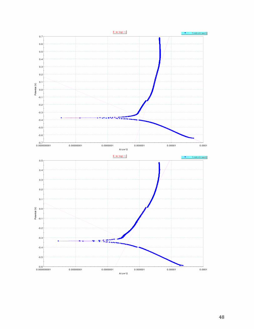
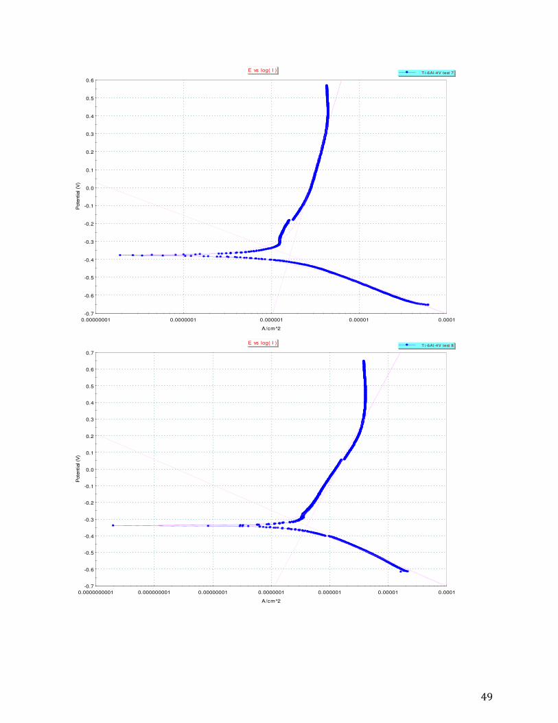
Ti-6Al-4V Polarization Curves
-0.7
-0.6
-0.5
-0.4
-0.3
-0.2
-0.1
0.0
0.1
0.2
0.3
0.4
0.000000001 0.00000001 0.0000001 0.000001 0.00001 0.0001
Pote
ntial (V
)
A/cm^2
E vs log( I )T i-6Al-4V test 1
-0.7
-0.6
-0.5
-0.4
-0.3
-0.2
-0.1
0.0
0.1
0.2
0.3
0.4
0.5
0.000000001 0.00000001 0.0000001 0.000001 0.00001 0.0001
Pote
ntial (V
)
A/cm^2
E vs log( I )T i-6Al-4V test 2

47
-0.7
-0.6
-0.5
-0.4
-0.3
-0.2
-0.1
0.0
0.1
0.2
0.3
0.4
0.000000001 0.0000001 0.00001
Pote
ntial (V
)
A/cm^2
E vs log( I )T i-6Al-4V test 3
-1
0
1
2
0.00000001 0.000001 0.0001
Pote
ntial (V
)
A/cm^2
E vs log( I )T i-6Al-4V test 4
48
-0.7
-0.6
-0.5
-0.4
-0.3
-0.2
-0.1
0.0
0.1
0.2
0.3
0.4
0.5
0.6
0.7
0.000000001 0.00000001 0.0000001 0.000001 0.00001 0.0001
Pote
ntial (V
)
A/cm^2
E vs log( I )T i-6Al-4V test 5
-0.6
-0.5
-0.4
-0.3
-0.2
-0.1
0.0
0.1
0.2
0.3
0.4
0.5
0.000000001 0.00000001 0.0000001 0.000001 0.00001 0.0001
Pote
ntial (V
)
A/cm^2
E vs log( I )T i-6Al-4V test 6
49
-0.7
-0.6
-0.5
-0.4
-0.3
-0.2
-0.1
0.0
0.1
0.2
0.3
0.4
0.5
0.6
0.00000001 0.0000001 0.000001 0.00001 0.0001
Pote
ntial (V
)
A/cm^2
E vs log( I )T i-6Al-4V test 7
-0.7
-0.6
-0.5
-0.4
-0.3
-0.2
-0.1
0.0
0.1
0.2
0.3
0.4
0.5
0.6
0.7
0.0000000001 0.000000001 0.00000001 0.0000001 0.000001 0.00001 0.0001
Pote
ntial (V
)
A/cm^2
E vs log( I )T i-6Al-4V test 8

50
-0.7
-0.6
-0.5
-0.4
-0.3
-0.2
-0.1
0.0
0.1
0.2
0.3
0.4
0.5
0.6
0.7
0.8
0.9
0.000000000001 0.0000000001 0.00000001 0.000001 0.0001
Pote
ntial (V
)
A/cm^2
E vs log( I )T i-6Al-4V test 9