Electroencephalogram Signals Classification by Ordered

Fuzzy Decision Tree

Jan Rabcan, Miroslav Kvassay

University of Zilina, Department of Infromatics, Univerzitna 8215/1,

010 26, Zilina, Slovakia

(jan.rabcan, miroslav.kvassay)@fri.uniza.sk

Abstract. A new algorithm for Electroencephalogram (EEG) signals classi-

fication is proposed in this paper. This classification is used for automatic de-

tection of patients with epilepsy in a medical system for decision support. The

classification algorithm is based on Ordered Fuzzy Decision Tree (OFDT) for

EEG signals. The application of OFDT requires special transformation of EEG

signal that is named as preliminary data transformation. This transformation ex-

tracts fundamental properties/features of EEG signals from every sample and

reduces dimension of the samples. The accuracy of the proposed algorithm was

evaluated and compared with other known algorithms used for EEG signal clas-

sification. This comparison showed that the algorithm proposed in this paper is

comparable with existing ones and can produce better results than others.

Keywords. Electroencephalogram, Classification, Ordered Fuzzy Decision

Tree

Key Terms. Model, Approach, Methodology, Scientific Field

1 Introduction

Epilepsy is characterized by the seizures that are the result of a transient and unex-

pected electrical disturbance of the brain. These electrical discharges of neurons are

evident in the electroencephalogram (EEG) signal, i.e. a signal that represents electri-

cal activity of the brain [1]. EEG has been the most common used signal for brain

state monitoring. It is used in medicine to reveal changes in the electrical activity of

the brain to detect disorders that are indicated generally at seizure diseases, loss of

consciousness after a stroke, inflammations, trauma, or concussion [2]. Measuring

brain electrical activity by EEG is considered as one of the most important tools in

neurology diagnostic [3, 4]. The specifics of this signal have been presented in details

in [3]. The communication in the brain cells takes place through electrical impulses.

EEG allows measuring these electrical impulses by placing the electrodes on the scalp

[1, 2]. Captured signals are amplified by EEG and then converted to the graphic rep-

resentation – curve [2]. The shape and character of the curves depend on the current

activity of the brain. By extracting useful information from captured signal, we are

able to predict or classify the brain state of investigated patient. However, the visual

inspection of EEG signal does not provide much information and, therefore, the au-

tomatic analysis and classification of EEG signal is a current problem. Solution to this

problem can permit developing decision support system for epilepsy diagnosis [1]–

[3]. By extracting useful information from the captured signal, the brain state of a

patient can be predicted or classified.

The specifics of EEG signal described in [1] imply special transformation of this

signal before application of classification procedure. This typical step of algorithms

for EEG classification is known as preliminary data transformation. The features ex-

traction and reduction of their dimension from the initial signal are fundamental pro-

cedures that are necessary before the classification. Different algorithms for features

extraction can be used for EEG signal, e.g. Fourier transform [4], logistic regression

[3], wavelet transform [2], Welch's method [4]. In this paper, we use Welch's meth-

od, whose result is a matrix of features that indicates specifics of the investigated

signal. However, this matrix has usually a large dimension for classification and,

therefore, a special procedure has to be used to reduce its dimension. The principal

component analysis (PCA) is used typically to achieve this goal in EEG signal analy-

sis. PCA is a statistical procedure [5, 19], which converts a set of observations (de-

scribed by variables that can be correlated) into a linearly uncorrelated smaller num-

ber of variables that are named as "principal components".

After the preliminary data transformation, the EEG signal can be classified. The

classification is implemented based on such methods as neural networks [4], evalua-

tion methods [5], clustering analysis [12], K-nearest neighbor classifier [6]. In [7],

decision tree has been used for EEG signal classification. The decision tree in [7] has

been inducted for numerical data. This required transformation of original EEG signal

into reduced data that can have some ambiguity [5], [8]. This ambiguity can be in-

cluded and considered in the analysis of data for the classification by their transfor-

mation into fuzzy data [9]. Fuzzy sets, which defines domains of fuzzy data, can be

useful to describe real-world problems with higher accuracy [10], [11]. This idea is

considered in this paper. We added one more step into the preliminary data transfor-

mation. In this step, the crisp data obtained after application of PCA is transformed

into fuzzy data in the process known as fuzzification.

In this paper, a new algorithm for classification of EEG signal that is transformed

into fuzzy reduced features is developed. The classification itself is implemented by

an Ordered Fuzzy Decision Tree (OFDT). This type of decision trees has been intro-

duced in [12], and its advantage is a regular structure that contains exactly one attrib-

ute at each level [11]. This implies the analysis based on this type of tree can be done

in a parallel way. In this paper, the OFDT for EEG signal classification is inducted

based on the data from source [13]. The accuracy of the classification was evaluated

and compared with other algorithms used for EEG signal classification.

This paper consists of four sections. The first section describes the background of

the proposed algorithm for EEG signals classification. This section describes data

used in the algorithm and explains the principal steps of the algorithm. The second

section deals with the preliminary data transformation by Welch’s method, principal

component analysis, and fuzzification. The process of OFDT induction is explained in

the third section. This process is illustrated using the data obtained after the prelimi-

nary data transformation of data from [13]. The fourth section provides estimation and

analysis of the implemented algorithm.

2 Background of New Algorithm of EEG Signal Classification

2.1 The Dataset Description

In case of epileptic activity, EEG signal has some special features that have to be

extracted automatically to allow classification. The development of new classification

algorithm requires application of data from real observations because they allow us to

evaluate the accuracy of the algorithm. The dataset of EEG signals used in this paper

was collected and published by R. G. Andrzejak in [13]. This dataset consists of five

subsets A, B, C, D and E, where each subset contains 100 samples. Every sample is

EEG segment of a patient of 23.6-sec duration. In subsets A and B, all samples were

taken from the surface of the head from five healthy persons. The difference of these

subsets is that the persons in subset A had eyes open while the persons in subset B

had eyes closed during EEG recording. According to [13], open or closed eyes of

patients have the influence on epileptic activity. Samples in subset D were recorded

from within the epileptogenic zone identified in the hippocampal formation, and those

in subset C were obtained from the hippocampal formation of the opposite hemi-

sphere of the brain. While subsets C and D contain only activity measured during

seizure-free intervals, subset E contains only seizure activity. All EEG signals were

recorded by the same 128-chanels amplifier system. After 12 bit analog-to-digital

conversion, the data were written continuously onto the disk of data acquisition com-

puter system at a sampling rate of 173.61 Hz. Band-pass filter setting was 0.53-40 Hz.

Examples of EEG signals from every subset are shown in Fig. 1.

The visual inspection of EEG signals depicted in Fig.1 does not provide much in-

formation. Also, the classification of these signals by decision tree, OFDT in particu-

lar, is not possible because these signals cannot be interpreted in terms of OFDT at-

tributes. This implies that some numerical features from these signals have to be ex-

tracted. Furthermore, if there are a lot of extracted features, then they should be re-

duced before the classification. This transformation of EEG signal is interpreted as

preliminary data transformation.

Fig. 1. Randomly chosen raw signals from each subset from [13]

2.2 Principal Steps of New Algorithm for EEG Classification by Ordered

Fuzzy Decision Tree

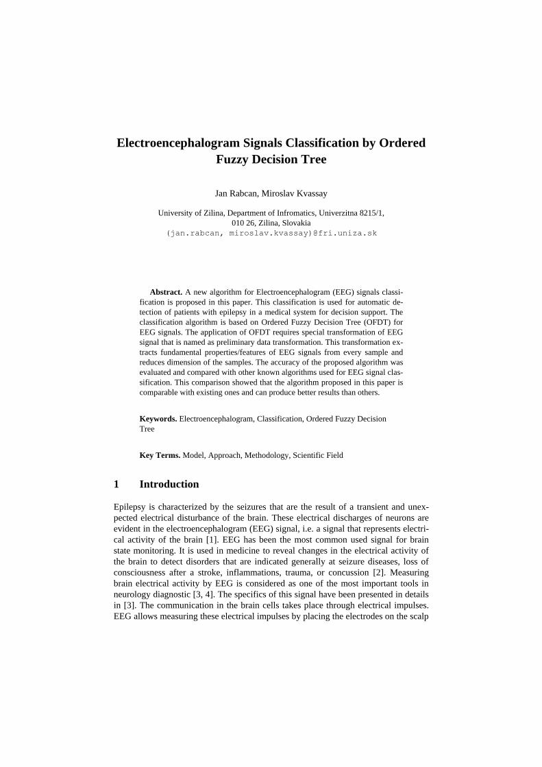
The new algorithm for EEG signal classification has 2 principal steps (Fig. 2): prelim-

inary data transformation and classification based on OFDT. The first of these steps

consists of three procedures. The first of them is feature extraction. There are different

procedures for extraction of features of EEG signal. For example, Fourier Transform

is used in [4], and wavelet transform in [2, 12]. In this paper, features have been ex-

tracted by Welch’s method, which represents one of the commonly used power spec-

tral density estimators.

The second procedure of the preliminary data transformation is a reduction of the

dimension. This procedure can be implemented based on the PCA, whose background

and principals are discussed in [19].

Finally, the third procedure is fuzzification of the obtained features of EEG signal.

This procedure is specific for our algorithm (it is not used in the existing ones), and its

addition results from application of classification algorithm based on OFDT. Several

algorithms can be implemented for this task. In this paper, we use algorithm of fuzzi-

fication that was described in [14].

The second step of the developed algorithm is classification. A new classification

based on OFDT is elaborated in this paper. The OFDT for this classification is induct-

ed based on estimation of cumulative information introduced in [15].

Fig. 2. The diagram of stages

3 Preliminary data transformation

3.1 Welch’s Method

The preliminary data transformation includes three procedures. The first of them is

Welch’s method that is used for extraction of the features from raw EEG segments.

The Welch’s method provides conversion from the time domain of the analyzed sig-

nal into its frequency domain. It is non-parametric power signal density estimator [4].

This transformation divides the time series of a signal into several overlapping seg-

ments of the same length, and then computes the periodogram of the each segment. The result of the Welch’s transformation is a matrix of features where every row cor-

responds with the periodogram of one signal. Every column is considered as input

attribute. As a rule, the obtained matrix has usually a lot of columns, i.e. a lot of input

attributes for the classification. To reduce the amount of input attributes PCA can be

applied.

3.2 Principal Component Analysis

PCA is a statistical procedure, which converts a set of observations (possibly correlat-

ed variables) into linearly uncorrelated variables called "principal components". The

number of principal components is less than or equal to the number of original varia-

bles. Every resulting principal component can be considered as an input attribute for

arbitrary classification model. The goal of the PCA is to maximize the variance of

individual principal components, provided that their covariance is equal to zero. The

resulting principal components are linear combinations of original features. In the

feature space, the components are orthogonal to each other. The first component has

the biggest variance. Every next component has as big variance as possible keeping

constraints that it is uncorrelated and orthogonal to the components obtained before

and its variance is bigger than variance of components after them. The number of

selected components for next analysis has been estimated by Kaiser’s criterion [16].

According to this criterion, a principal component is significant if its variance is

greater than the average variance of all the principal components. In some literature,

the result of PCA is denoted as an uncorrelated vector called orthogonal basis set [16].

3.3 Fuzzy Sets and Fuzzification

Input data for OFDT induction is fuzzy. This implies the numerical data obtained

from PCA has to be fuzzified. The fuzzification is the transformation of continuous

numerical data into a set of fuzzy data. One of the possible algorithms of fuzzification

is arbitrary clustering algorithm described in [16]. If data are fuzzified correctly, the

ambiguity of the original data can be reduced. Also, classification algorithm should be

less sensitive to errors and variations of measurements of EEG signals and, therefore,

it can result in obtaining better results of the classification process.

The classification algorithm considered in this paper works with fuzzy attributes.

Let us assume that we have 𝑛 fuzzy attributes denote as 𝐴𝑖, for 𝑖 = 1,2, … , 𝑛. Then

fuzzy attribute 𝐴𝑖 is a linguistic attribute, which means that 𝐴𝑖 can take fuzzy

ues 𝐴𝑖,𝑡 , 𝑡 = 1,2 … , 𝑄𝐴𝑖. Every value 𝐴𝑖,𝑡 of fuzzy attribute 𝐴𝑖 can be considered as a

fuzzy set. Fuzzy set 𝐴𝑖,𝑡 is defined as an ordered set of pairs {(𝑢, 𝜇𝐴𝑖,𝑡(𝑢)) , 𝑢 ∈ 𝑈},

where 𝑈 denotes the set containing all the entities belonged to the discourse (this set

is known as the universe of discourse or the domain of discourse), and 𝜇𝐴𝑖,𝑡(𝑢): 𝑈 →

[0,1] is a membership function that defines for every entity 𝑢 from universe U its

degree of membership to set 𝐴𝑖,𝑡 (a numeric value between 0 and 1). The membership

of entity 𝑢 from universe 𝑈 to fuzzy set 𝐴𝑖,𝑡 is defined by function 𝜇𝐴𝑖,𝑡(𝑢) in the

following manner:

1. 𝜇𝐴𝑖,𝑡(𝑢) = 0 if and only if 𝑢 is not a member of set 𝐴𝑖,𝑡 ,

2. 0 < 𝜇𝐴𝑖,𝑡(𝑢) < 1 if and only if 𝑢 is not a full member of set 𝐴𝑖,𝑡 ,

3. 𝜇𝐴𝑖,𝑡(𝑢) = 1 if and only if 𝑢 is a full member of set 𝐴𝑖,𝑡 .

In what follows, we will use some special terms from fuzzy set theory. The first of

them is cardinality 𝑀(𝐴𝑖,𝑡) of fuzzy set 𝐴𝑖,𝑡, which is defined as follows:

𝑀(𝐴𝑖,𝑡) = ∑ 𝐴𝑖,𝑡(𝑢)

𝑢∈𝑈

,

and another one is the product of fuzzy sets 𝐴𝑖,�̃� = 𝐴𝑖,1 × 𝐴𝑖,2 × … × 𝐴𝑖,𝑡. This product

results in new fuzzy set 𝐴𝑖,�̃�, which is defined as follows:

𝐴𝑖,�̃� = {(𝑢, 𝜇𝐴𝑖,1(𝑢) ∗ 𝜇𝐴𝑖,2

(𝑢) ∗ … ∗ 𝜇𝐴𝑖,𝑡(𝑢)) , 𝑢 ∈ 𝑈}.

The fuzzy attributes necessary for the OFDT induction in case of EEG signal clas-

sification have to be obtained by fuzzification of principal components obtained after

PCA transformation of data acquired by the Welch’s transformation of raw signals.

For this purpose, we use the arbitrary clustering algorithm. This algorithm divides

numerical values 𝑎 of the numerical attribute 𝑁𝑖 into 𝑄𝐴𝑖 clusters to obtain fuzzy at-

tribute 𝐴𝑖. The 𝑞-th cluster, for 𝑞 = 1,2, … , 𝑄𝐴𝑖, is described by center 𝐶𝑞. Creation of

membership functions is based on these centers. The usage of membership functions

𝜇𝐴𝑖,𝑞(𝑎) is explained in Table 1. The columns in Table 1 are separated into two sub-

columns. The first sub-column contains membership functions, and the second con-

tains obligations, which defines the function that will be used during the transfor-

mation.

Table 1. Table of membership functions

𝑢𝑖,1 𝑢𝑖,𝑞, for 𝑞 = 2,3, … , 𝑄𝐴𝑖− 1 𝑢𝑖,𝑄

𝜇𝐴𝑖,1(𝑎) If 𝜇𝐴𝑖,𝑞

(𝑎) If 𝜇𝐴𝑖,𝑄𝐴𝑖

(𝑎) If

1 𝑎 ≤ 𝐶1

0 𝑎 ≤ 𝐶𝑗−1

0 𝑎 ≤ 𝐶𝑄−1 𝑎 − 𝐶𝑗−1

𝐶𝑗 − 𝐶𝑗−1

𝐶𝑗−1 < 𝑎 ≤ 𝐶𝑗

𝐶2 − 𝑎

𝐶2 − 𝐶1

𝐶1 < 𝑎 < 𝐶2 𝐶𝑗+1 − 𝑎

𝐶𝑗+1 − 𝐶𝑗

𝐶𝑗 < 𝑎 ≤ 𝐶𝑗+1 𝑎 − 𝐶𝑄−1

𝐶𝑄 − 𝐶𝑄−1

𝐶𝑄−1 < 𝑎 ≤ 𝐶𝑄

0 𝑎 ≥ 𝐶2 0 𝑎 ≥ 𝐶𝑗+1 1 𝑎 ≥ 𝐶𝑄

The data for the OFDT induction is formed in the special table (Table 2). Every

sample of observations is represented by one output attribute B and n input

utes 𝐴𝑖, for 𝑖 = 1,2, … , 𝑛. The values of the output attribute represent class labels. The

repository table consists of 𝑛 + 1 columns that correlate with n input attributes and 1

output attribute B. Attribute 𝐴𝑖 is divided into 𝑄𝐴𝑖 sub-columns that correspond to the

values of the input attribute. The example of a repository is shown in Table 2. The

cells of this table contain the membership function values for every value of individu-

al attributes. A row in the table represents one sample used for OFDT induction.

Table 2. An example of the repository for OFDT induction

Input attributes, Ai Output attribute, B

A1 A2

. . .

An

A11 A1

2 A3

1

A21 A2

2 An

1 . . . An

QAn

B1 . . . B

QB

0.1 0.5 0.4 0.6 0.4 . . . 0.5 0.5 0.0 1.0

0.2 0.1 0.7 0.1 0.9 . . . 0.8 0.2 0.3 0.0

. . . . . . . . . . . . . . .

0.3 0.3 0.4 0.0 1.0 . . . 0.4 0.6 0.1 0.5

3.4 Results of Preliminary Data Transformation

The preliminary data transformation described above was applied on the data collect-

ed in [13]. Firstly, we used Welch’s method. This resulted in obtaining a matrix of

128 features (numeric attributes). After PCA application, the number of features was

reduced to 10 denoted as 𝐴1, 𝐴2, … , 𝐴10. Before their using in classification, we had to

fuzzify them. Their characteristics are presented in Table 3, whose second column

contains information about the percentage of the total variance contained in the indi-

vidual attributes (before fuzzification), and the third column presents the number of

fuzzy values for the individual attributes obtained after fuzzification.

Table 3. Characteristics of attributes obtained after preliminary data transformation

Attribute Variance after PCA in

percentage

Number of fuzzy values

after fuzzification

𝐴1 67.245 8

𝐴2 10.154 7

𝐴3 8.854 9

𝐴4 6.512 10

𝐴5 2.721 11

𝐴6 1.842 7

𝐴7 1.071 12

𝐴8 0.482 9

𝐴9 0.336 7

𝐴10 0.310 9

4 The Classification of EEG Signal by OFDT

4.1 OFDT Induction for EEG Signal Classification

According to [24], a decision tree is a formalism that allows recognition (classifica-

tion) of a new case based on known cases. Induction of a decision tree is a process of

moving from specific examples to general models and the goal of the induction is to

learn how to classify objects by analyzing a set of instances (already solved cases),

whose classes are known. Instances are typically represented as attribute-value vec-

tors. A decision tree consists of test nodes (internal nodes associated with input attrib-

utes) linked to two or more sub-trees and leafs or decision nodes labeled with a class

defining the decision. A test node is used to compute an outcome based on values of

the attributes of the instance, where each possible outcome is associated with one of

the sub-trees. Classification of the instance starts in the root node of the tree. If this

node is a test, the outcome for the instance is determined and the process continues

using the appropriate sub-tree. When a leaf is eventually encountered, its label gives

the predicted class of the instance. The OFDT is one of the possible types of decision

trees. It permits operating on fuzzy data (attributes) and term "ordered" means that all

nodes at the same level of the decision tree are associated with a same attribute [12].

The level of a node is defined by the number of nodes occurring on the path from the

root to the node.

Let us consider application of OFDT for classification of EEG signal that is repre-

sented by reduced features with fuzzy values. The splitting criterion for OFDT induc-

tion is the Cumulative Mutual Information (CMI) 𝐈(𝐵; 𝐴𝑖1, 𝐴𝑖2

, … , 𝐴𝑖𝑧−1, 𝐴𝑖𝑧

) [12],

[17], [18] where 𝐴𝑖1, 𝐴𝑖2

, … , 𝐴𝑖𝑧−1 is the sequence of nodes from the root to the inves-

tigated node and 𝑧 is the level of the investigated node. The attribute with the greatest

value of CMI is chosen to associate with all nodes at level z of the tree. The criterion

for choosing attribute that will be associated with level z of the tree can also take into

account the cost needed for obtaining value of attribute 𝐴𝑖𝑧. This characteristic of a

specific attribute is denoted as 𝐶𝑜𝑠𝑡(𝐴𝑖𝑧). The splitting criterion also tries to reduce

the number of branches in multi valued attributes. This can be achieved using the

entropy 𝐻(𝐴𝑖𝑧) of the investigated attribute. Therefore, the criterion for choosing the

attribute that will be used for splitting has the following form:

𝑞 = arg max (𝐈(𝐵; 𝐴𝑖1

, … , 𝐴𝑖𝑧−1, 𝐴𝑖𝑧

)

𝐻(𝐴𝑖𝑧) ∗ 𝐶𝑜𝑠𝑡(𝐴𝑖𝑧

)), (1)

where the entropy of attribute 𝐴𝑖𝑧is computed as 𝐻(𝐴𝑖𝑧

) = ∑ 𝑀(𝐴𝑖𝑧,𝑗𝑧) ∗

𝑄𝑖𝑗=1

(log2 𝑘 − log2 𝑀(𝐴𝑖𝑧,𝑗𝑧)), where 𝑘 is the count of data samples and z is the investi-

gated level of the OFDT.

The OFDT algorithm uses pruning technique for establishing leaf nodes. The goal

of pruning is to remove a part of an OFDT, which provides a small power for classifi-

cation of new instances. The used pruning method establishes the leaf nodes by stop-

ping the tree expansion during the induction phase. The pruning procedure uses the

threshold values 𝛼 and 𝛽. Threshold 𝛼 reflects the minimal frequency of occurrences

in a given branch. The frequency of a branch reflects percentage of instances belong-

ing to the given branch. (Please realize that one instance can belong to more than one

branch, which is caused by usage of fuzzy logic.) Threshold 𝛽 represents the maximal

confidence level computed in a given node. Confidence level means the likelihood of

the taken decision. Every internal node of the tree is declared as a leaf if at least one

of the following conditions is satisfied:

𝛼 ≥𝑀(𝐴𝑖1𝑗1

× … × 𝐴𝑖𝑧𝑗𝑧)

𝑘 (2)

𝛽 ≤ 2−𝐈(𝐵𝑗|𝐴𝑖1𝑗1,…,𝐴𝑖z𝑗𝑧) (3)

where 𝐴𝑖1𝑗1, … , 𝐴𝑖𝑧𝑗𝑧

is the sequence of specific values of attributes 𝐴𝑖1, … , 𝐴𝑖z

(this

sequence agrees with a path from the root 𝐴𝑖1 to node 𝐴𝑖z

), 𝐵𝑗 represents the j-th value

of output attribute B, where 𝑗 = 1,2, … , 𝑄𝐵, and 𝐈(𝐵𝑗|𝐴𝑖1𝑗1, … , 𝐴𝑖z𝑗𝑧

) is computed as:

𝑀(𝐴𝑖1𝑗1× … × 𝐴𝑖𝑧𝑗𝑧

) log2 𝑀(𝐴𝑖1𝑗1× … × 𝐴𝑖𝑧𝑗𝑧

× 𝐵𝑗)⁄ . These threshold values have

big influence on tree level and the depth of branches (paths from the root to a specific

node). The branch depth is defined as the number of nodes of given branch. Increas-

ing value 𝛽 causes increasing in the depth of tree branches. The parameter 𝛼 also

affects the depth of the tree. In this case, bigger 𝛼 causes the smaller depth of branch-

es. The threshold values should be set to good values to perform accurate classifica-

tion. If 𝛼 = 0 and 𝛽 = 1, the classification is very accurate, but only for training in-

stances. Small frequencies of branches will lead in classification mistakes of new

instances [19]. We use a simple method to determine the thresholds. The adjustment

of 𝛼 and 𝛽 values is performed by repeated induction of OFDT with different combi-

nations of the thresholds. After the heuristic finishes, the best combination is chosen.

The process is shown in Fig. 3.

Fig. 3. The diagram for estimation of thresholds 𝛼 and 𝛽

Modification of threshold values 𝛼 and 𝛽 allows induction of OFDT with accuracy

that agrees with problem conditions. OFDTs for different values of the threshold 𝛼

and 𝛽 can have different structure and accuracy.

4.2 Example of OFDT Induction

In the next part of this section, the induction of the OFDT will be illustrated. The

illustration is done for branch 𝐴1,1𝐴2,3. At the beginning of the OFDT induction, we

have set F of unused attributes. From set F we have to choose the attribute with max-

imal value of splitting criterion (1). We computed that the attribute with the maximal

value of the splitting criterion is 𝐴1. Therefore, this attribute is established as the root

of the tree. The frequency in the root calculated by (2) is always equal to 1. Attribute

𝐴1 has 2 fuzzy values 𝐴1,1 and 𝐴1,2. These values will be associated with outcomes

from the root. Attribute 𝐴1 is removed from set F of unused attributes. The first level

of the decision tree is displayed in Fig. 3.

Fig. 4. The first level of OFDT

At the second level, the attribute with a maximal value of (1) is selected from set F

again. In this case, attribute 𝐴2 has the maximal value of (1). This attribute is associ-

ated with the nodes at the second level of the tree. Next, it is necessary to check if

some node at the second level can be a leaf. The node is established as a leaf if at least

one of conditions (2) or (3) is satisfied. In explained branch 𝐴1,1𝐴2,3, branch 𝐴1,1, 𝐴2

has frequency equal to 0.543, which is greater than minimal frequency α, and confi-

dence levels are 0.547 and 0.453. This implies that condition (3) is also not satisfied

and, therefore, node 𝐴2 of branch 𝐴1,1, 𝐴2 cannot be a leaf.

Fig. 5. The second level of OFDT

At the third level, unused attribute 𝐴10 is chosen. This attribute is removed from set

F of unused attributes. At the third level two nodes become leafs. A leaf is established

in branch 𝐴1,1𝐴2,3, because condition (2) for minimal frequency is satisfied.

Fig. 6. The second level of OFDT

In a similar way the full OFDT displayed in Fig. 7 can be inducted. Every level of

this OFDT has exactly one attribute: the first level has one node with attribute A1, the

second level includes 2 nodes with attribute A2 and the third level has nodes agreeing

with attribute A10. The third level includes some nodes that are labeled as LEAF if the

node is a leaf. Every node has the information about the frequencies and confidence in

the second row and the last row accordantly. The confidence levels and frequencies

are calculated by formulas (2) and (3).

It can be unclear for someone why attribute A10 has been chosen at the 3-rd level of

the resulting OFDT since, after PCA transformation, the biggest amount of infor-

mation should be in first attributes while last attributes should have small amount of

information. This is caused by the splitting criterion because it takes into account the

output attribute too.

Please note we did not use fuzzification of the best quality in the illustration of

OFDT induction because we needed a tree of such sizes that can fit on the page (this

also affected on the sequence of chosen attributes). For the illustration purpose, we

also chose threshold 𝛼 for minimal frequency and threshold 𝛽 for maximal confidence

as 0.1 and 0.65 respectively. Therefore, the OFDT depicted in Fig. 7 does not agree

with one with the best reached accuracy.

Fig. 7. Final OFDT

5 Evaluation

5.1 Evaluation Procedure

The important characteristic of the classification procedure is the accuracy. The accu-

racy is estimated as the ratio between the count of correctly classified instances and

the number of classified instances, which represents the percentage of properly classi-

fied instances:

𝑎𝑐𝑐𝑢𝑟𝑎𝑐𝑦 = (∑ 𝑐(𝐼𝑖)

𝑘𝑖=1

𝑘) ∗ 100,

where 𝑘 is the number of classified instances, 𝐼𝑖 is the classified instance from dataset

𝐼, 𝑖 = 1,2, … , 𝑘 and 𝑐(𝐼𝑖) is given by:

𝑐(𝐼𝑖) = {1,0,

if 𝑐𝑙𝑎𝑠𝑠𝑖𝑓𝑦(𝐼𝑖) = class of 𝑥otherwise

,

where function classify returns the resulting class of OFDT classification.

The estimation of the accuracy of the classification can be done by two methods. In

first, the training and testing samples are the same. Each sample 𝐼𝑖 from dataset 𝐼 is

used to induct the OFDT. Then each sample 𝐼𝑖 ∈ 𝐼 is classified, and the accuracy is

evaluated. The second estimation is provided with the divided set of instances 𝐼. First-

ly, the set of instances 𝐼 is split into two sets. The first set contains training samples

and the second one testing samples. About 20% of samples of dataset 𝐼 are used for

classification (testing samples) and about 80% for OFDT induction (training sam-

ples). The described process is shown in the Fig. 8.

Fig. 8. Diagram of the accuracy estimation

5.2 Evaluation of Accuracy of Algorithm For EEG Signal Classification by

OFDT

The accuracy evaluation was implemented by several experiments. According to [7,

20, 21, 22, 23] evaluation of algorithms for EEG classification should be performed to

assess the accuracy of the samples division into two groups that agree with EEG of

healthy persons (subsets A and B) and sick persons (subsets C, D, E). Based on the

method presented in this paper, we implemented several classifications by OFDT

(Table 4). Every classification agreed with one experiment. The main difference be-

tween the experiments was the target of classification.

The goal of experiment 1 was to detect epileptic segments. Therefore, only two

output classes were needed: (AB) and (CDE). The first class represents healthy per-

sons and the second epileptics. The classification in experiment 2 estimated accuracy

for the division into 5 separate subsets (A, B, C, D, E) according to dataset description

in section 1.1. Experiment 3 focused on the seizure detection. This experiment repre-

sents also binary classification. One class represents segments with seizure activity

(E), while the second without the activity (ABCD). Experiment 4 aimed at estimation

of the subsets of the classified segments from the dataset. It was similar to experiment

2, but the subset with seizure activity (E) was not included. Experiment 5 was also

binary classification. The subset with seizure activity (E) was removed and the target

of the classification was to estimate healthy (AB) and epileptic (CD) segments.

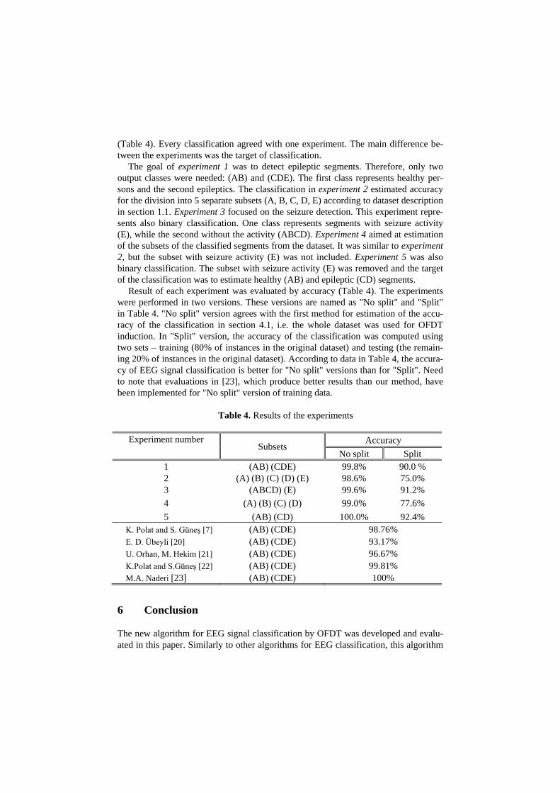
Result of each experiment was evaluated by accuracy (Table 4). The experiments

were performed in two versions. These versions are named as "No split" and "Split"

in Table 4. "No split" version agrees with the first method for estimation of the accu-

racy of the classification in section 4.1, i.e. the whole dataset was used for OFDT

induction. In "Split" version, the accuracy of the classification was computed using

two sets – training (80% of instances in the original dataset) and testing (the remain-

ing 20% of instances in the original dataset). According to data in Table 4, the accura-

cy of EEG signal classification is better for "No split" versions than for "Split". Need

to note that evaluations in [23], which produce better results than our method, have

been implemented for "No split" version of training data.

Table 4. Results of the experiments

Experiment number Subsets

Accuracy

No split Split

1 (AB) (CDE) 99.8% 90.0 %

2 (A) (B) (C) (D) (E) 98.6% 75.0%

3 (ABCD) (E) 99.6% 91.2%

4 (A) (B) (C) (D) 99.0% 77.6%

5 (AB) (CD) 100.0% 92.4%

K. Polat and S. Güneş [7] (AB) (CDE) 98.76%

E. D. Übeyli [20] (AB) (CDE) 93.17%

U. Orhan, M. Hekim [21] (AB) (CDE) 96.67%

K.Polat and S.Güneş [22] (AB) (CDE) 99.81%

M.A. Naderi [23] (AB) (CDE) 100%

6 Conclusion

The new algorithm for EEG signal classification by OFDT was developed and evalu-

ated in this paper. Similarly to other algorithms for EEG classification, this algorithm

includes two steps: preliminary data transformation and classification (Fig. 1). How-

ever, in the new algorithm, the additional procedure is included in preliminary data

transformation. This step performs fuzzification of reduced EEG signal features,

which permits taking into account the ambiguity of data for classification caused by

the initial EEG signal transformation (feature extraction and dimension reduction).

Due to fuzzification, special methods for fuzzy data analysis have to be used in classi-

fication of EEG signal. In this paper, we used OFDT. The accuracy of the classifica-

tion by OFDT was evaluated and compared with other algorithms for EEG classifica-

tion. The various combinations of the output labels (classes) were analyzed. The pro-

posed classification models reached satisfied results in comparison with other studies.

In future investigation, other methods for fuzzy data analysis and classification

should be used. Also, preliminary data transformation can be realized in many ways.

For example, feature extractor which takes into account the output attribute can be

used instead of PCA. The Welch’s method transforms signal from time domain to the

frequency domain, but methods that can analyze signals in both domain exist. Exam-

ple of such method is the wavelet transform. The important goal of this investigation

is to develop a classification of EEG signal with maximal accuracy that can be used in

medical decision support systems.

Acknowledgment

This work is partly supported by grants VEGA 1/0038/16 and VEGA 1/0354/17.

References

1. L. D. Iasemidis, “Epileptic seizure prediction and control,” Biomed. Eng. IEEE

Trans., vol. 50, no. 5, pp. 549–558, 2003.

2. M. H. Libenson, Practical approach to electroencephalography, vol. 48, no. 11.

2010.

3. A. Subasi and E. Erc, “Classification of EEG signals using neural network and

logistic regression,” Comput. Methods Programs Biomed., no. 78, p. 87—99,

2005.

4. H. R. Gupta and R. Mehra, “Power Spectrum Estimation using Welch Method

for various Window Techniques,” Int. J. Sci. Res. Eng. Technol., vol. 2, no. 6,

pp. 389–392, 2013.

5. A.T.Tzallas and I.Tsoulos, “Classification of EEG signals using feature creation

produced by grammatical evolution,” Proc. of the 24th Telecommunications Fo-

rum (TELFOR), pp. 411–414.

6. L. Guo, D. Rivero, J. Dorado, C. R. Munteanu, and A. Pazos, “Automatic fea-

ture extraction using genetic programming: An application to epileptic {EEG}

classification,” Expert Syst. Appl., vol. 38, no. 8, pp. 10425–10436, 2011.

7. K. Polat and S. Güneş, “A novel data reduction method: Distance based data

reduction and its application to classification of epileptiform EEG signals,”

Appl. Math. Comput., vol. 200, no. 1, pp. 10–27, 2008.

8. D. Ley, “Approximating process knowledge and process thinking: Acquiring

workflow data by domain experts,” Conf. Proc. - IEEE Int. Conf. Syst. Man Cy-

bern., pp. 3274–3279, 2011.

9. N. Gueorguieva and G. Georgiev, “Fuzzyfication of Principle Component Anal-

ysis for Data Dimensionalty Reduction,” 2016 IEEE Int. Conf. Fuzzy Syst., pp.

1818–1825, 2016.

10. J. Rabcan, “Ordered Fuzzy Decision Trees Induction based on Cumulative In-

formation Estimates and Its Application,” ICETA, p. 6, 2016.

11. J. Rabcan and M. Zhartybayeva, “Classification by ordered fuzzy decision tree,”

Cent. Eur. Res. J., vol. 2, no. 2, 2016.

12. V. Levashenko and E. Zaitseva, “Fuzzy Decision Trees in Medical Decision

Making Support System,” Computer Science and Information Systems. ” in 2012

Federated Conference on Computer Science and Information Systems, pp. 213–

219, 2012.

13. R. G. Andrzejak, K. Lehnertz, F. Mormann, C. Rieke, P. David, and C. E. Elger,

“Indications of nonlinear deterministic and finite-dimensional structures in time

series of brain electrical activity: dependence on recording region and brain

state.,” Phys. Rev. E. Stat. Nonlin. Soft Matter Phys., vol. 64, no. 6 Pt 1, p.

61907, 2001.

14. Y. Yuan and M. J. Shaw, “Induction of fuzzy decision trees,” Fuzzy Sets Syst.,

vol. 69, no. 2, pp. 125–139, 1995.

15. I. T. Jolliffe, Principal component analysis, 2nd ed. NY: Springer, 2002.

16. J. I. Maletic and A. Marcus, Data Mining and Knowledge Discovery Handbook.

2005.

17. V. G. Levashenko and E. N. Zaitseva, “Usage of New Information Estimations

for Induction of Fuzzy Decision Trees,” Lect. Notes Comput. Sci., vol. 2412, pp.

493–499, 2002.

18. V. Levashenko, E. Zaitseva, M. Kvassay, and Deserno, “Reliability Estimation

of Healthcare Systems using Fuzzy Decision Trees,” Ann. Comput. Sci. Inf.

Syst., vol. 8, pp. 331–340, 2016.

19. J. R. Quinlan, “Induction of Decision Trees,” Mach. Learn., vol. 1, no. 1, pp.

81–106, 1986.

20. E. D. Übeyli, “Wavelet/mixture of experts network structure for EEG signals

classification,” Expert Syst. Appl., vol. 34, no. 3, pp. 1954–1962, 2008.

21. U. Orhan, M. Hekim, and M. Ozer, “EEG signals classification using the K-

means clustering and a multilayer perceptron neural network model,” Expert

Syst. Appl., vol. 38, no. 10, pp. 13475–13481, 2011.

22. K. Polat and S. Güneş, “Artificial immune recognition system with fuzzy re-

source allocation mechanism classifier, principal component analysis and FFT

method based new hybrid automated identification system for classification of

EEG signals,” Expert Syst. Appl., vol. 34, no. 3, pp. 2039–2048, 2008.

23. M. A. Naderi, “Analysis and classification of EEG signals using spectral analy-

sis and recurrent neural networks,” Biomed. Eng. (NY)., no. 11, pp. 3–4, 2010.

24. L. Rokach and O. Maimon, “Data Mining with Decision Trees. Theory and Ap-

plications.,” Qual. Assur., 2008.