electromagnetic compatibility for device design and system

Electromagnetic Compatibility for Device Designand System Integration

Karl-Heinz Gonschorek · Ralf Vick

ElectromagneticCompatibility for DeviceDesign and SystemIntegration

123

ISBN 978-3-642-03289-9 e-ISBN 978-3-642-03290-5DOI 10.1007/978-3-642-03290-5Springer Heidelberg Dordrecht London New York

Library of Congress Control Number: 2009934598

c© Springer-Verlag Berlin Heidelberg 2009This work is subject to copyright. All rights are reserved, whether the whole or part of the material isconcerned, specifically the rights of translation, reprinting, reuse of illustrations, recitation, broadcasting,reproduction on microfilm or in any other way, and storage in data banks. Duplication of this publicationor parts thereof is permitted only under the provisions of the German Copyright Law of September 9,1965, in its current version, and permission for use must always be obtained from Springer. Violationsare liable to prosecution under the German Copyright Law.The use of general descriptive names, registered names, trademarks, etc. in this publication does notimply, even in the absence of a specific statement, that such names are exempt from the relevant protectivelaws and regulations and therefore free for general use.

Cover design: eStudio Calamar S.L.

Printed on acid-free paper

Springer is part of Springer Science+Business Media (www.springer.com)

Prof. Dr.-Ing. Karl-Heinz GonschorekEMV-Beratung - EMC-ConsultantGostritzer Straße 10601217 [email protected]

Prof. Dr.-Ing. Ralf VickLehrstuhl fur ElektromagnetischeVertraglichkeitOtto-von-Guericke-UniversitatMagdeburgInstitut fur Grundlagen derElektrotechnik undElektromagnetische VertraglichkeitPostfach 412039016 [email protected]

Contents

1 Motivation and Overview ................................................................1 1.1 Availability of programs, mentioned in the book....................6 1.2 Availability of the figures, given in the book..........................6

2 Thinking in Voltages, Currents, Fields and Impedances ..............7

3 Electric Fields..................................................................................19 3.1 Effects of electric fields and their calculation .......................22

4 Magnetic Fields ...............................................................................29 4.1 Effects of magnetic fields......................................................29 4.2 Calculation of magnetic field strength of single and

multicore cables ....................................................................31 4.3 Magnetic fields of Geofol transformers ................................34 4.4 Magnetic stray fields of arbitrary arrangements of thin

wires ......................................................................................35 4.4.1 Magnetic field of a four conductor arrangement..........35 4.4.2 Magnetic fields of twisted cables.................................37 4.4.3 Example calculation with the program STRAYF ........39 4.4.4 Peculiarities of magnetic fields of twisted cables ........41

5 Electromagnetic Fields ...................................................................45 5.1 Characterization of Electromagnetic Waves .........................45 5.2 Effects of electromagnetic fields...........................................50 5.3 The elementary dipoles .........................................................54

5.3.1 Distance conversion .....................................................61 5.3.2 Field impedances .........................................................65

5.4 Effective height, effective antenna area, radiation resistance ...............................................................................68

5.5 Estimating the field strength of aperture antennas ................75 5.5.1 Power density and electric field strength in the far

field region ...................................................................76

5.5.2 Power density and electric field strength in the near field region ........................................................... 77

5.5.3 Description of the program APERTUR ....................... 79 5.5.4 Program SAFEDIST .................................................... 79

6 The Interference Model ................................................................. 83 6.1 Galvanic coupling ................................................................. 90

6.1.1 Measures against a galvanic coupling interference...... 92 6.2 Capacitive coupling............................................................... 93

6.2.1 Measures to lower the capacitive coupling .................. 95 6.3 Inductive coupling................................................................. 97

6.3.1 Magnetic decoupling.................................................. 100 6.3.2 Definition of an effective mutual inductance for a

multicore cable........................................................... 101 6.3.3 Measures to reduce the inductive coupling................ 104

6.4 Electromagnetic coupling.................................................... 106 6.4.1 Measures to reduce the electromagnetic coupling ..... 107 6.4.2 The λ/2-coupling model ............................................. 108 6.4.3 Some remarks regarding the estimation of the

electromagnetic coupling ........................................... 111

7 Intrasystem Measures .................................................................. 121 7.1 Some remarks regarding grounding, shielding, cabling,

and filtering ......................................................................... 123 7.1.1 Grounding .................................................................. 123 7.1.2 Shielding .................................................................... 124 7.1.3 Cabling....................................................................... 126 7.1.4 Filtering...................................................................... 129

7.2 Shielding against electric fields - shield of bars.................. 138 7.3 Shielding against magnetic fields........................................ 141

7.3.1 Shielding against static magnetic and very low frequency magnetic fields .......................................... 141

7.3.2 Shielding against medium frequency magnetic fields........................................................................... 149

7.3.3 Two parallel plates shielding against alternating magnetic fields ........................................................... 149

7.3.4 Hollow sphere shielding against magnetic fields....... 150 7.3.5 Hollow cylinder within a lateral magnetic field......... 151 7.3.6 Hollow cylinder within a longitudinal magnetic

field ............................................................................ 151 7.4 Shielding theory according to Schelkunoff – short and

concise................................................................................. 153

VI Contents

Contents VII

7.4.1 Source code of the program SHIELD ........................157 7.5 Leakages, openings, cavity resonances ...............................157

7.5.1 Leakages, signal penetrations ....................................159 7.5.2 Low frequency resonances, cavity resonances...........167

7.6 Cable coupling and cable transfer impedance.....................171 7.6.1 Cable coupling ...........................................................171 7.6.2 Coupling into untwisted and twisted two

conductor cables.........................................................173 7.6.3 Coupling into and between shielded cables ...............175 7.6.4 Cable shield connection at the device input...............200

8 Atmospheric Noise, Electromagnetic Environment and Limit Values ..................................................................................205 8.1 Atmospheric noise sources, electromagnetic

environment.........................................................................206 8.2 Conversion of limit values ..................................................218

8.2.1 Distance conversion ...................................................218 8.2.2 Conversion E H and H E ..................................220

9 EMC Engineering and Analysis ..................................................225 9.1 Development phases of a complex system..........................227

9.1.1 Conceptual phase .......................................................227 9.1.2 Definition phase .........................................................228 9.1.3 Construction and building phase................................230

9.2 EMC- Test planning ............................................................232 9.3 Execution of analysis ..........................................................242

10 Numerical Techniques for Field Calculation .............................247 10.1 Selecting the appropriate technique ....................................249 10.2 Plausibility check ................................................................256 10.3 Application examples of analysis........................................265

10.3.1 Investigation of resonances on a passenger car..........266 10.3.2 Influence of a dielectric material on the radiation

of a printed circuit board............................................267 10.3.3 Radiation of a mobile phone ......................................268 10.3.4 Electromagnetic field on a frigate ..............................269

10.4 Guidelines for using numerical methods.............................271 10.5 Application: Antenna coupling ...........................................275

10.5.1 General remarks to the N-port theory ........................275 10.5.2 Two port parameter....................................................276 10.5.3 Calculation of antenna coupling ................................278 10.5.4 Source code of the program MATCH........................283

VIII Contents

11 Model for Immunity Testing ....................................................... 285 11.1 Standardised immunity test methods................................... 286 11.2 Statistical approach to model the immunity ........................ 288

11.2.1 Malfunction probability ............................................. 289 11.3 Fault frequency function ..................................................... 292

11.3.1 Interpretation of the results of immunity tests ........... 295 11.4 Time variant immunity........................................................ 296

11.4.1 Modelling................................................................... 297 11.4.2 Immunity of microcontroller based equipment.......... 303

A1 Electric Fields of Rod Arrangements.......................................... 307 A1.1 Potential coefficients and partial capacitances.................... 308 A1.2 Horizontal conductors above ground .................................. 309

A1.2.1 Source code of the program HCOND........................ 315 A1.3 Vertical conductors above ground....................................... 315

A1.3.1 Source code of the program VROD........................... 320

A2 Magnetic Stray Fields................................................................... 321 A2.1 Stray field low installation of cables ................................... 321

A2.1.1 The single core cable (case (a) of chapter 4.2)........... 321 A2.1.2 Cable with one forward and one return conductor

(case (b) of chapter 4.2) ............................................. 322 A2.1.3 Use of two forward- and two return conductors

(case (c1) of chapter 4.2) ........................................... 323 A2.1.4 Installation of the forward and return conductors

above a common ground plane (case (c2) of chapter 4.2) ................................................................ 324

A2.1.5 Use of four forward and four return conductors (case (d) of chapter 4.2) ............................................. 325

A2.2 Computer program for predicting magnetic stray fields ..... 327 A2.2.1 Field of a finitely long wire ....................................... 327 A2.2.2 Field of a single layered coil ...................................... 329 A2.2.3 Considering phase relations ....................................... 333 A2.2.4 Source code of the program STRAYF....................... 335

A3 Self and Mutual Inductances ....................................................... 337 A3.1 Mutual inductance between a finitely long conductor on

the y-axis and a trapezoidal area in the xy-plane ................ 337 A3.2 Decomposition of an area in the xy-plane bounded by

straight lines ........................................................................ 340 A3.3 Treatment of arbitrary conductor loops in space................. 341

Contents IX

A3.4 Mutual inductance between 2 circular loops with lateral displacement........................................................................343

A3.5 Source code of the program MUTUAL ..............................345

A4 Elementary Dipoles ......................................................................347 A4.1 Hertzian dipole ....................................................................347

A4.1.1 Prediction of the field strength components for the general case ..........................................................347

A4.1.2 Solution for time harmonic excitation .......................349 A4.2 Current loop (loop antenna) ................................................353 A4.3 Comparison of the wave impedances..................................360

A5 The Polarization Ellipsis ..............................................................361 A5.1 Two dimensional case (Ez=0)..............................................362 A5.2 Three dimensional case – solution in the time domain .......364

A5.2.1 Some consideration regarding the plane of the polarization ellipse .....................................................367

A5.3 Three dimensional case – solution in the frequency range....................................................................................375

A6 Skin Effect and Shielding Theory of Schelkunoff......................377 A6.1 Skin effect of a conducting half space.................................377

A6.1.1 Strong skin effect within a cylindrical conductor ......379 A6.1.2 Weak skin effect within a cylindrical conductor........380

A6.2 Shielding theory according to Schelkunoff .........................380 A6.2.1 Introduction................................................................380 A6.2.2 Necessary equations...................................................381 A6.2.3 Shielding mechanism .................................................382 A6.2.4 Shielding efficiency ...................................................384 A6.2.5 Simple application of Schelkunoff’s theory...............384 A6.2.6 Procedure for a graphical determination of the

shielding efficiency ....................................................386 A6.2.7 Error estimations........................................................390 A6.2.8 Summary ....................................................................392

A7 Example of an EMC-Design Guide for Systems ........................393 A7.1 Grounding ...........................................................................393 A7.2 System filtering ...................................................................395 A7.3 Shielding .............................................................................395 A7.4 Cabling ................................................................................396

A8 25 EMC-Rules for the PCB-Layout and the Device Construction.................................................................................. 401

A9 Easy-to-use Procedure for Predicting the Cable Transfer Impedance ..................................................................................... 409 A9.1 Predicting the voltage ratio with help of an oscilloscope.... 413 A9.2 Predicting the voltage ratio by a network analyzer ............. 415

A10 Capacitances and Inductances of Common Interest ................. 421

A11 Reports of Electromagnetic Incompatibilities............................ 429

A12 Solutions to the Exercises............................................................. 435

A13 Physical Constants and Conversion Relations........................... 455 A13.1 Physical Units and Constants .............................................. 455 A13.2 Conversion table for pressure.............................................. 456 A13.3 Conversion table for energy ................................................ 457 A13.4 Conversion relations for electric and magnetic

quantities ............................................................................. 457 A13.5 Conversion of logarithmic quantities .................................. 458 A13.6 Abbreviations ...................................................................... 459

A14 Bibliography.................................................................................. 461

Index .............................................................................................. 467

X Contents

1 Motivation and Overview

After working for more than 30 years in the field of EMC; having pub-lished numerous papers on the subject of interference, counter measures and numerical field calculation; the idea emerged to collate all experi-ences, successful analysis techniques and solutions into one comprehen-sive book. This was done in 2003/04 and the book was published in 2005 in the German language. Discussions with colleagues and with the pub-lisher revealed that an English version of the book is desirable. Moreover, the discussions suggested, as expected, some areas for improvement. The two main areas of criticism were firstly, the inclusion of extensive program lists and secondly, the chapter regarding filtering.

Regarding the program lists, it was the original wish of the authors to have them printed. These have now been removed but remain available on the web-pages of the authors and in there place more application examples of the programs have been included. Only very small program lists have been left in.

It has been recognized that the chapter concerning filtering is more a concise theoretical treatment of Butterworth filters than a chapter describ-ing the necessary EMC-features. Therefore, this chapter has been ex-tended, showing more elements from the EMC-point of view and giving suggestions for an EMC-justified installation.

Considering the aforementioned arguments, this English version of the German EMC-book ‘EMV für Geräteentwickler und Systemintegratoren’ is not a simple translation, hopefully it is a further development. Neverthe-less more than 90% consists of translated German text.

Which young scientist has not experienced, that he published a paper or gave a presentation at a symposium, all the time being proud of his work. Then afterwards, seeking praise or criticism, learns that feedback is the ex-ception rather than the rule? But nevertheless, the next paper, the next in-vestigation or the next presentation is still prepared with great care and en-thusiasm.

So the idea to write this book rose from the idea to summarize the re-sults of the different publications and presentations; to compile and to show, as far as possible, the inner relations and dependences of the experi-

K.-H. Gonschorek, R. Vick, Electromagnetic Compatibility for Device Design and System Integration, DOI 10.1007/978-3-642-03290-5_1, © Springer-Verlag Berlin Heidelberg 2009

2 1 Motivation and Overview

ences gained in EMC-analysis, EMC-system planning, and defining coun-termeasures to overcome interference.

Shortly after starting it became clear that the degree of experience of a single human being is always limited. Therefore, in order to produce a comprehensive publication of EMC, a lot of problem solutions have to be taken from other papers and books and revised to fit into the foreseen con-cept. Moreover, the expert assessment of others has to be considered. For that reason at this point we must thank the experts of WATRI, Perth (Western Australian Telecommunication Research Institute), especially Dr. Schlagenhaufer, as well as Prof. Singer from the Hamburg University of Technology, who have generously contributed pictures, ideas and solu-tions without requesting acknowledgement or their source.

Starting with the idea to make the author’s own experiences the main topic of the book, it became immediately clear that the offered solutions have to be revised in order to make them accessible to engineers who are attempting to solve similar problems or who are searching for explanations to apparently unexplainable phenomena.

It is intended that this book is not an addition to the vast array of gener-ally excellent introductions to EMC. Rather it is envisaged that this book will give help and hints to the experienced engineer in the development and construction of electric and electronic products and systems. More-over it will provide help in planning new projects, help in solving actual interference cases, support in analysing apparent incompatibilities, but predominantly to find a way to assess the problem.

With this in mind, this book is intended to be an ‘EMC-assistant’ for engineers, in which strategies, ways and methods, diagrams, rules of thumb, background theory and computer tools are brought together, which are helpful in solving problems of electromagnetic incompatibilities.

Solving an interference problem by a means other than trial and error requires a deeper understanding of the physical background of the prob-lem. Therefore, this book tries, in annex chapters, to deliver the physical basis together with the necessary mathematics in order to provide a com-promise between completeness, necessity and precision. Reading the book you will find a lot of material familiar from your study of electromagnetic technique. An attentive observer will identify that the elementary dipoles play a special role in the physical picture presented by the authors. It may also be evident that the experiences of the authors are given predominantly at the system level, while for EMC-problems at the device and circuit board level valuable experience from other experts has been taken into ac-count.

1 Motivation and Overview 3

It is normally expected that EMC-books deliver solutions and if possible tailor-made solutions to specific problems the reader may have. This de-mand cannot be fulfilled by any book because the variety of incompatibili-ties is as vast as the electromagnetic technique and its applications. In con-trast an EMC-textbook is able to fulfil two requirements; firstly it may state and explain a certain number of basic measures, which are the basis for an interference free construction of a device or a system, regarding both susceptibility and emission. As an example we refer to grounding (measures to provide low potential differences also for high frequencies) where approximately 98% of all interference cases are related to bad or non problem-matched grounding. Secondly an EMC-textbook may ex-plain the physical interrelations and background in order to teach an under-standing of electromagnetic coupling phenomena. For instance, the way each voltage is associated with an electric field strength, each current with a magnetic one. For EMC, more than for other physical disciplines the say-ing is valid: “A known enemy is not a real enemy!” Converting this prov-erb to EMC, it could be said with great conviction: “If the source for the interference is known, better the reason for incompatibility has been de-tected, then the suppression and elimination of the interference is not the real big problem!”

Some available EMC-books suggest that knowing and using only a handful of equations and rules is sufficient for handling interference ques-tions, such installing an electromagnetic shield to eliminate radiation prob-lems or using a filter for conducted problems. Books which are easy to read and bring about the feeling of being an EMC-expert are generally of little value. They only serve as a first step to provide problem awareness and solutions, or better a solution methodology, may not be possible.

This EMC-textbook starts with the phenomenon: Currents, voltages and fields with their impedances are the electromagnetic quantities which carry wanted signals; these phenomenon as secondary effects may produce elec-tromagnetic incompatibilities. Whether a wanted signal of one circuit be-comes an interference signal for a second circuit is always a question of the power needed in both circuits for transporting the information.

For that reason after the second chapter, which is at the same time also an introduction into the EMC-thinking, the different field types will be highlighted. The usual classification of the electromagnetic technique into electric fields (chapter 3), magnetic fields (chapter 4) and electromagnetic fields is very suitable for treating the EMC. The propagation, the ability to produce (unwanted) signals, as well as the measures against interference depend strongly on the field type and its characteristics. Chapter 6 dis-cusses the interference model, in which the field couplings will be ex-


plored. Countermeasures, measures to lower the coupling will be described in chapter 7 (intrasystem measures).

A chapter about the actual situation in standardisation has been omitted consciously. However, standards and legal requirements are mentioned at their respective places as far as is necessary for explanation. Dramatic ac-cidents and damage caused by electromagnetic incompatibilities are often used in justifying the necessity of EMC-measures. It is no exaggeration, that 90 % of all EMC-work is associated with the fulfilment of legal re-quirements in terms of emission limits. The aim of chapter 8 is to intro-duce the philosophy of defining limit values. Starting with the natural noise sources, taking the requirements of licensed radio services into ac-count, the limit values for radiated emissions are discussed in more detail. In this area however, it seems only natural, that great differences exist be-tween civilian and military considerations.

In chapter 9 the sequence of steps is stated, which, especially for plan-ning the EMC of complex systems with antennas, has proven to be reason-able and economical. Converting this system planning methodology into a methodology to handle the development of new devices should prove a trivial task.

A special chapter (chapter 10) is dedicated to the simulation software for numerical analysis of electromagnetic fields and couplings. In this chapter the available programs with their mathematical background are briefly presented. This chapter is not meant to be an introduction to nu-merical field calculation in general; it is intended to provide help for the beginner in using modern simulation software and choosing the correct simulation method for analysis of their specific problem. The main focus of the chapter lays in the application. The chapter aims to show that the available programs are powerful tools, if they are used in the correct way. Hints are given for the economical implementation.

In order that the reader may become familiar with numerical field analy-sis some sample arrangements with reference solutions are given. These sample arrangements are chosen to have a certain practical relevance. A potential user of the described software can request the names and sources of commercial software packages from the authors. The user should take time to become familiar with the software by varying the parameters, but more than this, based on the given examples, he should gain confidence into the program he is going to use. A very powerful demo-version of the program package CONCEPT is kindly made available by Prof. Singer and Dr. Brüns. It can be downloaded from the web-site of the authors.

The discussion and significance of susceptibility tests and the expertise of one of the authors lead to the integration of a special chapter (chap-ter 11) handling such questions. The discussed items and related equations,

1 Motivation and Overview 5

based on the probability theory make it possible to state confidence inter-vals for the immunity of modern electronic circuits and devices against pulse shaped interference signals. In addition, the phenomenon of the time dependent susceptibilities is discussed.

Extensive derivations and diagrams are shifted into annex chapters. The annex furthermore contains an EMC-design guide for systems, which could be the basis for a project specific guideline of the reader.

Naturally a book is a self-presentation of the author(s) as given here. On the other hand this book should help to better analyse or solve one or an-other interference case whether artificial or real. In this case the goal of the book is achieved.

Starting with this English version of the book Prof. Vick is also stated as one of the main authors, hence he takes over the full responsibility for the contents, too.

Dresden, spring 2009 Karl H. Gonschorek Ralf Vick Remarks: In this text book the numbers are written as far as possible in

American notation; this means a decimal point is used instead of the usual German comma. Keep in mind in certain places it may not have been possible to change. Furthermore the frequency, the impedance, and also the electric quantities abbreviations are of-ten used in the German manner, for instance 1 GHz instead of 1 Gc.

Acknowledgement: A special thank has to be given to Mr. Mark Panitz from the University of Nottingham, Great Britain, who did a great job in polishing the English of this text.


1.1 Availability of programs, mentioned in the book

From the outset of German version of the book, it was planned to add a CD with the software mentioned within the text. This has been disregarded for a number of reasons, not at least for the short shelf life and the different operation systems of computers.

The program CONCEPT is, as stated earlier, made available as a very powerful demo-version by Prof. Singer und Dr. Brüns from the Hamburg University of Technology.

The other programs, which were produced by one of the authors during his professional life, are written in POWER-BASIC and in no way opti-mized. The information within the single chapters should be sufficiently comprehensive that an experienced user of modern computer resources should be able to create a respective program fully to his requirements and taste. In most cases he will quickly produce adequate results with demon-strative graphics via MATHEMATICA or a comparable program. It is also recognised that a hands-on engineer may wish to use a finished and reli-able program, without the need to learn programming or the use of math-ematic packages. In order to satisfy this demand the programs mentioned are available at the web-sites of the authors. Three options are offered:

1. source codes in POWER-BASIC, except for CONCEPT, or 2. executable elements of the programs, running under ‘WINDOWS’,

downloadable from the home page “http://www.ovgu.de/vick/emcbook.html“,

3. it is also possible to obtain source codes and the executables com-plete on a CD. In this case expenses of 12.-- Euro has to be paid in advance.

1.2 Availability of the figures, given in the book

Due to printing limitations all figures (diagrams, sketches, and pictures) in the book are reproduced in black and white. Should the reader desire col-our versions of diagrams and pictures these are available from the authors.

Thanks to the permission of the Springer publisher all figures of the book may be downloaded in TIF-format from the internet address “http://www.ovgu.de/vick/emcbook.html“. It is therefore possible for the reader of the book to obtain figures ready for education purposes or other-wise. The authors request that this book is cited as the source of the figure.

2 Thinking in Voltages, Currents, Fields and Impedances

In order to achieve the EMC of a device or system, several measures must be taken. These measures start by thinking about the layout of the circuit and the design of the printed circuit board. They comprise the support of the inner arrangement of components and the wiring of equipment and ex-tend up to the formulation of guidelines for the construction of the system. The measures include the application of grounding, filtering and shielding guidelines as well as the implementation of problem-matched wiring and cabling. Furthermore, they may comprise the planning of device placement and installation within a system. This variety of isolated and sometimes seemingly unrelated single measures can be brought together if one re-members some basic knowledge of electromagnetics:

• Electric charges produce electric fields. Electric fields on the other hand produce forces on other charges and these forces cause an un-bound charge to move.

• Moving electric charges (currents) produce a magnetic field. Mag-netic fields on the other hand produce forces on other moving elec-tric charges (currents). Time varying fields, which are produced by time varying currents, produce forces on electric charges at rest. This effect is called induction, producing an induction voltage.

• Temporal and spatial variations of electric and magnetic fields are related to each other. Time varying fields propagate as electromag-netic waves.

These properties of electric charges have to be accepted as given. In or-der to eliminate some common interference there are, in general, only the following possibilities:

• Currents must be suppressed (providing the currents are not needed as signal currents).

• Currents must be damped in such way, that the effects on other sys-tems are negligible.


8 2 Thinking in Voltages, Currents, Fields and Impedances

• Additional currents have to be driven, producing fields which com-pensate the initial fields.

The last point has a special meaning within the set of EMC-measures because shielding efficiency, the influence of ground planes, as well as the effectiveness of cabling with low stray fields can be related back to this principle.

Voltage: The starting point of every electromagnetic consideration is the elementary charge. It has a measured value of e = -1.609·10-19 C. A single elementary charge is so small (radius of an electron = 3.4 10-21 m) that an accumulation of charges, let’s say 106 elementary charges, can still be con-sidered as a point charge Q. The mass of the elementary charge, or electron is 9.14·10-31 kg.

Between two point charges there exists a force given by the vector:

rer

QQF2

21

4πε= (2.1)

If the charges have alternate polarities the force between them is attrac-tive. On the other hand, the force between charges of equal polarity is re-pulsive. If one charge, for instance Q2, is defined as a test charge and the force given by Eq. (2.1) is divided by the magnitude of the test charge, a new quantity is derived, termed the electric field strength:

rer

QQFE

21

2 4πε== (2.2)

Electric field strength: The electric field strength is the force per unit charge on a stationary charge. If electric field strength is present forces act upon charges, which can lead to their displacement.

Separating two charges (unequal polarity) over a certain distance re-quires a force to be applied over that distance. In other words, a defined amount of energy is required. Upon releasing the charges, they will move to collide and the energy will be gained back again. Therefore, a displace-ment of a charge in the direction of the electric field vector leads to gain in energy. By relating the energy gain to the test charge one can obtain the potential. A potential difference (movement from position 1 to position 2) between two points in space is called voltage. Hence, the voltage is a measure of the working potential of a given field. This means with relation to the ElectroMagnetic Compatibility:

If a voltage source is connected between 2 electrodes, charges on these electrodes and also on uninvolved metallic structures are displaced until

2 Thinking in Voltages, Currents, Fields and Impedances 9

on each electrode and on each metallic part an equal potential is obtained (equipotential). This statement equates to asserting that ‘The tangential electric field strength on a metallic surface is equal to zero!’.

If the voltage varies (for this consideration we assume a sinusoidal variation) from positive to negative the charges have also to follow this change in polarity. On all electrodes and metallic structures in which a movement of charges occurs it is prescribed that a current is flowing. If the voltage alteration is very fast it is possible that the charges are not able to follow this variation (transition from static considerations for a slowly al-ternating field to a high frequency field variation).

In the area of EMC a limit for the transition from static or stationary considerations to high frequency behaviour has been defined:

l = λ/10 (structure extension = 1/10 of the wave length). (2.3)

If the structure to be investigated is smaller than 1/10 of the smallest wavelength to be considered (wavelength of the highest frequency in ques-tion) it is satisfactory to use static or stationary approaches and considera-tions. We take here a main board of a computer with dimensions 30 cm by 20 cm as an example, if we assume a clock frequency of 400 MHz then high frequency investigations have to be carried out.

Current: Each movement of a charge is called an electric current. If in one second 6.3 1018 electrons (charge carriers) are flowing through a wire (the cross section of the wire), then it is defined that the current will be 1 A. The single charge carriers take their polarity with them to attract or to push away other charge carriers. Additionally, there appears a second force effect acting on moving charges:

),( BxvqF = (2.4)

q = charge, which moves with the velocity v, B = magnetic flux density, for instance produced by another cur-

rent. The electric current in the first approach produces a magnetic field

strength, which can easily be converted for non-magnetic materials to a magnetic flux density using the B = μH – relation.

Furthermore, for simple arrangements the magnetic field strength may be calculated by the Ampére’s Law:

IsdH =∫ ⋅ . (2.5)

Here the critical feature is the fact that every current produces a mag-netic field, which in turn leads to a force on other moving charges. Only


full metal screens with a completely symmetrical construction do not have an electric or magnetic field in the surrounding space.

In order to transfer electric energy or information from one place to an-other by electromagnetic means, electric voltages or currents are required. Therefore, it would seem impossible (except in special cases like the fully symmetrical fully shielded coaxial cable) to avoid electric and magnetic fields. For that reason, the task of EMC can not be to eliminate the re-quired currents or voltages, but to provide defined places and paths for them so that the effects on other circuits can be kept sufficiently low.

For completeness at this point it should be mentioned that there are also convection currents that exist, which are detached from metallic conduc-tors. These are not normally a concern for the subject of EMC. Further-more, current loops may also be closed via displacement currents, where a displacement current is always produced when a time varying electric field occurs in a dielectric material.

Impedance: If the voltage of a circuit or a loop is divided by the produced current the input impedance at that point is obtained. The impedance con-sists of a real and an imaginary part. The real part describes the losses in the circuit; the imaginary part is a measure of the fields related to the volt-age and current in the circuit or loop. The imaginary part may be capaci-tive and becomes smaller with increasing frequency; or inductive and be-comes larger with increasing frequency.

The current will always use the path of lowest resistance. If we also consider complex impedances we can extend this theorem: The current al-ways uses the path of lowest impedance.

This simple theorem has a very special meaning in the area of EMC. If interference occurs and the interference source is known then the coupling path, or the route of the current, has to be found. Remembering that the current is using the path of lowest impedance reduces the task to finding this transfer route. In this analysis it has to be considered that, not only do discrete elements have to be taken into account, but that current loops can also close via electric or magnetic stray fields. Furthermore, these stray fields have effective impedances which have to be included in the analysis.

The following first example may serve as a demonstration of the behav-iour of the current: 10 cm above a conducting plane (with losses) a cylin-drical conductor (made from copper) of a total length of 1.2 m and a radius of 1 mm is installed. The conductor is arranged in such a way that it is bent at its half length by an angle of 90 degrees. It is required to calculate the surface current and equivalently the return current within the plane. The arrangement is given in Fig. 2.1. The driving voltage is located at the left end of the wire between the wire and ground plane, the generator has a


source impedance of 50 Ω. The right end of the wire is directly connected to the conducting plane.

Fig. 2.2 shows the surface current on the plane for the following fre-quencies: 1 kHz, 10 kHz, 100 kHz, and 1 MHz. It is very demonstrative to see that for a frequency of 1 kHz the direct path from the short circuited right end to the feeding point is taken. At this frequency this path has the lowest impedance. At 10 kHz it can be seen that the current is drawn slightly to the conductor and at 100 kHz the current is nearly completely following the path of the wire. It can be presumed, taking the self induc-tance into account, that every other path has a higher impedance.

Fig. 2.1 Arrangement of a bent conductor above a conducting plane

Fig. 2.2 Currents in the plane for a) 1 kHz, b) 10 kHz, c) 100 kHz, d) 1 MHz

-0,5,

-0,5,

0,0

-0,05,

-0,05,

0,1

-0,05,

0,55,

0,1

0,55,

-0,05,

0,1

1,0,

-0,5,

0,0

1,0,

1,0,

0,0

-0,5,

1,0,

0,0

a) b)

c) d)


1 mm 1 mm

d =

3.7

mm

240

0.001

I

I

I

U

0

R

M

0= 1 V

d = 0.2 m

l l

l

, ,

=

1 m

3.74 mm

2r = 2r =

2r =

ZL

ZL

ZL

MS

MS

MS

ZLR

ground loop

Fig. 2.3 Two conductor arrangement, in which the return conductor is connected

to ground forming a ground loop

With the second example, which can also be treated analytically, it is in-tended to clearly show the effect of field concentration. The arrangement (Fig. 2.3) consists of a 240 Ω two conductor arrangement, in which the re-turn wire is connected directly to ground at both ends, effectively forming a ground loop. The relative arrangement parameters have been chosen in such a way that the ground loop resistance is only 1/10 of the return wire resistance. By feeding the arrangement with a DC-voltage it is found that 91 % of the total current is flowing via the ground; only 9 % of the total current is to be found in the dedicated return conductor.

From the data stated above and a conductivity of κ = 57 106 S/m the fol-lowing network parameters can be calculated:

Resistance of the return wire:

mΩ3.222 =⋅

=R

RR

rlR

κπ (2.6)


Resistance of the ground loop:

mΩ23.22 =⋅

=M

MM

rlR

κπ (2.7)

Inductance per m of the two conductor line:

μH/m8.0ln' =⋅≈ZLZL

ZL rdL

πμ (2.8)

Capacitance per m of the two conductor line:

pF/m9.13ln

' =≈

ZLZL

ZL

rdC επ

(2.9)

Self inductance of the ground loop:

μH13.2ln =⋅

⋅⋅

≈MSZL

MSMSMS rr

dlLπ

μ (2.10)

Mutual inductance between the two conductor circuit and ground loop:

μH4.02

ln2

'=

⋅≈⋅

⋅≈ ZWZL

ZLZLZW lL

rdlM

πμ (2.11)

Remark: For LMS and M the simplified formulas of parallel conductors have been used.

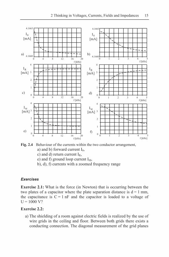
In Fig. 2.4 the currents I0, IR und IM as function of frequency are plotted, as they have been obtained using the program CONCEPT. Subfigures a), c) and e) show the frequency range 100 Hz to 20 kHz and the remaining subfigures b), d), f) show the range 100 Hz to 5 kHz.

Examining the behaviour of the currents IM and IR of Fig. 2.4 as function of frequency the following results can be recognized:

1. At the frequency 0 Hz (here for the calculation at 100 Hz) the return current is divided in accordance with the associated resistances. 91 % of the return current is flowing in the ground loop and only 9 % is flowing in the dedicated return conductor.

2. With increasing frequency the inductive part of ground loop imped-ance becomes greater and greater. At a frequency of f3dB = 1.7 kHz it reaches a value equal to the return wire resistance ωLMS = RR (The skin effect does not need to be considered at this frequency). A sig-


nificant proportion of the return current is now flowing via the dedi-cated return conductor.

3. With further increasing frequency the inductive reactance of the ground loop becomes higher and higher. The result is that the total re-turn current is now flowing via the dedicated return conductor. How-ever, due to the mutual inductance M between the two conductor cir-cuit and the ground loop, a current in the ground loop will occur. The effect of this is that the measurable return current will be reduced to

⎟⎟⎠

⎞⎜⎜⎝

⎛−⋅≈

MSR L

MII 10 . (2.12)

In the ground loop a current of MS

MS LMII ⋅≈ 0 is flowing.

Taking I0 = 1 V/240 Ω = 4.2 mA and M/LMS = 0.19 results in a measur-able current in the dedicated return wire of IR = 3.4 mA; this result is in very good agreement with the simulation results. In the ground loop a cur-rent of 0.8 mA (for this particular arrangement) is still flowing; it is this current which is the main contributor to the radiation.

It is proposed that a reduction in the ground loop current is required. To do this the mutual inductance M between the two conductor arrangement and the ground loop has to be reduced; in the ideal case it should reduced to zero. This can be achieved by twisting the two conductor line or by us-ing a coaxial cable for the information channel. With respect to the self in-ductance of the ground loop the degree of freedom is very limited. To in-crease the self inductance of the ground loop would mean making the loop size greater, a solution which is contradictory to the requirement of mini-mizing the loop to limit coupling and radiation.


Fig. 2.4 Behaviour of the currents within the two conductor arrangement,

a) and b) forward current I0, c) and d) return current IR, e) and f) ground loop current IM, b), d), f) currents with a zoomed frequency range

Exercises

Exercise 2.1: What is the force (in Newton) that is occurring between the two plates of a capacitor where the plate separation distance is d = 1 mm, the capacitance is C = 1 nF and the capacitor is loaded to a voltage of U = 1000 V?

Exercise 2.2:

a) The shielding of a room against electric fields is realized by the use of wire grids in the ceiling and floor. Between both grids there exists a conducting connection. The diagonal measurement of the grid planes


in the ceiling and floor is D = 10 m, the distance between ceiling and floor is measured to d = 3 m. Up to what frequency is it acceptable to use static field considerations to approximate the shielding effi-ciency?

b) The main board of modern personal computers have dimensions of 30 cm × 20 cm. Up to what frequency might it be acceptable to accu-rately calculate the internal couplings and unwanted interactions on the board by static and stationary field assumptions?

Exercise 2.3: A very long metal plate of a width of b = 10 cm is guiding a current of I = 10 A. How big is the magnetic field strength at a distance of d = 1 cm:

a) away from the edge of the plate,

b) above the middle of the metal plate?

Exercise 2.4: An electron is moving with a speed of vx = 60 000 km/s through a magnetic field of Hz = 2 A/m. How large is the deflection d, per-pendicular to the electron’s initial trajectory, after moving a distance of s = 30 cm?

Exercise 2.5: At a frequency of f = 50 Hz a twisted three conductor cable is producing, at a distance of rM = 10 cm from the cable axis, a magnetic flux density, which can be described by Bϕ = B0 cos (2 π x/SL); where SL = turn width = 0.8 m, B0 = 10 µT. The magnetic flux density is directed perpendicularly into an interference area. The interference area has a radial extension (with respect of the cable axis) of d = 1 cm (starting at r = 9.5 cm) and an axial extension of Δx, starting at x = 0.

a) After what length Δx of the area does the coupling (open circuit volt-age) reach its maximum?

b) How large is the maximum open circuit voltage?

c) After what length Δx of the area does the coupling reach its mini-mum?

Remark: The radial dependence of the field is neglected!

d) The area in which the induction may take place is surrounded by a closed copper wire of a thickness of 2R = 0.4 mm. How large is the current flowing in the influenced wire loop?

e) At what frequency is the resistance of the wire loop equal to the in-ductive reactance (RW = ωL)?


Remark: The self inductance of the influenced loop may be calculated using the relations of a two conductor arrangement.

3 Electric Fields

Electromagnetic fields are described mathematically by the four Max-well’s equations. Expressed in integral form they are:

Ampère’s circuital law

,L Vs A A

H ds J dA D dA I It

∂∂

⋅ = ⋅ + ⋅ = +∫ ∫ ∫ (3.1)

Gauss’ law

,A V

D dA dV Qρ⋅ = ⋅ =∫ ∫ (3.2)

Faraday’s law of induction

∂⋅ = − ⋅ = −

∂∫ ∫s A

E ds B dAt t

∂ φ∂

, (3.3)

0A

B dA⋅ =∫ , (3.4)

H = magnetic field strength, J = current density, D = displacement current density,

LI = conductor current, VI = displacement current,

ρ = charge density, Q = electric charge, E = electric field strength, B = magnetic flux density, φ = magnetic flux,

sd = infinitesimally small element of the contour of area A , Eqs. (3.1) and (3.3).


20 3 Electric Fields

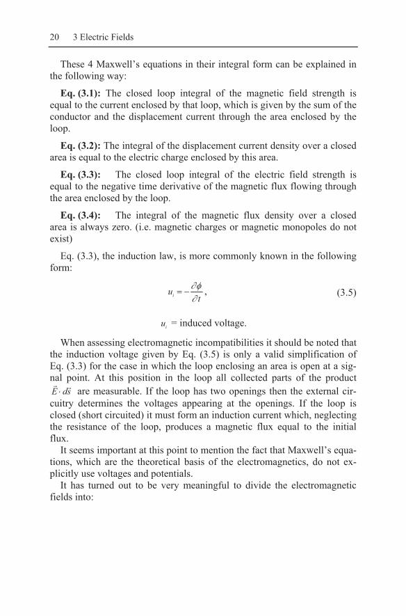
These 4 Maxwell’s equations in their integral form can be explained in the following way:

Eq. (3.1): The closed loop integral of the magnetic field strength is equal to the current enclosed by that loop, which is given by the sum of the conductor and the displacement current through the area enclosed by the loop.

Eq. (3.2): The integral of the displacement current density over a closed area is equal to the electric charge enclosed by this area.

Eq. (3.3): The closed loop integral of the electric field strength is equal to the negative time derivative of the magnetic flux flowing through the area enclosed by the loop.

Eq. (3.4): The integral of the magnetic flux density over a closed area is always zero. (i.e. magnetic charges or magnetic monopoles do not exist)

Eq. (3.3), the induction law, is more commonly known in the following form:

tui ∂

φ∂−= , (3.5)

iu = induced voltage.

When assessing electromagnetic incompatibilities it should be noted that the induction voltage given by Eq. (3.5) is only a valid simplification of Eq. (3.3) for the case in which the loop enclosing an area is open at a sig-nal point. At this position in the loop all collected parts of the product

sdE ⋅ are measurable. If the loop has two openings then the external cir-cuitry determines the voltages appearing at the openings. If the loop is closed (short circuited) it must form an induction current which, neglecting the resistance of the loop, produces a magnetic flux equal to the initial flux.

It seems important at this point to mention the fact that Maxwell’s equa-tions, which are the theoretical basis of the electromagnetics, do not ex-plicitly use voltages and potentials.

It has turned out to be very meaningful to divide the electromagnetic fields into:

3 Electric Fields 21

a) Static fields (no time dependence, no current), Maxwell’s equations reduce to

0=⋅∫ sdH , 0=⋅∫ sdE , ∫ ⋅=⋅∫ dVAdDA

ρ and .0=⋅∫ AdBA

(3.6)

Applications: high voltage technology, the effect of voltages and charges, prediction of capacitances, shielding of static electric and mag-netic fields

b) Stationary fields (no time dependence, but currents),

∑=⋅∫=⋅∫ IAdJsdHA

(3.7)

(Ampère’s law in the simplest form), other expressions are the same as in a).

Applications: Prediction of magnetic fields, calculation of self and mu-tual inductances

c) Quasi stationary fields (time dependence with the B -field, cur-rents),

tAdB

tsdE

A ∂∂φ

∂∂

−=∫ ⋅−=⋅∫ (3.8)

(induction law), other expressions are the same as in b).

Applications: Theory of the skin effect, eddy current attenuation

d) High frequency fields (complete set of Maxwell’s equations)

Applications: Electromagnetic wave radiation, electromagnetic cou-pling, antenna theory, shielding theory

Electric fields in the sense of EMC are fields produced by stationary electric charges. If the charges are moving with a low enough speed that the magnetic effects can still be neglected or only a few charged particles are moving (due to circuits with high impedance), then the fields of these charges are still, in the sense of EMC, to be understood and treated as elec-tric fields. In the frequency domain, the boundary between static (station-ary) and non-static is taken at a system extension of l = λ/10; where l is the largest dimension of the arrangement under investigation and λ the wavelength. Electromagnetic incompatibilities at 16 2/3 Hz, 50 Hz or 400 Hz occur either as a result of electric incompatibilities (capacitive in-terferences) or magnetic incompatibilities (inductive interferences, direct or indirect effects of magnetic fields).

22 3 Electric Fields

3.1 Effects of electric fields and their calculation

In chapter 2 it was explained that all electromagnetic phenomena originate from electric charges. Between electric charges force effects occur. Charges with the same polarity repel each other and charges with different polarity attract. This observation leads to the electric field strength E and the electric displacement density D. The electric field strength (as a vector) at a point in space describes the force acting on a charge. An electric field strength of 1 V/m, for instance, applies a force of 1 N on a charge of 1 C. The direction of the vector determines the direction of the force effect. An unbound charge will move as long as the force effect will become zero or a mechanical boundary condition does not allow any further displacement. No electric field strength is possible inside a perfect conductor nor tangen-tially on its surface. Therefore, the condition Etan = 0 (Etan = tangential component) must be fulfilled. This description has been noticeably re-peated here because this association is very helpful in assessing the effects of electric fields. On the body of a car, which is parked under a high volt-age line, 50 Hz currents occur due solely to the electric field. This is due to the restriction that at each point of the surface, at every moment in time, the tangential component of the electric field is zero.

Considering the unchangeable law

2tan1tan EE = (3.9)

where

0tan =E (3.10)

on an ideal conducting metallic surface, many couplings and electric phenomena become apparent.

A lot of practical problems involving the treatment of electric fields do not require predicting the potential distribution (or the distribution of the electric field) when the charge distribution is given. In most cases the in-verse problem has to be solved, where it is necessary to find the charge distribution which leads to a given potential distribution. Subsequently, from this charge distribution the complete field may be predicted. In this manner the problem of predicting the field from given charges is implicitly not a simple task as evaluation of the involved integrals can be difficult. For more details regarding this see annex chapter A1 - solving the problem of finitely long line charges.

electromagnetic compatibility for device design and system

Documents