electromagnetic rotary tables for mill and drill · pdf fileelectromagnetic rotary tables for...

Electromagnetic Rotary Tables for Mill and Drill Machining

MARIO STAMANNOtto von Guericke University

Chair of Electrical Drive SystemsUniversitatsplatz 239106 Magdeburg

[email protected]

THOMAS SCHALLSCHMIDTOtto von Guericke University


[email protected]

ROBERTO LEIDHOLDOtto von Guericke University


[email protected]

Abstract: The following paper shows the control and the practical use of magnetic bearings as rotary tables formill and drill machining of heavy workpieces. In contrast to conventional rotary tables, magnetic bearings havecertain advantages, which can only be used, if a stable and exact position control in five degrees of freedom isimplemented. The main focus of this paper is on the cascade control with optimal disturbance rejection, slidingmode control and the decoupling of degrees of freedom.

Key–Words: magnetic bearing, rotary table, degree of freedom, disturbance rejection, cascade control, slidingmode control, decoupling control, multivariable control

1 Introduction

Magnetic bearings are found in a diversity of applica-tions. The most commons are very high speed drives,e.g. [1], and flywheel energy storage systems, e.g. [2].They can be classified in passive, which are based onsuperconductors and permanent magnets [3], and ac-tive, which are based on electromagnets and a con-trol system [4]. The later ones have the advantagethat the characteristics can be adjusted and the posi-tion setpoint changed. Rotary tables for machine toolsis a less common application for magnetic levitation.It presents particular issues like the high perturbingforces resulting from the milling or drilling operation;elasticity of the moving part due to its form factor andbig diameters; low rotating speed; and changing massand centre of mass due to the different working pieces.Very few contributions regarding magnetic bearings inrotary tables can be found in the literature. Amongthem, in [5] the design of the magnetic subsystem isaddressed for micro-machining.

In the present paper, two rotating tables with dif-ferent diameters (1.5 m and 2 m) and for workingpieces of more than one ton, previously introducedin [6], [8], [9], [10], is considered. The aim of thispaper is to analyse simple control methods able to ini-tially stabilize the table, even with unknown workingpieces and perturbation, in the commissioning pro-cess. Once the table is in controlled levitation, iden-tification methods can be applied in order to improvethe stiffness, damp oscillations and improve the dy-namic. In contrast to conventional bearings, the active

magnetic bearings have the advantages of no mechan-ical contact between the rotor and the static parts, highdamping, nearly infinity static stiffness and adjustablebearing properties (Figure 8). High-precision posi-tioning before and during machining of workpieces,as well as machining on rotating workpieces withoutchanging the mounting position are further benefits ofthis technology.

On the other hand, the need of additional techni-cal components for active magnetic bearings results inhigher costs and more complexness [6].

workpiece

rotating andlevitating table

stator housing

Figure 1: Rotary table prototype 2 (RTP2) with work-piece (mw ≈ 900 kg)

Figure 1 shows a magnetic bearing as rotary tablewith a heavy workpiece in a save and stable position.Always attractive magnetic forces are the reason, whythe system equilibrium is unstable. Because of verysmall air gaps under one milimeter and high magneticforces, high dynamic real-time-control [8] is neces-sary to stabilise the rotor in five degrees of freedom

WSEAS TRANSACTIONS on SYSTEMS and CONTROL Mario Stamann, Thomas Schallschmidt, Roberto Leidhold

E-ISSN: 2224-2856 199 Volume 9, 2014

by feedback control. Therefore predominantly linearor nonlinear control concepts can be used to controlthe state vector q in (1), which describes the positionand orientation of the rigid rotor in a coordinate sys-tem fixed to the stator [9].

q = (dx, dy, dz, φx, φy)T (1)

The sensor and actuator collocation and the rotorposition respectively to q are shown in figure 2 exam-plarily for rotary table prototype 1.

M1

M2

M3

M4

M8

M7

M6

M5

d x

d y

d z

M9

M10

rTM

rS

M9

M10

S5

S6

S1

S4S2

S3

ϕx

ϕ y

levitatingrotor

Figure 2: Sensor (S1-S6), supporting actuator (M1-M8) and centering actuator (M9-M10) configurationof rotary table prototype 1

Rotation around z is realised externally by torquemotor control unit. For this reason φz is not part ofthe rotor position vector q, used for feedback control.To obtain q, a transformation matrix JSB is used tocalculate the rotor position depending on the vector ofposition sensors xs = (xS1, ..., xS6)T in equation (2).

q = JSB · xs (2)

In the same way a transformation matrix JBAF

generates forces FA = (FM1, ..., FM10)T for eachactuator in equation (3), out of forces and mo-ments in relation to a generalised force vector Fq =(Fx, Fy, Fz,Mx,My)T regarding to q [10], [11].

FA = JBAF · Fq (3)

2 Modeling and system identification

For model based control design a plant model withsufficient accuracy in structure and parameters is re-

quired. At first, this can be obtained by consideringonly one decoupled degree of freedom with later ex-tension to five degrees of freedom, where the couplingcan be taken into account.

2.1 Modeling of force actuators

The force generation is realised by hybrid magnets asshown in figure 3. Here the magnetic forces Fo andFu are produced by the upper and lower hybrid mag-net. By superposition of the fields of the permanentmagnet and the coil an attractive force is generated.Because of the contrary winding of the upper andlower electromagnet the upper force Fo is strength-ened, while the lower force Fu is weakened, whenapplying a positive current. And vice versa, when anegative current is supplied. Therefore, both positiveand negative forces are applicable by defining iref asreference current, which is applied by current control,using a DC link voltage of 350 V between Vdd andVss. To perform a steady state of the rotor position,the gravity force Fg of the rotorhas to be compensated.This construction is called diffential configuration.

S

N

S

N

CurrentControl

iref

iV dd

V ss

F u

F o

F g

i

Figure 3: Differential configuration of two hybridmagnets for one degree of freedom

The general magnetic force FM (i, d) (4) of hy-brid magnets is proportional to the square of the cur-rent i and the magnetic tension H0, and inversely pro-portional to the square of the air gap d [6]. Therebya is a gain factor containing the number of windingsand the geometry.

FM (i, d) = a · (i+H0)2

d2(4)

Superposition of upper and lower magnetic forcesin differential configuration leads to FM,hyb(i, do, du)with the air gaps do and du (5).

FM,hyb (i, do, du) = Fo(i, do) − Fu(−i, du) (5)


E-ISSN: 2224-2856 200 Volume 9, 2014

Defining d in (6) as the position of the rotor withinthe full air gap distance dmax, do is determined withthe equation (7).

d = du (6)do = dmax − d (7)

Equation (8) describes the magnetic forceFM,hyb(i, d) using (4), (5), (6) and (7). Because ofsafety bearings, the minimum air gap is dmin. Forsimplification k1 = k2+dmax and k2 = dmin are usedin (8). The identification problem is to find the fourparameters k1, k2, a and H0 to describe the nonlinearalgebraic characteristic curve (8). For this, an alreadystable control configuration or an external force mea-suring test environment is needed to identify the set ofparameters.

FM,hyb = a

[(i+H0)2

(k1 − d)2 − (−i+H0)2

(k2 + d)2

](8)

The current for each pair of hybrid magnetsis supplied via a separate current controller, whichcauses a dynamic transient behaviour. Figure 4 showsthe measured step responses for a set point current of 2A for the supporting and the centering hybrid magnetpair. Because of different mechanical construction,there are differences in dynamics between centeringand supporting actuators.

0 2 4 6 8−1

0

1

2

3

Support

t [ms]

i [A

]

0 2 4 6 8−1

0

1

2

3

Center

t [ms]

reduced reduced

measured/simulated measured/simulated

Figure 4: Measured, simulated and reduced modelstep responses for a set point current of 2 A (Proto-typ 1), supporting pair of hybrid magnets (left) andcentering pair of hybrid magnets (right)

The dynamic transient behaviour of one currentcontrol loop with iref as reference current and i ascurrent through the winding, can be described by asecond order continous transfer function (9) based onoptimum amount [7] with the fundamental time con-stant Tf .

Gc(s) =i(s)

iref (s)=

1

1 + 2Tfs+ 2T 2f s

2(9)

In terms of system order reduction and because ofthe very small time constant of Tf = 0.22 ms, whichwas determined by using the method of least squares,it is possible to neglect the quadratic term 2T 2

f s2, so

we get (10) with Ti = 2Tf .

Gc(s) =i(s)

iref (s)=

1

1 + Tis(10)

Figure 4 shows measured and simulated currentstep responses by (9) and the approximated behaviourof the current control loop by order reduction (10).It can be seen, that the order reduction describes thetransient behaviour without overshoot. This neglect isused for control design and has no significant effecton the control behaviour.

2.2 Plant model for one degree of freedom

Under assumption of a rigid rotor body the follow-ing block diagram (Figure 5) reflects the nonlineardynamic plant behaviour in one degree of freedom.Thereby FM,hyb is the nonlinear force characteristic(8), d is the measureable position as plant output andiref the plant input. The acceleration due to gravity gis only acting as constant disturbing force in opositedirection dz .

-

g

dddiref F M , hyb

i F 1m ∫

11+T i s

∫

Figure 5: Block diagram of the nonlinear magneticbearing plant in one degree of freedom

By definition of the state variables x1, x2 and x3

(11), the overall system equations can be written asfollows in (12) with input u = iref .

(x1, x2, x3)T = (d, d, i)T (11)

x1

x2

x3

=

x2

1

mFM,hyb(x3, x1) − g

− 1

Tix3 + u

(12)

A linear state space model can be derived bylinearisation of the force characteristic FM,hyb =


E-ISSN: 2224-2856 201 Volume 9, 2014

f(x3, x1) for one point of operation xb = (xb1, 0, xb3)T

along the dependent variables x3 (13) and x1 (14).

ki =∂FM,hyb(x3, x1)

∂x3

∣∣∣∣x3=xb

3

(13)

ks =∂FM,hyb(x3, x1)

∂x1

∣∣∣∣x1=xb

1

(14)

The obtained linear force parameters ki and ks,following the linear state space model (15), in pointof operation, can be used for the linear control de-sign. The state space vector x conforms to the vari-ation around xb.

x =

0 1 0ksm 0 ki

m0 0 − 1

Ti

x +

001

uy =

[1 0 0

]Tx

(15)

Getting these parameters by experimental systemidentification is only possible in a stable system con-figuration. For first commissioning of magnetic bear-ings, robust control implementation can be applied byusing a sliding mode controller with limited referencecurrent as controller output.

Table 1: Operation point parameters for rotary tableprototype 1 (RTP1) in the supporting degree of free-dom (z-axis)

m ki ks Ti

1867 kg 530 NA 110.6 · 106 N

m 0.44 · 10−3 s

Table 1 shows for example the linear plant pa-rameters of the rotary table prototyp 1. These set ofparameters were found by experimental system iden-tification for one point of operation xb1 = 0.595 mmand xb3 = 0 A in dz direction. Because of the verysmall time constant Ti in comparison with the sam-ple time TS = 0.5 ms of the real-time-processing, itis possible to neglect the dynamic behaviour to get asimplified state space model (16) for control design.This simplification can later be taken into account bya summarised time constant TΣ.

x =

(0 1ksm 0

)x +

(0kim

)u

y =[

1 0]T

x

(16)

The new system input u = i = iref can be in-terpreted as a magnetic force, while the output y isthe measured position of the corresponding degree offreedom.

2.3 Plant model for five degrees of freedom

For five degrees of freedom the following linear statespace model (17) with the mass matrix M and thediagonal matrices ki and ks can be derived from (16).

x =

(0 I

IM−1kTs 0

)x +

(0

IM−1kTi

)u

y =(

I 0)x

(17)The system input vector u consists now of five

magnet currents respectively to each degree of free-dom, while the output y is the measured position ofthe rigid rotor and therefore equivalent to the statevector q (1).

M =

m . . . 0. m .. m .. Jx .0 . . . Jy

(18)

Assuming a diagonal mass matrix M of the plantmodel, a completely decoupled feedback control ofeach degree of freedom is possible. The mass param-eter m and the moments of inertia Jx and Jy can befairly precisely quantified by CAD tool simulation.

3 Feedback control design

3.1 Cascade control

For practical points of view it was determined, thatcascade control is an advantageous control concept,especially for first time implementing and for controlunder real conditions. This concept makes it possibleto separately adjust the dynamic stiffness and damp-ing of the levitating rotor by a suitable choice of thecontroller parameters. In addition, limitations of thephysical state variables current, velocity and positioncan be easily integrated, with the possibility of pre-steering all state variables, in case of using a trajectorygenerator [11].

Figure 6 shows the control structure of the cas-cade control. The inner velocity closed loop can bedesigned as a first order transfer element, by compen-sating the magnetic force in dependence of the air gap.


E-ISSN: 2224-2856 202 Volume 9, 2014

This can be achieved by direct feedforward controlof the measured displacement d and closing the innerloop through the velocity controller Pqq.

d

k s

ki

-Pq+

I q

sPqq

Compensations

VelocityControllerPositionController--

iref

vref

dref u

Figure 6: Block diagram of the cascade controller forone degree of freedom with additional pre-steering in-puts iref and vref

Pqq =m

TΣki(19)

Under assumption, that the parameters m and kiare fairly precisely known, with Pqq in (19) the in-ner closed loop gets approximately first order trans-fer behaviour with the time constant TΣ. All smalltime constants are included in TΣ as a sum. For opti-mal disturbance rejection the parameters Pq and Iq forthe outer PI controller (symmetrical optimum) have toadjust like (20), to get a symmetrical open loop am-plitude frequency response (Figure 7) around the passthrough frequency ωD = (2TΣ)−1 [7].

A(ω)

ω12T Σ

14T Σ

1T Σ

−40dBDk.

−40dBDk.

−20dBDk.

I II III

Figure 7: Symmetrical open loop shaping aroundωD = (2TΣ)−1 for optimal disturbance rejection witha maximum of phase reserve

Pq =1

2TΣIq =

1

8T 2Σ

(20)

Thereby the adjustment of TΣ defines the dy-namic stiffness of the levitating rotor, related to thestator housing. High values of TΣ result in softer bear-ing properties, but because of sinking damping also inhigher risk of instability. On the other hand, smallervalues of TΣ give more stiffness, but increase high fre-quency signal components. In both cases there alwayshave to be enough phase reserve for a stable loop. Thisimplies, that TΣ can be adjusted only in a restrictedrange. Taking into account, that the discrete controllerrealisation adds additional delay into the open controlloop, due to the sample time TS = 0.5 ms, and thatadditional signal filtering with TF = 1 ms is neces-sary, the minimal value of TΣ for stable loop can notbe smaller than Ti + TF + TS ≥ 2 ms.

Gc(s) =d(s)

dref (s)=

1

1 + 4TΣs+ 8T 2Σs

2 + 8T 3Σs

3

(21)

Gd(s) =d(s)

Fd(s)=

8T 3Σ

m

s

1 + 4TΣs+ 8T 2Σs

2 + 8T 3Σs

3

(22)The ideal closed loop control behaviour can be

described by the transfer function Gc(s) (21), whilethe ideal disturbance behaviour is characterised byGd(s) (22).

0 0.1 0.2 0.3

−0.02

0

0.02

Control

t [s]

dz

[mm

]

0 0.2 0.4 0.6

−0.1

−0.05

0

0.05

0.1

Disturbance

t [s]

Figure 8: Control and disturbance step responses bychanging the controller parameter TΣ = 4 ms, TΣ =6 ms and TΣ = 8 ms on RTP1 (experimental)

As can be seen in Figure 8, the variation of TΣ

influences the dynamic of the control behaviour andthe dynamic bearing stiffness. Because of unmodeleddynamics in the control loop and digital implemen-tation with fixed sampling rate, the bearing dampingalso varies with TΣ. However by defining of onlyone controller parameter, it is possible to influence thedynamic behaviour respectively the bearing stiffness,while symmetrical optimised control performance isensured.

Figure 9 shows step responses of cascade con-trol configuration with TΣ = 5 ms for different mass


E-ISSN: 2224-2856 203 Volume 9, 2014

0 0.2 0.4

−0.02

0

0.02

m=1367 kg

t [s]

dz

[mm

]

0 0.2 0.4

−0.02

0

0.02

m=2367 kg

t [s]

Figure 9: Non pre-filtered step responses by cascadecontrol for a setpoint step of ∆dref = 40 µm anddifferent overall rotor masses (TΣ = 5 ms - RTP1)(experimental)

loads. As can be seen, if the mass is varying in a widerange, the step responses show different dynamical re-sponse behaviour. Even unstable system responsesare expected in case of larger variations, which can-not be quantified, because unstable operation for thisreal application is not desired. Measured disturbanceresponses with a force step of Fd = 2 kN are visi-ble in figure 10, where the disturbance displacementdepends on the rotor mass.

0 0.2 0.4 0.6−0.02

0

0.02

0.04

0.06

0.08

m=1367 kg, Fd=2 kN

t [s]

dz

[mm

]

0 0.2 0.4 0.6−0.02

0

0.02

0.04

0.06

0.08

m=2367 kg, Fd=2 kN

t [s]

Figure 10: Disturbance responses by cascade controlfor a setpoint step of Fd = 2 kN with different overallrotor masses (TΣ = 5 ms - RTP1) (experimental)

Looking at the disturbance transfer function forsymmetrical optimized magnetic bearings (22), ex-hibits that the dynamic stiffness depends on the valuesofm and TΣ. Larger masses and a smaller TΣ lead to abetter dynamic bearing stiffness. As can be seen, withan additional load of 1000 kg the dynamic stiffnessis almost twice as high as without load. For this rea-son mass adaptation and robust control methods aredesired.

3.2 Sliding mode control

The main advantage of sliding mode control is its ro-bustness against variations of plant parameters andexternal disturbances. In fact, that the controller is

switching between two different control laws depen-dent on the state vector, sliding modes occur. For lin-ear systems (23) the control law is defined by (24)with the switching function (25).

x = Ax + bu (23)

u(x) =

{+umax for sw(x) > 0−umax for sw(x) < 0

(24)

sw(x) = kTx (25)

To guarantee that all system trajectories at statespace reach the switching area sw(x) in finite time,the conditions (26) and (27) by Gao and Hung [13]have to comply.

sw(x)sw(x) < 0 (26)

sw(x) = umax · sgn(sw(x)) − d · sw(x) (27)

Out of these conditions the following control law(28) can be derived for one degree of freedom.

u(x) = −kTAx + umax · sgn(kTx) + d · kTx

kTb(28)

Adjusting the dynamic behaviour of the controlloop is possible by setting the parameters umax, d andk. For the linear state space model (16) an additionalintegral state feedback is necessary for sliding modecontrol to get stationary accuracy. Therefore (29) isthe basic model for sliding mode control design withthe new state x1, when x1 = x2, x2 = d and x3 = d.

x =

0 1 00 0 1

0 ksm 0

x +

00kim

uy =

[0 1 0

]Tx

(29)

The switching parameter vector kT of the switch-ing function sw(x), can be determined as a state feed-back from the cascade control parameters (30).

kT =m

ki

(1

8T 3Σ,

1

2T 2Σ,

1

TΣ

)(30)

By choosing d = 0 and TΣ = 5 ms the step re-sponses in sliding mode configuration for one degreeof freedom are shown in figure 11.

In spite of mass parameter variations of 1000 kg,the closed loop dynamic behaviour is completely un-affected in contrast to the before investigated cascade


E-ISSN: 2224-2856 204 Volume 9, 2014

0 0.2 0.4

−0.02

0

0.02

m=1367 kg

t [s]

dz

[mm

]

0 0.2 0.4

−0.02

0

0.02

m=2367 kg

t [s]

Figure 11: Step responses by sliding mode control fora setpoint step of ∆dref = 40 µm and different over-all rotor masses (TΣ = 5 ms - RTP1) (experimental)

0 0.2 0.4 0.6−0.02

0

0.02

0.04

0.06

0.08

m=1367 kg, Fd=2 kN

t [s]

dz

[mm

]

0 0.2 0.4 0.6−0.02

0

0.02

0.04

0.06

0.08

m=2367 kg, Fd=2 kN

t [s]

Figure 12: Disturbance responses by sliding modecontrol for a force step of Fd = 2 kN and differentoverall rotor masses (TΣ = 5 ms - RTP1) (experi-mental)

control concept. The investigation of external distur-bance force rejection also yields robust dynamic stiff-ness for different mass loads (Figure 12).

Because of the actuator dynamics and discret con-trol implementation, highfrequently switching occursby using sliding mode control. Therefore the posi-tion accuracy and the accoustic noise in steady state isworse than in cascade control. This so called chatter-ing and is visible by comparison of the noise intensitybetween figures 9-10 and figures 11-12. The chatter-ing problem can be decreased by using different meth-ods improving the control law [12].

In case of commissioning magnetic bearings withunprecisely known system parameters, sliding modecontrol is a promising option to first get a stable rotorposition in all degrees of freedom. Because of limit-ing the actuator force by the control law, mechanicalstress can be reduced in case of unstable operation.This is very important especially for big rotary tables.On this basis, identification methods can be applied toget nearly exact system parameters.

3.3 Decoupling control

Disturbance forces during machining of workpieceson an electromagnetic rotary table cause periodic dis-placements of the rotor position. A milling process ofa heavy workpiece on rotary table prototyp 2 is shownin figure 13.

workpiece

rotating andlevitating tablestator housing

milling machine

Figure 13: Workpiece milling on rotary table proto-type 2 (RTP2) (mw ≈ 1900 kg)

Machining forces are acting in different space di-rections, so that position displacements also appear indifferent controlled degrees of freedom with variousamplitudes and frequencies. For a drilling process,using a drill with a diameter of 30 mm, the displace-ment dy over time is plotted in figure 14.

As can be seen in figure 14 left, vibrations ap-pear during the drill process. The controller is able tocompensate stationary disturbance forces completelyby current adaptation, visible in figure 14 right. Onlydynamic force components lead to vibrations at a fun-damental frequency of about 8 Hz, which cannot becompletely compensated, because of the limited dy-namic bearing stiffness (22) by the cascade controller.

0 5 10 15

−0.05

0

0.05

Displacement

t [s]

dy

[mm

]

0 5 10 15

−4

−2

0

2

Current

t [s]

i y[A

]

Figure 14: Displacement dy and current iy over timeduring workpiece drilling, using a 30 mm drill (TΣ =12 ms - RTP2) (experimental)

Matrix frequency response investigations (Figure15) have figured out, that there are significantly cou-plings between the degrees of freedom, even if theplant is transformed into a decoupled control struc-ture. The main reason for this is the center of gravityof the levitating rotor, which is not exactly located at


E-ISSN: 2224-2856 205 Volume 9, 2014

the reference point of the transformation. Since dif-ferent workpieces are rigidly connected to the levita-tion rotor, displacements of the center of gravity areexpected. Furthermore flux leakage of the magneticactuators also can lead to not desired coupling forcesand moments.

−60−40−20

02040

xref

x [d

B]

yref

zref

φxref

φyref

−60−40−20

02040

y [d

B]

−60−40−20

02040

z [d

B]

−60−40−20

02040

φ x[d

B]

10110

210

3−60−40−20

02040

φ y[d

B]

10110

210

310

110

210

3

Frequency [rad/s]10

110

210

310

110

210

3

Figure 15: Measured matrix frequency response(dashed) in comparison with simulated decoupledcontrol behaviour (TΣ = 5 ms - RTP1) (experimen-tal)

These couplings are visible in the non-diagonalfrequency responses in figure 15 and look similarto commonly disturbance frequency responses. Thisseems to be clear, because the controller is optimisedto eleminate disturbance forces. The diagonal fre-quency responses of figure 15 show the measured con-trol behaviour for each degree of freedom, comparedto the desired ones described by (21). It is strikingly,that there are resonances, which are apparently causedby the couplings.

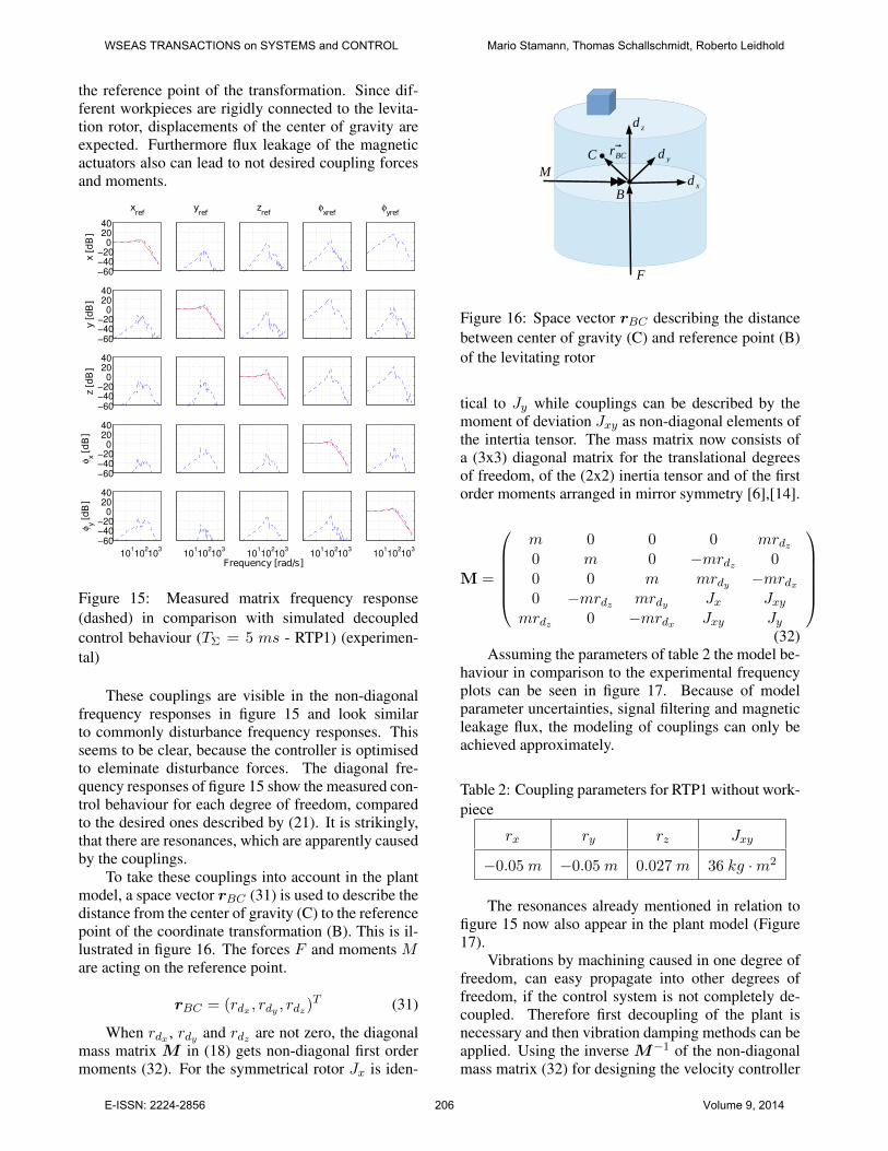
To take these couplings into account in the plantmodel, a space vector rBC (31) is used to describe thedistance from the center of gravity (C) to the referencepoint of the coordinate transformation (B). This is il-lustrated in figure 16. The forces F and moments Mare acting on the reference point.

rBC = (rdx , rdy , rdz)T (31)

When rdx , rdy and rdz are not zero, the diagonalmass matrix M in (18) gets non-diagonal first ordermoments (32). For the symmetrical rotor Jx is iden-

d x

d y

d z

rBCC

B

F

M

Figure 16: Space vector rBC describing the distancebetween center of gravity (C) and reference point (B)of the levitating rotor

tical to Jy while couplings can be described by themoment of deviation Jxy as non-diagonal elements ofthe intertia tensor. The mass matrix now consists ofa (3x3) diagonal matrix for the translational degreesof freedom, of the (2x2) inertia tensor and of the firstorder moments arranged in mirror symmetry [6],[14].

M =

m 0 0 0 mrdz0 m 0 −mrdz 00 0 m mrdy −mrdx0 −mrdz mrdy Jx Jxy

mrdz 0 −mrdx Jxy Jy

(32)

Assuming the parameters of table 2 the model be-haviour in comparison to the experimental frequencyplots can be seen in figure 17. Because of modelparameter uncertainties, signal filtering and magneticleakage flux, the modeling of couplings can only beachieved approximately.

Table 2: Coupling parameters for RTP1 without work-piece

rx ry rz Jxy

−0.05 m −0.05 m 0.027 m 36 kg ·m2

The resonances already mentioned in relation tofigure 15 now also appear in the plant model (Figure17).

Vibrations by machining caused in one degree offreedom, can easy propagate into other degrees offreedom, if the control system is not completely de-coupled. Therefore first decoupling of the plant isnecessary and then vibration damping methods can beapplied. Using the inverse M−1 of the non-diagonalmass matrix (32) for designing the velocity controller


E-ISSN: 2224-2856 206 Volume 9, 2014

−60−40−20

02040

xref

x [d

B]

yref

zref

φxref

φyref

−60−40−20

02040

y [d

B]

−60−40−20

02040

z [d

B]

−60−40−20

02040

φ x[d

B]

10110

210

3−60−40−20

02040

φ y[d

B]

10110

210

310

110

210

3

Frequency [rad/s]10

110

210

310

110

210

3

Figure 17: Simulated coupled control behaviour incomparison to the measured matrix frequency re-sponse (dashed). (TΣ = 5 ms - RTP1) (experimental)

in figure 6, all couplings can be compensated in addi-tion to the mass compensation.

−60−40−20

02040

xref

x [d

B]

yref

zref

φxref

φyref

−60−40−20

02040

y [d

B]

−60−40−20

02040

z [d

B]

−60−40−20

02040

φ x[d

B]

10110

210

3−60−40−20

02040

φ y[d

B]

10110

210

310

110

210

3

Frequency [rad/s]10

110

210

310

110

210

3

Figure 18: Matrix frequency response for the de-coupled feedback control in comparison to figure 15(dashed). (TΣ = 5 ms - RTP1) (experimental)

The measured frequency response plotted in fig-ure 18 shows the control behaviour of the decoupledsystem using the parameters in table 2. Because oftime delay by the current controllers and not exactlyknown parameters, decoupling is only approximatelyreachable. However, in some frequency responses themaximum coupling amplitude could be decreased bymore than 10 dB.

4 Conclusion

This paper has presented the control design for mag-netic bearings as rotary table for mill and drill ma-chining of large and heavy workpieces. Model basedcascade control and sliding mode control concepts foroptimal disturbance rejection in five degrees of free-dom has been shown. The investigation of couplingsin the control structure has figured out, that first de-coupling is necessary to improve the control perfor-mance and establish a basis for vibration damping ofmilling and drilling processes on the table. Furtherresearch needs to be done for online and offline iden-tification of the mass matrix and for decoupling of ex-ternal disturbance forces by drill and mill machining.

Acknowledgements: Investigations of rotary tableprototype 1 was allowed by Experimentelle FabrikMagdeburg, while mill and drill machining on ro-tary table prototype 2 was possible by the support ofthe GMV Genthiner Maschinen- und VorrichtungsbauGmbH company.

References:

[1] C.-R. Sabirin and A. Binder, Rotor levitation byactive magnetic bearing using digital state con-troller, in EPE-PEMC, 2008, pp. 1625-1632.

[2] M. Subkhan and M. Komori, New Concept forFlywheel Energy Storage System Using SMBand PMB, IEEE Transactions on Applied Super-conductivity, vol. 21, 2011, pp. 1485-1488.

[3] S.-O. Siems and W.-R. Canders, Advances inthe design of superconducting magnetic bear-ings for static and dynamic applications, Su-perconductor Science and Technology, 2005, p.S86.

[4] T. Schuhmann, W. Hofmann and R. Werner,Improving Operational Performance of ActiveMagnetic Bearings Using Kalman Filter andState Feedback Control, Industrial Electronics,IEEE Transactions on, vol. 59, 2012, pp. 821-829.

[5] R. Banucu, J. Albert, V. Reinauer, C. Scheiblich,W.-M. Rucker, A. Hafla and A. Huf, Automated


E-ISSN: 2224-2856 207 Volume 9, 2014

Optimization in the Design Process of a Magnet-ically Levitated Table for Machine Tool Applica-tions, IEEE Transactions on Magnetics, vol. 46,2010, pp. 2787-2790.

[6] O. Petzold, Modellbildung und Untersuchungeines magnetisch gelagerten Rundtisches, Dis-sertation Otto von Guericke University Magde-burg, 2006.

[7] D. Schroder, Elektrische Antriebe 2, Regelungvon Antrieben, Springer Verlag Berlin Heidel-berg, 1995

[8] S. Palis, M. Stamann and T. Schallschmidt,Rechnergestutzter Reglerentwurf fur ein Mag-netlager mit Scilab/Scicos-RTAI, EKA Mage-burg, 2008.

[9] M. Stamann, T. Schallschmidt and F. Palis,Aktive Schwingungsdampfung unter Beruck-sichtigung der Nichtlinearitaten am Beispielmagnetisch gelagerter Maschinenrundtische,10. Magdeburger Maschinenbau Fachtagung,2011.

[10] S. Palis, M. Stamann and T. Schallschmidt, Non-linear adaptive control of magnetic bearings,EPE Aalborg, 2007.

[11] T. Schallschmidt, Modellbasierte Regelungmagnetisch gelagerter Rundtische, DissertationOtto von Guericke University Magdeburg, 2012.

[12] V. Utkin, J. Guldner and J. Shi, Sliding ModeControl in Electro-Mechanical Systems, CRCPress by Taylor & Francis Group, 2009.

[13] W. Gao and J.-C. Hung, Variable Structure Con-trol of Nonlinear Systems: A New Approach.,IEEE Transactions on Industrial Electronics,1993.

[14] M. Ruskowski, Aufbau und Regelung aktiverMagnetfuhrungen, Dissertation University Han-nover, 2004.


E-ISSN: 2224-2856 208 Volume 9, 2014

electromagnetic rotary tables for mill and drill · pdf fileelectromagnetic rotary tables for...

Documents