Electromagnetism

Luis Fernando Alday

Chapters

1.- Introduction to Electrostatics

2.- Boundary-value problems in electrostatics

3.- Magnetostatics

4.- Time dependent electromagnetism

5.- Electromagnetic waves

6.- Epilogue: Electromagnetism and special relativity

Reading list

R. Feynman, Lectures in Physics, Vol.2. Electromagnetism, Addison Wesley.

J.D. Jackson, Classical Electrodynamics, John Wiley.

Landau and Lifshitz, The Classical Theory of Fields (to read if you are brave enough!)

1 Introduction to Electrostatics

This is the subject of static electricity, which we’ve all played with: recall rubbing a pen onyour cat and picking up bits of paper. We interpret this as charging up or adding charge tothe pen. As greeks didn’t have pens, they used amber. The greek word for amber is electronand this is where the subject gets its name from.

1.1 Coulomb’s law

We will assume the following facts about charge:

• there exist charges in nature;

• charge can be positive or negative;

• charge cannot be created or destroyed;

For a more sophisticated standpoint, we may know that charge is discrete, and that electronshave charge -1 and protons charge +1 in suitable units, but for our purposes we want tothink of charge as continuous. As a mathematical idealization, we represent charge by areal function, the charge density ρ(x, y, z, t), with the property that the total charge Q in aregion V of space is

Q =

∫V

ρdV =

∫∫∫V

ρ dxdydz. (1)

Other idealizations are possible, and we shall sometimes use them. For example, it may beconvenient to think of charges residing on a surface, something two-dimensional, and thencharge surface density σ(x, y, t) is charge per unit area, so that the total charge on a pieceS of surface is

Q =

∫S

σdS; (2)

similarly, for a one-dimensional distribution of charge, charge line density is charge per unitlength on some curve. Finally, a point charge q corresponds to a finite, nonzero chargelocalized at a point.

After introducing the concept of charge, the natural question is: how do charges interactwith each other? An important experimental fact about point charges is the

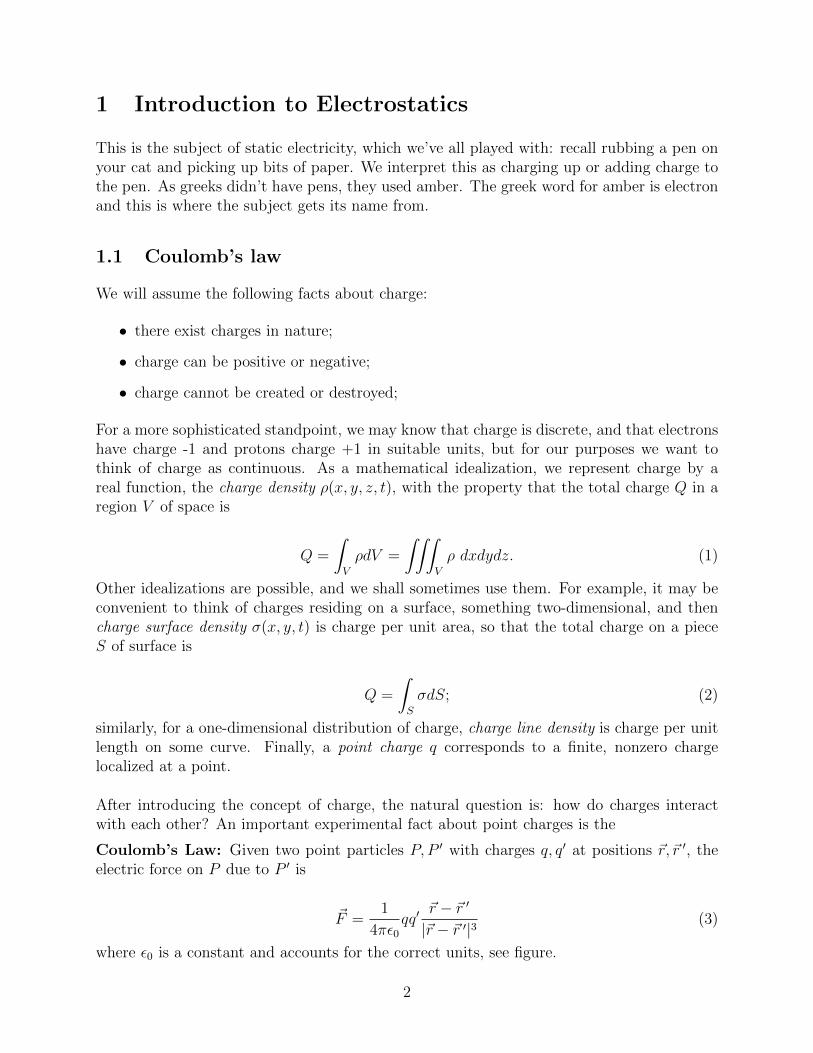
Coulomb’s Law: Given two point particles P, P ′ with charges q, q′ at positions ~r, ~r ′, theelectric force on P due to P ′ is

~F =1

4πε0qq′

~r − ~r ′

|~r − ~r ′|3(3)

where ε0 is a constant and accounts for the correct units, see figure.

2

0

r

r

P

P’

r−r’

We treat this law as an experimental fact. To see how one might have discovered it, notethat:

• it is an inverse-square law, acting along the line joining the particles;

• it is proportional to the product of the charges, so that like charges repel and unlikecharges attract.

1.2 Electric field and scalar potential

It is convenient to think of Coulomb’s law as follows: P ′ generates an electric field to whichP responds. Put P ′ at the origin and define the electric field at ~r to be

~E(~r) =1

4πε0q′~r

r3(4)

Then P , which has charge q, when placed in the field generated by P ′ is subject to (or ”feels”)the force

~F = q ~E (5)

Replace P ′ by various particles P1, P2, ..., Pn, at points ~r1, ~r2, ..., ~rn with charges q1, q2, ..., qn.The forces will add as vectors so if we defined the electric field now as

~E(~r) =1

4πε0

n∑i=1

qi(~r − ~ri)|~r − ~ri|3

, (6)

then, as before, P placed at ~r is subject to the force

~F (~r) = q ~E(~r) (7)

The electric field (6) generalizes easily to the electric field for a volume distribution of chargedensity

~E(~r) =1

4πε0

∫ρ(~r ′)

(~r − ~r ′)|~r − ~r ′|3

dx′dy′dz′, (8)

3

It is instructive to ask how (8) reduces to (6). In order to answer that question we needto understand which charge density ρ(x, y, z) corresponds to a point charge of magnitude qlocated at (x0, y0, z0). This function should be such that it vanishes identically outside thepoint (x0, y0, z0) but at the same time∫

V

ρ(x, y, z)dV = q (9)

for any volume including the point (x0, y0, z0). We introduce the one-dimensional Dirac deltafunction δ(x), defined by the following properties:

1. δ(x) = 0, for x 6= 0

2.∫δ(x)dx = 1, if the region of integration includes x = 0, and is zero otherwise.

Useful properties, which can be derived from the two above are the following:

∫f(x)δ(x− a)dx = f(a), if the region of integration includes x = a, (10)

δ(f(x)) =∑i

1

|f ′(xi)|δ(x− xi), with f(xi) = 0. (11)

In higher dimensions the Dirac delta function is just the product of the cartesian deltafunctions. We see that the volume charge density with the correct properties to correspondto a point charge of magnitude q located at (x0, y0, z0) is given by

ρ(x, y, z) = qδ(~r − ~r0) ≡ qδ(x− x0)δ(y − y0)δ(z − z0) (12)

By using the properties of the delta function you can check that for ρ(~r) =∑qiδ(~r−~ri) (8)

reduces to the potential (6) for a collection of particles.

We want to explore (6). Note first that it is the gradient of another function:

~E = −∇Φ, Φ =1

4πε0

n∑i=1

qi|~r − ~ri|

. (13)

This scalar function Φ is called the electric or scalar potential. The scalar potential has avery nice physical interpretation. Let us think about Newton’s equations of motion for acharged particle of mass m and charge q subject to the force (7)

m~a = ~F = q ~E = −q∇Φ (14)

Then

4

d

dt

(1

2m~v · ~v

)= m~v · ~a = −q~v · ∇Φ = −q

3∑i=1

∂Φ

∂xidxi

dt= −qdΦ

dt(15)

so that

E =1

2m|~v|2 + qΦ = constant (16)

In the motion of the charged particle, the kinetic energy changes with time, but the sumof the kinetic energy and qΦ is constant; thus qΦ is the potential energy of the particle ofcharge q in the electric field with potential Φ. 1

1.3 Gauss law and Poisson equation

In the previous section we have seen that the electric field for a collection of particles is thegradient of a scalar function. In particular, therefore

∇∧ ~E = 0, (17)

From (6) we can also explicitly check

∇ · ~E = ∇2Φ = 0, except at ~r = ~ri (18)

Consider the diagram

P1

P3

P2

S1S3

S2

V

large sphere S

i.e. S is a large sphere containing all Pi, Si is a small sphere containing only Pi and V̂ is theregion in between. Then ∇ · ~E = 0 on V̂ , so

1Note that this is completely analogue to the usual (gravitational) potential energy, the mass m is replacedby the charge q and the potential gh is replaced by the potential Φ.

5

∫S

~E · dS−n∑i=1

∫Si

~E · dS =

∫V̂

∇ · ~EdV = 0 (19)

the first two are surface integrals (with dS pointing away from the center of the correspondingsphere), while the last one is a volume integral. Make sure you understand the signs in thisequation. Let us focus in the integral over S1 and consider only the charge P1. Taking ~r1 = 0for simplicity we obtain:

∫S1

~E · dS =

∫S1

1

4πε0q1~r

r3· ndS

=1

4πε0q1

∫1

r2r2 sin θdθdφ

=1

ε0q1,

in the second step we used n = ~rr. Now, the divergence of the electric field generated by

the other charges vanishes identically inside S1, so we can use the divergence theorem toconclude that they will not contribute to the integral above. Each term in the sum (19) canbe calculated like this, so we obtain:

∫S

~E · dS =n∑i=1

∫Si

~E · dS =1

ε0(q1 + q2 + ...+ qn) =

1

ε0× total charge inside S (20)

This is the Gauss’s Law in its integral form:

Gauss’s Law: The flux of ~E out of V = 1ε0× total charge in V .

If we have a smoothed out charge density instead of point charges, Gauss’s law would read∫S

~E · dS =1

ε0

∫V

ρdV, (21)

where V is the volume inside the closed surface S. We will assume this to be true.

Now, by Divergence theorem we have∫V

(∇ · ~E − 1

ε0ρ

)dV = 0 (22)

but if this is to hold for all possible regions V , then

∇ · ~E =1

ε0ρ, (23)

which is the differential version of Gauss’s Law.

This together with ~E = −∇Φ implies Poisson’s equation

6

∇2Φ = − 1

ε0ρ (24)

What is the solution for this equation? remember that for point particles we had (see (13))

Φ =1

4πε0

n∑i=1

qi|~r − ~ri|

(25)

so we might guess that the solution of (24) is

Φ(~r) =1

4πε0

∫∫∫V

ρ(~r ′)

|~r − ~r ′|dx′dy′dz′ (26)

where V is the region in which ρ 6= 0. In order check that this is the correct guess, we needto apply the Laplacian to both sides. In doing so we are led to consider

∇2

(1

r

)=

1

r

d2

dr2

(r.

1

r

)= 0, for r 6= 0 (27)

At r = 0 we need to be a little bit careful. Indeed, integrating around a little sphere aroundthe origin we find∫

V

∇2

(1

r

)dV =

∫V

∇ · ∇(

1

r

)dV =

∫S

n · ∇(

1

r

)ds = −4π (28)

hence we arrive to the following beautiful equation

∇2

(1

|~r − ~r ′|

)= −4πδ(~r − ~r ′) (29)

using this it is immediate to check that (26) is a solution to the Poisson equation. Incidentally,also note that (29) implies the Poisson equation also works for point charges, where the chargedensity has the form (12).

An example

The main problem of Electrostatics is to obtain ~E given the charge distribution. We havesolved that problem with (26): Given the density ρ, integrate this to find Φ and then~E = −∇Φ. However, in simple cases we can go straight to ~E by using (4). Here is anexample:

Total charge Q is spread out uniformly round a plane circular wire of radius a. Find theelectric field at a point P on the axis of the circle, at a distance b from the centre.

7

L

P

b

a

α

k

e

unit vectors

We can do this one directly from the inverse square law: ~E = q4πε0

~rr3

.

Cut the circular wire into elements, each of length adθ; then each contains charge equal toQ2πdθ and so contributes Q

2πdθ 1

4πε0~eL2 , (with ~e as in the figure) to ~E at P . Adding these up

around the circle leads, by symmetry, to a vector along ~k. Note, from the diagram, that~e · ~k = cosα, so that ~E(p) = E~k, with E a scalar and given by

E =

∫Q

2π· dθ · 1

4πε0· cosα

L2

=Q

4πε0

cosα

L2

=Q

4πε0

b

(a2 + b2)3/2

which is the answer.

It is trickier to find ~E for a point P ′ not on the axis.

Another example: Discontinuity as you cross a surface density

Suppose we want to compute the discontinuity in the electric field as we cross a surface layerof charge, with surface density σ(x, y), see figure.

8

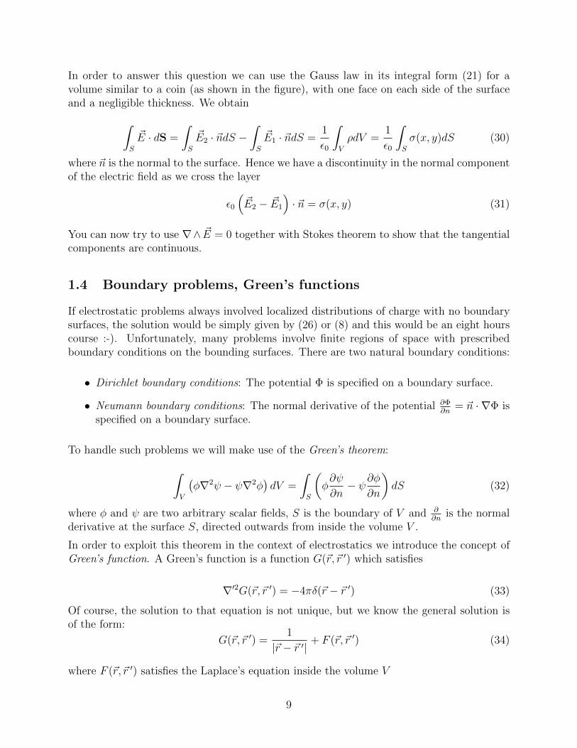
In order to answer this question we can use the Gauss law in its integral form (21) for avolume similar to a coin (as shown in the figure), with one face on each side of the surfaceand a negligible thickness. We obtain∫

S

~E · dS =

∫S

~E2 · ~ndS −∫S

~E1 · ~ndS =1

ε0

∫V

ρdV =1

ε0

∫S

σ(x, y)dS (30)

where ~n is the normal to the surface. Hence we have a discontinuity in the normal componentof the electric field as we cross the layer

ε0

(~E2 − ~E1

)· ~n = σ(x, y) (31)

You can now try to use ∇∧ ~E = 0 together with Stokes theorem to show that the tangentialcomponents are continuous.

1.4 Boundary problems, Green’s functions

If electrostatic problems always involved localized distributions of charge with no boundarysurfaces, the solution would be simply given by (26) or (8) and this would be an eight hourscourse :-). Unfortunately, many problems involve finite regions of space with prescribedboundary conditions on the bounding surfaces. There are two natural boundary conditions:

• Dirichlet boundary conditions: The potential Φ is specified on a boundary surface.

• Neumann boundary conditions: The normal derivative of the potential ∂Φ∂n

= ~n · ∇Φ isspecified on a boundary surface.

To handle such problems we will make use of the Green’s theorem:∫V

(φ∇2ψ − ψ∇2φ

)dV =

∫S

(φ∂ψ

∂n− ψ∂φ

∂n

)dS (32)

where φ and ψ are two arbitrary scalar fields, S is the boundary of V and ∂∂n

is the normalderivative at the surface S, directed outwards from inside the volume V .

In order to exploit this theorem in the context of electrostatics we introduce the concept ofGreen’s function. A Green’s function is a function G(~r, ~r ′) which satisfies

∇′2G(~r, ~r ′) = −4πδ(~r − ~r ′) (33)

Of course, the solution to that equation is not unique, but we know the general solution isof the form:

G(~r, ~r ′) =1

|~r − ~r ′|+ F (~r, ~r ′) (34)

where F (~r, ~r ′) satisfies the Laplace’s equation inside the volume V

9

∇′2F (~r, ~r ′) = 0 (35)

we will use the freedom to choose F (~r, ~r ′) momentarily. Next, let us consider Green’s theoremwith φ = Φ(~r ′) the scalar potential and ψ = G(~r, ~r ′) the Green’s function. We obtain

∫V

(Φ(~r ′)∇′2G(~r, ~r ′)−G(~r, ~r ′)∇′2Φ(~r ′)

)dV ′ =

∫S

(Φ(~r ′)

∂G(~r, ~r ′)

∂n′−G(~r, ~r ′)

∂Φ(~r ′)

∂n′

)dS ′(36)

Using (33) and the properties of the delta function we obtain∫V

Φ(~r ′)∇′2G(~r, ~r ′)dV ′ = −4πΦ(~r) (37)

where we have assumed that the observation point ~r is inside the volume V . In this case weobtain

Φ(~r) =1

4πε0

∫V

ρ(~r ′)G(~r, ~r ′)dV ′ +1

4π

∫S

(G(~r, ~r ′)

∂Φ(~r ′)

∂n′− Φ(~r ′)

∂G(~r, ~r ′)

∂n′

)dS ′ (38)

Now we can use the freedom in the definition of the Green’s function. If we are solving aproblem with Dirichlet boundary conditions we demand

GD(~r, ~r ′) = 0, for ~r ′ in S. (39)

Once we have found a Green’s function with these boundary conditions, the solution for thepotential is simply given by

Φ(~r) =1

4πε0

∫V

ρ(~r ′)GD(~r, ~r ′)dV ′ − 1

4π

∫S

(Φ(~r ′)

∂GD(~r, ~r ′)

∂n′

)dS ′ (40)

For Neumann boundary conditions we must be more careful. We cannot require the normalderivative of G to vanish: application of the Gauss theorem to the definition of Green’sfunction gives ∫

S

∂G(~r, ~r ′)

∂nds′ = −4π (41)

The easiest condition we can require is

∂GN(~r, ~r ′)

∂n= −4π

A(42)

where A is the total surface area of S. Then the solution is

Φ(~r) = 〈Φ〉S +1

4πε0

∫V

ρ(~r ′)GN(~r, ~r ′)dV ′ +1

4π

∫S

GN(~r, ~r ′)∂Φ(~r ′)

∂n′dS ′ (43)

10

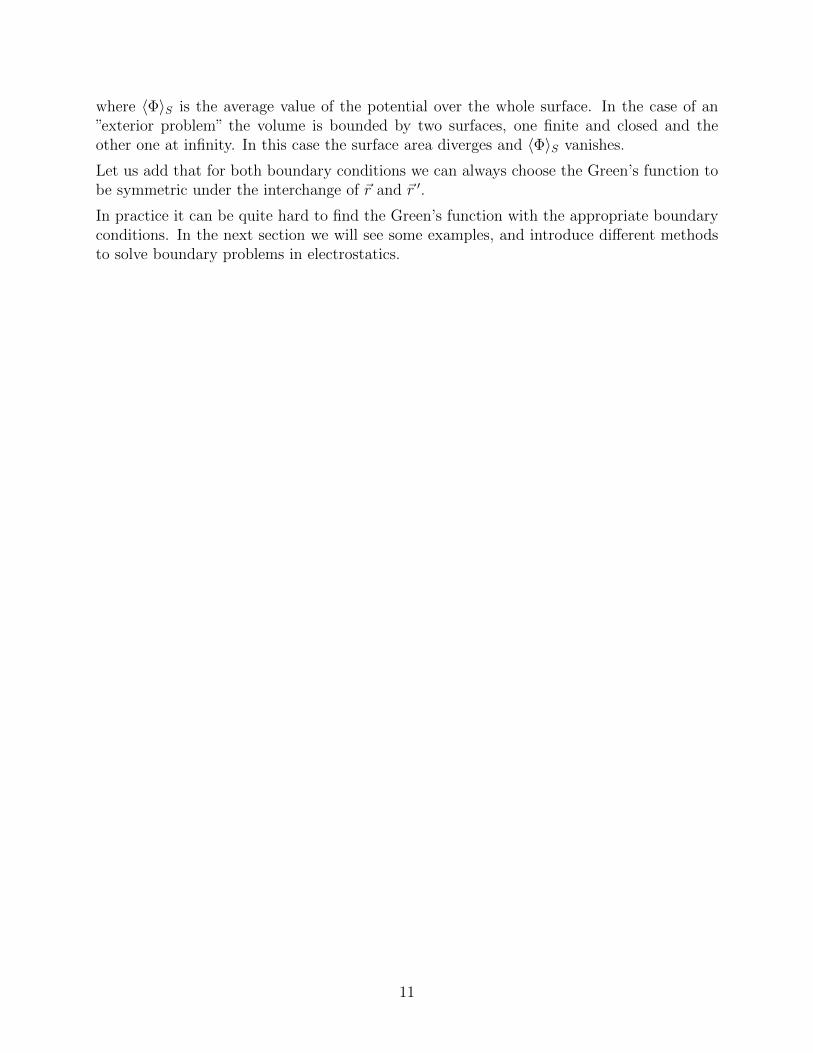
where 〈Φ〉S is the average value of the potential over the whole surface. In the case of an”exterior problem” the volume is bounded by two surfaces, one finite and closed and theother one at infinity. In this case the surface area diverges and 〈Φ〉S vanishes.

Let us add that for both boundary conditions we can always choose the Green’s function tobe symmetric under the interchange of ~r and ~r ′.

In practice it can be quite hard to find the Green’s function with the appropriate boundaryconditions. In the next section we will see some examples, and introduce different methodsto solve boundary problems in electrostatics.

11

2 Boundary-value problems in electrostatics

Many problems in electrostatics involve boundary surfaces on which either the potential orthe normal derivative of the potential is specified. We have already obtained the formal solu-tion to such problems by the method of Green’s functions. To find such functions, however,can be quite complicated, and several methods have been developed to solve boundary-valueproblems in electrostatics. In this chapter we will see some of them.

2.1 Method of images

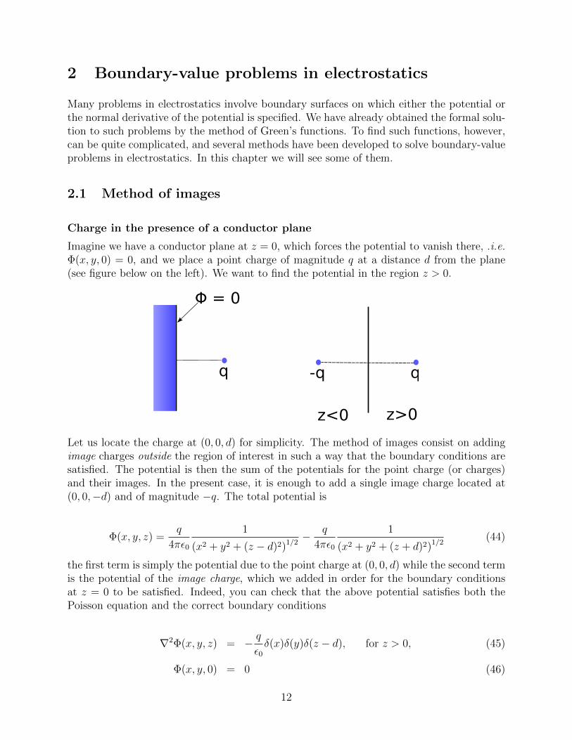
Charge in the presence of a conductor plane

Imagine we have a conductor plane at z = 0, which forces the potential to vanish there, .i.e.Φ(x, y, 0) = 0, and we place a point charge of magnitude q at a distance d from the plane(see figure below on the left). We want to find the potential in the region z > 0.

q q-q

Φ = 0

z>0z<0

Let us locate the charge at (0, 0, d) for simplicity. The method of images consist on addingimage charges outside the region of interest in such a way that the boundary conditions aresatisfied. The potential is then the sum of the potentials for the point charge (or charges)and their images. In the present case, it is enough to add a single image charge located at(0, 0,−d) and of magnitude −q. The total potential is

Φ(x, y, z) =q

4πε0

1

(x2 + y2 + (z − d)2)1/2− q

4πε0

1

(x2 + y2 + (z + d)2)1/2(44)

the first term is simply the potential due to the point charge at (0, 0, d) while the second termis the potential of the image charge, which we added in order for the boundary conditionsat z = 0 to be satisfied. Indeed, you can check that the above potential satisfies both thePoisson equation and the correct boundary conditions

∇2Φ(x, y, z) = − qε0δ(x)δ(y)δ(z − d), for z > 0, (45)

Φ(x, y, 0) = 0 (46)

12

Note that it is important that the image charge is located outside the region of interest (seefigure above on the right), hence the total potential will still satisfy the Poisson equation inthe region of interest. More precisely, we could have added the delta function correspondingto the image charge, but this vanishes identically for z > 0.

The method of images is intimately connected to the method of Green’s functions. In order tomake this relation clear, let us solve this problem by using the method of Green’s functions.The Green’s functions for Dirichlet boundary conditions on the plane z = 0 take the form

G(~r, ~r ′) =1

|~r − ~r ′|+ F (~r, ~r ′), ∇′2F (~r, ~r ′) = 0, z, z′ > 0 (47)

where F (~r, ~r ′) has to be chosen such as to satisfy

G(~r, ~r ′) = 0, for z′ = 0. (48)

we can choose

F (~r, ~r ′) = − 1

|~r − ~r ′R|(49)

where ~r ′R is the reflection of ~r ′ on the plane, namely ~r ′R = (x′, y′,−z′). Note that in theregion of interest the Laplacian of F (~r, ~r ′) vanishes. The relation with the method of imagesis now clear, the Green’s function for Dirichlet boundary conditions on z = 0

GD(~r, ~r ′) =1

|~r − ~r ′|− 1

|~r − ~r ′R|(50)

is simply the potential for a point charge of unit magnitude (in units of 4πε0) in the presenceof a conductor plane at z = 0, where ~r ′ is the location of the point charge. This has to bethe case, indeed, by definition the Green’s function satisfies the Poisson equation with a unitcharge as a source and vanishes at z = 0. 2

Having constructed the appropriate Green’s function we can now plug the desired chargedistribution in (40). For example, for a point charge at ~d we obtain

Φ(~r) = q

∫V

δ(~r ′ − ~d )

(1

|~r − ~r ′|− 1

|~r − ~r ′R|

)dV ′ =

q

|~r − ~d|− q

|~r − ~dR|(51)

exactly as expected from the method of images.

Returning to the potential (44) there are many questions we can ask. For instance, what isthe force acting on the charge q? the simplest way to calculate this is by computing the forcedone on the charge q by its image, an attractive force along the z direction with magnitude

|Fz| =1

4πε0

q2

4d2(52)

2Note that the Green’s function is symmetric under interchange of ~r and ~r ′, so it also vanishes for z′ = 0,which was the original requirement for Green’s functions in section one.

13

There is another, more instructive, way to compute the force. Though the potential vanishesat z = 0 its normal derivative does not:

∂

∂zΦ|z=0 =

1

2πε0

q d

(x2 + y2 + d2)3/2(53)

Through (31) we can interpret this result as saying that the charge is inducing a surfacedensity:

σ(x, y) = − 1

2π

q d

(x2 + y2 + d2)3/2(54)

An infinitesimal piece of surface dxdy possesses total charge σ(x, y)dxdy, hence the totalforce over the charge is

Fz =q

4πε0

∫σ(x, y)

d

(x2 + y2 + d2)3/2dxdy = − 1

4πε0

q2

4d2(55)

In perfect agreement with our previous result.

In the following we will discuss another geometry where it is possible to guess the locationof the image charges.

Charge in the presence of a conductor sphere

Imagine we place a point charge of magnitude q at a distance b from the center of a sphere ofradius a < b. The sphere is a grounded conductor, so we require the potential to vanish onits surface, namely Φ(~r) = 0 for |~r| = a. We want to find the potential for this configurationin the region |~r| > a (see figure).

q

Φ = 0

q'

14

Let us denote the vector position of the point charge as ~rq = nqb and let us assume that onlyone image charge of magnitude q′ is enough. By symmetry, the image charge should lie onthe ray from the origin to the original point charge. The scalar potential would then be

Φ(~r) =1

4πε0

(q

|~r − nqb|+

q′

|~r − nqb′|

)(56)

Now we need to adjust q′ and b′ such that

Φ(na) =1

4πε0

(q

|na− nqb|+

q′

|na− nqb′|

)= 0 (57)

for any unit vector n. You can explicitly check that this can be achieved by choosing

q′ = −abq, b′ =

a2

b(58)

Which gives the full potential for the problem at hand

Φ(~r) =1

4πε0

(q

|~r − nqb|− a

b

q

|~r − nqa2/b|

)(59)

Green’s function for the sphere

As for the case of the conductor plane, the Dirichlet Green’s function for the sphere is simplythe potential for a unit charge (including its image) in units of 4πε0, where ~r ′ refers to thelocation of the unit charge. We obtain

G(~r, ~r ′) =1

|~r − ~r ′|− a

r ′1

|~r − a2

r′2~r ′|

=1

(r2 + r′2 − 2rr′ cos γ)1/2− 1(

r2r′2

a2+ a2 − 2rr′ cos γ

)1/2

(60)where γ is the angle between ~r and ~r ′. With the Green’s function at our disposal, we canwrite down the general solution to the Dirichlet problem on the sphere. For instance, supposefor simplicity that there is no charge distribution and the prescribed boundary conditionsat the sphere fix Φ(a, θ, φ) = V (θ, φ), where we are using spherical coordinates. Then, from(40), the solution to the potential takes the form

Φ(~r) =1

4π

∫V (θ′, φ′)

a(r2 − a2)

(r2 + a2 − 2ar cos γ)3/2sin θ′dθ′dφ′ (61)

2.2 Method of orthonormal functions

A very important feature of the equations of electrostatics, (17) and (23) or equivalently (24),is that they are linear equations (in the fields or the potential). This leads to the principleof superposition: the sum of solutions is also a solution. Conversely any solution can also be

15

expressed in a convenient basis of solutions (you have already met this phenomenon, whensolving the equations of motion for a vibrating string).

The representation of solutions of potential problems by expansions in orthonormal functionsis a powerful technique that can be used in a large class of problems. The particular setchosen depends on the symmetries of the problem.

Generalities

We start by recalling some general properties of orthonormal functions. Consider an inter-val (a, b) and a set of real or complex functions in one variable Un(x), n = 1, 2, .... Theorthonormality condition takes the form

∫ b

a

U∗m(x)Un(x)dx = δmn (62)

If the above set is complete then an arbitrary function f(x) (square integrable in the interval(a, b)) can be written as a linear combination of the orthonormal functions

f(x) =∞∑n=1

anUn(x) (63)

where the coefficients are given by

an =

∫ b

a

U∗n(x)f(x)dx (64)

Plugging this expression into (63) we obtain

f(x) =

∫ b

a

(∞∑n=1

U∗n(x′)Un(x)

)f(x′)dx′ (65)

recalling the properties of the Dirac delta function, it should be the case that

∞∑n=1

U∗n(x′)Un(x) = δ(x′ − x) (66)

This is called completeness or closure relation. The most famous example of orthogonalfunctions are the sines and cosines that enter in the Fourier expansion. For the interval(−a/2, a/2) they are √

2

asin

(2πnx

a

),

√2

acos

(2πnx

a

)(67)

The extension to higher dimensions is obvious. For instance, a function of two variablesadmits an expansion in terms of the sets Un(x) and Vn(y).

16

f(x, y) =∑

amnUm(x)Vn(y), where amn =

∫dx

∫dy U∗m(x)V ∗n (y)f(x, y) (68)

If the interval becomes infinite the set of orthogonal functions Un(x) may become an uncount-able set, namely Un(x) → Uk(x) with k a real number. In this case sums are replaced byintegrals and the Kronecker delta is replaced by the Dirac delta. The most famous exampleis the exponential Fourier series expansion in terms of the set

Uk(x) =1√2πeikx (69)

An arbitrary function can be expanded in terms of those

f(x) =1√2π

∫ ∞−∞

A(k)eikxdk (70)

This expansion is usually called exponential Fourier expansion. The ”coefficients” A(k)(which now depend on a continuous function) are given by

A(k) =1√2π

∫ ∞−∞

e−ikxf(x)dx (71)

The orthonormality condition is

1

2π

∫ ∞−∞

ei(k−k′)xdx = δ(k − k′) (72)

while the completeness relation takes the form

1

2π

∫ ∞−∞

eik(x−x′)dk = δ(x− x′) (73)

These last two integrals give useful representations of the delta function, and will be usedbelow.

Cartesian coordinates

For electrostatic problems with rectangular symmetries it is convenient to use cartesiancoordinates. The Laplace equation in cartesian coordinates is

∂2Φ

∂x2+∂2Φ

∂y2+∂2Φ

∂z2= 0 (74)

Looking for separable solutions of the form Φ(x, y, z) = X(x)Y (y)Z(z) we find

1

X(x)

d2X

dx2+

1

Y (y)

d2Y

dy2+

1

Z(x)

d2Z

dz2= 0 (75)

17

which implies

1

X(x)

d2X

dx2= −α2,

1

Y (y)

d2Y

dy2= −β2,

1

Z(x)

d2Z

dz2= α2 + β2 (76)

Hence we find the following basis of solutions

Φ = e±iαxe±iβye±√α2+β2z (77)

where at this point α and β are arbitrary, but we have chosen them to be real. Any linearcombination of the above solutions is a solution. When specific boundary conditions areimposed on the potential, we will have a restriction on the values that α and β can take.

For example, let us consider the problem of finding the potential inside a rectangular boxwith dimensions (a, b, c) in the (x, y, z) directions, such that the potential vanishes at allfaces except at z = c, where it takes some prescribed value Φ(x, y, c) = V (x, y), see figure.

Φ = V(x,y)

a b

c

Requiring the potential to vanish at x = 0, y = 0 and z = 0 we see the potential should bethe sum of terms of the form

Φ = sinαx sin βy sinh√α2 + β2z (78)

Requiring the potential to vanish at x = a and y = b further fixes the form of α and β

α =mπ

a, β =

nπ

b(79)

for m,n integer numbers. Hence, requiring the boundary conditions on five of the six facesfixes the form of the solution to be

18

Φ(x, y, z) =∞∑

m,n=1

Am,n sin(mπax)

sin(nπby)

sinh

√(mπa

)2

+(nπb

)2

z (80)

The remaining boundary condition requires

∞∑m,n=1

Am,n sin(mπax)

sinnπ

by sinh

√(mπa

)2

+(nπb

)2

c = V (x, y) (81)

Which is basically the sine Fourier expansion of V (x, y). Hence the coefficients Am,n aregiven by

Am,n =4

ab sinh√(

mπa

)2+(nπb

)2c

∫ a

0

dx

∫ b

0

dy sinmπ

ax sin

nπ

byV (x, y) (82)

where we have considered an odd extension of V 3 and used the orthonormality of the func-tions entering the solution:∫ a

−adx sin

(mπax)

sin

(m′π

ax

)= aδmm′ (83)

for m 6= 0.

Another problem which can be easily solved by the method of rectangular orthogonal func-tions is that of a point charge q inside a grounded box. Imagine the potential is requiredto vanish at the six faces x, y, z = 0 and x = a, y = b, z = c, and we locate a charge q at(x0, y0, z0). The potential should satisfy the corresponding Poisson equation

∇2Φ(x, y, z) = − qε0δ(x− x0)δ(y − y0)δ(z − z0) (84)

The boundary conditions suggest we expand the solution in terms of the set of orthogonalfunctions

Φ(x, y, z) =∞∑

m,n,`=1

Am,n,`

√8

abcsin(mπx

a

)sin(nπy

b

)sin

(`πz

c

)(85)

Note that the boundary conditions are automatically satisfied. Plugging this expression intothe right hand side of the Poisson equation (84) we find

−∞∑

m,n,`=1

Am,n,`

√8

abc

((mπa

)2

+(nπb

)2

+

(`π

c

)2)

sin(mπx

a

)sin(nπy

b

)sin

(`πz

c

)(86)

3Remember from Fourier series, in order to do a sine expansion often you have to extend your functionsto the region (−a, 0) in a fashion consistent with the odd symmetry of sinx.

19

On the other hand, using the completeness relation (66) for the orthonormal functions athand gives the following representation of the delta function

δ(x− x0) =∞∑m=1

2

asin(mπx

a

)sin(mπx0

a

)(87)

and similar for δ(y − y0) and δ(z − z0). We see the Poisson equation is satisfied if

Am,n,` =q

ε0

√8

abc

((mπa

)2

+(nπb

)2

+

(`π

c

)2)−1

sin(mπx0

a

)sin(nπy0

b

)sin

(`πz0

c

)which gives the final solution

Φ(x, y, z) =q

ε0

∞∑m,n,`=1

8

abc

sin(mπx0a

)sin(nπy0b

)sin(`πz0c

)(mπa

)2+(nπb

)2+(`πc

)2 sin(mπx

a

)sin(nπy

b

)sin

(`πz

c

)It would have been extremely hard to solve this problem by other methods!

Finally, in order to solve problems with boundary surfaces it is sometimes convenient toexpand the corresponding Green’s function in the particular set of orthonormal functionsunder consideration. For instance, lets consider Dirichlet boundary conditions at the planez = 0. We have already found the Green’s function for this problem and have obtained

G(~r, ~r ′) =1

|~r − ~r ′|− 1

|~r − ~r ′R|(88)

In order to expand this in rectangular orthonormal functions, recall the integral representa-tion (73) for the Dirac delta function

1

(2π)3

∫ ∞−∞

dα

∫ ∞−∞

dβ

∫ ∞−∞

dγeiαxeiβyeiγz = δ(x)δ(y)δ(z) (89)

This suggests

−4π

(2π)3

∫ ∞−∞

dα

∫ ∞−∞

dβ

∫ ∞−∞

dγeiαxeiβyeiγz

α2 + β2 + γ2=

1

(x2 + y2 + z2)1/2(90)

Since acting with the Laplacian would produce −4πδ(~r) on both sides. Integrating over γwe obtain

1

(x2 + y2 + z2)1/2= − 1

2π

∫ ∞−∞

dα

∫ ∞−∞

dβeiαxeiβye−|z|√α2+β2√

α2 + β2(91)

Hence we obtain for the Green’s function

1

|~r − ~r ′|− 1

|~r − ~r ′R|= − 1

2π

∫ ∞−∞

dα

∫ ∞−∞

dβeiα(x−x′)eiβ(y−y′)√

α2 + β2

(e−|z−z

′|√α2+β2 − e−|z+z′|

√α2+β2

)(92)

20

As expected, note that the r.h.s. vanishes if either z = 0 or z′ = 0.

Spherical coordinates

The Laplace equation in spherical coordinates (r, θ, φ) takes the form

1

r

∂2

∂r2(rΦ) +

1

r2 sin θ

∂

∂θ

(sin θ

∂Φ

∂θ

)+

1

r2 sin2 θ

∂2Φ

∂φ2= 0 (93)

Note that the Laplacian splits into a ”radial” part and an ”angular” part

∇2Φ =1

r

∂2

∂r2(rΦ) +

1

r2∇2θ,φΦ (94)

∇2θ,φ =

1

sin θ

∂

∂θ

(sin θ

∂Φ

∂θ

)+

1

sin2 θ

∂2Φ

∂φ2(95)

It is convenient to look for separable solutions of the form

Φ(r, θ, φ) = R(r)Y (θ, φ) (96)

Proceeding as before, we find the expansion in terms of orthonormal functions takes the form

Φ =∞∑`=0

∑̀m=−`

(A`,mr

` +B`,mr−(`+1)

)Y`m(θ, φ) (97)

The orthonormal functions Y`m(θ, φ) depend only on the angular variables and are calledspherical harmonics. Here ` = 0, 1, 2, ... and for a fixed ` , m takes the integer values from−m to m. They satisfy

∇2θ,φY`m(θ, φ) = −`(`+ 1)Y`m(θ, φ) (98)

This is a complete set of functions, in the sense that any (single valued!) function of theangular variables g(θ, φ) can be written in terms of those. They satisfy

Y`,−m(θ, φ) = (−1)mY ∗`,m(θ, φ) (99)

The orthonormality condition takes the form∫ 2π

0

dφ

∫ π

0

sin θdθY ∗`′,m′(θ, φ)Y`,m(θ, φ) = δ`,`′δm,m′ (100)

while the completeness relation takes the form

∞∑`=0

∑̀m=−`

Y ∗`,m(θ′, φ′)Y`,m(θ, φ) = δ(φ− φ′)δ(cos θ − cos θ′) (101)

21

The first few spherical harmonics are

Y00 =1√4π

(102)

Y11 = −√

3

8πsin θeiφ (103)

Y10 =

√3

4πcos θ (104)

Y22 =1

4

√15

2πsin2 θe2iφ (105)

Y21 = = −√

15

8πsin θ cos θeiφ (106)

Y20 =

√5

4π

(3

2cos2 θ − 1

2

)(107)

The prototypical problem with spherical symmetry is that of finding the potential inside asphere of radius a with prescribed potential at the sphere. Namely the potential satisfies theLaplace equation and the boundary conditions

Φ(a, θ, φ) = V (θ, φ) (108)

Φ(r, θ, φ) is bounded as r → 0 (109)

Where V (θ, φ) is some prescribed function. The general solution to this problem takes theform

Φ(r, θ, φ) =∞∑`=0

∑̀m=−`

A`,mr`Y`m(θ, φ) (110)

where we have used the fact that the solution is bounded as r → 0, so as to keep onlynon-negative powers or r. Note that if we were interested in solving the problem outside thesphere, we would require that the potential is bounded at infinity, and we would keep onlythe negative powers. The coefficients A`,m can be fixed by requiring the correct boundaryconditions at r = a:

Φ(a, θ, φ) =∞∑`=0

∑̀m=−`

A`,ma`Y`m(θ, φ) = V (θ, φ) (111)

Using the orthonormality condition (100) we obtain

A`,m =

∫ 2π

0

dφ

∫ π

0

sin θdθY ∗`,m(θ, φ)V (θ, φ) (112)

22

As in the case of rectangular coordinates, for problems including boundaries, it will beuseful to expand the Dirichlet Green’s function for a sphere of radius a in terms of sphericalorthonormal functions

G(~r, ~r ′) =∑`,m

A`,mY`,m(θ, φ) (113)

where (θ, φ) are the angular coordinates of the point r and the ”coefficients”A`,m depend on(r, r′, θ′, φ′). Since the l.h.s is symmetric under interchange of ~r and ~r ′ we can furthermorewrite

G(~r, ~r ′) =∑`,m

Y ∗`,m(θ′, φ′)A`,m(r, r′)Y`,m(θ, φ) (114)

In order to compute the coefficients A`,m(r, r′) we can proceed as follows. The Dirac deltafunction in spherical coordinates takes the form 4

δ(~r − ~r ′) =1

r2δ(r − r′)δ(φ− φ′)δ(cos θ − cos θ′) (115)

Using the completeness relation (101) we can write

δ(~r − ~r ′) =∞∑`=0

∑̀m=−`

1

r2δ(r − r′)Y ∗`,m(θ′, φ′)Y`,m(θ, φ) (116)

hence

∇2∑`,m

Y ∗`,m(θ′, φ′)A`,m(r, r′)Y`,m(θ, φ) = −4π∞∑`,m

1

r2δ(r − r′)Y ∗`,m(θ′, φ′)Y`,m(θ, φ) (117)

which implies1

r

d2

dr2(rA`,m)− `(`+ 1)

r2A`,m = −4π

r2δ(r − r′) (118)

For the regions r > r′ and r < r′ the delta function vanishes and we obtain

A`,m(r, r′) =

Ar` +Br−(`+1), r < r′

A′r` +B′r−(`+1), r > r′(119)

Now we need to fix the constants of integration A,B,A′, B′ (careful: since the equation ison r, these constants could actually depend on r′). Remember that we interpret ~r as theobservation point and ~r ′ as the location of the unit point charge. Since the Green’s function

4To express δ(x−x′) = δ(x1−x′1)δ(x2−x′2)δ(x3−x′3) in terms of coordinates another set of coordinates(y1, y2, y3) we need to divide by the Jacobian, so that δ(x− x′)d3x is invariant.

23

is bounded as we take the observation point to infinity, we need A′ = 0. Furthermore, theGreen’s function vanishes as r = a, which gives a relation between A and B and continuityat r = r′ leave us only with an overall constant

A`,m(r, r′) =

A(r` − a2`+1

r(`+1)

), r < r′

A(r′2`+1 − a2`+1

)r−(`+1), r > r′

(120)

The overall constant can be fixed as follows. Multiplying (118) by r and integrating bothsides over the interval r = r′ − ε to r = r′ + ε we obtain[

d

dr(rA`,m(r, r′))

]r′+ε

−[d

dr(rA`,m(r, r′))

]r′−ε

= −4π

r′(121)

from where it follows

A = 4πr′−(`+1)

2`+ 1(122)

Putting all together we can write the Green’s function as

G(~r, ~r ′) = 4π∑`,m

1

2`+ 1

(r`< −

a2`+1

r`+1<

)r−(`+1)> Y ∗`,m(θ′, φ′)Y`,m(θ, φ) (123)

where r> and r< denote the bigger and smaller between r and r′. Note that the Green’sfunction vanishes for both r = a and r′ = a (when one of the the two conditions is satisfied,the other radius is bigger, since we are looking at the sphere from outside). In very muchthe same way one can work out The Green’s function for the interior of the sphere. In thiscase we obtain

G(~r, ~r ′) = 4π∑`,m

1

2`+ 1r`<

(r−(`+1)> − r`>

a2`+1

)Y ∗`,m(θ′, φ′)Y`,m(θ, φ) (124)

24

3 Magnetostatics

Frequently, people find magnetism a little more mysterious than electricity. Rather thanthinking of fridge magnets, you should think of electromagnets: charges in motion give riseto electric currents and these produce magnetic fields; many of you will have visualizedthese fields in experiments by sprinkling iron filings on sheets of cardboard transverse to acurrent-carrying wire. (The fridge magnet, or any permanent magnet, derives its magnetismfrom microscopic currents.) The subject corresponding to electrostatics, which is producedby time-independent charges, is magnetostatics, which is produced by time-independent, or”steady”, currents.

+ v

+ v

+ v

+ v

+ v

Given a collection of point chargesQi in motion with velocities ~vi, we define the correspondingelectric currents as:

~j =∑

qi~vi

This is a vector field made by adding up elementary contributions. By analogy with chargedensity ρ as a smoothed-out distribution of point charges, we introduce a vector field, thecurrent density ~J(x, y, z, t), so that the total electric current in a region V is the integral∫V~JdV .

In this section we shall usually be thinking of steady currents, but there is one thing to dealwith first, namely the mathematical expression for the physical observation than charge isconserved.

3.1 Conservation of charge

Consider a region V with surface S with charges moving through.

V

S

25

The total charge inside V is Q =∫VρdV , so that

dQ

dt=

∫V

∂ρ

∂tdV allowing ∂ρ

∂t6= 0 for the moment

= rate of increase of Q

= rate charge goes in− rate charge goes out

= −∫S

~J · dS

= −∫V

∇ · ~JdV by divergence theorem

an so ∫V

(∂ρ

∂t+∇ · ~J

)dV = 0 (125)

this is to be true for all regions V , then

∂ρ

∂t+∇ · ~J = 0 (126)

which is the charge conservation equation.

For the rest of this section, we suppose none of the quantities of interest depends on time.For this time independent situation (126) reduces to ∇ · ~J = 0.

3.2 Magnetic Field Strength

Like the electric field ~E, the magnetic field strength ~B can be defined from an experimentallystablished force law. Analogously to (7), a charged particle with charge q, moving with

velocity ~v in a magnetic field ~B is subject to a force

~F = q~v ∧ ~B (127)

F

B

v

26

This serves to define ~B, but note a peculiar feature of this force law, that the force isorthogonal to the velocity. In particular, therefore ~v · ~F = 0 and the force does no work.

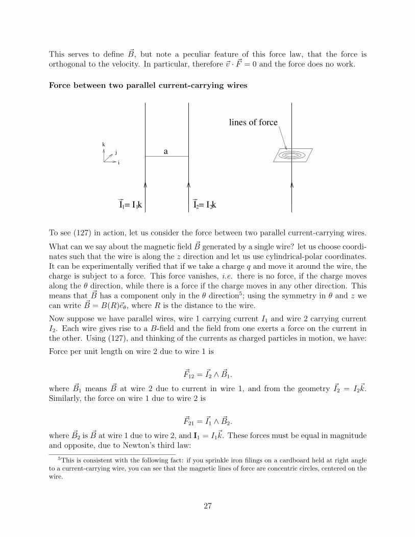
Force between two parallel current-carrying wires

1I = I k1 2I = I k2

k

i

j a

lines of force

To see (127) in action, let us consider the force between two parallel current-carrying wires.

What can we say about the magnetic field ~B generated by a single wire? let us choose coordi-nates such that the wire is along the z direction and let us use cylindrical-polar coordinates.It can be experimentally verified that if we take a charge q and move it around the wire, thecharge is subject to a force. This force vanishes, i.e. there is no force, if the charge movesalong the θ direction, while there is a force if the charge moves in any other direction. Thismeans that ~B has a component only in the θ direction5; using the symmetry in θ and z wecan write ~B = B(R)~eθ, where R is the distance to the wire.

Now suppose we have parallel wires, wire 1 carrying current I1 and wire 2 carrying currentI2. Each wire gives rise to a B-field and the field from one exerts a force on the current inthe other. Using (127), and thinking of the currents as charged particles in motion, we have:

Force per unit length on wire 2 due to wire 1 is

~F12 = ~I2 ∧ ~B1.

where ~B1 means ~B at wire 2 due to current in wire 1, and from the geometry ~I2 = I2~k.

Similarly, the force on wire 1 due to wire 2 is

~F21 = ~I1 ∧ ~B2.

where ~B2 is ~B at wire 1 due to wire 2, and I1 = I1~k. These forces must be equal in magnitude

and opposite, due to Newton’s third law:

5This is consistent with the following fact: if you sprinkle iron filings on a cardboard held at right angleto a current-carrying wire, you can see that the magnetic lines of force are concentric circles, centered on thewire.

27

~I2 ∧ ~B1 = −~I1 ∧ ~B2.

From what was said about the direction of ~B, we have that at wire 2, ~B1 = ~jB1 in terms ofsome magnitude B1, and in wire 1, ~B2 = −~jB2 in terms of some magnitude B2. Therefore

|~F12| = I2B1 = |F21| = I1B2.

It is an experimental fact that this magnitude is

|~F | = µ0

2πaI1I2

in terms of a constant µ0 (which, as with ε0 is needed to get the right dimensions).

From this experimental fact we deduce that, at wire 2,

~B =µ0I1

2πa~j

At a general point, in terms of cylindrical polar coordinates (R, θ, z) with the wire along thez-axis this is

=µ0I

2π

1

R~eθ

which we can write in cartesian coordinates as

~B =µ0I

2π

(− y

R2,x

R2, 0), R2 = x2 + y2 (128)

This is the magnetic field due to an infinite straight wire with constant current, which canbe though of as the elementary magnetic field, much as (4), ~E = Q

4πε0~rr3

gives the elementaryelectric field.

3.3 Differential equations for the magnetic field

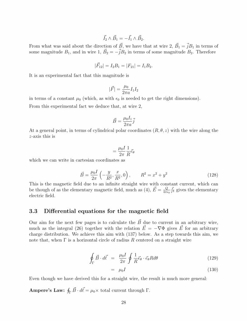
Our aim for the next few pages is to calculate the ~B due to current in an arbitrary wire,much as the integral (26) together with the relation ~E = −∇Φ gives ~E for an arbitrarycharge distribution. We achieve this aim with (137) below. As a step towards this aim, wenote that, when Γ is a horizontal circle of radius R centered on a straight wire

∮Γ

~B · d~̀ =µ0I

2π

∮1

R~eθ · ~eθRdθ (129)

= µ0I (130)

Even though we have derived this for a straight wire, the result is much more general:

Ampere’s Law:∮

Γ~B · d~̀= µ0× total current through Γ.

28

Γ

I

Compare ampere’s law to Gauss Law in the first form we had.

For a current density instead of a wire, we obtain an integral version of Ampere’s Law:

∮Γ

~B · d~̀ = µ0

∫Σ

~J · dS Σ spans Γ

=

∫Σ

∇∧ ~B · dS by Stoke’s theorem

and for this to be true for all Σ we obtain the differential version of Ampere’s law:

∇∧ ~B = µ0~J (131)

(recall that ∇ · ~J = 0 from charge conservation and time independence, and we need this for(131) to make sense). This equation is supplemented by

∇ · ~B = 0 (132)

Which can be explicitly checked for the straight wire, from (128). Equation (132) is to be

contrasted with (23): ∇ · ~E = 1ε0ρ. Thus we interpret (132) as saying ”there are no magnetic

charges”.

The magnetic potential

It follows from (17) that, in a simply-connected region, there exists a function Φ such that~E = −∇Φ. It is a less familiar fact that

Claim: if ∇ · ~B = 0 in a suitable region, then there exists in that region a vector field ~Asuch that

~B = ∇∧ ~A

.

29

~A is the magnetic potential (also called vector potential, in which case Φ is called the scalarpotential).

Note that a change ~A → ~A +∇ζ, for any scalar function ζ, leaves ~B unchanged. We mayexploit this freedom to impose another condition, namely

∇ · ~A = 0

for suppose F = ∇· ~A 6= 0 and change ~A→ ~A+∇· ζ, then this would change F → F +∇2ζ;now, choose ζ such that ∇2ζ = −F , so that now ∇ · ~A = 0.

Equation (131) can be turned into an equation for ~A as follows:

∇∧ ~B = ∇∧ (∇∧ ~A) = ∇(∇ · A)−∇2 ~A

= µ0~J (133)

with the choice ∇ · ~A = 0, then we have

∇2 ~A = −µ0~J (134)

Remember that this is true for the particular choice ∇ · ~A = 0. This has the vector form ofthe Poisson’s equation, and we’ve solved Poisson’s equation before: recall (26) and comparewith (24). So we solve (134) by

~A(~r ) =µ0

4π

∫ ~J(~r ′)

|~r − ~r ′|dV ′

This is for a volume distribution of current. If we have just a line current ~J = I~t, where I isconstant and ~t is the tangent (of unit length) to a curve L (where the curve L is the ”wire”),then instead

~A =µ0I

4π

∫L

~td`

|~r − ~r ′(`)|

t

I

30

where ` parametrizes where we are along the wire.

From the vector potential ~A we can calculate ~B. For a volume distribution

~B(~r) = ∇∧ ~A =µ0

4π∇∧

∫ ~J(~r ′)

|~r − ~r ′|dV ′ (135)

=µ0

4π

∫ ~J(~r ′) ∧ (~r − ~r ′)|~r − ~r ′|3

dV ′ (136)

while for a line distribution/wire

~B(~r) = ∇∧ ~A =µ0I

4π

∫L

~t ∧ (~r − ~r ′)|~r − ~r ′|3

d`

or

B(~r) =µ0I

4π

∫L

d~̀∧ (~r − ~r ′)|~r − ~r ′|3

(137)

Where d~̀ = d`~t. This is now ~B at all points of space due to an arbitrary wire, and sogeneralizes (128). We can use it to obtain an expression for the force between two arbitrarywires, by chopping the second wire into elementary pieces.

P1

P2

r

I 1I 2

At P2 on wire 2

d~F = I2d~̀2 ∧ ~B1

so

~F =

∫I2d~̀2 ∧ ~B1

=µ0I1I2

4π

∫∫d~̀2 ∧ (d~̀1 ∧ (~r2 − ~r1))

|~r2 − ~r1|3(138)

where ~r1 = ~r1(`1) belongs to wire 1 and ~r2 = r2(`2) belongs to wire 2. This is the Biot-SavartLaw for the force between two arbitrary current-carrying wires (more precisely, the force onwire 2 done by wire 1). Its interest is largely theoretical, as it is rather hard to use.

31

3.4 The story so far

We’ve studied time-independent electricity (or electrostatics) and time-independent mag-netism (or magnetostatics), and found these to be governed by the following system ofequations

∇ · ~E =1

ε0ρ ∇ · ~B = 0

∇∧ ~E = 0 ∇∧ ~B = µ0~J (139)

with the understanding that

∂ ~E

∂t= 0 =

∂ ~B

∂t=∂ ~J

∂t=∂ρ

∂t.

The electric and magnetic field strengths themselves can be defined from the force laws (7)and (127), which we combine as follows: a particle with charge Q moving with velocity ~v in

a combination of an electric field ~E and a magnetic field ~B is subject to the force given by

~F = Q( ~E + ~v ∧ ~B).

In addition we have one equation which we expect to be valid also in the time-dependentcase, namely the charge conservation equation

∂ρ

∂t+∇ · ~J = 0. (140)

The problem now is how to extend all these equations to the time-dependent case, i.e. howto put back the terms that are zero in the time-independent case. This will be the subjectof the next part of this course.

32

4 Time dependent electromagnetism

4.1 Maxwell equations

Experimental evidence suggests two qualitative facts:

• A time-varying ~B produces an ~E.

• A time-varying ~E produces a ~B.

This experimental evidence can be summarized quantitatively in the following two integrallaws:

∮Γ

~E · d~̀ = − d

dt

∫Σ

~B · dS Faraday’s law of induction (141)

∮Γ

~B · d~̀ =

∫Σ

µ0~J · d~S +

∫Σ

ε0µ0∂ ~E

∂t· d~S (142)

Where Σ spans Γ. Apply Stoke’s theorem to both to obtain

∫Σ

(∇∧ ~E +

∂ ~B

∂t

)· d~S = 0 (143)

∫Σ

(∇∧ ~B − µ0

~J − ε0µ0∂ ~E

∂t

)· d~S = 0 (144)

and if these hold for all Σ we obtain the

Maxwell equations:

∇∧ ~E +∂ ~B

∂t= 0; ∇∧ ~B = µ0

~J +1

c2

∂ ~E

∂t

∇ · ~B = 0, ∇ · ~E =1

ε0ρ (145)

with c2 = 1ε0µ0

.

These are the Maxwell’s equations, the basic equations of the new theory of electromagnetism,in which electricity and magnetism are merged.

Note that

• Two of the equations always have zero on the right; the other two contain the sourcesρ and ~J .

33

• If all time-derivatives are set to zero, we recover the equations of the previous section.

• The system obtained by setting ρ and ~J to zero is called source-free Maxwell equations.

• Regarding ρ and ~J as given, there are eight equations for six unknowns, so there shouldbe a consistency condition.

To see what the consistency condition is, calculate:

∂ρ

∂t= ε0

∂

∂t(∇ · ~E) = ε0∇ ·

(∂ ~E

∂t

)

=1

µ0

∇ ·(∇∧ ~B − µ0

~J)

= −∇ · ~J

which we recognize as the charge conservation equation. From this point of view the chargeconservation equation is a consistency condition for the Maxwell’s equations. As an exercise,show that there is a second consistency condition but that it is automatically satisfied.

Energy of the Electromagnetic Field

There is a deductive way to approach this question, but we shall rely on intuition andguesswork. We want an energy density (energy-per-unit-volume) which is something like”1/2m~v · ~v”.

After playing around with Maxwell equations for a while, we are lead to consider

E =1

2ε0| ~E|2 +

1

2µ0

| ~B|2 (146)

Then, using the Maxwell equations, we calculate

∂E∂t

= ε0 ~E ·∂ ~E

∂t+

1

µ0

~B · ∂~B

∂t

=1

µ0

~E ·(∇∧ ~B − µ0

~J)− 1

µ0

~B · ∇ ∧ ~E

= −∇ ·(

1

µ0

~E ∧ ~B

)− ~E · ~J

For the source-free case, we set ~J = 0 so that the last term vanishes. Then, this has theform of a conservation equations

∂E∂t

+∇ · ~P = 0 (147)

34

Remember that E is the energy density. ~P ≡ 1µ0~E ∧ ~B is called the Poynting vector and has

the interpretation of the rate of energy flow, or momentum density.

If we now reinstate the sources, this equation has a name:

Poynting’s theorem

∂E∂t

= −∇ · ~P − ~E · ~J

We integrate Poynting’s theorem over a volume V with surface S to obtain an energy balanceequation:

d

dt

∫V

EdV = −∫S

~P · d~S −∫V

~E · ~JdV

(1) (2) (3)

where each term has the following interpretation:

1. Rate of increase of electromagnetic energy.

2. Rate of energy flow into V .

3. Rate of work done by the field on sources.

To justify the interpretation of (3), consider a single charge. Remember that work is the

product of force and displacement W = ~F ·d~̀, so the rate of work is dWdt

= ~F ·~v. For a single

charge ~F = q ~E and q~v is by definition the current ~j, so that dWdt

= ~E · ~j. This satisfactoryinterpretation of the third term reinforces the interpretation of E as energy density.

4.2 Electromagnetic potentials

The introduction of potentials in the time-dependent case is similar to that in the time-independent case. Assume we are interested in a suitable (simply-connected, etc) region ofspace, then the Maxwell equations imply, first:

∇ · ~B = 0⇒ ∃ ~A such that ~B = ∇∧ ~A;

next ∂ ~B∂t

= ∇∧ ∂ ~A∂t

, so that

∇∧ ~E +∂ ~B

∂t= ∇∧

(~E +

∂ ~A

∂t

)= 0,

whence

35

∃Φ such that ~E +∂ ~A

∂t= −∇Φ

i.e.

~B = ∇∧ ~A (148)

~E = −∇Φ− ∂ ~A

∂t(149)

As before, we have the freedom to modify ~A and Φ slightly without changing the electricand magnetic fields. This freedom has the name of gauge transformation:

~A→ ~A+∇ζ (150)

Φ→ Φ− ∂ζ

∂t(151)

This gauge transformation and can be exploited, as before, to simplify potentials.

Plugging the expression for the fields in terms of their potentials into the Maxwell equationswe obtain

∇2Φ +∂

∂t∇ · ~A = − 1

ε0ρ (152)

∇2 ~A− 1

c2

∂2 ~A

∂t2−∇

(∇ · ~A+

1

c2

∂Φ

∂t

)= −µ0

~J (153)

This is a nice set of equations for the potentials, but they are coupled. You can show thatthe gauge transformations can be used in order to choose potentials such that

∇ · ~A+1

c2

∂Φ

∂t= 0 (154)

For this particular choice we obtain

∇2Φ− 1

c2

∂2Φ

∂t2= − 1

ε0ρ (155)

∇2 ~A− 1

c2

∂2 ~A

∂t2= −µ0

~J (156)

These equations, supplemented with our gauge choice (154) are completely equivalent toMaxwell equations. In order to solve these equations, and give the time-dependent of (26)and (137), we need to introduce a new concept.

36

4.3 Time-dependent Green’s functions

The inhomogeneous wave equations found in the previous section have the structure

∇2ψ − 1

c2

∂2ψ

∂t2= −4πf(~r, t) (157)

where c is the velocity and f(~r, t) is a known source term. In order to solve this equation,it is convenient to find the corresponding Green’s function, as we did for electrostatics. Bydefinition

∇2G(~r, t;~r ′, t′)− 1

c2

∂2

∂t2G(~r, t;~r ′, t′) = −4πδ(~r − ~r ′)δ(t− t′) (158)

We will focus on situations without boundaries and choose our Green’s function to be afunction of the differences ~r − ~r ′ and t − t′. As we have seen, the delta functions have thefollowing integral representation

δ(~r − ~r ′)δ(t− t′) =1

(2π)4

∫ ∞−∞

d3k

∫ ∞−∞

dωei~k·(~r−~r ′)e−iω(t−t′) (159)

Hence it is natural to represent the Green’s function as

G(~r, t;~r ′, t′) =

∫ ∞−∞

d3k

∫ ∞−∞

dωg(~k, ω)ei~k·(~r−~r ′)e−iω(t−t′) (160)

Acting on both sides of (160) with the wave operator

∇2 − 1

c2

∂2

∂t2(161)

and comparing with the delta function representation (159) we obtain

g(~k, ω) =1

4π3

1

k2 − ω2

c2

(162)

The manipulations we did here are exactly the same we did to arrive to (90), however, thereis a crucial difference: as we plug back (162) into (160) and try to do the integral over ω, wefind two poles along the real line, at

ω = ck, ω = −ck (163)

Note that this is due to the minus sign in front of the second time derivative in the waveequation. In order to compute (160) we need to give a prescription on how to treat thesepoles. In similar situations in physics one adds a small imaginary part and moves the polesa little above or below the real axis. In order to know which one of the choices is the correctone, we turn into physical considerations.

37

What is the meaning of G(~r, t;~r ′, t′)? it represents the wave caused by a disturbance at~r = ~r ′, t = t′. Hence, for t < t′ we demand G(~r, t;~r ′, t′) to vanish identically (since thedisturbance didn’t happen yet!)

G(~r, t;~r ′, t′) = 0, for t < t′ (164)

Looking at (160) we see that for t < t′ we can compute the integral over ω by closing thecontour at infinity from above. Indeed, for t− t′ < 0 the contribution from the circle abovevanishes exponentially. The correct prescription for the poles is then to push them slightlybelow the real axis:

ω = ck − iε, ω = −ck − iε (165)

so that the integral over ω vanishes for the case t < t′. See figure

ω-plane

t<t'

t>t'

-c k - i ε c k - i ε

C

Now, lets turn out to the more interesting situation t > t′. In this case we can compute theintegral over ω by closing the contour from below. By residue theorem we obtain∫

Cdω

1

k2 − (ω+iε)2

c2

e−iω(t−t′) = 2πcsin (ck(t− t′))

k(166)

Hence

G(~r, t;~r ′, t′) =c

2π2

∫ ∞−∞

d3kei~k·(~r−~r ′) sin (ck(t− t′))

k(167)

=2c

π|~r − ~r ′|

∫ ∞0

dk sin(k|~r − ~r ′|) sin (ck(t− t′)) (168)

=c

π|~r − ~r ′|

∫ ∞−∞

dk sin(k|~r − ~r ′|) sin (ck(t− t′)) (169)

where in the second line we have used spherical coordinates for ~k and integrated over theangular variables. In the third line we have simply extended the integration region to thewhole real line. Then, using the exponential form of the trigonometric functions we end up

38

with the integral representation for the delta function (73). One delta is identically zero ast− t′ > 0, while the other one gives

G(~r, t;~r ′, t′) =δ(t′ + |~r−~r ′|

c− t)

|~r − ~r ′|(170)

We see that the Green’s function vanishes identically outside the sphere |~r − ~r ′| = c(t− t′).This result fits perfectly with the interpretation of G(~r, t;~r ′, t′) as a wave that originatesfrom the perturbation at ~r = ~r ′ and t = t′ and then expands spherically at velocity c. ThisGreen’s function is also called the retarded Green’s function: the effect observed at the point~r at time t is due to the perturbation originated at a retarded time t′ = t − |~r−~r

′|c

. Hence,the final solution to the inhomogeneous wave equation (157) in the absence of boundaries is

ψ(~r, t) =

∫ δ(t′ + |~r−~r ′|

c− t)

|~r − ~r ′|f(~r ′, t′)dV ′dt′ =

∫f(~r ′, t− |~r−~r

′|c

)

|~r − ~r ′|dV ′ (171)

This allows to write the solution for the scalar and vector potential wave equations (155) inthe absence of boundaries for arbitrary charge and current distributions.

φ(~r, t) =1

4πε0

∫ρ(~r ′, t− |~r−~r

′|c

)

|~r − ~r ′|dV ′ (172)

~A(~r, t) =µ0

4π

∫ ~J(~r ′, t− |~r−~r′|

c)

|~r − ~r ′|dV ′ (173)

We leave it as an exercise to show that this solution indeed satisfies the gauge (154).

4.4 Maxwell equations in macroscopic/dielectric media

Consider the basic equations of electrostatics

∇∧ ~E = 0, ∇ · ~E =1

ε0ρ (174)

writing them down for a real situation would require a precise knowledge of the chargedensity at all points of space. Except some ideal situations (e.g. a collection of charges inthe vacuum) such a knowledge is impossible. For instance, if we are studying electrostatics inwater, on a cubic centimeter there would be billions of atoms with their electrons and protons(which are furthermore vibrating!) and they would have to be accounted for. Luckily onecan write an effective set of equations which describes electrostatics in macroscopic media.For the simplest case of media they amount to simply replacing the value of ε0 valid for hevacuum by ε, which characterizes the medium:

39

∇∧ ~E = 0, ∇ · (ε ~E) = ρ (175)

where now the medium itself does not contribute to the charge density. The ratio ε/ε0 iscalled the dielectric constant of the medium, such that the dielectric constant of the vacuumis one. For other materials the dielectric constant is always larger than one. For instance,the dielectric constant of air is very close to 1 (about 1.0005), while the dielectric constantof water is about 2.

These effective equations can be understood as follows. Usually a macroscopic mediumcontains dipoles 6. In the absence of an electric field these dipoles are randomly aligned. Aswe turn an electric field, however, these dipoles align, producing themselves a net electricfield. This alignment (and the field the dipoles produce) is proportional to the applied electricfield, effectively changing the value of ε and giving (175). For most examples studied in thislectures ε will be just a constant, for which the effective equations exactly coincide with theequations on the vacuum, upon replacing ε0 → ε. An exception will be problems where aplane separates two regions with different values of ε. In this case, by applying Gauss law,we can see that as we cross the boundary(

ε1 ~E1 − ε2 ~E2

)· ~n = 0 (176)

On the other hand, by applying Stokes theorem we obtain(~E1 − ~E2

)∧ ~n = 0 (177)

where ~n is the normal to the boundary. Hence, as we cross the boundary, we must imposecontinuity for the normal component of ε ~E and the tangential components of ~E.

A similar description can be given for the equations of magnetostatics, and the effectiveequations take the form

∇∧ 1

µ~B = ~J, ∇ · ~B = 0 (178)

The ratio µ/µ0 is called permeability of the medium. It is one for the vacuum, extremelyclose to one for air and slightly less than one for water. As before, as we cross the boundarybetween two regions with different magnetic permeabilities we obtain(

1

µ1

~B1 −1

µ2

~B2

)∧ ~n = 0,

(~B1 − ~B2

)· ~n = 0 (179)

Hence, as we cross the boundary the tangential components of 1µ~B and the normal com-

ponents of ~B are continuous. Finally, the effective Maxwell equations in the presence of amedium with constant ε, µ take the form

6You can think of a dipole as two opposite charges very close to each other. The dipole is said to bealigned in the direction of separation of the charges.

40

∇∧ ~E +∂ ~B

∂t= 0; ∇∧ ~B = µ~J + µε

∂ ~E

∂t

∇ · ~B = 0, ∇ · ~E =1

ερ (180)

41

5 Electromagnetic waves

In this section we will study the source-free Maxwell equations and show that they admitwave solutions. We will then study many properties of these solutions.

5.1 Plane waves

We start from the Source-free Maxwell equations:

∇ · ~B = 0, ∇ · ~E = 0 (181)

∇∧ ~E + ∂ ~B∂t

= 0, ∇∧ ~B − 1c2∂ ~E∂t

= 0

we would like to decouple the equations for ~E and ~B. Calculate:

∇∧ (∇∧ ~E) = ∇(∇ · ~E)−∇2 ~E = −∇2 ~E

= −∇ ∧ ∂~B

∂t= − ∂

∂t(∇∧ ~B) = − 1

c2

∂2 ~E

∂t2

so that

∇2 ~E − 1

c2

∂2 ~E

∂t2= 0 (182)

which is the wave-equation with c = (ε0µ0)−1/2 as the wave speed. Similarly (exercise)

∇2 ~B − 1

c2

∂2 ~B

∂t2= 0 (183)

We want to solve these wave equations, so think first about a scalar version

∇2F − 1

c2

∂2F

∂t2=∂2F

∂x2+∂2F

∂y2+∂2F

∂z2− 1

c2

∂2F

∂t2= 0 (184)

and try F = f(~k · ~r − ωt) with constant ω and ~r. Then

∂F

∂t= −ωf ′, ∇F = ~kf ′

∂2F

∂t2= ω2f ′′, ∇2F = k2f ′′

Hence, F = f(~k ·~r−ωt) is a solution for any (twice-differentiable) f provided k2 = ω2

c2. Note

that F is constant on surfaces

42

~k · ~r − ωt = const

at a fixed t this is the equation of a plane, so these solutions are called plane waves. As timegoes forward, the wavefront propagates in the direction of ~k. If f is of the form

f(~k · ~r − ωt) ∼ ei(~k·~r−ωt) (185)

then they are called harmonic waves or or monochromatic plane waves with a single frequencyω and wave number k. Note that both the real part and imaginary part of the exponentialabove will be solutions of the wave equation.

After this discussion, we try

~E = ~eE0 ei(~k·~r−ωt) (186)

~B = ~bB0 ei(~k·~r−ωt),

With the understanding that the electric and magnetic fields are the real part of the solutions.Here ~e and ~b are unit vectors characterizing the direction of the fields and E0 and B0 areconstants. Plugging these expressions into ∇ · ~B = 0, ∇ · ~E = 0 we obtain

~e · ~k = 0, ~b · ~k = 0 (187)

This means that both ~E and ~B are perpendicular to the direction of propagation of the wave.Such a wave is called transverse wave. The rest of the Maxwell equations imply

(~k ∧ ~e)E0 − ω~bB0 = 0 (188)

(~k ∧~b)B0 +ω

c2~eE0 = 0 (189)

This system implies the expected relation k2 = ω2

c2, shows that ~e and ~b are perpendicular to

each other and fixes the relative magnitudes:

B0 =1

cE0, ~b =

1

k~k ∧ ~e → ~e ·~b = 0 (190)

These are transverse waves (unlike e.g. sound). The waves travel in the direction of ~k, while~E and ~B lie in wave fronts, transverse to the direction of propagation, and are orthogonalto each other, see figure below.

K

E, e i

B, b i

direction of wave

43

5.2 Polarization

Let us discuss the phenomenon of polarization. To simplify the expressions, take ~k in thez-direction, ~k · ~r = kz. Look in the plane z = 0 so that the argument of the wave solutionsis simply ωt. Taking linear combinations of the solutions above we can write

~E = ~e1 cosωt+ ~e2 sinωt (191)

~B =1

ω~k ∧ ~e1 cosωt+

1

ω~k ∧ ~e2 sinωt (192)

where ~e1 and ~e2 are two a priori independent vectors. To discuss the phenomenon of polari-sation, we distinguish some particular cases:

(i) ~e1, ~e2 proportional, say to ~i, then

~E = E~i cos(ωt+ δ) (193)

~B =1

cE~j cos(ωt+ δ) (194)

for some constant δ;

x

y

c B

E

a wave like this is said to be lineary polarised; ~E and ~B oscillate parallel to two fixedorthogonal directions.

(ii) ~e1, ~e2 orthogonal, of equal length, e.g. ~e1 = E~i,~e2 = E~j, then

~E = E(~i cosωt+~j sinωt) (195)

~B =E

c(−~i sinωt+~j cosωt); (196)

a wave like this is said to be circularly polarised; ~E and ~B rotate at a constant rate aboutthe direction of propagation.

44

ω t

x

y

EcB

The direction is anti-clockwise and the wave is left circularly polarized if ~e1 ∧ ~e2 · ~k > 0, andthe rotation is clockwise and the wave is right circularly polarized if ~e1 ∧ ~e2 · ~k < 0.

(iii) the general case can be regarded as a combination of waves with different polarizations.

5.3 Reflection and refraction of electromagnetic waves

If you have ever been to a swimming pool you know about the funny properties of light asit crosses the boundary between air and water. The basic laws of optics regarding reflectionand refraction of light can be summarized as follows:

1.- The angle of reflection equals the angle of incidence.

2.- Each material has an index of refraction n and the angles of incidence α andrefraction α′ satisfy

n sinα = n′ sinα′

For air the index of refraction is almost exactly 1, while for water is about 1.3.

Let us discuss how the laws of reflection and refraction of light at a plane surface betweentwo media of different dielectric properties (for instance air and water) can be deduced fromthe Maxwell equations. Consider a plane surface located at z = 0 separating two media withεµ and ε′µ′, and consider an incident wave along ~k which ”splits” into a refracted wave along~k′ and a reflected wave along ~k′′, see figure:

45

ε'μ'

ε μ

k

k'

k''

α α''

α'

z

For z > 0 the solution corresponds to the incident plus the reflected waves

~E = ~E0ei(~k.~r−ωt) + ~E ′′0e

i(~k′′.~r−ωt) (197)

~B =1

ω

(~k ∧ ~E0e

i(~k.~r−ωt) + ~k′′ ∧ ~E ′′0ei(~k′′.~r−ωt)

)(198)

while for z < 0 the solution corresponds to the refracted wave

~E = ~E ′0ei(~k′.~r−ωt) (199)

~B =1

ω~k′ ∧ ~E0e

i(~k′.~r−ωt) (200)

Here ~E0 and ~k are arbitrary (since we can send in any wave we want) and we need to fix~E ′0,

~E ′′0 and ~k′, ~k′′ in terms of these, by requiring the correct boundary conditions at z = 0.The wave numbers satisfy

k = k′′ =ω

v, k′ =

ω

v′(201)

where v and v′ are the velocities of the waves in the two media, related to the properties ofthe medium by

v =1√ε µ

=

√ε0µ0

ε µc, v′ =

1√ε′µ′

=

√ε0µ0

ε′µ′c (202)

Whatever conditions we have at z = 0 the spacial variation of the three waves, as we movealong the z = 0 plane, should be the same (as they should work for all x, y) hence

~k.~r |z=0 = ~k′.~r |z=0 = ~k′′.~r |z=0 (203)

46

independent of the nature of the boundary conditions. In particular the three wave vectorsshould lie on a plane, let’s say (x, z), and their component along the x direction shouldcoincide, namely

k sinα = k′ sinα′ = k′′ sinα′′ (204)

This implies

α = α′′,1

vsinα =

1

v′sinα′ (205)

These are the two basic laws of optics! the refraction index is usually defined as n =√

εµε0µ0

.

We haven’t yet imposed the precise boundary conditions at z = 0. As we cross the boundary,remember that the normal components of ε ~E and ~B are continuous and the tangentialcomponents of ~E and µ−1 ~B:

(ε( ~E0 + ~E ′′0 )− ε′ ~E ′0

)· ~n = 0 (206)(

~k ∧ ~E0 + ~k′′ ∧ ~E ′′0 − ~k′ ∧ ~E ′0)· ~n = 0 (207)(

~E0 + ~E ′′0 − ~E ′0

)∧ ~n = 0 (208)(

1

µ

(~k ∧ ~E0 + ~k′′ ∧ ~E ′′0

)− 1

µ′~k′ ∧ ~E ′0

)∧ ~n = 0 (209)

These equations can be used to compute the magnitude of the reflected and refracted fieldsin terms of the incident one. For instance, assume for simplicity that the electric field islinearly polarized along the direction perpendicular to the incidence plane (the plane formed

by ~k and ~n), namely ~E0, ~E′0,~E ′′0 are all along the y direction (going out from the picture). In

this case, (206) imply

E0 + E ′′0 − E ′0 = 0 (210)√ε

µ(E0 − E ′′0 ) cosα−

√ε′

µ′E ′0 cosα′ = 0 (211)

Assuming µ = µ′ (which is almost true for instance for light from air reflected on water) andusing (205) we obtain

E ′0 =2 cosα sinα′

sin(α + α′)E0 (212)

E ′′0 = −sin(α− α′)sin(α + α′)

E0 (213)

The correct description of light and the laws of optics was one of the biggest triumphs ofelectromagnetism!

47

6 Epilogue: Electromagnetism and Special Relativity

In order to apply the second law of Newton ~F = m~a, compute the path of particles undercentral forces, etc, you need to choose a system of reference. However, provided the systemis inertial you can choose any system you want. In particular, your description and thedescription of your classmate should be equivalent if your two systems are moving withconstant velocity with respect to each other (all inertial frames move with constant velocitywith respect to each other). This is also true for other laws of Physics, and so we can makethe following postulate:

1.- The laws of Physics are the same in all inertial frames of reference.

Should electromagnetism be any different? Imagine it is not. More precisely, if I, in my nicestationary lab, measure forces between wires and charges, I will find out they are describedby the electromagnetism equations with some specific ε0 and µ0. Now, if your lab is moving(at a constant velocity) and you repeat the same experiments, you should find the sameresults, with the same ε0 and µ0. In particular, if we both produce electromagnetic waves,both of us will see that these waves move at speed c = 1√

ε0µ0. This leads to the second

postulate:

2.- The speed of light c has the same value in all inertial frames.

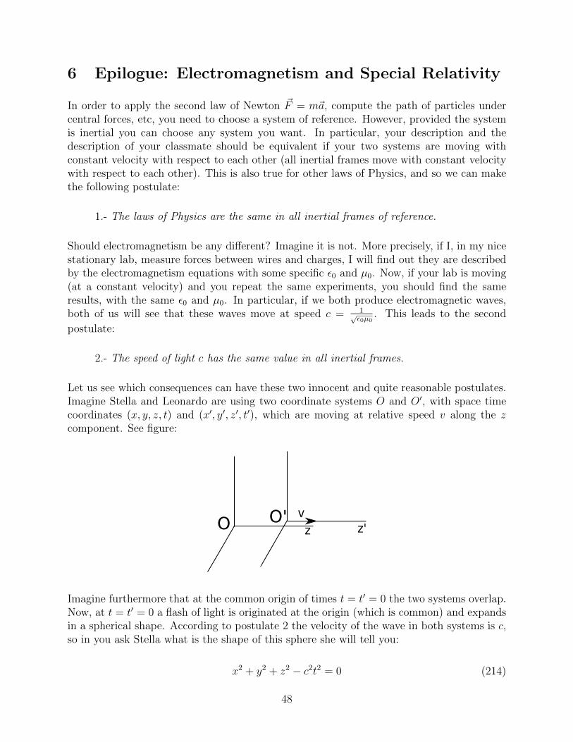
Let us see which consequences can have these two innocent and quite reasonable postulates.Imagine Stella and Leonardo are using two coordinate systems O and O′, with space timecoordinates (x, y, z, t) and (x′, y′, z′, t′), which are moving at relative speed v along the zcomponent. See figure:

O zO'

z'

v

Imagine furthermore that at the common origin of times t = t′ = 0 the two systems overlap.Now, at t = t′ = 0 a flash of light is originated at the origin (which is common) and expandsin a spherical shape. According to postulate 2 the velocity of the wave in both systems is c,so in you ask Stella what is the shape of this sphere she will tell you:

x2 + y2 + z2 − c2t2 = 0 (214)

48

If instead you ask Leonardo what is the shape of the sphere in his system he will tell you:

x′2 + y′2 + z′2 − c2t′2 = 0 (215)

There should be some way now to translate between the two systems. Galileo will tell youthat this is easy, indeed, looking at the pictures:

x′ = x (216)

y′ = y (217)

z′ = z − vt (218)

t′ = t (219)

This is called a Galilean transformation, is the transformation you would use, and has beenused for centuries, but it does not agree with (214) and (215)!! If you assume that therelations between the set of variables is linear and you insist on consistency with (214) and(215) you find:

x′ = x, y′ = y (220)

z′ =z − vt√1− v2

c2

(221)

t′ =t− v

c2z√

1− v2

c2

(222)

These are called the Lorentz transformations and you can see that they reduce to Galileantransformations for velocities much smaller than c. One of the most surprising aspects ofthese transformations is that the time intervals between the two systems are not the same!and Stella (t) will look at the watch of Leonardo (t’) and think that Leonardo’s watch isgoing slower!

Lorentz actually found these transformations by studying the Maxwell equations, and realiz-ing that they were not invariant under Galilean transformations. Einstein proved that thesetransformations actually followed from his postulates 1 and 2 (which however have widervalidity). In this way special relativity was born.

49