electromechanical motion systems - design and...

Frederick G. Moritz

Electromechanical Motion Systems -Design and Simulation

ELECTROMECHANICALMOTION SYSTEMS

ELECTROMECHANICALMOTION SYSTEMSDESIGN AND SIMULATION

Frederick G. MoritzFM Systems, Ohio, USA

This edition first published 2014C© 2014 John Wiley & Sons, Ltd

Registered officeJohn Wiley & Sons Ltd, The Atrium, Southern Gate, Chichester, West Sussex, PO19 8SQ, United Kingdom

For details of our global editorial offices, for customer services and for information about how to apply forpermission to reuse the copyright material in this book please see our website at www.wiley.com.

The right of the author to be identified as the author of this work has been asserted in accordance with the Copyright,Designs and Patents Act 1988.

All rights reserved. No part of this publication may be reproduced, stored in a retrieval system, or transmitted, in anyform or by any means, electronic, mechanical, photocopying, recording or otherwise, except as permitted by the UKCopyright, Designs and Patents Act 1988, without the prior permission of the publisher.

Wiley also publishes its books in a variety of electronic formats. Some content that appears in print may not beavailable in electronic books.

Designations used by companies to distinguish their products are often claimed as trademarks. All brand names andproduct names used in this book are trade names, service marks, trademarks or registered trademarks of theirrespective owners. The publisher is not associated with any product or vendor mentioned in this book.

Limit of Liability/Disclaimer of Warranty: While the publisher and author have used their best efforts in preparingthis book, they make no representations or warranties with respect to the accuracy or completeness of the contents ofthis book and specifically disclaim any implied warranties of merchantability or fitness for a particular purpose. It issold on the understanding that the publisher is not engaged in rendering professional services and neither thepublisher nor the author shall be liable for damages arising herefrom. If professional advice or other expertassistance is required, the services of a competent professional should be sought.

MATLAB R© is a trademark of The MathWorks, Inc. and is used with permission. The MathWorks does not warrantthe accuracy of the text or exercises in this book. This book’s use or discussion of MATLAB R© software or relatedproducts does not constitute endorsement or sponsorship by The MathWorks of a particular pedagogical approach orparticular use of the MATLAB R© software.

Library of Congress Cataloging-in-Publication Data

Moritz, Frederick G.Electromechanical motion systems : design and simulation / Frederick G. Moritz.

pages cmIncludes bibliographical references and index.ISBN 978-1-119-99274-5 (hardback)

1. Servomechanisms. 2. Robotics. I. Title.TJ214.M6576 2013629.8′323–dc23

2013023514

A catalogue record for this book is available from the British Library.

ISBN: 9781119992745

Typeset in 10/12pt Times by Aptara Inc., New Delhi, India

1 2014

http://www.wiley.com

To my wife,

Louise,

For her enthusiastic support and encouragement

Contents

Acknowledgements xiii

1 Introduction 11.1 Targeted Readership 21.2 Motion System History 21.3 Suggested Library for Motion System Design 5

Reference 6

2 Control Theory Overview 72.1 Classic Differential/Integral Equation Approach 72.2 LaPlace Transform-the S Domain 102.3 The Transfer Function 132.4 Open versus Closed Loop Control 15

2.4.1 Transient and Frequency Response 182.5 Stability 222.6 Basic Mechanical and Electrical Systems 23

2.6.1 Equations and Constants 232.6.2 Power Test 262.6.3 Retardation Test 26

2.7 Sampled Data Systems/Digital Control 282.7.1 Sampling 282.7.2 Quantization 302.7.3 Computational Delay 302.7.4 System Analysis 31References 34

3 System Components 353.1 Motors and Amplifiers 35

3.1.1 Review of Motor Theory 363.1.2 The Brush Motor 373.1.3 The “H” Drive PWM Amplifier 463.1.4 The Brushless Motor 483.1.5 Speed/Torque Curves 573.1.6 Thermal Effects 59

viii Contents

3.1.7 Motor Constant 723.1.8 Linear Motor 743.1.9 Stepper Motors 783.1.10 Induction Motors 97

3.2 Gearheads 1073.2.1 Spur Gearhead 1073.2.2 Planetary Gearhead 1093.2.3 Hybrid Gearhead 1103.2.4 Worm Gearhead 1103.2.5 Harmonic Gearhead 1103.2.6 Gearhead Sizing – Continuous Operation 1113.2.7 Gearhead Sizing – Intermittent Operation 1123.2.8 Axial and Radial Load 1143.2.9 Backlash and Stiffness 1143.2.10 Temperature/Thermal Resistance 1163.2.11 Planetary/Spur Gearhead Comparison 118

3.3 Leadscrews and Ballscrews 1193.3.1 Leadscrew Specifications 1203.3.2 Ball Screw Specifications 1203.3.3 Critical Speed 1213.3.4 Column Strength 1223.3.5 Starts, Pitch, Lead 1243.3.6 Encoder/Lead 1253.3.7 Accuracy 1253.3.8 Backdrive – Self-Locking 1253.3.9 Assemblies 125

3.4 Belt and Pulley 1263.4.1 Belt 1283.4.2 Guidance/Alignment 1283.4.3 Belt and Pulley versus Ball Screw 129

3.5 Rack and Pinion 1293.5.1 Design Highlights 1303.5.2 Backlash 1303.5.3 Dynamics 131

3.6 Clutches and Brakes 1323.6.1 Clutch/Brake Types 1323.6.2 Velocity Rating 1343.6.3 Torque Rating 1343.6.4 Duty Cycle/Temperature Limits 1353.6.5 Timing 1373.6.6 Control 1393.6.7 Brake/System Timing 1403.6.8 Soft Start/Stop 140

3.7 Servo Couplings 1403.7.1 Inertia 1413.7.2 Velocity 141

Contents ix

3.7.3 Torque 1413.7.4 Compliance 1413.7.5 Misalignment 1433.7.6 Coupling Types 143

3.8 Feedback Devices 1463.8.1 Optical Encoders 1463.8.2 Magnetic Encoders 1523.8.3 Capacitive Encoders 1533.8.4 Magnetostrictive/Acoustic Encoders 1533.8.5 Resolvers 1533.8.6 Inductosyn 1573.8.7 Potentiometer 1583.8.8 Tachometers 162References 164Additional Readings 165

4 System Design 1674.1 Position, Velocity, Acceleration, Jerk, Resolution,

Accuracy, Repeatability 1674.1.1 Position 1674.1.2 Velocity 1694.1.3 Acceleration 1704.1.4 Jerk 170

4.2 Three Basic Loops – Current/Voltage, Velocity, Position 1704.2.1 Current/Voltage Loop 1714.2.2 Velocity Loop 1774.2.3 Position Loop 181

4.3 The Velocity Profile 1824.3.1 Preface 1824.3.2 Incremental Motion 1834.3.3 Constant Motion 1924.3.4 Profile Simulation 194

4.4 Feed Forward 1954.5 Inertia 200

4.5.1 Preface 2004.5.2 Motor Selection 2024.5.3 Reflected Inertia – Gearhead 2034.5.4 Torque versus Optimum Ratio – Gearhead 2044.5.5 Power versus Optimum Ratio – Gearhead 2044.5.6 Optimal Conditions 208

4.6 Shaft Compliance 2104.6.1 Basic Equations 2114.6.2 System Components 2124.6.3 Initial Simulation – Lumped Inertia 2124.6.4 Second Simulation – Inclusion of Shaft Dynamics 212

x Contents

4.6.5 Third Simulation – Compensation 2144.6.6 Coupling Simulation 215

4.7 Compensation 2164.7.1 Routh–Hurwitz 2164.7.2 Nyquist 2174.7.3 Bode 2174.7.4 Root Locus 2184.7.5 Phase Plane 2184.7.6 PID 2184.7.7 Notch Filter 223

4.8 Nonlinear Effects 2244.8.1 Coulomb Friction 2244.8.2 Stiction 2254.8.3 Limit 2264.8.4 Deadband 2264.8.5 Backlash 2284.8.6 Hysteresis 229

4.9 The Eight Basic Building Blocks 2304.9.1 Rotary Motion – Direct Drive 2304.9.2 Rotary Motion – Gearhead Drive 2344.9.3 Rotary Motion – Belt and Pulley Drive 2374.9.4 Linear Motion – Leadscrew/Ballscrew Drive 2394.9.5 Linear Motion – Belt and Pulley Drive 2424.9.6 Linear Motion – Rack and Pinion Drive 2454.9.7 Linear Motion – Roll Feed Drive 2484.9.8 Linear Motion – Linear Motor Drive 251References 253

5 System Examples – Design and Simulation 2555.1 Linear Motor Drive 2555.2 Print Cylinder Control 2575.3 Conveyor System – Clutch/Brake Control 261

5.3.1 Determine Basic Parameters 2615.3.2 Initial Component Selection 2645.3.3 Simulate System 264

5.4 Bang-Bang Servo (Slack Loop System) 2675.5 Wafer Spinner 272

Appendix 275A.1 Brushless Motor Speed/Torque Curves 275

A.1.1 Thermal Resistance 275A.1.2 Core Losses 276

A.2 Inertia Calculation – Excel Program 277A.3 Time Constants versus Viscous Damping Constant 277A.4 Current Drive Review 279A.5 Conversion Factors 285

Contents xi

A.6 Work and Power 286A.6.1 Work (Energy) 286A.6.2 Power 286A.6.3 Horsepower (HP) 286A.6.4 Rotary Power 287

A.7 I2R Losses 287A.7.1 Conventional DC Motor 287A.7.2 Three Phase Brushless DC Motor with Trapezoidal BEMF

and Six Step Drive 288A.7.3 Three Phase Brushless DC Motor with Sine Wave BEMF

and Drive 289A.8 Copper Resistivity 290

Index 291

Acknowledgements

To Roger Mosciatti and Thomas Foley, my partners for over 25 years at MFM Technology;the two most inventive and dedicated engineers it has been my pleasure to know. Our effortsindividually and together led to over 20 US patents and a highly successful manufacturer ofmotion control products and systems.

To Hans Waagen, an engineer who combines an in-depth knowledge of motion control withan ability to concisely analyze and interpret a customers’ product requirements.

To Avi Telyas, founder of the Bayside Motion Group, an entrepreneur who understands andsupports the engineers’ contribution to the success of high tech business ventures.

To Dr. Duane Henselman, University of Maine, who has the ability to combine theory withthe practical requirements of product design and manufacturing.

To Art Shoemake, for supplying many of the illustrations in this book.

To Visual Solutions, Inc., creator of the VisSim simulation software used throughout the book,for their encouragement and support in the creation of the product and system simulationdiagrams.

To my wife Louise and son Peter for their able participation in checking the manuscript andproofs of the complete book.

1Introduction

Having spent the first half of my engineering career in the design of motion control systemsin computer peripheral equipment (digital tape recorders, disc memories and high speed lineprinters) and the second half in the design, manufacture and application of brushless motors,gearheads and slides, I have been both a user and a supplier of the various components usedin high performance servo/control systems.

Time restraints in a typical one or two semester motion control/servo system course requirethat the text and class time devote a majority of their content to topics such as pertinent mathe-matics, LaPlace transform, linear system analysis, closed loop control theory and stabilizationtechniques. Little time can be devoted to a detailed presentation of the system components,which are typically presented in a cursory fashion only as needed to aid in the discussion ofthe system theory.

This book will extend such course work by providing an introduction to the technology ofthe major components that are used in every motion system.

A website is available (www.wiley.com/go/moritz) which will allow you to access a numberof the figures in this book. You will be able to activate them, observe simulation activity, modifysystem parameters to observe the effect on system performance and print out the results. Forexample, in Figure 4.13 you can change the motor parameters (R, L, torque constant, etc.) or theload torque or the PI values to observe the effect on performance and stability. The figures thatare accessible are identified throughout the book with (available at www.wiley.com/go/moritz)appended to their captions.

A system designer cannot become an expert in the design of system components. He willnever fabricate his own motor or encoder, but he must understand the basics of those com-ponents in order to properly apply them and have successful discussions with his componentsuppliers.

I have found that one of the best sources of information about component technology isfrom the well written and timely application notes and white papers from component suppliers.Over the years I have accumulated a valuable file of such information and encourage everyoneengaged in system design to do the same.

Electromechanical Motion Systems: Design and Simulation, First Edition. Frederick G. Moritz.© 2014 John Wiley & Sons, Ltd. Published 2014 by John Wiley & Sons, Ltd.Companion Website: www.wiley.com/go/moritz

http://www.wiley.com/go/moritz



2 Electromechanical Motion Systems: Design and Simulation

Since the time I used a Bendix G15 computer in the 1960s there have been amazingadvances in computer technology and application software that now allow simulation ofcomplete electromechanical systems, including both linear and nonlinear characteristics ofall the components. Throughout this book, component and system simulation is used todemonstrate the use of this technology to display system operation. A number of programs,such as MATLAB R© and Simulink R© by The Mathworks, MapleSim by Maplesoft, Ansysby Ansoft and VisSim by Visual Solutions are available to perform such simulations. Thesimulations in this book have been created with VisSim.

The book consists of the following chapters:

Chapter 2 – A brief review of servo/motion control theory, including an intro-duction to the use of simulation for root solving and a review of sampled datatechnology.

Chapter 3 – Detailed descriptions of the main components used in the fabricationof electromechanical motion control systems.

Chapter 4 – A review of the various system characteristic functions showing howthey can be described and analyzed by the use of computer simulation techniques. Italso contains a summary of the dynamic equations describing eight basic buildingblocks, which form the foundation of most motion systems.

Chapter 5 – Contains design notes and simulations of five of the many systems Ihelped create.

1.1 Targeted Readership

This book will be useful to:

• Students at the senior undergraduate or graduate school level to supplement their standardsystems text to provide detailed component and simulation information as an aid in thedesign and analysis of prototype systems.

• As a reference text for graduate school students in advanced system courses involved indetailed system design and component selection.

• Practicing engineers initiating a system design requiring background information aboutcomponents unfamiliar to them and/or an introduction in the use of simulation techniques.

1.2 Motion System History

A detailed and complete history of the motion control field would alone require a book largerthan this one. Therefore the following just covers some highlights in the field and some of thepioneers and their accomplishments and contributions to motion control.

Since the late 1800s mathematical analysis and design of motion control has been limitedto modeling the system in terms of its classical Newtonian differential equations with constantcoefficients since no method existed to model nonlinearites (saturation, dead band, hysteresis,etc.) At best, linear approximations of nonlinearities have been made and designs modifiedonce prototype test results are obtained.

Introduction 3

This approach resulted in the mathematical representation of the system being mostly correctfor small signal excitation and having errors and unpredictability for large signals.

As of 1955, Truxal summed up the status as: “The highly developed design and analysistheories for linear systems, in contrast to the rather inadequate state of the art of analysisof non-linear systems, are a natural result of the well-behaved characteristics of a linearsystem.Techniques for the description of non-linear systems are still in the early stage ofdevelopment, with only a limited range of problems susceptible to satisfactory analysis at thistime” [1].

A considerable amount of work in analysis was devoted to creating various methods ofpredicting stability using graphical methods showing the characteristics of the poles and zerosof the system as a result of parameter variations. Once modeled this way, a prototype systemwas fabricated and tested to determine what modifications to the design were necessary toaccount for the nonlinearities, and these were then incorporated in the calculations to moreclosely model the system. As the technology advanced, methods were created to analyzenonlinearities, as represented by Phase-Plane analysis (1945) (limited to second order systems)and Describing Function analysis (1950) (subject to certain system frequency characteristics).

Obviously, the reason for “designing” a system on paper is to specify the various componentsand predict their ability to provide proper operation before expending the time and funds toactually fabricate the system. The more accurate the “prediction”, the less time it will take tocomplete the design.

By 1972, Tymshare Inc. of Palo Alto CA provided CSMP (Continuous System ModelingProgram) which allowed simulation of systems with both linear and nonlinear blocks, operatingfrom a main frame computer via I/O access by Teletype terminal and X/Y plotter. Bi-directionaltransmission of data over conventional telephone lines was slow; even a single loop simulationtook as long as one hour to run and provide listed and graphical results.

Today, with the advent of the microprocessor, the PC and a wide range of simulationsoftware, it is possible to simulate both the linear and nonlinear functionality of a completesystem, combining the electrical and mechanical components and run a simulation in a matterof seconds. The “inadequate state of the art of the analysis of nonlinear systems” has beenovercome.

System controllers now have rapid enough processing time such that they can perform theirtwo main functions, that is, axis loop closure and stabilization, together with control of thefunctionality and interaction of all the machine axes in real time. Controllers are available thatcan perform such action with up to 64 axes. In addition, they can modify axis characteristics asa result of changing performance requirements; for example, software modification of stabilityparameters as load inertia changes.

Defining an exact time when the motion control field was started is of course not possible.It is a technology that has evolved over the past 200 years and advanced rapidly starting inthe 1900s.

It is interesting that two of the earliest contemporaries in the field were James Watt (1736–1819) and Pierre-Simon, marquis de LaPlace (1749–1827). They most likely did not knoweach other, certainly did not consider themselves as “motion control designers” and wereinvolved in totally opposite ends of the technology.

Watt was a “hands on” engineer, active in various aspects of the application of steam toindustrial requirements. He invented an early feedback device, the fly-ball governor, whichregulated the speed of an engine by controlling its supply of steam. The problem with this


system was that it was often subject to oscillations; typically resolved by trial and errormodifications, with no mathematical analysis involved.

LaPlace, on the other hand, was a famous French mathematician who was deeply involved incelestial mechanics, probability and field theory. He and Simeon-Denis Poisson (1781–1840)were involved with various transforms while working on probability. Although never involvedin what we call motion control, one of the transforms named after him, the LaPlace Transform,is used routinely in motion control design and analysis.

Edward Routh (1831–1907) and Adolph Hurwitz (1859–1919) were also contemporarieswho were specifically involved in motion control theory. Hurwitz polynomials are those whichhave all their zeros in the left half of the complex plane. Using this information Routh createdthe Routh–Hurwitz criteria, which is a simple test to determine whether a polynomial is aHurwitz polynomial and, in turn, became the first practical test to determine the stability of afeedback control system.

Oliver Heaviside (1850–1925) was a self-educated mathematician who developed an oper-ational calculus to solve differential equations by substituting “p” for the derivative termand thereby converting the differential equation into an algebraic equation. Although usedsuccessfully his methods were subject to much criticism by strict academics.

Harry Nyquist (1889–1976) performed work in 1932 on the use of feedback to stabilizetelephone line repeater amplifiers used in long distance communications. He developed thewell known Nyquist Stability Criteria which carried over into electromechanical system design.During World War II he was active in developing control systems for artillery equipment.

Harold Black (1898–1983) invented the negative feedback amplifier in 1927 which hedescribed in a 1934 paper. He credited using Nyquist Stability Criteria to attack the stabilityproblem created by negative feedback and discussed the effects of negative feedback, namelyhigher linearity, lower gain, lower distortion, higher bandwidth and reduction of nonlinearitiesin the forward path.

Hendrick Bode (1905–1982) extended Nyquist’s work on feedback amplifier design andcreated the well known Bode Gain/Phase plot used to graph the gain and phase of a system asa function of frequency. This allowed the determination of the gain and phase margin of thesystem or how to determine its conditional stability. In 1939 he worked on military fire controlsystems. He authored one of the classic texts in the field, Network Analysis and FeedbackAmplifier Design.

Walter Evans (1920–1999) developed the technique of Root Locus analysis, which showsthe variation of the poles of the closed loop system with changes in the open loop gain,providing a simple means of determining how to add compensation to improve stability andperformance. He authored a classic text, Control System Dynamics, McGraw-Hill, 1954.

Nicholas Minorsky (1885–1970) performed extensive work in analysis and design of shipsteering technology. In a 1922 paper he analyzed the properties of a “three term” controllerwhich we today call PID compensation.

Harold Hazen (1901–1980) published papers in 1934 covering the theory and design ofhigh performance servomechanisms as a result of his work on ship shaft positioning systems.

Krylov (1879–1955) and Bogoliubov (1909–1992) developed the concept of the describingfunction to be used in analyzing nonlinearities. They took the approach that the system actslike a low pass or band pass filter but is limited by the transfer function being dependent on theamplitude of the input waveform. Authors of Introduction to Nonlinear Mechanics, PrincetonUniversity Press, 1947.

Introduction 5

R.J. Kochenburger was the first in the United States to show the use of the describingfunction in his 1950 PhD thesis and in a paper,A Frequency Response Method for Analyzingand Synthesizing Contactor Servomechanisms”, Trans. AIEE, Vol. 69, Part I, 1950.

H. Harris (MIT) introduced the general idea of the transfer function with respect to ser-vomechanisms in a NRDC report in 1942.

L.A. MacColl first described the use of the phase plane to characterize a nonlinear system.Fundamental Theory of Servomechanisms, D. Van Nostrand, 1945.

1.3 Suggested Library for Motion System Design

There have been many books written covering various aspects of servo and control systemtheory and any list will be subjective and based on individual experience.

The following list is the basis for a comprehensive motion system library

• Golnaraghi, F. and Kuo, B.C. (2010) Automatic Control Systems, 9th edn., J. Wiley & Sons.

An up-to-date comprehensive text, covering both theory and applications.Includes MATLAB R©, ACSYS, SIMlab and Virtual Lab for on-line problem solving and

application examples.

• Hanselman, D. (2003) Brushless Permanent Magnet Motor Design, 2nd edn, The WritersCollective.

• Bateson, R.N. (2001) Introduction to Control System Technology, 7th edn, Prentice-Hall.

• Doebelin, E. (1998) System Dynamics, CRC Press.

• Leenhouts, A. (1997) Step Motor System Design Handbook, 2nd edn, Litchfield EngineeringCo.

A summary of the authors many years of activity in the application of stepper motors with alarge number of applications.

• Levine, W.S. (ed.) (1996) The Control Handbook, CRC Press.

Contains an extensive summary (1500 pages, 200 authors) of modern control technologycovering fundamentals, advanced methods and applications.

• Åstrom, K.J. and Hagglund, T. (1995) PID Controllers, Instrument Society of America.

In depth review of PID theory and various methods of manual and automatic tuning (Ziegler–Nichols, step response and frequency response methods).

• Kuo, B.C. and Tal, J. (1978) Incremental Motion Control, Vol I – DC Motors and ControlSystems, SRC Publishing.

• Kuo, B.C. (1979) Incremental Motion Control, Vol II – Step Motors and Control Systems,SRC Publishing.


A two volume set covering DC and stepper motor driven incremental systems, with in-depththeory and a wide range of examples from actual applications

• Thaler, G.J. and Pastel, M.P. (1962) Analysis and Design of Nonlinear Feedback ControlSystems, McGraw-Hill.

Complete coverage of the theory of the Phase-Plane and Describing Function applied tononlinear systems including Relay (bang-bang) servomechanisms and nonlinear compensationtechniques.

• Tou, J.T. (1959) Digital and Sampled-Data Control Systems, McGraw-Hill.

Covers the theory of sampling, the Z transform theorem and analysis, sampling frequency androot locus in the Z plane.

• Truxal, J.G. (1955) Automatic Feedback Control System Synthesis, McGraw-Hill.

Provides a comprehensive review of all the theory available at the time: LaPlace, RC networksynthesis, Root Locus, Pole/Zero, S plane design, Z transform, Describing Function and PhasePlane analysis.

• Chestnut, H. and Mayer, R. (1951) Servomechanism and Regulating System Design, Vol. I& II, John Wiley & Sons.

Classic texts in the field, used for many years in senior level servo system design courses.

• James, H.M., Nichols, N.B., and Phillips, R.S. (1947) Theory of Servomechanisms,McGraw-Hill, 1947a volume in the MIT Radiation Laboratory Series.

An old classic covering work done during WWII on radar, gun control, torpedo and shipsteering systems.

Basically treats all elements as filters with lead or derivative control and integral equalizationcompensation described in terms of filter theory.

No mention of nonlinearity except for a single sentence concerning backlash.

Reference

[1] Truxal, J.G. (1955) Control System Synthesis, McGraw-Hill, pp. 560–561.

2Control Theory Overview

2.1 Classic Differential/Integral Equation Approach

Analysis and design of motion control systems has traditionally been accomplished by manip-ulation, solution and graphing of linear differential equations with constant coefficients.

Inherent in this approach is the requirement that all the system elements are time invariantand do not exhibit nonlinear characteristics (saturation, dead-band, hysteresis, etc.)

This requirement is met only by the simplest of passive components (resistors, capacitors,air core inductors, etc.) whereas all active components (motors, gearheads, amplifiers, etc.)exhibit some form of nonlinearity, at least in their large signal dynamic response. An amplifierwill have a constant gain, A, such that Eout = AEin as Ein increases from zero until Eout

reaches the value of the supply voltage, at which point further increases in Ein will not produceproportional increases in Eout, effectively reducing the gain and/or opening that portion of theloop in which it is located.

However, the total response of a system from the time motion is initiated until it settlesstably at rest in its new commanded position consists of both linear and nonlinear operations.A system with the saturated amplifier will eventually reach null at which time linear analysiswill be applicable, with some exceptions (backlash, hysteresis, stiction, etc.).

The most important achievement of modern system synthesis is the ability to combineboth linear and nonlinear characteristics in a single model and determine the effect on overallperformance as various parameters (linear and nonlinear) are modified without having to createlaborious manual calculations and plots.

Therefore, it pays to review some of the background of the linear analysis, not as a theoreticalmathematical exercise but to show its applicability to understanding system operation and asbackground to the introduction of computer synthesis techniques to obtain useful resultswithout having our thinking clouded by abstract mathematics.

The general form of linear differential equation of concern is:

andn x(t)

dtn+ an−1

dn−1x(t)

dtn−1+ ........ a0x(t) = f (t) (2.1)

Electromechanical Motion Systems: Design and Simulation, First Edition. Frederick G. Moritz.© 2014 John Wiley & Sons, Ltd. Published 2014 by John Wiley & Sons, Ltd.Companion Website: www.wiley.com/go/moritz



which can be written in operator notation as:(an pn + an−1 pn−1 + ........ a0

)x(t) = f (t) (2.2)

As a simple example, assume a rotational mass with moment of inertia J and damping constantB subjected to a constant excitation torque T. The differential equation describing the velocity(θ ′) and acceleration,

(dθ ′dt

)of this system is:

Jdθ ′

dt+ Bθ ′ = T (2.3)

where:

J = a1 B = a0 T = f (t) θ ′ = x(t)

This equation can be rewritten as:

dθ ′

dt= T − Bθ ′

J(2.4)

In this form, it is easier to “think” about the system and arrive at some general conclusionsabout its operation:

1. Assuming zero initial conditions, since θ ′ is increasing with time, dθ ′dt is not constant.

2. When the velocity θ ′ reaches a value where Bθ ′ = T , dθ ′dt will become zero and the system

will have reached a constant velocity.

Although rather simplistic, the foregoing illustrates how examining the differential equationcan help to arrive at an overall understanding of a system’s operation and the effect of parametervariations on performance.

For example, if the Bθ ′ term were B(θ ′)n (n > 1), as it can be in a centrifuge, its effectwould not be linear and the final velocity would be less than that achieved with Bθ ′. Also, itwould require higher torque to achieve the required final velocity. An example of solving thisarrangement is shown later in this chapter by using simulation.

It is during an initial general examination of a systems differential/integral equation that thecreative process starts to take place. It is important not to get side-tracked by pure mathematicsand realize the mathematics is a means to an end. The goal is to design a stable system meetingall the specifications, using any and all design and analysis tools available.

The classic solution of this equation, using separation of variables would proceed as follows:

Jdθ ′

dt= T − Bθ ′ (2.5)

Jdθ ′

T − Bθ ′ = dt (2.6)

∫ θ ′

0

dθ ′

T − Bθ ′ =∫ t

0

dt

J(2.7)

Control Theory Overview 9

1

−Bln(T − Bθ ′)∣∣∣∣

θ ′

0

= t

J

∣∣∣∣t

0

(2.8)

ln(T − Bθ ′)∣∣θ ′

0 = −Bt/J |t0 (2.9)

ln(T − Bθ ′)− ln T = −Bt/J (2.10)

ln

(T − Bθ ′)

T= −Bt

J→ T − Bθ ′

T= e− B

J t → θ ′(t) = T

B

(1 − e− B

J t)

(2.11)

This could also have been solved using the method of solving for what is variously known asthe “complementary and particular” solution or the “natural and forced” [1] response or the“transient and steady-state” [2] solution.

In any case, the total solution is the sum of the two parts. For the example:

particular, forced, steady-state solution = T

B

complementary, natural, transient solution = T

Be− B

J t

total solution: θ ′(t) = T

B

(1 − e− B

J t)

(2.12)

If Equation 2.2 is set equal to zero, that is:

(an pn + an−1 pn−1 + ........ a0

) = 0 (2.13)

it represents the general form of the denominator of the open loop transfer function of a motionsystem, known as the characteristic equation.

The roots of this equation, the values of the p terms which cause it to equal zero, determinethe stability and transient response of the system. Solving the equation for the roots becomesincreasingly more difficult as the order increases.

If the equation is second order:

ap2 + bp + c = 0

it has two roots which can be determined by the well known formula:

p = −b ± √b2 − 4ac

2a

which will result in either two real roots or a pair of complex conjugate rootsAs the order increases from quadratic to cubic to quartic to quintic, solutions become more

difficult and involve experience and some intelligent guess work.For example, a cubic must contain at least one real root plus either two more real roots

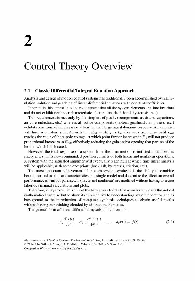
or a pair of complex conjugates. Taking an initial guess at the real root and using successivesynthetic divisions will eventually result in a solvable quadratic, producing the three roots.


unknown10 x pow

x 3

2

+++

constraint

-1.

-2.

constraint

+++

2

3y

powy-10 unknown

Solve: x^2+3x+2=0

(y=x)

Answer: x = -1

Answer: x = -2

1st Estimate

2nd Estimate

Figure 2.1 Quadratic solution by simulation

Similar techniques allow manual solving of higher order equations, but this approach isno longer necessary since computer programs and simulations (MATLAB R©, VisSim) areavailable that provide rapid, accurate solutions.

Figures 2.1–2.4 show VisSim solution diagrams of sample quadratic and cubic equations.Note in Equations 2.1 and 2.2 the equations are “solved” by constructing them, using standardsimulation blocks. The routine then starts with the initial estimates and continually calculatesthe equation until an answer of “0” is reached within a defined error restraint. Figures 2.3 and2.4 use a more powerful polynomial solver.

2.2 LaPlace Transform-the S Domain

Since the solving of the differential/integral equations describing a motion system can be quitelaborious, except for first and second order systems, the use of the LaPlace transform allowsone to solve the equations by converting them from the time domain to the frequency domain.

The LaPlace transform, for engineering purposes, is usually stated as:

F(S) =∫ ∞

0e−St f (t)dt (2.14)

where S is the complex variable, δ + jω; ω = 2π f ; f is in Hz.Tables of direct and inverse transforms for use in LaPlace operations are readily available

in control systems text books and handbooks.The result is that calculus calculations become algebraic calculations.The algebraic solution can be divided into a sum of common terms by partial fraction

expansion and each term can then be converted back to the time domain to display theoperation of the system in real time.


unknown-3 x pow

x 21

20

+--

constraint

-4.

5.

constraint

+--

20

21y

powy10 unknown

Solve: x^3 -21x -20=0

(z=y=x) Answer: x = -4

Answer: x = 5

unknown-2 z pow

z 21

20

+--

constraint

-1.

Answer: x = -1

1st Estimate

2nd Estimate

3rd Estimate

Figure 2.2 Cubic solution by simulation

-1.-1.

1.-1.

Coef sReal

Imag

PolyRoots

[1 2 2 ]

Solve; X^2 +2X +2 = 0

Figure 2.3 Quadratic solution by Poly Roots solver

-1.-1.-3.

1.-1.0

Coef sReal

Imag

PolyRoots

[1 5 8 6 ]

Solve; X^3 +5X^2 +8X +6 = 0

Figure 2.4 Cubic solution by Poly roots solver


Returning to the mechanical system in Section 2.1, the LaPlace solution would proceed asfollows:

Jdθ ′

dt+ Bθ ′ = T (2.15)

JSθ ′(S) + Bθ ′(S) = T

S(2.16)

θ ′(S) [JS + B] = T

S(2.17)

θ ′(S) = T

S (JS + B)= T/J

S (S + B/J )= A1

S+ A2

(S + B/J )(2.18)

A1 = T/J

B/J= T

BA2 = T/J

−B/J= − T

B(2.19)

θ ′(S) = T/B

S− T/B

(S + B/J )(2.20)

θ ′(t) = T

B

(1 − e− B

J t)

(2.21)

Note how the partial fraction expansion leads directly to the “complementary” and “particular”solutions described previously when reviewing the classical approach.

Note also, this solution assumed zero initial conditions, in which the acceleration term dθ ′dt

transforms to Sθ ′(S). The exact transform, showing initial conditions is Sθ ′(S) − f (0), wheref(0) is the initial condition. This would lead to an exact solution [3] of:

θ ′(t) =[

f (0) − T

B

]e− B

J t + T

B(2.22)

which reduces to Equation 2.12 if f(0) = 0.In other words, if this system has an initial velocity at the time the torque step is applied,

the initial velocity value will exponentially decay at the same rate that the new and final valuedevelops.

Solving a differential equation using the LaPlace transform involves four basic steps:

1. Transform the individual terms of the differential equation, including initial conditions.2. Solve the transformed equation for the unknown.3. Form the partial fraction expansion.4. Form the total solution as the sum of the individual inverse transforms of the partial fraction

terms.


2.3 The Transfer Function

The transfer function of any component or assembly, H(S), is the ratio of the transform of itsoutput, F(S)out, to the transform of its input, F(S)in.

H (S) = F(S)out

F(S)in(2.23)

In the mechanical system being evaluated:

H (S) = 1

SJ + BF(S)in = T

S∴ F(S)out =

[1

SJ + B

] [T

S

](2.24)

A simple powerful tool provided by the concept of the transfer function, since it is a linear alge-braic function and superposition holds, is the ability to manipulate and simplify combinationsof transfer functions into a single unit, especially in the case of feedback loops [4].

ExamplesTwo transfer functions in series (Figure 2.5)

11

s+21

1

s+31

1

s2+5s+6

Figure 2.5 Series transfer functions combined

Two transfer functions in parallel (Figure 2.6)

11

s+2

11

s+3

12s+4

s2+5s+6

++

Figure 2.6 Parallel transfer functions combined

Transfer functions in parallel and series (Figure 2.7).

11

s+2

11

s+3

12s+4

s4+14s

3+71s

2+154s+120

++ 1

1

s+41

1

s+5

Figure 2.7 Series/parallel transfer functions combined


A second interesting aspect is to be able to manipulate transfer functions in a simulation toquickly observe the effect of component variations, both linear and nonlinear, on the operationof the system, without resorting to complex mathematics.

For example, Equation 2.7 was solved using the implicit solution:

∫dx

a − bx= 1

−bln (a − bx)

However, as mentioned in Section 2.1, conditions could exist which would require a solutionof: ∫

dx

a − bxn

At this point, instead of searching for a general implicit solution for this integral, and since aspecific system is being designed, it is more efficient to directly simulate the transfer functionin such a manner as to be able to display the velocity profile and to determine the effect the“n” factor will have on various parameters.

The transfer function can be simulated as shown in Figure 2.8 in which the viscous dampingterm has been isolated in order to show the effect of the “n” term.

11

Js+B

+- 1/J 1/S

B

T VelocityT

velocity=

Figure 2.8 Transfer function with B term isolated

Figure 2.9a shows the velocity response for a system with the following parameters:

J = 0.19 g cm s2 B = 0.95 g cm rad−1 s−1 T = 100 g cm n = 1

with the steady-state velocity becoming 105 rad s−1 (1000 rpm)Figures 2.9b, c and d show the results with n = 1.2, 1.4 and 1.6, respectively.The following table lists the torque (T) necessary to maintain the final velocity at 105 rad s−1

and the resultant time constant for each of the four conditions:

n T (g cm) Time constant (ms)

1 100 2001.2 254 801.4 645 301.6 1650 10

This example shows how the use of simulation, which allows manipulation of systemparameters and use of a “what if” approach provides rapid results in comparison to a strictlymathematical analysis.

electromechanical motion systems - design and...

Documents