electron density and collision frequency of microwave

Electron density and collision frequency of microwave-resonant-cavity- produced discharges

W. McCall, C. Brooks, and M. L. Brake Department of Nuclear Engineering, University of Michigan, Ann Arbor, Michigan 48109-2104

(Received 22 February 1993; accepted for publication 4 June 1993)

A review of perturbation diagnostics applied to microwave resonant cavity discharges is presented. The classical microwave perturbation technique examines the shift in the resonant frequency and cavity quality factor of the resonant cavity caused by low-electron density discharges. However, the modifications presented allow the analysis to be applied to discharges with electron densities beyond the limit predicted by perturbation theory. An “exact” perturbation analysis is presented which models the discharge as a separate dielectric, thereby removing the restrictions on electron density imposed by the classical technique. The ‘iexact” method also uses measurements of the shifts in the resonant conditions of the cavity. Third, an electromagnetic analysis is presented which uses a characteristic equation, based upon Maxwell’s laws, and predicts the discharge conductivity based upon measurements of a complex axial wave number. By allowing the axial wave number of the electromagnetic fields to be complex, the fields are experimentally and theoretically shown to be spatially attenuated. The diagnostics are applied to continuous-wave microwave (2.45 GHz) discharges produced in an Asmussen resonant cavity. Double Langmuir probes, placed directly in the discharge at the point where the radial electric field is zero, act as a comparison with the analytic diagnostics. Microwave powers ranging from 30 to 100 W produce helium and nitrogen discharges with pressures ranging from 0.5 to 6 Torr. Analysis of the data predicts electron temperatures from 5 to 20 eV, electron densities from 10” to 3 X lOI cmm3, and collision frequencies from lo9 to 10” s-‘*

1. INTRODUCTION

Microwave resonant cavity discharges and electron cy- clotron resonance (ECR) discharges have become increas- ingly useful in industrial processes. The low-pressure, low- ion energy characteristics of ECR discharges make them promising alternatives to radio-frequency-coupled devices in the field of plasma processing of materials. Due to the inherent use of microwaves in ECR discharges, ECR de- signs utilizing microwave resonant cavity discharges are being extensively studied for use in plasma processing and thin-film deposition. ’

Resonant cavity discharges have many additional applications other than materials processing, such as fluores- cent excimer lamp systems2J3 and as a possible laser medium.4 Due to the lack of electrodes, resonant cavities are very durable yet simple in design and operation. The availability of inexpensive microwave components at 2.45 GHz is also an attractive feature.

Prior to 1970, the electromagnetics of microwave resonant cavities perturbed by discharges was extensively studied.s-22 An article published in 1946 by Slate? extensively details research on microwave electronics completed during World War II at the Massachusetts Institute of Technology. The article details the effects that an arbitrary conductance places on a microwave resonant cavity. The techniques presented by Slater were then applied specifi- cally to plasma dischargesg8 These initial techniques were actually used with repetitively pulsed discharges, either formed by the electromagnetic fields within the cavity or produced externally. In a series of four articles by Brown

and co-workers,s-‘2 the Slater technique was extensively detailed, as well as its applications as an electron density and collision frequency diagnostic of externally produced discharges.

The Slater technique, commonly referred to as perturbation analysis, determines the shifts in the resonant conditions of the microwave cavity due to a complex conductivity present in the cavity. The real portion of the conductivity causes a shift in the cavity quality factor while the imaginary portion shifts the resonant frequency of the cavity. Discharge theory then relates the complex conductivity to the electron density and electron-neutral collision frequency.

Perturbation analysis in its original form does not ad- dress the implication the discharge places on the electromagnetic fields. When analyzing the lumped cavity- discharge circuit, the electric fields are assumed to be those of an empty cavity. In this way, the complex dielectric constant of the discharge is ignored and the discharge and resonant cavity circuit are treated by electronic circuit theory. While this simplification is justifiable for low-electron- density, low-pressure discharges, it becomes a major source of error for high-density discharges. These errors were an- alyzed in an article published in 1957 by Persson,13 in which the limits of perturbation analysis are studied and details of how to slightly extend these limits are presented. In a contemporaneous publication, Buchsbaum and Brown14 demonstrated experimentally which resonant cavity modes are appropriate for high-density discharges, and determined for S-band microwaves the upper limit of al- lowable electron density, namely 1012 cma3.

3724 J. Appl. Phys. 74 (6), 15 September 1993 0021-8979/93/74(6)/3724/12/$6.00 0 1993 American Institute of Physics 3724

One refinement of perturbation analysis is to include the spatial variations of the plasma discharge.‘s*‘6 This technique was actually presented as a method to determine the spatial profile of low-density discharges; however, this procedure also demonstrates a reduction of the errors inherent in perturbation analysis.

Developed after the perturbation analysis is the so- called “exact” theory, 17-20 a method that was actually applied to waveguide discharges as early as 1947.21,22 In this procedure, the plasma discharge is included in the resonant cavity as a separate dielectric. By matching the electromagnetic field boundary conditions along the surface of the discharge as well as at the cavity walls, a characteristic equation is obtained. Solutions of the characteristic equation provide the conductivity of the discharge as a function of the shift in the resonant frequency of the cavity. If the collision frequency is not zero, the electromagnetic fields become complex which greatly complicates the characteristic equation. The effect of electron collisions was ad- dressed by expanding the characteristic equation solutions in a Taylor series about the zero collision frequency solutions. However, the exact theory is applicable to high- density discharges since the characteristic equation models the electromagnetic fields in the presence of a discharge. This is a departure from Brown’s treatment of the discharge as a lumped circuit element.

The basic premise of the electromagnetic analysis presented here, similar to recently developed models,‘3-26 is to model the discharge as a lossy dielectric produced in a reduced density gas channel by absorbing microwave power delivered to a surrounding resonant cavity. This departs from the perturbation analysis and the exact theory since the discharge is formed by the resonant cavity fields, rather than simply placing a resonant cavity around an existing discharge. Maxwell’s equations are solved in all regions of the cavity by assuming that the cavity is excited in a specific electromagnetic mode and that the forward and backward traveling electromagnetic waves have a complex axial wave number. This is unlike previous models17-20’23 which have assumed a real wave number but a complex microwave frequency. A complex axial wave number is required to account for the attenuation of microwaves as they propagate along the discharge, as well as the absorption of microwave power by the discharge. De- tails of the electromagnetic analysis are given in the following section.

Nonintrusive diagnostics, in addition to the modeling of the electromagnetic fields in the cavity, have been applied to resonant cavity discharges to measure various characteristics. These include laser-induced fluorescence diagnosticsZ7 and emission spectroscopy studies,‘* as well as the application of a Langmuir probe directly into the discharge within the resonant cavity.29 This article also presents a review of classical microwave cavity diagnostic techniques and compares these with more extensive ver- sions. The results of double Langmuir probes applied to a resonant cavity discharge are compared with cavity perturbation analyses and the electromagnetic analysis of the fields in the cavity.

3725 J. Appl. Phys., Vol. 74, No. 6, 15 September 1993

region X region Y

I region 3 I

I microwave I

coupling I

Z=O z=L,“t z=L

FIG. 1. The various regions utilized by the electromagnetic analysis. The basis of the analysis is that the electromagnetic fields are spatially attenuated as they move away from the microwave coupling antenna.

II. ELECTROMAGNETIC ANALYSIS

The purpose of this analysis is to model a discharge that is created by absorption of energy contained in electromagnetic fields in a resonant microwave cavity. As the electromagnetic fields travel along the dissipative discharge, they become spatially attenuated. This type of attenuation requires a complex axial wave number while the microwave frequency is kept real and constant. The resonant cavity used in this experiment is tuned by shifting the length of the cavity, rather than by varying the microwave frequency. The mode configuration studied is a transverse magnetic (TM0i2) mode, although this analysis may be modified for use in other cavities and modes.

A diagram of the geometry used in the analysis is shown in Fig. 1. In the analysis, outlined in Fig. 2, the resonant cavity is divided into three regions: (i) the par- tially ionized discharge produced in a gas channel contained by a quartz tube; (ii) the containment vessel (quartz); and (iii) the free space extending from the containment vessel to the cavity walls. It is assumed that the discharge fills the vacuum vessel and that the regions are isotropic and continuous along the axis of the cavity. Elec- tromagnetic fields based upon a TM,,, mode are derived for the three regions using Maxwell’s equations. The presence of the discharge affects both the wave number of the electromagnetic fields and the permittivity of the discharge, which become complex in value.

Boundary conditions are used to relate the electromagnetic fields at the interfaces of the different regions. These relations are used to produce a characteristic equation, the roots of which provide the electrical permittivity of the discharge. By knowing the wave number of the discharge, which is found using the length of the cavity and the attenuation of the electromagnetic fields, these roots may be

McCall, Brooks, and Brake 3725

measure: power absorbed by plasma electric fields at cavity wall -1

[ti] e2 1

eme(v+jw)

i / power input=$%e fg(oEjdV.

i gives magnitude of electric fields in cavitv

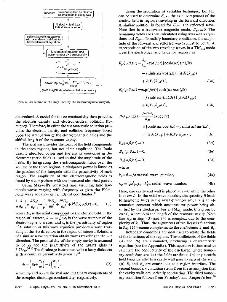
FIG. 7. An outline of the steps used by the electromagnetic analysis.

determined. A model for the ac conductivity then provides the electron density and electron-neutral collision frequency. Therefore, in effect the characteristic equation provides the eIectron density and collision frequency based upon the attenuation of the electromagnetic fields and the shifted length of the resonant cavity.

The analysis provides the form of the field components in the three regions, but not their amplitude. The Joule heating absorbed power and the energy contained in the electromagnetic fields is used to find the amplitude of the fields. By integrating the electromagnetic fields over the volume of the three regions, a dissipated power is found as the product of the integrals with the permittivity of each region. The amplitude of the electromagnetic fields is found by a comparison with the measured absorbed power.

Using Maxwell’s equations and assuming time harmonic waves varying with frequency w gives the Helm- holtz wave equation in cylindrical coordinates,30

+~E,(p,e,z) ~0, (1)

where E, is the axial component of the electric field in the region of interest, k = o 6 is the wave number of the electromagnetic waves, and ei is the permittivity of region i. ‘A solution of this wave equation provides a wave traveling in the +z direction in the region of interest. Solutions of a similar wave equation obtain waves traveling in the -z direction. The permittivity of the empty cavity is assumed to be e. and the permittivity of the quartz glass is 3.78~~. 26730 The discharge is assumed to be a lossy dielectric with a complex permittivity given by3i

(2)

where CT, and a, are the real and imaginary components of the complex discharge conductivity, respectively.


Using the separation of variables technique, Eq. (1) can be used to determine Ezi+ , the axial component of the electric field in region i traveling in the forward direction. A similar solution is found for Ed-, the reflected wave. Note that in a transverse magnetic mode, B,*tO. The remaining fields are then calculated using Maxwell’s equations and E,ia . To satisfy boundary conditions, the amplitude of the forward and reflected waves must be equal. A superposition of the two traveling waves in a TMei2 mode gives the electromagnetic fields for region i as

Epi(p,e,z,t) =k bk exp( jot) [cosh(crz)sin(fiz) pi

-j sinh(4cosW) I [A?1 (kpip)

+BiYlCkpip)l,

E,(p,0,Z,t) =exp( jut) [cosh(az)~~~(fl~)

-j sinh(oz)sin(flz)] [A&k,,p)

+BiYo(kpip)l,

(34

(3b)

&(p,&sf) = jWo6 - exp( jot) k

pi

X[A~~J,(kpip>+BiY*(kpip>l,

E&,&w) -0,

Bpi(p,e,zJ) ~0,

Bzi(p,O,z,d =O,

where

(3c)

(3d)

(3e)

(W

k==fi- jaGaxial wave number, (44

kpi= ,/mz=radial wave number. (4bb)

Here, one cavity end wall is placed at z=O while the other is at z= L. In the axial wave number, the quantity fl leads to harmonic fields in the axial direction while (31 is an attenuation constant which accounts for power being absorbed by the discharge. For a TM,*, mode, fi is given by h-/L, where L is the length of the resonant cavity. Note that kpi in Eqs. (3) and (4) is complex, due to the com- plexity of kz. Thus, the arguments of the Bessel’s functions in Eq. (3) become complex as do the coefficients Ai and Bi.

Boundary conditions are now used to relate the fields at the interfaces of the regions. The coefficients of the fields (Ai and Bi) are eliminated, producing a characteristic equation (see the Appendix). This equation is then used to calculate the conductivity of the discharge. These boundary conditions are: (a) the fields are finite; (b) any electric field lying parallel to a cavity wall goes to zero at the wall; (c) i& and Be are continuous at a region interface. The second boundary condition stems from the assumption that the cavity walls are perfectly conducting. The third boundary condition follows from Faraday’s and Ampere’s law.30

fvIcColi, Brooks, and Brake 3726

z-‘/z

cavity length

FIG. 3. Samples of the radial electric field (e), as well as the standing wave predicted by the electromagnetic analysis (solid line). The attenuation of the standing wave is a result power being absorbed by the discharge. The null position in the middle of the cavity is utilized to insert double Langmuir probe wires into the discharge.

Due to the second boundary condition, the radial electric field should be equal to zero at both ends of the cavity, i.e., at z=O and at z= L. Two waves will add to zero only if the waves have equal magnitude, an assumption already made in Eq. (3). This also requires that the quantity fi must be an integer multiple of s-/L while the quantity a must be zero, i.e., the axial wave number must be completely real.

Past studies have remained true to this condition by ignoring any spatial attenuation of the electromagnetic fields. This requires that the microwave frequency be complex, while maintaining a real axial wave number. A complex frequency leads to temporally damped fields, while a complex axial wave number provides spatially attenuated fields. Spatial attenuation implies a reference point from which the fields are attenuated, even though it has been assumed that the cavity is symmetric. Therefore, in a perfectly symmetric cavity there can be no spatial attenuation.

In practice, however, there is spatial attenuation of the electromagnetic fields. The reason for this is simple: in practice the cavity is not perfectly symmetric. The reference point for this asymmetry is the port or antenna from which the microwaves are launched into the cavity, as illustrated in Fig. 1. To account for this asymmetry, the cavity is broken into two regions in the axial direction: (i) region X which extends from one cavity wall to the microwave coupling antenna (0 <z < L,,J, and (ii) region Y which extends from the antenna to the other cavity wall ( L,, <z < L). The boundary conditions are met by assuming that the radial electric field is zero at z=O in region X and at z= L in region Y, while continuous at the interface at z= L,,, . Solutions based upon this assumption still satisfy Maxwell’s equations as well as Eq. ( 1) and are presented in the Appendix. A spatially attenuated standing wave is shown in Fig. 3 as well as samples of the radial electric field taken at the wall of the cavity using an electric-field probe, which verifies that the attenuation is a spatial phenomenon. The electric-field probe samples the


square of the magnitude of the radial electric field at various positions along the length of the cavity.

The characteristic equation is a complex equation, the roots of which provide the conductivity of the discharge as a function of the axial wave number, calculable from experimental data. Discharge theory provides a theoretical model of the conductivity for comparison with the solutions of the characteristic equation. If the electron-neutral collisions are elastic and the distribution function is uni- form, the conductivity becomes3’

4~ e2

s

a ~~(afo/a~) "=i=G? 0 v(v) + jw dv' (5)

where f. is the first term of an expansion of the electron distribution function and Y(V) is the electron collision frequency. Typically, Y(V) for different gases is a function of the electron velocity v, and Eq. (5) becomes a function of the electron distribution fo. To overcome this dependence, an effective collision frequency may be defined as31V3’

(6)

Using this effective collision frequency, the conductivity becomes

a=oR+ jo,, (74

veff

ng2 w aI= _-

m, [(~~d~-t-~~l ’

U’b)

(7c)

Once the conductivity is found using the characteristic equation, it can be substituted into Eq. (7) and the electron density and effective electron collision frequency may be determined.

The time-averaged power dissipated is found by

+ 7 Jr,,. i ~Eilgi12dv*

The first term represents a Joule heating term of the discharge while the second term represents the energy stored in the electromagnetic fields in the three regions and dissipated in the cavity walls. The electric fields are known to within a constant, their amplitudes Ai and Bi. By use of the boundary conditions, these coefficients may be related to A,. The electric fields, conductivity, and permittivities may then be integrated over the cavity leaving a value multi- plied by the square of the amplitude of the electromagnetic fields ) Al 1 2, the product of which provides an absorbed power. This power is now compared with the measured input power, and the coefficient 1 Al 1 is adjusted until the

McCall, Brooks, and Brake 3727

two powers match. Once this is completed, the magnitude of all of the electromagnetic fields throughout the microwave cavity may be calculated.

III. CAVITY PERTURBATION

A. Classical perturbation technique

Microwave cavity perturbation diagnostics depends upon the conductivity of the discharge in question to de- tune the resonant cavity. By measuring the amount of de- tuning, both the electron density and the electron collision frequency may be determined. The shift in the resonant conditions is given by5

- -

(9)

where 7 represents the current density and ,@ represents the electric fields present within the cavity. All of the integrals are over volume V. The subscript 0 refers to conditions in the cavity without a discharge present. The shift in the resonant frequency of the cavity caused by the discharge is Aw and Q is the cavity quality factor.

The electric fields present in an unloaded cavity are given by3’

(lOa>

&dp,B,z) =a

(lob)

(1Oc)

Typically, Ohm’s law is used to represent the current density [i.e., r=& where the conductivity D is given by Eq. (7)] and the real and imaginary components of Eq. (9) provide calculations of the electron density and effective collision frequency.

Generally, perturbation techniques are not applicable to high-density (n, > 5 x lo9 cmm3) dischargesI For low- density discharges, the plasma frequency is much less than the microwave frequency and the effect of the discharge on the electric fields is small. In this case, E-E0 is replaced by 1 go ( 2 that is, the electric fields in the presence of the discharge are approximately the same as those of an unloaded cavity. As the plasma frequency approaches the microwave frequency, this is less likely the case and the errors involved become intolerable. However, it has been shown’3*‘4 that in certain cases densities up to lOI cmm3 may be accurately measured with this technique. In particular, if the electric fields lie perpendicular to any electron density gradients the technique can be used at high densities. The phrase “classical perturbation” is used here to designate the use of z*zo= \,!?o;0,2 in Eq. (9).

Measuring the cavity Q in the presence of a discharge is a difficult and inaccurate process. To do this requires the superposition of a variable frequency microwave signal with the fixed frequency cw signal and sweeping the frequency while monitoring any reflected signal. This may be accomplished using various experimental configurations. However, the reflected cw signal usually overwhelms any reflections due to the variable frequency signal, resulting in a very poor signal-to-noise ratio. To overcome this the definition of the cavity Q, given below, is utilized:30

Q=co energy stored

energy dissipated’ (11)

The energy stored is simply proportional to the square of the electric fields,30 measurable using a simple electric-field probe. The energy dissipated can also be measured. There- fore, the cavity Q in the presence of a discharge is approximately26

(12)

where the subscript 0 refers to conditions in the cavity without a discharge present, P, is the dissipated energy, and 1 Epwl ’ represents the electric-field probe measurements, typically sampled at the wall of the cavity. To measure the shifted resonant frequency, the discharge is ignited and the cavity is tuned by minimizing the reflected microwave power. The discharge is then turned off and the resonant frequency is measured without readjusting the cavity length. In this way both ho and Q can be measured and the electron density and collision frequency can be calculated.

The classical perturbation integrals in Eq. (9) can be calculated using the electric fields given in Eq. (10) by assuming that E* Eo= ] El 2. Since the electron density is included in the integrals, a functional form for the electron density may be included to permit integration along with the electric fields.*53’6 This is done to minimize the error of the classical perturbation technique. Since the time- averaged power dissipated is proportional to the square of the electric fields, and the electron density in general follows the dissipated power, it is assumed that the electron density follows the electric fields squared [see Eq. (lo)]. Note, however, that the radial component of the electric field is close to zero at the center of the cavity where the discharge is present [due to J1 ( p = 0) = 01, and thus may be ignored. Therefore, the electron density can be assumed to follow the square of the axial component of the electric field, or

This is further supported by fiber-optic probe data, used to measure the optical emission as a function of axial position. In general, the optical emission follows co? (2m/ L ) . Since the electron density follows the electric field, the fields are

3728 J. Appl. Phys., Vol. 74, No. 6, 15 September 1993 McCall, Brooks, and Brake 3728

s ‘G 2 E E .g

1

b

cavity length

FIG. 4. Samples of the light emitted by a discharge as a function of position along the cavity axis (8). The discharge is bounded axially by the positions L,,,,, and L,,,,, and in general follows cos’(27rz/l) (solid line).

not perpendicular to any density gradients. However, as will be shown, application of perturbation techniques to densities above 10’ crnu3 is justified.

Since the discharge is not confined in the axial direction, the plasma does not always fill the entire length of the resonant cavity. The bounds of the discharge therefore run radially from p=O to the inner wall of the vacuum vessel, and axially from some position z= Lstart to z= Lstop. The quantities L,,, and Lstop are the experimentally measured physical bounds of the discharge. These are demonstrated in Fig. 4, which shows data of the light emission of a discharge. Using the functional form of the electron density given in Eq. ( 13), the integrals in Eq. (9) are calcti- lated for each particular experimental situation. Combined with the complex conductivity, the real and imaginary components are equated to the shifts in the resonant frequency and cavity Q.

It is interesting to note that as the length of the discharge changes, the integral of the electric fields over the plasma volume also changes. Therefore, the proportional- ity constant predicted by the classical technique (i.e., ho= kn,) decreases with plasma volume. By including this variation in plasma length, the classical perturbation technique may yield reasonably accurate results at higher electron densities ( > lo9 cme3).

B. Exact perturbation technique

As was shown in the previous subsection, it is possible to calculate solutions for the electromagnetic fields in the presence of a discharge. These solutions may then be used in Eq. (9)) removing the conditions restricting the electron density; however, it is difficult to solve Eq. (9) analytically, since it involves Bessel functions of complex arguments. A derivation presented in the Appendix shows that in the presence of a discharge, the perturbation equation becomes simply

c (8. B+po&@dV=O, (14) J cavity

which can be solved numerically. Note that the electromagnetic fields are dotted with themselves, not with their complex conjugates, so that the dot products are not necessarily positive definite quantities. In this way the integrals of the complex Bessel functions reduce to equations that are solved using a complex root finding routine. Here the microwave frequency is allowed to be complex and shift, with

m=tiR+ jwr, (Isa>

OR 1 ol=-A - . 0 2 Q (15b)

Fields similar to those shown in Eq. (3) may be used in Eq. (14) for an “exact” perturbation analysis. Unlike the classical perturbation technique, which uses a spatial electron density profile as in Eq. ( 13), the exact analysis assumes the discharge is isotropic and continuous throughout the discharge region. To analyze an electron density that varies with position, the arguments of the Bessel functions in Eq. (3) become functions of position which greatly complicates the exact analysis.

The exact theory first introduced by Brown17 is actually an electromagnetic analysis, similar to the one presented in the previous subsection, since it matches boundary conditions to obtain a characteristic equation. Equation (14) is a perturbation technique, since it deals with the integration of the electromagnetic Aelds over the volume of the cavity. Also, in Brown’s exact theory the effects of the collision frequency were ignored to ensure that the electromagnetic fields remain real. The presence of a collision frequency causes the discharge permittivity to become complex and complicates the analysis. Both the electromagnetic analysis and exact perturbation analysis presented here deal with the collision frequency directly, since no restrictions are placed on the collision frequency and the fields are not restricted to being completely real.

The electron density predicted by the classical and exact perturbation analysis is illustrated in Fig. 5. The solid line represents solutions predicted by the exact analysis. The dashed line is from the classical theory for a discharge that entirely fills the cavity, while the dashed line with circles is for a discharge that fills half the cavity, centered in the middle. Classical perturbation theory [Eq. (9)] predicts that the electron density varies linearly with the frequency shift, while the exact analysis [Eq. ( 14)] predicts a departure from this linearity above electron densities of 5 X 10” cmm3. This agrees with- the well known work of Brown and co-workers17*18 which predicts a departure around 1012 cme3 for a TM,,, mode. However, the electric fields of the TM,,, mode are completely perpendicular to any density gradients, as opposed to those of the TM,,, mode. Also note that the classical and exact perturbation method do not give precisely the same results below 5X 10” cm 3. This is because the exact technique presented here accounts for the effect of the dielectric constant of the quartz tube, while the classical treatment does not.


I

10 " 10'2

electron density (cmm3)

FIG. 5. The shift in the microwave frequency for various electron densities for a TM&, mode. The resonant microwave frequency is 2.45 GHz. The solid l ine corresponds to solutions from the “exact” technique. The dashed line is from the classical perturbation technique for a p lasma that fills the length of the cavity, while the dashed line with circles corresponds to a discharge tilling half the cavity. The exact technique accounts for the presence of the quartz tube, while the classical technique does not.

IV. EXPERIMENT A. Experimental technique

In this experiment, helium and nitrogen discharges were contained in a quartz tube (25 mm i.d., 28 mm o.d.) placed along the axis of an Asmussen33Y34 resonant cavity operating in a transverse magnetic (TM,,,) mode. The cavity walls are constructed of brass, and therefore highly conductive. The inner radius of the cavity is 8.9 cm, but the length of the cavity may be varied from 6 to 16 cm by use of a sliding short. Variations in the cavity length are necessary because the presence of the discharge shifts the resonant conditions of the cavity. A microwave coupling antenna acts as a variable impedance transformer between the waveguide carrying the microwaves and the resonant cavity. The microwave coupling antenna is designed such that the depth at which the antenna is inserted into the cavity is variable. Both the sliding short and the coupling antenna are varied until the reflected power is minimized, typically to values less than 2% of the power supplied to the cavity. A schematic of the microwave cavity is shown in Fig. 6. Welded to one side of the cavity is a wire mesh

*i&3 vievl end Yiew

FIG. 6. A schematic of the Asmussen resonant microwave cavity used in the experiment. Variations in the cavity length are necessary to account for the perturbation caused by the discharge.

window, permitting viewing of the discharge and optical emission spectroscopy diagnostics.

Electric-field measurements are made by use of a simple electric-field probe. The electric-field probe consists of a short length of microcoaxial wire connected to a microwave power meter. The probe is inserted into small holes which run along the length of the cavity wall. It is arranged such that the inner conductor of the probe extends a few millimeters into the interior of the cavity. In this way, the probe measures a value proportional to the square of the magnitude of the radial electric field sampled at the wall of the cavity, or 1 EPw / 2.

The microwave circuit consists of a power source, a terminated three-port circulator, a bidirectional coupler and power meters, and the microwave cavity itself. Coaxial components are used throughout, with coaxial wave guides used to interconnect the components. The power source is a Micro-Now continuous-wave magnetron oscillator with a fixed frequency of 2.45 GHz and adjustable power from 0 to 500 w.

V. DOUBLE LANGMUIR PROBE

The electromagnetic fields in a resonant cavity are easily disturbed. If metallic probes are inserted into a cavity, their placement must ensure that the electric fields are not distorted. The electromagnetic fields of an unloaded cavity operating in a TM,,, mode were shown previously in Eq. ( 10). Due to the sin( 271z/L) dependence, the radial electric field at the plane z= L/2 is completely zero and the electric field lies only in the axial direction. It has been demonstrated29 that if the discharge does not perturb the general shapes of the fields, then it is possible to insert thin tungsten wires into these null positions to act as Langmuir probes. In this way the electric field lies only along the diameter of the wire, and the amount of microwave power absorbed by the wires is negligible. For other positions or orientations, the components of the electric field would lie parallel to the wire and the wire would act as an antenna, coupling the microwaves out of the cavity.

The cavity quality factor, or cavity Q, is a measure of how well a cavity stores the energy that is introduced to it. At the resonant frequency of a tuned cavity all of the in- cident power is absorbed by the cavity. Experimentally the resonant circuit Q is determined by9P30

(16)

where w. is the resonant frequency of the cavity and hw is the width of a swept frequency versus reflected power curve. When the cavity is tuned, the cavity Q is twice that of the resonant circuit Q.9 In this experiment the cavity Q without the Langmuir probe wires was approximately 6500 while with the probe wires it was roughly 5000. The theoretically maximum cavity Q of the resonant cavity is 15 5oo.30

One source of error in this experiment is the measurement of the surface area of the Langmuir probe wires. The


probes are afixed to the vacuum vessel using a ceramic vacuum seal, and tend to slip a small amount as the sealant dries. Once embedded, it is difficult to access the probes. The probe areas were less than 0.020 cm2 (typically a tungsten wire, with a radius of 0.041 cm and a length of 0.15 cm). A swept voltage circuit29 is used for acquiring the voltage-current characteristics.

B. Double-probe theory

Many articles and texts have been written on double- probe theory. 35-37 The two primary values derived from double-probe characteristics are the electron temperature and the ion density. An inherent assumption in double- probe theory is that the electrons of the discharge in question are described by a Maxwellian distribution. This may or may not be valid, but the assumption is the best available for the discharge described in this article. The theory also assumes that the probe radius is larger than the electron Debye length,35 a requirement that is met in this experiment (il9~0.003 cm, rP=0.04 cm).

The derivation of the electron temperature used in this experiment was first presented by Dote.37 The electron temperature is determined by the following:

T,( eV> = (0.244) ISI + IS2

dI/dVI v=o-0.82S ’ (17)

where dI/dV( V=O) is the slope at the inflection point, IS1 and Is2 are the saturation currents, and S is the slope of the curve in the saturation region. Typically some hysteresis is present, most likely due to probe contamination. The hysteresis does not diminish when the amplitude of the probe voltage is reduced. If the cause of the hysteresis were probe heating, then the opposite would be expected.

To determine the ion density, the Bohm criterion for ion saturation is used. The ion density is then given by3’

(O-61)1, M, ‘I2

==eA, T, ’ 1

( 1 (18)

where M, is the ion mass, I, is the saturation current, A, is the surface area of the probe, and T, is the electron temperature as found in Eq. ( 17). By the quasi-neutrality assumption, the electron density is estimated to be equal to the ion density.

VI. RESULTS

Langmuir probe data were obtained for discharges in both helium and nitrogen. Values required by Eqs. (17) and (18) are obtained from the voltage-current characteristics generated from the Langmuir probes. Electron temperature and ion densities are then calculated and shown in Figs. 7-10.

The electron temperature as a function of pressure obtained for helium and nitrogen discharges is shown in Fig. 7. The discharge power is set to a constant value of 65 W while the discharge pressure is varied. For low-pressure discharges, the electron temperature for. helium is larger than that of nitrogen discharges. The increase in electron temperature for low pressures is typical of rf discharges. At

5‘ ‘u E a F . d 10. E d 0 0 s 0 0 0 b 0 . . O 0 4 . a

01 I I 0 1 2 3 4 5

pressure (torr)

FIG. 7. The electron temperature as a function of pressure obtained for helium (0) and nitrogen (0) discharges.

low pressures, the electron temperature must increase to sustain a discharge since a decrease in the neutral density lowers the ionization rate. The actual error involved with these measurements is estimated to be sizeable because

‘d=d 0

.

t

(4 pressure (torr)

1P . , , , , , .~

@g .

A

z A

I lO=. .

8

s $ "!? m . x 4

.

A

m

A

II

A

A

q

A Id'1 * * ' ' '

0 1 2 3 4 5 6

(b) pressure (torr)

FIG. 8. (a) The electron density as a function of pressure at a constant power of 65 W obtained for helium determined by the double Langmuir probe (A.), electromagnetic analysis (O), classical perturbation technique (m), and “exact” perturbation technique (A). (b) The electron density as a function of pressure at a constant power of 65 W obtained for nitrogen determined by the double Langmuir probe ( A ) , electromagnetic analysis (O), classical perturbation technique (H), and “exact” perturbation technique (A).


H 4 c 6 t EL 4 s ‘ii, s 8

ld”

22 .

0 A A ::

30 40 50 60 70 60 90

(a)

10’3

-.@ c x

5 s 10’2

-0

s b P Q)

(a) pressure (torr)

‘“‘r------ ’ ’ ’ 10" ;

IO'O :

109 :

t

.

A

A

f

A

. A

n n

.

A

#

A

x

10SL. ’ ’ ’ ’ ’ 1 0 1 2 3 4 5 6

04 pressure (torr)

FIG. 9. (a) The collision frequency as a function of pressure at a constant power of 65 W obtained for helium determined by the double Langmuir probe (A ), electromagnetic analysis (O), classical perturbation technique (II), and “exact” perturbation technique (A). The solid line shows values predicted by Brown (see Ref. 39). (b) The collision frequency as a function of pressure at a constant power of 65 W obtained for nitrogen determined by the double Langmuir probe (A), electromagnetic analysis (O), classical perturbation technique (H), and “exact” perturbation technique (A).

double probes sample only the tail of the electron energy distribution. A high-energy tail will therefore lead to an overestimation of the electron temperature.

The electron density as a function of pressure at a constant power of 65 W in helium and nitrogen is shown in Fig. 8. The error bar shown in the electron density obtained from the Langmuir probe is an estimation of the error in the measurements due to the probable inaccuracy of the electron temperature. Obviously, there are other error components to consider.

Cavity perturbation and the electromagnetic analysis provide measurements of the electron density and collision frequency. To calculate collision frequencies from the Langmuir probe data, Eq. (6) is used. Assuming the electrons are described by a Maxwellian distribution and using the electron temperature obtained with the tloating probe, an effective collision frequency may be calculated by integrating Eq. (6) over the cross section for the gas in question. Due to the nature of the cross section for helium, the collision frequency for helium is predicted3’ to be proportional to the reduced pressure of the discharge.

power (watts)

. i A Af .A*

. q

f

q q

A A A

^^ ._ -. Y” 4” 50 60 70 60 90

Ib) power (watts)

FIG. 10. (a) The electron density as a function of power at a constant pressure of 10 Torr obtained for helium determined by the double Lang- muir probe (A), electromagnetic analysis (0). classical perturbation technique (m), and “exact” perturbation technique (A). (b) The electron density as a function of power at a constant pressure of 2 Torr obtained for nitrogen determined by the double Langmuir probe (A), electromagnetic analysis (O), classical perturbation technique (S), and “exact” perturbation technique (A).

The collision frequency as a function of pressure in helium and nitrogen is shown in Fig. 9. Values calculated using the Langmuir probe data are compared with those obtained by the electromagnetic analysis and cavity perturbation techniques. The solid line in Fig. 9(a) shows the collision frequency for helium as predicted by Brown.3g Generally the collision frequency increases with pressure. This is due to the fact that as the pressure increases, Y(U) in Eq. (6) increases with the neutral density since

Y(U) =Nva(u) cf , (19) s

where a(v) is the momentum transfer cross section, N is the neutral density, P is the discharge pressure, and T, is the neutral gas temperature. The collision frequencies obtained by the three diagnostics agree with this trend, although the values obtained with the electromagnetic analysis are disappointing. The assumption in the electromagnetic analysis of an isotropic discharge filling the length of the cavity may result in a large error.

The electron density as a function of power at a constant pressure is shown in Fig. 10. Data are shown for the


helium discharges at a fixed discharge pressure of 10 Torr, the discharge conductance places on the lumped while data for the nitrogen discharges are obtained at 2 discharge-microwave-cavity circuit. By assuming the elec- Torr. One interesting result is that the electron density tromagnetic fields are not affected by the discharge, the does not generally increase with the discharge power as microwave cavity is treated by electronic circuit theory. may be expected. As noted in similar experiments,24 as the Theory predicts that this assumption limits the use of the discharge power increases the volume of the discharge also classical analysis to low-electron density discharges; how- increases, thereby maintaining a constant power density. It ever, as shown in this article, inclusion of the spatial vari- is important to realize that with this type of experiment the ations of the electron density allow the analysis to be ap- volume of the discharge varies under different conditions plied to higher densities while incuring errors less than because the discharge is not bound in the axial direction. those predicted.

The collision frequencies for helium and nitrogen discharges (not shown) did not vary with power due to the constant pressure. Since the power density is roughly constant, the neutral gas temperature in Eq. ( 19) also does not change.

The major experimental sources of error are measurements of the discharge power, the frequency shifts, and the discharge volume. More fundamental sources of error are the assumptions inherent to the techniques. To estimate the experimental contribution to the error, solutions of the analyses may be found after varying the experimental input by reasonable amounts. For instance, an error in measurement of the cavity length or attenuation constant of approximately 5% leads to a half-order-of-magnitude differ- ence in the resulting electron densities. However, comparison of the data obtained with the three techniques indicates that despite the assumptions and measurement errors, there is rough agreement between the diagnostics. The classical and “exact” perturbation analyses yield similar results, even though the electron densities involved are well above the accepted limit.

To remove the limitations on the electron density, the discharge is treated from an electromagnetic standpoint. By modeling the discharge as a lossy dielectric, the electromagnetic fields in the presence of a discharge are determined. Boundary conditions governing the fields are then used to produce a characteristic equation. Solutions of the characteristic equation yield the complex conductivity of the discharge as a function of the perturbed resonant quantities of the cavity. Discharge theory then relates the conductivity to the electron density and collision frequency of the discharge. The electromagnetic analysis presented accurately accounts for the spatial attenuation of the electromagnetic fields. In contrast, prior analyses assume that the fields are temporally attenuated.

The corrected electromagnetic fields used in the electromagnetic analysis may also be used in conjunction with perturbation theory. This also eliminates the limitations of the classical perturbation technique. An “exact” perturbation integral is derived which predicts the shift in the microwave frequency necessary to compensate for the presence of the discharge.

The electron temperature measured by the double Langmuir probes actually comes from a sampling of the high energy “tail” electrons of the discharge. The electron temperature subsequently affects calculations of the ion density from the double probe data. Because the electron temperatures reported here are much higher than those generally found in rf discharges, it is reasonable that the actual electron densities are higher than those calculated from the double probe data.

It should also be noted that while the Langmuir probe obtains the electron density at fixed positions, the electron density obtained by the electromagnetic analysis and exact perturbation analysis is an average over the volume of the discharge. The classical perturbation technique uses an assumed spatial variation of the electron density; however, the other analyses ignore the spatial variations of the conductivity [see Eq. (7)]. Other techniques are available which take this into account,40 but these complexities have not been implemented into the present diagnostic.

The use of floating double Langmuir probes provides reasonable data which are consistent in trend with similar types of discharges, such as rf discharges. Disruption of the electromagnetic fields caused by the metallic probe wires is minimal, as shown by measurements of the cavity quality factor with the probe wires present. With the use of a simple sweeping circuit, the double Langmuir probes provide quick estimates of the electron density, electron temperature, and collision frequency of the resonant cavity discharge. These measurements are then easily compared with results from other diagnostics.

ACKNOWLEDGMENTS

The authors wish to thank Y. Y. Lau for his assistance regarding electromagnetic theory. This research is supported by DOE Grant No. DE-SG07-89ER12891.

VII. CONCLUSION

Diagnostic techniques are studied and applied to an Asmussen resonant microwave cavity to measure the electron density and collision frequency of resonant cavity discharges. Data are obtained through a range of operating pressures and powers in nitrogen and helium discharges.

The classical perturbation technique first introduced by Slater is studied. The classical analysis studies the effect

APPENDIX

Fundamental equation

The resonant cavity is broken into three radial regions: (i) the discharge; (ii) the quartz containment vessel; and (iii) the free space extending to the cavity walls. Boundary conditions applied to the electromagnetic fields at the interfaces of the regions may be displayed in matrix form, given by


Jdkpla) -Jdkp2a) - Ydkp2a) 0 0 Jo&,,@ Yo ( k,,b ) ~ Jo&& 0 0 0 Jo&,d

FJl(kpla) -5 Jl(k,,a) -?- Y,(k,,a) 0 Pl P2 %2

0

1 - YoW,3b) Yo(kp3c)

0

0 $ Jdkp2b) P2

F Jl(kp2b) P2

-$ Jdk,&) P3

--$ Yl(kp3b) P3

Setting the determinant of the first matrix equal to zero leads to the characteristic equation, given by

kp2E3C1 C3Y1(kp2b) +c4J1(kp2b) kp3E2C2=cJo(kp2b) +c4JO(kpZb) ’

where

YI (k,,b) cl=Jl(kp3b)-Jo(kp3c) yockp3c) ,

c2=Jo(kp& -Jdk,,c) Yo(k,& y (k

0 P3 c)

(A21

(ASa)

(A3b)

~3 = JI (k,,a) Jo(k,,a) cl E2

Jo(kpla) k,,-J,(kP2a) kp2 t (A3c)

Jl (k,,a) e1 C4=Yl(kp2a) $--Yo(kp2a) J (k ) k. Wd)

P2 0 p1a pl

et is found using Eq. (2), Ed= 3.78.5, (dielectric of quartz), e3 = eo, and the J’s and Y’s are Bessel’s functions of the first and second kind. The quantities a, b, and c are the radii of the three coaxial regions. The characteristic equation provides the conductivity of the tirst region as a function of the cavity length and attenuation of the electromagnetic fields.

The shifted cavity length as a function of the electron density predicted by the characteristic equation is shown in Fig. 11. It is interesting to note that the characteristic equation correctly predicts a new resonant cavity length, shorter than that of an unloaded cavity, when the cavity is loaded with the quartz vacuum vessel. The dielectric permittivity of the quartz tube is higher than that of free space causing an downward shift in cavity length, while the permittivity of a discharge is lower than that of free space causing an upward shift in cavity length.

Solutions of the characteristic equation show that as the attenuation constant approaches zero, the real portion of the conductivity also approaches zero. Because the dissipated power is proportional to the real component of the conductivity, the spatial attenuation is a direct result of the presence of the lossy material and results in power being absorbed by the lossy material.

Al A2

B2

A3

B3

0 0

= 0 . 0 0

(-4.1)

Electromagnetic fields

By introducing the axial regions to the fields shown in Eq. (3)) the electromagnetic waves in region X (0 <z< L.& remain the same as Eq. (3), while in region Y ( Lant <z < L) they are given by

EJ p,O,Z,t) = ---‘2 exp(jwt)sinh[ jk,(z-- L) ] P’

SinhI jk,(-Ld 1 ‘sinh[ jk,(L,,,- L)] [A21 (kpip)

+ BiYl (kpip )I 9 &(p,B,z,t) =exp(jwt)cosh[ jkZ(z-L)]

(AW

sinh( jk,L,,) ‘sinh[ jkz( Lant-- L)] [AJoJ,(k,id

+ BiYo(kpip> 13 (A4b)

Bdp,e,z,t) = kpi ‘Z5exp(jot)cosh[ jk,(z- L)]

sinh( jkZL,,& Xsinh[ jk,(L,,,-L)] [AJI (kpip J

+ BJl (kpip )I 9 (-44~)

electron density (1 O’* cm3) 0 0.75 1.5 2.25

17 I -- k

0 IO 20 30

cJ-lp/wo)

FIG. 11. The shifted cavity length for various electron densities predicted by the electromagnetic analysis at two collision frequencies. The resonant cavity length is 14.4 cm.


&(pA%sd =o, (Add) Bpi(p,eGGt) -0, (A4e)

&,(p,b,t) =a Wf) Shown in Fig. 3 is the standing wave predicted by these fields, as well as a set of electric-field probe data showing the attenuation present.

Cavity perturbation

such as a quantity dotted with its conjugate. Inspection of Eq. (A6) shows that the square of the magnetic field is negative, while the square of the~electric field is positive.

While Eq. (A8) may not look like a typical perturbation equation, the equation must hold at any frequency. The shift in the resonant frequency is a result of the presence of the discharge and the quartz vacuum vessel. In other words, for a given complex conductivity, the microwave frequency becomes complex and shifts such that Eq. (A8) still holds.

Assuming time harmonic electromagnetic waves, Max- well’s equations may be written as

VXE= -jai?, (ASa)

7X B=po(a+ jco,w)E. (A5b)

Assume that the presence of the discharge results in a microwave frequency shift and a complex frequency. The electromagnetic fields are then simply

~pi(~,B,z,t)=~exp(iOf)sin(kq) Pi

X[A~~Jkpif)+BiYl(k,ip)l, (AW ,?&(p$,z,t)=exp(jwt)cos(kg)

x MJoJo(k,ip) + W’o(k,id I, (A6b)

*pOei Bei(p,6JJ) =j 7 expUot)cos(ks)

pi

X [A~l(kpip)+BiY,(kpip)l, MC)

where k, and kpi are the same as in Eq. (4), except that now a is zero while the frequency o is complex.

Maxwell’s equations must hold whether or not there is a discharge present. If we take the dot product of the electric field with Eq. (A5b) and integrate over the volume of region i, we obtain

I ,!?* (vxB)dV=

IYgiOll s region i jruow~ l g d V. (A71

The first integral may be broken into two components, V l ( Bx E) + B. (V X E) . The second component is replaced using Eq. (A5a). The first component is solved using the divergence theorem, and becomes a surface integral over the surface of region i. However, at the interface of two regions, this integral will cancel, since the normal vector is in opposite directions while the fields are continuous at the interface. Therefore, if we sum Eq. (A7) over the three regions, the only surface integral left will be the one over the surface of the cavity walls. However, this surface integral is approximately zero due to the high conductivity of the cavity walls. What is left is then

r (B* B+po&@dV=O. (A81 J cavity

Here the dot product represents the square of complex quantities and is not necessarily a positive definite quantity,

‘J. Asmussen, J. Vat. Sci. Technol. A 7, 883 (1989). *T. Hatakeyama, F. Kannari, and M. Gbara, Appl. Phys. Lett. 59, 387

(1991). 3H. Kumagai and K. Toyoda, Appl. Phys. Lett. 59, 2811 (1991). 4W. McCall, M. Passow, and M. L. Brake, Rev. Sci. Instrum. 63, 1792

(1992). ‘J. C. Slater, Rev. Modern Phys. 18, 441 (1946). ?S. C. Brown et al, Technical Report No. 66, Research Laboratory of

Electronics, M.I.T., 1948. ‘D. J. Rose, D. E. Kerr, M. A. Biondi, E. Everhart, and S. C. Brown,

Technical Report No. 140, Research Laboratory of Electronics, M.I.T., 1949.

‘M. A. Biondi, Rev. Sci. Instrum. 22, 500 ( 1951). 9S. C. Brown and D. J. Rose, J. Appl. Phys. 23, 711 (1952).

“D. J. Rose and S. C. Brown, J. Appl. Phys. 23, 718 (1952). “D. J. Rose and S. C. Brown, J. Appl. Phys. 23, 1028 (1952). “L. Gould and S. C. Brown, J. Appl. Phys. 24, 1053 (1953). “K. B. Persson, Phys. Rev. 106, 191 (1957). 14S. J. Buchsbaum and S. C. Brown, Phys. Rev. 106, 196 (1957). “M. A. W. Vlachos and H. C. S. Hsuan, J. Appl. Phys. 39, 5009 ( 1968). t6C. J. Burkley and M. C. Sexton, J. Appl. Phys. 39, 5013 (1968). “S. C. Brown, in Proceedings of the 2nd U. N. International Conference

on Peaceful Uses of Atomic Energy, 1958, Vol. 32, p. 394. “S. .I. Buchsbaum, L. Mower, and S. C. Brown, Phys. Fluids 3. 806

(1960). 19B. Agdur and B. Enander, J. Appl. Phys. 33, 575 (1962). “J L Shohet and C. Moskowitz, I. Anal. Phys. 36, 1756 (1965). . . .___,. 2’ D. E. Kerr, S. C. Brown, and Kern, Whys. Rev. 71, 480 (1949). uP. Rosen, J. Appl. Phys. 20, 868 (1949). 23E. B. Manring; Ph.D. thesis, Michigan State University, 1992. 24W. McCall, M.S. thesis, University of Michigan, 1990. “M. L. Passow, M. L. Brake, P. Lopez, W. McCall, and T. Repetti,

IEEE Trans. Plasma Sci. PS-19, 219 (1991). 26J. Rogers, Ph.D. thesis, Michigan State University, 1982. “G King, F. C. Sze, P. Mak, T. A. Grotjohn, and J. Asmussen, J. Vat.

Sci. Technol. A 10, 1265 ( 1992). *sJ. Hopwood and J. Asmussen, Appl. Phys. Lett. 58, 2473 (1991). *‘W. McCall, C. Brooks, and M. L. Brake, J. Vat. Sci. Technol. A 11,

1152 (1993). ‘OR F Harrington, Time-Harmonic Electromagnetic Fields (McGraw- . .

Hill, New York, 1961). 3’B. E. Cherrington, Gaseous Electronics and Gas Lasers (Pergamon,

New York, 1979). ‘*R. F. Whitmer and G. F. Herrmann, Phys. Fluids 9, 768 ( 1966). 33 J. Asmussen, R. Mallavarpu, J. Hamann, and H. Park, Proc. IEEE 62,

109 (1974). 34R. Mallavarpu, J. Asmussen, and M. C. Hawley, IEEE Trans. Plasma

Sci. PS-6, 341 (1978). “J D Swift and M. J. R. Schwar, Electrical Probes for Plasma Diagnos- . .

tics (Iliffe, London, 1969). “E. 0. Johnson and L. Malter, Phys. Rev. 80, 58 (1950). “T. Dote, Jpn. J. Appl. Phys 7, 964 (1968). “N. Hershkowitz, in Plasma Diagnostics, edited by 0. Auciello and D. L.

Flamm (Academic, San Diego, 1989), Vol. 1. 39 S. C. Brown, Introduction to Electrical Discharges in Gases (Wiley, New

York, 1966). 4oS. Offermanns, J. Appl. Phys. 67, 115 (1990).


electron density and collision frequency of microwave

Documents