electronically - dms.psc.sc.gov
TRANSCRIPT
INTEGRATED RESOURCE PLANATTACHMENT IIIDUKE ENERGY PROGRESS2020 RESOURCE ADEQUACY STUDY
DUKE ENERGYPROGRESS 20
20
ELECTR
ONICALLY
FILED-2020
September1
4:43PM
-SCPSC
-Docket#
2019-225-E-Page
1of69
f5 DUKE4 ENERGY.
I&
4
aIN iii u
ii liII li
AI.II 4I ~ ~ ~
4 ~ ~ ~ -~
.;II ~ ~ - I
i +~ ~ Ig& ~ ~ sw
4. Ig Wl ~ 4y@&i',„Asi ~ .
~ 4 ~
p IJ ~ 3 ~
gal,~ ~~z
QaJLlii JEJg h.l IQIi LILYii AUlili A sIiil ~
ELECTR
ONICALLY
FILED-2020
September1
4:43PM
-SCPSC
-Docket#
2019-225-E-Page
2of69
YC' L
~ C is p igy g &y
1
+

Duke Energy Progress
2020 Resource Adequacy Study
9/1/2020
PREPARED FOR
Duke Energy PREPARED BY
Kevin Carden Nick Wintermantel Cole Benson Astrapé Consulting
ELECTR
ONICALLY
FILED-2020
September1
4:43PM
-SCPSC
-Docket#
2019-225-E-Page
3of69
A TRAPE CONS ULTINGinnovation in electric system planning

DEP 2020 Resource Adequacy Study
1
Contents Executive Summary ...................................................................................................................................... 3
I. List of Figures ......................................................................................................................................... 19
II. List of Tables .......................................................................................................................................... 20
III. Input Assumptions ................................................................................................................................ 21
A. Study Year ...................................................................................................................................... 21
B. Study Topology ............................................................................................................................... 21
C. Load Modeling ................................................................................................................................ 22
D. Economic Load Forecast Error ....................................................................................................... 28
E. Conventional Thermal Resources ................................................................................................... 29
F. Unit Outage Data ............................................................................................................................ 31
G. Solar and Battery Modeling ............................................................................................................ 33
H. Hydro Modeling .............................................................................................................................. 35
I. Demand Response Modeling .......................................................................................................... 37
J. Operating Reserve Requirements .................................................................................................... 38
K. External Assistance Modeling ........................................................................................................ 38
L. Cost of Unserved Energy ................................................................................................................ 40
M. System Capacity Carrying Costs ................................................................................................. 41
IV. Simulation Methodology ...................................................................................................................... 42
A. Case Probabilities ............................................................................................................................ 42
B. Reserve Margin Definition.............................................................................................................. 44
V. Physical Reliability Results.................................................................................................................... 45
VI. Base Case Economic Results ................................................................................................................ 49
VII. Sensitivities ......................................................................................................................................... 54
Outage Sensitivities ................................................................................................................................ 54
Load Forecast Error Sensitivities ............................................................................................................ 55
Solar Sensitivities.................................................................................................................................... 56
Demand Response (DR) Sensitivity ....................................................................................................... 57
No Coal Sensitivity ................................................................................................................................. 58
Climate Change Sensitivity ..................................................................................................................... 59
VIII. Economic Sensitivities ....................................................................................................................... 60
IX. DEC/DEP Combined Sensitivity .......................................................................................................... 61
X. Conclusions ............................................................................................................................................ 62
ELECTR
ONICALLY
FILED-2020
September1
4:43PM
-SCPSC
-Docket#
2019-225-E-Page
4of69
DEP 2020 Resource Adequacy Study
2
XI. Appendix A ........................................................................................................................................... 64
XII. Appendix B.......................................................................................................................................... 65
ELECTR
ONICALLY
FILED-2020
September1
4:43PM
-SCPSC
-Docket#
2019-225-E-Page
5of69
DEP 2020 Resource Adequacy Study
3
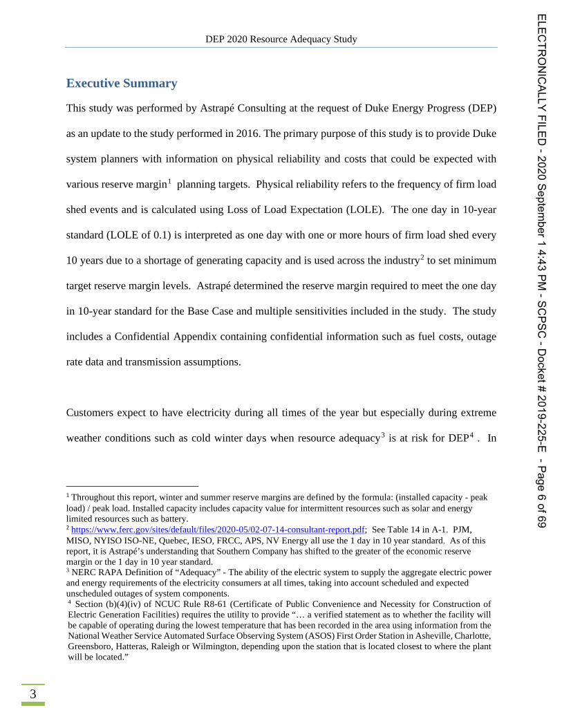
Executive Summary
This study was performed by Astrapé Consulting at the request of Duke Energy Progress (DEP)
as an update to the study performed in 2016. The primary purpose of this study is to provide Duke
system planners with information on physical reliability and costs that could be expected with
various reserve margin1 planning targets. Physical reliability refers to the frequency of firm load
shed events and is calculated using Loss of Load Expectation (LOLE). The one day in 10-year
standard (LOLE of 0.1) is interpreted as one day with one or more hours of firm load shed every
10 years due to a shortage of generating capacity and is used across the industry2 to set minimum
target reserve margin levels. Astrapé determined the reserve margin required to meet the one day
in 10-year standard for the Base Case and multiple sensitivities included in the study. The study
includes a Confidential Appendix containing confidential information such as fuel costs, outage
rate data and transmission assumptions.
Customers expect to have electricity during all times of the year but especially during extreme
weather conditions such as cold winter days when resource adequacy3 is at risk for DEP4 . In
1 Throughout this report, winter and summer reserve margins are defined by the formula: (installed capacity - peak load) / peak load. Installed capacity includes capacity value for intermittent resources such as solar and energy limited resources such as battery. 2 https://www.ferc.gov/sites/default/files/2020-05/02-07-14-consultant-report.pdf; See Table 14 in A-1. PJM, MISO, NYISO ISO-NE, Quebec, IESO, FRCC, APS, NV Energy all use the 1 day in 10 year standard. As of this report, it is Astrapé’s understanding that Southern Company has shifted to the greater of the economic reserve margin or the 1 day in 10 year standard. 3 NERC RAPA Definition of “Adequacy” - The ability of the electric system to supply the aggregate electric power and energy requirements of the electricity consumers at all times, taking into account scheduled and expected unscheduled outages of system components. 4 Section (b)(4)(iv) of NCUC Rule R8-61 (Certificate of Public Convenience and Necessity for Construction of Electric Generation Facilities) requires the utility to provide “… a verified statement as to whether the facility will be capable of operating during the lowest temperature that has been recorded in the area using information from the National Weather Service Automated Surface Observing System (ASOS) First Order Station in Asheville, Charlotte, Greensboro, Hatteras, Raleigh or Wilmington, depending upon the station that is located closest to where the plant will be located.”
ELECTR
ONICALLY
FILED-2020
September1
4:43PM
-SCPSC
-Docket#
2019-225-E-Page
6of69
DEP 2020 Resource Adequacy Study
4
order to ensure reliability during these peak periods, DEP maintains a minimum reserve margin
level to manage unexpected conditions including extreme weather, load growth, and significant
forced outages. To understand this risk, a wide distribution of possible scenarios must be simulated
at a range of reserve margins. To calculate physical reliability and customer costs for the DEP
system, Astrapé Consulting utilized a reliability model called SERVM (Strategic Energy and Risk
Valuation Model) to perform thousands of hourly simulations for the 2024 study year at various
reserve margin levels. Each of the yearly simulations was developed through a combination of
deterministic and stochastic modeling of the uncertainty of weather, economic growth, unit
availability, and neighbor assistance.
In the 2016 study, reliability risk was concentrated in the winter and the study determined that a
17.5% reserve margin was required to meet the one day in 10-year standard (LOLE of 0.1), for
DEP. Because DEP’s sister utility DEC required a 16.5% reserve margin to meet the same
reliability standard, Duke Energy averaged the studies and used a 17% planning reserve margin
target for both companies in its Integrated Resource Plan (IRP). This 2020 Study updates all input
assumptions to reassess resource adequacy. As part of the update, several stakeholder meetings
occurred to discuss inputs, methodology, and results. These stakeholder meetings included
representatives from the North Carolina Public Staff, the South Carolina Office of Regulatory Staff
(ORS), and the North Carolina Attorney General’s Office. Following the initial meeting with
stakeholders on February 21, 2020, the parties agreed to the key assumptions and sensitivities
listed in Appendix A, Table A.1.
ELECTR
ONICALLY
FILED-2020
September1
4:43PM
-SCPSC
-Docket#
2019-225-E-Page
7of69
DEP 2020 Resource Adequacy Study
5
Preliminary results were presented to the stakeholders on May 8, 2020 and additional follow up
was done throughout the month of May. Moving from the 2016 Study, the Study Year was shifted
from 2019 to 2024 and assumed solar capacity was updated to the most recent projections.
Because solar projections increased, LOLE has continued to shift from the summer to the winter.
The high volatility in peak winter loads seen in the 2016 Study remained evident in recent historical
data. In response to stakeholder feedback, the four year ahead economic load forecast error was
dampened by providing a higher probability weighting on over-forecasting scenarios relative to
under-forecasting scenarios. The net effect of the new distribution is to slightly reduce the target
reserve margin compared to the previous distribution supplying slight upward pressure on the
target reserve margin. This means that if the target reserve margin from this study is adopted, no
reserves would be held for potential under-forecast of load growth. Generator outages remained
in line with 2016 expectations, but additional cold weather outages of 140 MW for DEP were
included for temperatures less than 10 degrees.
Physical Reliability Results-Island
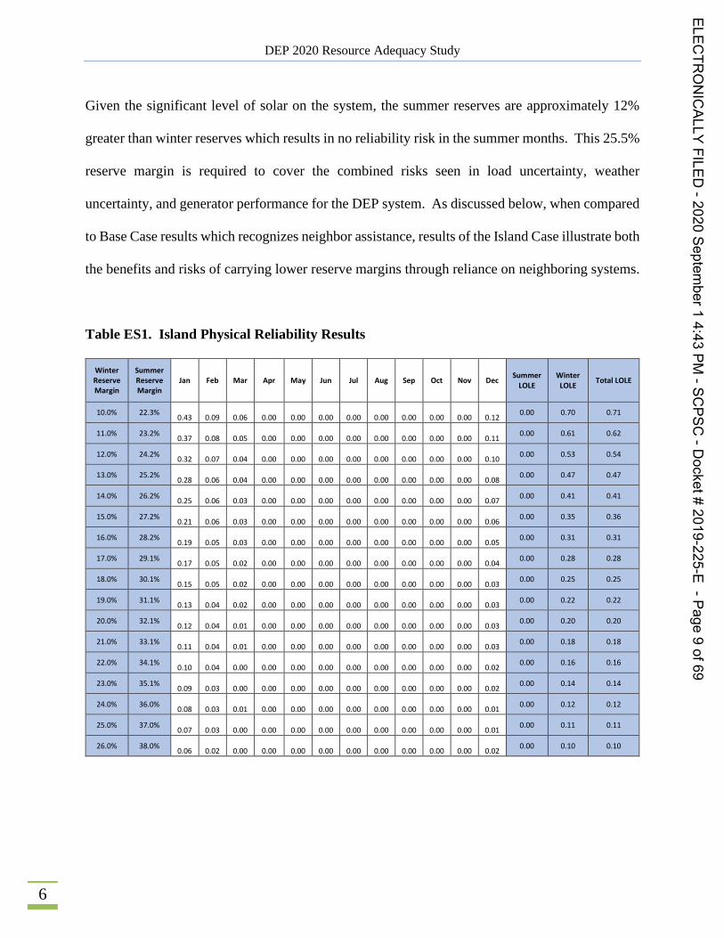
Table ES1 shows the monthly contribution of LOLE at various reserve margin levels for the Island
scenario. In this scenario, it is assumed that DEP is responsible for its own load and that there is
no assistance from neighboring utilities. The summer and winter reserve margins differ for all
scenarios due to seasonal demand forecast differences, weather-related thermal generation
capacity differences, demand response seasonal availability, and seasonal solar capacity value.
Using the one day in 10-year standard (LOLE of 0.1), which is used across the industry to set
minimum target reserve margin levels, DEP would require a 25.5% winter reserve margin in the
Island Case where no assistance from neighboring systems was assumed.
ELECTR
ONICALLY
FILED-2020
September1
4:43PM
-SCPSC
-Docket#
2019-225-E-Page
8of69
DEP 2020 Resource Adequacy Study
6
Given the significant level of solar on the system, the summer reserves are approximately 12%
greater than winter reserves which results in no reliability risk in the summer months. This 25.5%
reserve margin is required to cover the combined risks seen in load uncertainty, weather
uncertainty, and generator performance for the DEP system. As discussed below, when compared
to Base Case results which recognizes neighbor assistance, results of the Island Case illustrate both
the benefits and risks of carrying lower reserve margins through reliance on neighboring systems.
Table ES1. Island Physical Reliability Results
Winter Reserve Margin
Summer Reserve Margin
Jan Feb Mar Apr May Jun Jul Aug Sep Oct Nov Dec Summer LOLE
Winter LOLE Total LOLE
10.0% 22.3% 0.43
0.09
0.06
0.00
0.00
0.00
0.00
0.00
0.00
0.00
0.00
0.12 0.00 0.70 0.71
11.0% 23.2% 0.37
0.08
0.05
0.00
0.00
0.00
0.00
0.00
0.00
0.00
0.00
0.11 0.00 0.61 0.62
12.0% 24.2% 0.32
0.07
0.04
0.00
0.00
0.00
0.00
0.00
0.00
0.00
0.00
0.10 0.00 0.53 0.54
13.0% 25.2% 0.28
0.06
0.04
0.00
0.00
0.00
0.00
0.00
0.00
0.00
0.00
0.08 0.00 0.47 0.47
14.0% 26.2% 0.25
0.06
0.03
0.00
0.00
0.00
0.00
0.00
0.00
0.00
0.00
0.07 0.00 0.41 0.41
15.0% 27.2% 0.21
0.06
0.03
0.00
0.00
0.00
0.00
0.00
0.00
0.00
0.00
0.06 0.00 0.35 0.36
16.0% 28.2% 0.19
0.05
0.03
0.00
0.00
0.00
0.00
0.00
0.00
0.00
0.00
0.05 0.00 0.31 0.31
17.0% 29.1% 0.17
0.05
0.02
0.00
0.00
0.00
0.00
0.00
0.00
0.00
0.00
0.04 0.00 0.28 0.28
18.0% 30.1% 0.15
0.05
0.02
0.00
0.00
0.00
0.00
0.00
0.00
0.00
0.00
0.03 0.00 0.25 0.25
19.0% 31.1% 0.13
0.04
0.02
0.00
0.00
0.00
0.00
0.00
0.00
0.00
0.00
0.03 0.00 0.22 0.22
20.0% 32.1% 0.12
0.04
0.01
0.00
0.00
0.00
0.00
0.00
0.00
0.00
0.00
0.03 0.00 0.20 0.20
21.0% 33.1% 0.11
0.04
0.01
0.00
0.00
0.00
0.00
0.00
0.00
0.00
0.00
0.03 0.00 0.18 0.18
22.0% 34.1% 0.10
0.04
0.00
0.00
0.00
0.00
0.00
0.00
0.00
0.00
0.00
0.02 0.00 0.16 0.16
23.0% 35.1% 0.09
0.03
0.00
0.00
0.00
0.00
0.00
0.00
0.00
0.00
0.00
0.02 0.00 0.14 0.14
24.0% 36.0% 0.08
0.03
0.01
0.00
0.00
0.00
0.00
0.00
0.00
0.00
0.00
0.01 0.00 0.12 0.12
25.0% 37.0% 0.07
0.03
0.00
0.00
0.00
0.00
0.00
0.00
0.00
0.00
0.00
0.01 0.00 0.11 0.11
26.0% 38.0% 0.06
0.02
0.00
0.00
0.00
0.00
0.00
0.00
0.00
0.00
0.00
0.02 0.00 0.10 0.10
ELECTR
ONICALLY
FILED-2020
September1
4:43PM
-SCPSC
-Docket#
2019-225-E-Page
9of69
DEP 2020 Resource Adequacy Study
7
Physical Reliability Results-Base Case
Astrapé recognizes that DEP is part of the larger eastern interconnection and models neighbors
one tie away to allow for market assistance during peak load periods. However, it is important to
also understand that there is risk in relying on neighboring capacity that is less dependable than
owned or contracted generation in which DEP would have first call rights. While there are
certainly advantages of being interconnected due to weather diversity and generator outage
diversity across regions, market assistance is not guaranteed and Astrapé believes Duke Energy
has taken a moderate to aggressive approach (i.e. taking significant credit for neighboring regions)
to modeling neighboring assistance compared to other surrounding entities such as PJM
Interconnection L.L.C. (PJM)5 and the Midcontinent Independent System Operator (MISO)6. A
full description of the market assistance modeling and topology is available in the body of the
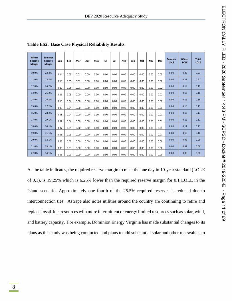
report. Table ES2 shows the monthly LOLE at various reserve margin levels for the Base Case
scenario which is the Island scenario with neighbor assistance included7.
5 PJM limits market assistance to 3,500 MW which represents approximately 2.3% of its reserve margin compared to 6.25% assumed for DEP. https://www.pjm.com/-/media/committees-groups/subcommittees/raas/20191008/20191008-pjm-reserve-requirement-study-draft-2019.ashx – page 11 6MISO limits external assistance to a Unforced Capacity (UCAP) of 2,331 MW which represents approximately 1.8% of its reserve margin compared to 6.25% assumed for DEP. https://www.misoenergy.org/api/documents/getbymediaid/80578 page 24 (copy and paste link in browser) 7 Reference Appendix B, Table B.1 for percentage of loss of load by month and hour of day for the Base Case.
ELECTR
ONICALLY
FILED-2020
September1
4:43PM
-SCPSC
-Docket#
2019-225-E-Page
10of69
DEP 2020 Resource Adequacy Study
8
Table ES2. Base Case Physical Reliability Results
Winter Reserve Margin
Summer Reserve Margin
Jan Feb Mar Apr May Jun Jul Aug Sep Oct Nov Dec Summer LOLE
Winter LOLE
Total LOLE
10.0% 22.3% 0.14
0.05
0.01
0.00
0.00
0.00
0.00
0.00
0.00
0.00
0.00
0.03 0.00 0.23 0.23
11.0% 23.2% 0.13
0.05
0.01
0.00
0.00
0.00
0.00
0.00
0.00
0.00
0.00
0.02 0.00 0.21 0.21
12.0% 24.2% 0.12
0.05
0.01
0.00
0.00
0.00
0.00
0.00
0.00
0.00
0.00
0.02 0.00 0.19 0.19
13.0% 25.2% 0.11
0.05
0.00
0.00
0.00
0.00
0.00
0.00
0.00
0.00
0.00
0.02 0.00 0.18 0.18
14.0% 26.2% 0.10
0.04
0.00
0.00
0.00
0.00
0.00
0.00
0.00
0.00
0.00
0.02 0.00 0.16 0.16
15.0% 27.2% 0.09
0.04
0.00
0.00
0.00
0.00
0.00
0.00
0.00
0.00
0.00
0.01 0.00 0.15 0.15
16.0% 28.2% 0.08
0.04
0.00
0.00
0.00
0.00
0.00
0.00
0.00
0.00
0.00
0.01 0.00 0.13 0.13
17.0% 29.1% 0.07
0.04
0.00
0.00
0.00
0.00
0.00
0.00
0.00
0.00
0.00
0.01 0.00 0.12 0.12
18.0% 30.1% 0.07
0.04
0.00
0.00
0.00
0.00
0.00
0.00
0.00
0.00
0.00
0.01 0.00 0.11 0.11
19.0% 31.1% 0.06
0.03
0.00
0.00
0.00
0.00
0.00
0.00
0.00
0.00
0.00
0.01 0.00 0.10 0.10
20.0% 32.1% 0.06
0.03
0.00
0.00
0.00
0.00
0.00
0.00
0.00
0.00
0.00
0.00 0.00 0.09 0.09
21.0% 33.1% 0.05
0.03
0.00
0.00
0.00
0.00
0.00
0.00
0.00
0.00
0.00
0.00 0.00 0.09 0.09
22.0% 34.1% 0.05
0.03
0.00
0.00
0.00
0.00
0.00
0.00
0.00
0.00
0.00
0.00 0.00 0.08 0.08
As the table indicates, the required reserve margin to meet the one day in 10-year standard (LOLE
of 0.1), is 19.25% which is 6.25% lower than the required reserve margin for 0.1 LOLE in the
Island scenario. Approximately one fourth of the 25.5% required reserves is reduced due to
interconnection ties. Astrapé also notes utilities around the country are continuing to retire and
replace fossil-fuel resources with more intermittent or energy limited resources such as solar, wind,
and battery capacity. For example, Dominion Energy Virginia has made substantial changes to its
plans as this study was being conducted and plans to add substantial solar and other renewables to
ELECTR
ONICALLY
FILED-2020
September1
4:43PM
-SCPSC
-Docket#
2019-225-E-Page
11of69
DEP 2020 Resource Adequacy Study
9
its system that could cause additional winter reliability stress than what is modeled. The below
excerpt is from page 6 of Dominion Energy Virginia’s 2020 IRP8:
In the long term, based on current technology, other challenges will arise from the significant development of intermittent solar resources in all Alternative Plans. For example, based on the nature of solar resources, the Company will have excess capacity in the summer, but not enough capacity in the winter. Based on current technology, the Company would need to meet this winter deficit by either building additional energy storage resources or by buying capacity from the market. In addition, the Company would likely need to import a significant amount of energy during the winter, but would need to export or store significant amounts of energy during the spring and fall.
Additionally, PJM now considers the DOM Zone to be a winter peaking zone where winter peaks
are projected to exceed summer peaks for the forecast period.9 While this is only one example,
these potential changes to surrounding resource mixes may lead to less confidence in market
assistance for the future during early morning winter peak loads. Changes in neighboring system
resource portfolios and load profiles will be an important consideration in future resource adequacy
studies. To the extent historic diversification between DEP and neighboring systems declines, the
historic reliability benefits DEP has experienced from being an interconnected system will also
decline. It is worth nothing that after this study was completed, California experienced rolling
blackouts during extreme weather conditions as the ability to rely on imported power has declined
and has shifted away from dispatchable fossil-fuel resources and put greater reliance on
intermittent resources.10 It is premature to fully ascertain the lessons learned from the California
load shed events. However, it does highlight the fact that as DEP reduces dependence on
8 https://cdn-dominionenergy-prd-001.azureedge.net/-/media/pdfs/global/2020-va-integrated-resource-plan.pdf?la=en&rev=fca793dd8eae4ebea4ee42f5642c9509 9 Dominion Energy Virginia 2020 IRP, at 40. 10 http://www.caiso.com/Documents/ISO-Stage-3-Emergency-Declaration-Lifted-Power-Restored-Statewide.pdf
ELECTR
ONICALLY
FILED-2020
September1
4:43PM
-SCPSC
-Docket#
2019-225-E-Page
12of69
DEP 2020 Resource Adequacy Study
10
dispatchable fossil fuels and increases dependence on intermittent resources, it is important to
ensure it is done in a manner that does not impact reliability to customers.
Physical Reliability Results-DEP/DEC Combined Case
In addition to running the Island and Base Case scenarios, a DEP and DEC Combined Case
scenario was simulated to see the reliability impact of DEP and DEC as a single balancing
authority. In this scenario, DEC and DEP prioritize helping each other over their other external
neighbors but also retain access to external market assistance. The various reserve margin levels
are calculated as the total resources in both DEC and DEP using the combined coincident peak
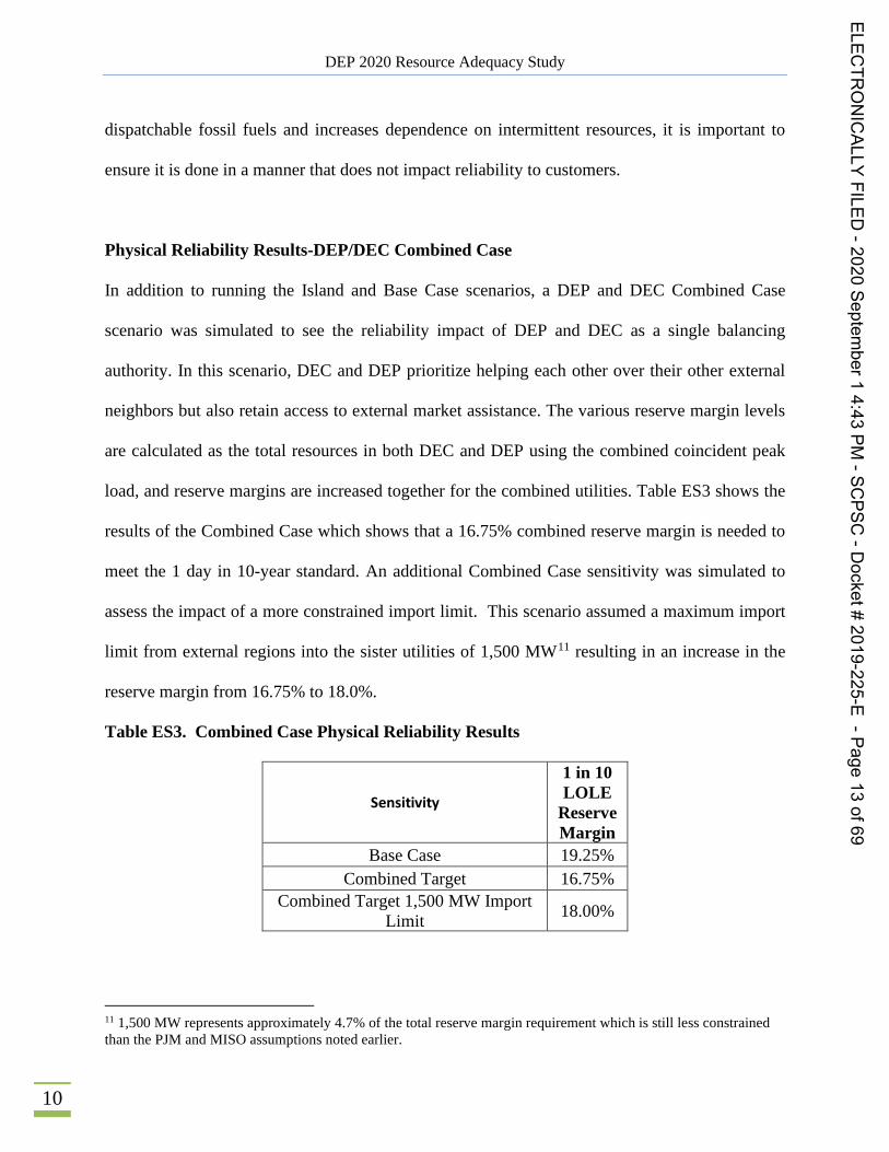
load, and reserve margins are increased together for the combined utilities. Table ES3 shows the
results of the Combined Case which shows that a 16.75% combined reserve margin is needed to
meet the 1 day in 10-year standard. An additional Combined Case sensitivity was simulated to
assess the impact of a more constrained import limit. This scenario assumed a maximum import
limit from external regions into the sister utilities of 1,500 MW11 resulting in an increase in the
reserve margin from 16.75% to 18.0%.
Table ES3. Combined Case Physical Reliability Results
Sensitivity
1 in 10 LOLE
Reserve Margin
Base Case 19.25% Combined Target 16.75%
Combined Target 1,500 MW Import Limit 18.00%
11 1,500 MW represents approximately 4.7% of the total reserve margin requirement which is still less constrained than the PJM and MISO assumptions noted earlier.
ELECTR
ONICALLY
FILED-2020
September1
4:43PM
-SCPSC
-Docket#
2019-225-E-Page
13of69
DEP 2020 Resource Adequacy Study
11
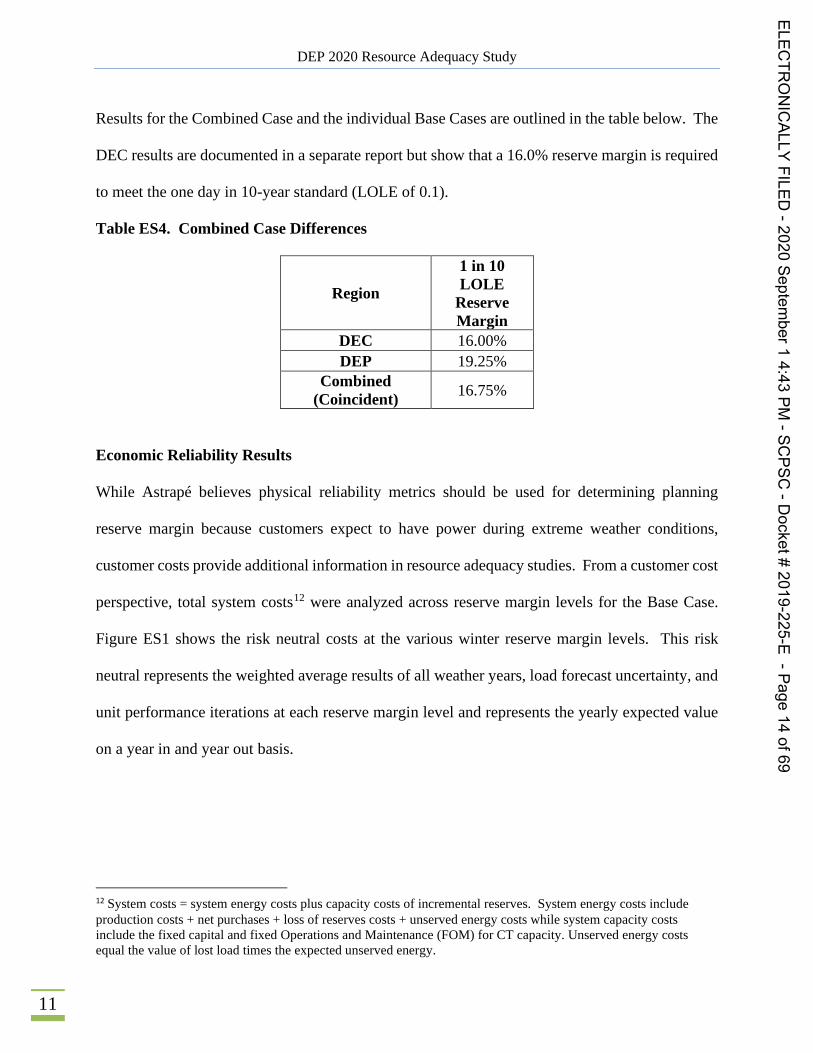
Results for the Combined Case and the individual Base Cases are outlined in the table below. The
DEC results are documented in a separate report but show that a 16.0% reserve margin is required
to meet the one day in 10-year standard (LOLE of 0.1).
Table ES4. Combined Case Differences
Region
1 in 10 LOLE
Reserve Margin
DEC 16.00% DEP 19.25%
Combined (Coincident) 16.75%
Economic Reliability Results
While Astrapé believes physical reliability metrics should be used for determining planning
reserve margin because customers expect to have power during extreme weather conditions,
customer costs provide additional information in resource adequacy studies. From a customer cost
perspective, total system costs12 were analyzed across reserve margin levels for the Base Case.
Figure ES1 shows the risk neutral costs at the various winter reserve margin levels. This risk
neutral represents the weighted average results of all weather years, load forecast uncertainty, and
unit performance iterations at each reserve margin level and represents the yearly expected value
on a year in and year out basis.
12 System costs = system energy costs plus capacity costs of incremental reserves. System energy costs include production costs + net purchases + loss of reserves costs + unserved energy costs while system capacity costs include the fixed capital and fixed Operations and Maintenance (FOM) for CT capacity. Unserved energy costs equal the value of lost load times the expected unserved energy.
ELECTR
ONICALLY
FILED-2020
September1
4:43PM
-SCPSC
-Docket#
2019-225-E-Page
14of69
DEP 2020 Resource Adequacy Study
12
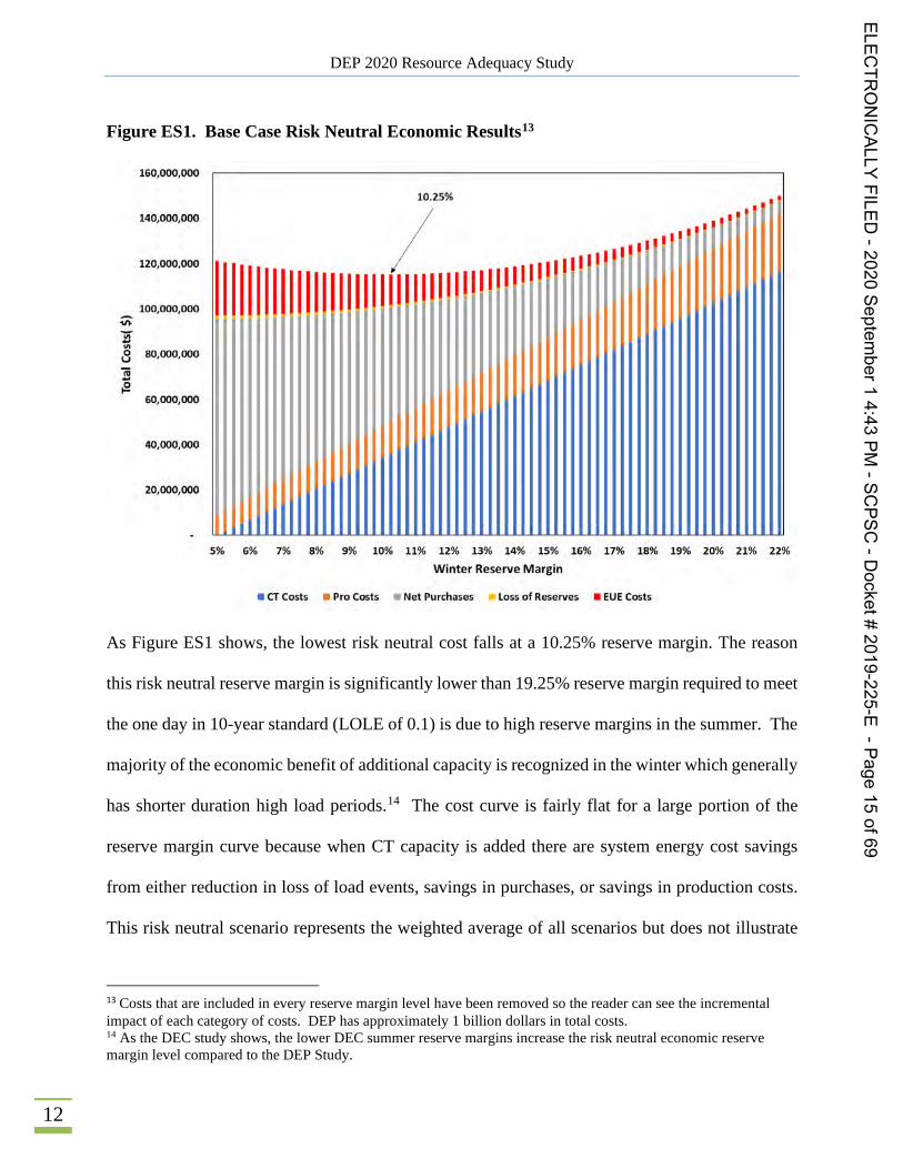
Figure ES1. Base Case Risk Neutral Economic Results13
As Figure ES1 shows, the lowest risk neutral cost falls at a 10.25% reserve margin. The reason
this risk neutral reserve margin is significantly lower than 19.25% reserve margin required to meet
the one day in 10-year standard (LOLE of 0.1) is due to high reserve margins in the summer. The
majority of the economic benefit of additional capacity is recognized in the winter which generally
has shorter duration high load periods.14 The cost curve is fairly flat for a large portion of the
reserve margin curve because when CT capacity is added there are system energy cost savings
from either reduction in loss of load events, savings in purchases, or savings in production costs.
This risk neutral scenario represents the weighted average of all scenarios but does not illustrate
13 Costs that are included in every reserve margin level have been removed so the reader can see the incremental impact of each category of costs. DEP has approximately 1 billion dollars in total costs. 14 As the DEC study shows, the lower DEC summer reserve margins increase the risk neutral economic reserve margin level compared to the DEP Study.
ELECTR
ONICALLY
FILED-2020
September1
4:43PM
-SCPSC
-Docket#
2019-225-E-Page
15of69
160,000,000
140,000,000
120,000,000
100,000,000
80,000,000
060,000,000
40,000,000
20,000,000
596 696 796 896 996 1096 1196 1296 1396 1496 1596 1696 1796 1896 1996 2096 219f 2296
Winter Reserve Margin
~ CT Costs ~ Pro Costs ~ Net Purchases ~ Loss of Reserves ~ EVE Costs
DEP 2020 Resource Adequacy Study
13
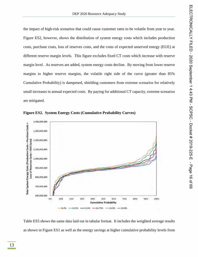
the impact of high-risk scenarios that could cause customer rates to be volatile from year to year.
Figure ES2, however, shows the distribution of system energy costs which includes production
costs, purchase costs, loss of reserves costs, and the costs of expected unserved energy (EUE) at
different reserve margin levels. This figure excludes fixed CT costs which increase with reserve
margin level. As reserves are added, system energy costs decline. By moving from lower reserve
margins to higher reserve margins, the volatile right side of the curve (greater than 85%
Cumulative Probability) is dampened, shielding customers from extreme scenarios for relatively
small increases in annual expected costs. By paying for additional CT capacity, extreme scenarios
are mitigated.
Figure ES2. System Energy Costs (Cumulative Probability Curves)
Table ES5 shows the same data laid out in tabular format. It includes the weighted average results
as shown in Figure ES1 as well as the energy savings at higher cumulative probability levels from
ELECTR
ONICALLY
FILED-2020
September1
4:43PM
-SCPSC
-Docket#
2019-225-E-Page
16of69
+
0Ia0
V
o.+ 0IJ
I0Iv ul0 +
0U0 I
IlIL
Il
ul "0
00 0IuEel
VI
la0
1,400,000,000
1, 300,000,000
1, 200,000,000
1, 100,000,000
1,000,000,000
900,000,000
800,000,000
700,000,000
600,000,00010% 20% 30% 40% 50% 60% 70% 8071 90% 1M%
Cumulative Probability
—8.4% — 10.5% — 12.6% — 14.75'% 16.9% 19.0%
DEP 2020 Resource Adequacy Study
14
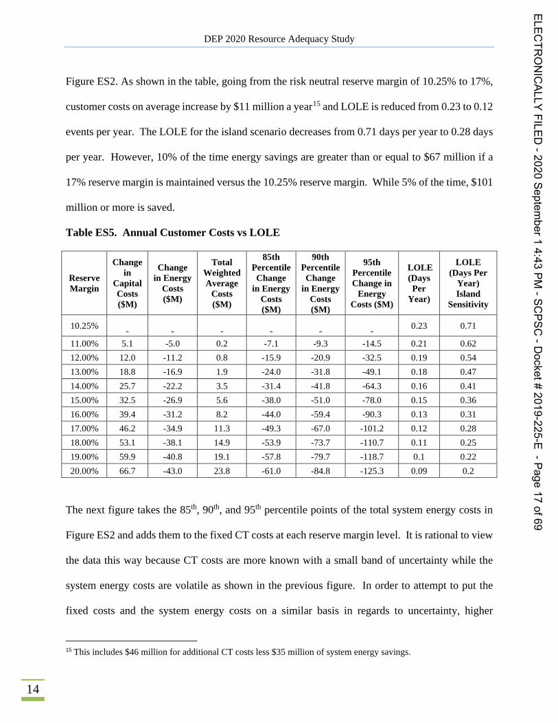
Figure ES2. As shown in the table, going from the risk neutral reserve margin of 10.25% to 17%,
customer costs on average increase by $11 million a year15 and LOLE is reduced from 0.23 to 0.12
events per year. The LOLE for the island scenario decreases from 0.71 days per year to 0.28 days
per year. However, 10% of the time energy savings are greater than or equal to $67 million if a
17% reserve margin is maintained versus the 10.25% reserve margin. While 5% of the time, $101
million or more is saved.
Table ES5. Annual Customer Costs vs LOLE
Reserve Margin
Change in
Capital Costs ($M)
Change in Energy
Costs ($M)
Total Weighted Average
Costs ($M)
85th Percentile Change
in Energy Costs ($M)
90th Percentile
Change in Energy
Costs ($M)
95th Percentile Change in
Energy Costs ($M)
LOLE (Days Per
Year)
LOLE (Days Per
Year) Island
Sensitivity
10.25% -
-
-
-
-
- 0.23 0.71
11.00% 5.1 -5.0 0.2 -7.1 -9.3 -14.5 0.21 0.62 12.00% 12.0 -11.2 0.8 -15.9 -20.9 -32.5 0.19 0.54 13.00% 18.8 -16.9 1.9 -24.0 -31.8 -49.1 0.18 0.47 14.00% 25.7 -22.2 3.5 -31.4 -41.8 -64.3 0.16 0.41 15.00% 32.5 -26.9 5.6 -38.0 -51.0 -78.0 0.15 0.36 16.00% 39.4 -31.2 8.2 -44.0 -59.4 -90.3 0.13 0.31 17.00% 46.2 -34.9 11.3 -49.3 -67.0 -101.2 0.12 0.28 18.00% 53.1 -38.1 14.9 -53.9 -73.7 -110.7 0.11 0.25 19.00% 59.9 -40.8 19.1 -57.8 -79.7 -118.7 0.1 0.22 20.00% 66.7 -43.0 23.8 -61.0 -84.8 -125.3 0.09 0.2
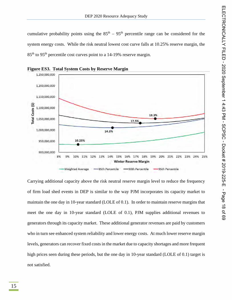
The next figure takes the 85th, 90th, and 95th percentile points of the total system energy costs in
Figure ES2 and adds them to the fixed CT costs at each reserve margin level. It is rational to view
the data this way because CT costs are more known with a small band of uncertainty while the
system energy costs are volatile as shown in the previous figure. In order to attempt to put the
fixed costs and the system energy costs on a similar basis in regards to uncertainty, higher
15 This includes $46 million for additional CT costs less $35 million of system energy savings.
ELECTR
ONICALLY
FILED-2020
September1
4:43PM
-SCPSC
-Docket#
2019-225-E-Page
17of69
DEP 2020 Resource Adequacy Study
15
cumulative probability points using the 85th – 95th percentile range can be considered for the
system energy costs. While the risk neutral lowest cost curve falls at 10.25% reserve margin, the
85th to 95th percentile cost curves point to a 14-19% reserve margin.
Figure ES3. Total System Costs by Reserve Margin
Carrying additional capacity above the risk neutral reserve margin level to reduce the frequency
of firm load shed events in DEP is similar to the way PJM incorporates its capacity market to
maintain the one day in 10-year standard (LOLE of 0.1). In order to maintain reserve margins that
meet the one day in 10-year standard (LOLE of 0.1), PJM supplies additional revenues to
generators through its capacity market. These additional generator revenues are paid by customers
who in turn see enhanced system reliability and lower energy costs. At much lower reserve margin
levels, generators can recover fixed costs in the market due to capacity shortages and more frequent
high prices seen during these periods, but the one day in 10-year standard (LOLE of 0.1) target is
not satisfied.
ELECTR
ONICALLY
FILED-2020
September1
4:43PM
-SCPSC
-Docket#
2019-225-E-Page
18of69
1,250,000,00D
1,200,000,000
1, 150,000,000
1,100,000,000e0V
1,050,000,000ct
1,000,000,DOO
950,000,000
900,000,0006% 9% 10% 11% 12% 13% 14% 15% 16% 17% 1B% 19% 20% 21% 22% 23% 24% 25%
Winter Reserve Margin
—Weighted Average —85th Percentile —90th Percentile 95th Percentile
DEP 2020 Resource Adequacy Study
16
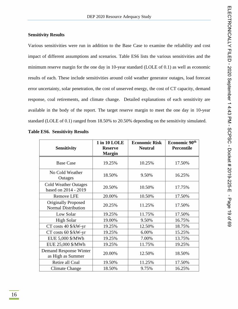
Sensitivity Results
Various sensitivities were run in addition to the Base Case to examine the reliability and cost
impact of different assumptions and scenarios. Table ES6 lists the various sensitivities and the
minimum reserve margin for the one day in 10-year standard (LOLE of 0.1) as well as economic
results of each. These include sensitivities around cold weather generator outages, load forecast
error uncertainty, solar penetration, the cost of unserved energy, the cost of CT capacity, demand
response, coal retirements, and climate change. Detailed explanations of each sensitivity are
available in the body of the report. The target reserve margin to meet the one day in 10-year
standard (LOLE of 0.1) ranged from 18.50% to 20.50% depending on the sensitivity simulated.
Table ES6. Sensitivity Results
Sensitivity 1 in 10 LOLE
Reserve Margin
Economic Risk Neutral
Economic 90th Percentile
Base Case 19.25% 10.25% 17.50%
No Cold Weather Outages 18.50% 9.50% 16.25%
Cold Weather Outages based on 2014 - 2019 20.50% 10.50% 17.75%
Remove LFE 20.00% 10.50% 17.50% Originally Proposed Normal Distribution 20.25% 11.25% 17.50%
Low Solar 19.25% 11.75% 17.50% High Solar 19.00% 9.50% 16.75%
CT costs 40 $/kW-yr 19.25% 12.50% 18.75% CT costs 60 $/kW-yr 19.25% 6.00% 15.25% EUE 5,000 $/MWh 19.25% 7.00% 13.75% EUE 25,000 $/MWh 19.25% 11.75% 19.25%
Demand Response Winter as High as Summer 20.00% 12.50% 18.50%
Retire all Coal 19.50% 11.25% 17.50% Climate Change 18.50% 9.75% 16.25%
ELECTR
ONICALLY
FILED-2020
September1
4:43PM
-SCPSC
-Docket#
2019-225-E-Page
19of69
DEP 2020 Resource Adequacy Study
17
Recommendation
Based on the physical reliability results of the Island, Base Case, Combined Case, additional
sensitivities, as well as the results of the separate DEC Study, Astrapé recommends that DEP
continue to maintain a minimum 17% reserve margin for IRP purposes. This reserve margin
ensures reasonable reliability for customers. Astrapé recognizes that a standalone DEP utility
would require a 25.5% reserve margin to meet the one day in 10-year standard (LOLE of 0.1) and
even with market assistance, DEP would need to maintain a 19.25% reserve margin. Customers
expect electricity during extreme hot and cold weather conditions and maintaining a 17% reserve
margin is estimated to provide an LOLE of 0.12 events per year which is slightly less reliable than
the one day in 10-year standard (LOLE of 0.1). However, given the combined DEC and DEP
sensitivity resulting in a 16.75% reserve margin, and the 16% reserve margin required by DEC to
meet the one day in 10-year standard (LOLE of 0.1), Astrapé believes the 17% reserve margin as
a minimum target is still reasonable for planning purposes. Since the sensitivity results removing
all economic load forecast uncertainty increase the reserve margin to meet the 1 day in 10-year
standard, Astrapé believes this 17% minimum reserve margin should be used in the short- and
long-term planning process.
To be clear, even with 17% reserves, this does not mean that DEP will never be forced to shed
firm load during extreme conditions as DEP and its neighbors shift to reliance on intermittent and
energy limited resources such as storage and demand response. DEP has had several events in the
past few years where actual operating reserves were close to being exhausted even with higher
than 17% planning reserve margins. If not for non-firm external assistance, which this study
considers, firm load would have been shed. In addition, incorporation of tail end reliability risk in
ELECTR
ONICALLY
FILED-2020
September1
4:43PM
-SCPSC
-Docket#
2019-225-E-Page
20of69

DEP 2020 Resource Adequacy Study
18
modeling should be from statistically and historically defendable methods; not from including
subjective risks that cannot be assigned probability. Astrapé’s approach has been to model the
system’s risks around weather, load, generator performance, and market assistance as accurately
as possible without overly conservative assumptions. Based on all results, Astrapé believes
planning to a 17% reserve margin is prudent from a physical reliability perspective and for small
increases in costs above the risk-neutral 10.25% reserve margin level, customers will experience
enhanced reliability and less rate volatility.
As the DEP resource portfolio changes with the addition of more intermittent resources and energy
limited resources, the 17% minimum reserve margin is sufficient as long as the Company has
accounted for the capacity value of solar and battery resources which changes as a function of
penetration. DEP should also monitor changes in the IRPs of neighboring utilities and the potential
impact on market assistance. Unless DEP observes seasonal risk shifting back to summer, the
17% reserve margin should be reasonable but should be re-evaluated as appropriate in future IRPs
and in future reliability studies. To ensure summer reliability is maintained, Astrapé recommends
not allowing the summer reserve margin to drop below 15%.16
16 Currently, if a winter target is maintained at 17%, summer reserves will be above 15%.
ELECTR
ONICALLY
FILED-2020
September1
4:43PM
-SCPSC
-Docket#
2019-225-E-Page
21of69

DEP 2020 Resource Adequacy Study
19
I. List of Figures
Figure 1. Study Topology .......................................................................................................................... 22 Figure 2. DEP Summer Peak Weather Variability..................................................................................... 24 Figure 3. DEP Winter Peak Weather Variability ....................................................................................... 25 Figure 4. DEP Winter Calibration.............................................................................................................. 26 Figure 5. DEP Annual Energy Variability ................................................................................................. 27 Figure 6. Solar Map ................................................................................................................................... 34 Figure 7. Average August Output for Different Inverter Loading Ratios .................................................. 35 Figure 8. Scheduled Capacity .................................................................................................................... 36 Figure 9. Hydro Energy by Weather Year ................................................................................................. 37 Figure 10. Operating Reserve Demand Curve (ORDC) ............................................................................ 40 Figure 11. Base Case Risk Neutral Economic Results .............................................................................. 49 Figure 12. Cumulative Probability Curves ................................................................................................ 51 Figure 13. Total System Costs by Reserve Margin.................................................................................... 53
ELECTR
ONICALLY
FILED-2020
September1
4:43PM
-SCPSC
-Docket#
2019-225-E-Page
22of69
DEP 2020 Resource Adequacy Study
20
II. List of Tables
Table 1. 2024 Forecast: DEP Seasonal Peak (MW) .................................................................................. 23 Table 2. External Region Summer Load Diversity .................................................................................... 28 Table 3. External Region Winter Load Diversity ...................................................................................... 28 Table 4. Load Forecast Error ..................................................................................................................... 29 Table 5. DEP Baseload and Intermediate Resources ................................................................................. 30 Table 6. DEP Peaking Resources ............................................................................................................... 30 Table 7. DEP Renewable Resources Excluding Existing Hydro ............................................................... 33 Table 8. DEP Demand Response Modeling ............................................................................................... 38 Table 9. Unserved Energy Costs / Value of Lost Load .............................................................................. 41 Table 10. Case Probability Example .......................................................................................................... 42 Table 11. Relationship Between Winter and Summer Reserve Margin Levels ......................................... 44 Table 12. Island Physical Reliability Results ............................................................................................. 45 Table 13. Base Case Physical Reliability Results ...................................................................................... 46 Table 14. Reliability Metrics: Base Case ................................................................................................... 48 Table 15. Annual Customer Costs vs LOLE .............................................................................................. 52 Table 16. No Cold Weather Outage Results .............................................................................................. 55 Table 17. Cold Weather Outages Based on 2014-2019 Results ................................................................ 55 Table 18. Remove LFE Results ................................................................................................................. 56 Table 19. Originally Proposed LFE Distribution Results .......................................................................... 56 Table 20. Low Solar Results ...................................................................................................................... 57 Table 21. High Solar Results ..................................................................................................................... 57 Table 22. Demand Response Results ......................................................................................................... 58 Table 23. No Coal Results ......................................................................................................................... 58 Table 24. Climate Change Results ............................................................................................................. 59 Table 25. Economic Sensitivities ............................................................................................................... 60 Table 26. Combined Case Results ............................................................................................................. 61
ELECTR
ONICALLY
FILED-2020
September1
4:43PM
-SCPSC
-Docket#
2019-225-E-Page
23of69
DEP 2020 Resource Adequacy Study
21
III. Input Assumptions
A. Study Year
The selected study year is 202417. The SERVM simulation results are broadly applicable to future
years assuming that resource mixes and market structures do not change in a manner that shifts the
reliability risk to a different season or different time of day.
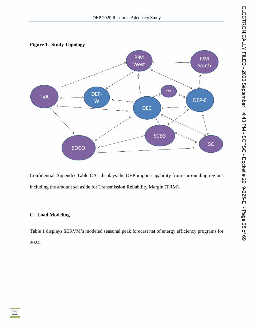
B. Study Topology
Figure 1 shows the study topology that was used for the Resource Adequacy Study. DEP was
modeled in two interconnect zones: (1) DEP – E and (2) DEP – W. While market assistance is not
as dependable as resources that are utility owned or have firm contracts, Astrapé believes it is
appropriate to capture the load diversity and generator outage diversity that DEP has with its
neighbors. For this study, the DEP system was modeled with eight surrounding regions. The
surrounding regions captured in the modeling included Duke Energy Carolinas (DEC), Tennessee
Valley Authority (TVA), Southern Company (SOCO), PJM West & PJM South, Yadkin (YAD),
Dominion Energy South Carolina (formally known as South Carolina Electric & Gas (SCEG)),
and Santee Cooper (SC). SERVM uses a pipe and bubble representation in which energy can be
shared based on economics but subject to transmission constraints.
17 The year 2024 was chosen because it is four years into the future which is indicative of the amount of time needed to permit and construct a new generating facility.
ELECTR
ONICALLY
FILED-2020
September1
4:43PM
-SCPSC
-Docket#
2019-225-E-Page
24of69
DEP 2020 Resource Adequacy Study
22
Figure 1. Study Topology
Confidential Appendix Table CA1 displays the DEP import capability from surrounding regions
including the amount set aside for Transmission Reliability Margin (TRM).
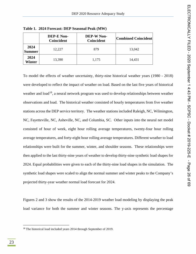
C. Load Modeling
Table 1 displays SERVM’s modeled seasonal peak forecast net of energy efficiency programs for
2024.
ELECTR
ONICALLY
FILED-2020
September1
4:43PM
-SCPSC
-Docket#
2019-225-E-Page
25of69
PJM
'est
PJM
South
~ ~
DEC
YAD
DEP-E,
i soco i
SCEG 'C
DEP 2020 Resource Adequacy Study
23
Table 1. 2024 Forecast: DEP Seasonal Peak (MW)
DEP-E Non- Coincident
DEP-W Non- Coincident Combined Coincident
2024 Summer 12,227 879 13,042
2024 Winter 13,390 1,175 14,431
To model the effects of weather uncertainty, thirty-nine historical weather years (1980 - 2018)
were developed to reflect the impact of weather on load. Based on the last five years of historical
weather and load18, a neural network program was used to develop relationships between weather
observations and load. The historical weather consisted of hourly temperatures from five weather
stations across the DEP service territory. The weather stations included Raleigh, NC, Wilmington,
NC, Fayetteville, NC, Asheville, NC, and Columbia, SC. Other inputs into the neural net model
consisted of hour of week, eight hour rolling average temperatures, twenty-four hour rolling
average temperatures, and forty-eight hour rolling average temperatures. Different weather to load
relationships were built for the summer, winter, and shoulder seasons. These relationships were
then applied to the last thirty-nine years of weather to develop thirty-nine synthetic load shapes for
2024. Equal probabilities were given to each of the thirty-nine load shapes in the simulation. The
synthetic load shapes were scaled to align the normal summer and winter peaks to the Company’s
projected thirty-year weather normal load forecast for 2024.
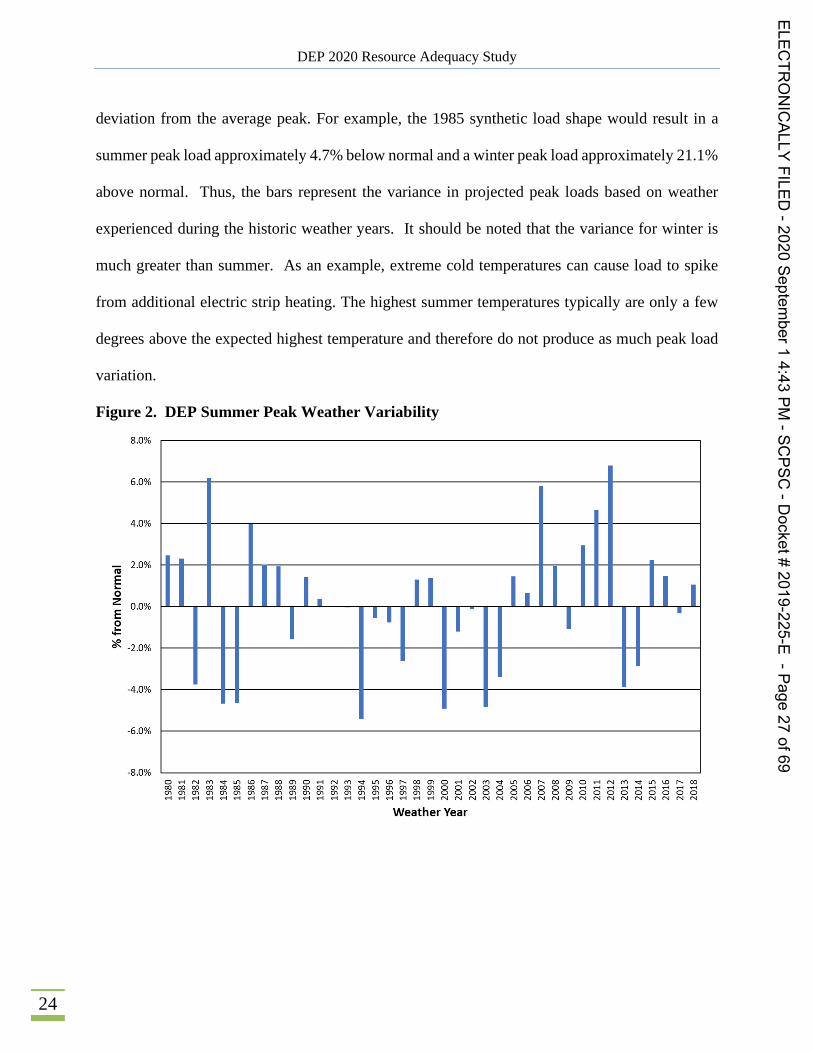
Figures 2 and 3 show the results of the 2014-2019 weather load modeling by displaying the peak
load variance for both the summer and winter seasons. The y-axis represents the percentage
18 The historical load included years 2014 through September of 2019.
ELECTR
ONICALLY
FILED-2020
September1
4:43PM
-SCPSC
-Docket#
2019-225-E-Page
26of69
DEP 2020 Resource Adequacy Study
24
deviation from the average peak. For example, the 1985 synthetic load shape would result in a
summer peak load approximately 4.7% below normal and a winter peak load approximately 21.1%
above normal. Thus, the bars represent the variance in projected peak loads based on weather
experienced during the historic weather years. It should be noted that the variance for winter is
much greater than summer. As an example, extreme cold temperatures can cause load to spike
from additional electric strip heating. The highest summer temperatures typically are only a few
degrees above the expected highest temperature and therefore do not produce as much peak load
variation.
Figure 2. DEP Summer Peak Weather Variability
ELECTR
ONICALLY
FILED-2020
September1
4:43PM
-SCPSC
-Docket#
2019-225-E-Page
27of69
2.096
E0+ o.oxE0
@ -2.0%
-4.0%
-6.0%
-8.0%ClCO CO CO CO CO CO CO CO CO CO Ol (O Ol Ol O Ol CO Ol Ol 0 0 O 0 O O O O 0 O 00 Ol 0 O 0 0 0 (h Ol 0 0 0 0 Ol 0 Ol 0 0 Ol 0 0 0 0 0 0 0 0 0 0 0 0 0 0 0 0 0 0 0 0
CC C( OI I I CC C( I C( I CC I CC I OI C( OI CC
Weather Year
DEP 2020 Resource Adequacy Study
25
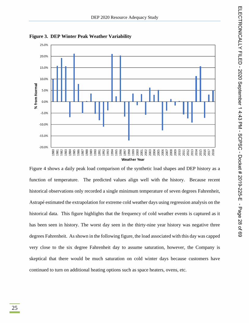
Figure 3. DEP Winter Peak Weather Variability
Figure 4 shows a daily peak load comparison of the synthetic load shapes and DEP history as a
function of temperature. The predicted values align well with the history. Because recent
historical observations only recorded a single minimum temperature of seven degrees Fahrenheit,
Astrapé estimated the extrapolation for extreme cold weather days using regression analysis on the
historical data. This figure highlights that the frequency of cold weather events is captured as it
has been seen in history. The worst day seen in the thirty-nine year history was negative three
degrees Fahrenheit. As shown in the following figure, the load associated with this day was capped
very close to the six degree Fahrenheit day to assume saturation, however, the Company is
skeptical that there would be much saturation on cold winter days because customers have
continued to turn on additional heating options such as space heaters, ovens, etc.
ELECTR
ONICALLY
FILED-2020
September1
4:43PM
-SCPSC
-Docket#
2019-225-E-Page
28of69
25.0%
20.0%
15.0%
10.0%
5.0%
ZE
0.0%
g-5.0%
-10.0%
-15.0%
-20.0%0 m m m m 0 I m 0 0 m m m 0 I 0 a 0 m m m 0 I «I 0 0 m m m m 0 I «Ico co co co co co co co a\ co al co 0 al m al al m co al 0 0 0 0 0 0 0 0 0 0a Ol 0 0 O al 0 O 0 a O 0 a 0 0 a 0 0 a 0 0 0 0 0 0 0 0 0 0 0 0 0 0 0 0 0 0 0 0cl OI ca ca OI ca ca OI al ca cl al ca cl al ca cl al ca
Weather Year

DEP 2020 Resource Adequacy Study
26
Figure 4. DEP Winter Calibration
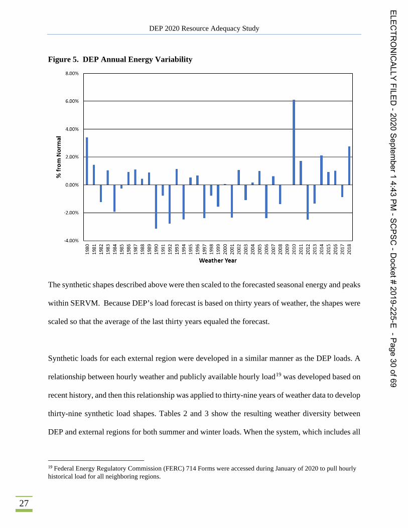
The energy variation is lower than peak variation across the weather years as expected. As shown
in Figure 5, 2010 was an extreme year in total energy due to persistent severe temperatures across
the summer and yet the deviation from average was only 6%.
ELECTR
ONICALLY
FILED-2020
September1
4:43PM
-SCPSC
-Docket#
2019-225-E-Page
29of69
19,5DD
17,500
15,500
13,500
O11,500
te
2'I 9,500tn
7,500
5,500
3,500-5 1D
Dally Min Temperature(ep)
Synthetic ~ DEP Htstottcet
15 20 25
DEP 2020 Resource Adequacy Study
27
Figure 5. DEP Annual Energy Variability
The synthetic shapes described above were then scaled to the forecasted seasonal energy and peaks
within SERVM. Because DEP’s load forecast is based on thirty years of weather, the shapes were
scaled so that the average of the last thirty years equaled the forecast.
Synthetic loads for each external region were developed in a similar manner as the DEP loads. A
relationship between hourly weather and publicly available hourly load19 was developed based on
recent history, and then this relationship was applied to thirty-nine years of weather data to develop
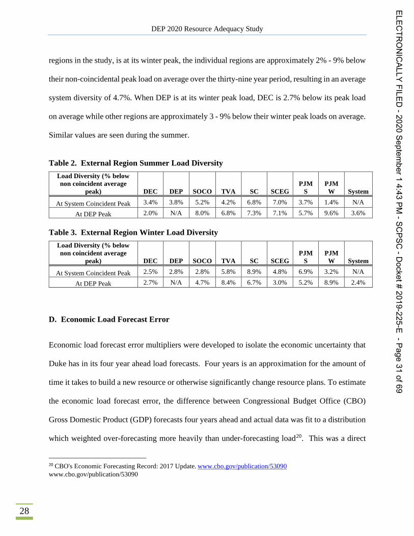
thirty-nine synthetic load shapes. Tables 2 and 3 show the resulting weather diversity between
DEP and external regions for both summer and winter loads. When the system, which includes all
19 Federal Energy Regulatory Commission (FERC) 714 Forms were accessed during January of 2020 to pull hourly historical load for all neighboring regions.
ELECTR
ONICALLY
FILED-2020
September1
4:43PM
-SCPSC
-Docket#
2019-225-E-Page
30of69
8.00%
6.00%
4.00%
E0Z 2.00%E0
g0.00%
-2.00%
-4.00%0 m m m 0 I m 0 0 m m m m 0 I 0 a 0 m m m 0 I «I 0 0 m m m m 0 I «Ico co co co co co co co co co al co a al 0 al al 0 co al 0 0 0 0 0 0 0 0 0 00 0 a 0 0 0 O Ol 0 0 O al a O 0 a 0 0 a 0 0 0 0 0 0 0 0 0 0 0 0 0 0 0 0 0 0 0 0cl OI ca cl OI ca cl ol ol cl cl ol ca cl OI ca cl OI ca
Weather Year
DEP 2020 Resource Adequacy Study
28
regions in the study, is at its winter peak, the individual regions are approximately 2% - 9% below
their non-coincidental peak load on average over the thirty-nine year period, resulting in an average
system diversity of 4.7%. When DEP is at its winter peak load, DEC is 2.7% below its peak load
on average while other regions are approximately 3 - 9% below their winter peak loads on average.
Similar values are seen during the summer.
Table 2. External Region Summer Load Diversity
Load Diversity (% below non coincident average
peak) DEC DEP SOCO TVA SC SCEG PJM
S PJM
W System
At System Coincident Peak 3.4% 3.8% 5.2% 4.2% 6.8% 7.0% 3.7% 1.4% N/A
At DEP Peak 2.0% N/A 8.0% 6.8% 7.3% 7.1% 5.7% 9.6% 3.6% Table 3. External Region Winter Load Diversity
Load Diversity (% below non coincident average
peak) DEC DEP SOCO TVA SC SCEG PJM
S PJM
W System
At System Coincident Peak 2.5% 2.8% 2.8% 5.8% 8.9% 4.8% 6.9% 3.2% N/A
At DEP Peak 2.7% N/A 4.7% 8.4% 6.7% 3.0% 5.2% 8.9% 2.4%
D. Economic Load Forecast Error
Economic load forecast error multipliers were developed to isolate the economic uncertainty that
Duke has in its four year ahead load forecasts. Four years is an approximation for the amount of
time it takes to build a new resource or otherwise significantly change resource plans. To estimate
the economic load forecast error, the difference between Congressional Budget Office (CBO)
Gross Domestic Product (GDP) forecasts four years ahead and actual data was fit to a distribution
which weighted over-forecasting more heavily than under-forecasting load20. This was a direct
20 CBO's Economic Forecasting Record: 2017 Update. www.cbo.gov/publication/53090 www.cbo.gov/publication/53090
ELECTR
ONICALLY
FILED-2020
September1
4:43PM
-SCPSC
-Docket#
2019-225-E-Page
31of69
DEP 2020 Resource Adequacy Study
29
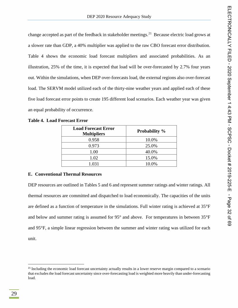
change accepted as part of the feedback in stakeholder meetings.21 Because electric load grows at
a slower rate than GDP, a 40% multiplier was applied to the raw CBO forecast error distribution.
Table 4 shows the economic load forecast multipliers and associated probabilities. As an
illustration, 25% of the time, it is expected that load will be over-forecasted by 2.7% four years
out. Within the simulations, when DEP over-forecasts load, the external regions also over-forecast
load. The SERVM model utilized each of the thirty-nine weather years and applied each of these
five load forecast error points to create 195 different load scenarios. Each weather year was given
an equal probability of occurrence.
Table 4. Load Forecast Error
Load Forecast Error Multipliers Probability %
0.958 10.0% 0.973 25.0% 1.00 40.0% 1.02 15.0% 1.031 10.0%
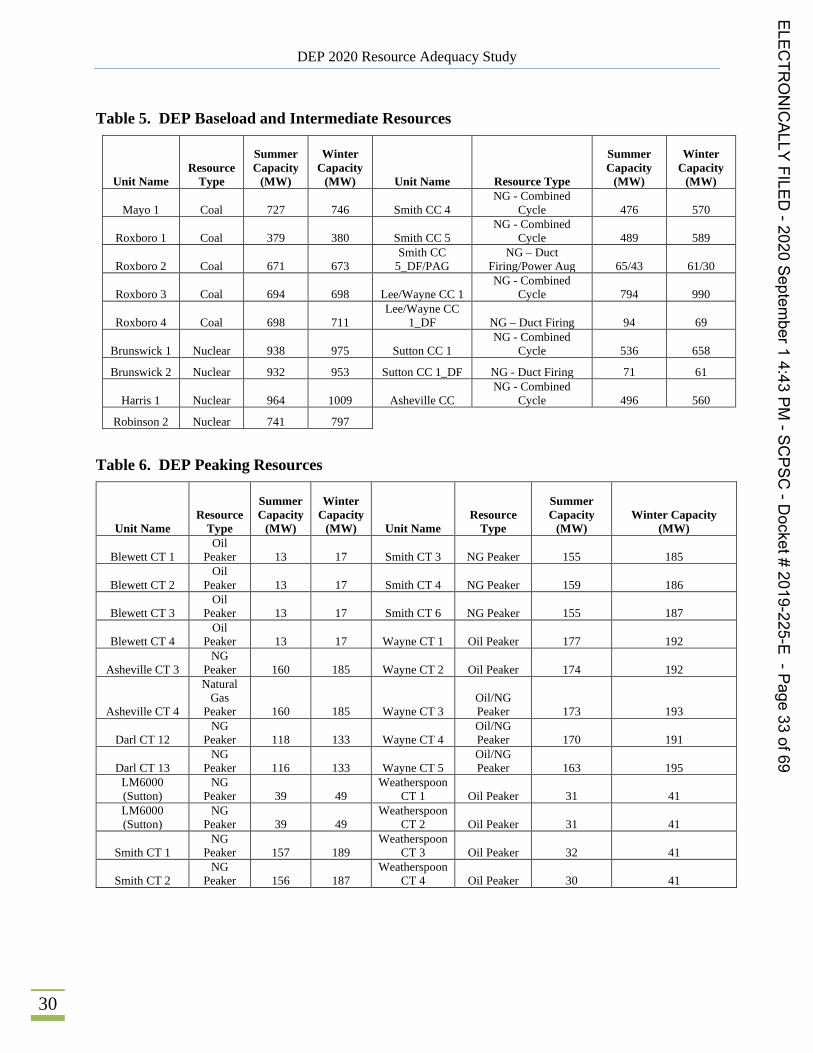
E. Conventional Thermal Resources
DEP resources are outlined in Tables 5 and 6 and represent summer ratings and winter ratings. All
thermal resources are committed and dispatched to load economically. The capacities of the units
are defined as a function of temperature in the simulations. Full winter rating is achieved at 35°F
and below and summer rating is assumed for 95° and above. For temperatures in between 35°F
and 95°F, a simple linear regression between the summer and winter rating was utilized for each
unit.
21 Including the economic load forecast uncertainty actually results in a lower reserve margin compared to a scenario that excludes the load forecast uncertainty since over-forecasting load is weighted more heavily than under-forecasting load.
ELECTR
ONICALLY
FILED-2020
September1
4:43PM
-SCPSC
-Docket#
2019-225-E-Page
32of69
DEP 2020 Resource Adequacy Study
30
Table 5. DEP Baseload and Intermediate Resources
Unit Name Resource
Type
Summer Capacity
(MW)
Winter Capacity
(MW) Unit Name Resource Type
Summer Capacity
(MW)
Winter Capacity
(MW)
Mayo 1 Coal 727 746 Smith CC 4 NG - Combined
Cycle 476 570
Roxboro 1 Coal 379 380 Smith CC 5 NG - Combined
Cycle 489 589
Roxboro 2 Coal 671 673 Smith CC
5_DF/PAG NG – Duct
Firing/Power Aug 65/43 61/30
Roxboro 3 Coal 694 698 Lee/Wayne CC 1 NG - Combined
Cycle 794 990
Roxboro 4 Coal 698 711 Lee/Wayne CC
1_DF NG – Duct Firing 94 69
Brunswick 1 Nuclear 938 975 Sutton CC 1 NG - Combined
Cycle 536 658
Brunswick 2 Nuclear 932 953 Sutton CC 1_DF NG - Duct Firing 71 61
Harris 1 Nuclear 964 1009 Asheville CC NG - Combined
Cycle 496 560
Robinson 2 Nuclear 741 797 Table 6. DEP Peaking Resources
Unit Name Resource
Type
Summer Capacity
(MW)
Winter Capacity
(MW) Unit Name Resource
Type
Summer Capacity
(MW) Winter Capacity
(MW)
Blewett CT 1 Oil
Peaker 13 17 Smith CT 3 NG Peaker 155 185
Blewett CT 2 Oil
Peaker 13 17 Smith CT 4 NG Peaker 159 186
Blewett CT 3 Oil
Peaker 13 17 Smith CT 6 NG Peaker 155 187
Blewett CT 4 Oil
Peaker 13 17 Wayne CT 1 Oil Peaker 177 192
Asheville CT 3 NG
Peaker 160 185 Wayne CT 2 Oil Peaker 174 192
Asheville CT 4
Natural Gas
Peaker 160 185 Wayne CT 3 Oil/NG Peaker 173 193
Darl CT 12 NG
Peaker 118 133 Wayne CT 4 Oil/NG Peaker 170 191
Darl CT 13 NG
Peaker 116 133 Wayne CT 5 Oil/NG Peaker 163 195
LM6000 (Sutton)
NG Peaker 39 49
Weatherspoon CT 1 Oil Peaker 31 41
LM6000 (Sutton)
NG Peaker 39 49
Weatherspoon CT 2 Oil Peaker 31 41
Smith CT 1 NG
Peaker 157 189 Weatherspoon
CT 3 Oil Peaker 32 41
Smith CT 2 NG
Peaker 156 187 Weatherspoon
CT 4 Oil Peaker 30 41
ELECTR
ONICALLY
FILED-2020
September1
4:43PM
-SCPSC
-Docket#
2019-225-E-Page
33of69
DEP 2020 Resource Adequacy Study
31
DEP purchase contracts were modeled as shown in Confidential Appendix Table CA2. These
resources were treated as traditional thermal resources and counted towards reserve margin.
Confidential Appendix Table CA3 shows the fuel prices used in the study for DEP and its
neighboring power systems.
F. Unit Outage Data
Unlike typical production cost models, SERVM does not use an Equivalent Forced Outage Rate
(EFOR) for each unit as an input. Instead, historical Generating Availability Data System (GADS)
data events for the period 2014-2019 are entered in for each unit and SERVM randomly draws
from these events to simulate the unit outages. Units without historical data use history from
similar technologies. The events are entered using the following variables:
Full Outage Modeling Time-to-Repair Hours Time-to-Fail Hours Partial Outage Modeling Partial Outage Time-to-Repair Hours Partial Outage Derate Percentage Partial Outage Time-to-Fail Hours Maintenance Outages Maintenance Outage Rate - % of time in a month that the unit will be on maintenance outage. SERVM uses this percentage and schedules the maintenance outages during off peak periods. Planned Outages The actual schedule for 2024 was used.
To illustrate the outage logic, assume that from 2014 – 2019, a generator had 15 full outage events
and 30 partial outage events reported in the GADS data. The Time-to-Repair and Time-to-Fail
between each event is calculated from the GADS data. These multiple Time-to-Repair and Time-
ELECTR
ONICALLY
FILED-2020
September1
4:43PM
-SCPSC
-Docket#
2019-225-E-Page
34of69
DEP 2020 Resource Adequacy Study
32
to-Fail inputs are the distributions used by SERVM. Because there may be seasonal variances in
EFOR, the data is broken up into seasons such that there is a set of Time-to-Repair and Time-to-
Fail inputs for summer, shoulder, and winter, based on history. Further, assume the generator is
online in hour 1 of the simulation. SERVM will randomly draw both a full outage and partial
outage Time-to-Fail value from the distributions provided. Once the unit has been economically
dispatched for that amount of time, it will fail. A partial outage will be triggered first if the
selected Time-to-Fail value is lower than the selected full outage Time-to-Fail value. Next, the
model will draw a Time-to-Repair value from the distribution and be on outage for that number of
hours. When the repair is complete it will draw a new Time-to-Fail value. The process repeats until
the end of the iteration when it will begin again for the subsequent iteration. The full outage
counters and partial outage counters run in parallel. This more detailed modeling is important to
capture the tails of the distribution that a simple convolution method would not capture.
Confidential Appendix Table CA4 shows system peak season Equivalent Forced Outage Rate
(EFOR) for the system and by unit.
The most important aspect of unit performance modeling in resource adequacy studies is the
cumulative MW offline distribution. Most service reliability problems are due to significant
coincident outages. Confidential Appendix Figure CA1 shows the distribution of modeled system
outages as a percentage of time modeled and compared well with actual historical data.
Additional analysis was performed to understand the impact cold temperatures have on system
outages. Confidential Appendix Figures CA2 and CA3 show the difference in cold weather
outages during the 2014-2019 period and the 2016-2019 period. The 2014-2019 period showed
ELECTR
ONICALLY
FILED-2020
September1
4:43PM
-SCPSC
-Docket#
2019-225-E-Page
35of69

DEP 2020 Resource Adequacy Study
33
more events than the 2016-2019 period which is logical because Duke Energy has put practices in
place to enhance reliability during these periods, however the 2016 – 2019 data shows some events
still occur. The average capacity offline below 10 degrees for DEC and DEP combined was 400
MW. Astrapé split this value by peak load ratio and included 140 MW in the DEP Study and 260
MW in the DEC Study at temperatures below 10 degrees. Sensitivities were performed with the
cold weather outages removed and increased to match the 2014 – 2019 dataset which showed an
average of 800 MW offline on days below 10 degrees. The MWs offline during the 10 coldest days
can be seen in Confidential Appendix Table CA5. The outages shown are only events that included
some type of freezing or cold weather problem as part of the description in the outage event.
G. Solar and Battery Modeling
Table 7 shows the solar and battery resources captured in the study.
Table 7. DEP Renewable Resources Excluding Existing Hydro
Unit Type
Summer Capacity
(MW)
Winter Capacity (MW)
Modeling
Utility Owned-Fixed 141 141 Hourly Profiles
Transition-Fixed 2,432 2,432 Hourly Profiles
Competitive Procurement of Renewable Energy
(CPRE) Tranche 1
Fixed 40%/Tracking 60% 86 86 Hourly Profiles
Future Solar
Fixed 40%/Tracking 60% 1,448 1,448 Hourly Profiles
Total Solar 4,107 4,107
Total Battery 83 83 Modeled as energy arbitrage
ELECTR
ONICALLY
FILED-2020
September1
4:43PM
-SCPSC
-Docket#
2019-225-E-Page
36of69
DEP 2020 Resource Adequacy Study
34
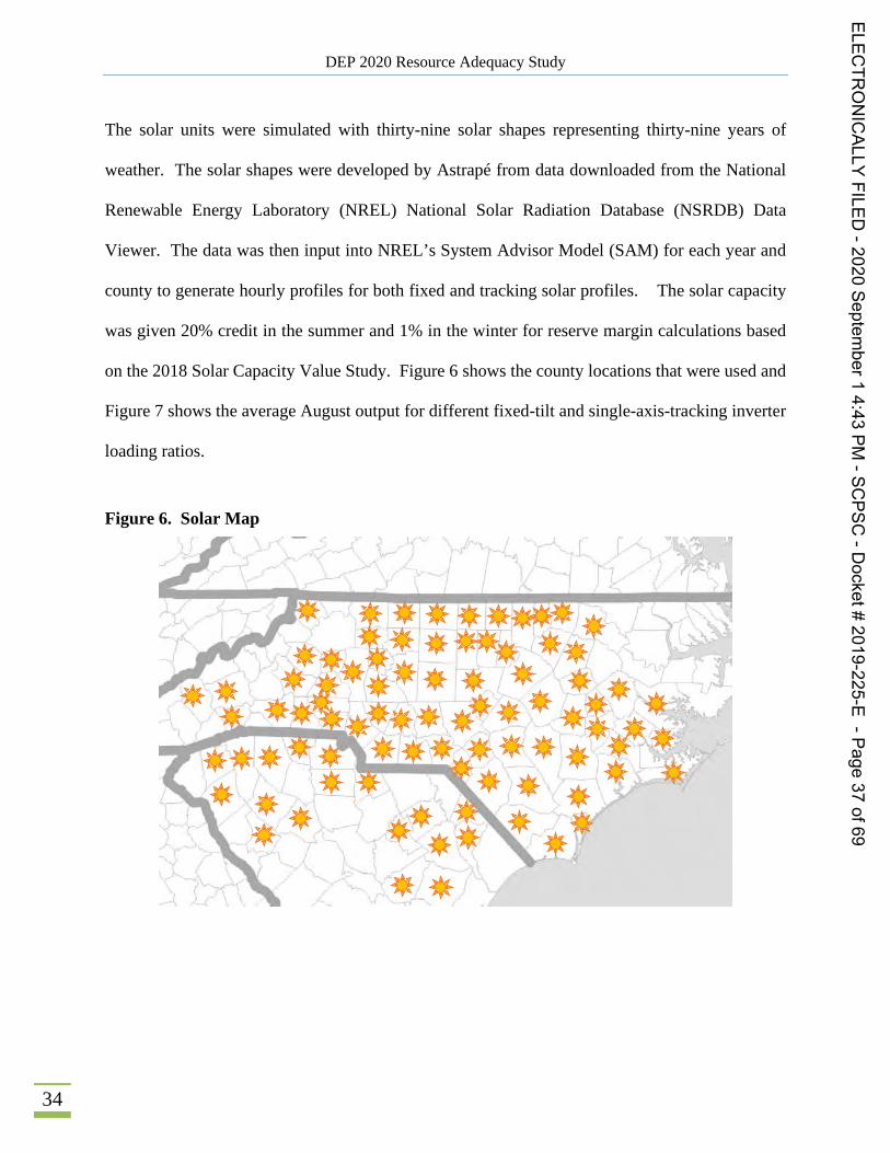
The solar units were simulated with thirty-nine solar shapes representing thirty-nine years of
weather. The solar shapes were developed by Astrapé from data downloaded from the National
Renewable Energy Laboratory (NREL) National Solar Radiation Database (NSRDB) Data
Viewer. The data was then input into NREL’s System Advisor Model (SAM) for each year and
county to generate hourly profiles for both fixed and tracking solar profiles. The solar capacity
was given 20% credit in the summer and 1% in the winter for reserve margin calculations based
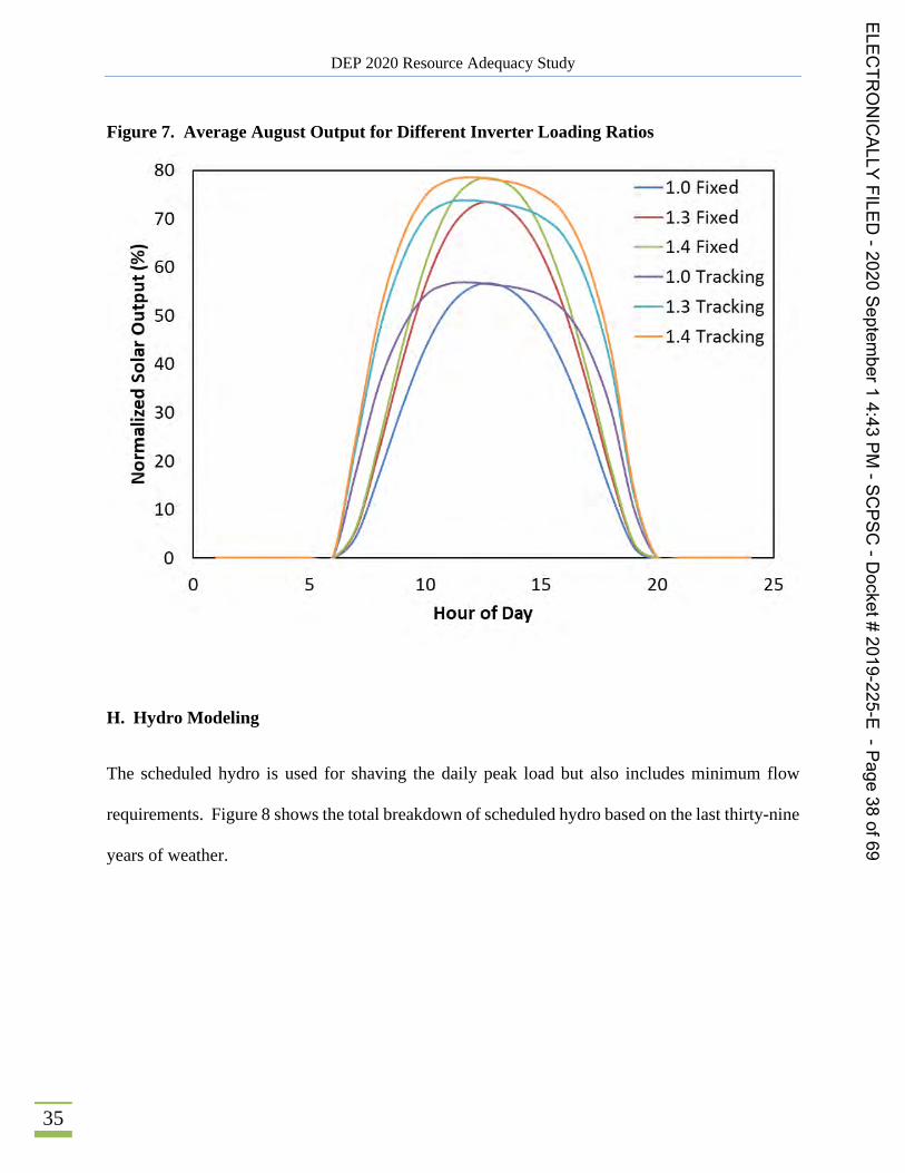
on the 2018 Solar Capacity Value Study. Figure 6 shows the county locations that were used and
Figure 7 shows the average August output for different fixed-tilt and single-axis-tracking inverter
loading ratios.
Figure 6. Solar Map
ELECTR
ONICALLY
FILED-2020
September1
4:43PM
-SCPSC
-Docket#
2019-225-E-Page
37of69
DEP 2020 Resource Adequacy Study
35
Figure 7. Average August Output for Different Inverter Loading Ratios
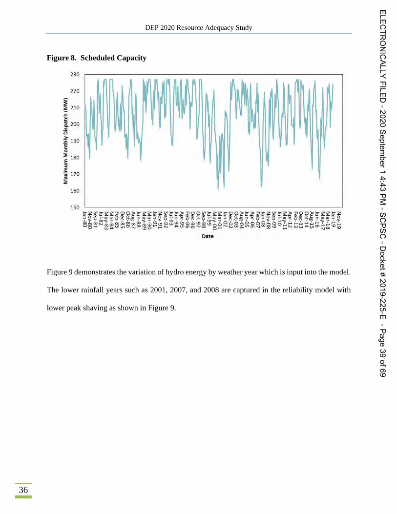
H. Hydro Modeling
The scheduled hydro is used for shaving the daily peak load but also includes minimum flow
requirements. Figure 8 shows the total breakdown of scheduled hydro based on the last thirty-nine
years of weather.
ELECTR
ONICALLY
FILED-2020
September1
4:43PM
-SCPSC
-Docket#
2019-225-E-Page
38of69
80
70
— 60
5 500
o 40Ill
.~ 30
Eo 20Z
10
10 15 20 25
Hour of Day
DEP 2020 Resource Adequacy Study
36
Figure 8. Scheduled Capacity
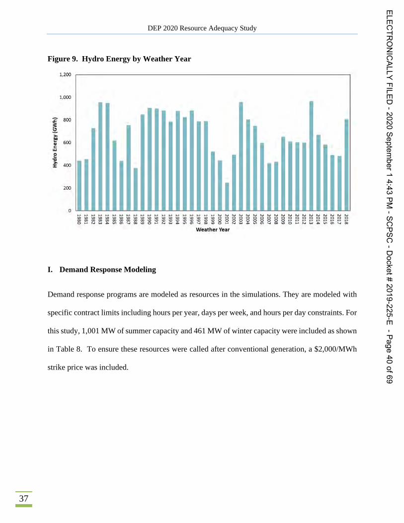
Figure 9 demonstrates the variation of hydro energy by weather year which is input into the model.
The lower rainfall years such as 2001, 2007, and 2008 are captured in the reliability model with
lower peak shaving as shown in Figure 9.
ELECTR
ONICALLY
FILED-2020
September1
4:43PM
-SCPSC
-Docket#
2019-225-E-Page
39of69
230
220
5 210
U
ca 200
0~ 190c0
180E
'x 170
160
150a &De c ZS e~00&c EE a Z Dec c & i~ 0 0 sec ZZ cu 00&c & a~a Z gc 2& a~00&c EZ cu Z
D — oc fDhcDUDDD —D'0 oh — UocfDhcceco — Dao hhcco(DQcococoN 'ocococococo 'ee eluee eooloee 'o00000000 00 ~l'' o I0V eeaaCOCOCOVCOCO0 ~CO DeSCOVCO 0 h OUCUOONCOVCOCoe VNCUul4 IPCO~+gee
Date
DEP 2020 Resource Adequacy Study
37
Figure 9. Hydro Energy by Weather Year
I. Demand Response Modeling
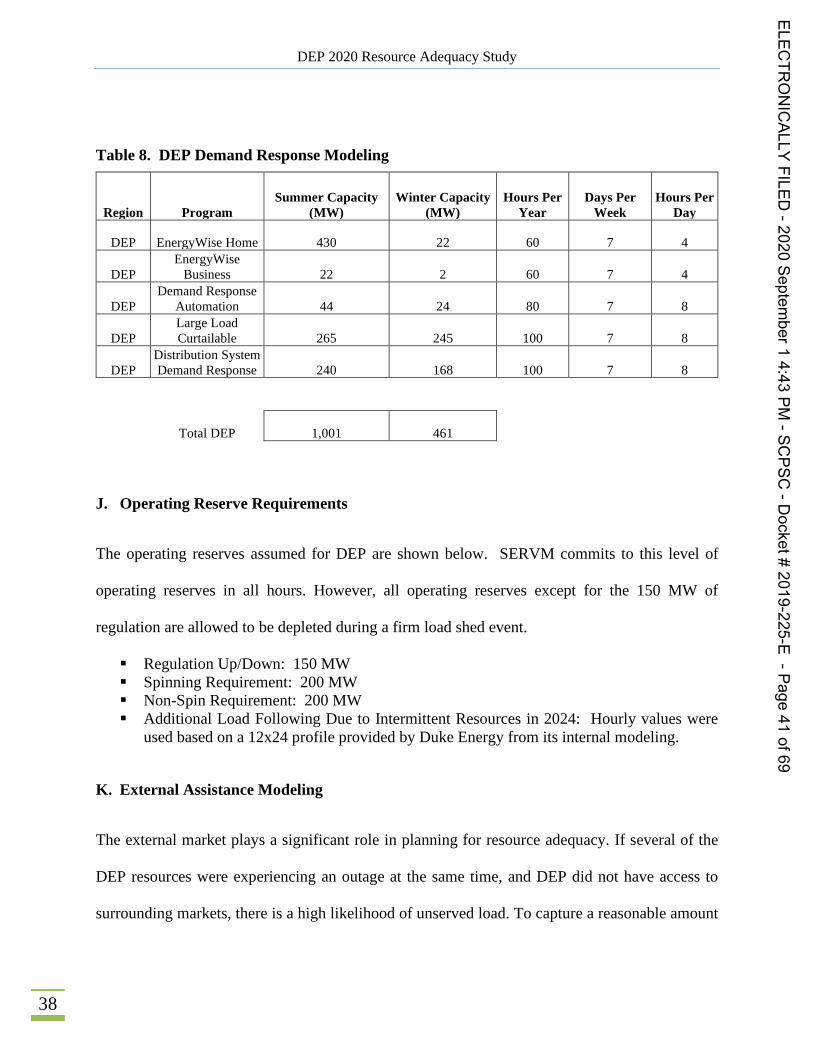
Demand response programs are modeled as resources in the simulations. They are modeled with
specific contract limits including hours per year, days per week, and hours per day constraints. For
this study, 1,001 MW of summer capacity and 461 MW of winter capacity were included as shown
in Table 8. To ensure these resources were called after conventional generation, a $2,000/MWh
strike price was included.
ELECTR
ONICALLY
FILED-2020
September1
4:43PM
-SCPSC
-Docket#
2019-225-E-Page
40of69
1,200
1,000
800
IO600
0IO0
z Coo
0 0 I I R R R t I t 0 0 0 tt II 4 tt 4 4 IO I 0 0 tt tt tt 4 I 4 IJ IOl D ID IO IO D Ul Ol O\ Ol IO ID Ol Ol Cl IO ID IO Ol II Q lj 8 8 Cj I3 8 I3 P 8 CI CI CI CI CI It 0 Cl 00 X 0 4 ID 4 0 N I 6 0 4 I Ot le 6 0 I 4 0 6 0 V I
Weather Year
DEP 2020 Resource Adequacy Study
38
Table 8. DEP Demand Response Modeling
Region Program Summer Capacity
(MW) Winter Capacity
(MW) Hours Per
Year Days Per
Week Hours Per
Day
DEP EnergyWise Home 430 22 60 7 4
DEP EnergyWise
Business 22 2 60 7 4
DEP Demand Response
Automation 44 24 80 7 8
DEP Large Load Curtailable 265 245 100 7 8
DEP Distribution System Demand Response 240 168 100 7 8
Total DEP 1,001 461
J. Operating Reserve Requirements
The operating reserves assumed for DEP are shown below. SERVM commits to this level of
operating reserves in all hours. However, all operating reserves except for the 150 MW of
regulation are allowed to be depleted during a firm load shed event.
Regulation Up/Down: 150 MW Spinning Requirement: 200 MW Non-Spin Requirement: 200 MW Additional Load Following Due to Intermittent Resources in 2024: Hourly values were
used based on a 12x24 profile provided by Duke Energy from its internal modeling.
K. External Assistance Modeling
The external market plays a significant role in planning for resource adequacy. If several of the
DEP resources were experiencing an outage at the same time, and DEP did not have access to
surrounding markets, there is a high likelihood of unserved load. To capture a reasonable amount
ELECTR
ONICALLY
FILED-2020
September1
4:43PM
-SCPSC
-Docket#
2019-225-E-Page
41of69
DEP 2020 Resource Adequacy Study
39
of assistance from surrounding neighbors, each neighbor was modeled at the one day in 10-year
standard (LOLE of 0.1) level representing the target for many entities. By modeling in this manner,
only weather diversity and generator outage diversity benefits are captured. The market
representation used in SERVM is based on Astrapé’s proprietary dataset which is developed based
on FERC Forms, Energy Information Administration (EIA) Forms, and reviews of IRP
information from neighboring regions. To ensure purchases in the model compared well in
magnitude to historical data, the years 2015 and 2018 were simulated since they reflected cold
weather years with high winter peaks. Figure CA4 in the confidential appendix shows that
calibration with purchases on the y-axis and load on the x-axis for the 2015 and 2018 weather
years. The actual purchases and modeled results show DEP purchases significant capacity during
high load hours during these years.
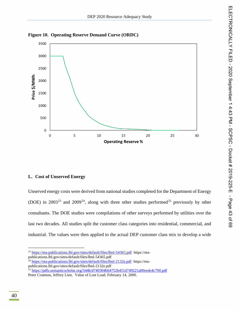
The cost of transfers between regions is based on marginal costs. In cases where a region is short
of resources, scarcity pricing is added to the marginal costs. As a region’s hourly reserves approach
zero, the scarcity pricing for that region increases. Figure 10 shows the scarcity pricing curve that
was used in the simulations. It should be noted that the frequency of these scarcity prices is very
low because in the majority of hours, there is plenty of capacity to meet load after the market has
cleared22.
22The market clearing algorithm within SERVM attempts to get all regions to the same price subject to transmission constraints. So, if a region’s original price is $3,000/MWh based on the conditions and scarcity pricing in that region alone, it is highly probable that a surrounding region will provide enough capacity to that region to bring prices down to reasonable levels.
ELECTR
ONICALLY
FILED-2020
September1
4:43PM
-SCPSC
-Docket#
2019-225-E-Page
42of69
DEP 2020 Resource Adequacy Study
40
Figure 10. Operating Reserve Demand Curve (ORDC)
L. Cost of Unserved Energy
Unserved energy costs were derived from national studies completed for the Department of Energy
(DOE) in 200323 and 200924, along with three other studies performed25 previously by other
consultants. The DOE studies were compilations of other surveys performed by utilities over the
last two decades. All studies split the customer class categories into residential, commercial, and
industrial. The values were then applied to the actual DEP customer class mix to develop a wide
23 https://eta-publications.lbl.gov/sites/default/files/lbnl-54365.pdf https://eta-publications.lbl.gov/sites/default/files/lbnl-54365.pdf 24 https://eta-publications.lbl.gov/sites/default/files/lbnl-2132e.pdf https://eta-publications.lbl.gov/sites/default/files/lbnl-2132e.pdf 25 https://pdfs.semanticscholar.org/544b/d740304b64752b451d749221a00eede4c700.pdf Peter Cramton, Jeffrey Lien. Value of Lost Load. February 14, 2000.
ELECTR
ONICALLY
FILED-2020
September1
4:43PM
-SCPSC
-Docket#
2019-225-E-Page
43of69
3500
3000
2500
& 2000
IJ 1500
1000
500
0
0 10 15
Operating Reserve%20 25 30

DEP 2020 Resource Adequacy Study
41
range of costs for unserved energy. Table 9 shows those results. Because expected unserved
energy costs are so low near the economic optimum reserve margin, this value, while high in
magnitude, is not a significant driver in the economic analysis. Since the public estimates ranged
significantly, DEP used $16,450/MWh for the Base Case in 2024, and sensitivities were performed
around this value from $5,000 MWh to $25,000 MWh to understand the impact.
Table 9. Unserved Energy Costs / Value of Lost Load
M. System Capacity Carrying Costs
The study assumes that the cheapest marginal resource is utilized to calculate the carrying cost of
additional capacity. The cost of carrying incremental reserves was based on the capital and FOM
of a new simple cycle natural gas Combustion Turbine (CT) consistent with the Company’s IRP
assumptions. For the study, the cost of each additional kW of reserves can be found in Confidential
Appendix Table CA6. The additional CT units were forced to have a 5% EFOR in the simulations
and used to vary reserve margin in the study.
ELECTR
ONICALLY
FILED-2020
September1
4:43PM
-SCPSC
-Docket#
2019-225-E-Page
44of69
W' s
2003 DOE Study
2024 5lcWh2009 DOE Study Chnstiansea Assomates Bilgnton and Wacker Karugu aad Agaa
2024 S'kWh 2024 SdcWh 2024 SlcWh 2024 SlcWh
Residenual
Commercial
ladustrial
43%33%24%
1 57
35 54
20 51
1.50
109.23
32.53
3.1222.3711.59
2.7323 2423.24
1 26
24 74
58 65
Weighted Average 5'kWh 17.31 44 55 11 50 14 38 22 60
Average S'kWhAverage S kV 'h exduding
the 2009 DOE Study
22 07
16 45
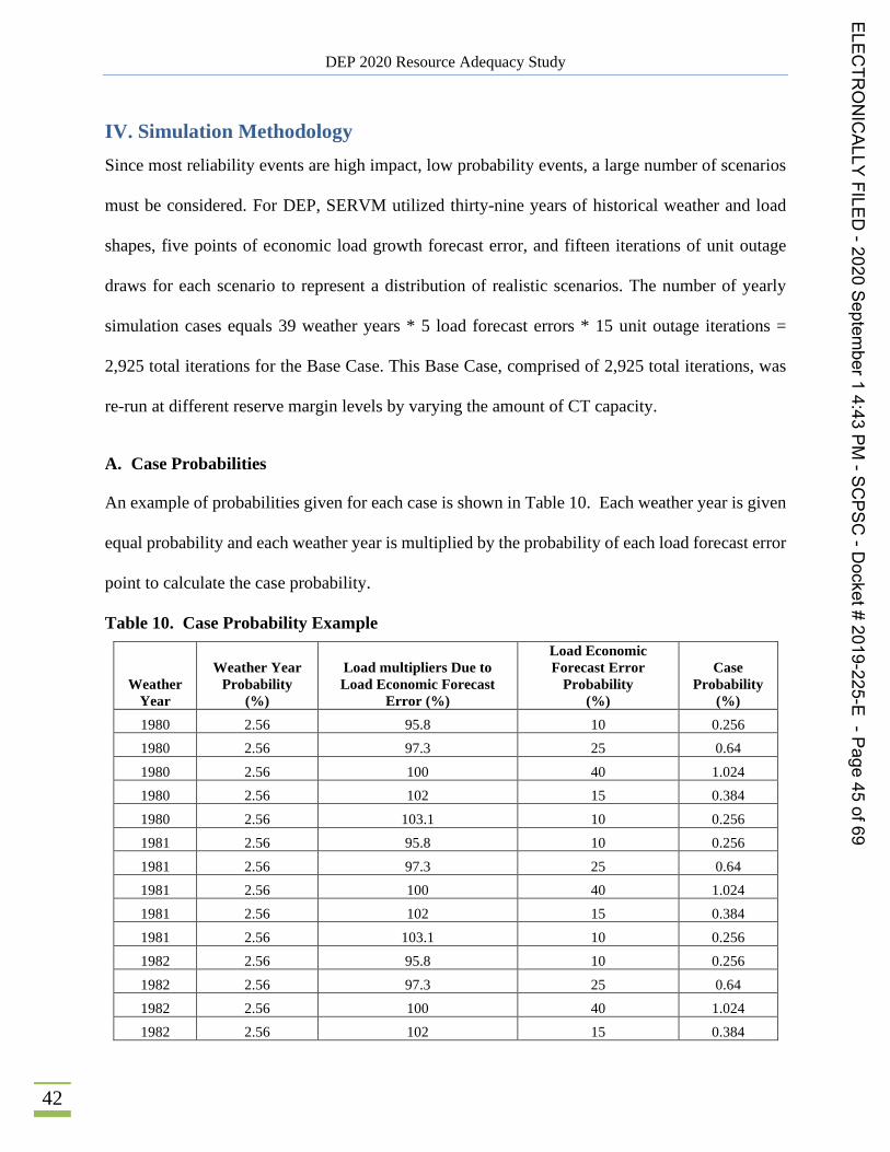
DEP 2020 Resource Adequacy Study
42
IV. Simulation Methodology Since most reliability events are high impact, low probability events, a large number of scenarios
must be considered. For DEP, SERVM utilized thirty-nine years of historical weather and load
shapes, five points of economic load growth forecast error, and fifteen iterations of unit outage
draws for each scenario to represent a distribution of realistic scenarios. The number of yearly
simulation cases equals 39 weather years * 5 load forecast errors * 15 unit outage iterations =
2,925 total iterations for the Base Case. This Base Case, comprised of 2,925 total iterations, was
re-run at different reserve margin levels by varying the amount of CT capacity.
A. Case Probabilities
An example of probabilities given for each case is shown in Table 10. Each weather year is given
equal probability and each weather year is multiplied by the probability of each load forecast error
point to calculate the case probability.
Table 10. Case Probability Example
Weather Year
Weather Year Probability
(%)
Load multipliers Due to Load Economic Forecast
Error (%)
Load Economic Forecast Error
Probability (%)
Case Probability
(%) 1980 2.56 95.8 10 0.256 1980 2.56 97.3 25 0.64 1980 2.56 100 40 1.024 1980 2.56 102 15 0.384 1980 2.56 103.1 10 0.256 1981 2.56 95.8 10 0.256 1981 2.56 97.3 25 0.64 1981 2.56 100 40 1.024 1981 2.56 102 15 0.384 1981 2.56 103.1 10 0.256 1982 2.56 95.8 10 0.256 1982 2.56 97.3 25 0.64 1982 2.56 100 40 1.024 1982 2.56 102 15 0.384
ELECTR
ONICALLY
FILED-2020
September1
4:43PM
-SCPSC
-Docket#
2019-225-E-Page
45of69

DEP 2020 Resource Adequacy Study
43
1982 2.56 103.1 10 0.256 ... ... ... ... ... ... ... ... ... ...
2018 2.56 103.1 10 0.256
Total 100
For this study, LOLE is defined in number of days per year and is calculated for each of the 195
load cases and weighted based on probability. When counting LOLE events, only one event is
counted per day even if an event occurs early in the day and then again later in the day. Across
the industry, the traditional 1 day in 10 year LOLE standard is defined as 0.1 LOLE. Additional
reliability metrics calculated are Loss of Load Hours (LOLH) in hours per year and Expected
Unserved Energy (EUE) in MWh.
Total system energy costs are defined as the following for each region: 𝑃𝑃𝑃𝑃𝑃𝑃𝑃𝑃𝑃𝑃𝑃𝑃𝑃𝑃𝑃𝑃𝑃𝑃𝑃𝑃 𝐶𝐶𝑃𝑃𝐶𝐶𝑃𝑃𝐶𝐶 (𝐹𝐹𝑃𝑃𝐹𝐹𝐹𝐹 𝐵𝐵𝑃𝑃𝑃𝑃𝑃𝑃 + 𝑉𝑉𝑉𝑉𝑃𝑃𝑃𝑃𝑉𝑉𝑉𝑉𝐹𝐹𝐹𝐹 𝑂𝑂&𝑀𝑀) + 𝑃𝑃𝑃𝑃𝑃𝑃𝑃𝑃ℎ𝑉𝑉𝐶𝐶𝐹𝐹 𝐶𝐶𝑃𝑃𝐶𝐶𝑃𝑃𝐶𝐶 − 𝑆𝑆𝑉𝑉𝐹𝐹𝐹𝐹𝐶𝐶 𝑅𝑅𝐹𝐹𝑅𝑅𝐹𝐹𝑃𝑃𝑃𝑃𝐹𝐹
+ 𝐿𝐿𝑃𝑃𝐶𝐶𝐶𝐶 𝑃𝑃𝑜𝑜 𝑅𝑅𝐹𝐹𝐶𝐶𝐹𝐹𝑃𝑃𝑅𝑅𝐹𝐹𝐶𝐶 + 𝐶𝐶𝑃𝑃𝐶𝐶𝑃𝑃 𝑃𝑃𝑜𝑜 𝑈𝑈𝑃𝑃𝐶𝐶𝐹𝐹𝑃𝑃𝑅𝑅𝐹𝐹𝑃𝑃 𝐸𝐸𝑃𝑃𝐹𝐹𝑃𝑃𝐸𝐸𝐸𝐸
These components are calculated for each case and weighted based on probability to calculate total
system energy costs for each scenario simulated. Loss of Reserves costs recognize the additional
risk of depleting operating reserves and are costed out at the ORDC curve when they occur. As
shown in the results these costs are almost negligible. The cost of unserved energy is simply the
MWh of load shed multiplied by the value of lost load. System capacity costs are calculated
separately outside of the SERVM model using the economic carrying cost of a new CT.
ELECTR
ONICALLY
FILED-2020
September1
4:43PM
-SCPSC
-Docket#
2019-225-E-Page
46of69
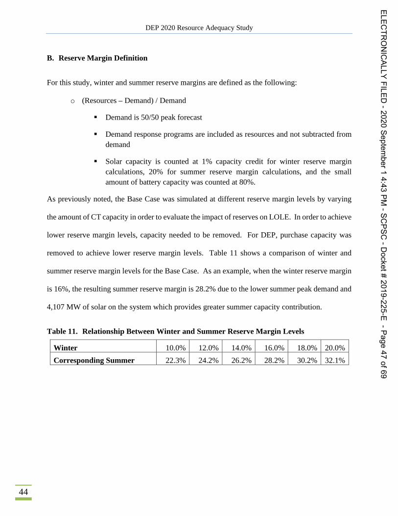
DEP 2020 Resource Adequacy Study
44
B. Reserve Margin Definition
For this study, winter and summer reserve margins are defined as the following:
o (Resources – Demand) / Demand
Demand is 50/50 peak forecast
Demand response programs are included as resources and not subtracted from demand
Solar capacity is counted at 1% capacity credit for winter reserve margin calculations, 20% for summer reserve margin calculations, and the small amount of battery capacity was counted at 80%.
As previously noted, the Base Case was simulated at different reserve margin levels by varying
the amount of CT capacity in order to evaluate the impact of reserves on LOLE. In order to achieve
lower reserve margin levels, capacity needed to be removed. For DEP, purchase capacity was
removed to achieve lower reserve margin levels. Table 11 shows a comparison of winter and
summer reserve margin levels for the Base Case. As an example, when the winter reserve margin
is 16%, the resulting summer reserve margin is 28.2% due to the lower summer peak demand and
4,107 MW of solar on the system which provides greater summer capacity contribution.
Table 11. Relationship Between Winter and Summer Reserve Margin Levels
Winter 10.0% 12.0% 14.0% 16.0% 18.0% 20.0% Corresponding Summer 22.3% 24.2% 26.2% 28.2% 30.2% 32.1%
ELECTR
ONICALLY
FILED-2020
September1
4:43PM
-SCPSC
-Docket#
2019-225-E-Page
47of69

DEP 2020 Resource Adequacy Study
45
V. Physical Reliability Results
Table 12 shows LOLE by month across a range of reserve margin levels for the Island Case. The
analysis shows all of the LOLE falls in the winter. To achieve reliability equivalent to the 1 day
in 10 year standard (0.1 LOLE) in the Island scenario, a 25.5% winter reserve margin is required.
Given the significant solar on the system, the summer reserves are approximately 12% greater than
winter reserves which results in no reliability risk in the summer months. This 25.5% reserve
margin is required to cover the combined risks seen in load uncertainty, weather uncertainty, and
generator performance for the DEP system.
Table 12. Island Physical Reliability Results
Winter Reserve Margin
Summer Reserve Margin
Jan Feb Mar Apr May Jun Jul Aug Sep Oct Nov Dec Summer LOLE
Winter LOLE
Total LOLE
10.0% 22.3% 0.43
0.09
0.06
0.00
0.00
0.00
0.00
0.00
0.00
0.00
0.00
0.12 0.00 0.70 0.71
11.0% 23.2% 0.37
0.08
0.05
0.00
0.00
0.00
0.00
0.00
0.00
0.00
0.00
0.11 0.00 0.61 0.62
12.0% 24.2% 0.32
0.07
0.04
0.00
0.00
0.00
0.00
0.00
0.00
0.00
0.00
0.10 0.00 0.53 0.54
13.0% 25.2% 0.28
0.06
0.04
0.00
0.00
0.00
0.00
0.00
0.00
0.00
0.00
0.08 0.00 0.47 0.47
14.0% 26.2% 0.25
0.06
0.03
0.00
0.00
0.00
0.00
0.00
0.00
0.00
0.00
0.07 0.00 0.41 0.41
15.0% 27.2% 0.21
0.06
0.03
0.00
0.00
0.00
0.00
0.00
0.00
0.00
0.00
0.06 0.00 0.35 0.36
16.0% 28.2% 0.19
0.05
0.03
0.00
0.00
0.00
0.00
0.00
0.00
0.00
0.00
0.05 0.00 0.31 0.31
17.0% 29.1% 0.17
0.05
0.02
0.00
0.00
0.00
0.00
0.00
0.00
0.00
0.00
0.04 0.00 0.28 0.28
18.0% 30.1% 0.15
0.05
0.02
0.00
0.00
0.00
0.00
0.00
0.00
0.00
0.00
0.03 0.00 0.25 0.25
19.0% 31.1% 0.13
0.04
0.02
0.00
0.00
0.00
0.00
0.00
0.00
0.00
0.00
0.03 0.00 0.22 0.22
20.0% 32.1% 0.12
0.04
0.01
0.00
0.00
0.00
0.00
0.00
0.00
0.00
0.00
0.03 0.00 0.20 0.20
21.0% 33.1% 0.11
0.04
0.01
0.00
0.00
0.00
0.00
0.00
0.00
0.00
0.00
0.03 0.00 0.18 0.18
22.0% 34.1% 0.10
0.04
0.00
0.00
0.00
0.00
0.00
0.00
0.00
0.00
0.00
0.02 0.00 0.16 0.16
23.0% 35.1% 0.09
0.03
0.00
0.00
0.00
0.00
0.00
0.00
0.00
0.00
0.00
0.02 0.00 0.14 0.14
24.0% 36.0% 0.08
0.03
0.01
0.00
0.00
0.00
0.00
0.00
0.00
0.00
0.00
0.01 0.00 0.12 0.12
25.0% 37.0% 0.07
0.03
0.00
0.00
0.00
0.00
0.00
0.00
0.00
0.00
0.00
0.01 0.00 0.11 0.11
26.0% 38.0% 0.06
0.02
0.00
0.00
0.00
0.00
0.00
0.00
0.00
0.00
0.00
0.02 0.00 0.10 0.10
ELECTR
ONICALLY
FILED-2020
September1
4:43PM
-SCPSC
-Docket#
2019-225-E-Page
48of69
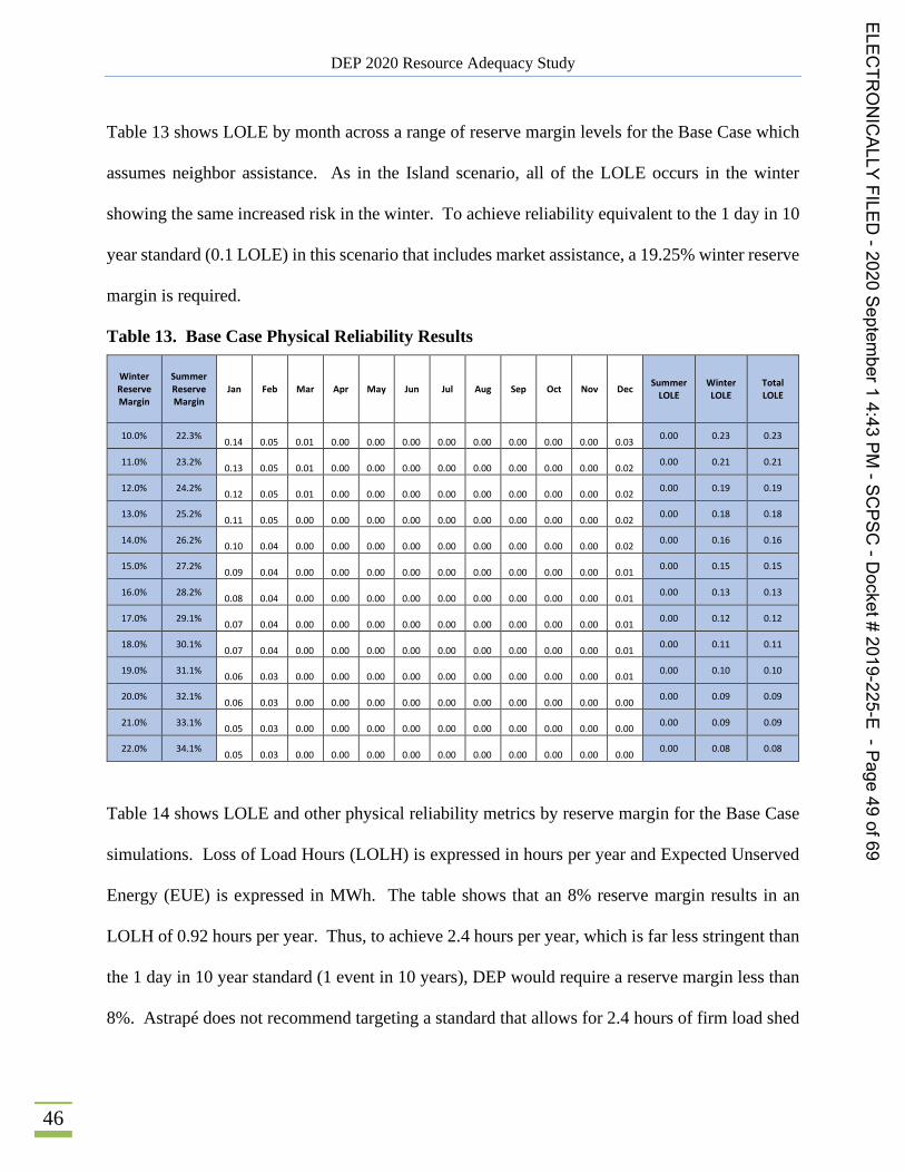
DEP 2020 Resource Adequacy Study
46
Table 13 shows LOLE by month across a range of reserve margin levels for the Base Case which
assumes neighbor assistance. As in the Island scenario, all of the LOLE occurs in the winter
showing the same increased risk in the winter. To achieve reliability equivalent to the 1 day in 10
year standard (0.1 LOLE) in this scenario that includes market assistance, a 19.25% winter reserve
margin is required.
Table 13. Base Case Physical Reliability Results
Winter Reserve Margin
Summer Reserve Margin
Jan Feb Mar Apr May Jun Jul Aug Sep Oct Nov Dec Summer LOLE
Winter LOLE
Total LOLE
10.0% 22.3% 0.14
0.05
0.01
0.00
0.00
0.00
0.00
0.00
0.00
0.00
0.00
0.03 0.00 0.23 0.23
11.0% 23.2% 0.13
0.05
0.01
0.00
0.00
0.00
0.00
0.00
0.00
0.00
0.00
0.02 0.00 0.21 0.21
12.0% 24.2% 0.12
0.05
0.01
0.00
0.00
0.00
0.00
0.00
0.00
0.00
0.00
0.02 0.00 0.19 0.19
13.0% 25.2% 0.11
0.05
0.00
0.00
0.00
0.00
0.00
0.00
0.00
0.00
0.00
0.02 0.00 0.18 0.18
14.0% 26.2% 0.10
0.04
0.00
0.00
0.00
0.00
0.00
0.00
0.00
0.00
0.00
0.02 0.00 0.16 0.16
15.0% 27.2% 0.09
0.04
0.00
0.00
0.00
0.00
0.00
0.00
0.00
0.00
0.00
0.01 0.00 0.15 0.15
16.0% 28.2% 0.08
0.04
0.00
0.00
0.00
0.00
0.00
0.00
0.00
0.00
0.00
0.01 0.00 0.13 0.13
17.0% 29.1% 0.07
0.04
0.00
0.00
0.00
0.00
0.00
0.00
0.00
0.00
0.00
0.01 0.00 0.12 0.12
18.0% 30.1% 0.07
0.04
0.00
0.00
0.00
0.00
0.00
0.00
0.00
0.00
0.00
0.01 0.00 0.11 0.11
19.0% 31.1% 0.06
0.03
0.00
0.00
0.00
0.00
0.00
0.00
0.00
0.00
0.00
0.01 0.00 0.10 0.10
20.0% 32.1% 0.06
0.03
0.00
0.00
0.00
0.00
0.00
0.00
0.00
0.00
0.00
0.00 0.00 0.09 0.09
21.0% 33.1% 0.05
0.03
0.00
0.00
0.00
0.00
0.00
0.00
0.00
0.00
0.00
0.00 0.00 0.09 0.09
22.0% 34.1% 0.05
0.03
0.00
0.00
0.00
0.00
0.00
0.00
0.00
0.00
0.00
0.00 0.00 0.08 0.08
Table 14 shows LOLE and other physical reliability metrics by reserve margin for the Base Case
simulations. Loss of Load Hours (LOLH) is expressed in hours per year and Expected Unserved
Energy (EUE) is expressed in MWh. The table shows that an 8% reserve margin results in an
LOLH of 0.92 hours per year. Thus, to achieve 2.4 hours per year, which is far less stringent than
the 1 day in 10 year standard (1 event in 10 years), DEP would require a reserve margin less than
8%. Astrapé does not recommend targeting a standard that allows for 2.4 hours of firm load shed
ELECTR
ONICALLY
FILED-2020
September1
4:43PM
-SCPSC
-Docket#
2019-225-E-Page
49of69
DEP 2020 Resource Adequacy Study
47
every year as essentially would expect a firm load shed during peak periods ever year. The hours
per event can be calculated by dividing LOLH by LOLE. The firm load shed events last
approximately 2-3 hours on average. As these reserve margins decrease and firm load shed events
increase, it is expected that reliance on external assistance, depletion of contingency reserves, and
more demand response calls will occur and increase the overall reliability risk on the system.
ELECTR
ONICALLY
FILED-2020
September1
4:43PM
-SCPSC
-Docket#
2019-225-E-Page
50of69
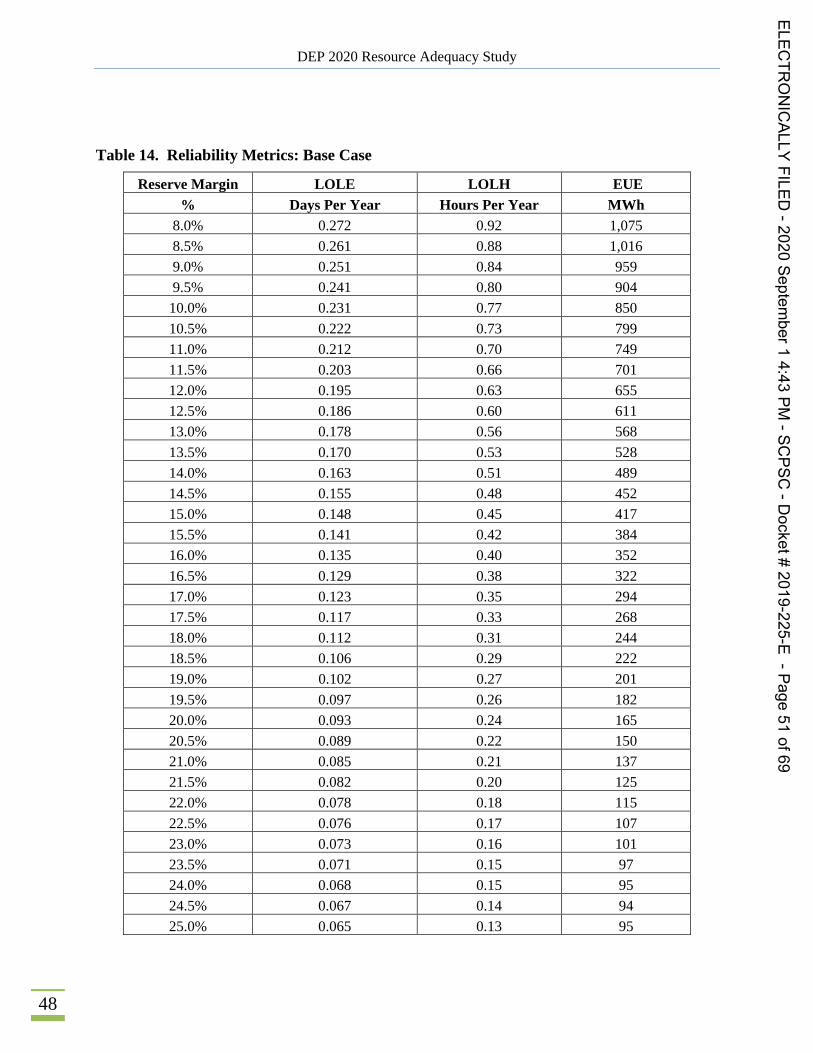
DEP 2020 Resource Adequacy Study
48
Table 14. Reliability Metrics: Base Case
Reserve Margin LOLE LOLH EUE % Days Per Year Hours Per Year MWh
8.0% 0.272 0.92 1,075 8.5% 0.261 0.88 1,016 9.0% 0.251 0.84 959 9.5% 0.241 0.80 904 10.0% 0.231 0.77 850 10.5% 0.222 0.73 799 11.0% 0.212 0.70 749 11.5% 0.203 0.66 701 12.0% 0.195 0.63 655 12.5% 0.186 0.60 611 13.0% 0.178 0.56 568 13.5% 0.170 0.53 528 14.0% 0.163 0.51 489 14.5% 0.155 0.48 452 15.0% 0.148 0.45 417 15.5% 0.141 0.42 384 16.0% 0.135 0.40 352 16.5% 0.129 0.38 322 17.0% 0.123 0.35 294 17.5% 0.117 0.33 268 18.0% 0.112 0.31 244 18.5% 0.106 0.29 222 19.0% 0.102 0.27 201 19.5% 0.097 0.26 182 20.0% 0.093 0.24 165 20.5% 0.089 0.22 150 21.0% 0.085 0.21 137 21.5% 0.082 0.20 125 22.0% 0.078 0.18 115 22.5% 0.076 0.17 107 23.0% 0.073 0.16 101 23.5% 0.071 0.15 97 24.0% 0.068 0.15 95 24.5% 0.067 0.14 94 25.0% 0.065 0.13 95
ELECTR
ONICALLY
FILED-2020
September1
4:43PM
-SCPSC
-Docket#
2019-225-E-Page
51of69

DEP 2020 Resource Adequacy Study
49
VI. Base Case Economic Results
While Astrapé believes physical reliability metrics should be used for determining planning
reserve margin because customers expect to have power during extreme weather conditions,
customer costs provide additional information in resource adequacy studies. From a customer cost
perspective, total system costs were analyzed across reserve margin levels for the Base Case.
Figure 11 shows the risk neutral costs at the various winter reserve margin levels. This risk neutral
represents the weighted average results of all weather years, load forecast uncertainty, and unit
performance iterations at each reserve margin level and represents the expected value on a year in
and year out basis.
Figure 11. Base Case Risk Neutral Economic Results26
26 Costs that are included in every reserve margin level have been removed so the reader can see the incremental impact of each category of costs. DEP has approximately 1 billion dollars in total costs.
ELECTR
ONICALLY
FILED-2020
September1
4:43PM
-SCPSC
-Docket#
2019-225-E-Page
52of69
160,000,0M
140,000,000
120,000,000
100,000,000
0 60,000,000
o60,000,0M
40,000,000
20,000,0M
5% 6% 7% 6% 9% 10% 11'%26 13% 14% 15% 16% 12% 16% 19!6 20% 21% 22%
Winter Reserve Margin
~ CT Costs ~ Pro Casts ~ Net Purchases ~ Loss of Reserves ~ EUE Costs

DEP 2020 Resource Adequacy Study
50
As Figure 11 shows, the lowest risk neutral cost falls at a 10.25% reserve margin. The reason this
risk neutral reserve margin is significantly lower than 19.25% reserve margin required to meet the
0.1 LOLE is due to high reserve margins in the summer. The majority of the savings seen in
adding additional capacity is recognized in the winter.27 The cost curve is fairly flat for a large
portion of the reserve margin curve because when CT capacity is added there is always system
energy cost savings from either reduction in loss of load events, savings in purchases, or savings
in production costs. This risk neutral scenario represents the weighted average of all scenarios but
does not illustrate the impact of high-risk scenarios that could cause customer rates to be volatile
from year to year. Figure 12, however, shows the distribution of system energy costs (production
costs, purchase costs, loss of reserves costs, and the costs of EUE) at different reserve margin
levels. This figure excludes fixed CT costs which increase with reserve margin level. As reserves
are added, system energy costs decline. By moving from lower reserve margins to higher reserve
margins, the volatile right side of the curve (greater than 85% Cumulative Probability) is
dampened, shielding customers from extreme scenarios for relatively small increases in annual
expected costs. By paying for additional CT capacity, extreme scenarios are mitigated.
27 As the DEC study shows, the lower DEC summer reserve margins increase the risk neutral economic reserve margin level compared to the DEP Study.
ELECTR
ONICALLY
FILED-2020
September1
4:43PM
-SCPSC
-Docket#
2019-225-E-Page
53of69
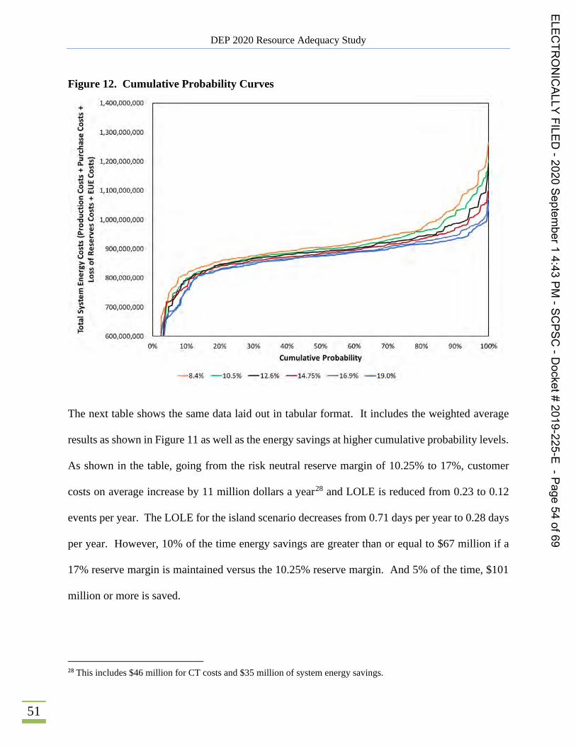
DEP 2020 Resource Adequacy Study
51
Figure 12. Cumulative Probability Curves
The next table shows the same data laid out in tabular format. It includes the weighted average
results as shown in Figure 11 as well as the energy savings at higher cumulative probability levels.
As shown in the table, going from the risk neutral reserve margin of 10.25% to 17%, customer
costs on average increase by 11 million dollars a year28 and LOLE is reduced from 0.23 to 0.12
events per year. The LOLE for the island scenario decreases from 0.71 days per year to 0.28 days
per year. However, 10% of the time energy savings are greater than or equal to $67 million if a
17% reserve margin is maintained versus the 10.25% reserve margin. And 5% of the time, $101
million or more is saved.
28 This includes $46 million for CT costs and $35 million of system energy savings.
ELECTR
ONICALLY
FILED-2020
September1
4:43PM
-SCPSC
-Docket#
2019-225-E-Page
54of69
+N
0VUl
UI
I/
UL
+N V
UI0IJ IUC
~80V00. U
IU0 ICV0
UI0 0IU
EUl
I/I
Ul
0
1,400,000,000
1,300,000,000
1,200,000,000
1,100,000,000
1,000,000,000
900,000,000
800,000,000
700,000,000
600,000,0000% 10% 20% 30% 40% 50% 60% 70'%0% 90% 100%
Cumulative Probability
8.4% —106% 12.6% —14.75% —16.9% 19.0%
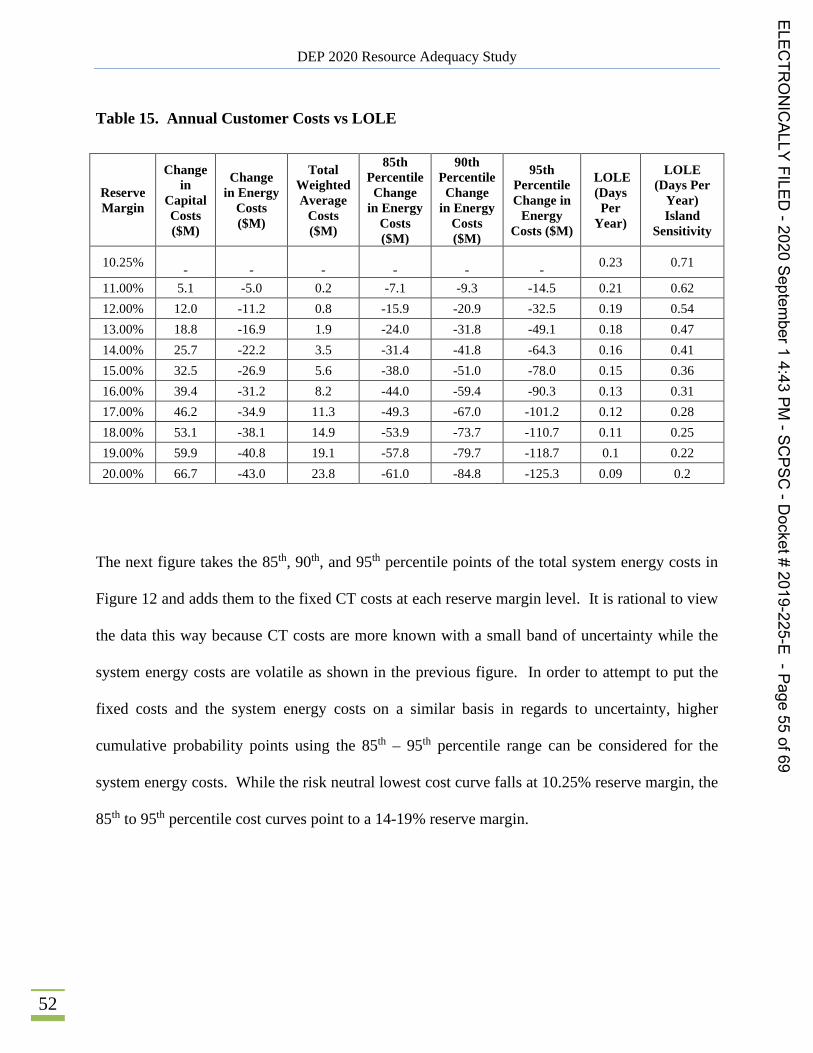
DEP 2020 Resource Adequacy Study
52
Table 15. Annual Customer Costs vs LOLE
Reserve Margin
Change in
Capital Costs ($M)
Change in Energy
Costs ($M)
Total Weighted Average
Costs ($M)
85th Percentile Change
in Energy Costs ($M)
90th Percentile
Change in Energy
Costs ($M)
95th Percentile Change in
Energy Costs ($M)
LOLE (Days Per
Year)
LOLE (Days Per
Year) Island
Sensitivity
10.25% -
-
-
-
-
- 0.23 0.71
11.00% 5.1 -5.0 0.2 -7.1 -9.3 -14.5 0.21 0.62 12.00% 12.0 -11.2 0.8 -15.9 -20.9 -32.5 0.19 0.54 13.00% 18.8 -16.9 1.9 -24.0 -31.8 -49.1 0.18 0.47 14.00% 25.7 -22.2 3.5 -31.4 -41.8 -64.3 0.16 0.41 15.00% 32.5 -26.9 5.6 -38.0 -51.0 -78.0 0.15 0.36 16.00% 39.4 -31.2 8.2 -44.0 -59.4 -90.3 0.13 0.31 17.00% 46.2 -34.9 11.3 -49.3 -67.0 -101.2 0.12 0.28 18.00% 53.1 -38.1 14.9 -53.9 -73.7 -110.7 0.11 0.25 19.00% 59.9 -40.8 19.1 -57.8 -79.7 -118.7 0.1 0.22 20.00% 66.7 -43.0 23.8 -61.0 -84.8 -125.3 0.09 0.2
The next figure takes the 85th, 90th, and 95th percentile points of the total system energy costs in
Figure 12 and adds them to the fixed CT costs at each reserve margin level. It is rational to view
the data this way because CT costs are more known with a small band of uncertainty while the
system energy costs are volatile as shown in the previous figure. In order to attempt to put the
fixed costs and the system energy costs on a similar basis in regards to uncertainty, higher
cumulative probability points using the 85th – 95th percentile range can be considered for the
system energy costs. While the risk neutral lowest cost curve falls at 10.25% reserve margin, the
85th to 95th percentile cost curves point to a 14-19% reserve margin.
ELECTR
ONICALLY
FILED-2020
September1
4:43PM
-SCPSC
-Docket#
2019-225-E-Page
55of69
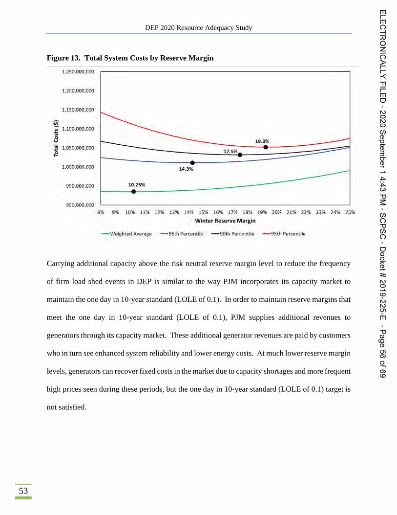
DEP 2020 Resource Adequacy Study
53
Figure 13. Total System Costs by Reserve Margin
Carrying additional capacity above the risk neutral reserve margin level to reduce the frequency
of firm load shed events in DEP is similar to the way PJM incorporates its capacity market to
maintain the one day in 10-year standard (LOLE of 0.1). In order to maintain reserve margins that
meet the one day in 10-year standard (LOLE of 0.1), PJM supplies additional revenues to
generators through its capacity market. These additional generator revenues are paid by customers
who in turn see enhanced system reliability and lower energy costs. At much lower reserve margin
levels, generators can recover fixed costs in the market due to capacity shortages and more frequent
high prices seen during these periods, but the one day in 10-year standard (LOLE of 0.1) target is
not satisfied.
ELECTR
ONICALLY
FILED-2020
September1
4:43PM
-SCPSC
-Docket#
2019-225-E-Page
56of69
1,250,000,00D
1,200,000,000
1, 150,000,000
vi 1,100,000,000Ih0Vni 1,050,000,000
HO
1,000,000,DOO
950,000,000
900,000,0008% 9'%0% 11% 12% 13% 14% 15% 16% 17% 18% 19% 20% 21% 22% 23% 24% 25%
Winter Reserve Margin
—Weighted Average —85th Percentile —90th Percentile —95th Percentile

DEP 2020 Resource Adequacy Study
54
VII. Sensitivities
Several sensitivities were simulated in order to understand the effects of different assumptions on
the 0.1 LOLE minimum winter reserve margin and to address questions and requests from
stakeholders.
Outage Sensitivities
As previously noted, the Base Case included a total of 400 MW of cold weather outages between
DEC and DEP below ten degrees Fahrenheit based on outage data for the period 2016-2019.
Sensitivities were run to see the effect of two cold weather outage assumptions. The first assumed
that the 400 MW of total outages between DEC and DEP below ten degrees Fahrenheit were
removed. As Table 16 indicates, the minimum reserve margin for the one day in 10-year standard
(LOLE of 0.1) is lowered by 0.75% from the Base Case to 18.50%. This shows that if the Company
was able to eliminate all cold weather outage risk, it could carry up to a 0.75% lower reserve
margin. However, Astrapé recognizes based on North American Electric Reliability Corporation
(NERC) documentation across the industry29 that outages during cold temperatures could be
substantially more than the 400 MW being applied at less than 10 degrees in this modeling.
29 https://www.nerc.com/pa/RAPA/ra/Reliability%20Assessments%20DL/NERC%20WRA%202019_2020.pdfvv(page 5)
https://www.nerc.com/pa/rrm/ea/Documents/South_Central_Cold_Weather_Event_FERC-NERC-Report_20190718.pdf
(beginning page 43)
ELECTR
ONICALLY
FILED-2020
September1
4:43PM
-SCPSC
-Docket#
2019-225-E-Page
57of69

DEP 2020 Resource Adequacy Study
55
Table 16. No Cold Weather Outage Results
LOLE Economics
Sensitivity 1 in 10 Weighted
Average (risk neutral)
90th %
Base Case 19.25% 10.25% 17.50% No Cold Weather
Outages 18.50% 9.50% 16.25%
The second outage sensitivity showed what the minimum reserve margin for the one day in 10-
year standard (LOLE of 0.1) would need to be if cold weather outages were based solely on 2014-
2019 historical data which increased the total MW of outages from 400 MW to 800 MW. Table
17 shows that the minimum reserve margin for 0.1 LOLE is 20.50 %.
Table 17. Cold Weather Outages Based on 2014-2019 Results
LOLE Economics
Sensitivity 1 in 10 Weighted
Average (risk neutral)
90th %
Base Case 19.25% 10.25% 17.50% Cold Weather
Outages Based on 2014 - 2019
20.50% 10.50% 17.75%
Load Forecast Error Sensitivities
These sensitivities were run to see the effects of the Load Forecast Error (LFE) assumptions. In
response to stakeholder feedback, an asymmetric LFE distribution was adopted in the Base Case
which reflected a higher probability weighting on over-forecasting scenarios. In the first
sensitivity, the LFE uncertainty was completely removed. The minimum reserve margin for the
one day in 10-year standard (LOLE of 0.1) increased by 0.75% to 20.00%. This demonstrates that
the load forecast error assumed in the Base Case was reducing the target reserve margin levels
ELECTR
ONICALLY
FILED-2020
September1
4:43PM
-SCPSC
-Docket#
2019-225-E-Page
58of69
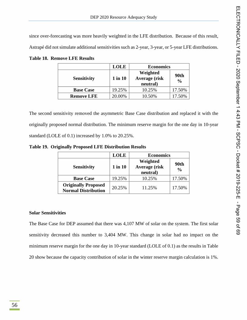
DEP 2020 Resource Adequacy Study
56
since over-forecasting was more heavily weighted in the LFE distribution. Because of this result,
Astrapé did not simulate additional sensitivities such as 2-year, 3-year, or 5-year LFE distributions.
Table 18. Remove LFE Results
LOLE Economics
Sensitivity 1 in 10 Weighted
Average (risk neutral)
90th %
Base Case 19.25% 10.25% 17.50% Remove LFE 20.00% 10.50% 17.50%
The second sensitivity removed the asymmetric Base Case distribution and replaced it with the
originally proposed normal distribution. The minimum reserve margin for the one day in 10-year
standard (LOLE of 0.1) increased by 1.0% to 20.25%.
Table 19. Originally Proposed LFE Distribution Results
LOLE Economics
Sensitivity 1 in 10 Weighted
Average (risk neutral)
90th %
Base Case 19.25% 10.25% 17.50% Originally Proposed Normal Distribution 20.25% 11.25% 17.50%
Solar Sensitivities
The Base Case for DEP assumed that there was 4,107 MW of solar on the system. The first solar
sensitivity decreased this number to 3,404 MW. This change in solar had no impact on the
minimum reserve margin for the one day in 10-year standard (LOLE of 0.1) as the results in Table
20 show because the capacity contribution of solar in the winter reserve margin calculation is 1%.
ELECTR
ONICALLY
FILED-2020
September1
4:43PM
-SCPSC
-Docket#
2019-225-E-Page
59of69
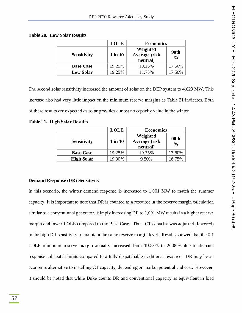
DEP 2020 Resource Adequacy Study
57
Table 20. Low Solar Results
LOLE Economics
Sensitivity 1 in 10 Weighted
Average (risk neutral)
90th %
Base Case 19.25% 10.25% 17.50% Low Solar 19.25% 11.75% 17.50%
The second solar sensitivity increased the amount of solar on the DEP system to 4,629 MW. This
increase also had very little impact on the minimum reserve margins as Table 21 indicates. Both
of these results are expected as solar provides almost no capacity value in the winter.
Table 21. High Solar Results
LOLE Economics
Sensitivity 1 in 10 Weighted
Average (risk neutral)
90th %
Base Case 19.25% 10.25% 17.50% High Solar 19.00% 9.50% 16.75%
Demand Response (DR) Sensitivity
In this scenario, the winter demand response is increased to 1,001 MW to match the summer
capacity. It is important to note that DR is counted as a resource in the reserve margin calculation
similar to a conventional generator. Simply increasing DR to 1,001 MW results in a higher reserve
margin and lower LOLE compared to the Base Case. Thus, CT capacity was adjusted (lowered)
in the high DR sensitivity to maintain the same reserve margin level. Results showed that the 0.1
LOLE minimum reserve margin actually increased from 19.25% to 20.00% due to demand
response’s dispatch limits compared to a fully dispatchable traditional resource. DR may be an
economic alternative to installing CT capacity, depending on market potential and cost. However,
it should be noted that while Duke counts DR and conventional capacity as equivalent in load
ELECTR
ONICALLY
FILED-2020
September1
4:43PM
-SCPSC
-Docket#
2019-225-E-Page
60of69

DEP 2020 Resource Adequacy Study
58
carrying capability in its IRP planning, the sensitivity results show that DR may have a slightly
lower equivalent load carrying capability especially for programs with strict operational limits.
The results are listed in Table 22 below.
Table 22. Demand Response Results
LOLE Economics
Sensitivity 1 in 10 Weighted
Average (risk neutral)
90th %
Base Case 19.25% 10.25% 17.50% Demand Response Winter as High as
Summer 20.00% 12.50% 18.50%
No Coal Sensitivity
In this scenario, all coal units were replaced with CC/CT units. The CC units were modeled with
a 4% EFOR and the CT units were modeled with a 5% EFOR. Due to the low EFOR’s of the DEP
coal units, the minimum reserve margin for the one day in 10-year standard (LOLE of 0.1)
increased slightly as shown in Table 23 below. Essentially these thermal resources were
interchangeable and had a minimal impact on the reserve margin.
Table 23. No Coal Results
LOLE Economics
Sensitivity 1 in 10 Weighted
Average (risk neutral)
90th %
Base Case 19.25% 10.25% 17.50% Retire all Coal 19.50% 11.25% 17.50%
ELECTR
ONICALLY
FILED-2020
September1
4:43PM
-SCPSC
-Docket#
2019-225-E-Page
61of69
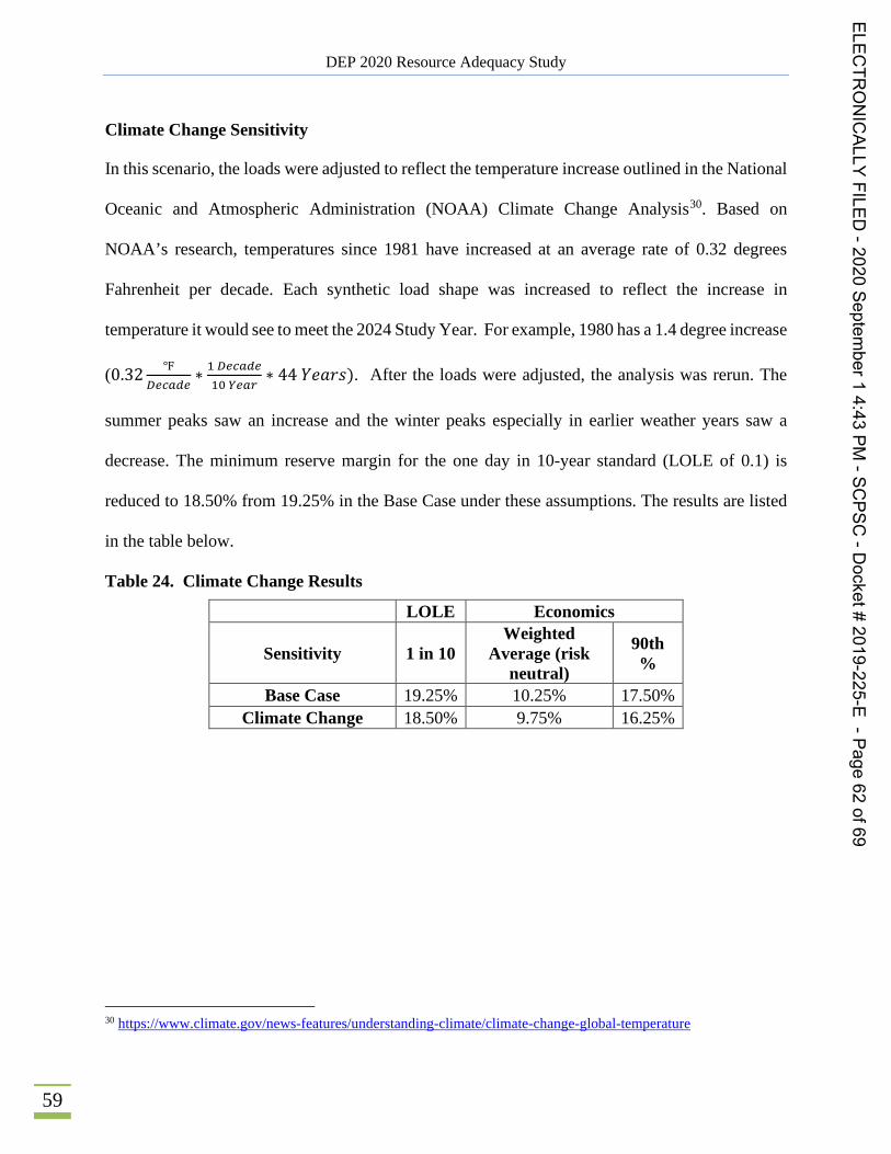
DEP 2020 Resource Adequacy Study
59
Climate Change Sensitivity
In this scenario, the loads were adjusted to reflect the temperature increase outlined in the National
Oceanic and Atmospheric Administration (NOAA) Climate Change Analysis30. Based on
NOAA’s research, temperatures since 1981 have increased at an average rate of 0.32 degrees
Fahrenheit per decade. Each synthetic load shape was increased to reflect the increase in
temperature it would see to meet the 2024 Study Year. For example, 1980 has a 1.4 degree increase
(0.32 ℉𝐷𝐷𝐷𝐷𝐷𝐷𝐷𝐷𝐷𝐷𝐷𝐷
∗ 1 𝐷𝐷𝐷𝐷𝐷𝐷𝐷𝐷𝐷𝐷𝐷𝐷10 𝑌𝑌𝐷𝐷𝐷𝐷𝑌𝑌
∗ 44 𝑌𝑌𝐹𝐹𝑉𝑉𝑃𝑃𝐶𝐶). After the loads were adjusted, the analysis was rerun. The
summer peaks saw an increase and the winter peaks especially in earlier weather years saw a
decrease. The minimum reserve margin for the one day in 10-year standard (LOLE of 0.1) is
reduced to 18.50% from 19.25% in the Base Case under these assumptions. The results are listed
in the table below.
Table 24. Climate Change Results
LOLE Economics
Sensitivity 1 in 10 Weighted
Average (risk neutral)
90th %
Base Case 19.25% 10.25% 17.50% Climate Change 18.50% 9.75% 16.25%
30 https://www.climate.gov/news-features/understanding-climate/climate-change-global-temperature
ELECTR
ONICALLY
FILED-2020
September1
4:43PM
-SCPSC
-Docket#
2019-225-E-Page
62of69
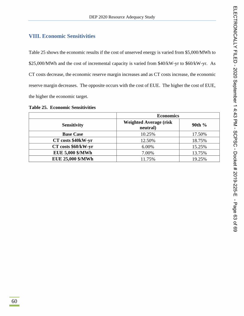
DEP 2020 Resource Adequacy Study
60
VIII. Economic Sensitivities
Table 25 shows the economic results if the cost of unserved energy is varied from $5,000/MWh to
$25,000/MWh and the cost of incremental capacity is varied from $40/kW-yr to $60/kW-yr. As
CT costs decrease, the economic reserve margin increases and as CT costs increase, the economic
reserve margin decreases. The opposite occurs with the cost of EUE. The higher the cost of EUE,
the higher the economic target.
Table 25. Economic Sensitivities
Economics
Sensitivity Weighted Average (risk neutral) 90th %
Base Case 10.25% 17.50% CT costs $40kW-yr 12.50% 18.75% CT costs $60/kW-yr 6.00% 15.25% EUE 5,000 $/MWh 7.00% 13.75% EUE 25,000 $/MWh 11.75% 19.25%
ELECTR
ONICALLY
FILED-2020
September1
4:43PM
-SCPSC
-Docket#
2019-225-E-Page
63of69

DEP 2020 Resource Adequacy Study
61
IX. DEC/DEP Combined Sensitivity
A set of sensitivities was performed which assumed DEC, DEP-E, and DEP-W were dispatched
together and all reserves were calculated as a single company across the three regions. In these
scenarios, all resources down to the firm load shed point can be utilized to assist each other and
there is a priority in assisting each other before assisting an outside neighbor. The following three
scenarios were simulated for the Combined Case and their results are listed in the table below:
1) Combined-Base
2) Combined Target 1,500 MW Import Limit - This scenario assumed a maximum import
limit from external regions into the sister utilities of 1,500 MW31.
3) Combined-Remove LFE
As shown in the table below, the combined target scenario yielded a 0.1 LOLE reserve margin of
16.75% (based on DEP and DEC coincident peak).
Table 26. Combined Case Results
LOLE Economics
Sensitivity 1 in 10 weighted avg (risk neutral) 90th %
Base Case 19.25% 10.25% 17.50% Combined Target 16.75% 17.00% 17.75%
Combined Target 1,500 MW Import Limit 18.00% 17.25% 18.25%
Combined Target - Remove LFE 17.25% 17.00% 18.25%
31 1,500 MW represents approximately 4.7% of the total reserve margin requirement which is still less constrained than the PJM and MISO assumptions noted earlier.
ELECTR
ONICALLY
FILED-2020
September1
4:43PM
-SCPSC
-Docket#
2019-225-E-Page
64of69
DEP 2020 Resource Adequacy Study
62
X. Conclusions
Based on the physical reliability results of the Island, Base Case, Combined Case, additional
sensitivities, as well as the results of the separate DEC Study, Astrapé recommends that DEP
continue to maintain a minimum 17% reserve margin for IRP purposes. This reserve margin
ensures reasonable reliability for customers. Astrapé recognizes that a standalone DEP utility
would require a 25.5% reserve margin to meet the one day in 10-year standard (LOLE of 0.1) and
even with market assistance, DEP would need to maintain a 19.25% reserve margin. Customers
expect electricity during extreme hot and cold weather conditions and maintaining a 17% reserve
margin is estimated to provide an LOLE of 0.12 events per year which is slightly less reliable than
the one day in 10-year standard (LOLE of 0.1). However, given the combined DEC and DEP
sensitivity resulting in a 16.75% reserve margin, and the 16% reserve margin required by DEC to
meet the one day in 10-year standard (LOLE of 0.1), Astrapé believes the 17% reserve margin as
a minimum target is still reasonable for planning purposes. Since the sensitivity results removing
all economic load forecast uncertainty increases the reserve margin to meet the 1 day in 10-year
standard, Astrapé believes this 17% minimum reserve margin should be used in the short- and
long-term planning process.
To be clear, even with 17% reserves, this does not mean that DEP will never be forced to shed
firm load during extreme conditions as DEP and its neighbors shift to reliance on intermittent and
energy limited resources such as storage and demand response. DEP has had several events in the
past few years where actual operating reserves were close to being exhausted even with higher
than 17% planning reserve margins. But if not for non-firm external assistance which this study
considers, firm load would have been shed. In addition, incorporation of tail end reliability risk in
ELECTR
ONICALLY
FILED-2020
September1
4:43PM
-SCPSC
-Docket#
2019-225-E-Page
65of69
DEP 2020 Resource Adequacy Study
63
modeling should be from statistically and historically defendable methods; not from including
subjective risks that cannot be assigned probability. Astrapé’s approach has been to model the
system’s risks around weather, load, generator performance, and market assistance as accurately
as possible without overly conservative assumptions. Based on all results, Astrapé believes
planning to a 17% reserve margin is prudent from a physical reliability perspective and for small
increases in costs above the risk-neutral 10.25% reserve margin level, customers will experience
enhanced reliability and less rate volatility.
As the DEP resource portfolio changes with the addition of more intermittent resources and energy
limited resources, the 17% minimum reserve margin is sufficient as long as the Company has
accounted for the capacity value of solar and battery resources which changes as a function of
penetration. DEP should also monitor changes in the IRPs of neighboring utilities and the potential
impact on market assistance. Unless DEP observes seasonal risk shifting back to summer, the
17% reserve margin should be reasonable but should be re-evaluated as appropriate in future IRPs
and future reliability studies. To ensure summer reliability is maintained, Astrapé recommends
not allowing the summer reserve margin to drop below 15%.32
32 Currently, if a winter target is maintained at 17%, summer reserves will be above 15%.
ELECTR
ONICALLY
FILED-2020
September1
4:43PM
-SCPSC
-Docket#
2019-225-E-Page
66of69
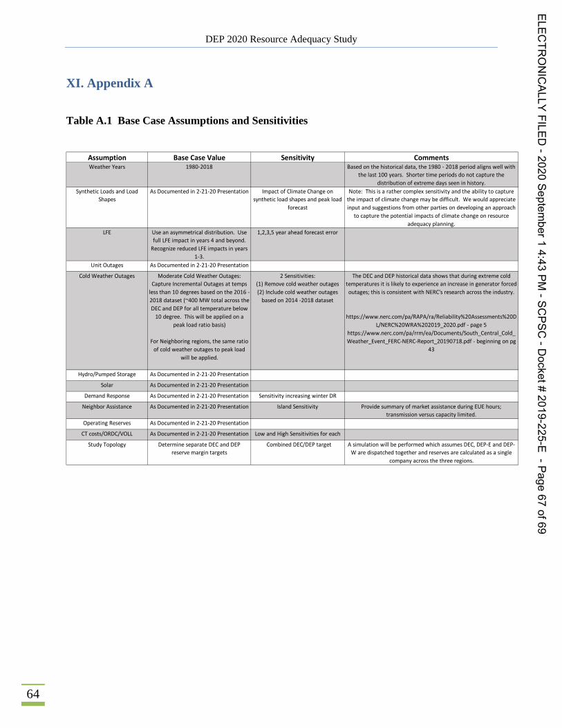
DEP 2020 Resource Adequacy Study
64
XI. Appendix A
Table A.1 Base Case Assumptions and Sensitivities
Assumption Base Case Value Sensitivity CommentsWeather Years 1980-2018 Based on the historical data, the 1980 - 2018 period aligns well with
the last 100 years. Shorter time periods do not capture the distribution of extreme days seen in history.
Synthetic Loads and Load Shapes
As Documented in 2-21-20 Presentation Impact of Climate Change on synthetic load shapes and peak load
forecast
Note: This is a rather complex sensitivity and the ability to capture the impact of climate change may be difficult. We would appreciate input and suggestions from other parties on developing an approach
to capture the potential impacts of climate change on resource adequacy planning.
LFE Use an asymmetrical distribution. Use full LFE impact in years 4 and beyond.
Recognize reduced LFE impacts in years 1-3.
1,2,3,5 year ahead forecast error
Unit Outages As Documented in 2-21-20 Presentation
Cold Weather Outages Moderate Cold Weather Outages: Capture Incremental Outages at temps
less than 10 degrees based on the 2016 - 2018 dataset (~400 MW total across the DEC and DEP for all temperature below
10 degree. This will be applied on a peak load ratio basis)
For Neighboring regions, the same ratio of cold weather outages to peak load
will be applied.
2 Sensitivities: (1) Remove cold weather outages(2) Include cold weather outages
based on 2014 -2018 dataset
The DEC and DEP historical data shows that during extreme cold temperatures it is likely to experience an increase in generator forced outages; this is consistent with NERC's research across the industry.
https://www.nerc.com/pa/RAPA/ra/Reliability%20Assessments%20D
L/NERC%20WRA%202019_2020.pdf - page 5https://www.nerc.com/pa/rrm/ea/Documents/South_Central_Cold_Weather_Event_FERC-NERC-Report_20190718.pdf - beginning on pg
43
Hydro/Pumped Storage As Documented in 2-21-20 Presentation
Solar As Documented in 2-21-20 Presentation
Demand Response As Documented in 2-21-20 Presentation Sensitivity increasing winter DR
Neighbor Assistance As Documented in 2-21-20 Presentation Island Sensitivity Provide summary of market assistance during EUE hours; transmission versus capacity limited.
Operating Reserves As Documented in 2-21-20 Presentation
CT costs/ORDC/VOLL As Documented in 2-21-20 Presentation Low and High Sensitivities for each
Study Topology Determine separate DEC and DEP reserve margin targets
Combined DEC/DEP target A simulation will be performed which assumes DEC, DEP-E and DEP-W are dispatched together and reserves are calculated as a single
company across the three regions.
ELECTR
ONICALLY
FILED-2020
September1
4:43PM
-SCPSC
-Docket#
2019-225-E-Page
67of69

DEP 2020 Resource Adequacy Study
65
XII. Appendix B
Table B.1 Percentage of Loss of Load by Month and Hour of Day for the Base Case
ELECTR
ONICALLY
FILED-2020
September1
4:43PM
-SCPSC
-Docket#
2019-225-E-Page
68of69

©2020 Duke Energy Corporation 200165 4/20
ELECTR
ONICALLY
FILED-2020
September1
4:43PM
-SCPSC
-Docket#
2019-225-E-Page
69of69