MAYNARD L. HILL

ELECTROSTATIC AUTOPILOTS

Voltage differences as large as several kilovolts can appear between insulated sensors located on the wing tips of an aircraft when it banks in the earth's atmospheric electric field. The sensed differ­ences can be converted into feedback signals to provide a vertical reference for autopilots. Electrostat­ically stabilized radio-controlled aeromodels and remotely piloted vehicles have been used to investigate the characteristics of electric fields in fair and adverse weather as well as in regions of severe electrical disturbances near thunderstorms. The operational principles of this stabilization method are described here.

INTRODUCTION

The use of the earth's atmospheric electric field as a vertical reference for stabilizing aircraft was first reported in 1972.1 Radio-controlled aeromodels were used to demonstrate that aerodynamically unstable configurations can be stabilized by a simple system that consists of two differential amplifiers and a set of sen­sor electrodes that are mounted transverse to the pitch and roll axes of the aircraft. 2 A complete two-axis system weighs about 60 grams, uses 80 milliwatts, and can be made from electronic components that cost less than $100. The sensors are Static Masters TM, which are widely used in industrial and hobby applications for elimination of electrostatic charges on photograph­ic materials, paper, phonograph records, sensitive in­tegrated circuits, conveyor belts, and for many other industrial situations where electrostatic forces or pos­sible spark discharges present a problem. The Static Master uses a radioactive isotope of polonium elOpo), which emits harmless alpha radiation and has a half-life of about 4 months. Nuclear Products Corp., EI Monte, Calif., supplies units with 500 microcuries of activity for about $15. These units have a useful life of about one year.

This stabilization concept was invented at APL, but the name "electrostatic autopilot" was coined else­where. Technically, this term is a dual misnomer be­cause the underlying physical processes are electrodynamic, not electrostatic, and because the term "autopilot" generally implies a capability for automat­ic navigation on a fixed course at fixed altitudes. This sensor system does not supply information that can be used to derive these latter two functions. Howev­er, alternative names tend to be awkward and ambiva­lent, and I no longer crusade to correct the jargon term. 3

In a simplified sense, an electrostatic autopilot is a solid-state electronic unit that can be used in place of complex inertial gyroscopes whenever the electric field is vertical, a condition that on the average exists about 90070 of the time over 90% of the earth's surface. 4

Volume 5, Number 2, 1984

Electrical disturbances near thunderstorms cause mal­functions over distances that range out to about 10 km from the edges of the storm. Also, the atmospheric electric field is sometimes useless over broader regions covered by frontal snow, rain, and sand storms. The method is not appropriate for use on manned aircraft where reliability in adverse weather is a prime requi­site. The concept has not been seriously pursued for use on military weapons because of its undefined weather limitations. However, at APL and elsewhere, the technique has been found useful for research pro­grams where a capability for "blind" or instrument flying of radar-tracked remotely piloted vehicles was needed to perform surveillance, meteorological, and target missions during periods of reasonably fair weather. 5 Tests in the vicinity of mountains have demonstrated that the system can provide terrain avoidance information.6 Also, aeromodelers have used it for trainer models, for camera-carrying models, and for special purposes similar to the record flight discussed here. 7

,8

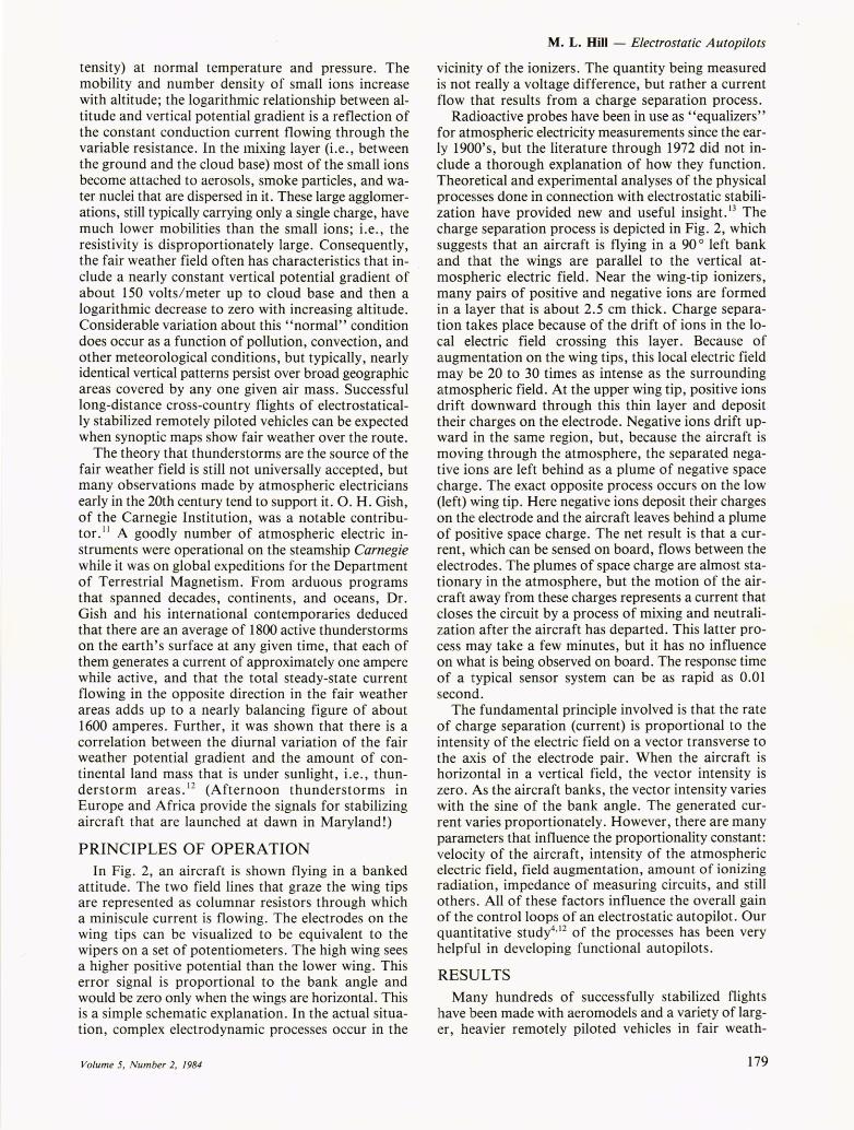
A short discussion of the phenomena would be an appropriate accompaniment to my article, "A Closed Course Distance Record for Powered Radio­Controlled Aeromodels" in this issue, especially with respect to the difficulties that were encountered near thunderstorms during the record flight. Actually, an electrostatically stabilized aeromodel, when it is fly­ing near a thunderstorm, becomes an instrument that is sensitive to a complex set of physical processes, i.e., aerodynamics of the vehicle, electromechanics of au­topilots, convection and turbulence, precipitation, electrification of cloud particles, and formation of in­tense electric fields in the surrounding space. Visual observation of the maneuvering instrument is infor­mative but, at best, it is a highly qualitative technique. However, I believe that a well-instrumented remotely piloted vehicle capable of penetrating thunderstorms could produce specific quantitative data that would be quite useful toward resolving some long-standing dis­agreements that still exist in theories about thunder­storm electrification.

177

M. L. Hill - Electrostatic Autopilots

ATMOSPHERIC ELECTRICITY

The literature on characteristics of atmospheric elec­tric fields is voluminous. A two-volume treatise by Israee'lO lists more than 1000 references. Atmospheric electricians use the term "fair weather field" to iden­tify the kinds of electric fields that are usually present in areas free of thunderstorms and other disturbances. The term "normal electric field" would perhaps be more appropriate to use in connection with electrostat­ic autopilots because similar characteristics are pres­ent during at least some kinds of rain and snow storms.

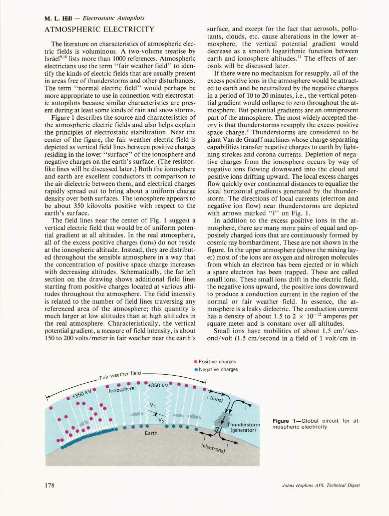
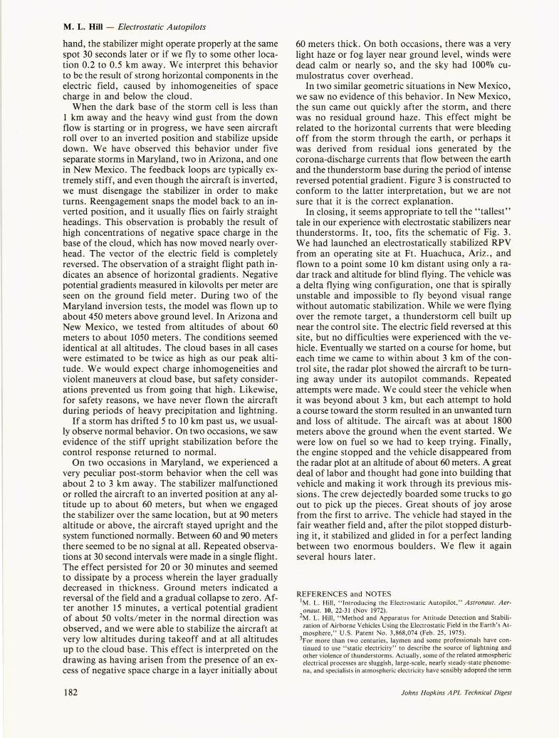
Figure 1 describes the source and characteristics of the atmospheric electric fields and also helps explain the principles of electrostatic stabilization. Near the center of the figure, the fair weather electric field is depicted as vertical field lines between positive charges residing in the lower "surface" of the ionosphere and negative charges on the earth's surface. (The resistor­like lines will be discussed later.) Both the ionosphere and earth are excellent conductors in comparison to the air dielectric between them, and electrical charges rapidly spread out to bring about a uniform charge density over both surfaces. The ionosphere appears to be about 350 kilovolts positive with respect to the earth's surface.

The field lines near the center of Fig. 1 suggest a vertical electric field that would be of uniform poten­tial gradient at all altitudes. In the real atmosphere, all of the excess positive charges (ions) do not reside at the ionospheric altitude. Instead, they are distribut­ed throughout the sensible atmosphere in a way that the concentration of positive space charge increases with decreasing altitudes. Schematically, the far left section on the drawing shows additional field lines starting from positive charges located at various alti­tudes throughout the atmosphere. The field intensity is related to the number of field lines traversing any referenced area of the atmosphere; this quantity is much larger at low altitudes than at high altitudes in the real atmosphere. Characteristically, the vertical potential gradient, a measure of field intensity, is about 150 to 200 volts/meter in fair weather near the earth's

surface, and except for the fact that aerosols, pollu­tants, clouds, etc. cause alterations in the lower at­mosphere, the vertical potential gradient would decrease as a smooth logarithmic function between earth and ionosphere altitudes. II The effects of aer­osols will be discussed later.

If there were no mechanism for resupply, all of the excess positive ions in the atmosphere would be attract­ed to earth and be neutralized by the negative charges in a period of 10 to 20 minutes, i.e., the vertical poten­tial gradient would collapse to zero throughout the at­mosphere. But potential gradients are an omnipresent part of the atmosphere. The most widely accepted the­ory is that thunderstorms resupply the excess positive space charge. 8 Thunderstorms are considered to be giant Van de Graaff machines whose charge-separating capabilities transfer negative charges to earth by light­ning strokes and corona currents. Depletion of nega­tive charges from the ionosphere occurs by way of negative ions flowing downward into the cloud and positive ions drifting upward. The local excess charges flow quickly over continental distances to equalize the local horizontal gradients generated by the thunder­storm. The directions of local currents (electron and negative ion flow) near thunderstorms are depicted with arrows marked "i" on Fig. 1.

In addition to the excess positive ions in the at­mosphere, there are many more pairs of equal and op­positely charged ions that are continuously formed by cosmic ray bombardment. These are not shown in the figure. In the upper atmosphere (above the mixing lay­er) most of the ions are oxygen and nitrogen molecules from which an electron has been ejected or in which a spare electron has been trapped. These are called small ions. These small ions drift in the electric field, the negative ions upward, the positive ions downward to produce a conduction current in the region of the normal or fair weather field. In essence, the at­mosphere is a leaky dielectric. The conduction current has a density of about 1.5 to 2 x 10- 12 amperes per square meter and is constant over all altitudes.

Small ions have mobilities of about 1.5 cm2/sec­ond/volt (1.5 cm/second in a field of 1 volt/cm in-

• Posit ive charges

. d • Negative charges . .• 'eather flel ~ faIr V'

~ •• • • · +350kV· ••• '\J • Ionosphere • 4 'i:>() y..

• ~'3 i (ions) ~ •• • • • • i

• •• • • • ·1 I Thunderstorm

• y~erator)

(elect I rOnS)

Earth

178

Figure 1-Global circuit for at­mospheric electricity .

Johns Hopkins A PL Technical Digest

tensity) at normal temperature and pressure. The mobility and number density of small ions increase with altitude; the logarithmic relationship between al­titude and vertical potential gradient is a reflection of the constant conduction current flowing through the variable resistance. In the mixing layer (i.e., between the ground and the cloud base) most of the small ions become attached to aerosols, smoke particles, and wa­ter nuclei that are dispersed in it. These large agglomer­ations, still typically carrying only a single charge, have much lower mobilities than the small ions; i.e., the resistivity is disproportionately large. Consequently, the fair weather field often has characteristics that in­clude a nearly constant vertical potential gradient of about 150 volts/meter up to cloud base and then a logarithmic decrease to zero with increasing altitude. Considerable variation about this' 'normal" condition does occur as a function of pollution, convection, and other meteorological conditions, but typically, nearly identical vertical patterns persist over broad geographic areas covered by anyone given air mass. Successful long-distance cross-country flights of electrostatical­ly stabilized remotely piloted vehicles can be expected when synoptic maps show fair weather over the route.

The theory that thunderstorms are the source of the fair weather field is still not universally accepted, but many observations made by atmospheric electricians early in the 20th century tend to support it. O. H. Gish, of the Carnegie Institution, was a notable contribu­tor. II A goodly number of atmospheric electric in­struments were operational on the steamship Carnegie while it was on global expeditions for the Department of Terrestrial Magnetism. From arduous programs that spanned decades, continents, and oceans, Dr. Gish and his international contemporaries deduced that there are an average of 1800 active thunderstorms on the earth's surface at any given time, that each of them generates a current of approximately one ampere while active, and that the total steady-state current flowing in the opposite direction in the fair weather areas adds up to a nearly balancing figure of about 1600 amperes. Further, it was shown that there is a correlation between the diurnal variation of the fair weather potential gradient and the amount of con­tinental land mass that is under sunlight, i.e., thun­derstorm areas. 12 (Afternoon thunderstorms in Europe and Africa provide the signals for stabilizing aircraft that are launched at dawn in Maryland!)

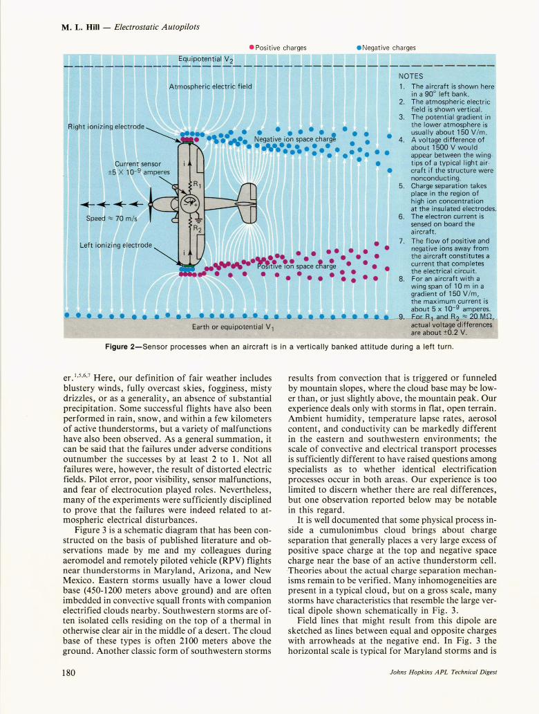
PRINCIPLES OF OPERATION In Fig. 2, an aircraft is shown flying in a banked

attitude. The two field lines that graze the wing tips are represented as columnar resistors through which a miniscule current is flowing. The electrodes on the wing tips can be visualized to be equivalent to the wipers on a set of potentiometers. The high wing sees a higher positive potential than the lower wing. This error signal is proportional to the bank angle and would be zero only when the wings are horizontal. This is a simple schematic explanation. In the actual situa­tion, complex electrodynamic processes occur in the

Volume 5, Number 2, 1984

M. L. Hill - Electrostatic Autopilots

vicinity of the ionizers. The quantity being measured is not really a voltage difference, but rather a current flow that results from a charge separation process.

Radioactive probes have been in use as "equalizers" for atmospheric electricity measurements since the ear­ly 1900's, but the literature through 1972 did not in­clude a thorough explanation of how they function. Theoretical and experimental analyses of the physical processes done in connection with electrostatic stabili­zation have provided new and useful insight. 13 The charge separation process is depicted in Fig. 2, which suggests that an aircraft is flying in a 90 0 left bank and that the wings are parallel to the vertical at­mospheric electric field. Near the wing-tip ionizers, many pairs of positive and negative ions are formed in a layer that is about 2.5 cm thick. Charge separa­tion takes place because of the drift of ions in the lo­cal electric field crossing this layer. Because of augmentation on the wing tips, this local electric field may be 20 to 30 times as intense as the surrounding atmospheric field. At the upper wing tip, positive ions drift downward through this thin layer and deposit their charges on the electrode. Negative ions drift up­ward in the same region, but, because the aircraft is moving through the atmosphere, the separated nega­tive ions are left behind as a plume of negative space charge. The exact opposite process occurs on the low (left) wing tip. Here negative ions deposit their charges on the electrode and the aircraft leaves behind a plume of positive space charge. The net result is that a cur­rent, which can be sensed on board, flows between the electrodes. The plumes of space charge are almost sta­tionary in the atmosphere, but the motion of the air­craft away from these charges represents a current that closes the circuit by a process of mixing and neutrali­zation after the aircraft has departed. This latter pro­cess may take a few minutes, but it has no influence on what is being observed on board. The response time of a typical sensor system can be as rapid as 0.01 second.

The fundamental principle involved is that the rate of charge separation (current) is proportional to the intensity of the electric field on a vector transverse to the axis of the electrode pair. When the aircraft is horizontal in a vertical field, the vector intensity is zero. As the aircraft banks, the vector intensity varies with the sine of the bank angle. The generated cur­rent varies proportionately. However, there are many parameters that influence the proportionality constant: velocity of the aircraft, intensity of the atmospheric electric field, field augmentation, amount of ionizing radiation, impedance of measuring circuits, and still others. All of these factors influence the overall gain of the control loops of an electrostatic autopilot. Our quantitative study4,12 of the processes has been very helpful in developing functional autopilots.

RESULTS Many hundreds of successfully stabilized flights

have been made with aero models and a variety of larg­er, heavier remotely piloted vehicles in fair weath-

179

M. L. Hill - Electrostatic Autopilots

• Positive charges . Negative charges

Equ ipotential V 2

Atmospheric electric field

Right ionizing electrode • • • • • • •• • •

Speed:::::: 70 mls

.... . -----.-.. Earth or equipotential V 1

• • • • •

• •

NOTES

1.

2.

3.

4 .

5.

6.

7 .

8.

The aircraft is shown here in a 90° left bank. The atmospheric electric field is shown vertical. The potential gradient in the lower atmosphere is usually about 150 V 1m . A voltage difference of about 1500 V would appear between the wing­tips of a typical light air­craft if the structure were nonconducting. Charge separation takes place in the region of high ion concentration at the insulated electrodes. The electron current is sensed on board the aircraft. The flow of positive and negative ions away from the aircraft constitutes a current that completes the electrical circuit. For an aircraft with a wing span of 10 m in a gradient of 150 V 1m, the maximum current is about 5 x 10- 9 amperes.

-e e 9. F.Dr,B-l_and Rz :::::: 20 Mil, _ actual voltage differences are about ±0.2 V.

Figure 2-Sensor processes when an aircraft is in a vertically banked attitude during a left turn.

er. 1,5,6,7 Here, our definition of fair weather includes blustery winds, fully overcast skies, fogginess, misty drizzles, or as a generality, an absence of substantial precipitation. Some successful flights have also been performed in rain, snow, and within a few kilometers of active thunderstorms, but a variety of malfunctions have also been observed. As a general summation, it can be said that the failures under adverse conditions outnumber the successes by at least 2 to 1. Not all failures were, however, the result of distorted electric fields. Pilot error, poor visibility, sensor malfunctions, and fear of electrocution played roles. Nevertheless, many of the experiments were sufficiently disciplined to prove that the failures were indeed related to at­mospheric electrical disturbances.

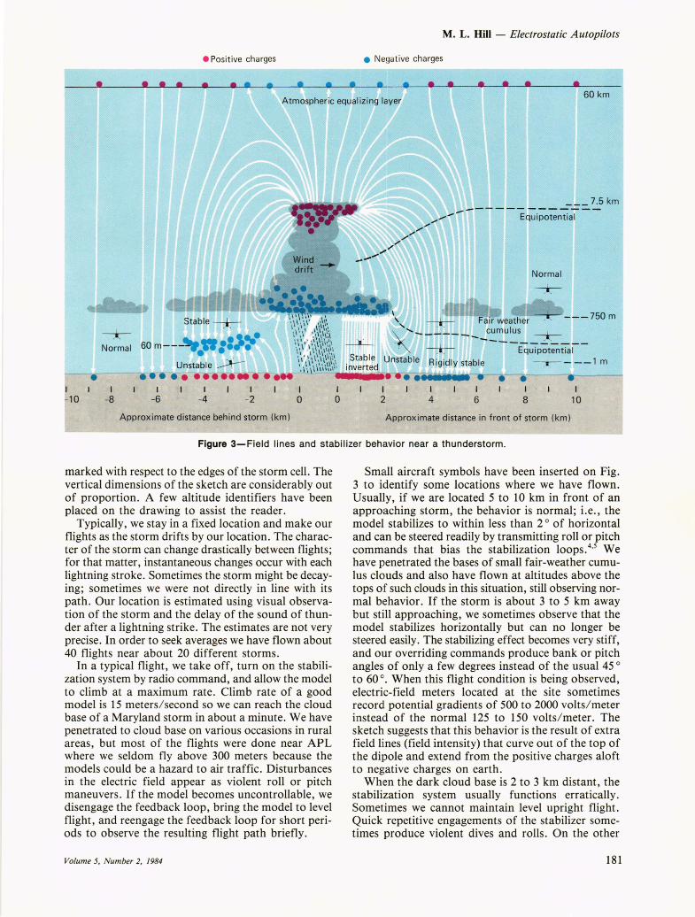
Figure 3 is a schematic diagram that has been con­structed on the basis of published literature and ob­servations made by me and my colleagues during aeromodel and remotely piloted vehicle (RPV) flights near thunderstorms in Maryland, Arizona, and New Mexico. Eastern storms usually have a lower cloud base (450-1200 meters above ground) and are often imbedded in convective squall fronts with companion electrified clouds nearby. Southwestern storms are of­ten isolated cells residing on the top of a thermal in otherwise clear air in the middle of a desert. The cloud base of these types is often 2100 meters above the ground. Another classic form of southwestern storms

180

results from convection that is triggered or funneled by mountain slopes, where the cloud base may be low­er than, or just slightly above, the mountain peak. Our experience deals only with storms in flat, open terrain. Ambient humidity, temperature lapse rates, aerosol content, and conductivity can be markedly different in the eastern and southwestern environments; the scale of convective and electrical transport processes is sufficiently different to have raised questions among specialists as to whether identical electrification processes occur in both areas. Our experience is too limited to discern whether there are real differences, but one observation reported below may be notable in this regard.

It is well documented that some physical process in­side a cumulonimbus cloud brings about charge separation that generally places a very large excess of positive space charge at the top and negative space charge near the base of an active thunderstorm cell. Theories about the actual charge separation mechan­isms remain to be verified. Many inhomogeneities are present in a typical cloud, but on a gross scale, many storms have characteristics that resemble the large ver­tical dipole shown schematically in Fig. 3.

Field lines that might result from this dipole are sketched as lines between equal and opposite charges with arrowheads at the negative end. In Fig. 3 the horizontal scale is typical for Maryland storms and is

Johns Hopkins APL Technical Digest

M. L. Hill - Electrostatic Autopilots

• Posit ive charges • Negative charges

• • • • • • • • • • • • • • • • • Atmospheric equal izing layer

60 km

I -10

I I -8 -6

I -4

I -2

Approx imate distance beh ind storm (km)

I o

Normal

'I;: ~ Fair weather =+---- 750 m ~ ...... __ ~~ ___ cumulus -+-

~ --+- ----EQ~P~t~~I-. Stable Unstable Rigidly stable - -t- - - - 1 m Inverted .. I -. .-... .... ....-• .......--. -.----

I I I I I I I I I o 2 4 6 8 10

Approximate distance in front of storm (km)

Figure 3-Field lines and stabilizer behavior near a thunderstorm.

marked with respect to the edges of the storm cell . The vertical dimensions of the sketch are considerably out of proportion. A few altitude identifiers have been placed on the drawing to assist the reader.

Typically, we stay in a fixed location and make our flights as the storm drifts by our location. The charac­ter of the storm can change drastically between flights; for that matter, instantaneous changes occur with each lightning stroke. Sometimes the storm might be decay­ing; sometimes we were not directly in line with its path. Our location is estimated using visual observa­tion of the storm and the delay of the sound of thun­der after a lightning strike. The estimates are not very precise. In order to seek averages we have flown about 40 flights near about 20 different storms.

In a typical flight, we take off, turn on the stabili­zation system by radio command, and allow the model to climb at a maximum rate. Climb rate of a good model is 15 meters/ second so we can reach the cloud base of a Maryland storm in about a minute. We have penetrated to cloud base on various occasions in rural areas, but most of the flights were done near APL where we seldom fly above 300 meters because the models could be a hazard to air traffic. Disturbances in the electric field appear as violent roll or pitch maneuvers. If the model becomes uncontrollable, we disengage the feedback loop, bring the model to level flight, and reengage the feedback loop for short peri­ods to observe the resulting flight path briefly.

Volume 5, Number 2, 1984

Small aircraft symbols have been inserted on Fig. 3 to identify some locations where we have flown. Usually, if we are located 5 to 10 km in front of an approaching storm, the behavior is normal; i.e., the model stabilizes to within less than 2 ° of horizontal and can be steered readily by transmitting roll or pitch commands that bias the stabilization 100ps.4.5 We have penetrated the bases of small fair-weather cumu­lus clouds and also have flown at altitudes above the tops of such clouds in this situation, still observing nor­mal behavior. If the storm is about 3 to 5 km away but still approaching, we sometimes observe that the model stabilizes horizontally but can no longer be steered easily. The stabilizing effect becomes very stiff, and our overriding commands produce bank or pitch angles of only a few degrees instead of the usual 45 ° to 60 o . When this flight condition is being observed, electric-field meters located at the site sometimes record potential gradients of 500 to 2000 volts/meter instead of the normal 125 to 150 volts/meter. The sketch suggests that this behavior is the result of extra field lines (field intensity) that curve out of the top of the dipole and extend from the positive charges aloft to negative charges on earth.

When the dark cloud base is 2 to 3 km distant, the stabilization system usually functions erratically. Sometimes we cannot maintain level upright flight. Quick repetitive engagements of the stabilizer some­times produce violent dives and rolls. On the other

181

M. L. Hill - Electrostatic Autopilots

hand, the stabilizer might operate properly at the same spot 30 seconds later or if we fly to some other loca­tion 0.2 to 0.5 km away. We interpret this behavior to be the result of strong horizontal components in the electric field, caused by inhomogeneities of space charge in and below the cloud.

When the dark base of the storm cell is less than 1 km away and the heavy wind gust from the down flow is starting or in progress, we have seen aircraft roll over to an inverted position and stabilize upside down. We have observed this behavior under five separate storms in Maryland, two in Arizona, and one in New Mexico. The feedback loops are typically ex­tremely stiff, and even though the aircraft is inverted, we must disengage the stabilizer in order to make turns. Reengagement snaps the model back to an in­verted position, and it usually flies on fairly straight headings. This observation is probably the result of high concentrations of negative space charge in the base of the cloud, which has now moved nearly over­head. The vector of the electric field is completely reversed. The observation of a straight flight path in­dicates an absence of horizontal gradients. Negative potential gradients measured in kilovolts per meter are seen on the ground field meter. During two of the Maryland inversion tests , the model was flown up to about 450 meters above ground level. In Arizona and New Mexico, we tested from altitudes of about 60 meters to about 1050 meters . The conditions seemed identical at all altitudes. The cloud bases in all cases were estimated to be twice as high as our peak alti­tude. We would expect charge inhomogeneities and violent maneuvers at cloud base, but safety consider­ations prevented us from going that high. Likewise, for safety reasons, we have never flown the aircraft during periods of heavy precipitation and lightning.

If a storm has drifted 5 to 10 km past us, we usual­ly observe normal behavior. On two occasions, we saw evidence of the stiff upright stabilization before the control response returned to normal.

On two occasions in Maryland, we experienced a very peculiar post-storm behavior when the cell was about 2 to 3 km away. The stabilizer malfunctioned or rolled the aircraft to an inverted position at any al­titude up to about 60 meters, but when we engaged the stabilizer over the same location, but at 90 meters altitude or above, the aircraft stayed upright and the system functioned normally. Between 60 and 90 meters there seemed to be no signal at all. Repeated observa­tions at 30 second intervals were made in a single flight. The effect persisted for 20 or 30 minutes and seemed to dissipate by a process wherein the layer gradually decreased in thickness. Ground meters indicated a reversal of the field and a gradual collapse to zero. Af­ter another 15 minutes, a vertical potential gradient of about 50 volts/ meter in the normal direction was observed, and we were able to stabilize the aircraft at very low altitudes during takeoff and at all altitudes up to the cloud base. This effect is interpreted on the drawing as having arisen from the presence of an ex­cess of negative space charge in a layer initially about

182

60 meters thick. On both occasions, there was a very light haze or fog layer near ground level, winds were dead calm or nearly so, and the sky had 100070 cu­mulostratus cover overhead.

In two similar geometric situations in New Mexico, we saw no evidence of this behavior. In New Mexico, the sun came out quickly after the storm, and there was no residual ground haze. This effect might be related to the horizontal currents that were bleeding off from the storm through the earth, or perhaps it was derived from residual ions generated by the corona-discharge currents that flow between the earth and the thunderstorm base during the period of intense reversed potential gradient. Figure 3 is constructed to conform to the latter interpretation, but we are not sure that it is the correct explanation.

In closing, it seems appropriate to tell the' 'tallest" tale in our experience with electrostatic stabilizers near thunderstorms. It, too, fits the schematic of Fig. 3. We had launched an electrostatically stabilized RPV from an operating site at Ft. Huachuca, Ariz ., and flown to a point some 10 km distant using only a ra­dar track and altitude for blind flying. The vehicle was a delta flying wing configuration, one that is spirally unstable and impossible to fly beyond visual range without automatic stabilization. While we were flying over the remote target, a thunderstorm cell built up near the control site. The electric field reversed at this site, but no difficulties were experienced with the ve­hicle . Eventually we started on a course for home, but each time we came to within about 3 km of the con­trol site, the radar plot showed the aircraft to be turn­ing away under its autopilot commands. Repeated attempts were made. We could steer the vehicle when it was beyond about 3 km, but each attempt to hold a course toward the storm resulted in an unwanted turn and loss of altitude. The aircaft was at about 1800 meters above the ground when the event started. We were low on fuel so we had to keep trying. Finally, the engine stopped and the vehicle disappeared from the radar plot at an altitude of about 60 meters. A great deal of labor and thought had gone into building that vehicle and making it work through its previous mis­sions. The crew dejectedly boarded some trucks to go out to pick up the pieces. Great shouts of joy arose from the first to arrive. The vehicle had stayed in the fair weather field and, after the pilot stopped disturb­ing it, it stabilized and glided in for a perfect landing between two enormous boulders. We flew it again several hours later.

REFERENCES and NOTES 1M. L. Hill , " Introducing the Electrostatic Autopi lot," Astronaut. Aer­onaut. 10, 22-31 (Nov 1972) .

2M. L. Hill , "Method and Apparatus for Attitude Detection and Stabi li­zation of Airborne Vehicles Using the Electrostatic Field in the Earth's At­mosphere," U.S. Patent No. 3,868,074 (Feb. 25, 1975).

3For more than two centuries, laymen and some professionals have con­tinued to use "static electricity" to describe the source of lightning and other violence of thu nderstorms. Actually, some of the related atmospheric electrical processes are sluggish, large-scale, nearly steady-state phenome­na, and specialists in atmospheric electricity have sensibly adopted the term

Johns Hopkins A PL Technical Digest

"quasi-electrostatic" to classify electrical properties of the atmosphere that have outward appearances of being essentially static. Proper protocol would demand that the present concept be called "quasi-electrostatic aircraft stabilization," but one can hardly expect such cumbersome obliqueness to be popular in aviation circles where speed in getting to the point has always been a classic objective.

4M . L. Hill and T. R. Whyte, Investigations Related to the Use of At­mospheric Electric Fields for Aircraft and RPV Stabilization, JHU/ APL TG 1280 (Jun 1975).

5M . L. Hill, "Design and Performance of Electrostatically Stabilized Del­ta Plan form Mini RPVs," in Conf. Proc., Military Electronics Defense Exposition, Wiesbaden, Germany, Interavia SA, Geneva, Switzerland, pp. 847-861 (Oct 1977).

6M . L. Hill, T. R. Whyte, R. O. Weiss, R. Rubio, and M. Isquierdo, "Use of Atmospheric Electric Fields for Vertical Stabilization and Terrain Avoidance," in Proc. AIAA Guidance and Control Conf., Albuquerque (AIAA paper 81-1848) (19-21 Aug 1981).

7M. L. Hill, "World Endurance Record for Radio Controlled Aeromodels," Johns Hopkins APL Tech. Dig. 3, 81-89 (1982).

8M. L. Hill, "Designing a Mini-RPV for a World Endurance Record," As­tronaut. Aeronaut. 20,47-54 (Nov 1982).

9H . Israel, Atmospheric Electricity, Vol. I, Fundamentals, Conductivity, Ions, Israel Program for Scientific Translation Ltd ., National Science Foun­dation (available from U .S. Department of Commerce) NTIS TT67-513941I, Washington , D.C. (1971).

Volume 5, Number 2, 1984

M. L. Hill - Electrostatic Autopilots

·IOH . Israel, Atmospheric Electricity, Vol. II, Fields, Charges, Currents, Is­rael Program for Scientific Translation Ltd., National Science Founda­tion (available from U.S. Department of Commerce) NTIS TT67-5139412, Washington, D.C. (1973).

110. H. Gish, "Evaluation and Interpretation of the Columnar Resistance of the Atmosphere," Terr. Magn. Atmos. Electr.49, 159 (1944).

12It is awesome to realize that men like Gish could assemble such complex global concepts in the days when scientists went to sea for months at a time to gather fewer data points than a satellite can deliver in a few minutes today. Dr. Merle A. Tuve, APL's first director, was at the Carnegie Insti­tution's Department of Terrestrial Magnetism at least part of the time while these global circuit concepts were being developed. Amidst a conference of atmospheric electricians, Dr. Tuve rose and commented, "The trouble with atmospheric electricity is that the stuff has been under study for nearly two centuries and there is yet to be an invention that is a help to humani­ty." Dr. R. E. Gibson knew both Dr. Gish and Dr. Tuve quite well. It is a pleasure to recall a conversation where Dr. Gibson said "Dr. Tuve's comment was in all likelihood, a lighthearted one aimed at stimulating the scientists to focus on goals," adding, with his inimitable twinkle and ac­cent, "He was quite good at it, you know ."

13M . L. Hill and W. A. Hoppel, "Effects of Velocity and Other Physical Variables on the Currents and Potentials Generated by Radioactive Col­lectors in Electric Field Measurements," in Proc. Fifth International Conf. on Atmospheric Electricity, Dietrich Steinkopff Verlag, Darmstadt, pp. 238-248 (1977).

183