elementary particle physics lecture notes 2013-14 -...
TRANSCRIPT

Elementary Particle Physics Lecture Notes 2013-14
Bobby Samir Acharya
March 4, 2014
1

Resources
Books:Halzen-Martin: Quarks and Leptons: An Introductory Course in Modern Elementary Particle
PhysicsandKane: Modern Elementary Particle PhysicsandThompson: Modern Particle Physics
Will mainly use Halzen-Martin, but Kane and Thompson are also very useful texts.The known properties of the Standard Model particles and all known particles are listed in the
Particle Data Group book: http://pdg.lbl.gov/2012/listings/contents listings.htmlThis is an invaluable resource for particle physicists!
2

Particle Physics. Weeks 1 and 2
Brief Review of Week 1: (refer to the slides for a reminder. Chapter1 of Halzen-Martin and/or Thompson is also a good summary of sometopics we discussed.)
In Week 1 we covered:
Some evidence for the classification of matter into particles: the peri-odic table, the discovery of the electron and the discovery of the nucleus.
We connected particle physics to the Universe at large: We noted thefact that the ∼ 1011 stars in the galaxy look alike to first approximation.Similarly, the ∼ 1011 galaxies are also alike to first approximation, im-plying that there are roughly 1011 × 1011 = 1022 stars, all approximatelylike our sun, in the observable Universe. Since our sun’s mass is approx-imately 1030 kg and we know it is composed of atoms (e.g. H and He
and others) and that an atom has a mass of roughly 10−27 kg, we learnthat there are approximately 1011×1011×1030×1027 = 1079 protons andneutrons in the Universe!. All of these are described by particle physics.
We introduced the Standard Model of Particle Physics for the firsttime: we described the three families (or generations or flavours) of quarksand leptons. We discussed their properties such as electric charge andmass. We pointed out the huge range of masses from the lightest chargedparticle (the electron) to the heaviest one (the top quark). These span sixorders of magnitude. If we consider that the neutral fermion masses (theneutrinos) have to be less than about 1 eV/c2 (though we will use naturalunits with c = 1), then the masses span at least 12 orders of magnitude(an order of magnitude is essentially adding an additional digit, so thenumber 130 is an order of magnitude larger than the number 16; similarly2456 is two orders of magnitude smaller than 355573.)
We introduced the strong, weak and electromagnetic interactions; theseare the three forces which govern the behaviour of matter at distancescales short enough (equivalently energy scales high enough) that gravity
3
is sub-dominant. We described the forces as being via the exchangeof gauge bosons (the photon, gluons, W±, Z) and introduced the basicFeynman diagrams (containing two fermions and one boson) which givesthe basic structure of the Standard Model. We described which particlesparticipate in the three forces. All electrically chared particles participatein electromagnetism, so that means all the fermions except neutrinos.The leptons do not participate in strong interactions, only the quarksand gluons do this. All the particles participate in the weak interactionsinvolving the W and Z bosons. (Note: later we will note that fermionscan be ”left-handed” or ”right-handed” so that only left handed particles(and right handed anti-particles) participate in the interactions with W -bosons.). By putting together these basic Feynman diagrams we cancreate more complicated ones and these are the processes described bythe Standard Model.
Each interaction (strong, weak, electromagnetic) is thus associatedwith a simple Feynman diagram; at the vertex of the diagram is assigneda ”charge”. When the boson is the photon, this is the electromagneticinteraction and the ”charge” is actually the electric charge, e. For thestrong and weak interactions it is a different charge and is denoted g3 forthe strong interaction and g2 for the weak interaction with W -bosons.For the weak interactions involving the Z-boson we will later see thatthe strength is given by a particular combination of e and g2.
We mentioned that the charges actually are not constants, rather theydepend upon the energy scale of the process that a particular Feynmandiagram is describing. Consider the following two diagrams taken fromHalzen-Martin. An electron is not ”just an electron”. It is continuallyradiating photons which convert into e+e− pairs. An electron is thussurrounded by a ”virtual cloud” of electron/positron pairs (see next dia-gram). The positrons in the cloud will tend to be closer to the originalelectron as they have opposite charge. Hence, the cloud is polarised. Thisaffects what we mean by charge in a distance/energy dependent way.
4

We can measure the electron charge by taking a test charge and mea-suring the force it experiences. Clearly, the result depends upon how closethe test charge is to the electron cloud, as the next figure illustrates. Thepositrons effectively screen the electron from the test charge: a photonwhich is exchanged between the positive test charge and a cloud positrongives a ”repulsive” contribution to the overall force (which is attractive);the cloud electrons also contribute to this effect, but because they arefarther out there is a smaller chance that the photons will interact withthem so the effect is smaller. As the test charge is brought closer, theeffective charge increases as the screening effect becomes less and less rel-evant. This results in a distance (equivalently energy) dependent charge,which is larger at shorter distances or higher energies.
5

In the case of the strong interactions (described by quantum chromo-dynamics or QCD) the story is similar but with a different result. Thisis illustrated in the other part of figure 1.5. In the strong interactions,gluons can interact with themselves (cf electromagnetism where photonscannot self-interact). This leads to additional contributions to the effec-tive charge which in fact leads to an energy dependance of the chargewhich is opposite to that in quantum electrodynamics (QED). In QCDthe strength of the interaction i.e. the charge increases with distance ordecreases with energy – so that asymptotically at arbitrarily high ener-gies the charge goes to zero. This is known as asymptotic freedom. Theunderstanding of this phenomenon led to a Nobel prize in physics forGross, Politzer and Wilczek in 2004. As a consequence, at low energiesit is not possible to directly observe quarks or gluons: the strong interac-tion is so strong that it binds them into bound states known collectivelyas ”hadrons”. One of these, the proton, is long lived. The rest of them,though, do not have long lifetimes: they quickly decay due to the electro-
6

magnetic and weak interactions that their constituents also participatein.
The Large Hadron ColliderWe gave an overview of the Large Hadron Collider. Set in a roughly
circular, 27 km diameter tunnel, about 100 m below ground, the LHCis the world’s largest machine. It is also the world’s most energetic andpowerful particle collider. Powerful superconducting magnets and electricfields are used to accelerate charged particles (usually protons, but alsolead ions) around the LHC ring in both directions. The two counterrotating particle beams are made to collide at four interaction pointsaround the ring. Surrounding each interaction point are different particledetectors, designed to measure the results of proton-proton (and other)collisions. The LHC is designed to collide protons at a centre-of-massenergy
√s of 14 TeV = 14 ×1012 eV. It first started operation (more
than 20 years after its conception) in 2010. It has successfully run in2011 at
√s=7 TeV and in 2012 at
√s=8 TeV. For most of 2013 and 2014
it will be undergoing upgrades in order to ramp up to the design energy.
High energy is one key property that is necessary for a successful LHC.The collider also has a very high luminosity. The higher the luminositythe greater the number of collisions between the particle beams will takeplace. This is proportional to the number of protons in each of the collid-ing beams and inversely proportional to the effective area over which thebeams are made to collide. Hence, luminosity is measured in units of in-verse area cm−2 or the instantaneous luminosity is given in cm−2s−1. Thedesign luminosity of the LHC is about 1034cm−2s−1 (or about 1041cm−2
per year) and last year it was running pretty close to that. High energyis required because we are hoping to produce new particles with a largemass in the collisions and this can’t be done if there isn’t enough energy.High luminosity is required because the production of new particles is arare process (otherwise we may have seen them already!) so the largerthe number of collisions the greater the probability of producing a newparticle. For instance, a Higgs boson is produced about once for everybillion collisions at the LHC.
7

Protons are not elementary particles, but rather ”large”, complicatedbound states of quarks and gluons tightly bound together by the stronginteraction. One aim is to get the quarks or gluons from one proton beamto collide ”hard” with those of the other proton beam and produce in-teresting new particles. Colliding protons together is a bit like collidingcans of beans together at high energies to both create new flavours ofbeans in the process as well as understand which beans are in the cans.As a result, proton-proton collisions are ”quite messy” with hundreds ofparticles being produced in a given collision. The detectors which mea-sure the results of these collisions must therefore be quite sophisticated,comprehensive, versatile instruments capable of recording pretty muchanything that could conceivably be spat out of a proton-proton collision.
One of the main aims of the LHC projects was to prove or disprove theexistence of the Higgs boson. The theory of the Higgs boson goes back to1964 when Peter Higgs (who studied at King’s !) proposed a mechanismto give masses to gauge bosons. This mechanism was incorporated intowhat eventually became the Standard Model – and it is the interactionsof the fermions and the bosons with the Higgs boson which is responsiblefor the masses that those particles have. The proof (or disproof) of theexistence of the Higgs boson is thus paramount to our understandingof the nature of mass and goes a long way towards answering e.g. thequestion ”why is the mass of the electron about 0.5 MeV/c2 ?” andtowards asking about the nature of mass itself. Particle physicists havebeen looking for this particle for decades. Remarkably, after analysingdata collected in 2011 and 2012, the CMS (Compact Muon Solenoid)and ATLAS (A Toroidal LHC Apparatus) experiments at the CERNLHC have discovered a new particle with properties remarkably similarto that of the Higgs boson. Much work is now underway to measure thedetailed properties of this newly discovered particle to verify if it reallyis the Higgs boson or something else.
8

Natural Units and Dimensional AnalysisNatural units are a system of units which actually make thinking about
physics easier. This is because in these units energy and mass have thesame dimensions and these are inverse to the dimensions of lengths andtimes. In fact, in natural units any physical quantity will have dimensionsof mass to some power; equivalently it will have the dimension of lengthto the inverse power.
These units are defined by ”setting Planck’s constant ~ and the speedof light c to one. ” We put the previous statement in speech marksbecause the speed of light and ~ are not equal to one in a general unitsystem; however they are fundamental constants of nature. Hence youcan view the speed of light as a relationship between metres and seconds.In fact, in SI units metres are defined by ”the length of the path travelledby light in vacuum during a time interval of 1/299,792,458 of a second ”.Thus c can be viewed as a conversion factor between metres and seconds.
In natural units,
1 s = 299792458.. m (1)
which we will often approximate to
1 s = 3× 10⁸ m (2)
Similarly, Plancks constant (over 2π) which has the value
~ = 1.05457172534× 10⁻³⁴ Js (3)
can be thought of as a conversion factor between Joules and inverseseconds. This leads to the approximate relation
1 J ∼ 1034s−1 (4)
Since both ~ and c involve seconds, combining them allows us to con-vert between energy [E], 1/time [T ]−1 and 1/distance [L]−1.
One Joule can be expressed in electron volts as
9

1 eV = 1.602176..× 10−19 J (5)
so, ~ = 1 implies
~ = 1 ∼ 10−34J s ∼ 3× 10⁻²⁶J m ∼ 3× 10⁻²⁶ 1019
1.6..eV m ∼ 2× 10⁻⁷eV m
(6)
1 m ∼ 1
2× 10⁻⁷ eV(7)
which means that a distance of one metre is equivalent to an energyscale of 2× 10⁻⁷ eV. Larger distances correspond to smaller energies andvice-versa.
In natural units, the mass of the electron is about 0.5 MeV. This isthe inverse of a distance of 1
0.5MeV ∼ 4 × 10⁻¹³ m This is the Comp-ton wavelength of the electron. The mass of proton is about 0.94 GeV,corresponding to a length scale of order 2× 10⁻¹⁶ m. This is the charac-teristic size of a nucleus. The masses of the W -bosons, the Z-boson, thetop quark and (if confirmed at the LHC) the Higgs boson are of order100 GeV – corresponding to a distance of around 2×10⁻¹⁸ m. The LHCcollisions in 2012 took place at energies of 8 TeV = 8 thousand GeV – adistance scale of almost 10−20 m. This makes the LHC the world’s mostpowerful microscope.
10

Lorentz Invariance, Special Relativity and 4-vector notation
Einstein’s postulates of special relativity:
1. The speed of light is a constant, measured to have the same valueby all observers
2. The laws of physics are the same for all observers moving withconstant relative velocity to one another (i.e. in uniform relative motion).
If the relative motion between observers is along the x direction, then
t′ = γ(t− vx) (8)
x′ = γ(x− vt)y′ = y
z′ = z
where
γ =1√
1− v2(9)
The boost along the x-direction with velocity v mixes the space andtime coordinates x and t. A key fact about special relativity is that thequantity
L2 ≡ t2 − x2 − y2 − z2 (10)
is invariant under Lorentz transformations. In fact,
t′2 − x′2 − y′2 − z′2 = γ2(t2 − 2vx+ v2x2)− γ2(x2 − 2vt+ v2t2)− y2 − z2(11)
=1
1− v2 (t2 − x2)(1− v2)
= t2 − x2 − y2 − z2 = L2
The left and right hand side of this equation can be regarded as a mea-sure of spacetime length and are unchanged by Lorentz transformations
11

(note: the overall sign of the length is not important, we could have used−t2 + x2 + ...).
We can write this in a more compact form.Assemble the four space and time coordinates into a vector with four
components, a 4-vector and call this xµ.
xµ ≡
txyz
≡x0
x1
x2
x3
The invariant length can be thought of as a sort of dot product between
this vector and itself, but defined with some minus signs. In fact
L2 =(t x y z
)1 0 0 00 −1 0 00 0 −1 00 0 0 −1
tx
y
z
i.e.
L2 = (xµ)Tηxµ ≡ xµηµνxν (12)
where xµ is viewed as a vector multipling the matrix ηµν; η is knownas the Minkowski ”metric”:
ηµν ≡
1 0 0 00 −1 0 00 0 −1 00 0 0 −1
Note: η is denoted by g in Halzen-Martin.We often simplify life and omit the η by writing
L2 = xµxµ (13)
where, now, notice that the µ is a subscript on the first x. xµ is simply(xν)Tηµν and now the product between xµ and xµ is the usual dot product.
12
The space coordinates (x, y, z) ≡ xi are the components of a 3-vector.Another familiar 3-vector is the 3-momentum, pi ≡ (px, py, pz) which arethe components of an objects momentum in the three spatial directions.In the same way that the xi combine with another quantity t to forma 4-vector xµ, the 3-vector pi combines with another quantity to give a4-vector pµ – the 4-momentum. In this case, it is the energy of the objectwhich is p0:
pµ ≡
Epxpypz
≡p0
p1
p2
p3
The quantity,
M 2 = pµpµ = E2 − p2x − p2
y − p2z = E2 − |pi|2 (14)
is also Lorentz invariant, like L2. Hence it will be the same in allrelatively uniform frames. Consider now a (frame in which we have a)particle a rest. Being at rest, its momentum is zero, pi = 0. Hence
pµ ≡
E
000
=
m000
its energy is equal to its mass. Hence, in this frame,
M 2 = m2 (15)
but, since M 2 is Lorentz invariant, M 2 = m2 in all frames. Hence Mis known as the invariant mass. Therefore,
E2 = |pi|2 +m2 (16)
notice that, in the small velocity limit, pi → 0 and E ≈ m. In non-natural units this becomes E ≈ mc2, a famous equation but one whichis only approximately true.
The energy-momentum 4-vectors of a system are conserved in time:e.g. consider and initial state with two particles A and B with 4-vectors
13

pAµ and pBµ which interact, producing a final state with particles C andD. Energy-mometum conservation asserts that:
P µA + P µ
B = P µC + P µ
D (17)
where the lhs and rhs are both additions of two 4-vectors.In the case of a Higgs boson decaying into, say, two photons the initial
state is one particle (the Higgs boson) whereas the final state is twoparticles. If we label the Higgs boson as A and the two photons as Band C, at an LHC experiment we will measure the energy and momentaof each of the two photons. But conservation of energy and momentumimplies that:
P µA = P µ
B + P µC (18)
Therefore, we can reconstruct the energy and momentum of the Higgsby measuring the energy and momentum of the particles it decayed into.The mass of the Higgs boson mh is the invariant mass of P µ
A, thereforewe have:
m2h = P µ
APAµ = (P µB + P µ
C)(PBµ + PCµ) (19)
So we can measure the mass of the Higgs boson at the LHC eventhough the Higgs decayed very quickly.
14
From Schrodingers equation to Relativistic Quantum Theory
Non-relativistic Quantum Mechanics
Non-relativistic quantum mechanics is governed by Schrodingers equa-tion. This equation is simply an expression in waves/fields of the non-relativistic energy-momentum relation:
E =p2
2m(20)
If we substitute for E and p the differential operators:
E → i∂
∂tand pi → −i
∂
∂xi(21)
we get the free Schrodinger equation:
i∂Ψ
∂t+
1
2m
∂2Ψ
∂x2i
= 0 (22)
where we are acting with the equation on a function of space and timeΨ, called the wavefunction. Then
ρ = |Ψ|2 (23)
is the probability density and
ρd3x (24)
the probability of finding the particle in the infinitessimal volume ele-ment d3x.
For applications in which beams of particles interact/collide we willneed to calculate the ”flux density” of particles j passing out of somevolume V . The conservation of probability ρ asserts that the rate ofdecrease of the number of particles is equal to the flux coming out of asurface S surrounding the volume V :
− ∂
∂t
∫V
ρdV =
∫S
n.jdS =
∫V
∇.jdV (25)
15

n is just a unit normal vector to S and the last inequality is Stokestheorem. We therefore have a continuity equation:
∂ρ
∂t+∇.j = 0 (26)
Next we can get an expression for ∂ρ∂t by taking Schrodingers equa-
tion and multiplying on the left by −iΨ∗ and substracting this from thecomplex-conjugate of Schrodingers equation multiplied by −iΨ. Thisgives:
∂ρ
∂t=
i
2m(Ψ∗∇2Ψ−Ψ∇2Ψ∗) (27)
This implies that the probability flux density j is
j = − i
2m(Ψ∗∇Ψ−Ψ∇Ψ∗) (28)
A simple solution of the free Schrodinger equation is:
Ψ = Nei(pjxj−Et) = Neip
µxµ (29)
which describes a free particle with momentum pi ≡ p and energy E
(notice that the exponent is Lorentz invariant). This has
ρ = |N |2 and j =p
m|N |2 (30)
Relativistic Quantum Mechanics: the Klein-Gordon Equation
We can perform the same exercise with the relativistic E, p relation:
E2 = p2 +m2 (31)
This gives the Klein-Gordon equation,
−∂2φ
∂t2+∇2φ = m2φ (32)
φ is the wavefunction (or field) for a relativistic particle with mass m,energy E and momentum p. Again, we can multiply the equation by
16

−iφ∗ and substract this from the complex conjugate equation multipliedby −iφ to obtain ρ and j:
ρ = i(φ∗∂φ
∂t− φ∂φ
∗
∂t) (33)
and
j = −i(φ∗∇φ− φ∇φ∗) (34)
A free particle solution of the KG equation is again given by
φfree = Nei(pjxj−Et) = Neip
µxµ (35)
hence
ρ = 2E|N |2 and j = 2p|N |2 (36)
The KG equation is Lorentz invariant, since it can be written as
(∂ν∂ν +m2)φ = 0 (37)
and this suggests that ρ and j should combine into the four componentsof a 4-vector:
jµ ≡
ρ
j1
j2
j3
= −i(φ∗∂µφ− φ∂µφ∗) = 2pµ|N |2
The continuity equation can be written in the Lorentz invariant form
∂µjµ = 0 (38)
Substituting the free particle solution into the KG equation, we seethat we can have solutions for both signs of the square root:
E = ±√
p2 +m2 (39)
We need to interpret the negative energy solutions. Furthermore, thenegative energy solutions have negative probability density:
17

E < 0 , ρ < 0 (40)
Pauli and Weisskopf had the idea of multiplying jµ by the charge, e:
jµ −→ −ie(φ∗∂µφ− φ∂µφ∗) (41)
In this case ”negative ρ” can be associated with particles with theopposite charge.
The final interpretation of the negative energy solutions was given byFeynman and Stuckelberg who asserted: The negative energy particlesolutions are actually positive energy anti-particles. Moreover, if thelatter propagate forwards in time, the former are propagating backwardsin time. To see this, consider an electron of energy E, momentum p andcharge −e. It has
jµ(e−) = −2e|N |2(E,p) (42)
A positron, with the same E and p has
jµ(e+) = +2e|N |2(E,p) (43)
= −2e|N |2(−E,−p)
which is the same as that for an electron with energy −E and momen-tum −p.
This basically implies that the single particle wavefunction formalismdescribes both particles and antiparticles simultaneously. See Halzen-Martin 3.5 for some more details.
18

From Amplitudes to Cross-sections and Lifetimes.
Using basic quantum mechanics and the relativistic wave equation wehave seen that partice physics processes can be organised into Feynmandiagrams in which the probability per unit time per unit volume is relatedto the square of the amplitude.
For charged particles scattering by exchanging photons, the amplitudeis given by
Tfi = −i∫d4xjµ1 (x)
−1
q2 j2µ(x) (44)
Here, jµ1 is the current for one of the particles and j2µ the current forthe other. −1
q2 is the propagator of the photon which is exchanged betweenthem.
We derived the currents for both non-relativistic and relativistic parti-cles earlier. In the relativistic case, j2µ = −eNBND(pD + pB)µei(pD−pB).x.Putting this, and the analagous expression for the other current into theexpression for Tfi gives
Tfi = −iNANBNCND(2π)4δ4(pD + pC − pA − pB)M (45)
where
− iM = (ie(pA + pC)µ)(−igµνq2 )(ie(pB + pD)ν) (46)
M is simply the Feynman diagram translated into a mathematicalexpression, known as the invariant amplitude. M is intrinsically physical.The remaining factors in Tfi take care of a) the energy and momentumconservation of the process and b) the normalisation of the particle wavefunctions.
In particle physics experiments we measure quantities like the lifetimeof a decaying particle or the rate of production of particles from a colliderexperiment. We need to be able to calculate quantities like these, startingwith the invariant amplitude M for such a process.
19

1 Particle Decays
Consider a particle which decays into a number of other particles. e.g. aW -boson can decay into a positron and a neutrino, a neutron can decayas n → peνe, a muon decays as µ → eνµνe. These processes can bemeasured and we would like to understand what the Standard Modelpredicts for them.
In general, if the initial particle has some fixed energy and momen-tum, there are many possibilities for what the final state energies andmomenta could be for the particles produced in the decay. The initialparticle has a specified energy and momentum (obeying E2 = p2 +m2!),but, given this, there are many possible final state particle energies andmomenta. If we integrate over all of these possible final state energiesand momenta, taking into account energy and momentum conservation(which is enforced by the delta-function), we can obtain (for example)the lifetime of the particle.
Independent of the final state energies and momenta, there might bemany different combinations of particles that a given particle can de-cay into. For instance, a W -boson can decay into (e+, νe); (µ+, νµ); .......
20

Each possible combination of final state particles (which differ by their”charges”) contributes to the total lifetime. The branching ratio (orbranching fraction) for a particular final state combination of particles isthe (inverse of) the total lifetime of the particle divided by the averagelifetime for decaying into the given combination.
Recall (Fermi’s Golden rule) that gave us the probability per unit timefor a transition from one state to another. If the initial state is a particleand the final state the particles it decays into, this gives us the probabilityper unit time for the decay to occur.
Γ = 2π|M|2ρ(E) (47)
ρ(E) is the density of states. More about this in a moment. Γ is knownas the decay width of the particle. The lifetime of the particle is:
τ =1
Γ(48)
In natural units, ~ =1 = c and, hence, energies and masses can bemeasured in units of eV and distances and times in units of eV−1. Thusa lifetime has dimensions of [E]−1 = [M]−1 and Γ has dimensions of massi.e. [Γ] = [M].
1.1 Particle Number Density
Consider quantum mechanics in a finite region of space - a box with sidesof equal length L.
We require that the single particle, free particle wave function, e−ip.x
has well defined boundary conditions at the boundaries of the box i.e.when, x, y or z = L. For this we can impose periodic boundary conditionsso that the wave function is periodic at the boundaries:
Ψ(x, y, z) = Ψ(x+ L, y + L, z + L) (49)
This implies that
(px, py, pz) =2π
L(nx, ny, nz) (50)
21

where the ni are INTEGERS. The momentum of a single particle in abox is QUANTISED.
Hence, the number of states between px and px + dpx is L2πdpx.
Therefore, the number density of states for a single particle is:
dn =L3
(2π)3d3p =
V
(2π)3d3p (51)
1.2 The Lifetime of the Neutron
Though stable inside most atoms, a free neutron is unstable. It decaysinto a proton, an electron and an anti-neutrino:
n −→ pe−νe (52)
This is β-decay and also occurs within certain radioactive elements.The lifetime of the neutron at rest is about 900 seconds = 900 × 3× 108
m ≈ 900 × 3× 108 ×106eV−1 ≈ 2.7 × 10¹⁷eV−1 = 2.7 ×1026GeV−1.We will estimate the lifetime ignoring the masses of the electron and
neutrino. The mass difference between a neutron and proton is around1 MeV. The kinematics of this process is as follows. The energy of theneutron must equal that of the proton plus electron plus neutrino:
En = Ep + Ee + Eν (53)
If the initial neutron is at rest, En = mn and, since we ignore themasses of the e and ν we have that Ee = |pe| ≡ p and Eν = |pν| ≡ q.
22

The momentum of the proton is equal and opposite to the sum of themomenta of the electron and neutrino, so is completely fixed. Hence,when we integrate over the final state particles, we only need to integrateover the electron and neutrino momenta. We will define En − Ep to beE0, an energy of order 1 MeV.
Γ = 2π|M|2ρ = 2π
∫|M|2 d3p
(2π)3
d3q
(2π)3 (54)
where the∫
means we will integrate over p and q.A quick reminder about spherical polar coordinates is in order!
1.3 Spherical polar coordinates on the side
Consider the three space coordinates xi = (x, y, z). We can re-write thesein terms of two angles (θ, φ) and a radius r:
x = rsinθcosφ (55)
y = rsinθsinφ (56)
z = rcosθ (57)
where r > 0, 0 ≤ θ ≤ π, 0 ≤ φ ≤ 2π. Now, instead of specifying x, yand z to specify a particular point, we can specify r, θ and φ instead.This is a coordinate transformation. Note, that we can do this for thecomponents of any three-vector, e.g. momentum.
Notice that:
r = (x2 + y2 + z2)1/2 (58)
φ = tan−1(y/x) (59)
θ = cos−1(z/r) (60)
So, in particular, r = |xi|, the length of the vector.Important to note is how the integration measure gets transformed:
dxdydz −→ r2sinθdrdφdθ (61)
23

We can integrate over the two angles:∫r2dr
∫dφ
∫sinθdθ = 4πr2
∫dr (62)
So, the integral over space becomes equivalent to an integral over r:∫d3x = 4π
∫r2dr (63)
Similarly, instead of the 3-vector xi we could consider the 3-momentumpi: ∫
d3p = 4π
∫p2dp (64)
end of scholium on spherical polar coordinates. back to the density offinal states.
Now, back to neutron decay!Assuming the angular dependence of the matrix element is trivial, we
can replace d3p with 4πp2dp, and, similarly for q. Moreover, q = E0−Ee =E0 − p (since we ignore the electron mass), so there is no actual integralover q and we only have to integrate over p. Therefore, we have
Γ ≈∫ E0
0|M|2 (E0 − p)2
2π3 p2dp (65)
The integral over p is easy and the end result is:
Γ ≈ |M|2E5
0
60π3 (66)
Since Γ has dimensions of mass, dimensional analysis tells us that forthis process the dimension of |M|2 is mass−4.
Let us therefore relabel |M|2 as 1M4
∗, the goal being to estimate what
this mass M∗ is. Historically, M∗ is related to Fermi’s constant as GF ∼M−2∗ .
24
So, we now have:
Γ ≈ E50
M 4∗60π3 (67)
Since E0 is of order an MeV, we can write
Γ ≈ MeV
60π3
MeV4
M 4∗
(68)
The second factor is dimensionless. Since 60π3 ≈ 1860 ≈ 2000 we have
Γ ≈ 5× 10⁻⁴MeVMeV4
M 4∗
= 5× 10²eVMeV4
M 4∗
(69)
To estimate M∗, we use the fact that the lifetime of the neutron isabout 900s. This gives
M∗ ≈ 100GeV (70)
This is a remarkable result. It suggests that there is something in-teresting happening at a scale which is 105 times larger than the energytransferred in this process and 100 times larger than the mass scale of theproton and neutron. This is essentially the mass scale of the W -boson(which is 80 GeV)!!! We have discovered the mass scale of the StandardModel of Particle Physics!.
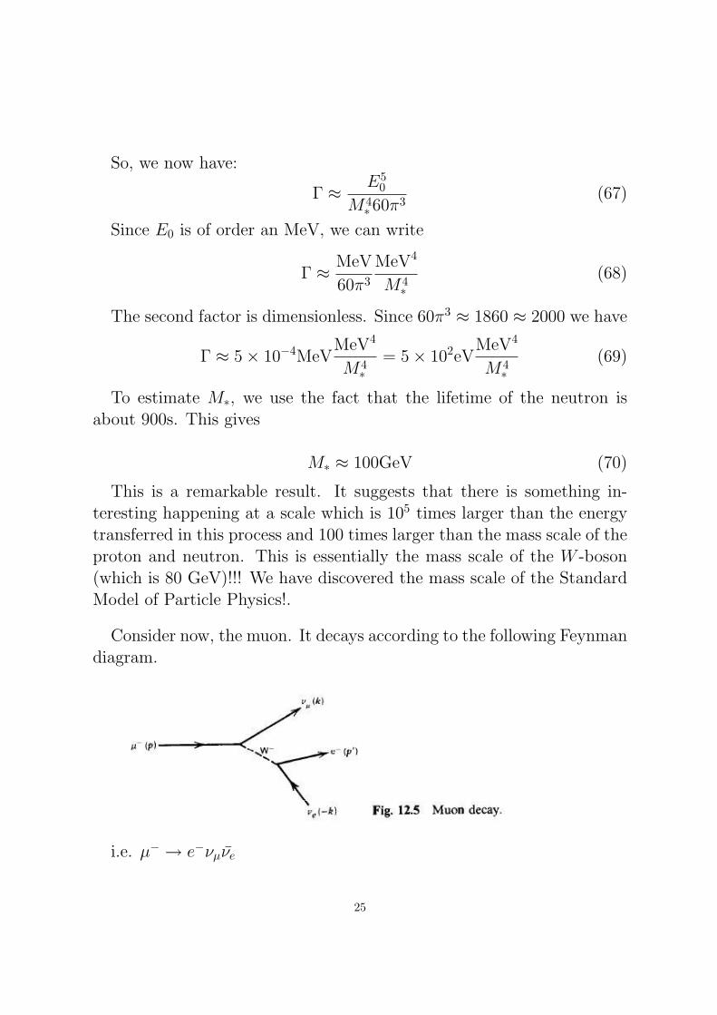
Consider now, the muon. It decays according to the following Feynmandiagram.
i.e. µ− → e−νµνe
25
Why does the muon decay? The answer is that there is nothing frompreventing this process to occur, so it will. The electron cannot decay, be-cause there is no combination of lighter particles with the correct chargesfor it to decay to. Hence, its mass and charge prevent it from decaying.The muon, on the other hand has the same charge as an electron, butweighs 200 times more.
What we see from the diagram is that, even though a W -boson weighs80 GeV, 800 times the muon mass, quantum mechanics allows this tooccur: the energy-time uncertainty relation,
∆E∆t ≥ 1
2(71)
allows a W -boson to be created for a very short amount of time. Notethat the W -boson which ”propagates” in the neutron and muon decaydiagrams is not on-shell i.e. it does not obey E2 = p2 + m2
W . It is theuncertainty relation that allows off-shell W ’s to propagate.
The diagram is completely analagous to the neutron decay diagram.In analogy with that one, we would estimate
Γ(µ− → e−νµνe) ≈m5µ
M 4∗60π3 (72)
M∗ ∼ MW . Hence we see that the presence of the W -boson in theintermediate state contributes a factor of 1/M2
W to the matrix element.This is the W -boson propagator for a process in which the energies aremuch smaller than MW . The actual propagator is proportional to 1
q2−M2W
c.f. the photon propagator.So, if we hadn’t done the calculation above we would have seen that
the decay width is proportional to 1M4W
and hence, dimensional analysis
would tell us that there is a m5µ present. The 60π3 would require knowing
that the final state ”phase-space” gives an additional suppression.The actual properly calculated muon decay width gives the result:
Γ(µ− → e−νµνe) ≈m5µ
M 4∗192π3 ≡ G2
F
m5µ
192π3 (73)
26

where GF is now defined to be equal to M−2∗ .
Use this to calculate the muon lifetime and compare it to the value inthe PDG (Particle Data book).
Calculate the lifetime of the τ -lepton.
1.4 Lorentz Invariant Phase Space Factor
Recall that the probability density, ρ = 2E|N |2. The integral of ρ in avolume V produces a factor of V , so we could choose the constant N suchthat this cancels, i.e.
N =1√V
(74)
and ∫V
d3xρ(E) = 2E (75)
This normalisation is thus one in which there are 2E particles in avolume V . Hence, with this normalisation, the number density becomes:
dn =V
2π3
d3p
2E(76)
note: if we had not chosen a value for N , we would still have the sameE dependence, but there would be a 1
N2 present as well. The final resultdoesn’t actually depend on N
The last expression for dn is Lorentz invariant! To see this, consider aLorentz boost in the z direction with velocity v:
E ′ = γ(E − vpz) (77)
p′z = γ(pz − vE) (78)
Then,dp′z = γdpz − γvdE (79)
sodp′zdpz
= γ(1− v)dE
dpz(80)
27

Now
dE
dpz=
d
dpz(p2x + p2
y + p2z +m2)1/2 = pz(p
2x + p2
y + p2z +m2)−1/2 =
pzE
(81)
Therefore:
dp′zdpz
= γ(1− vpzE
) (82)
= γ(E − vpz)
E(83)
= E ′/E (84)
Thereforedp′z/E
′ = dpz/E (85)
andd3p′
E ′=d3p
E(86)
28

1.5 Lifetime of a Particle
We now write the general formula for the differential decay width (itsdifferential because it is before we integrate over final state particles) ina relativistic, Lorentz invariant system.
Consider a particle A which decays into n particles. The transitionprobability (or differential decay width) is given by:
dΓ =1
2EA|M|2 d3p1
(2π)32E1....
d3pn(2π)32En
(2π)4δ4(pA−p1−p2− ...−pn) (87)
2EA is the number of decaying particles per unit volume, M the in-variant amplitude for the process. Note that there are no factors of thearbitrarily chosen normalisation volume V . Since dΓ is measurable, theresult should not depend on V (one can demonstrate this, but we willnot do this in class).
2 Cross-sections
In a particle collider experiment, we collide beams of particles with somegiven flux (also called luminosity and then we measure the particles thatcome out of the collisions. The total number of events is obviously pro-portional to the flux since e.g. if we increase the number of protons in theLHC beams we will increase the total number of collision events that weget. Thus, the luminosity is something that we control as experimentersin a laboratory. It is not an intrinsically physical entity.
However, the proportionality ”constant” in the relation
Nevents ∝ Luminosity ≡ L (88)
is an intrinsically physical quantity. This is called the cross-section andis usually labeled by σ.
Nevents = Lσ (89)
The left hand side is dimensionless, a whole number if we count thenumber of events (or collisions) after a given time interval. Or we could
29

consider the number of events per second (or any other unit of time). Theluminosity is thus a flux of particles per unit time. This has dimensionsof [L] = [L]−2[T ]−1 = [M ]3, where the last equality is because we usenatural units. The dimensions of luminosity are like this because it isessentially the number of particles going through a given area i.e. numberof particles per unit area per second.
So, by dimensional analysis, the cross-section σ has dimensions ofAREA. In fact, that is where its name comes from. It is, effectively,the area over which the interaction takes place.
2.1 Dimensional analysis calculations of σ
Lets get a feel for σ by estimating it for various processes. Our estimatesare based on Fermi’s Golden Rule plus dimensional analysis in naturalunits. We will also compare our results to the ”properly calculated”results as well as the actual experimental observations.
1. σ(e+e− → µ+µ−) at high energies.A Feynman diagram at leading order for this is the same as the in-
teraction between muons and electrons diagram above, but turned on itsside. We would like to estimate the cross-section for this at high centreof mass energies
√s much greater than mµ.
By now, we know that the answer for this will by proportional to the”square of the Feynman diagram” for this process. This tells us that:
σ ∝ e4 ∼ α2 (90)
because we have a factor of the charge at each vertex. α is dimensionless,a number with no units. But σ has dimension [M ]−2. The only otherscale in this problem is the center of mass energy
√s. Hence we expect
that
σ ∼ α2
s(91)
The actual ”properly calculated” leading order result is
30
σ =4π
3
α2
s(92)
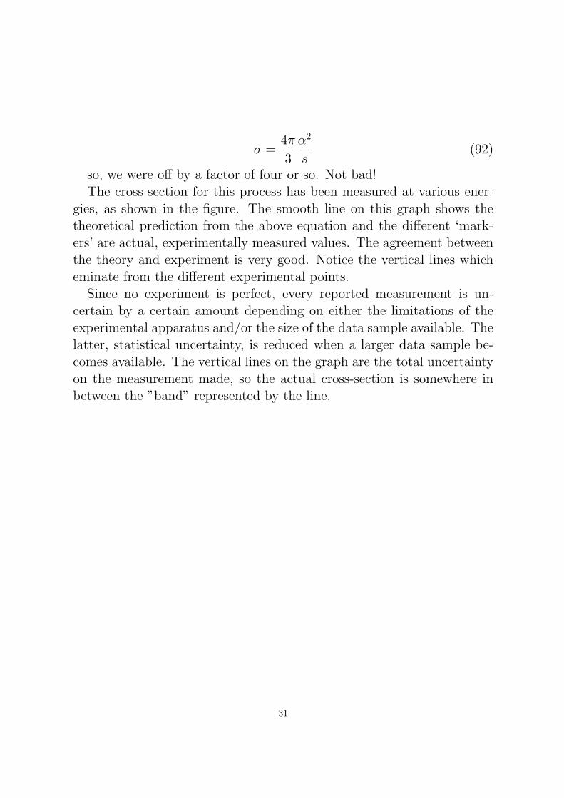
so, we were off by a factor of four or so. Not bad!The cross-section for this process has been measured at various ener-
gies, as shown in the figure. The smooth line on this graph shows thetheoretical prediction from the above equation and the different ‘mark-ers’ are actual, experimentally measured values. The agreement betweenthe theory and experiment is very good. Notice the vertical lines whicheminate from the different experimental points.
Since no experiment is perfect, every reported measurement is un-certain by a certain amount depending on either the limitations of theexperimental apparatus and/or the size of the data sample available. Thelatter, statistical uncertainty, is reduced when a larger data sample be-comes available. The vertical lines on the graph are the total uncertaintyon the measurement made, so the actual cross-section is somewhere inbetween the ”band” represented by the line.
31

Putting actual numbers to the cross-section we get:
σ(e+e− → µ+µ−) ∼ 4× 10⁻³²
s/GeV2 cm2 (93)
So in order to produce a few muon pairs in electron-positron scatteringat a centre-of-mass energy of one GeV, you need to have a luminosityof order 1032cm−2. At higher energies, since the cross-section decreasesquadratically with energy, you need much higher luminosities to producethe same number of muons.
2. σ(νN → X)Here we want to consider neutrinos interacting with nucleons in matter.
Neutrinos are not electrically charged so they don’t couple to photons.Nor do they participate in the strong nuclear interactions (like quarks andgluons do). But they do undergo weak interactions, eg via exchangingW -bosons and Z-bosons.
32

2.2 Centre-of-Mass Frame and Laboratory Frame
The centre of mass frame for a collision of two particles is one in whichthe two particles have equal and opposite momentum and equal energies.In this frame the Lorentz 4-vectors for the two particles are
pµ1 = (1/2Ecm, pi) (94)
pµ2 = (1/2Ecm,−pi) (95)
We can calculate the Lorentz invariant quantity s:
s = (p1 + p2)µ(p1 + p2)µ = E2
cm (96)
The laboratory frame is one in which one of the particles is at rest andthe other is moving.
pµ1 = (M, 0) (97)
pµ2 = (Elab, pilab) (98)
In the lab frame
s = (Elab +M)2 − E2lab +m2 ≈ 2ElabM (99)
where we assumed E to be much larger than M or m the two particlemasses.
Okay, back to neutrino cross-sectionSince neutrinos interact via the weak interaction, the |M|2 will be
proportional to G2F hence we will have that
σ(νN) ∼ G2F (100)
But σ must have mass dimension minus two. At high energies, theonly other scale in the problem is s which has mass dimension two.
Therefore, we expect that
σ(νN) ∼ G2Fs (101)
33

In most experimental situations with neutrinos we are normally in thelab frame, scattering a beam of neutrinos off a fixed target. e.g. thenucleons could be a ”block” of matter and the neutrino beam is ”fired”into it. Therefore s ∼ 2EνmN
Using the fact that mN ∼ 1 GeV and that GF ∼ 10−5 GeV−2 we get
σ(νN) ∼ afew × 10−38 Eν
GeVcm2 (102)
which is again in agreement with the ”proper calculation” to within afactor of 10.
Notice that this is a much smaller cross-section than the previous onewe estimated for a fixed centre-of-mass.
How far can neutrinos propagate through matter?
Imagine a neutrino which has been emitted by the sun (or any otherstar in the galaxy) and arrives at the Earth. We can use the resultabove to estimate how far a neutrino can propagate in the Earth beforeit actually interacts with a proton or neutron in the Earth.
Obviously the reaction rate is proportional to both the cross-section forthe reaction per nucleon (as estimated above) and the density of nucleonsi.e. the density of the Earth, ρ. The greater the reaction rate, the shorterthe distance a neutrino can propagate before interacting. Thus, we have,the average propagation distance L before an interaction takes place is:
L ∝ 1
ρσ(103)
where σ is calculated above for neutrinos interacting with nucleons andρ is the mass per unit volume of the matter through which the neutrinopropagates.
Now we use dimensional analysis. The length L has dimensions of[L] = [M ]−1. So, the RHS has to have the same dimensions. This willhelp us to fix the proportionality constant in the above. ρ has dimensionsof [M ]4 and [σ] = [M ]−2. Thus, if
34

L =C
ρσ(104)
the dimension of C is [C] = [M ]. Therefore we are looking for a quan-tity which plays an important role in the interaction between a neutrinoand a nucleon with the dimensions of mass. The obvious candidate is thenucleon mass, mN ∼ 1 GeV.
We therefore find:
L =mN
ρσ(105)
Notice that ρmN
is essentially the number of atoms per unit volume inthe Earth. Let us call this N . Hence we see that
L =1
Nσ(106)
If we take ρ ∼ 103kg/m3 ∼ 1030 GeV/m3. Since mN ∼GeV we havethat N ∼ 1030/m3. We have calculated σ above. For a neutrino withenergy of order 1 GeV
σ ∼ 10−38cm2 = 10−42m2 (107)
Hence, neutrinos with energies of order a GeV propagate roughly 1012m
through water before interacting! This is a billion kilometres. Most ofthe neutrinos from the sun have energies which are one hundred or moretimes less than a GeV and, hence they propagate much further.
3. σ(pp→ X)
The next cross-section we estimate is the cross-section for two hadrons(e.g. two protons) to interact. This is relevant for hadron colliders suchas the CERN LHC. This cross-section is different to those above becausehadrons are not point particles. Rather, they are bound states of quarks,anti-quarks and gluons, bound together by the strong nuclear force. Thestrong nuclear force is the SU(3) part of the Standard Model. The re-markable thing about the strong nuclear force is that all hadrons have
35

masses which are of order a GeV. In fact, most of the particles describedin the PDG are hadrons (either mesons or baryons). If you look at theirmasses, they are all within one order of magnitude of the proton mass.This reflects the fact that the strong nuclear force is characterised by ascale Λ ∼ GeV. This is known as the QCD scale since the underlying the-oretical description of the strong nuclear interaction is called QuantumChromodynamics.
Λ is essentially the binding energy of the quarks, anti-quarks and glu-ons inside any hadron. Since the u d and s quarks have masses whichare much smaller than Λ, the masses of hadrons made of these quarksare mostly binding energy. Therefore your mass, and the masses of allthe stars in the Universe is binding energy of the strong nuclear force.The b and c quarks have masses of order Λ itself, so c and b hadronshave masses which are not just binding energy. The t quark, which isthe most massive known elementary particle (mt ∼ 173GeV ± 1 GeV)actually decays before it has time to ”hadronise” and form a hadron.This is because τt = 1
Γt< 1
Λ .Exercise: Estimate the decay length of a b-hadron. Use the formula for
muon decay. Compare it to some of the b-hadron lifetimes in the PDG.
We want to calculate the cross-section for scattering two hadrons whichinteract via the strong nuclear interaction. We have just seen that ev-erything about the strong nuclear force is characterised by a single scaleΛ. Hence, we expect that the effective cross-section for strong nuclearinteractions is also determined by Λ. Hence,
σ(pp→ X) ∼ 1
Λ2 (108)
It is Λ−2 on dimensional grounds. This has the dimensions of a cross-section. Since GeV−1 ∼ 10−15m,
σ(pp→ X) ∼ 10−30m2 = 10−26cm2 (109)
Now, the in 2012, the LHC was running with an instantaneous lumi-nosity of about L = 1033cm−2s−1 at a centre of mass energy of 8 TeV.
36
Hence, with our rough estimate, we expect Lσ ∼ 107 events every second!Actually, our estimate is around a factor of 10 smaller than the actualanswer so we are producing even more collisions than that.
The greater the number of LHC collisions, the greater the probabilityof creating a ”rare” event such as the production of a Higgs boson. Thecross-section for producing a Higgs boson with a mass of around 126 GeVat the LHC is about 10−35cm2. This means that we have to ”sift through”around a billion events for every Higgs boson produced. The search forthe Higgs is thus very much like looking for a needle in a haystack.
Exercise: The Higgs boson mass is approximately 126GeV. How manyHiggs bosons were produced in the 2012 run of the LHC? For this youneed to find out how much data was recorded i.e. the total integratedluminosity.
3 Symmetries
3.1 Symmetries Commute with the Hamiltonian
Consider the Schrodinger equation
idΨ
dt= HΨ (110)
Suppose there is an Hermitian operator, K, with expectation value〈K〉.
Q: when is 〈K〉 conserved?By this we mean, when is 〈K〉 a constant of motion i.e.
d
dt〈K〉 = 0 (111)
This implies
0 =d
dt〈K〉 =
d
dt
∫Ψ∗KΨd3x (112)
Hence
37

∫dΨ
dt
∗KΨd3x+
∫Ψ∗K
dΨ
dtd3x = 0 (113)
Since
− idΨ
dt
∗= (HΨ)∗ = Ψ∗H (114)
we have that
−∫
Ψ∗HKΨd3x+
∫Ψ∗KHΨd3x = 0 (115)
Therefore:
KH −HK = 0 ≡ [K,H] (116)
i.e. the operator K commutes with the Hamiltonian.This implies that eigenstates of K are also eigenstates of H.
HΨ = EΨ (117)
KΨ = kΨ (118)
This implies that the states transformed into each other by K havethe same energy:
H(KΨ) = E(kΨ) (119)
ie Ψ and (KΨ) are degenerate in energy.
3.2 Lagrangians and Equations of Motion
In classical mechanics one considers generalised coordinates qi(t) of aparticle. Then the Lagrangian
L = T − V (120)
which is the difference between Kinetic and Potential energy leads tothe Euler-Lagrange equations of motion
38

d
dt
(dL
dqi
)− dL
dqi= 0 (121)
We can use this formalism to obtain the relativistic wave equationssuch as the Klein-Gordon equation, the Maxwell equations and the Diracequation.
Instead of considering L to be a function of discrete coordinates qi, weconsider Lagrangians which are functions of the fields which are contin-uous functions of both xi and t i.e. of xµ.
For example, for the Klein-Gordon equation L is a function of φ(xµ)as well as the derivatives ∂φ
∂xµ≡ ∂µφ:
L(qi, qi, t)→ L(φ, ∂µφ, xµ) (122)
L is obtained from a Lagrangian density L integrated over space
L =
∫d3xL(φ, ∂µφ) (123)
Integrating over time gives the action, usually called S:
S =
∫dtL =
∫d4xL (124)
By varying S wrt φ and ∂µφ and ∂µφ∗ we obtain the Euler-Lagrange
equations (this is derived at the end of the notes in the section onNoethers theorem):
∂µ
(δL
δ(∂µφ)
)− δLδφ
= 0 (125)
The Lagrangian density for the KG equation is
L = ∂µφ∗∂µφ−m2φ∗φ (126)
Substituting this into the Euler-Lagrange equations gives
∂µ∂µφ+m2φ = 0 (127)
39

Note: (δL
δ(∂µφ)
)= ∂µφ∗ (128)
The Lagrangian density for Maxwells equations in vacuum is
L = −1
4FµνF
µν (129)
Here we consider L as a function(al) of fields Aµ and derivatives ∂µAν.ie since Aµ has four components, we treat each component as a separatefield.
In the presence of a current jµ there is an additional interaction term
L = −1
4FµνF
µν − jµAµ (130)
3.3 Noether’s Theorem
Consider a small transformation in a field which leaves the Lagrangianinvariant
Ψ→ Ψ + iαΨ (131)
0 = δL =δLδΨ
δΨ +
(δL
δ(∂µΨ)
)δ(∂µΨ) + c.c. (132)
so
0 = iαΨδLδΨ
+ iα
(δL
δ(∂µΨ)
)(∂µΨ) + .. (133)
= iα
[δLδΨ− ∂µ
(δL
δ(∂µΨ)
)]Ψ + iα∂µ
(δL
δ(∂µΨ)Ψ
)+ ...
where, to get to the last line from the previous one we use that:
∂µ
(δL
δ(∂µΨ)Ψ
)=
(∂µ
δLδ(∂µΨ)
)Ψ +
(δL
δ(∂µΨ)
)∂µΨ (134)
40
Going back to the previous expression, the equation before the oneabove, there are several key points:
1. The last term is proportional to a total derivative. Hence, it onlycontributes to the action at the boundary of space-time ie at infinity. Re-quiring this term to vanish at infinity implies that: the action is extrem-ised (δS = 0) exactly when the Euler-Lagrange equations are satisfied(the term in square brackets) . We have thus derived the Euler-Lagrangeequations.
2. In the case that we require that Ψ → Ψ + iαΨ is a symmetryof the action, then, because the terms in square brackets vanish dueto the Euler-Lagrange equations, the total derivative term must vanisheverywhere not just at infinity. Hence,
3. When a variation of the fields is a SYMMETRY of the action, thereexists a conserved quantity:
4. This conserved quantity is a Lorentz 4-vector,(
δLδ(∂µΨ)Ψ
)which
obeys the equation
∂µ
(δL
δ(∂µΨ)Ψ
)= 0 (135)
5.(
δLδ(∂µΨ)Ψ
)is identified with the current jµ.
Any constant times jµ is also conserved and we put in the charge toidentify it with the current we discussed earlier in the course.
jµ =ie
2
(δL
δ(∂µΨ)Ψ
)(136)
Exercise: Verify that this gives the same expression as we had for thecurrent in the Klein-Gordon case.
The Lagrangian for Scalar QED ie a charged KG field
41

Recall (chapter 4 of book) that in order to consider the motion of aparticle of charge −e in an electromagnetic field generated by a vectorpotential Aµ we replace the derivative ∂µ by
∂µ → ∂µ − ieAµ (137)
We call the rhs of this expression a covariant derivative. This is usuallydenoted by Dµ:
Dµ ≡ ∂µ − ieAµ (138)
Recall that, by making the above replacement in the Klein-Gordonequation we obtained
∂µ∂µφ+m2φ = −V φ (139)
where
V = −ie(∂µAµ − Aµ∂µ)− e2AµAµ (140)
i.e. we get a potential V for the field φ. Since the modified equationof motion was obtained by replacing ∂µ with Dµ, the Lagrangian densityfor a charged scalar is
L = Dµφ(Dµφ)∗ −m2φφ∗ (141)
= ∂µφ∂µφ∗ − ieAµφ∂
µφ∗ + ie∂µφAµφ∗ − e2AµA
µφφ∗ −m2φφ∗
Notice that the second and third terms in the last expression combineto give
L = ∂µφ∂µφ∗ − jµAµ − e2AµA
µφφ∗ −m2φφ∗ (142)
ie we have written them in terms of the conserved current. Thus,combining this Lagrangian with that of Maxwell’s theory we have thefull Lagrangian for scalar QED:
L = −1
4FµνF
µν +Dµφ(Dµφ)∗ −m2φφ∗ (143)
42

Feynman Diagrams and the Lagrangian
When we studied scalar QED before introducing it in Lagrangian form,we saw that jµAµ appears in the invariant amplitude M for a process.
The fact that jµAµ appears in L suggests that we can just ”read off”the vertices allowed in Feynman diagrams from L. This is a general rulefor any Lagrangian! We just read off the Feynman rules from L .
In this example, the three point vertex between the photon and twocharged particles is represented in L by the presence of the jµAµ term.
Symmetries of Scalar QED
The Lagrangian for scalar QED has various symmetries.Lorentz Invariance. Since all the Lorentz indices are contracted (L is
a scalar), the Lagrangian is invariant under Lorentz transformations.Internal Symmetry. In addition to this ”spacetime symmetry” it is
invariant under an internal symmetry i.e. one which does not act on thecoordinates, but just on the fields. This is intrinsic to electromagnetismand the other forces as we will see.
Gauge Symmetry
43

We are going to consider a transformation of φ by a unitary, 1-by-1matrix, a U(1) transformation.
Any such matrix U is of the form U(α) = eiα. α can take any contin-uous value between zero and 2π.
Clearly, underφ→ Uφ (144)
we have thatDµφ→ UDµφ (145)
TheDµφ(Dµφ)∗ term is clearly invariant under this transfomation sinceit is of the form Dµφ times its complex conjugate, and UU ∗ = 1. Similarlyφφ∗ is invariant, so the mass term is invariant. Therefore L is invariantunder this transformation of φ.
Noethers theorem proves that there is a conserved quantity when aLagrangian is invariant under a symmetry transformation. In fact, whenα is small i.e. when U ≈ 1 + iα we see that the conserved current jµ isprecisely that which we derived before.
Now, we would like to consider the case that α is different from pointto point in spacetime. i.e. we make α = α(xν) – a function of thecoordinates. Clearly this will change the above conclusions because wewill get terms proportional to derivatives of α.
Dµφ → U∂µφ+ iU∂µαφ− ieUAµφ (146)
= UDµφ+ iU∂µαφ (147)
Thus, because of the term proportional to the derivative of α the La-grangian is no longer invariant.
However, the unwanted term in the transformation of Dµφ can beremoved if Aµ also transforms:
Aµ → Aµ +1
e∂µα (148)
which can be verified by replacing this transformed Aµ in the ”un-wanted” term.
44

Therefore, we have that
Dµφ→ eiα(x)Dµφ (149)
and the Klein-Gordon terms in the Lagrangian are invariant underthis gauge transformation (this is the name for transformations whoseparameters are functions of the coordinates.
What about the Maxwell term in the Lagrangian?Let us consider the electromagnetic field strength, Fµν.Since
Fµν = ∂µAν − ∂νAµ (150)
the field strength transforms into
Fµν → ∂µAν −1
e∂µ∂να− ∂νAµ +
1
e∂ν∂µα (151)
= ∂µAν − ∂νAµ = Fµν (152)
Therefore Maxwell’s Lagrangian also gauge invariant!
Gauge Symmetry as a Principle
If we use gauge symmetry as a principle then it has far reaching con-sequences.
1. The covariant derivative must be introduced otherwise the kineticenergy term would not be gauge invariant.
2. This requires the introduction of a vector field Aµ which couples tothe matter current. Aµ is usually called the gauge field.
3. If we consider the kinetic energy of the gauge field, then gaugeinvariance requires it to be of the form FµνF
µν (or more generally a func-tion thereof). Thus, Maxwell’s equations follow from gauge symmetryplus Lorentz symmetry
4. The photon is massless
45

This last point is crucial. It provides an explanation for why the photonessentially behaves as a massless particle. (Experimentally of course onecannot prove that the photon is exactly massless. Rather, one obtainsan upper limit on its mass. The current upper limit is about 10−18 eV.)
To see why the photon is massless, we ask: what would a mass termlook like?. Well, in analogy with the mass term of the KG equation itwould be of the form:
∂ν∂νAµ +m2Aµ = 0 (153)
This mass term would arise from a term in the Lagrangian of the form
∆L ∼ −m2AµAµ (154)
Such a term is clearly not invariant under the gauge transformation ofAµ, which is
Aµ → Aµ +1
e∂µα (155)
In fact, combining all of these points, the most general gauge andLorentz invariant Lagrangian which is quadratic in the fields and theirderivatives is
L = −1
4FµνF
µν +Dµφ(Dµφ)∗ −m2φφ∗ (156)
Thus: the symmetries determine the Lagrangian and, hence, the physics
This is a key point in particle physics. The Lagrangian for the Stan-dard Model is essentially determined by its symmetries. In other words,symmetries determine the physics of all elementary particles!
46

Beyond U(1) Gauge Invariance
We would now like to consider generalising U(1) gauge theory (i.e.QED) to U(N) gauge theory.
That is to say that U – the transformation matrix – will become aUnitary N ×N matrix U i
j where i, j run from 1 to N each.An N × N matrix acts naturally on N component vectors vi. Hence
we should introduce N complex scalar fields φi on which these act.Under
φi → U jiφj (157)
we would like to impose a condition that a suitable covariant derivativetransforms acting on φi transforms in the same way
(Dµφ)i → U ji (Dµφ)j (158)
This would be the N ×N generalisation of the U(1) case.But what is this covariant derivative?If we try to introduce a gauge field, in general it is a matrix of gauge
fields i.e. we can have up to N ×N gauge fields:
(Dµφ)i = ∂µφi − ig(Gµ)jiφj (159)
that is, for each of the values of i and j, (Gµ)ij is a different gauge field.
47

Unitary matrices, exponentials, group generators and all thatIn order to understand a little better the structure we would like to
look at some of the simple symmetry groups like SU(2) and SU(3). First,though we begin with U(1):
exp iθ = 1 + iθ − θ2
2− iθ
3
3!+θ4
4!+ ..... = cos θ + isin θ (160)
Now consider the rotation matrix
R(θ) ≡(
cos θ sin θ−sin θ cos θ
)(161)
We want to Taylor expand this matrix
(cos θ sin θ−sin θ cos θ
)=
(1− θ2
2 + θ4
4! + ... θ − θ3
3! + ...
−θ + θ3
3! + ... 1− θ2
2 + θ4
4! + ...
)(162)
Just as eiθ is the exponential of a 1-by-1 matrix, the rotation matrixabove is the exponential of a two-by-two matrix:
R(θ) = exp(iθT ) = 1 + iθT − θ2
2T 2 − iθ
3
3!T 3 + ... (163)
where
T =
(0 −ii 0
)(164)
and T 2 is the matrix product of T with itself.So, since any rotation can be written as exp iθT we say that T generates
the rotations.Let us now consider some other examples of this, because we will need
matrices like T to define the covariant derivative properly.Let U be a N-by-N unitary matrix ie
U †.U = 1 (165)
48

We will now assume that
U = exp iM (166)
What properties does M have?Since
U † = exp(−iM †) (167)
unitarity implies thatM = M † (168)
So, M is Hermitian.If, additionally, we require that det(U) = 1 i.e. that U is special
unitary, then one can show that the trace of M is zero
detU = 1↔ TrM = 0 (169)
SU(2)
For the case N = 2, one can show that M is a linear combination ofthe Pauli matrices:
M = αaσa (170)
where
σ1 =
(0 11 0
)(171)
σ2 =
(0 −ii 0
)(172)
σ3 =
(1 00 −1
)(173)
That is to say that the Pauli matrices generate SU(2) transformationmatrices!
An important fact about the Pauli matrices is that they obey an alge-bra:
[σa, σb] = 2iεabcσc (174)
49

A note on εabcεabc is the same as εab
c – we put the third index up to remind us that weare summing over c. εabc is totally antisymmetric i.e. if we interchangeneighbouring indices then we get a minus sign:
εabc = −εbac = εbca = −εcba etc (175)
This implies that all three indices of εabc must take different values inorder to get a non-zero result otherwise it would not be totally antisym-metric.
Therefore εabc is non-zero if and only if (abc) is a permutation of (123).Finally,
ε123 = 1 (176)
For all of the other five permutations of (123) the value of εabc can beobtained from antisymmetry. Thus, for example ε132 = −1.
Back to SU(N).
In general, for an SU(N) matrix
U = exp iM (177)
where M is traceless and Hermitian, there are N 2 − 1 generators Tasuch that
M = αaTa (178)
and the Ta ’s obey an algebra
[Ta, Tb] = ifabcTc (179)
where the fabc are constants called the structure constants. For SU(N)
the algebra defined by the above equation is called the Lie Algebra ofSU(N). If you choose a basis for this algebra, you can explicitly calculatethe structure constants in that basis. They are totally antisymmetric, likeεabc. For SU(3) there is a basis for the eight 3-by-3 Ta matrices which isused a lot in particle physics called the Gell-Mann basis. You can findthese eight matrices in the book.
50

Finally
Dµ = ∂µ + igTaGaµ (180)
where the second term is an N -by-N matrix since Ta is a matrix.There are N 2 − 1 gauge fields Ga
µ.
The Standard Model is a gauge theory with SU(3) gauge symmetry,SU(2) gauge symmetry and U(1) gauge symmetry. There are 8+3+1 =12 gauge bosons. These are the eight gluons, the two W -bosons (W+ andW−), the neutral Z boson and the photon.
The full covariant derivative is thus
Dµ = ∂µ − iY
2g1Bµ − ig2
σj2W j
µ − ig3λa2Gaµ (181)
Bµ is the gauge boson of the U(1). The photon is a linear combinationof Bµ and W 3
µ . The Z-boson is the opposite linear combination.Y is called the hypercharge. The charge under SU(2) is called isospin
I. The proton has isospin 1/2 and the neutron −1/2.The proton and neutron transform as a doublet under the SU(2) of
the Standard Model: (p
n
)→ exp(iM)
(p
n
)(182)
Electric charge is a linear combination of Y and I.
Q = I + Y/2 (183)
Both p and n have to have the same Y which is one.Similarly, in the Standard Model u and d quarks transform under
SU(2) (ud
)→ exp(iM)
(ud
)(184)
Note: this is not strictly speaking correct: fermions can be left-handedor right-handed as we will see when we study the Dirac equation. This is
51

related to the fact they are not scalars, but fermions i.e. it is related totheir spin under rotations. The correct statement is that the left-handedup and down quarks transform under SU(2) as above. In fact, righthanded fermions do NOT transform atall under the SU(2) i.e. for themI=0. Thus, when the covariant derivative acts on right-handed fermions,the term proportional to the Bµ boson is zero.
Hence left-handed u-quarks have I = 1/2, Y = 1/6 whereas right-handed u-quarks have I = 0, Y = 4/3. Both of these charges giveQ = 2/3. Similarly, e−L the left-handed electron has I = −1/2, Y = −1whereas e−R has Y = −2. Left-handed electron-neutrinos are SU(2) part-ners of left-handed electrons, hence they have I = 1/2, Y = −1.
No right-handed neutrinos have been directly observed to exist (yet).The reason is the following. If they did exist, they would not transformunder SU(2) like all of the other right-handed neutrinos, hence have bothI = 0 and Y = 0. Therefore, such neutrinos would not couple to Bµ orthe SU(2) gauge fields W i
µ. Since neutrinos do not participate in thestrong interactions, the SU(3) part of the covariant derivative would alsonot act on the right-handed neutrino field. Therefore, the right-handedneutrino does not feel any force directly: its equation of motion does notinclude a gauge field. Such neutrinos are also called sterile neutrinos,for reasons which should hopefully be clear. Since they do not couple togauge bosons it is very difficult to produce or detect them in a laboratory.
Beyond U(1) Gauge Invariance
We would now like to consider generalising U(1) gauge theory (i.e.QED) to U(N) gauge theory.
That is to say that U – the transformation matrix – will become aUnitary N ×N matrix U i
j where i, j run from 1 to N each.An N × N matrix acts naturally on N component vectors vi. Hence
we should introduce N complex scalar fields φi on which these act.Under
φi → U jiφj (185)
52

we would like to impose a condition that a suitable covariant derivativetransforms acting on φi transforms in the same way
(Dµφ)i → U ji (Dµφ)j (186)
This would be the N ×N generalisation of the U(1) case.But what is this covariant derivative?If we try to introduce a gauge field, in general it is a matrix of gauge
fields i.e. we can have up to N ×N gauge fields:
(Dµφ)i = ∂µφi − ig(Gµ)jiφj (187)
that is, for each of the values of i and j, (Gµ)ij is a different gauge field.
53

Unitary matrices, exponentials, group generators and all thatIn order to understand a little better the structure we would like to
look at some of the simple symmetry groups like SU(2) and SU(3). First,though we begin with U(1):
exp iθ = 1 + iθ − θ2
2− iθ
3
3!+θ4
4!+ ..... = cos θ + isin θ (188)
Now consider the rotation matrix
R(θ) ≡(
cos θ sin θ−sin θ cos θ
)(189)
We want to Taylor expand this matrix
(cos θ sin θ−sin θ cos θ
)=
(1− θ2
2 + θ4
4! + ... θ − θ3
3! + ...
−θ + θ3
3! + ... 1− θ2
2 + θ4
4! + ...
)(190)
Just as eiθ is the exponential of a 1-by-1 matrix, the rotation matrixabove is the exponential of a two-by-two matrix:
R(θ) = exp(iθT ) = 1 + iθT − θ2
2T 2 − iθ
3
3!T 3 + ... (191)
where
T =
(0 −ii 0
)(192)
and T 2 is the matrix product of T with itself.So, since any rotation can be written as exp iθT we say that T generates
the rotations.Let us now consider some other examples of this, because we will need
matrices like T to define the covariant derivative properly.Let U be a N-by-N unitary matrix ie
U †.U = 1 (193)
54

We will now assume that
U = exp iM (194)
What properties does M have?Since
U † = exp(−iM †) (195)
unitarity implies thatM = M † (196)
So, M is Hermitian.If, additionally, we require that det(U) = 1 i.e. that U is special
unitary, then one can show that the trace of M is zero
detU = 1↔ TrM = 0 (197)
SU(2)
For the case N = 2, one can show that M is a linear combination ofthe Pauli matrices:
M = αaσa (198)
where
σ1 =
(0 11 0
)(199)
σ2 =
(0 −ii 0
)(200)
σ3 =
(1 00 −1
)(201)
That is to say that the Pauli matrices generate SU(2) transformationmatrices!
An important fact about the Pauli matrices is that they obey an alge-bra:
[σa, σb] = 2iεabcσc (202)
55

A note on εabc
εabc is the same as εabc – we put the third index up to remind us that we
are summing over c. εabc is totally antisymmetric i.e. if we interchangeneighbouring indices then we get a minus sign:
εabc = −εbac = εbca = −εcba etc (203)
This implies that all three indices of εabc must take different values inorder to get a non-zero result otherwise it would not be totally antisym-metric.
Therefore εabc is non-zero if and only if (abc) is a permutation of (123).Finally,
ε123 = 1 (204)
For all of the other five permutations of (123) the value of εabc can beobtained from antisymmetry. Thus, for example ε132 = −1.
Back to SU(N).
In general, for an SU(N) matrix
U = exp iM (205)
where M is traceless and Hermitian, there are N 2 − 1 generators Tasuch that
M = αaTa (206)
and the Ta ’s obey an algebra
[Ta, Tb] = ifabcTc (207)
where the fabc are constants called the structure constants. For SU(N)
the algebra defined by the above equation is called the Lie Algebra ofSU(N). If you choose a basis for this algebra, you can explicitly calculatethe structure constants in that basis. They are totally antisymmetric, likeεabc. For SU(3) there is a basis for the eight 3-by-3 Ta matrices which isused a lot in particle physics called the Gell-Mann basis. You can findthese eight matrices in the book.
56

Finally
Dµ = ∂µ + igTaGaµ (208)
where the second term is an N -by-N matrix since Ta is a matrix.There are N 2 − 1 gauge fields Ga
µ.
The Standard Model is a gauge theory with SU(3) gauge symmetry,SU(2) gauge symmetry and U(1) gauge symmetry. There are 8+3+1 =12 gauge bosons. These are the eight gluons, the two W -bosons (W+ andW−), the neutral Z boson and the photon.
The full covariant derivative is thus
Dµ = ∂µ − iY
2g1Bµ − ig2
σj2W j
µ − ig3λa2Gaµ (209)
Bµ is the gauge boson of the U(1). The photon is a linear combinationof Bµ and W 3
µ . The Z-boson is the opposite linear combination.Y is called the hypercharge. The charge under SU(2) is called isospin
I. The proton has isospin 1/2 and the neutron −1/2.The proton and neutron transform as a doublet under the SU(2) of
the Standard Model: (p
n
)→ exp(iM)
(p
n
)(210)
Electric charge is a linear combination of Y and I.
Q = I + Y/2 (211)
Both p and n have to have the same Y which is one.Similarly, in the Standard Model u and d quarks transform under
SU(2) (ud
)→ exp(iM)
(ud
)(212)
Note: this is not strictly speaking correct: fermions can be left-handedor right-handed as we will see when we study the Dirac equation. This is
57

related to the fact they are not scalars, but fermions i.e. it is related totheir spin under rotations. The correct statement is that the left-handedup and down quarks transform under SU(2) as above. In fact, righthanded fermions do NOT transform atall under the SU(2) i.e. for themI=0. Thus, when the covariant derivative acts on right-handed fermions,the terms proportional to the Wµ bosons is zero.
Hence left-handed u-quarks have I = 1/2, Y = 1/6 whereas right-handed u-quarks have I = 0, Y = 4/3. Both of these charges giveQ = 2/3. Similarly, e−L the left-handed electron has I = −1/2, Y = −1whereas e−R has Y = −2. Left-handed electron-neutrinos are SU(2) part-ners of left-handed electrons, hence they have I = 1/2, Y = −1.
No right-handed neutrinos have been directly observed to exist (yet).The reason is the following. If they did exist, they would not transformunder SU(2) like all of the other right-handed neutrinos, hence have bothI = 0 and Y = 0. Therefore, such neutrinos would not couple to Bµ orthe SU(2) gauge fields W i
µ. Since neutrinos do not participate in thestrong interactions, the SU(3) part of the covariant derivative would alsonot act on the right-handed neutrino field. Therefore, the right-handedneutrino does not feel any force directly: its equation of motion does notinclude a gauge field. Such neutrinos are also called sterile neutrinos,for reasons which should hopefully be clear. Since they do not couple togauge bosons it is very difficult to produce or detect them in a laboratory.
58

Spin, Fermions and the Dirac Equation
Spin
In quantum mechanics, particles have an intrinsic spin under spatialrotations of space. This is analagous to the rotation of ”classical objects”such as planets or spiniing tops, but the spin of elementary particlesis quantised (comes in discrete amounts). In natural units the allowedspins are half-integer or integer. Bosons have integer spins; fermionshalf-integer spins.
The Algebra of Rotations
We saw in the last lecture that rotations in a plane by an angle θ aregenerated by a matrix:
R(θ) = exp(iθT ) = 1 + iθT − θ2
2T 2 − iθ
3
3!T 3 + ... (213)
where
T =
(0 −ii 0
)(214)
We can use this observation to generate all rotations in three dimen-sional space. These are given by 3-by-3 matrices. Rotations in the (x, y)plane around the z-axis are of the form
Rz(θz) =
cos θz sin θz 0−sin θz cos θz 0
0 0 1
(215)
Show that these are generated by
T3 ≡
0 −i 0i 0 00 0 0
(216)
Similarly, a rotation around the x-axis
Rx(θx) =
1 0 00 cos θx sin θx0 −sin θx cos θx
(217)
59

is generated by
T1 ≡
0 0 00 0 −i0 i 0
(218)
and rotations around the y-axis
Ry(θy) =
cos θy 0 sin θy0 1 0
−sin θy 0 cos θy
(219)
are generated by
T2 ≡
0 0 −i0 0 0i 0 0
(220)
Thus, any rotation in three dimensional space can be generated by alinear combination of T1, T2, T3. The generators Ta obey an algebra:
[Ta, Tb] = iεabcTc (221)
We have seen this algebra before. The Pauli matrices satisfy
[σa, σb] = 2iεabcσc (222)
Hence,
[1
2σa,
1
2σb] = iεab
c1
2σc (223)
Therefore the Ta and 12σa obey precisely the same algebra, even though
the T ’s are 3-by-3 matrices and the Pauli matrices are 2-by-2.
We have shown that the algebra of rotations is the same as that of SU(2)
Every 3-by-3 rotation matrix can be specified by choosing (θx, θy, θz).From these we can specify a 2-by-2 SU(2) matrix. This gives a corre-spondence between rotations and elements of SU(2). For example, Rx(θx)corresponds to the matrix
Mx(θx) = exp
(iθx2σ1
)(224)
60

The 3-by-3 rotation matrices act on 3-component vectors, such as thespatial coordinates or the momentum of a particle. 3-by-3 rotations obey
R(θx, θy, θz) = R((θx + 2π, θy, θz) = R(θx, θy + 2π, θz) = R(θx, θy, θz + 2π)(225)
So a vector returns to itself after a full 2π rotation.However,
Mx(θx + 2π) = −Mx(θx) (226)
Mathematically, 2-component objects which transform under spatialrotations via SU(2) matrices are called spinors. Fermion wave functionsare represented by spinors. Fermions are said to have spin ”one-half”:they come back to themselves after two 2π rotations in space. In fact, inthe Pauli basis, the entries of 1
2σ3 give the spin of the two components ofthe fermion wave function, which are ±1
2 .
Spins are Classified
A set of three N -by-N matrices which obey the algebra:
[Wa,Wb] = iεabcWc (227)
is called a representation of the Lie algebra of SU(2) (or the algebraof rotations) with dimension N . The Pauli matrices are a 2-dimensionalrepresentation, the T ’s a 3-dimensional one.
All possible sets of matrices obeying the algebra can be completelyclassified. In fact, there are representations for any integer N . The Ncomponents of the vector on which the W ’s act have spins which are(N/2−1/2, N/2−3/2, N/2−5/2....,−N/2+1/2) . The highest spin of arepresentation i.e. N/2− 1/2 is also used to label the representation andis usually called the ”spin of the representation”. Any positive integer orhalf-integer is the highest spin of a set of W ’s obeying the algebra above.
So, representations with oddN have spins which are all integers. Thosewith N even, have all the spins strictly taking half-integer values. Theodd N representations are said to be bosonic whilst the half-integer spinrepresentations are called fermionic.
61
Scalar fields transform in the spin zero representation, N = 1. Quarksand Leptons in the spin 1/2 representation, N = 2 and gauge fields, beingvector fields, transform in the spin 1 representation, N = 3
Notice that in the 2-by-2 representation given by the Pauli matrices,one of the generators (1
2σ3) is diagonal. It’s eigenvalues are the spins of therepresentation, in this case 1
2 and −12 . In the 3-by-3 representation given
above, all three generators are off-diagonal, however their eigenvalues are(1, 0,−1) so the spins of the 3-dimensional representation are 1,0 and -1.
Since the rotations are part of the Lorentz symmetry, spin is conservedin physical processes.
So, when a W -boson of spin one decays into two particles A and B,the only possibilities are that A and B have spins 0 and 1, 1 and 0, or1/2 and 1/2. In the Standard Model, only the last possibility is realisedbecause in order to realise the first two, the spin 0 particle would haveto be the Higgs (the only scalar field present) and the spin 1 particlewould have to have be charged because charge is also conserved. Theonly charged spin 1 particles in the Standard Model are the W -bosons,which obviously, cannot decay into themselves.
The Dirac Equation
Dirac wanted to write a wave equation consistent with Lorentz invari-ance that was linear in the time derivative as in the Schrodinger equation.He wanted to do this to remove the negative energy solutions of the Klein-Gordon equation. He succeeded in finding a Lorentz covariant equationlinear in ∂
∂t but the negative energy solutions still remained. We knownow (as we discussed) that the negative energy solutions are associatedwith anti-particles. The Dirac equation describes relativistic fermions.We will derive the Dirac equation for free fermions, then, after exploringit’s properties we will write the Dirac equation for fermions interactingwith gauge fields. Then we will explore the interactions between fermionsand gauge fields and explore some of the consequences.
The starting point of Dirac’s argument was the hypothesis that the
62
equation should be of the form:
HΨ = (αipi + βm)Ψ (228)
where the left hand side is, as usual, linear in ∂∂t . αi and β are coeffi-
cients to be determined.The term proportional to mass must be present, since a particle with
mass m has energy m when its momentum is zero. The term proportionalto the momentum must be present since we are looking for an equationwhich treats space and time (and hence momentum and energy) on anequal footing. We determine the coefficients by demanding that, for afree particle solution
H2Ψ = (pipi +m2)Ψ (229)
From the first equation we have that
H2Ψ = (αipi + βm)(αjpj + βm)Ψ (230)
= (α2i p
2i + (αiαj + αjαi)pipj + (αiβ + βαi)pim+ β2m)Ψ
Where the first term on the rhs of the second line are the three termsin the product when i = j, the second and third terms are the remainingsix possibilities when i 6= j.
So, we learn that
• α1, α2, α3 and β all anti-commute with each other.
• α21 = α2
2 = α23 = β2 = 1
So, the coefficients cannot be numbers. Dirac realised that if they werematrices then solutions to these conditions indeed exist. With m 6= 0, (itcan be shown, but we won’t do so) the simplest solution has the αi andβ 4-by-4 matrices. Thus, Ψ is now understood to be a vector with fourcomponents i.e.
Ψ ≡ ΨA =
Ψ1
Ψ2
Ψ3
Ψ4
(231)
63

Ψ is called a Dirac spinor. There are actually different solutions forthe matrices, though physical results don’t depend on this choice.
One representation for the (αi, β) is called the Dirac-Pauli representa-tion and is given by
αi =
(0 σiσi 0
)β =
(I 00 − I
)(232)
where I is the 2-by-2 identity matrix.Another useful representation is the Weyl representation:
αi =
(−σi 00 σi
)β =
(0 II 0
)(233)
Covariant Form of the Dirac Equation
We can multiply the original form of the Dirac equation on the left byβ to obtain
iβ∂
∂tΨ = −iβαi
∂
∂xiΨ +mΨ (234)
which can be written as
(iγµ∂µ −m)Ψ = 0 (235)
where we have introduced the so-called Dirac γ-matrices
γµ ≡ (β, βαi) (236)
and we have anticipated the fact that the four γ-matrices transformunder Lorentz transformations as a Lorentz 4-vector.
In the above form we have suppressed the spinor matrix labels on γµ
and the spinor labels on Ψ. If we put these back in we have:
4∑K=1
[∑µ
i(γµ)JK∂µ −mδJK
]ΨK = 0 (237)
64

The original relations on the αi and β required by relativistic invarianceare equivalent to
γµγν + γνγµ = 2gµν (238)
where gµν is the Minkowski metric.
CurrentsWe now proceed as we did with the KG equation to obtain a form of
the current.For this we need the Hermitian conjugate of the Dirac equation:
− i∂Ψ†
∂tγ0 − i∂Ψ†
∂xk(−γk)−mΨ† = 0 (239)
This does not look terribly covariant since, whilst γ0 is Hermitian, theγk are anti-Hermitian. However, by defining
Ψ ≡ Ψ†γ0 (240)
we see that
i∂µΨγµ +mΨ = 0 (241)
We now multiply the Dirac equation on the left by Ψ, the conjugateequation above by Ψ and add the two. The mass terms cancel and wesee that
Ψγµ∂µΨ + (∂µΨ)γµΨ = ∂µ(ΨγµΨ) = 0 (242)
so that ΨγµΨ is conserved.Putting in the required factor of the charge, we then will have, for a
fermion of charge −e the charge current density is
jµ = −eΨγµΨ (243)
Solutions of the Dirac Equation
65

We now turn to solutions of the Dirac equation. It is convenient tointroduce the Feynman ”slash” notation which is defined as /V ≡ γµVµfor any four-vector Vµ.
Thus, the Dirac equation can be written as
(i/∂ −m)Ψ = 0 (244)
Since (see exercise sheets) the Dirac equation implies the KG equation,we have
(∂µ∂µ +m2)ΨA = (� +m2)ΨA = 0 (245)
and we can write
Ψ = u(pµ)e−ipµxµ (246)
where the 4-particle spinor u(p) is independent of x and satisfied themomentum space Dirac equation
(/p−m)u = 0 (247)
The Hamiltonian H is obtained from Diracs original ansatz
Hu = (αipi + βm)u = Eu (248)
There are actually four independent solutions of this equation. Twohave E > 0 and two have E < 0. To see this, consider fermions at restpi = 0. Let us use the Dirac-Pauli rep for the γ-matrices. Then
Hu = βmu =
m 0 0 00 m 0 00 0 −m 00 0 0 −m
u1
u2
u3
u4
which obviously has two positive and two negative eigenvalues. The
two positive energy solutions are interpreted as describing an E > 0electron, the two E < 0 solutions are interpreted as describing an E > 0positron.
66

For non-zero momentum, the equation becomes
Hu =
(m σip
i
σipi −m
)(uAuB
)= E
(uAuB
)(249)
where
u ≡(uAuB
)(250)
we therefore have that
σipiuB = (E −m)uA (251)
σipiuA = (E +m)uB (252)
(253)
To solve the equations we pick the two positive energy solutions u1 andu2 to have
u1A =
(10
), u2
A =
(01
)(254)
Then the remaining components of u1 and u2, namely u1B and u2
B aredetermined as
usB =σip
i
E +musA (255)
So, u1 and u2, the positive energy solutions of the Dirac equation aregiven by
us = N
(usA
σipi
E+musA
)(256)
Similarly, to obtain the two negative energy solutions u3 and u4 wetake the lower components (uB) of the Dirac spinor to be
u3B =
(10
), u4
B =
(01
)(257)
This gives the negative energy solutions as
us+2 = N
(−σipiE−mu
sA
usA
)(258)
67

Helicity
Consider the following 4-by-4 matrix:
Λ ≡ 1
2
(σip
i 00 σip
i
)(259)
where pi = pi
|p| satisfies pipi = 1 i.e. is the unit vector which points in
the same direction as pi. Λ commutes with the Hamiltonian. Therefore,the eigenvalues of Λ are conserved.
12σip
i is clearly the spin projected in the direction of motion. We callthis the helicity of the state. The possible eigenvalues of 1
2σipi are just
λ = ±12 .
We say that fermions with helicity −1/2 are left-handed and thosewith helicity 1/2 are right-handed.
Massless Dirac Equation and Helicity
The Dirac spinor has four components, whereas by considerations ofspin we expected two. The four are divided into two sets of two: left-handed and right-handed. Thus the Dirac spinor for a fermion describesboth the left- and right-handed helicity states. We can see this a bitmore clearly by considering the Dirac equation for m = 0 i.e. masslessfermions. Then β drops out and the αi have to satisfy
αiαj + αjαi = 2δij , α†i = αi (260)
These conditions can be solved by 2-by-2 matrices, αi = σi. Thus theDirac equation in the massless case can be satisfied by a 2-componentspinor, φ and we have:
Hφ = σipiφ (261)
In this case, E2 = pipi so, |E| = |p|. Hence we have
± |p|φ = σipiφ (262)
Consider now the positive energy solution E = |p|, φ+. It has
σipiφ+ = φ+ (263)
68

Therefore φ+ is right-handed in this case. The second solution φ− hasnegative energy E = −|p|, so in this case
σipiφ− = −φ− (264)
When the energy is −E and the momentum −pi, we have
σi(−pi)φ− = −φ− (265)
and describes a left-handed anti-fermion. So, if we apply this to a neu-trino in situations where |E| >> m, φ describes a right-handed neutrinoνR and a left-handed anti-neutrino νL.
We could have also chosen αi = −σi. In this case we would have
Eχ = −σipiχ (266)
The two solutions χ± describe a left-handed neutrino νL and a right-handed anti-neutrino νR. Only left-handed neutrinos and right-handedanti-neutrinos have been observed in nature.
We can combine χ and φ into a four component Dirac spinor u as:
u =
(χφ
)(267)
with
αi =
(−σi 00 σi
)(268)
and, hence our solution for the αi is part of the Weyl representation ofthe γ-matrices.
For any Dirac spinor, we can make a matrix PL which projects ontothe left-handed component of u. If we introduce a fifth γ-matrix, γ5,defined by
γ5 = iγ0γ1γ2γ3 (269)
Thenγ5γ5 = 1, γ5γµ + γµγ5 = 0 (270)
In the Weyl representation
γ5 =
(−I 00 I
)(271)
69

Thus,
PL ≡1
2(1− γ5) =
(I 00 0
)(272)
and
PLu = PL
(χφ
)=
(χ0
)(273)
Similarly
PR ≡1
2(1 + γ5) =
(0 00 I
)(274)
PRu = PR
(χφ
)=
(0φ
)(275)
Parity Violation in Weak interactions
In the Standard model, only left-handed fermions (and right-handedanti-fermions) couple to W -bosons. Hence, the form of the current whichcouples, for instance the electron and neutrino to a W -boson takes theform:
Jµ = Ψeγµ1
2(1− γ5)Ψν (276)
So that the right-handed component of Ψν is not present. Nor is theleft-handed component of Ψe which, because of the ”bar” describes thepositron. Hence, a right-handed electron does not interact with neutrinosin the Standard Model. Similarly only left-handed up and down quarksinteract with W -bosons. Right-handed ones do not.
Parity is the operation under which we reflect all space coordinatesthrough the origin: xi → −xi. Under parity, pi → −pi but the spinoperators σi are unchanged. Hence parity exchanges left-handed andright-handed fermions.
The fact that right-handed neutrinos have not been observed meansthat parity is violated in Nature in this subtle way. The parity violatingform of the charged current above has been experimentally verified.
70

For instance, one can consider β-decay of Cobalt nuclei:
60Co→60 Ni∗ + e− + νe (277)
The nuclear spins of the Cobalt were aligned by a magnetic field andan asymmetry in the direction of the emitted electrons observed. Thisasymmetry changed sign when the magnetic field was reversed. Thiswas interpreted as a left-handed electron and right-handed anti-neutrino.The fact that there was an asymmetry is a strong indication that noright-handed electrons were produced and hence they do not couple toW -bosons!
Coupling the Current to the Gauge Fields
The free Dirac equation for a massless fermion can be derived from aLagrangian
L = iΨ(/∂Ψ) (278)
In order to obtain the gauge invariant interactions between the fermionsin the Standard Model and the gauge fields of the Standard Model, wesimply replace the ordinary derivative which appears in /∂ with the co-variant derivative.
/∂ −→ γµDµ = /D (279)
71

where
Dµ = ∂µ − iY
2g1Bµ − ig2
σj2W j
µ − ig3λa2Gaµ (280)
Let us ignore g1 and g3 for now and calculate the terms in the La-grangian proportional to g2.
We need the formula
− ig2σj2W j
µ = −ig2
2
(W 3
µ W 1µ − iW 2
µ
W 1µ + iW 2
µ −W 3µ
)(281)
which we re-write as:
− ig2
2
(W 3
µ W 1µ − iW 2
µ
W 1µ + iW 2
µ −W 3µ
)= −ig2
2
(W 3
µ
√2W+
µ√2W−
µ −W 3µ
)(282)
we have introduced W±µ = 1√
2(W 1
µ∓ iW 2µ) which are the actual positive
and negative charge eigenstates.All the left-handed fermions pair up as doublets under the SU(2) gauge
symmetry i.e.(νee−
)L
,
(νµµ−
)L
,
(νττ−
)L
,
(u
d
)L
,
(c
s
)L
,
(t
b
)L
(283)
Remember that each of the entries of these doublets are 4-componentDirac spinors. We have suppressed the spinor labels in the last equation.
Similarly the Lagrangian depends on the ”bars” of all of these multi-plets and hence the couplings to the W -bosons also involves the right-handed anti-particles to all of the above e.g. right handed-positrons alsocouple to W ’s, but left-handed positrons do not. Let’s write the SU(2)gauge interactions for the muon doublet.
It is(νµ µ−
)γν × g2
(W 3
ν
√2W+
ν√2W−
ν −W 3ν
)1
2(1− γ5)×
(νµµ−
)(284)
The ”i”’s have multiplied to 1. The ×’s are there to remind us wehave to multiply the matrices together. The 1
2(1− γ5) is there to project
72

onto the left-handed component of the fermion doublet to the right ofthe matrix of W -bosons. The expression above is equivalent to
√2g2
2µ−Lγ
ννµLW−ν +
√2g2
2νµLγ
νµ−LW+ν (285)
−g2
2µ−Lγ
νµ−LW3ν +
g2
2νµLγ
ννµLW3ν
The first line above is the charged current interaction. The second isa neutral current interaction. If we were to change any of the four coef-ficients, the Lagrangian would no longer be SU(2) gauge invariant. Therelative strengths of these interactions
√2 : 1 is thus fixed by symmetry.
For all of the six fermion doublets, there is a similar expression for theSU(2) interaction terms in the Lagrangian.
The interactions we have derived lead to some remarkable consequences:
• The couplings of W+ and W− are universal for both quarks andleptons. e.g. the interaction between W+, u and d is the same as theinteraction between W+, µ and ν.
• W+ can decay into (e+, νe), (µ+, νµ), (τ+, ντ), (u, d), (c, s)
• Similarly for W−.
• W bosons cannot decay into (t, b) because mt ∼ 173GeV±1GeV andmW ∼ 80.4GeV.
• Since mW is much larger than me,mµ,mτ ,mu,md,mc,ms the decaywidth of the W± doesn’t ”care” about the fermion masses
• So the partial decay widths
Γ(W+ → e+ν) = Γ(W+ → µ+ν) (286)
= Γ(W+ → τ+ν) (287)
• The decays into quarks are not just two decay channels: (ud) and(c, s), but three each, since there are three u quarks, three d quarks,three c quarks and three s quarks. This is because the quarks trans-form under the SU(3) gauge symmetry (the leptons do not). So thedecays into quarks are actually six channels.
73

• This gives a total of three leptonic and six hadronic decay channels,nine in total.
• If Γ(W+ → all) is the total W decay width, the Standard Modelpredicts that
Γ(W+ → e+ν)
Γ(W+ → all)=
Γ(W+ → µ+ν)
Γ(W+ → all)(288)
=Γ(W+ → τ+ν)
Γ(W+ → all)(289)
= 1/9 (290)
andΓ(W+ → hadrons)
Γ(W+ → all)= 6/9 = 2/3 (291)
• These branching fractions have been measured and agree with theStandard Model predictions to within 1%. Have a look at the PDG.
• This excellent agreement between theory and experiment representsa thorough check of the structure of the Standard Model. The inter-actions are derived entirely from symmetry principles. If we changedthe number of leptons the result would change. If there were fouru quarks instead of three (which would be the case if SU(3) werereplaced with SU(4) ) the result would change.
• Note: gauge symmetry, Lorentz invariance and charge conservationallows the possibility of flavour-changing decays that involve differ-ent quark families e.g. W+ → cb. In fact these decays also occur,but are suppressed by so-called CKM-mixing (Cabibbo-Kobayashi-Maskawa). We will not discuss this in any detail.
Now, let us also add the terms proportional to g1, the hyperchargecoupling constant.
These are the interactions between fermions and the hypercharge gaugeboson Bµ. These have two contributions: one from left-handed fermionsand one from the right-handed fermions. For example, in the case of theleft-handed electron neutrino doublet, which has Y = −1, we have
74

g1
2
(νe e−
)LγµY Bµ
(νee−
)L
(292)
where Y = −1. The right-handed electron contribution to the neutralcurrent is
g1
2eRγ
µY eRBµ (293)
where Y = −2 for eR. There is no neutrino contribution in the above,since there is no νR.
If we add all the contributions to the neutral current interactions forelectrons, we get
eLγµeL
[−g1
2Bµ −
g2
2W 3
µ
]− eRγµeR [g1Bµ] (294)
On the other hand, the basic QED interaction for an electron is of theform
L ∼ −eAµ (eLγµeL + eRγ
µeR) (295)
where Aµ is the Maxwell gauge field. This has to emerge from the Stan-dard Model. In order to see it, consider the neutral current interactionsfor neutrinos:
ν−L γνν−L
[−g1
2Bµ +
g2
2W 3
ν
](296)
Neutrinos, being neutral, do not couple to Aµ. This motivates us todefine two new linear combinations of Bµ and W 3
µ . One of these will beAµ, the other combination will be called Zµ. The correctly normalisedcombinations are
Aµ =g2Bµ + g1W
3µ√
g22 + g2
1
(297)
Zµ =−g1Bµ + g2W
3µ√
g22 + g2
1
(298)
75
With these re-definitions we have two contributions to the electronneutral current interaction
Aµ(eLγµeL
[−g1g2√g2
1 + g22
]+ eRγ
µeR
[−g1g2√g2
1 + g22
])
Zµ(eLγµeL
[g2
1 − g22
2√g2
1 + g22
]+ eRγ
µeR
[g2
1√g2
1 + g22
])
Notice that the left-handed and right-handed components of the elec-tron couple to the photon with precisely the same strength! This isrequired by the parity invariance of the electromagnetic interaction. Wetherefore have that [
−g1g2√g2
1 + g22
]= −e (299)
Notice also that the left-handed and right-handed electron currentscouple with different strengths to the Z-boson. Thus, these couplingsviolate parity.
Furthermore, the neutral current coupling to the neutrino does notinvolve the photon atall:
ν−L γνν−L
[−g1
2Bµ +
g2
2W 3
ν
]∼ νLγ
µνL
[−√g2
1 + g22
2Zµ
](300)
Thus, as long as the combination which represents Aµ is massless, andthat one can arrange for Zµ to be sufficiently massive, all phenomenadescribed accurately by QED will be correctly reproduced.
One can (see exercises) similarly calculate the couplings of the quarksto the W ’s, the Z and the photon.
Mass Terms
From the fact that L has mass dimension [M ]4, we see from the DiracLagrangian that fermions have mass dimension [M ]3/2 i.e. 3/2. A massterm for a fermion with mass m would be of the form
L ∼ mΨΨ (301)
76

Indeed, a term like this gives exactly the mass term in the Dirac equa-tion.
One can show (see exercises) that
ΨΨ = ΨLΨR + ΨRΨL (302)
so a mass term couples the left-handed and right-handed componentsof the fermion together.
But in the Standard model, the left and right handed fermions trans-form differently under SU(2) and U(1)Y . Therefore:Mass terms in the Standard Model are forbiddenby gauge invariance!
This is a deep and significant point.Check this by looking at how ΨLΨR + ΨRΨL transforms under U(1)Y
for the case the Ψ = e−, the Dirac spinor for the electron. It is important
to remember that Ψ = e =
(e−Le−R
)ie the Dirac spinor is the 4-component
spinor containing both the left and right handed fermions.So, in order for a mass term to be generated, the gauge symmetry
must be broken. This is consistent with the fact that the W and Zbosons must also be massive – something which is not possible unlessthe gauge symmetry is actually broken. The gauge symmetry breakingand mass generation is accomplished by introducing the Higgs boson.The Higgs boson is associated with a Higgs field – this is a scalar fieldwhich transforms under SU(2) exactly as the left-handed quarks andleptons and has hypercharge Y = +1. The remarkable thing is that theLagrangian including the Higgs is gauge invariant, but the vacuum stateof the Standard Model is not!
This is the first academic year in which particle physics courses canstate with reasonable confidence that the Higgs boson actually exists!This is thanks to the remarkable success of both the Large Hadron Col-lider and the ATLAS and CMS experiments which are based at two ofthe hadron collision points.
Mass and the Higgs Boson
77

The Higgs boson is described by a scalar field in the Standard Model.It is therefore described by a Klein-Gordon equation with a covariantderivative. We have studied this before. We will discuss a simplifiedmodel to begin with, namely a U(1) gauge theory with a Higgs bosonfield φ of charge q. The Lagrangian is:
L = Dµφ(Dµφ)∗ −m2φφ∗ (303)
= ∂µφ∂µφ∗ − iqAµφ∂
µφ∗ + iq∂µφAµφ∗ − q2AµA
µφφ∗ −m2φφ∗
Since φ has mass dimension [M ]1 and |φ|2 = φ ∗ φ is gauge invariantunder φ→ eiqθφ, we can add one more gauge invariant interaction to L:
∆L = −λ|φ|4 (304)
which represents a self-interaction of the Higgs with strength given bythe dimensionless coupling λ. So, the potential for φ is
V (φ) = m2|φ|2 + λ|φ|4 (305)
If φ were real, instead of complex, V looks like
Note: the book uses µ2/2 instead of m2 and λ/4 instead of λ.
• The shape of the potential takes a very different form depending onwhether or not m2 is +ve or -ve.
• When m2 > 0 there is one minimum at φ = 0
78

• When m2 < 0 there are two minima, both at non− zero values ofφ.
• V (φ) is invariant under the symmetry φ→ −φ.
• When m2 > 0, the minimum is still invariant under the symmetry
• When m2 < 0 any of the two minima break the symmetry!
In gauge theory, however, φ is actually complex. The potential, form2 < 0 looks like
• When m2 > 0 there is one minimum at φ = 0
• When m2 < 0 there is a whole circle of minima, all at non− zerovalues of φ.
• V (φ) is invariant under the gauge symmetry φ→ eiqθφ.
• When m2 > 0, the minimum is still invariant under the gauge sym-metry
• When m2 < 0 any of the minima break the gauge symmetry sincea non-zero value of φ transforms to a non-zero, different value!
79

• This is called spontaneous symmetry breaking
The system will minimize the energy. Therefore, if the parameter m2 <0, the vacuum spontaneously breaks the gauge symmetry. Note that,close to the minimum of the potential, the potential is well approximatedby
V ∼ −4m2|φ|2 (306)
which, since m2 < 0 describes a positive mass-squared particle! Thisis the Higgs boson.
Going back to the original Lagrangian, there is an interesting term:
L = −q2AµAµ|φ|2 (307)
Now, since the value of φ in the minimum is < |φ| >= v =√−m2/2λ
this leads toL = −q2AµAµv
2 (308)
This is a mass term for the gauge field and it arises from a gaugeinvariant Lagrangian! The mass of the U(1) gauge boson is
M =√
2qv = q|m|√
2λ(309)
The factor of√
2 is present since a mass term for a real boson, such asAµ is of the form
L =M 2
2AµAµ (310)
Therefore the Higgs mechanism as described in this simple model cangive masses to gauge bosons without the Lagrangian violating gauge sym-metry.
In the full Standard Model, the Higgs field is an SU(2) doublet withY = 1
φ =
(φ1
φ2
)(311)
Therefore it couples to both W -bosons and Zµ. In the vacuum thegauge symmetry is broken and both W±
µ and Zµ get a mass both propor-tional to v. The Z and W masses are different in this case since both g1
and g2 enter into the formula for their masses.
80

The physical Higgs particle, being neutral, does not couple to theMaxwell field Aµ, which is therefore massless. Hence, the Higgs in theStandard Model induces the symmetry breaking pattern:
SU(2)× U(1)Y −→ U(1)em (312)
What about fermion masses?
Well, let us go back to our simple U(1) model and assume that we havea left-handed ”electron” eL with charge -1 and a right-handed ”electron”eR of charge -2 (just like the hypercharge in the Standard Model).
Without the Higgs field, the bare mass term
meΨΨ = meΨLΨR +meΨRΨL (313)
is not gauge invariant.However, if the charge q of the Higgs field φ is equal to one, then
Lyukawa = yeφΨLΨR + yeφ∗ΨRΨL (314)
with a dimensionless coupling constant ye, is gauge invariant (0 = 1 +1 -2 = -1 + 2 -1 )! Since it is gauge invariant and has mass dimension[M ]4 we should include it. Such terms are called Yukawa interactions andye the Yukawa coupling.
Remarkably, in the vacuum we get
Lyukawa = yevΨLΨR + yevΨRΨL (315)
which is a mass-term for the electron. The electron mass is
me = yev (316)
In the Standard Model, v is of order 200GeV in order that the W andZ bosons have the correct masses. Therefore ye ∼ 0.25 × 10⁻⁵. Massterms for all the other fermions arise in the same way by introducingyµ, yt, yd etc. By fixing these parameters appropriately the model cor-rectly describes all the particle masses.
So, according to the Standard Model, all elementary particles get theirmasses via their interactions with the Higgs boson. The stronger the
81

coupling between a particle and the Higgs, the more massive that particleis. e.g. the top quark Yukawa coupling is of order one, the couplingbetween the Higgs and the Z-boson is of order 1/2 , but the couplingwith the muon is of order 0.5× 10⁻³.
In essence, the Higgs mechanism and symmetry breaking and particlemasses all occur in the Standard Model as soon as we propose the exis-tence of an elementary charged scalar particle (as long as we assume apotential with m2 < 0). The fact that the Standard Model fits all particledata thus far so extremely well, encourages (many of) us to believe thatthe Higgs boson actually exists and will be found at the CERN LargeHadron Collider.
The last sentence was written in October 2011 and I’ve left it in as areminder. Now, we are fairly confident that we have discovered the Higgsboson.
82

Processes and Production Rates at the LHC
M.Nessi - CERN 7
TeV production rates
Whatever accelerator might cover theTeV scale, it must produce a highenough event rate to be statisticallysignificant
Nrate = ! * Luminosity * BR
Beam Energy needed to produce newmassive particles such as the Higgsboson --> TeV
Beam Intensity needed becausesome of the processes that onewould like to study are very rare(e.g. small !.B for decay modes
visible above background) -->L=1034 cm-2 sec-1
Higgs showcase: m=500 GeV, ! ~ pb,BR(to 4 µ)~10-3
N~few/day -> L=1034 cm-2 sec-1
83
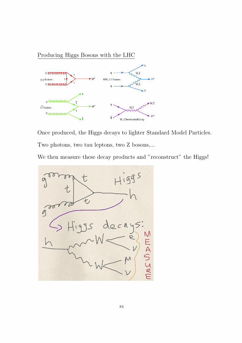
Producing Higgs Bosons with the LHC
Once produced, the Higgs decays to lighter Standard Model Particles.
Two photons, two tau leptons, two Z bosons,...
We then measure these decay products and ”reconstruct” the Higgs!
84

The above figure shows the branching ratios of the Higgs boson as afunction of its mass. These are the probablities for the Higgs to decayinto a certain set of particles as a function of its mass. Consisder theregion from 100 to 130 GeV. Here the decays are dominated by the bbfinal state. This is because the mass of the Higgs is not large enoughto decay into two Z bosons or W bosons or two top quarks. But it candecay into any of the other fermion/anti-fermion pairs. It decays into bbmost of the time because its coupling to bottom quarks is much largerthan that of any of the other fermions (except the top quark, but it can’tdecay to tt) because it doesn’t have enough mass.
As we increase the mass of the Higgs, beyond 130 GeV, decays intoW ’s become available and start to dominate until 180 GeV when Z’s alsoenter. Finally at twice the top quark mass, decays into tt are allowed anddominate.
The actual Higgs mass as measured by the LHC experiments is around125 GeV ± 2 GeV or so. This region is interesting because, with enough
85

data many of the final states are available and many have actually beenobserved. If the Higgs mass had turned out to be 190 GeV, only WWand ZZ would have been observable.
Notice that, even thought the Higgs is electrically neutral, that decaysto two photons i.e. γγ appear on the graph. These decays actuallyoccur due to higher order (one loop) processes in the Standard Model.This is why the γγ channel has a small branching fraction. However,even though it is small, experimentally it is easier to study than bb at ahadron collider. This is because the background to bb is much larger thanthat of γγ. In fact, the calorimeters of ATLAS and CMS were designedto find the Higgs boson in the γγ final state. These instruments turnedout to perform even better than anticipated and the Higgs was first seenin the γγ channel.
How is the mass of the Higgs measured in the diphoton channel?First, we select events with two photons and nothing else.We require that these photons are ”very clean” and have energies/momenta
of at least 15 GeV or so.Since we measure the energies and momenta of the photons, for each
such event we have a Lorentz 4-vector for each photon: P µ1 and P µ
2 .From these we construct the invariant mass squared:
M 2 = (P µ1 + P µ
2 )(P1µ + P2µ) = (E1 + E2)2 − (p1x + p2x)
2 − ... (317)
The reason for this is that, if the Higgs decays to two photons thenLorentz invariance implies that
P µh = P µ
1 + P µ2 (318)
i.e. that the Higgs’ Lorentz vector equals the sum of the Lorentz vectorsof the two photons and the Higgs Lorentz vector satisfies
P µhPhµ = m2
h (319)
Now, events with diphotons can be produced by many other processesleading to a large background to this search. But, if we understand
86

precisely enough the background and the signal-to-background rate islarge enough then we should be able to see the ”Higgs peak” above thebackground. This is an example of what has been seen:
You can see a clear peak in the data around 126 GeV.
87

SU(5) the Standard Model and Proton Decay
Consider the set of special, unitary, 5-by-5 matrices i.e. SU(5).This set contains both SU(3), SU(2) and U(1).SU(3) is the subset of of SU(5) matrices of the form:(
M3 00 1
)(320)
where M3 is a 3-by-3 SU(3) matrix, the 1 is the 2-by-2 identity matrixand the other entries are all zero.
Similarly, SU(2) is contained in the subset(1 00 M2
)(321)
Moreover, these SU(3) and SU(2) subsets of SU(5) commute with eachother. There is also a U(1) subset which commutes with both SU(3) andSU(2) subsets:
eiqθ 0 0 0 00 eiqθ 0 0 00 0 eiqθ 0 0
0 0 0 e−i32qθ 0
0 0 0 0 e−i32qθ
(322)
Note that the determinant is 1 implies that the sum of the five U(1)charges is zero.
The fact that the determinant of an SU(5) matrix is 1, implies that,when SU(5) acts on a 5-vector, the five charges of the 5-components ofthat vector under any U(1) subset will add to zero.
We have shown that the Standard Model gauge symmetry SU(3) ×SU(2) × U(1)Y is a subset of a ”simpler” symmetry SU(5). Could thisbe a useful idea to consider? Could the gauge symmetry of our worldbe SU(5)? This would be remarkable because the three SM couplingsg1, g2, g3 would be unified into one ”grand unified coupling” gGUT .
88
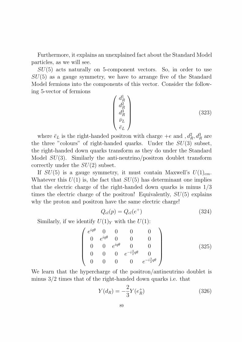
Furthermore, it explains an unexplained fact about the Standard Modelparticles, as we will see.SU(5) acts naturally on 5-component vectors. So, in order to use
SU(5) as a gauge symmetry, we have to arrange five of the StandardModel fermions into the components of this vector. Consider the follow-ing 5-vector of fermions
d1R
d2R
d3R
νLeL
(323)
where eL is the right-handed positron with charge +e and , d2R, d
3R are
the three ”colours” of right-handed quarks. Under the SU(3) subset,the right-handed down quarks transform as they do under the StandardModel SU(3). Similarly the anti-neutrino/positron doublet transformcorrectly under the SU(2) subset.
If SU(5) is a gauge symmetry, it must contain Maxwell’s U(1)em.Whatever this U(1) is, the fact that SU(5) has determinant one impliesthat the electric charge of the right-handed down quarks is minus 1/3times the electric charge of the positron! Equivalently, SU(5) explainswhy the proton and positron have the same electric charge!
Qel(p) = Qel(e+) (324)
Similarly, if we identify U(1)Y with the U(1):eiqθ 0 0 0 00 eiqθ 0 0 00 0 eiqθ 0 0
0 0 0 e−i32qθ 0
0 0 0 0 e−i32qθ
(325)
We learn that the hypercharge of the positron/antineutrino doublet isminus 3/2 times that of the right-handed down quarks i.e. that
Y (dR) = −2
3Y (e+
R) (326)
89

What about the other fermions?Well, we have already seen that SU(2) can be generated by 2-by-2
matrices (Pauli) and by 3-by-3 matrices (rotation generators). So, afixed symmetry can be realised by matrices of different dimensions. Infact, for SU(2) there are matrix representations of all sizes i.e. k-by-kwhere k is any integer. Similarly, the other symmetry groups SU(N) forN > 2 can also be generated by matrices whose sizes are larger than N -by-N . e.g. SU(3) can be generated by 6-by-6, 8-by-8 and larger matrices.For SU(5) which interests us here, after the 5-by-5 representation, thereis also a 10-by-10 one. Though there are lots of larger ones, these arethe two smallest sets of generators. The remarkable fact is that thesetwo representations ”explain” all of the charges of the Standard Modelfermions.
We usually denote the representations by their dimensions. So, forinstance the representation of SU(2) by the Pauli matrices is denoted asa 2 of SU(2); the 3 of SU(3) is the representation of SU(3 under whichthe quarks transform, and so on. So, under the Standard Model gaugesymmetry SU(3) × SU(2) × U(1)Y the fermions of a single generationtransform as
(3,2)1/3 + (3∗,1)−4/3 + (3∗,1)2/3 + (1,2)−1 + (1,1)2 (327)
Note that we have written the representation of all the left-handedfermions or anti-fermions since it makes sense to combine all the left-handed spinors together. The first term is the left handed, up-downquark doublet. This is because the left-handed quarks transform in the3 of SU(3), the u and d combine to transform as a 2 of SU(2) and thesubscript 1/3 is their hypercharge. The second term is the anti-up quark(hence the ∗ on the 3); this is the anti particle to the right handed upquark and is hence left-handed like the first term. The second is theanti-down quark. The third is the left-handed neutrino-electron doubletand the last is the (left-handed) anti-(right-handed) electron i.e. the lefthanded positron.
90

When we put the right-handed down quark and the right-handed anti-electron/neutrino doublet into the 5-vector, we learned that, under theSU(3)× SU(2)× U(1)Y subset of SU(5):
5 = (3,1)−2/3 + (1,2)1 (328)
Similarly we can consider the conjugate of this:
5∗ = (3∗,1)2/3 + (1,2∗)−1 (329)
Finally, the remarkable thing is that, if we take the ten-dimensionalrepresentation of SU(5), under the SM subset we have
10 = (3,2)1/3 + (3∗,1)−4/3 + (1,1)2 (330)
We therefore learn that
5∗ + 10 = (3,2)1/3 + (3∗,1)−4/3 + (3∗,1)2/3 + (1,2)−1 + (1,1)2 (331)
so that the two simplest representations of SU(5), when written interms of the SU(3)×SU(2)×U(1)Y subset reproduce exactly the chargesof all the Standard Model fermions!
We have thus far discussed how the Standard Model particles fit intoSU(5) representations. We have discussed the 12 ”directions” inside anSU(5) matrix which correspond to the 8+3+1=12 generators of SU(3)×SU(2) × U(1)Y . What about the ”other” elements of SU(5) which are*not* in SU(3) × SU(2) × U(1)Y ? SU(5) is 24-dimensional i.e. has24 generators and 24 gauge bosons. There are thus 12 gauge bosonspredicted by SU(5) which are *beyond* the Standard Model. Can weestimate the masses of these gauge bosons?
In order to do that we have to consider what sorts of interactions aremediated by these gauge bosons. To see those we should consider SU(5)transformations which are NOT in SU(3) × SU(2) × U(1)Y . Considerthe following example of an SU(5) transformation:
91

1 0 0 0 00 1 0 0 00 0 0 0 10 0 0 1 00 0 −1 0 0
d1R
d2R
d3R
νLeL
=
d1R
d2R
eLνL−d3
R
(332)
This interchanges a down quark with a positron! Therefore, the 12SU(5) gauge bosons which are not identified with Standard Model gaugebosons mediate interactions between quarks and leptons. If a quark canturn into a lepton by emitting an SU(5) gauge boson, then the proton(which is absolutely stable in the Standard Model) would become unsta-ble. Thus, the idea of grand unification of the fundamental forces predictsprotons will decay. We can estimate the lifetime of the proton in termsof the SU(5) coupling constant and the masses of the (fictitious) SU(5)gauge bosons. The diagram and the calculation are very similar to themuon decay calculation that we have done before.
92

The figure shows the analogy with muon decay in calculating theproton lifetime. The diagram on the right shows a process in whichp→ π0e+. The two u-quarks in p annihilate into the SU(5) gauge bosonX. X then decays into e+, d via the interaction we described above. Atthis point, the d-quark combines with the produced d to make a neutralhadron, the pion.
The basic matrix element comes from the uu→ X → e+d part of thediagram and
M∝ g2GUT
M 2X
(333)
where gGUT is the SU(5) gauge coupling and MX the mass of the gaugeboson. Thus the decay width
Γ(p→ e+π0) ∝ |M|2 ∼ g4GUT
M 4X
(334)
This is a very low momentum process relative to MX . Since the protonmass is much larger than both the pion and positron masses, the onlyother relevant scale in the problem is the proton mass mp. Since Γ hasmass dimension [M ]1 it must be that
93

Γ(p→ e+π0) ∼g4GUTm
5p
M 4X
(335)
We can thus use this formula, together with the experimental limit onthe lifetime of the proton to constrain the combination M ≡ MX
gGUT, though
in practice gGUT is not usually that small so effectively we constrain MX .
Measuring/Setting a limit on the proton lifetime
The current limit on the proton lifetime for the decay mode we areconsidering is about τp > 1.6× 1033 years!
Q: How can we obtain such a strong limit, 23 orders of magnitudelonger than the age of the Universe (about 1010 years) ?
94

A: By watching a very large number of protons for as long as possibleand seeing that none have decayed yet!
One way to look for proton decay is to surround a tank of water with”photon detectors ” ie photo multiplier tubes. The positron will interactwith the electrons in the water to produce photons and the π0 almostalways decays to two photons.
Since 1m3 of water contains around 1030 protons, if no protons areobserved to decay after one year we get a limit of about 1030 years.So, by putting photo-multiplier tubes around larger amounts of waterone can obtain a stronger limit. The SuperKamiokande experiment has50,000 tons of water and this is where the best limit on the proton lifetimecomes from.
SuperK also detects neutrinos: when a neutrino comes in to the waterit can sometimes exchange a Z-boson with an electron in the water. Ifthe original neutrino is energetic enough, the electron will recoil withhigh enough momentum such that it will travel faster than the speedof light in water. When this happens, the electron will emit what iscalled Cerenkov radiation, which are photons which can be detected inthe photomultiplier tubes. Similarly, if the incoming neutrino exchangesa W -boson with an electron or quark in the water, it will convert intoan electron, muon (or tau if energetic enough) and this could also emitCerenkov light if fast enough.
95

We therefore have that
M 4
m5p
> 1.6× 1033yrs = 50.5× 1039s = 7.65× 1064(GeV )−1 (336)
Approximating mp ∼ 1GeV we have that
M 4 > 7.65× 1064GeV (337)
or
M > 1.7× 10¹⁶GeV (338)
In other words we obtain a limit on the mass scale which is 16 ordersof magnitude larger than the proton mass, 14 orders of magnitude largerthan the masses of the W and Z bosons! This very large scale of order1016 GeV is known as the GUT scale – the scale of grand unification. IFgrand unification is correct, it is at this scale that the additional bosonspredicted by grand unification get their masses i.e. the SU(5) symmetryis broken at a very high scale.
Anyway, from the point of view of the course, the idea behind thiscalculation is to give a) in idea about how theoretical physics think –using the idea of gauge symmetry and pushing it to its final conclusions
96

and b) to show how one can use the experimental data to get an idea ofwhat theoretical parameters have to be and c) to understand the basicidea behind proton decay experiments.
97