ElementsAn object oriented approach to industrial software development

Gerd Baumann* and Michal Mnuk†

* Department of Mathematical PhysicsUniversity of UlmAlbert-Einstein-Allee 11D-89069 Ulmgerd.baumann@physik.uni-ulm.de

† Institute of InformaticsTechnical University of MunichBoltzmannstrasse 385748 Garching b. Münchenmnuk@in.tum.de

Abstract: This article discusses an object oriented approach to industrial softwaredevelopment using Mathematica. We present the package Elements for structuredrepresentation of physical, engineering, and mathematical objects. This packageintroduces object oriented paradigms into Mathematica and is used to develop amodeling environment built on a knowledge base where classes' and objects'properties and relations are maintained in a consistent, transparent, andextensible way. We show how this tool can be applied to design modelsparametrized by structured objects instead of just simple values.

à Introduction

Mathematica as the leading calculation tool for symbolic calculations offers a broad mathematical

and programming functionality. There are more than 1800 functions in version 4.2 available to set

up a program or carry out a calculation. The mathematical and programming approach to a

computer algebra system is well accepted and very useful for a trained user with a sound background

in physics or engineering. The strength of Mathematica lies in its consistent and versatile

functionality that allows to tackle an engineering problem right from the scratch. This approach to

solve a problem starting with the fundamentals is used traditionally by physicists as well as

engineers at universities. However, in the industrial environment there is a large group of potential

users lacking of time to acquire the complete knowledge of all the versatile possibilities that

Mathematica offers. The mismatch between the requirements of a sophisticated calculation tool and

the rather limited knowledge of an average user is a great obstacle in the industrial application of

Mathematica.

Another point frequently brought up in talks with engineers about calculation tools, especially for

engineering purposes, is the lack of ability to manage tasks in an "intuitive" graphical interaction.

Thus, our experience from many communications with engineers is that Mathematica is a very

powerful tool with a huge source of mathematical functionality but with a relatively poor interface to

an industrial developer or user.

A sophisticated programmer uses Mathematica with great excellence and knowledge on a specific

functionality. However, a standard user in the industrial environment does not have the time nor the

passion to first read several hundred pages of the manual in order to be able to solve a problem. The

tight time frame in projects dictates that an industrial developer has to handle two tasks with

different priorities simultaneously and efficiently: the higher priority is assigned to the description

and generation of the model while the implementation or programming in Mathematica or in other

tools comes next. In a standard development process these two tasks concur with each other. If any

of these two tasks is supported by efficient methods and can be accomplished with less effort, the

developer will save time and money.

Our experience from many discussions with engineers is that the creation of a model takes a cerain

amount of time that strongly depends on the accuracy and the complexity with which some effects

and properties of the real system are described. Based on this model, the coding in Mathematica

takes still a considerable amount of time which can be reduced if a standard programming

environment is available to the programmer. In the industrial environment it is essential to have a

clear cut definition of the development process. There is no room for probing for the best

development strategy since the competition on the market dictates a tough schedule. Thus, it is

imperative to set up the development process in an as much efficient way as possible. The tools used

in such a process should basically reflect or, more precisely, represent the main features of a model.

Models in engineering as well as in physics, chemistry, finance, mathematics, and economics are

characterized by two main features:

First, any model is based on methods representing an algorithm with which the problem issolved. These methods usually depend on each other or are at best completely independent.

The second feature of any model is the occurrence of parameters determining the physical,engineering, economic, etc. properties and thus the behavior of the system.

The parameters are of central importance when variations of the model are examined. For example

these quantities determine bifurcations to different states of the system. By variations we mean not

only numeric changes but also the symbolic ones.

However, modeling is a sophisticated endeavor of traversing between reality, imagination and

feasibility. It eventually converges to a mathematical description which captures the most essential

aspects important for a particular purpose and, at the same time, it is simple enough to be treated by

formal methods.

We start with an observation that every modeling process involves working with objects and its

primary goal is to select features relevant to a specific problem together with relations between

them. Different problems in one specific area usually involve a rather limited number of objects. The

problem itself is then reflected in the relations between them.

From this point of view it is natural to build a knowledge base containing descriptions of basic

objects which often appear in modeling. Such a database would significantly speed up the modeling

and provide a basis for rapid prototyping. It is not only a tedious and error prone task to type in

2 G. Baumann

things over and over again. In many cases, parametrized solutions for recurring problems could be

computed and stored in advance.

Our primary motivation is to facilitate the modeling process in engineering by providing a

transparent and easy-to-use knowledge base of objects. In this paper we stipulate and analyze

requirements on such a system and present a Mathematica package to store and retrieve

informations about objects.

The proposed system is designed to be, in its nature, primarily static. It is not supposed to include

``automatic solvers'' although internal and external algorithms will be utilized to perform

computation whenever this appears appropriate. Extensions of the knowledge base will always be

checked by a human. The reason is that the vast majority of practical problems does not provide for

easy answers. Even though today's computer systems became very powerful, automatically obtained

solutions still need to be post-processed by experts. This makes it impossible to simply add them to

an existing knowledge base since sooner or later its consistency would inevitably be destroyed

making it useless.

à Objects in ModelingWhen we analyze requirements on the design of a system for object representation, we naturally

come across some principles already used for years in software engineering - the object oriented

programming. It is not surprising that the same or very similar principles will govern the design

here.

Object oriented programming introduced the concept of classes and inheritance. It can be observed

that solutions often simplify considerably when a hierarchical structure was imposed on problems.

Another aspect of object oriented programming may be even more important. Classes and their

objects are encapsulated, stand-alone and well specified entities which behave the same way in any

program - this is a key property of reusable components. This makes it possible to publish code

which can be used in various settings without change.

It is clear that these paradigms apply to modeling as well. A hierarchical structure is already in the

nature of all mathematical and physical objects while the closeness of used entities is a prerequisite

for the use of objects in different environments. These two concepts will play a primary role in the

design of a modeling environment.

à Object Oriented Methods in Computer AlgebraThe fact that principles of object oriented programming are compatible with structures in scientific

computing led to adoption of object oriented design methods in computer algebra systems. A proper

combination of these two fields yields the key to a solution of our problem. On the one hand, object

oriented design provides for encapsulation and reusability of objects, on the other hand, computer

algebra offers a variety of algorithms to work with them.

However, up to now there is no single system that would contain these features in a well balanced

symbiosis. We encounter either systems offering implementation of the class concept (C++, Java,

SML, Aldor, ...), or single- or multi-purpose (computer algebra) systems providing more or less

large set of algorithms (Maple, Mathematica, GAP,...).

Despite of this fact, lot of successful work was already done on using object oriented methods in

computer algebra. There is an extensive literature on object oriented numerical methods [1, 2, 3, 4].

Numerical algorithms benefit from the fact that most of data types they work on are largely

Elements

supported by classical programming languages so there are quite a few choices. However, numerics

does not belong to areas that would primarily benefit from object oriented paradigms.

Another approach integrates object oriented programming languages and computer algebra in one

application [5, 6, 7, 8]. However, these solutions are mostly aimed at a few specialized fields.

The last option is to stay solely within a computer algebra system. Maple was for a long time

lacking a proper concept for data encapsulation. It was finally included in Version 7. An example of

object oriented programming in numerical computation in Maple can be found e.g. in [9]. Despite of

this, Maple's imperative nature is not well suited for complex manipulations on data and code that is

necessary when implementing object oriented features.

Probably the first implementation of classes in Mathematica was done by R. Maeder in [10]. Even

though this code was just a proof of concept, it demonstrated the strength of the language and

proved that Mathematica provides powerful means for building structures and for data

encapsulation.

Applications in engineering require an extensive collection of algorithms which is currently

provided only by general computer algebra systems like Mathematica or Maple. In this paper we

present the package Elements which provides an implementation of object oriented features to

facilitate modeling directly within Mathematica. The package goes beyond Maeder's work and it

proved to be well suited for the purpose of building a knowledge base of objects from which models

are built. In the next section, we postulate and analyze requirements on a working environment for

rapid development of models in engineering.

à Design RequirementsThe package Elements is supposed to support and facilitate the modeling process by providing an

efficient working environment. This is the primary goal which all other requirements specified

below are emanating from.

Even though the focus has been put on the object oriented approach, we want to stress that our

intension is not to mimic paradigms found in other object oriented programming languages. The

capabilities of Mathematica will be enhanced only to an extent that is necessary to achieve the

specified goals for industrial applications.

Hierarchical Structure

We already argued that there is no apparent reason for a knowledge base to have a particular

structure. But it is a fact that human beings try to organize things into categories. This gives rise to

hierarchies which make the relations between categories and objects more comprehensible.

Similarly as in object oriented programming, the key role in our approach is played by classes. They

represent different abstraction levels of objects. Classes at higher levels describe general principles

which are ``specialized'' on the way down in the hierarchy. Subordinate classes inherit properties of

their ancestors, they may restrict or modify them and/or introduce new ones. Classes serve as

templates for creating objects. However, they will often be used on their own.

We stipulate:

4 G. Baumann

Classes are organized in hierarchies such that every class has exactly one ancestor (superclass).They serve as templates for creating objects.

This principle enables us to provide an exact, concise and well defined description of objects.

Reusability of Objects

One of our primary design goals is to achieve reusability of objects - the ability to be transparently

used in different settings. This, at least, presumes that objects are represented in a way that makes

them independent of their environment. The next stipulation is:

Represented objects can be easily imported and used in different environments. The behavior ofobjects does not depend on a specific environment.

Soundness of Representation

When a programmer wants to use a piece of code written by someone else, he needs a clear

understanding about what this code expects as input and what it yields on output. While this can be

rather easily fulfilled in classical programming languages, more care needs to be taken when

dealing with complex objects in computer algebra. Usually, the input and output of functions

implemented in programming languages is determined by the underlying type system which is in

most cases quite simple.

A knowledge base built upon the package Elements will store models of objects, for example metal

rods. Suppose, this representation contains certain physical properties of rods together with a

function describing the bending when force is applied. As this information may depend on various

assumptions which cannot be deduced from the properties of a rod itself (like some simplifications

that were done while solving the differential equation describing the bending), a proper use of the

model is possible only if all restrictions are known to the user. Hence, they must be properly

represented and stored with the modeled objects. We require:

Represented objects are accompanied with a sufficient amount of information that makeschecking the validity of the stored data possible.

Consistency of Representation

It is obvious that introducing inconsistencies or contradictions into a system that stores knowledge

makes it unusable. Hence, even if the soundness of the represented data is established, in the course

of working with the data this state must be preserved. Hence:

The system provides suitable means to check the consistency of the stored data.

Elements

In the ideal case, these means are used to automatically obtain statements about constraints and

validity of new classes and objects. They ensure that subclasses are properly constructed and that

they obey restrictions imposed by parent classes. If automatic validity checking is not possible or

feasible, the user must be able to extract enough information from the object representation to

perform this task by hand.

Data Exchange

We require that a knowledge base can be easily integrated into existing environments and that it

must be capable of communicating with other aplications using standard protocols:

The knowledge base is able to import and export data and communicate with other systems.

This opens the possibility to incorporate the stored information into other systems as an add-on for

essentially no extra work. On the other hand, the knowledge base will benefit from any external

information that may be available.

à Elements - A Tool for Representing Objects in MathematicaAfter we have specified basic requirements to be satisfied, we present a brief survey on current

capabilities of the package Elements. The first two subsections illustrate the implementation of

standard notions of class and inheritance. Then, we apply these paradigms to two problems -

modeling a car driving on a bumpy road and, a more mathematical subject, the dynamics in Poisson-

Hamilton manifolds.

Classes and Objects

A class is a structure consisting of properties and methods. Properties represent constant features of

objects while methods are the usual functions. Both properties and methods may be associated with

attributes that are used as denotational items. Properties, attributes and methods are kept inside of

classes and they do not interfere with the environment. But, all features of the current session in

which objects are defined (especially the complete functionality of Mathematica) are accessible from

within classes.

There is a distinguished class Element which is the root of the whole hierarchy. New classes are

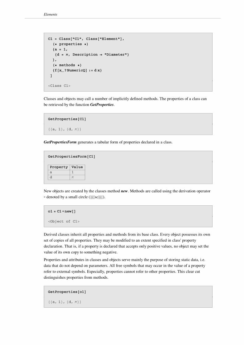
derived from existing ones. Below, the class C1 (the name is specified in the first argument of the

function Class) is derived from the class Element. It has properties a and d (there is one attribute

called Description associated with d) and a method f defined for numeric arguments.

6 G. Baumann

C1 = Class@"C1", Class@"Element"D,H∗ properties ∗L8a = 1,

8d = π, Description → "Diameter"<<,H∗ methods ∗L8f@x_?NumericQD := d x<

D

<Class C1>

Classes and objects may call a number of implicitly defined methods. The properties of a class can

be retrieved by the function GetProperties.

GetProperties@C1D88a, 1<, 8d, π<<GetPropertiesForm generates a tabular form of properties declared in a class.

GetPropertiesForm@C1D

Property Value

a 1

d π

New objects are created by the classes method new. Methods are called using the derivation operator

ë denoted by a small circle (ÂscÂ).

o1 = C1Înew@D

<Object of C1>

Derived classes inherit all properties and methods from its base class. Every object possesses its own

set of copies of all properties. They may be modified to an extent specified in class' property

declaration. That is, if a property is declared that accepts only positive values, no object may set the

value of its own copy to something negative.

Properties and attributes in classes and objects serve mainly the purpose of storing static data, i.e.

data that do not depend on parameters. All free symbols that may occur in the value of a property

refer to external symbols. Especially, properties cannot refer to other properties. This clear cut

distinguishes properties from methods.

GetProperties@o1D88a, 1<, 8d, π<<

Elements

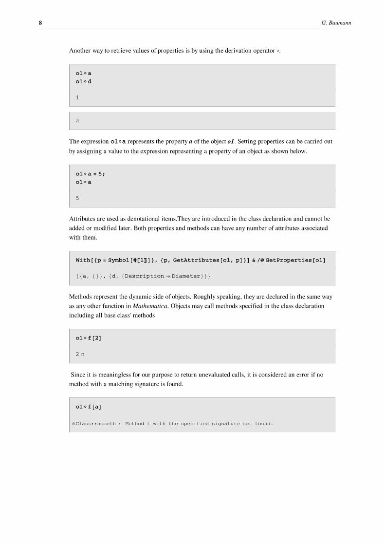
Another way to retrieve values of properties is by using the derivation operator ë:

o1Îa

o1Îd

1

π

The expression o1Îa represents the property a of the object o1. Setting properties can be carried out

by assigning a value to the expression representing a property of an object as shown below.

o1Îa = 5;

o1Îa

5

Attributes are used as denotational items.They are introduced in the class declaration and cannot be

added or modified later. Both properties and methods can have any number of attributes associated

with them.

With@8p = Symbol@#P1TD<, 8p, GetAttributes@o1, pD<D & ê@ GetProperties@o1D88a, 8<<, 8d, 8Description → Diameter<<<Methods represent the dynamic side of objects. Roughly speaking, they are declared in the same way

as any other function in Mathematica. Objects may call methods specified in the class declaration

including all base class' methods

o1Îf@2D

2 π

Since it is meaningless for our purpose to return unevaluated calls, it is considered an error if no

method with a matching signature is found.

o1Îf@aD

‹Class::nometh : Method f with the specified signature not found.

8 G. Baumann

Derived Classes and Inheritance

An important paradigm implemented in the package Elements is that of derived classes and

inheritance. Every class must have a base class from which it inherits all properties and methods. It

can then override the old or add new properties and methods. If a derived class declares a property

or a method which already exists, the old property or method will be "shadowed" by the new

declaration (i.e. it becomes invisible).

The class C2 below serves as a base class for C3 which overrides the property a and adds a new

definition for the method f with two arguments.

C2 = Class@"C2", Class@"Element"D,8a = 1, b = 2<,8f@x_D := x^2, g@x_D := a f@xD<

D

<Class C2>

C3 = Class@"C3", C2,

8a = π<,8f@x_, y_D := a x y<

D

<Class C3>

A newly created object of C2 will be initialized according to the declarations given in C2 while the

property a of a newly created object of C3 will get the initial value p that was introduced in the

declaration of C3.

o2 = C2Înew@D;GetProperties@o2D88a, 1<, 8b, 2<<o3 = C3Înew@D;GetProperties@o3D88a, π<, 8b, 2<<

The value of a in the body of g refers to the current value stored in the object that g was invoked

with.

Elements

o2Îg@3D

9

o3Îg@3D

9 π

An object of the class C3 can refer to the shadowed value of a from the class C2 by C2Îa.

C2Îa

1

Methods are inherited in a similar way as properties. If a derived class declares a method with the

same name and signature as one of its ancestor classes, the old declaration will be "shadowed" by

the new one. If the name is the same but the signature differs, a new definition is associated with

that name.

In the above example, the class C3 contains a declaration of the method f with two arguments. This

definition is associated with the symbol f that was introduced in C2. Hence, objects of the class C3

may call f with one or two arguments while for objects of C2 only the method f with one argument

is known.

o3Îf@3D

9

o3Îf@3, 4D

12 π

o2Îf@3, 4D

‹Class::nometh : Method f with the specified signature not found.

The functionality of the package Elements goes beyond that what was described in this section. We

refer to the package documentation for further details.

10 G. Baumann

Examples

à Car on a Bumpy RoadThe problem considered here is a practical application originating from the early phase of a car

design process. Engineers in the automotive business have to know in advance how a new car will

react under certain environmental conditions. In the sequel, we discuss a procedure to build a model

to provide basic information on the behavior of a car at the very beginning of the design. In this

early stage of the process, very few information on the new car is available and thus it is sufficient to

reduce the model to the most essential properties of the car. For example, these properties include

the mass distribution on a chassis; i.e the location of the engine and other heavy components like the

fuel tank, batteries, gear box, etc. Another essential feature in this early design phase is the

undercarriage. In our model, we combine these components to a multi body system interacting by

forces with each other and with the environment. Knowing the preliminary behavior of the new car,

the next step is to improve the model in several iterations incorporating more and more details of

the interacting components. Here, we restrict our considerations to the very beginning of the design

process and demonstrate how an object oriented approach can be used to model different

components in a transparent way.

The figure below shows the simplified one dimensional mechanical model of a car moving on a

bumpy road. In principle, the car consists of three main components - the two axes and the car body.

We assume that the two axes are coupled to the chassis by a dashpot and a spring. In addition to the

translation we allow a narrow rotation of the body. The wheels are in contact with the road (this

interaction is modeled by introducing springs and dampers representing the two tires). The symbols

shown in the figure have the following meaning: ki , di with Hi = 1 - 4L , mk with Hk = 1, 2, 3L , a ,

and b are the physical and geometric parameters of the system. The ki and di denote force and

damping constants, mk are the wheel and chassis masses, and a , b determine the center of the mass

of the chassis. JC2 = I is the inertia moment of the chassis. The dynamical coordinates denoted by

z1 , z2, z3 and b describe the vertical and angular motion of the car. The acting external forces on

the car are due to bumps in the road and due to gravitation. Now, the whole system can be described

by Newton's equations.

Elements

These equations are given for the coordinates by

(1)m1 z1´´ = -F1 + F3

(2)m2 z2´´ = -F2 + F4

(3)m3 z3´´ = F3

(4)I b´´ = b F3 - a F4

where Fi are the acting forces. One of the main problems in car design is to estimate how the total

system will react under different forces, under different damping parameters, under different

velocities, under different environment conditions, etc. These questions are partially answered in the

following subsections. The complete examination of all these inquiries would exceed the space

available for this article. Hence, we will restrict our consideration to a few examples.

To attack the physical and mathematical problem we first identify classes that would capture the

essence of this problem. If one looks at the equations of motion and at the above figure, it seems

natural to divide the car into three main classes - the body, the axes and the environment.

Class Definitions

The problem can be split into the following classes - the general setup class, the car body, the axes,

the car itself, and some tools needed to carry out the simulation. The simulation class that provides

graphical output to the user refers to other classes that serve as a basis of the computation required

to produce the output.

ü General Setup

The general setup is concerned with geometric properties and the influence of the environment, such

as the external force characterized here by four bumps in the road.

Setup = Class@"Setup", Class@"Element"D,88a = 1.2, Description → "distance front axis"<,8b = 1.2, Description → "distance rear axis"<,8v = 5, Description → "velocity of the car"<,8stepWidth = 0.1`, Description → "step width"<,8stepHeight = 0.07, Description → "step height"<<,

8extForce@t_D :=

Fold@Plus, 0, Table@HTanh@100 ∗ v ∗ Ht − n stepWidthLD − Tanh@100 ∗

Hv ∗Ht − n stepWidthL − stepWidthLDL ∗ stepHeightê 2, 8n, 1, 4<DD<D

<Class Setup>

12 G. Baumann

ü Body

The class Body consists solely of geometric and physical parameters of the car body. This class

includes also the initial conditions for displacement, angle and velocity.

Body = Class@"Body", Setup,

8description = "Body",

8m = 1200, Description → "mass"<,8z0 = 0, Description −> "initial displacement"<,8zp0 = 0, Description −> "initial velocity"<,8h = 0.75, Description → "geometric quantity"<,8β0 = 0, Description −> "initial value for β"<,8βp0 = 0, Description −> "initial value for β prime"<,8zFunName = z, Description → "name of the z function"<,8betaFunName = β , Description → "name of the β function"<<,

8<D

<Class Body>

ü Axes

The common properties of the two axes are collected in the class CarAxis. This class contains only

parameters - force and damping constants together with initial conditions for the equations of

motion.

CarAxis = Class@"CarAxis", Setup,

8description = "Axis",

8m = 42.5, Description → "mass of the axis"<,8k1 = 150000, Description → "wheel−body force constant"<,8d1 = 700, Description → "wheel−body damping constant"<,8k2 = 4000, Description → "wheel−road force constant"<,8d2 = 1800, Description → "wheel−road damping constant"<,8z0 = 0, Description → "initial displacement"<,8zp0 = 0, Description → "initial velocity"<,8zFunName = z, Description → "name of the function z"<<,

8<D

<Class CarAxis>

In the next step we define classes for the front and the rear axis. The front axis consist solely of a

method generating the equation of motion for the axis by considering the acting forces.

Elements

FrontAxis = Class@"FrontAxis", CarAxis,

8<,8getEquations@body_ ê; ObjectOfClassQ@body, BodyDD :=

Block@8f1 = k1 ∗ HzFunName@tD − extForce@tDL +

d1 ∗ HzFunName'@tD − D@extForce@tD, tDL,f3 = k2 ∗ HHbodyÎzFunNameL@tD − b ∗ HbodyÎbetaFunNameL@tD

− zFunName@tDL + d2 ∗ HD@HbodyÎzFunNameL@tD −

b∗ HbodyÎbetaFunNameL@tD, tD − zFunName'@tDL<,8m ∗ zFunName''@tD + H−f1 + f3L ∗ −1 0,

zFunName@0D z0, zFunName'@0D zp0<D<

D

<Class FrontAxis>

The rear axis is generated in the same way by taking the relations specific for this component into

account.

RearAxis = Class@"RearAxis", CarAxis,

8<,8getEquations@body_ ê; ObjectOfClassQ@body, BodyDD :=

Block@8f2 = k1 ∗ HzFunName@tD − extForce@t − Ha + bL ê vDL +

d1 ∗ HHbodyÎzFunNameL'@tD − D@extForce@t − Ha + bL ê vD, tDL,f4 = k2 ∗HHbodyÎzFunNameL@tD + a ∗ HbodyÎbetaFunNameL@tD

− zFunName@tDL + d2 ∗ HD@HbodyÎzFunNameL@tD +

a ∗ HbodyÎbetaFunNameL@tD, tD − zFunName'@tDL<,8m ∗ zFunName''@tD + H−f2 + f4L ∗ −1 0,

zFunName@0D z0, zFunName'@0D zp0<D<

D

<Class RearAxis>

ü Car

Finally, after setting up classes for the body and axes, we define a class to describe the car. This

class incorporates parameters as well as methods to combine information from different components.

14 G. Baumann

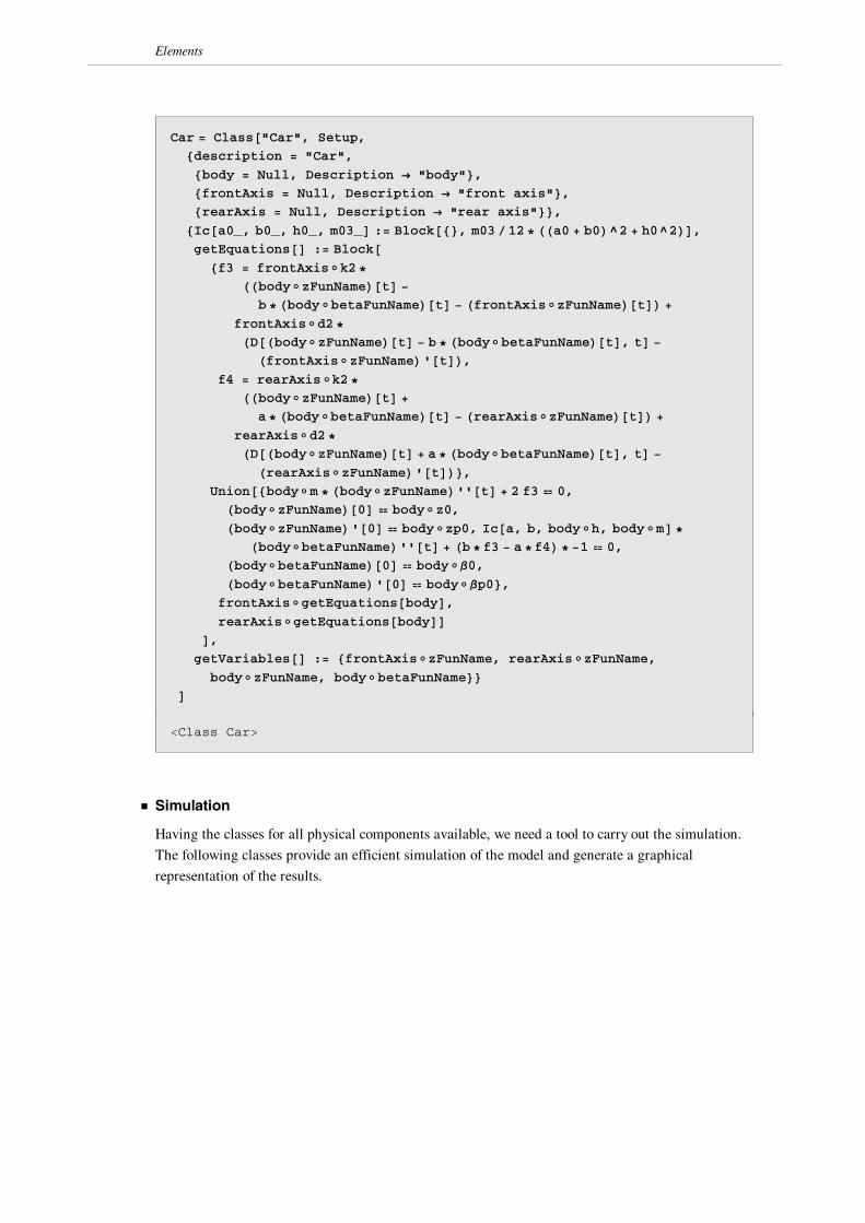
Car = Class@"Car", Setup,

8description = "Car",

8body = Null, Description → "body"<,8frontAxis = Null, Description → "front axis"<,8rearAxis = Null, Description → "rear axis"<<,

8Ic@a0_, b0_, h0_, m03_D := Block@8<, m03 ê 12 ∗ HHa0 + b0L^2 + h0^2LD,getEquations@D := Block@

8f3 = frontAxisÎk2 ∗

HHbodyÎzFunNameL@tD −

b ∗HbodyÎbetaFunNameL@tD − HfrontAxisÎzFunNameL@tDL +

frontAxisÎd2 ∗

HD@HbodyÎzFunNameL@tD − b ∗ HbodyÎbetaFunNameL@tD, tD −

HfrontAxisÎzFunNameL'@tDL,f4 = rearAxisÎk2 ∗

HHbodyÎzFunNameL@tD +

a ∗ HbodyÎbetaFunNameL@tD − HrearAxisÎzFunNameL@tDL +

rearAxisÎd2 ∗

HD@HbodyÎzFunNameL@tD + a ∗ HbodyÎbetaFunNameL@tD, tD −

HrearAxisÎzFunNameL'@tDL<,Union@8bodyÎm ∗ HbodyÎzFunNameL''@tD + 2 f3 0,

HbodyÎzFunNameL@0D bodyÎz0,

HbodyÎzFunNameL'@0D bodyÎzp0, Ic@a, b, bodyÎh, bodyÎmD ∗

HbodyÎbetaFunNameL''@tD + Hb ∗ f3 − a ∗f4L ∗ −1 0,

HbodyÎbetaFunNameL@0D bodyÎβ0,

HbodyÎbetaFunNameL'@0D bodyÎβp0<,frontAxisÎgetEquations@bodyD,rearAxisÎgetEquations@bodyDD

D,getVariables@D := 8frontAxisÎzFunName, rearAxisÎzFunName,

bodyÎzFunName, bodyÎbetaFunName<<D

<Class Car>

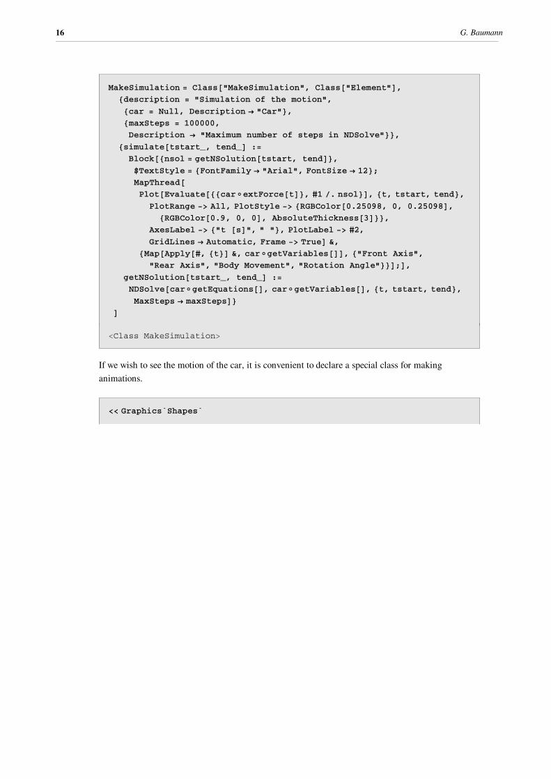
ü Simulation

Having the classes for all physical components available, we need a tool to carry out the simulation.

The following classes provide an efficient simulation of the model and generate a graphical

representation of the results.

Elements

MakeSimulation = Class@"MakeSimulation", Class@"Element"D,8description = "Simulation of the motion",

8car = Null, Description → "Car"<,8maxSteps = 100000,

Description → "Maximum number of steps in NDSolve"<<,8simulate@tstart_, tend_D :=

Block@8nsol = getNSolution@tstart, tendD<,$TextStyle = 8FontFamily → "Arial", FontSize → 12<;MapThread@Plot@Evaluate@88carÎextForce@tD<, #1 ê. nsol<D, 8t, tstart, tend<,

PlotRange −> All, PlotStyle −> 8RGBColor@0.25098, 0, 0.25098D,8RGBColor@0.9, 0, 0D, AbsoluteThickness@3D<<,

AxesLabel −> 8"t @sD", " "<, PlotLabel −> #2,

GridLines → Automatic, Frame −> TrueD &,8Map@Apply@#, 8t<D &, carÎgetVariables@DD, 8"Front Axis",

"Rear Axis", "Body Movement", "Rotation Angle"<<D;D,getNSolution@tstart_, tend_D :=

NDSolve@carÎgetEquations@D, carÎgetVariables@D, 8t, tstart, tend<,MaxSteps → maxStepsD<

D

<Class MakeSimulation>

If we wish to see the motion of the car, it is convenient to declare a special class for making

animations.

<< Graphics`Shapes`

16 G. Baumann

MakeAnimation = Class@"MakeAnimation", Class@"Element"D,8description = "Animate the motion of the car"

8path = "C:êMmaêWORKêTUMObjectsêElements05êLibraryêCarsêEEVCMediumêGeneric", Description −> "Path of the car model"<<,

8animate@sim1_, tstart_, tend_, δt_D :=

Block@8names, l1, tire1, tire2, window1, window2, window3, body,

sol = sim1ÎgetNSolution@tstart, tendD<,SetDirectory@pathD;names = FileNames@"∗.∗"D;l1 = Map@ReadList@#, Number, RecordLists → True,

RecordSeparators →

8If@StringMatchQ@$OperatingSystem, "Windows∗"D,"\n", "\r"D<D &, namesD;

tire1 = 8GrayLevel@0.752941D, Polygon@l1P1T ê. 8x_, y_< −> 8x, y + z1@tD<D<;

tire2 = 8GrayLevel@0.752941D, Polygon@l1P2T ê. 8x_, y_< −> 8x, y + z2@tD<D<;

window1 = 8GrayLevel@0.752941D, Polygon@l1P3T ê. 8x_, y_< −> 8x Cos@−β@tDD + y Sin@−β@tDD,

y Cos@−β@tDD − x Sin@−β@tDD + z3@tD<D<;window2 = 8GrayLevel@0.752941D, Polygon@

l1P4T ê. 8x_, y_< −> 8x Cos@−β@tDD + y Sin@−β@tDD,y Cos@−β@tDD − x Sin@−β@tDD + z3@tD<D<;

window3 = 8GrayLevel@0.752941D, Polygon@l1P5T ê. 8x_, y_< −> 8x Cos@−β@tDD + y Sin@−β@tDD,

y Cos@−β@tDD − x Sin@−β@tDD + z3@tD<D<;body = 8RGBColor@0, 0, 0.25098D, Polygon@

l1P6T ê. 8x_, y_< −> 8x Cos@−β@tDD + y Sin@−β@tDD,y Cos@−β@tDD − x Sin@−β@tDD + z3@tD<D<;

Table@Show@Graphics@8body, tire1, tire2, window1, window2,

window3< ê. solD, AspectRatio −> Automatic, Axes −> False,

Frame −> True, PlotRange −> 88−.1, 4.4<, 80, 1.4<<,FrameTicks −> NoneD, 8t, tstart, tend, δt<D;

D<D

<Class MakeAnimation>

Objects

Up to this point, nothing more than a framework was defined in which the computation can be

carried out. The classes represent essentially only templates for creating the real and calculation

objects. In order to setup the simulation, we have to generate objects and specify their properties.

The car is generated by a modular process incorporating the distinguished objects. At this point, it is

apparent that we have a great advantage in designing a specific car compared to traditional

approaches in simulation. For example, we can define different objects for axes and use them as in

different simulations as parameters of the underlying model. Components (objects) of the same type

can be exchanged without causing any harm to the system. In the sequel, we demonstrate how this

process is carried out.

Elements

ü Body

First, we create the body by calling the method new of the class Body. All properties except

zFunName and betaFunName will have their default valued specified in the class declaration.

b = BodyÎnew@8zFunName → z3, betaFunName → β<D

<Object of Body>

The actual properties of the body can be checked by

GetPropertiesForm@bD

Property Value

description Body

a 1.2

b 1.2

betaFunName β

h 0.75

m 1200

stepHeight 0.07

stepWidth 0.1

v 5

z0 0

zFunName z3

zp0 0

β0 0

βp0 0

ü Axes

Next, objects for the axes are created. The front axis is defined with a mass of 45.5 kg, the function

representing the displacement of the center of the wheel attached to this axis is denoted by z1 .

fa = FrontAxisÎnew@8m −> 45.5, zFunName → z1<D

<Object of FrontAxis>

The properties of the axis can be printed by:

18 G. Baumann

GetPropertiesForm@faD

Property Value

description Axis

a 1.2

b 1.2

d1 700

d2 1800

k1 150000

k2 4000

m 45.5

stepHeight 0.07

stepWidth 0.1

v 5

z0 0

zFunName z1

zp0 0

Since no values for the damping and the force constant were given in the call to new, these

properties are initialized with values specified in the class declaration.

A second version of the front axis with a more stiffer damping is derived in the following line. Here,

k1 and k2 were given different initial values.

fas = FrontAxisÎnew@8m → 45.5,

d1 → 5000, d2 → 5000,

k1 → 150000, k2 → 150000,

zFunName → z1<D

<Object of FrontAxis>

For the rear axis we just use the default settings. The coordinate of elongation is denoted by z2 .

ra = RearAxisÎnew@8zFunName → z2<D

<Object of RearAxis>

A check of parameters shows the default values.

Elements

GetPropertiesForm@raD

Property Value

description Axis

a 1.2

b 1.2

d1 700

d2 1800

k1 150000

k2 4000

m 42.5

stepHeight 0.07

stepWidth 0.1

v 5

z0 0

zFunName z2

zp0 0

ü Car

Having all needed components available, it is easy to generate the car by incorporating the defined

objects into a common model. The car object is defined by

c = CarÎnew@8frontAxis → fas, rearAxis → ra, body → b<D;

It consist of the front axis, the rear axis, and the body. We want to stress that the object oriented

design allows the behavior of the model to be modified very easily by changing different components

or their properties. Hence, if an engineer would have access to a collection of different bodies, axes

and other objects, he would be able to create and test many different car designs without the need to

adapt the model.

Simulation

A simulation object is created from the class MakeSimulation. The simulation can be performed

with any object of the class Car that is assigned to the property car in the call to the method new.

sim = MakeSimulationÎnew@8car → c<D

<Object of MakeSimulation>

Finally, the actual simulation is initiated by calling the simulate method of the class

MakeSimulation. The input for this function are just the starting point and the end point of the

simulation interval. The result are four plots for the coordinates of the axes, the body and the

rotation angle of the body. All quantities are plotted versus the simulation time.

simÎsimulate@0, 2D

20 G. Baumann

0 0.5 1 1.5 2

0

0.01

0.020.03

0.04

0.05

0.06

0.07Front Axis

0 0.5 1 1.5 2

0

0.02

0.04

0.06

t @sD

Rear Axis

0 0.5 1 1.5 20

0.01

0.02

0.03

0.04

0.05

0.06

0.07Body Movement

Elements

0 0.5 1 1.5 2

0

0.02

0.04

0.06

t @sD

Rotation Angle

Now the hard work for an engineer starts. If he is interested in an optimization of the elongations,

he must change the properties of the car in the simulation. How to achieve the best result and how to

select the best strategy depends on the experience of the individual engineer. However, within an

object oriented simulation environment he has the flexibility to incorporate his thoughts in a quick

and transparent way. For example, he can change some parameters of the front axis to achieve a

better performance of the car...

simÎcarÎfrontAxisÎd1 = 700;

simÎcarÎfrontAxisÎk1 = 100000;

simÎsimulate@0, 2D

0 0.5 1 1.5 2

0

0.02

0.04

0.06

t @sD

Front Axis

22 G. Baumann

0 0.5 1 1.5 2

0

0.02

0.04

0.06

t @sD

Rear Axis

0 0.5 1 1.5 20

0.01

0.02

0.03

0.04

0.05

0.06

0.07Body Movement

0 0.5 1 1.5 2

0

0.02

0.04

0.06

t @sD

Rotation Angle

...or he can replace the whole front axis by one with a more smoother damper.

simÎcarÎfrontAxis = fa

<Object of FrontAxis>

simÎsimulate@0, 2D

Elements

0 0.5 1 1.5 2

0

0.02

0.04

0.06

t @sD

Front Axis

0 0.5 1 1.5 2

0

0.02

0.04

0.06

t @sD

Rear Axis

0 0.5 1 1.5 20

0.01

0.02

0.03

0.04

0.05

0.06

0.07Body Movement

24 G. Baumann

0 0.5 1 1.5 2

0

0.02

0.04

0.06

t @sD

Rotation Angle

... and so on. However, a clever engineer will resort to some optimization strategies which can be

carried out by an additional class in the development environment (not shown here). In this paper,

we considered only manual computations to demonstrate the simulation steps.

Finally, if the results are to be presented at meetings, the behavior of the optimized car can be

shown online as an animation using different simulation models or strategies. The generation of an

animation object and the animation itself is started with

an = MakeAnimationÎnew@D;anÎanimate@sim, 0, 2, 0.05D

The presented example demonstrates that the object oriented approach to modeling is very efficient

and transparent to the user. It divides the process of modeling into two phases. In the first phase, the

model and its components is implemented. In the optimization phase the parameters of the model

satisfying certain criteria are to be found. Both phases benefit from the availability of predefined

components (objects). Using the classical approach, already minor structural changes (like using a

different axis) required an action of the model builder who had to modify the model. This, in turn,

may have made a subsequent verification step necessary. In contrast, the object oriented approach

allows this to be done much more easily. A new component (e.g. an axis) can be added or

exchanged without affecting the soundness of the model. This fact is of crucial importance in the

industrial environment where models contain a huge amount of parameters. It is necessary to have a

clear and well founded procedure to handle them. If the process to manage and work with models is

clearly specified, results can be obtained more quickly, they are more predictable and

comprehensible.

Elements

à Dynamics in Poisson-Hamilton ManifoldsAnother example of an application of Elements in a mathematical context is the definition of

operators and manifolds for Poisson-Hamiltonian systems. The problem here can be stated as

follows: A set of generalized coordinates and momenta in connection with a Hamiltonian defines a

Hamiltonian manifold. This manifold is also known as the phase space governed by the

Hamiltonian. We assume that in addition to coordinates and momenta an additional function

generating the dynamics exists. This function is usually the Hamiltonian of the system. Having the

coordinates and the generating function available, the manifold acquires an algebraic structure. The

algebra on the Hamiltonian manifold is generated by Poisson's bracket. The total Poisson-Hamilton

manifold is thus equipped with coordinates, momenta, the Hamiltonian, and the Poisson's bracket.

The question is how these entities are related to objects and classes in an object oriented

environment. From a practical point of view it is necessary to define the Poisson manifold given by

the coordinates and momenta associated with the algebraic structure. Thus, one class in the Poisson-

Hamilton manifold represents the Poisson bracket with its properties for a given set of coordinates

and momenta. The basic algebraic properties which a Poisson bracket has to satisfy are discussed

next.

Let us consider two functions f and g depending on the phase space variables. Using these

functions in the Poisson bracket, we can derive some of the general properties of this kind of

brackets defined by

(5)8 f , g<8q,p< = ‚k=1

s ∑ fÅÅÅÅÅÅÅÅÅ∑qk

∑gÅÅÅÅÅÅÅÅÅ∑pk- ∑ fÅÅÅÅÅÅÅÅÅ∑pk

∑gÅÅÅÅÅÅÅÅÅ∑qk.

In the following, we use the short hand notation 8 f , g< to represent the Poisson bracket 8 f , g<8q,p< .

This notation is used whenever no confusion about the phase space variables can arise. The Poisson

bracket possesses the following properties:

(6)8 f , g< = -8g, f < antisymmetry.

If one of the functions f or g is a constant, the Poisson bracket vanishes

(7)8 f , c< = 0 = 8c, g< .

If we have three functions f , g , and h living in the phase space, then the following properties hold:

(8)8 f + h, g< = 8 f , g< + 8h, g< linearity

(9)8 f h, g< = f 8h, g< + h 8 f , g< Leibniz's rule

(10)∑ÅÅÅÅÅÅ∑t 8 f , g< = 8 ∑ fÅÅÅÅÅÅÅ∑t , g< + 8 f , ∑gÅÅÅÅÅÅÅ∑t < differentiation rule

If one of the two functions f or g reduces to a phase space variable, the Poisson bracket reduces to

the partial derivative of the function with respect to the conjugate coordinate. For example, if g is

equal to the generalized coordinate qk or the generalized momentum pk , the result of the Poisson

bracket is

(11)8 f , qk< = - ∑ fÅÅÅÅÅÅÅÅÅ∑pk

26 G. Baumann

(12)8 f , pk< = ∑ fÅÅÅÅÅÅÅÅÅ∑qk.

If we chose for both f and g the coordinates of the phase space, we obtain the fundamental Poisson

brackets

(13)8qi, q j< = 0

(14)8pi, p j< = 0

(15)8qi, pi< = ‚

k=1

s ∑qiÅÅÅÅÅÅÅÅÅ∑qk ∑p jÅÅÅÅÅÅÅÅÅ∑pk

- ∑qiÅÅÅÅÅÅÅÅÅ∑pk ∑p jÅÅÅÅÅÅÅÅÅ∑qk

= ⁄k=1s dik d jk = dij .

These relations of the fundamental Poisson brackets represent the algebraic structure and are the

basis of quantum mechanics. Any three functions of the phase space satisfy a special relation - the so

called Jacobi identity

(16)8 f , 8g, h<< + 8g, 8h, f << + 8h, 8 f , g<< = 0 .

The above properties determine the algebraic quality of the Poisson bracket. Especially, linearity,

antisymmetry, and the Jacobi identity define the related Lie algebra of the bracket.

Another important property of the Poisson bracket is the ability to derive from two conserved

quantities J1 and J2 another conserved quantity

(17)8J1, J2< = const.

This behavior is known as Poisson's theorem. A direct proof is feasible if we assume that J1 and J2

are independent of time. By replacing the third function in the Jacobi identity by the Hamiltonian of

the system we get

(18)8H, 8J1, J2,<< + 8J1, 8J2, H<< + 8J2 8H, J1<< = 0.

Since 8J2, H< = 0 and 8H, J1< = 0, we find

(19)8H, 8J1, J2<< = 0.

Thus, the bracket 8J1, J2< is also a conserved quantity. We note that the application of Poisson's

theorem will not always provide new conserved quantities because the number of conserved

quantities of a standard mechanical system is finite. It is known that the total number of conserved

quantities is given by 2 n - 1, if n is the degree of freedom in the phase space. Thus, Poisson's

theorem sometimes delivers trivial constants or the resulting conserved quantity is a function of the

original conserved quantities J1 and J2 . If both cases fail, we gain a new conserved quantity.

It is obvious from the definitions and properties above that the pure algebraic structure is

independent of the phase space variables. Thus we can separate the problem into the algebraic

properties (6-10) and the coordinate specific definition of the PB given by (5). This separation is the

basis of our class for the Poisson bracket PB .

Elements

Poisson Brackets

The following definition of the class PB represents a general definition of the Poisson bracket. This

class is determined by the algebraic properties and does not incorporate the coordinates on which it

operates. The class definition expresses properties such as bi-linearity, the product relation for each

argument of the PB, and the calculation of the Poisson expression. The implemented properties

represent the algebraic structure of a Lie algebra.

PB = Class@"PB", Class@"Element"D,8description = "Poisson Bracket",

8P = Null, Description → "momentas"<,8Q = Null, Description → "coordinates"<,8T = t, Description → "independent variable"<<,

8H∗ −−− constant factor extraction −−− ∗LPoissonBracket@a_ f_, g_D :=

a PoissonBracket@f, gD ê; HApply@And, Map@FreeQ@a, #D &, QDD flApply@And, Map@FreeQ@a, #D &, PDDL,

H∗ −−− constant factor extraction −−− ∗LPoissonBracket@f_, a_ g_D :=

a PoissonBracket@f, gD ê; HApply@And, Map@FreeQ@a, #D &, QDD flApply@And, Map@FreeQ@a, #D &, PDDL,

H∗ −−− Linearity −−− ∗LPoissonBracket@a_ + f_, g_D :=

PoissonBracket@a, gD + PoissonBracket@f, gD,H∗ −−− Linearity −−− ∗LPoissonBracket@f_, a_ + g_D :=

PoissonBracket@f, aD + PoissonBracket@f, gD,H∗ −−− product relation −−− ∗LPoissonBracket@f_ h_, g_D :=

f PoissonBracket@h, gD + h PoissonBracket@f, gD,H∗ −−− product relation −−− ∗LPoissonBracket@g_, f_ h_D :=

f PoissonBracket@g, hD + h PoissonBracket@g, fD,H∗ −−− Calculation of the bracket −−− ∗LPoissonBracket@f_, g_D :=

Block@8<, Fold@Plus, 0, MapThread@H∂#1 f ∂#2g − ∂#2f ∂#1 gL &, 8Q, P<DDD,PB@Pnew_List, Qnew_List, Tnew_SymbolD :=

Block@8<, P = Pnew; Q = Qnew; T = TnewD<D

<Class PB>

Our aim here is to use a PB within Mathematica in the same way as in a textbook. This requires that

we first define the Poisson manifold as an object and use this object in our calculations. The

following line generates a template for the Poisson bracket combining the Poisson manifold as an

object and the algebraic properties of the bracket.

NotationA8f_, g_<obj_ obj_ÎPoissonBracket@f_, g_DE

This allows us to proceed in the same way as in mechanics textbooks.

28 G. Baumann

ü A Simple Poisson Bracket

In the following, we give a few examples of Poisson manifolds and their application to a function

defined on them.

The first example describes a 2-dimensional manifold in generalized coordinates p and q . The

manifold (object pk) is derived from the class PB .

pk = PBÎnew@8P → 8p@tD<, Q → 8q@tD<<D

<Object of PB>

The properties of this manifold can be printed using

GetPropertiesForm@pkD

Property Value

description Poisson Bracket

P 8p@tD<Q 8q@tD<T t

We get the coordinates q and p depending by default on time t .

Now, let us apply the Poisson manifold pk to two functions f and g depending on p and q .

8f@p@tD, q@tDD, g@p@tD, q@tDD<pk

−gH0,1L@p@tD, q@tDD fH1,0L@p@tD, q@tDD + fH0,1L@p@tD, q@tDD gH1,0L@p@tD, q@tDDThe result is the definition of the PK given in equation (5) for s = 1.

A second example is concerned with the Hamiltonian of a single particle moving in a potential

V = VHqL . The application to this Hamiltonian provides us with the momentum p

9p@tD2

2+ V@q@tDD, p@tD=

pk

V @q@tDDAnother example of a general function H depending on both coordinates yields for the q coordinate

8H@p@tD, q@tDD, q@tD<pk

−HH1,0L@p@tD, q@tDDAn additional example deals with a general Hamiltonian H and an arbitrary function f depending

on both coordinates of the manifold.

Elements

8α H@q@tD, p@tDD, f@q@tD, p@tDD<pk

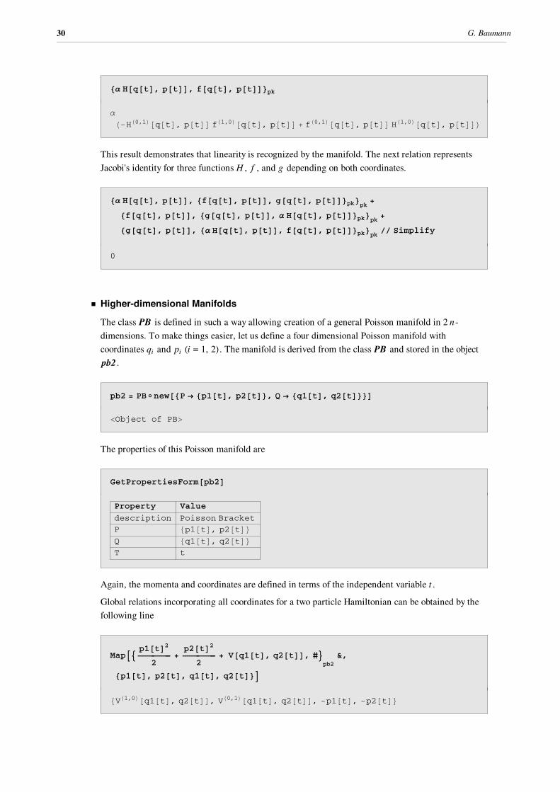
αH−HH0,1L@q@tD, p@tDD fH1,0L@q@tD, p@tDD + fH0,1L@q@tD, p@tDD HH1,0L@q@tD, p@tDDLThis result demonstrates that linearity is recognized by the manifold. The next relation represents

Jacobi's identity for three functions H , f , and g depending on both coordinates.

8α H@q@tD, p@tDD, 8f@q@tD, p@tDD, g@q@tD, p@tDD<pk<pk +

8f@q@tD, p@tDD, 8g@q@tD, p@tDD, α H@q@tD, p@tDD<pk<pk +

8g@q@tD, p@tDD, 8α H@q@tD, p@tDD, f@q@tD, p@tDD<pk<pk êê Simplify

0

ü Higher-dimensional Manifolds

The class PB is defined in such a way allowing creation of a general Poisson manifold in 2 n-

dimensions. To make things easier, let us define a four dimensional Poisson manifold with

coordinates qi and pi Hi = 1, 2L . The manifold is derived from the class PB and stored in the object

pb2 .

pb2 = PBÎnew@8P → 8p1@tD, p2@tD<, Q → 8q1@tD, q2@tD<<D

<Object of PB>

The properties of this Poisson manifold are

GetPropertiesForm@pb2D

Property Value

description Poisson BracketP 8p1@tD, p2@tD<Q 8q1@tD, q2@tD<T t

Again, the momenta and coordinates are defined in terms of the independent variable t .

Global relations incorporating all coordinates for a two particle Hamiltonian can be obtained by the

following line

MapA9p1@tD2

2+p2@tD2

2+ V@q1@tD, q2@tDD, #=

pb2&,

8p1@tD, p2@tD, q1@tD, q2@tD<E8VH1,0L@q1@tD, q2@tDD, VH0,1L@q1@tD, q2@tDD, −p1@tD, −p2@tD<

30 G. Baumann

The function used as the first argument of the PB is a Hamiltonian consisting of two terms for the

kinetic energy and a general interaction potential V . For another two dimensional Hamiltonian

with a different potential V we find

MapAi

kjjjj9

p1@tD2

2+p2@tD2

2+ V@q1@tDD, #=

pb2

y

{zzzz &, 8p1@tD, p2@tD, q1@tD, q2@tD<E

8V @q1@tDD, 0, −p1@tD, −p2@tD<The following example demonstrates that the Poisson bracket with two identical arguments, here a

Hamiltonian, vanishes

9p1@tD2

2+p2@tD2

2+ V@q1@tDD,

p1@tD2

2+p2@tD2

2+ V@q1@tDD=

pb2

0

So far, we defined the algebraic structure and derived certain types of Poisson manifolds by

specifying the phase space variables. However, the knowledge of these manifolds allows us to go a

step further to a real application and to introduce Hamilton's equations. Knowing the Poisson

manifold, it is straight forward to write down these equations.

Definition of Hamilton's Equations

For a set of generalized coordinates Hqk , pkL , Hamilton's equations are defined by

(20)q° k = ∑HÅÅÅÅÅÅÅÅÅÅ∑ pk

(21)p° k = - ∑HÅÅÅÅÅÅÅÅÅ∑qk.

This set of equations are related to Poisson's bracket by considering a function f in the phase space

depending on the phase space coordinates qk , pk , and t as

(22)f = f H qk , pk , tL .

The structure of the phase space is governed by Poisson's bracket which can be seen by

differentiating f with respect to t

(23)dfÅÅÅÅÅÅdt = ∑ fÅÅÅÅÅÅÅ∑t + ‚k=1

r ∑ fÅÅÅÅÅÅÅÅÅ∑qkq° k + ∑ fÅÅÅÅÅÅÅÅÅ∑pk

p° k .

By inserting Hamilton's equations of motion into this expression we gain

(24)dfÅÅÅÅÅÅdt = ∑ fÅÅÅÅÅÅÅ∑t + ‚k=1

r ∑ fÅÅÅÅÅÅÅÅÅ∑qk

∑HÅÅÅÅÅÅÅÅÅ∑pk- ∑ fÅÅÅÅÅÅÅÅÅ∑pk

∑HÅÅÅÅÅÅÅÅÅ∑qk.

Let us abbreviate by

(25)‚k=1

r ∑ fÅÅÅÅÅÅÅÅÅ∑qk

∑HÅÅÅÅÅÅÅÅÅ∑pk- ∑ fÅÅÅÅÅÅÅÅÅ∑pk

∑HÅÅÅÅÅÅÅÅÅ∑qk= 8 f , H<8q,p<

Elements

the Poisson's bracket defined on the phase space spanned by the coordinates qk and pk . The

subscript 8q, p< denotes the set of variables of the phase space. Using this definition, the temporal

change of f becomes

(26)dfÅÅÅÅÅÅdt = ∑ fÅÅÅÅÅÅÅ∑t + 8 f , H<8q,p<.Note that this relation allows us to calculate the temporal changes of any function depending on the

phase space variables.

We already encountered conserved quantities which have the property that their temporal change

vanish. This vanishing can be expressed by the Poisson bracket in a very convenient way. The

conservation of the quantity f implies

(27)dfÅÅÅÅÅÅdt = 0

which is identical with

(28)∑ fÅÅÅÅÅÅÅ∑t + 8 f , H<8q,p< = 0.

The above relations define a connection between a Poisson manifold and a Hamilton system. Thus,

the two properties connected by the manifold are denoted as a Poisson-Hamilton (PH) manifold. The

equations of motion for any kind of function in this manifold can be derived by means of the Poisson

bracket via equation (26).

It is convenient here to define a class for Hamilton's equations which inherits the properties of the

Poisson bracket. The properties of the Poisson manifold are equivalent to the properties of the

Hamilton manifold.

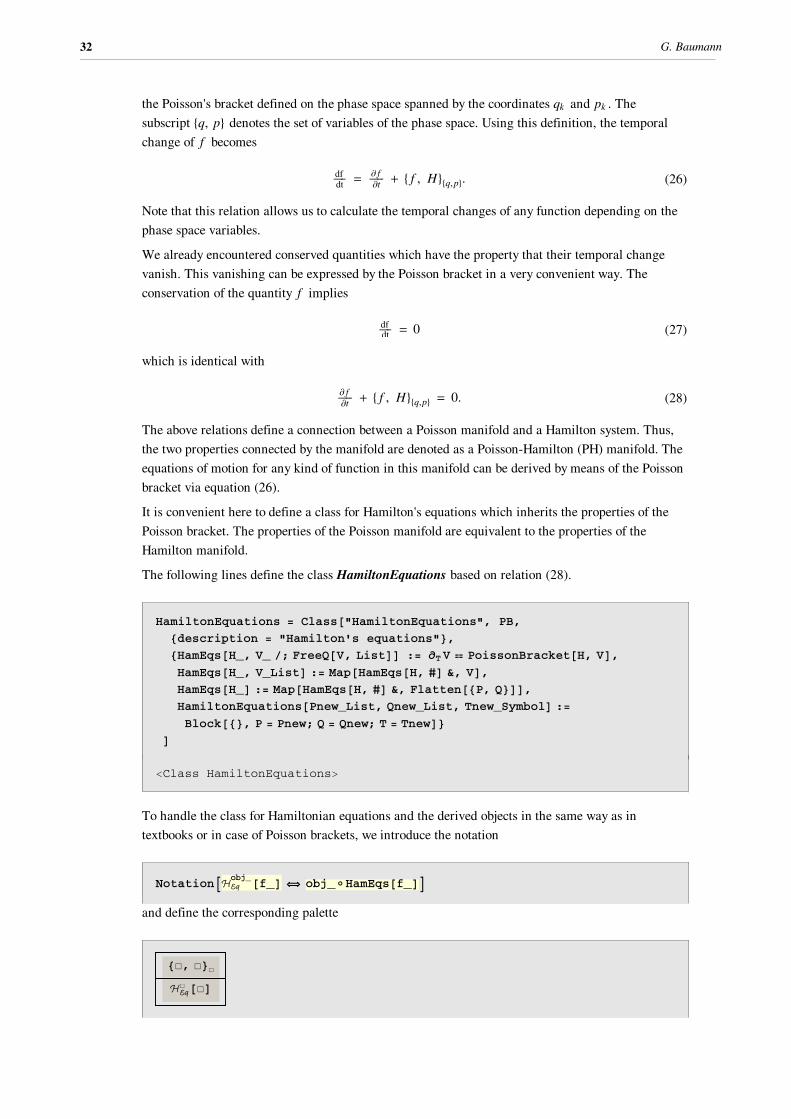
The following lines define the class HamiltonEquations based on relation (28).

HamiltonEquations = Class@"HamiltonEquations", PB,

8description = "Hamilton's equations"<,8HamEqs@H_, V_ ê; FreeQ@V, ListDD := ∂T V PoissonBracket@H, VD,HamEqs@H_, V_ListD := Map@HamEqs@H, #D &, VD,HamEqs@H_D := Map@HamEqs@H, #D &, Flatten@8P, Q<DD,HamiltonEquations@Pnew_List, Qnew_List, Tnew_SymbolD :=

Block@8<, P = Pnew; Q = Qnew; T = TnewD<D

<Class HamiltonEquations>

To handle the class for Hamiltonian equations and the derived objects in the same way as in

textbooks or in case of Poisson brackets, we introduce the notation

NotationAobj_@f_D obj_ÎHamEqs@f_DE

and define the corresponding palette

8 , <

@ D

32 G. Baumann

Having these tools available, we can apply the classes to specific problems.

ü Hamilton's Equations

As a first example let us examine a Hamilton-Poisson manifold with a single coordinate and a single

momentum. The object defining the Hamilton-Poisson manifold is created by

ham1 = HamiltonEquationsÎnew@8P → 8p@tD<, Q → 8q@tD<<D

<Object of HamiltonEquations>

Specifying a single particle Hamiltonian by kinetic and potential energies, we can derive the set of

Hamilton's equations by applying the manifold to the Hamiltonian.

ham1A

p@tD2

2+ V@q@tDDE

8p @tD == V @q@tDD, q @tD == −p@tD<The result is a system of equations defining the dynamic motion of this particle.

A second example is concerned with a four dimensional PH manifold. The generalized coordinates

and the momenta are primarily given by q1 , q2 , p1 and p2 .

ham2 = HamiltonEquationsÎnew@8P → 8p1@tD, p2@tD<, Q → 8q1@tD, q2@tD<<D

<Object of HamiltonEquations>

As an example, let us consider the double pendulum. The Hamiltonian for this system reads

HamDoublePendulum =1

2 l12 l2

2 m2 Hm1 + m2 Sin@θ1@tD − θ2@tDD2L

Hl22 m2 p1@tD2 + l12 Hm1 + m2L p2@tD2 − 2 m2 l1 l2 p1@tD p2@tD Cos@θ1@tD − θ2@tDDL −

m2 g l2 Cos@θ2@tDD − Hm1 + m2L g l1 Cos@θ1@tDD

−g Cos@θ2@tDD l2 m2 − g Cos@θ1@tDD l1 Hm1 + m2L +Hl22 m2 p1@tD2 − 2 Cos@θ1@tD − θ2@tDD l1 l2 m2 p1@tD p2@tD + l12 Hm1 + m2L p2@tD2L êH2 l12 l22 m2 Hm1 + Sin@θ1@tD − θ2@tDD2 m2LL

where pi Hi = 1, 2L are the generalized momenta, li , mi are the inertia momenta and the masses of

the particles and qi are the angles of deviation. This Hamiltonian is described in Eric Weinstein's

World of Science and can be found at

http://scienceworld.wolfram.com/physics/DoublePendulum.html. The PH manifold ham2 defined

above does not exactly correspond to the variables used in the Hamiltonian. However, we are able to

change the coordinate names by setting the properties of the PH manifold using

SetProperties@ ham2, 8P → 8p1@tD, p2@tD<, Q → 8θ1@tD, θ2@tD<<D

Elements

Now the PH manifold is defined for the coordinates

GetPropertiesForm@ham2D

Property Value

description Hamilton' s equationsP 8p1@tD, p2@tD<Q 8θ1@tD, θ2@tD<T t

The four equations of motion can then be gained by

equationsOfMotion = ham2@HamDoublePendulumD9p1 @tD == g Sin@θ1@tDD l1 Hm1 + m2L +

1

2 l12 l2

2 m2 ikjj 2 Sin@θ1@tD − θ2@tDD l1 l2 m2 p1@tD p2@tD

m1 + Sin@θ1@tD − θ2@tDD2 m2 −H2 Cos@θ1@tD − θ2@tDD Sin@θ1@tD − θ2@tDD m2 Hl22 m2 p1@tD2 −

2 Cos@θ1@tD − θ2@tDD l1 l2 m2 p1@tD p2@tD + l12 Hm1 + m2L p2@tD2LL íHm1 + Sin@θ1@tD − θ2@tDD2 m2L2y{zz, p2 @tD == g Sin@θ2@tDD l2 m2 +

1

2 l12 l2

2 m2 ikjj−

2 Sin@θ1@tD − θ2@tDD l1 l2 m2 p1@tD p2@tDm1 + Sin@θ1@tD − θ2@tDD2 m2 +H2 Cos@θ1@tD − θ2@tDD Sin@θ1@tD − θ2@tDD m2Hl22 m2 p1@tD2 − 2 Cos@θ1@tD − θ2@tDD l1 l2 m2 p1@tD p2@tD +

l12 Hm1 + m2L p2@tD2LL í Hm1 + Sin@θ1@tD − θ2@tDD2 m2L2y{zz,

θ1 @tD ==−2 l2

2 m2 p1@tD + 2 Cos@θ1@tD − θ2@tDD l1 l2 m2 p2@tD2 l1

2 l22 m2 Hm1 + Sin@θ1@tD − θ2@tDD2 m2L ,

θ2 @tD ==

2 Cos@θ1@tD − θ2@tDD l1 l2 m2 p1@tD − 2 l12 Hm1 + m2L p2@tD

2 l12 l2

2 m2 Hm1 + Sin@θ1@tD − θ2@tDD2 m2L =They represent the dynamics of the double pendulum in the Poisson-Hamilton manifold. This

example demonstrates the fact that using an object oriented approach the knowledge of the

Hamiltonian and the coordinates for the manifold suffices to derive the equations of motion in a

portion of a second. The ease of use and the close connection to textbook presentations allows for a

fast manipulation and reliable calculation of results. Beside of these examples, many other

applications of Elements to similar subjects are ahead.

34 G. Baumann

à ConclusionsIn this paper we discussed basic guidelines for building a sophisticated object oriented modeling

environment based on a knowledge base containing predefined components. We presented the

package Elements that implements the core functionality of such a system that is suitable to be used

for both industrial and mathematical applications. We demonstrated that combining the

computational power of computer algebra with object oriented paradigms provides a firm foundation

for speeding up the work flow in industrial modeling processes. The soundness and consistency of

the stored information ensures its practical applicability in a variety of settings.

à References[1] Paul~F.Dubois. Object technology for scientific computing. Prentice Hall, 1996.

[2] Kevin Dowd. High Performance Computing. O'Reilly & Associates, Inc., 1993.

[3] Guido Buzzi-Ferraris. Scientific {C++}:Building numerical libraries the object-oriented way.Addison-Wesley,1993.

[4] Daoqi Yang. C++ and Object Oriented Numeric Computing for Scientists and Engineers. Springer-Verlag, 2000.

[5] Matthias Berth, Frank-Michael Moser, and Arrigo Triulzi. Implementing computational services based on OpenMath.

In Ganzha et~al., pages 49-60.

[6] Manfred Göbel, Wolfgang Küchlin, Stefan Müller, and Andreas Weber. Extending a Java based framework for

scientific software-components. In V.G.Ganzha, E.W.Mayr, and E.V.Vorozhtsov, editors, Computer Algebra in

Scientific Computing,CASC'99. Proceedings of the Second International Workshop on Computer Algebra in Scientific

Computing, Munich, pages 207-222. Springer-Verlag, May 1999.

[7] Modelica Association. Modelica - a unified object oriented language for physical systems modeling.language

specification version 2.0. Modelica Association, http://www.modelica.org/, February 2002.

[8] Peter Fritzson, Johan Gunnarson, and Mats Jirstrand. MathModelica: an extensible modeling and simulation

environment with integrated graphics and literate programming. In Martin Otter, editor, The proceedings of the 2nd

International Modelica Conference, Oberpfaffenhofen, Germany, pages 41-54. DLR, Oberpffafenhofen, Germany,

March 2002.

[9] Victor G. Ganzha, Dmytro Chibisov, and Evgenii V. Vorozhtsov. GROOME - tool supported graphical object oriented

modeling for computer algebra and scientific computing. In V.G.Ganzha, E.W.Mayr, and E.V.Vorozhtsov, editors,

Computer Algebra in Scientific Computing, CASC 2001. Proceedings of the Fourth International Workshop on

Computer Algebra in Scientific Computing, Konstanz, pages 213-232. Springer-Verlag, July 2001.

[10] Roman Maeder. The Mathematica Programmer. AP Professional,1994.

[11] Michal Mnuk and Gerd Baumann. Elements. In V.G.Ganzha, E.W.Mayr, and E.V.Vorozhtsov, editors, Computer

Algebra in Scientific Computing, CASC 2002. Proceedings of the Fifth International Workshop on Computer Algebra in

Scientific Computing, Yalta, Ukraine, pages 227-236. Technische Universität München, Garching, September 2002.

[12] Andreas Weber, Gabor Simon, Wolfgang Küchlin, and Jörg Hoss. Lessons learned from using CORBA for

components in scientific computing. In Ganzha et~al., pages 409-422.

V.G.Ganzha, E.W.Mayr, and E.V.Vorozhtsov, editors. Computer Algebra in Scientific Computing, CASC 2000.

Proceedings of the Third International Workshop on Computer Algebra in Scientific Computing, Samarkand. Springer-

Verlag, October 2000.

Elements

About the Authors

Gerd Baumann is associated with the faculty of Physics at the University of Ulm. He is the author of

the books Mathematica in Theoretical Physics, and Symmetry Analysis of Differential Equations

with Mathematica. He is professor at the University of Ulm.

Michal Mnuk is associated with the faculty of Informatics at the Technical University of Munich.

He holds a Ph.D. degree in mathematics from the Research Institute for Symbolic Computation,

Hagenberg, and is currently on the way to finish his Habilitation at the Technical University of

Munich.

36 G. Baumann