elevation over azimuth position controller over azimuth position controller prepared by: thomas...
TRANSCRIPT


Elevation over Azimuth Position Controller
Prepared by:
Thomas Davies
Fourth-Year Electrical Engineering Student
University of Cape Town
19th October 2004
File: Thesis.lyx
Document No: 4028
Document Rev: A

Declaration
I declare that this project report is my own, unaided work. Itis a project report submitted
to the Department of Electrical Engineering, University ofCape Town, in partial fulfil-
ment of the requirements for the degree of Bachelor of Science in Engineering. It has not
been submitted before for any degree or examination in any other university.
Signature of Author . . . . . . . . . . . . . . . . . . . . . . . . . . . . . . . . . .. . . . . . . . . . . . . . . . . . . . . . . . . . . .
Cape Town 19th October 2004
i

Abstract
This project concerns the design and implementation of an elevation over azimuth position
controller for a Navy Jammer pedestal. The position controller system is implemented on
a Cogent CSB337 Single Board Computer using position resolvers to provide position in-
formation. The position controller accepts digital position commands moves the pedestal
to the appropriate position.
ii

Acknowledgements
I would like to thank Simon Winberg, Georgie Georgie and the rest of the Radar Remote
Sensing Group for helping me throughout this project. I would also like to thank Kevin
Stout, Bodo Sieber and Simon Lukell for their support throught this project period.
Finally I would like to thank Professor Inggs from the University of Cape Town for his
supervision and guidance during this project.
iii

Contents
Declaration i
Abstract ii
Acknowledgements iii
List of Symbols xi
Nomenclature xii
1 Introduction 1
1.1 Subject of this report . . . . . . . . . . . . . . . . . . . . . . . . . . . . 1
1.2 Background to Study . . . . . . . . . . . . . . . . . . . . . . . . . . . . 2
1.3 Objectives . . . . . . . . . . . . . . . . . . . . . . . . . . . . . . . . . . 2
1.3.1 Examination of the Pedestal Hardware and Interface Design . . . 2
1.3.2 Selection of a Platform for the Digital Control System. . . . . . 3
1.3.3 Designing and coding the software . . . . . . . . . . . . . . . . .3
1.3.4 Interfacing the hardware to the software . . . . . . . . . . .. . . 4
1.3.5 Evaluating System Response and Deriving a Control System . . . 4
1.3.6 Overall Testing . . . . . . . . . . . . . . . . . . . . . . . . . . . 4
1.4 Limitations and Scope . . . . . . . . . . . . . . . . . . . . . . . . . . . 4
1.5 Plan of Development . . . . . . . . . . . . . . . . . . . . . . . . . . . . 4
2 Position Control Concept Overview 6
iv
3 Background to the Hardware on the pedestal 9
3.1 Synchro Control Transformers . . . . . . . . . . . . . . . . . . . . . .. 9
3.2 Position Resolver Transmitters . . . . . . . . . . . . . . . . . . . .. . . 10
3.2.1 Excitation of rotor windings . . . . . . . . . . . . . . . . . . . . 10
3.2.2 Excitation of stator windings . . . . . . . . . . . . . . . . . . . .12
3.2.3 Reference Frequency . . . . . . . . . . . . . . . . . . . . . . . . 13
3.3 Tachometric Generators . . . . . . . . . . . . . . . . . . . . . . . . . . .14
3.4 Direct Current Brushed Motors . . . . . . . . . . . . . . . . . . . . . .. 14
3.5 Brake . . . . . . . . . . . . . . . . . . . . . . . . . . . . . . . . . . . . 14
4 Interfacing with the hardware 15
4.1 Synchro Resolver . . . . . . . . . . . . . . . . . . . . . . . . . . . . . . 15
4.2 Position Resolver Conversion . . . . . . . . . . . . . . . . . . . . . .. . 16
4.2.1 Measuring Position Resolver Output Signals . . . . . . . .. . . 16
4.2.2 Input Reference Signal . . . . . . . . . . . . . . . . . . . . . . . 18
4.3 Movement of the Pedestal . . . . . . . . . . . . . . . . . . . . . . . . . . 19
4.3.1 Digital to Analogue Conversion . . . . . . . . . . . . . . . . . . 19
4.3.2 Motor Drive Circuit . . . . . . . . . . . . . . . . . . . . . . . . 20
4.3.3 Tachogenerator interface . . . . . . . . . . . . . . . . . . . . . . 20
5 Platform for the Position Controller Software 21
5.1 The CSB337 Single Board Computer . . . . . . . . . . . . . . . . . . . .21
5.1.1 Important Components on the CSB337 . . . . . . . . . . . . . . 21
5.1.2 The CSB300CF Break-out Board . . . . . . . . . . . . . . . . . 22
5.2 Running Software on the CSB337 . . . . . . . . . . . . . . . . . . . . . 22
5.2.1 Arm-Linux Toolchain . . . . . . . . . . . . . . . . . . . . . . . 23
5.2.2 Hello World Program . . . . . . . . . . . . . . . . . . . . . . . . 23
5.2.3 MicroMonitor . . . . . . . . . . . . . . . . . . . . . . . . . . . . 23
5.3 Embedded Operating System . . . . . . . . . . . . . . . . . . . . . . . . 23
v

6 Software to Control the System 25
6.1 Overall Design . . . . . . . . . . . . . . . . . . . . . . . . . . . . . . . 25
6.1.1 Data Flow of the Software . . . . . . . . . . . . . . . . . . . . . 25
6.2 Objects in the Position Controller Software . . . . . . . . . .. . . . . . 27
6.2.1 The Timer Class . . . . . . . . . . . . . . . . . . . . . . . . . . 27
6.2.2 The Pedestal Kernel Module . . . . . . . . . . . . . . . . . . . . 28
6.2.3 The Controller Class . . . . . . . . . . . . . . . . . . . . . . . . 28
6.3 Sequence of Events in the Position Controller Software .. . . . . . . . . 29
6.4 Software Testing . . . . . . . . . . . . . . . . . . . . . . . . . . . . . . 29
6.4.1 Pedestal Kernel Module . . . . . . . . . . . . . . . . . . . . . . 29
6.4.2 Timer Class . . . . . . . . . . . . . . . . . . . . . . . . . . . . . 32
6.4.3 Controller Class . . . . . . . . . . . . . . . . . . . . . . . . . . 32
7 Discussion of Results 33
7.1 Sampling Frequency of the ADC . . . . . . . . . . . . . . . . . . . . . . 33
7.2 Resolver Position Conversion . . . . . . . . . . . . . . . . . . . . . .. . 33
7.2.1 Power Supply to Analogue-to-Digital Converter Circuit . . . . . . 33
7.2.2 Analogue to Digital Conversion Accuracy . . . . . . . . . . .. . 34
7.3 Digital to Analogue Conversion Accuracy . . . . . . . . . . . . .. . . . 35
7.4 Overall Performance of Position Controller . . . . . . . . . .. . . . . . 37
8 Conclusions and Recommendations 38
8.1 Position Resolver Accuracy . . . . . . . . . . . . . . . . . . . . . . . .. 38
8.1.1 Recommendations for Improving Accuracy . . . . . . . . . . .. 38
8.2 Position Controller Performance . . . . . . . . . . . . . . . . . . .. . . 39
8.2.1 Recommendations for Improving Controller Performance . . . . 39
A Resolver Module 40
B Postioner Application 41
vi

Bibliography 42
vii
List of Figures
1.1 Navy EW Jamer Pedestal . . . . . . . . . . . . . . . . . . . . . . . . . . 1
2.1 Typical Position Control Loop System . . . . . . . . . . . . . . . .. . . 6
2.2 A Motor Rate Control System . . . . . . . . . . . . . . . . . . . . . . . 7
2.3 Position Controller Control Loop . . . . . . . . . . . . . . . . . . .. . . 7
3.1 Internal Design of Synchro Control Transformer . . . . . . .. . . . . . . 10
3.2 Internal Structure of a Resolver Transmitter . . . . . . . . .. . . . . . . 11
3.3 Output Signals of Position Resolver for Varying Shaft Angles . . . . . . . 12
3.4 Signals on Position Resolver with Stator Excitation . . .. . . . . . . . . 13
4.1 The Goertzel Algorithm as a Second Order Filter . . . . . . . .. . . . . 18
5.1 The Cogent CSB337 . . . . . . . . . . . . . . . . . . . . . . . . . . . . 21
5.2 Abstraction Layers of an Operating Systems . . . . . . . . . . .. . . . . 24
6.1 Data-flow Context Diagram of Position Controller . . . . . .. . . . . . . 26
6.2 Data-flow Level 1 Diagram of Position Controller . . . . . . .. . . . . . 26
6.3 Data-flow Diagram of Controller Class . . . . . . . . . . . . . . . .. . . 27
6.4 Class Diagram of Timer Class . . . . . . . . . . . . . . . . . . . . . . . 27
6.5 Class Diagram of Pedestal Driver Module . . . . . . . . . . . . . .. . . 28
6.6 Class Diagrams of Controller Class . . . . . . . . . . . . . . . . . .. . . 29
6.7 Flowchart of Position Controller Operation . . . . . . . . . .. . . . . . 30
6.8 UML Sequence Diagram for Position Controller . . . . . . . . .. . . . . 31
viii

7.1 ADCBUSY Signal . . . . . . . . . . . . . . . . . . . . . . . . . . . . . 34
7.2 Power Supply Noise . . . . . . . . . . . . . . . . . . . . . . . . . . . . . 34
7.3 ADC Output with Inputs at Ground . . . . . . . . . . . . . . . . . . . . .35
7.4 Position Output for Constant Angular Rate . . . . . . . . . . . .. . . . . 36
7.5 DAC Output for Different Input Codes . . . . . . . . . . . . . . . . .. . 36
7.6 Motor Rate for Position Command . . . . . . . . . . . . . . . . . . . . .37
ix

List of Tables
4.1 Relevant ADS7824 ADC Specifications . . . . . . . . . . . . . . . . .. 16
4.2 Motor Drive Command Conversions . . . . . . . . . . . . . . . . . . . .20
7.1 ADC Conversion Error . . . . . . . . . . . . . . . . . . . . . . . . . . . 35
7.2 DAC Performance . . . . . . . . . . . . . . . . . . . . . . . . . . . . . . 36
x

List of Symbols
θ — I
K — Motor gain
Tm — Mechanical time constant
E f — Field Voltage
ω — Reference signal frequency
ωsha f t — Shaft frequency
VR — Peak reference voltage
xi

Glossary
Azimuth—Angle in a horizontal plane, relative to a fixed reference, usually north or the
longitudinal reference axis of the aircraft or satellite.
Elevation—Angle in a vertical plane, relative to a fixed reference, usually the horizontal
plane.
Interrupt—An event that interrupts normal processing and temporarily diverts flow-of-
control through an interrupt service routine.
Pedestal—The structure which supports an antenna.
Rotor—The rotating armature of a motor or generator.
Selsyn—A system that consists of two or more motor-like devices that are intended to
sense or control shaft position.
Servo-motor—The area on earth covered by the antenna signal.
Stator—The stationary part of a motor or generator in or around which the rotor revolves.
Transducer—An electrical device that converts one form of energy into another.
xii

Chapter 1
Introduction
1.1 Subject of this report
This document concerns the design, implementation and testing of an elevation over az-
imuth position controller for a Navy electronic warfare (EW) jammer pedestal using a
single board computer (SBC). The requirement for this project is that the antenna on the
pedestal has to be moved by the position controller to a specific position or in a search
pattern as input to the SBC.
Figure 1.1: Navy EW Jamer Pedestal
1

1.2 Background to Study
The University of Cape Town has a Navy EW jammer pedestal for experimentation as
can be seen in figure 1.1. The pedestal has two axes of movement: the horizontal (or
azimuth axis), and the vertical (or elevation) axis. Since the elevation axis is closer to
the antenna than the azimuth axis, the pedestal is known as anelevation over azimuth
pedestal. The pedestal uses 28 volt direct current (DC) motors to move the antenna in
each axis. The position of each axis is measured using position resolvers, and the rate at
which the antenna is moving is measured using tachogenerators.
The requirement of this project is to create a controller that will move the antenna to
specific positions as input to the SBC. The movement has to be accurate, take as short
an amount of time as possible and the position has to be maintained without minimal
deviation.
1.3 Objectives
The objective of this project is to create a position controller with the equipment available
that will move the position of the antenna in a manner optimised for speed and accuracy.
The inputs are either of the following:
• Elevation and azimuth position
• Search pattern1
The position controller is based around a SBC, with the digital control algorithm imple-
mented in software.
The project was divided into the following tasks:
1.3.1 Examination of the Pedestal Hardware and Interface Design
The first task in this project was to examine the characteristics of the components already
on the pedestal and to test which of the components were stillfunctional. As most of the
documentation for the electronics on the pedestal is unavailable, electrical characteristics
of certain components had to be measured to derive specifications. Once a better under-
standing of all the equipment is gained, a mathematical model for the position control
process could be derived, and a hardware interface to the controller could be designed.
1Such asnodding or raster
2

Circuitry needed to be built which ensured that input signals and power supplies to the
various components did not exceed operating specifications. Output from the position
resolvers had to be converted from an analog signal to one which could be used by the
digital components of the position controller. The motors required circuits which drove
them at varying torque according to a reference signal. The rate information from the
tachogenerators had to be fed back into the motor drive circuit within an inner rate loop.
1.3.2 Selection of a Platform for the Digital Control System
A decision between a PC and a single board computer had to be made, and due to the real
time requirements a Cogent CSB337 single board computer wasused as the platform for
the position controller.
The CSB337 is a highly integrated SBC with a number of useful interfaces, devices and
software tools that make it suitable for embedded control applications. The hardware
devices include RS-232 Serial Ports for communication, Ethernet interface for network
connection and Inter Integrated Circuit (I2C) bus and serial peripheral interface (SPI)
for device connectivity. The SBC has 8 MBytes of SDRAM to store data and programs
in during operation and 32 MBytes of Flash memory for non-volatile storage of data or
programs.
The CSB337 has a bootloader (MicroMonitor) pre-installed to load software into memory
as it boots up and to initialise system registers.
A decision had to be made on whether to install an operating system on the SBC or
to write stand-alone software. It was decided that it would be best to install an operating
system and different types of operating systems where examined. A toolchain was created
to enable software and an operating to be compiled for the SBC.
The real time operating system that is used is SnapGear Linux, which is based on uClinux.
It can be run as a Real Time Operating System (RTOS) and comes with a number of pack-
ages. Applications and kernel modules were designed to testinterfaces and peripherals
on the single board computer.
1.3.3 Designing and coding the software
Universal Modelling Language (UML) class and data-flow diagrams were used to design
the software in a top-down approach. The highest level was broken down into smaller
pieces and described in UML. This process was repeated for each smaller section until
there were three layers of hierarchy. C and C++ headers were generated from the UML
class diagrams and the working code was generated based on the headers. The kernel
modules were written in C, and the position controller application written in C++.
3

1.3.4 Interfacing the hardware to the software
An interface was designed to integrate the hardware and software in a stable and coher-
ent manner. Tests were done to ensure the voltage levels werecorrect at the inputs and
outputs. Kernel modules were tested to ensure that the circuits work correctly, and the
actual response of each component was compared to the desired response. Designs were
modified and adjusted to optimise performance and the expected error in each device was
calculated and then measured.
1.3.5 Evaluating System Response and Deriving a Control System
With all the circuits and components functioning correctlythe response of the system was
measured and the parameters of the mathematical model for the system were calculated.
The mathematical model described the manner in which the inputs affect the systems
output and was used to design a controller. The controller was then implemented.
1.3.6 Overall Testing
Although testing was done at the end of each the tasks where possible, the overall system
was tested and the results recorded and interpreted. Position commands were input to the
system and the time and accuracy of the response was measured. The overall system was
found to have an accuracy of 42 arc minutes.
1.4 Limitations and Scope
The focus of this report is not to create the best possible design for a position controller,
but to create an accurate and efficient controller with the equipment at hand.
This project covers many different areas, including; hardware design, analog and digital
interfacing, real time operating systems and embedded application programming. Due to
the time constraints, not all areas could be examined in great detail, and would benefit
from more exploration in the future.
1.5 Plan of Development
Chapter 2 gives a conceptual overview of the position controller system.
Chapter 3 is a background to the hardware on the pedestal.
4

Chapter 4 describes the interface to the hardware on the pedestal
Chapter 5 is a description of the software
Chapter 6 discusses the results obtained from the system
Chapter 7 makes conclusions based on those results and givesrecommendations based on
those conclusions
5

Chapter 2
Position Control Concept Overview
The method of controlling position is a closed loop control system as represented in fig-
ure 2.1. A sensor provides information about the current state of the process and a com-
parator compares the measured state to the desired state andoutputs an error signal. A
controller produces a driving output based on this error signal.
MotorCommand Error
Sensor
Position+
-Controller
E�f�
Measured Position
Figure 2.1: Typical Position Control Loop System
In the position controller system on the navy pedestals there is feedback information about
the current motor rate provide, therefore a rate loop can be installed on the system as in
figure 2.2.
The digital position control loop would then be closed around this rate loop and the overall
position controller is shown in figure 2.3
The overall transfer function of a position control of this type has the form of equation 2.1,
[22].
G(s) =K
s(s+α)(2.1)
6

Integral
Proportional
Tachogenerator
Motor+
-
+
+Command
ErrorOutput
Figure 2.2: A Motor Rate Control System
Rate Loop& Motor
+Command
ErrorResolverIntegral
Proportional
Position+
-
ADC
DAC+
Software Interface Hardware
Figure 2.3: Position Controller Control Loop
7

The parameters of this model will be calculated by the methods described in [17] and [23].
8

Chapter 3
Background to the Hardware on the
pedestal
This chapter is a description of the hardware components on the pedestal that relevant to
this project. The concepts involved in the components are described in detail where ap-
plicable, along with the methods of operation. Each component is described individually.
3.1 Synchro Control Transformers
A synchro control transformer (CT) is a form of angular transducer. CTs are rotating
transformers that output an analogue voltage that is uniquely related to the input shaft
angle. A CT consists of a rotor with one winding which revolves around a stator with
3 windings in wye format, 120 degrees apart. The internal wiring is demonstrated in
figure 3.1.
A CT accepts input voltage across the stator terminals as desribed in equation 3.1 [20, 15,
6].
S1–S3= sinωt sinθ
S3–S2= sinωt sin(θ+120o)
S2–S1= sinωt sin(θ+240o) (3.1)
The rotor windings will then only produce a voltage across their terminals if the shaft
input on the CT is not at angleθ. This output voltage is an error signal which can be fed
into a phase sensitive detector and an error amplifier to produce a signal that will drive a
motor to the correct position, and thus provide a servo control system.
9

Figure 3.1: Internal Design of Synchro Control Transformer
3.2 Position Resolver Transmitters
Position resolver transmitters (TX) are angular transducers similiar in design to synchro
control transformers in that they consists of rotor which rotates inside a stator. A TX
outputs an analogue voltage that is uniquely related to its input shaft angle [9], just as a
synchro control transformer does. A TX however has two rotorwindings at 90 degrees
angle to each other and two stator windings also seperated bya 90 degree angle. The
internal wiring of a TX is shown in figure 3.2.
There are two common methods to calculate the shaft angle using position resolvers:
3.2.1 Excitation of rotor windings
If an alternating current is introduced across one of the rotor windings, a voltage is in-
duced in the stator windings. Since the stator windings are at right angles to each other,
the amplitudes of the voltages induced are related by the sine of cosine of the shaft an-
gle [20, 15]. If the stator windings are excited with a signal:
Asinωt (3.2)
The output of the stator windings will be:
S1–S3:Vx = VR sinωt sinθ
10

Figure 3.2: Internal Structure of a Resolver Transmitter
11

S2–S4:Vy = VR sinωt cosθ (3.3)
Therefore, according to [15] the shaft angleθ can be determined by:
θ = arctanVx
Vy(3.4)
The output of a CT is shown in figure 3.3
0 5 10 15−1
−0.5
0
0.5
1
Voltage
Tim
e
Stator Winding S1 to S3
0 5 10 15−1
−0.5
0
0.5
1
Voltage
Tim
e
Stator Winding S2 to S4
(a) Shaft at 0 degrees
0 5 10 15−1
−0.5
0
0.5
1
Voltage
Tim
e
Stator Winding S1 to S3
0 5 10 15−1
−0.5
0
0.5
1
Voltage
Tim
e
Stator Winding S2 to S4
(b) Shaft at 90 degrees
0 5 10 15−1
−0.5
0
0.5
1
Voltage
Tim
e
Stator Winding S1 to S3
0 5 10 15−1
−0.5
0
0.5
1
Voltage
Tim
e
Stator Winding S2 to S4
(c) Shaft at 180 degrees
0 5 10 15−1
−0.5
0
0.5
1
Voltage
Tim
e
Stator Winding S1 to S3
0 5 10 15−1
−0.5
0
0.5
1
Voltage
Tim
e
Stator Winding S2 to S4
(d) Shaft at 270 degrees
Figure 3.3: Output Signals of Position Resolver for VaryingShaft Angles
3.2.2 Excitation of stator windings
By exciting the two stator windings with two signals in phasequadrature to one another,
the voltage induced on the rotor winding will have a fixed amplitude and frequency, but
will have a phase that varies according to shaft angleθ [20, 9]. The input signals will be:
12

VS1−−S3 = VR sinωt
VS2−−S4 = VR sin(ωt +90o) = V cosωt (3.5)
The voltage induced across the rotor winding will be:
VR1−−R2 = VR sin(ωt +θ) (3.6)
The phase of the signal across the rotor winding will range from 0oto 360owhen com-
pared to the reference signal and can be measured to determine the shaft angle.
0 5 10 15−1
−0.8
−0.6
−0.4
−0.2
0
0.2
0.4
0.6
0.8
1S1−S3R1−R3S2−S4
ShaftAngle θ
Figure 3.4: Signals on Position Resolver with Stator Excitation
3.2.3 Reference Frequency
The output of the resolver with a rotating shaft will be a modulated carrier signal of the
form:
Vout put = sin(ωsha f tt)VR sin(ωt) (3.7)
In order to ensure that the correct angular information is conveyed, the reference fre-
quency must always be greater than the shaft rotational frequency [9].
13

3.3 Tachometric Generators
Tachometric generators (tachogenerators) are transducers which convert rotational veloc-
ity into voltage. The tachogenerators used in this project were Servo - Tek SA - 740A -2
and provided an output of 7 Volts (V) for every 1000 revolutions per minute (RPM).
3.4 Direct Current Brushed Motors
The pedestal is moved by two direct current (DC) brushed motors that operate from -28 V
to 28 V. The model type is Vactric 15P203, which has a maximum current rating of 0.95
Amps. The maximum rated speed is 5000 revolutions per minute(RPM) with a torque of
220 grams per centimeter.
3.5 Brake
There is a brake on the elevation axis to prevent uncontrolled movement in the system.
The brake is disengaged when a voltage greater than 24 V is applied.
14

Chapter 4
Interfacing with the hardware
This chapter examines the methods used in interfacing to thecomponents on the pedestal
in detail, describing the specifications of the components and the associated interface.
Calculations are made to determine optimal parameters for the interface and methods of
improving accuracy are explored where relevant.
4.1 Synchro Resolver
The original design for this particular pedestal was an analogue position controller that
made use of synchro control transformers and synchro control transmitters. In the original
design the desired position was set by means of a synchro control transmitter and the
synchro control transfomer provided feedback informationbased on the position of the
shaft.
The synchro control transformers on this pedestal require three phases of 115 V from line
to line at 400 Hertz (Hz) as an input to operate. The phases must be generated as described
in equation 3.1. The output of the synchro control transformer is an alternating signal 90
V root-mean-squared (RMS).
Navy and Airforce craft commonly use 400 Hz power supplies since 400 Hz generators
tend to be smaller and more efficient than more common 50 Hz generators [6]. However a
400 Hz power supply is not a common type of power supply and at the time of this project
only one 400 Hz generator was available at the University of Cape Town which was still
being tested.
A second disadvantage of using synchro resolvers is that with the high voltages required
for operation, integration with digital equipment is difficult and requires special hardware,
which is expensive. It was decided that since position resolvers can provide similar or im-
proved accuracy [20], the synchro control transformers would not be used in this project,
and be replaced by position resolvers on the pedestal .
15

4.2 Position Resolver Conversion
The position resolver output is in the form of two alternating signals described in equa-
tion 3.3. To calculate the shaft angleθfrom this output, the amplitudes of the two signals
need to be calculated. Since the shaft angle is related to theratio of these two amplitudes
(equation 3.4), either the peak value or the root-mean-squared (RMS) value can be used
to determine it.
4.2.1 Measuring Position Resolver Output Signals
Two analogue-to-digital converters ADCs were used in orderto measure the different
output signals simultaneously. The ADCs used in this project are Texas Instruments
ADS7824 CMOS 12 bit ADCs. The relevant characteristics are shown in table 4.1.
Table 4.1: Relevant ADS7824 ADC Specifications
Parameter Specification
Resolution 12 bitsMaximum Sampling Frequency 40kHz
DC Accuracy 1 LSBAnalogue Input Range -10 V to 10V
No. of Channels 4Data Output Coding Two’s Complement
Since the 12bit ADCs operate from -10V to 10V, the least signicant bit (LSB) corresponds
to:
20212−1
= 0.00489V= 4,89mV (4.1)
The ADC has no internal provision for correcting the internal bipolar zero error, but is
guaranteed to be below a level slightly more than two LSBs. The specifications guarantee
that the error between channels will be less than one LSB, andsince the measurement
required is a ratio of two channels, the zero offset error canbe ignored. Therefore the
error in calculating the ratio of two voltages will be a maximum of one LSB or 4,89 mV.
According to the specifications in table 4.1, the DC error is LSB, when added to the error
between channels the maximum total error becomes:
eadc = 2LSB= 9.78 mV (4.2)
The circuit used for the ADCs makes use of the Texas Instruments TAG feature [10],
16

which allows two ADCs to share input and output signals to minimise the use of data
lines.
Precautions need to be taken to avoid noise on the ADC circuitand the following methods
of eliminating noise were investigated:
Grounding Planes
Noise from digital signals causes large amounts of interference with the analogue-to-
digital conversion process [1]. To avoid this the analogue and digital grounding planes
were seperated and a decoupling capacitor was introduced between them.
Analogue Filtering
A possible method for removing noise is the introduction of an analogue filter before the
input to the ADCs. However, an analogue filter implemented here can be implemented
as a digital filter after the conversion process, without anyheat sensitivity or non-linear
response associated with some analogue devices [21].
Averaging of Samples
One of the most common methods for noise reduction is the averaging of a number of
samples [1]. This is effectively a low-pass filter and every time the number of samples is
doubled there is a reduction in noise by a factor of the squareroot of two.
The Goertzel Algorithm
The output signals from the position resolver are alternating signals at the same frequency
as the reference signal in equation 3.2. Therefore all otherfrequency components are
irrelevant and can be ignored. Since the only valuable information in those signals is
the amplitude of the signals at the reference frequency, a possible solution would be to
calculate the Discrete Fourier Transform (DFT) of those signals and examine the co-
efficients of that frequency.
To calculate the DFT the Goertzel algorithm is used because it is more efficient that the
fast Fourier Transform (FFT) when log2N co-efficients are required [12], and in this case
only one co-efficient is required.
The Goertzel algorithm is a Infinite Impulse Response (IIR) filter which is defined by
equation 4.3. It is implemented in the form of a second order filter as shown in figure 4.1
17

H (z) =1−W k
Nz−1
1−((
W kN −W−k
N
)
z−1+ z−2) (4.3)
k
Z -1
Z -1
2cos(w )k -WN
x(n) y(n)
Figure 4.1: The Goertzel Algorithm as a Second Order Filter
The effect of the Goertzel algorithm is that of a very high Q-factor band-pass filter which
removes most of the noise from the ADC input.
4.2.2 Input Reference Signal
The position resolvers on the pedestal are rated to accept analternating current (AC) input
of up to 10 Volts at 10 kHz. The full input voltage range is usedto minimise noise. This
range also allows the ADCs to be operated across their full range, without any need for
voltage conversion.
The reference frequency,fre f , to be used had to be less than the maximum rated frequency
and was determined by two criteria, namely:
1. The maximum sampling rate of the ADC circuit.
2. The maximum shaft rotation speed on the pedestal.
The maximum sampling frequency,fs, of the ADC circuit was conservatively estimated at
at 20kHz based on specifications, and later measured at 17,54kHz in chapter 7. According
to the Nyqist-Shanon sampling theorem [19, 21], the reference frequency has to be:
18

2 fre f < fs (4.4)
Therefore the reference frequency must be less than 8.770 kHz.
The maximum shaft rotation was tested by measuring the number of rotations per minute
that the pedestal could acheive when driven at full rate. This was found to be 14.83
revolutions per minute. Therefore the maximum shaft rotation frequency is:
2π(14.83)60= 5591.96 rad.sec−1 (4.5)
According to equation 3.7, this would require the referencefrequency be greater than
5591.96 rad.sec-1or 889.8 Hz.
This result meant that the reference frequency had to lie within the following range:
889.8≤ fre f ≤ 8770 Hz (4.6)
With higher frequencies more succeptable to noise interference, it was decided to use a
reference frequency of 1kHz.
A standard function Hewlett Packard 33120A function generator is used to generate the
reference frequency for the position resolvers.
4.3 Movement of the Pedestal
The position controller has an digital rate command that needs to converted into an ana-
logue current to the motor. The digital signal is converted by two digital-to-analogue
converters, one for each axis.
4.3.1 Digital to Analogue Conversion
The DACs used in this project are Texas Instruments 12bit TLV5616 Digital to Analogue
Converters. The DACs have an output range from 0 V to 2Vre f , whereVre f can be from 0 V
to 3.5 V. In this projectVre f is set at 3 V to avoid saturating the DAC in case of fluctuating
voltage supplies, while still provide a good voltage range.Therefore the output range of
the DAC is in the range of 0 V to 6 V.
19

4.3.2 Motor Drive Circuit
To move the pedestal the primary movers need to be supplied with a voltage in the range of
-28V to 28V depending on the desired movement rate and direction required. The motor
drive circuit used is provided by 4-Sight Optronics, based on a ST Microelectronics L292
Switch-Mode Driver, and accepts an input of the range -15V to15V, which corresponds
to an output to a motor in the range of -28 V to 28 V.
However, the input to the drive circuit is a unipolar DC voltage from the DACs in the
range of 0 to 6 Volts. Therefore this voltage needs to be offset and amplified so the input
to the motor drive circuit reflects the ranges described in table 4.2. This can be acheived
by equation 4.7 and is implemented by means of a classic differential amplifier [11] with
a gain of 5.
Vout = 5(Vin −3) (4.7)
Table 4.2: Motor Drive Command Conversions
Output from DAC Input to Motor Driver Circuit Input to Motor
0 V to 3 V -15 to 0V -28 to 0V3V 0 V 0 V
3 V to 6 V 0 V to 15V 0 V to 28 V
4.3.3 Tachogenerator interface
The rate information provided by the tachogenerator is connected through a voltage buffer
to the motor drive circuit. This provides feedback for the inner rate loop, and is added to
the error signal before the PI process of the position controller.
20

Chapter 5
Platform for the Position Controller
Software
This chapter describes the digital portion of the position controller, in particular the plat-
form on which the software will be run. The embedded device used for this project is
described, along with the method used in running software onit. A simple application is
then used to test the software creation process. The operating system used for this project
is then described.
5.1 The CSB337 Single Board Computer
The University of Cape Town has recently purchased a number of Cogent CSB337 Single
Board Computers (SBC) and one of which was made available foruse in this project.
The CSB337 is manufactured by Cogent Computer Systems, Inc.and is centered around
an ARM920T Core, namely the Atmel AT91RM9200 microprocessor. The CSB337 has
many highly integrated components on-board and the features applicable to this project
are examined in further detail as follows:
Figure 5.1: The Cogent CSB337
5.1.1 Important Components on the CSB337
RS-232 Serial Port
Basic communication is provided between the SBC and other data terminal equipment
(DTE), such as a PC, through this serial port. As the SBC is started the first RS-232 serial
port (uart 0) is monitored for communication by the bootloader software, MicroMonitor.
MicroMonitor provides basic control over the SDC through this serial port.
21

32 M-byte S-DRAM
The SBC has provide sufficient memory to load user programs orother data into on
startup. This memory is volatile and the contents is lost when the power is disconnected.
8 M-byte Strata FLASH
Non-volatile storage space is provide to store software or in absence of power. This
memory also holds the startup file,monrc, which can be configured to perform certain
tasks on startup.
Ethernet Interface
A 10/100 M-Bit Ethernet interface is provided via internal Media Access Control (MAC).
This allows connections to networks and fast transfer of data to and from the SBC.
5.1.2 The CSB300CF Break-out Board
The break-out board provides the following connectors for the CSB337.
• An Ethernet RJ45 connector for connecting to 10/100 Ethernet.
• DB9 connector for RS-232
• 5 Volt DC power connector
5.2 Running Software on the CSB337
Software can be written directly for the CSB337 in a variety of different programming
languages. The software for this project is written in C and C++, cross-compiled on a
Linux machine for a ARM processor.
To cross-compile for ARM, a toolchain is required to compileand link the C/C++ code
into an executable that can run on a ARM machine. The toolchain used in this project is
described in section 5.2.1.
22

5.2.1 Arm-Linux Toolchain
A precompiled uClinux arm-linux toolchain1 was used to compile applications directly
for the CSB337. The toolchain installed and compiled application for the ARM machine
without any significant problems.
5.2.2 Hello World Program
To test the CSB337 and thearm-linux toolchain, a simplehello world application2 was
compiled using the toolchain. The Gnu Complier Collection (gcc) version information
was:
gcc version 2.95.3 20010315 (release)(ColdFire patches - 20010318 from
http://fiddes.net/coldfire/)(uClinux XIP and shared lib patches from http://www.snapgear.com/)
Once thehello world application had been cross-compiled and linked it had to be copied
to SBC, this is acheived by usingMicroMonitor
5.2.3 MicroMonitor
A null modem cable connected to the SBC’suart0 RS-232 serial port provides basic
communication to a PC or other DTE. Using a terminal interface program calledminicom
and communicating with the parameters described in [2], basic communication with the
SBC using MicroMonitor was possible.
Thehello world application was transfered into the SBC’s Strata Flash using Trivial File
Transfer Protocol (TFTP) via the Ethernet interface. The application was then executed
and the returned succesfully.
5.3 Embedded Operating System
SnapGear Linux is used as an embedded operating system (EOS)on the SBC. The SnapGear
distribution of Linux is based on uClinux and comes with a variety of packages. The ver-
sion used in this project was compiled with the GNU C library (glibc).
The main reason for using an EOS in this project is the layer ofabstraction it provides
between the position controller software and the underlying system hardware. This is
shown in figure 5.2.
1Downloaded from http://www.snapgear.orghttp://www.snapgear.org2provided by Simon Winberg
23

Figure 5.2: Abstraction Layers of an Operating Systems
Linux is not a real-time operating system but provides performance which is acceptable
to soft real-time systems [16], such as a position controller.
24

Chapter 6
Software to Control the System
This chapter describes the overall design of the software used in the position controller,
beginning with the flow of data through the software. The different objects in the software
are then described in the Unified Modeling Language as in [14]. Sequence and flow in-
formation about the software is presented in the form of a flowchart and a UML sequence
diagram. Finally the methods used in testing the software are introduced.
6.1 Overall Design
6.1.1 Data Flow of the Software
Figure 6.1 is a data-flow diagram which demonstrates the basic interaction of the user,
the software and the hardware. The diagram consists of the external entities; the pedestal
interface, and the interface on the client machine and the main process; the position con-
troller. The client machine presents the position controller with a request for a new po-
sition, and the position controller process ensures that the motor is given the correct rate
information to drive the pedestal to the desired position.
Figure 6.2 demonstrates how the position controller software is broken down into smaller
processes and data storage points, and the internal data flowis demonstrated. There are
three main processes at this level which interact with one another through data stores, to
ensure that they are weakly coupled.
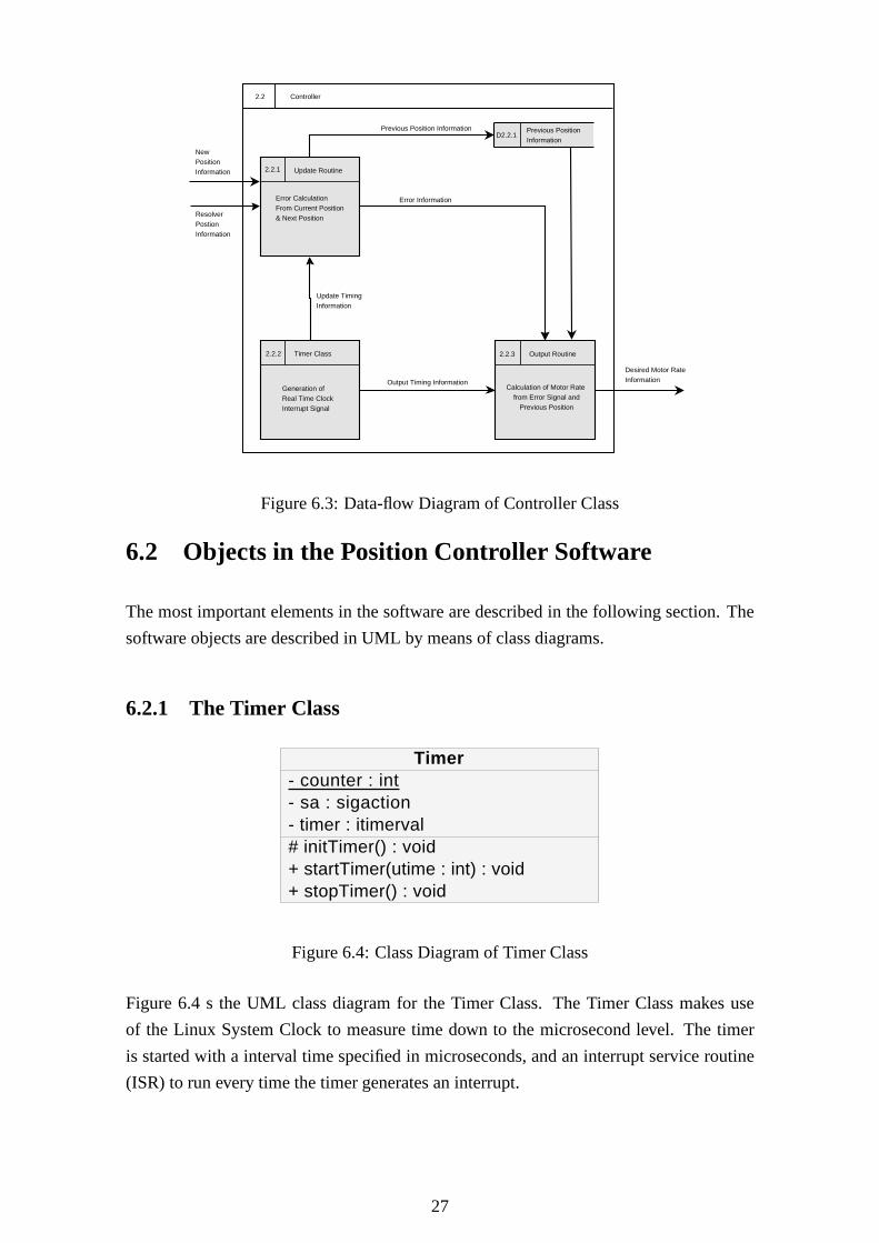
The data-flow diagram in figure 6.3, demonstrates how the controller class calculates
motor rate information from resolver position feedback andthe desired position input.
25

Calculating ControlSignals for the
Pedestal
2 Position Controller
3. PedestalInterface
1. Interface onClient Machine
Position Information & Requests
Motor Rate Information
Position Information
Figure 6.1: Data-flow Context Diagram of Position Controller
2 Position Controller
Motor Rate Information
Resolver PositionInformation
3. PedestalInterface
Handling of UserInterface
2.1 Main Program
Implementing theControl Loop
2.2 Controller
D2.1 Desired Behaviour
1.Client Machine
Current Position Information
Motor RateInformation
Desired BehaviourInformation
PositionInformation& Requests
Writing to DACReading from ADC
2.3 Pedestal Driver
D2.4 Current Position
Figure 6.2: Data-flow Level 1 Diagram of Position Controller
26
2.2 Controller
Error Calculation From Current Position�& Next Position
2.2.1 Update Routine
New PositionInformation
Resolver Postion Information
Generation ofReal Time Clock Interrupt Signal
2.2.2 Timer Class
Calculation of Motor Rate from Error Signal and
Previous Position
2.2.3 Output Routine
D2.2.1Previous PositionInformation
Previous Position Information
Error Information
Output Timing Information
Update TimingInformation
Desired Motor RateInformation
Figure 6.3: Data-flow Diagram of Controller Class
6.2 Objects in the Position Controller Software
The most important elements in the software are described inthe following section. The
software objects are described in UML by means of class diagrams.
6.2.1 The Timer Class
Timer- counter : int- sa : sigaction- timer : itimerval# initTimer() : void+ startTimer(utime : int) : void+ stopTimer() : void
Figure 6.4: Class Diagram of Timer Class
Figure 6.4 s the UML class diagram for the Timer Class. The Timer Class makes use
of the Linux System Clock to measure time down to the microsecond level. The timer
is started with a interval time specified in microseconds, and an interrupt service routine
(ISR) to run every time the timer generates an interrupt.
27

� � � � � � � � � � � �� � � � � � � � � � �� � � � � � � � � � � � �� � � � � � � � � � � � � � � � � � � � � � �
Figure 6.5: Class Diagram of Pedestal Driver Module
6.2.2 The Pedestal Kernel Module
The pedestal driver module as seen in figure 6.5 is a kernel module that runs in the kernel
memory space. It is a driver for a character device, and creates a file enter in the ’/dev/ ’
directory of the operating system called/navy/0. User-space applications can then open
this device as if it were a file, to read and write to it.
Reading from the Pedestal Kernel Module
When a ’read’ operation is called on the ’/dev/navy/0’ the driver module calls a function
which reads from the ADC, and stores the value in a string of characters. The ’read’
function handles all communication with the ADC circuit andneeds no input from the
user. The string returned by this function contains two signed integer values separated by
a comma. These two values correspond to the different windings on the position resolver.
The range of the output is from -2048 to 2047, which correspond to inputs to the ADC of
-10V to +10V.
Writing to the Pedestal Kernel Module
A ’write’ operation takes as a parameter an array of characters to be transmitted to the
DAC. This array is converted to an unsigned integer lying within the range of 0 to 4095.
0 will translate to an output voltage of 0 Volts on the DAC and 4095 will translate to an
output of 6V.
6.2.3 The Controller Class
In figure 6.6, the methods and attributes of the Controller Class are given. The public
methods that are used aregetPosition() to display the current position andsetPosition() to
set the new position. Theupdate() function is called whenever the Timer Class generates
a timeout interrupt and runs the designated ISR.
The controller class implements the control system for eachand calculates new values
every time theupdate() function is called. Therefore two instances of Class Controller
are initialised, one for the elevation plane, and one for theazimuth plane.
28

! " # $ % " & & ' %( ) * + , - . ) * / * 0 , 1 2( , 3 4 5 0 6 7 8 4 2( , 3 , 1 0 6 7 8 4 2( , 9 2 4 2 * 0 6 7 8 4 2( . : 4 , 1 0 6 7 8 4 2( . 8 - , 2 , 8 1 0 6 7 8 4 2; < 8 1 = * / 2 > 8 - ? @ A 6 6 * / 0 - 2 / , 1 B C 0 = 8 , DE B * 2 > 8 - , 2 , 8 1 ? C 0 6 7 8 4 2; - * 2 F 4 2 * ? / 4 2 * 0 , 1 2 C 0 = 8 , DE A . D 4 2 * ? C 0 = 8 , DE - * 2 > 8 - , 2 , 8 1 ? 1 * G H . 8 - , 2 , 8 1 0 6 7 8 4 2 C 0 = 8 , D
Figure 6.6: Class Diagrams of Controller Class
6.3 Sequence of Events in the Position Controller Soft-
ware
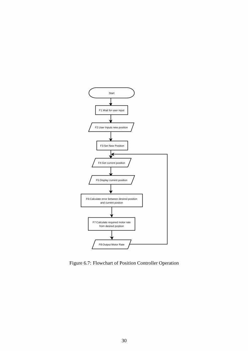
To describe the logical flow of the software a flowchart, figure6.7, is included. This
flowchart demonstrates the typical operation of the position controller. The flow begins
with a user input requesting a new position, and remains in a constant cycle until the
system is shutdown.
Since this system is a real-time system, figure 6.8 is a UML sequence diagram and in-
cludes estimated latency or run-times at each process step.
6.4 Software Testing
6.4.1 Pedestal Kernel Module
Read Function
Theread function was tested by attaching a variable power supply to the ADC and varying
the voltage supplied from -10 Volts to 10 Volts. The functionwas called at -10V, 0 V 10
V and a number of other random voltage levels. The ADC was thengrounded and 1000
conversion cycles were initiated and the results recorded.
Write Function
Thewrite function was tested by attaching the DAC to an oscilloscope and varying cycling
through the entire range of permissible DAC input codes. Theoutput voltage on the
oscilloscope was recorded and compared to the input code.
29
Start
F5:Display current position
F4:Get current position
F7:Calculate required motor ratefrom desired position
F8:Output Motor Rate
F6:Calculate error between desired positionand current postion
F2:User Inputs new position
F1.Wait for user input
F3:Set New Position
Figure 6.7: Flowchart of Position Controller Operation
30

F3: setPosition(pos : float)
F1: startTimer(utime : int)
F4: read() : string
F8: write(buffer : string)
I JKL MN K O OP N I QRS P N I TP UPV MW OX N RY P N I Z W N U[ W N P : User
I TKV R M R KL P N T N K\ N W S
F4: read ADC
F8: write to DAC
F5: showPosition()
F5: display position
: timer interrupt
F1: init()
F6: update()
F2: enterNewPostion(position)
Fig
ure
6.8
:U
ML
Seq
uen
ceD
iagram
for
Po
sition
Co
ntro
ller
31

Overall
The input of the ADC was connected to the output of the DAC, andthe DAC was cycled
through the entire range of possible input codes. The input was then compared to the
output.
6.4.2 Timer Class
An ISR was constructed that generated a pulse on one of the SBCports every time it
was called. The timer was set to the minimum interrupt time and was initialised to call
the ISR whenever a interrupt was generated. The port of the SBC was connected to an
oscilloscope and the output waveform was measured.
The timer was then set to generate an interrupt every 100 microseconds and the resulting
output waveform was recorded. The waveform was analysed andthe frequency and period
of the pulse on the waveforms was calculated, to be compared with the specified interrupt
time.
6.4.3 Controller Class
The controller class was tested by connecting the entire system except the motors together.
The position of the pedestal was held steady, while a new position request was input.
The voltage output of the motor drive circuit was expected toclimb to the minimum or
maximum level and was measured. The pedestal was moved past the new position and
the voltage was measured. The voltage was expected to move from either the minimum
or maximum level to the other extreme.
32

Chapter 7
Discussion of Results
This chapter describes the tests done and the results recorded in the actual implementation
of the position controller. The chapter deals with each partof the system seperately at first
and finally on to the position control system as a whole.
The results discussed in the chapter are for the azimuth axisonly, due to a non-functioning
elevation motor. However, the same circuit is used for the elevation axis and the motor
characteristic are identical, so the results are relevant for both axes.
7.1 Sampling Frequency of the ADC
The ADC driving software was programmed the ADC to convert continuously, in order
to measure the maximum achievable sampling rate with this configuration. The timing of
the ADC circuit’sbusy convert signal is shown in figure 7.1.
The sampling frequency,fs, was calculated to be 17.54kHz. , which is more much greater
than the required sampling frequency in equation 4.4.
7.2 Resolver Position Conversion
The resolver position circuit was tested in a number of different tests to aid in calculating
the overall accuracy, and the over all error in resolving theposition is calculated.
7.2.1 Power Supply to Analogue-to-Digital Converter Circuit
The power used to supply the ADC circuit was taken directly from the Cogent CSB337
through the general purpose input output (GPIO) expander, and there was a noise signal
33

0 50 100 150 200 250 300 350 400 450 500−2000
−1000
0
1000
2000
3000
4000
5000
6000
Time (µseconds)
Vol
tage
(m
V)
ADC Conversion Timing
Figure 7.1: ADCBUSY Signal
at 100 Hz with a peak-to-peak voltage of 420 mV. A low-pass filter with a -3 dB point
of 60Hz was introduced between the power supply and the ADCs.Not all the noise was
removed by the filter and the resultant power supply waveformis shown in figure 7.2
The noise is at a frequency of 100 Hz with a peak-to-peak voltage of 131mV, according
to the ADC specifications this will cause a degradation of input sensitivity by 3 LSB,
therefore the total error in the ADC defined in 4.2 increases to 3 LSB or 19.52 mV, so the
effective number of bits (ENOB) of the ADC is 9.
0 2 4 6 8 10 12 14 16 18 204300
4400
4500
4600
4700
4800
4900
5000
5100
Time (ms)
Vol
tage
(m
V)
Power Supply Noise
Figure 7.2: Power Supply Noise
7.2.2 Analogue to Digital Conversion Accuracy
The inputs to the ADCs were grounded and 1000 samples were taken, the results are
shown in figure 7.3. By examining figure 7.3, it is possible to calculate the effective error
34

of the ADCs, and these values are shown in table 7.1.
0 100 200 300 400 500 600 700 800 900 10000
2
4
6
8
10
Sample Number (fs = 17540Hz)
AD
C O
utpu
t
ADC X Output with Input at Ground
0 100 200 300 400 500 600 700 800 900 10000
2
4
6
8
10
Sample Number (fs = 17540Hz)
AD
C O
utpu
t
ADC Y Output with Input at Ground
Figure 7.3: ADC Output with Inputs at Ground
Table 7.1: ADC Conversion Error
ADC X ADC Y
Zero Offset 3 LSB (19.52mV) 3 LSB (19.52 mV)DC Error 2 LSB (9.76 mV) 4 LSB (39.04 mV)ENOB 9 bits 8 bits
The position is calculated by the arctan of the ratio of thesetwo voltages as in equation 3.4,
so the resultant error in the position is 4 LSB in 16 bits. Thismeans that the resolver
conversion has an resolution of 8 bits or 256 levels per 180o. Therefore the effective
accuracy of in measuring the position is±0.7oor 42 arc minutes.
The pedestal was moved with a constant angular rate, and the output of the conversion
was measured and is shown in figure 7.4. This shows that the accuracy was indeed within
42 arc minutes.
7.3 Digital to Analogue Conversion Accuracy
To measure the absolute accuracy of the digital to analogue converters, 3 different input
codes were tested and the output measured by an oscilloscope, the results are displayed
in figure 7.5.
The inputs codes, the expected outputs and the actual outputs are listed in table 7.2. Using
these results the maximum error of the DAC circuit is calculated to be:
35

0 500 1000 1500 2000 2500 3000 3500 40000
20
40
60
80
100
120
140
160
180
Time (ms)
Pos
ition
(D
egre
es)
Azimuth Position vs Time with Constant Angular Rate
Figure 7.4: Position Output for Constant Angular Rate
0 5 10 15 20 25 30 35 40 45 50
0
1000
2000
3000
4000
5000
6000
Time (µseconds)
DA
C O
utpu
t (m
V)
DAC Output for Zero, Half and Full Scale Input
Zero InputFull Scale InputHalf Scale Input
Figure 7.5: DAC Output for Different Input Codes
Table 7.2: DAC Performance
Input Code Expected Output Actual Output
0 0 V 0 V±0.5%2047 3 V 2.98 V±0.7%4097 6 V 5.91 V±0.7%
36

eDAC = 2.2%= 132 mV (7.1)
7.4 Overall Performance of Position Controller
The position controller was installed on the pedestal and the system was given a position
90 degrees from the current position. The rate output on the tachogenerator was recorded
by an oscilloscope, the output is shown in figure 7.6.
0 50 100 150 200 250 300 350 400 450 500−500
0
500
1000
1500
2000
2500
Time (msec)
Vol
tage
(m
V)
Tachogenerator Output vs Time
Figure 7.6: Motor Rate for Position Command
37

Chapter 8
Conclusions and Recommendations
This report demonstrates how a position resolver can be implemented onto a Navy pedestal
with an accuracy of 42 arc minutes succesfully, this chapterdraws conclusions from the
results in the previous chapter, and makes recommendationsbased on those concusions.
8.1 Position Resolver Accuracy
The accuracy was calculated as 42 arc minutes, and was shown to be within that specifica-
tion, but for any scientific purposes an antenna controller would need to be more accurate
than this.
8.1.1 Recommendations for Improving Accuracy
Regulated Power Supply
The power supply noise would be eliminated by a regulated power supply, and thus reduce
the noise on the resolver conversion process.
Printed Circuit Board Design
To eliminate the noise on the resolver conversion, the electronics should be moved to
a printed circuit board. The board on which it was designed causes interference and
crosstalk with the analogue to digital converter.
38

Resolver-to-digital Converter
A commercial resolver-to-digital converter could be purchased to replace the ADC cir-
cuitery and would offer far superior accuracy.
8.2 Position Controller Performance
Since the focus of this project was not on optimising the performance of the position
control loop, the performance of the position controller was examined in great detail. The
results of the position controller show that the performance is adequate and this position
control system can perform sufficiently well.
8.2.1 Recommendations for Improving Controller Performance
Since the writer of this report has little experience in control systems, an engineer with
some experience in this field would possibly be able to improve the performance of this
control system remarkably.
39

Appendix A
Resolver Module
40

Appendix B
Postioner Application
41

Bibliography
[1] Tips for using the ADS78xx Family of AD converters. Technical report, Texas
Instruments Incorporated, 2000.
[2] Cogent CSB337 Hardware Reference Manual, 2003.
[3] D. Abramovitch. Phase-Locked Loops: A Control Centric Tutorial. Technical re-
port, Agilent Labs,Palo Alto, May 2002.
[4] G. Arslan and F. A. Sakarya. Performance Evaluation and Real-Time Implementa-
tion of Subspace, Adaptive, and DFT Algorithms for Multi-tone Detection.Ptolemy
Project, 1996.
[5] K. Banks. The Goertzel Algorithm.Embedded Systems Programming, August 2002.
[6] R. Bliss. Navy Electricity and Electronics Training Series, 1992.
[7] M. Braae. Control Theory for Electronic Engineers. UCT Press, Cape Town, 7700
South Africa, 1994.
[8] A. R. . J. Corbet.Linux Device Drivers. O’Reilly Media, Sebastopol, CA 95472,
2001.
[9] J. Gasking. Resolver-to-digital Conversion - A Simple and Cost Effective Alterna-
tive to Optical Shaft Encoders. Technical report, AnalogueDevices, Massachusetts,
March 1992.
[10] J. Horn. ADS7809 TAG Feature. Technical report, Texas Instruments Incorporated,
2000.
[11] P. Horowitz and W. Hill.The art of electronics. Press Syndicate of the University of
Cambridge, Cambridge,CB2 1RP, 1989.
[12] M. F. Jimmy Mason. Efficient Algorithms and Implementation of a DTMF Detector.
Technical report, University of Texas at Austin, 1997.
[13] M. Y. Jin and C. Wu. Servos, Selsyns and Friends.Tech MusingsIEEE, 147:1–2,
May 2000.
42

[14] I. P. Johan Lilius. Modelling Embedded Software in UML.Technical report, Abo
Akedemi University, 2004.
[15] J. Kessler.Synchro Resolver Conversion Handbook, Fourth Edition. Data Device
Corporation, Bohemia, NY 11716, 1994.
[16] Y. Y. Z. Z. Lingxia Wang, Bo Yao. A Survey of Embedded Operating Systems,
2000.
[17] M. McClure. A Simplified Approach to dc Motor Modeling for Dynamic Stability
Analysis. Technical report, Power Supply Control Products, 2000.
[18] L. C. H. P. M. M.J. Humphreys, D. Brown.Power Semiconductor Applications.
Philips Semiconductors, Hazel Grove,SK7 4DF, 1994.
[19] N. Morrison. Introduction to Fourier Analysis. John Wiley and Sons, Inc, 1994.
[20] A. F. W. G. F. H. J. P. Randy Agosti, Dave Dayton.Synchro and Resolver Conver-
sion. Memory Devices Ltd, Surrey, KT8 0SN, 1987.
[21] S. W. Smith.The Scientist and Engineer’s Guide to Digital Signal Processing. Cal-
ifornia Technical Publishing, 1997.
[22] G. Thomas. Modelling the Azimuth Position Control System. Technical report,
University of Wales Swansea, 2001.
[23] T. Wescott. PID Without a PhD.Embedded Systems Programming, October 2000.
[24] J. S. P. W. Wookey, Chris Rutter.Guide to ARMLinux. Aleph One, Cambridge, CB5
9BA, 2001.
43