Eleventh FloorMenzies BuildingPO Box 11E, Monash UniversityWellington RoadCLAYTON Vic 3800 AUSTRALIA

Telephone: from overseas:(03) 9905 2398, (03) 9905 5112 61 3 9905 5112 or 61 3 9905 2398

Fax: (03) 9905 2426 61 3 9905 2426

e-mail impact@vaxc.cc.monash.edu.au

web site http://www.monash.edu.au/policy/

Paper presented at the 5th Conference on Global Economic AnalysisTaipei, June 2002

COBB-DOUGLAS UTILITY − EVENTUALLY!by

Alan A. POWELL

Keith R. MCLAREN

K. R. PEARSON

and

Maureen T. RIMMER

Monash University

Preliminary Working Paper No. IP-80 June 2002

ISSN 1 031 9034 ISBN 0 7326 1533 X

The Centre of Policy Studies (COPS) is a research centre at Monash University devoted to quantitative analysis of issues relevant to Australian economic policy.

CENTRE of

POLICYSTUDIES and

the IMPACTPROJECT

COBB-DOUGLAS UTILITY − EVENTUALLY !by

Alan A. POWELL Keith R. MCLAREN K. R. PEARSON Maureen T. RIMMER

Monash University

Abstract

Consider the following two opinions, both of which can be found in the literature of consumerdemand systems:

(a) As the real income of a consumer becomes indefinitely large, re-mixing the consumptionbundle becomes irrelevant: having chosen the ultimately satisfying budget shares at any givenset of relative prices, the superlatively wealthy continue to allocate additional income in thesame proportions. With very large and increasing per capita income, ultimately the utilityfunction becomes indistinguishable from Cobb-Douglas.

(b) Consumer demand systems in which the income elasticities monotonically approach one (fromabove, in the case of luxuries; from below, in the case of necessities) are unsatisfactory boththeoretically and empirically. For instance, a necessity with a low (< 1) income elasticity mayvery well become less elastic with further increases in income.

The issue is important for CGE modelers because explicit direct additivity (as in the linearexpenditure system [LES]) is often the modeler’s default choice: this leaves us firmly in the worldof (a). Hanoch’s implicit direct additivity exhibits very flexible Engel properties. Rimmer andPowell’s AIDADS system belongs to this class. Within such a system it is possible to satisfy themotivations underlying both (a) and (b), as illustrated by the Engel (income) elasticities for a 3-commodity AIDADS system shown below in Figure 1.Whilst the system eventually converges toCobb-Douglas, some income elasticities can be effectively zero at any imaginable actual incomelevel. Inferiority can also be accommodated over a range of incomes. This paper discusses theabove in more detail, strengthening the case for implicit direct additivity. An experimental cali-bration of a database to the AIDADS system is illustrated with modifications made to the ORANI-Gteaching model. A technical appendix establishes the effectively global regularity of AIDADS.

Key words: consumer demand system, applied general equilibrium, separability, implicitly directlyadditive preferences, effectively global regularity, Cobb-Douglas, calibration, AIDADS.

Introduction and historical reprise1

Given their typical dimensions, endowing AGE2 models with consumer demand parameters is anon-trivial task. Large one-country models such as MONASH (Dixon and Rimmer, forthcoming)involve more than 200 commodities (the local and the overseas-produced versions of 100+ genericcommodities). This means that the matrix of own and cross price elasticities has more than 2002

(i.e., >40,000) elements that must somehow be evaluated. In the case of the global GTAP model(Hertel ed. 1996) the number of potentially different demand parameters explodes even further. In

1 Without implicating them in any remaining errors, we wish to acknowledge the kindly assistance

provided by Ken Clements, W. Jill Harrison and Daina McDonald. The views expressed by Theil andClements in their monograph (1987) would identify them as adherents of proposition (b) in theabstract.

2 We use AGE (applied general equilibrium) and CGE (computable general equilibrium) throughout assynonyms.

2

such a world there is no possibility of telling (say) 20 graduate students each to go off andindividually estimate 200 parameters econometrically (which was the style of parameter evaluationused in early macrodynamic modelling).The methods used to ease the inferential load placed onavailable data have inevitably involved imposing structure on the underlying micro-behavioral (inthis case, utility) functions.

The Cobb-Douglas utility [CDU] function has been used in some early AGE work but it lies at theextreme end of a spectrum which has minimal required parameter knowledge at one end, and real-world realism at the other. Under CDU all own total expenditure elasticities are one, all own priceelasticities are minus one, and all cross price elasticities are zero, so no estimation at all need becarried out. Stone’s Linear Expenditure System (1954) made the minimal changes needed to breakthis parameter rigidity by displacing the CDU indifference map away from the origin. The LEScould be interpreted as a CD system in which the arguments of the direct utility function were notthe actual quantities consumed, but the extents to which these quantities exceeded the basic (orsubsistence) requirement of each. Conventional total expenditure elasticities of demand could nowbe less than, equal to, or greater than unity, and own and cross price elasticities escaped the CDstraightjacket.

Houthakker (1960) put on a rigorous basis an intuitive proposition that had been discerned as earlyas 1910 by Pigou (and further developed by Friedman (1935)): in its rigorous form it stated thatunder explicitly directly additive preferences (which apply in the case of the LES), cross-substitution elasticities σij are directly proportional to the product of the pair of total expenditureelasticities involved:(1) σi j i jE E= Φ ( )i j≠

This greatly reduced the cybernetic load that must be met by available data in order to estimatedemand behavior: instead of something of the order of n2 demand coeff icients (where n is thenumber of commodities), only n coefficients (n-1 expenditure elasticities Ei and one value of Φ )are needed to determine behaviour at any point in the n-dimensional commodity space.

The liabilities of the LES are usually listed as follows:

a. Equation (1) is too restrictive to accommodate substitution among commodities except at high levelsof aggregation; in particular, specific (as distinct from general) substitution effects are ruled out.

b. Complementary pairs of goods (σij ≤ 0) and inferior goods (Ei < 0) are ruled out.

c. All Marshallian own-price elasticities of demand ηii are less than one in absolute value unlesstheir corresponding subsistence parameter γi is allowed to be negative (destroying its sub-sistence interpretation).

d. Marginal budget shares [MBSs] are constant (whereas there is strong evidence that the MBS offood falls with increasing affluence).

An additional restriction imposed by the LES is:

e. Budget shares are monotonic in real expenditure (which is at variance with the empiricalevidence from household survey data − see Lewbel (1991) and Rimmer and Powell (1994)).

Relative to the above list, the advantages of implicit direct additivity as implemented in AIDADS are thatmarginal budget shares may vary with the level of real income per head, and, in common with Engelelasticities, are not necessarily monotonic in real expenditure. Further, under implicit direct additivityof preferences, inferior goods are allowed (Hanoch 1975, p.401). Finally, own price elasticities canexceed one in absolute value without requiring the corresponding γc to be negative.

3

The ORANI -G model

The 22-sector version of the ORANI-G model is a smaller and slightly simplified version of theORANI model (Dixon, Parmenter, Sutton and Vincent, 1982). ORANI-G is almost identical to theORANI-F model (Horridge, Parmenter and Pearson, 1993) when the latter is used in a policy-analytic closure; extensive documentation of ORANI-G can be downloaded from the Monash Centreof Policy Studies web site (http://www.monash.edu.au/policy/oranig.htm). ORANI-G has been usedin training courses as an introduction to AGE modelling and in preparation for more advancedinstruction for potential users of the MONASH model (Dixon and Rimmer, forthcoming).

Modifying the existing consumer demand system in ORANI -G

The consumer demand system in ORANI-G is specified as a two-level nest. At the lower level,domestically produced and imported goods of the same generic type are combined into a compositegood using a CES aggregator function. The utility-maximizing mix of composite goods is thenfound using the Stone-Geary utility function and the associated LES, which has the form:

(2) p x p mc c c c c ipii CON

= + −∈∑γ β γ ,

in which pc and xc respectively are the CES price and quantity indexes for the consumption ofcomposite good c, γc is the (constant) ‘subsistence’ minimum requirement of c, βc is the (constant)marginal budget share (MBS) of commodity c, m is total per capita consumption spending, andCON is the set of composite commodities that are consumed. Since the βc must add to unity, theparameters β and γ total (2n − 1) in number, where n is the number of goods in CON. Note that pcis the purchasers’ price of commodity c and m is reckoned at purchasers’ prices.

The invariant MBSs in LES are not plausible except as local approximations. As noted above, theMBSs and Engel elasticities for food have been shown to vary greatly with per capita income(Rimmer and Powell, 1993; Cranfield, Hertel, Eales and Preckel (1998); Coyle, Gehlhar, Hertel andWang (1998)).

The AIDADS3 specification achieves much greater Engel flexibility than LES at the expense of

additional parameters. It replaces (2) with

(3) p x p mc c c c c ipii CON

= + −∈∑γ φ γ

in which the φc are the following functions of the utility level u:

(4) φ α βc

c cu

ue

e= ++1 .

Since the αs, like the β s, must add to 1, AIDADS thus involves an additional n parameters —(n−1) independent values of α, and the origin u0 from which the utility level is measured. Thevariable φc behaves logistically, remaining always within the [αc , βc] interval.

The LES is nested within AIDADS: putting αc ≡ βc (for all c) results in identity between φ, α andβ. Thus it is the divergence of α from β that generates the enhanced Engel flexibility of AIDADS.An example of this flexibility in a 3-commodity world is illustrated in Figure 1. The limiting value

3 The acronym AIDADS stands for an implicitly directly additive demand system.

4

as income grows indefinitely large of c’s MBS is βc.irrespective of the comparative magnitudes ofαc and βc.

4

Figures 1 and 2 were constructed to illustrate the proposition eponymous with the title of this paper.The underlying parameter settings are thus close to the boundaries of the regular region of theparameter space in which all values of α, β and γ are non-negative, with the values of α and β eachadding to unity across commodities. The values of the parameters are shown in the panel below:

α1 α2 α3 β1 β2 β3 γ1 γ2 γ3 u0

0.826821810

43180600

0.059977419

77526710

0.113200769

79292700

0.000000000

01322384

0.999999999

98650700

0.000000000

000269011 5 0.2 0.18955332986

922400

Double precision is recommended for computations in cases like this (although with much manualintervention the curves in Figures 1 and 2 can be plotted using single-precision software). Exceptfor commodity 2, αc > βc and so the shares of commodities 1 and 2 approach very small numberswith increasing affluence. Figures 1 and 2 show that by the time the Engel elasticities of these twotemporarily inferior goods start to climb towards unity, their shares in the consumer’s budget havelong since become infinitesimal. Commodity 2’s budget share is very close to 100 per cent wellbefore the Engel elasticities of the other two commodities begin their dramatic eventual ascent.

The initial step in generalizing ORANI-G’s household demand structure was to rewrite the source(Tablo) code for the model and to ensure that the new model (ORANAIDAD ) could reproduceORANI-G results when α was set equal to β. The β and γ parameters were taken from the 1998Training Course version of ORANI-G, which used a 1987 Australian database. Using the latterdatabase, ORANI-G and ORANAIDAD were then presented with the same endowment shock a 5per cent increase in capital stocks and in agricultural land (where used as an input) in every sector in a closure in which real wage rates, aggregate real investment and real government spendingwere exogenous and in which employment was demand determined. The results obtained wereidentical to at least five decimal places for all macro variables.5 A selection of these results arepresented in Table 1.

Large Changes with LES and with AIDADS

A single LES that is, one with exactly one set of values for β and γ is not able to capturechanging consumption patterns across wide variations in living standards. Typically this problemhas been handled by making the γ values increasing functions of real income, or by appealing tochanges in taste (as in the MONASH model see Dixon and Rimmer (forthcoming)).One wouldexpect AIDADS to be able to handle large changes in per capita real incomes without the necessityof taste changes.

To put this into perspective, consider the 39-year period (from June 30th 2000 through July 1st

1960). Official estimates of real consumption per capita show a growth rate between 1960 and 2000of almost exactly 2 per cent per year. According to Lluch, Powell and Williams (1977), a key

4 These propositions may be checked from the formulae (18) and (19) below for ψc (the MBS of c).5 The original ORANI-G model was coded completely from its linearized equations, while ORANAIDAD was

coded as a mixture of levels equations and linearized equations. For a general discussion of the mixedapproach, see Harrison, Pearson, Powell and Small (1994).

5

coefficient in LES (the so-called Frisch ‘parameter’) responds strongly to per capita real income.6

As a result, if we stay within the LES specification, the values of the γ coefficients must, onaverage, have declined by about 24 per cent between 1960 and 20007.

The additional parameters available in AIDADS allow the γs to remain constant across the develop-ment spectrum (Rimmer and Powell, 1992). In the current context this means that we should beable to allow a divergence between the α and β parameter vectors to substitute for a change in γ asa means of having the demand system fit databases at two different points of time. Rimmer andPowell (1992) found that the Australian share of food in the consumer’s budget at widely separatedlevels of per capita income was consistent with invariant values of γ. Moreover, the values offood’s share at very low and at high per capita real incomes was consistent with cross sectionalevidence on differences in food’s budget share across nations at different stages of development(see Figure 3).

Calibration of A IDADS to the ORANI -G database8

The insertion of AIDADS into ORANI-G requires an exact mutual fit of the AIDADS demand systemand the base-case data. As the only available AIDADS estimates come at the six commodity level(Rimmer and Powell, 1992a and 1996), either a method must be found for allocating parametersfrom the 6-commodity system to the 23 commodities recognized by ORANI-G, or a less formalapproach must be substituted. We give examples of both. As the purpose of the current paper isillustrative, we must emphasize that these calibrations are exploratory: serious policy analysiswould require much more data work.

The LES parameters β, γ and ΦThe subsistence parameters γ in ORANI-G and in ORANAIDAD are notionally per capita variables. Itis convenient to normalize on the population applying to the base-case data. The units in which theγs are expressed, therefore, are real units of commodities per X people, where X is the base-casepopulation (about 18 million). Real units of commodities are the amounts that could be bought inthe base case at basic-value prices with one dollar. Population is exogenous in both models.

6 Consumption data were downloaded on line from the Australian Bureau of Statistics web site,

http://www.abs.gov.au/ausstats/abs%40.nsf/w2.3.1!OpenView&Start=1&Count=1500&Expand=6.2#6.2 ,Table 33. Household Final Consumption Expenditure, Chain Volume Measures; population data werealso downloaded from the ABS web site, Table 2. Population(a) by sex, States and Territories, 30June, 1901 onwards.

7 In Lluch, Powell and Williams (1977) [hereafter LPW, page 76], the negative of the supernumerary ratio

ω ≡ −

− ∑∈

mm pi

ii

CON γ (the so called Frisch ‘parameter’, to be interpreted within LES as the elasticity with

respect to total per capita nominal consumption spending of the marginal utility of the last dollar optimallyspent) for different countries is found empirically to follow the rule:

−ω = 0.36 mid-sample value of real gnp per head measured in 1970 US dollars– 0.36.

Thus −ω declines by about 0.36 percent for each one per cent increase in real income per head. Real per

capita income increased by about ([1.02]39 – 1) × 100 =116. 5 per cent over the 39-year period mentioned inthe text. Using the LPW relationship above, we find

–ω2000 = –ω1960 × (2.16 5 ) − 0.36 = 0.7574 × ( –ω1960 )8 This section draws freely on Rimmer and Powell (1992c).

6

The starting point for the calibration of ORANAIDAD is a review of the method used by Horridge(2001) for ORANI-G (which in turn is based on Dixon, Parmenter, Sutton and Vincent (1982)). Wehave seen from the Introduction that n-1 expenditure elasticities Ei and one value of Φ aresufficient to characterize consumer behavior in the LES. The ORANI-G database contains estimatesof these entities for the base-case data. In the case of Φ , the information is presented as the Frisch‘parameter’, ω ≡ [−Φ −1], which is the negative of the supernumerary ratio (see footnote 6). In thedatabase the value assigned to ω is −1.82. An alternative interpretation regardsΦ as an average, overall pairs of commodities, of the partial substitution elasticities between the members of each pair.9 Inthe ORANI-G database the average substitution elasticityΦ hence is put at about 0.55.

How are the values of the LES MBSs β and the subsistence parameters γ obtained from the Ecvalues and the Φ value in the database? Since the Engel elasticities Ec are the ratios of the MBSs βc

to the average budget shares Wc, we have immediately that

(5) βc c cWE=where Wc is the ratio in the database of consumer expenditure (at purchasers’ prices) on commodityc to total consumer expenditure (for all c ∈ CON).

The γ parameters are found as follows. First equation (2) is solved for γc:

(6) γ γβc c

c

cix m

ppi

i CON

= − −∈∑ ,

which may be reformulated as

(7) γγ

βc c

c

c c

ix

mx

m

mp

pii CON= −

−∈∑

1

(8) = −

xcc

cW1 Φ

β.

The xcs are the quantities of commodities c consumed (c ∈ CON); their respective units are theamounts of each composite commodity c that can be purchased at basic value prices of the basecase for $1. These values can be read directly from the database, as can the value of ω ≡ [−Φ −1].The final step consists of evaluating (8). Note that both γc and xc are per capita concepts so that twodatabases which were identical in all respects except for population would imply different values of γ.

The AIDADS parameters α, β, γ and u0

In the case of ORANAIDAD we start by specifying the γs. Initially we take these as the values justfound for the LES later we will change them parametrically. Solving (3) for the functions φc , weobtain for all c ∈ CON:

(9) φ γγ

γγc

c c c

i

c c c

i

p xm

p xm

mmp pi i

i CON i CON

= −−

= −−

∈ ∈∑ ∑

( ) ( )

(10) = − × − p xm

c c c( ) ( )γ ω

9 This interpretation (or something close to it) is implicit in Leser (1960) and in Lluch, Powell and Williams (1977,

p. 17), and explicit in Powell (1992). It avoids the strong cardinality of Frisch’s (1959) original approach.

7

To finish the job, we must settle on some values of the gaps between α and β for each commodity,and find at least one value of the origin u0 of the utility map that is consistent both with thedatabase and the chosen values of α, β and γ. In addition, the price and quantity data, together withthe parameter setting ( α, β, γ, u0), must constitute a regular point in the solution space of AIDADS.

To avoid the necessity of appealing in empirical work to trends or taste changes, the minimumneeds vector γ must be treated as a true parameter. It has been noted above that when large changesin living standards are involved, this is not possible in the LES. With Φ = 0.55 in the ORANI-Gdatabase, about 45 per cent of expenditure is needed to pay for subsistence in the base case. Thus ifreal income per head were to decline at 2 per cent per annum from its value in a base casecorresponding to the year 2000 to its value in historical 1960, then after the fall of about 46 per cent (=100 × [1.0239− 1]) in real income per head, about 98 per cent (= 100×0.45/0.46) of total expenditurewould, according to the LES, be needed in 1960 to purchase subsistence. So for the experimentalcalibration we shall introduce a new subsistence vector ϑ with elements ϑc (c ∈ CON), which is relatedto the γ vector obtained from the LES calibration above by

(11) ϑc = (1 − κ) γc

(for all c ∈ CON, where 0 ≤ κ ≤ 1). The scalar κ can be chosen to lessen the likelihood thatsubsistence requirements will exceed consumption. To illustrate we chose κ = 0.5 (subsistencerequirements ϑc of all commodities in the calibrated AIDADS are set at 50 per cent of the corres-ponding benchmark γ values from the LES calibration).

The gap between α and β − first approach

We have seen that it is the gap between α and β that is responsible for the flexible Engel propertiesof AIDADS. The next step is to allocate values of

(12) δ α βc c c≡ −( )

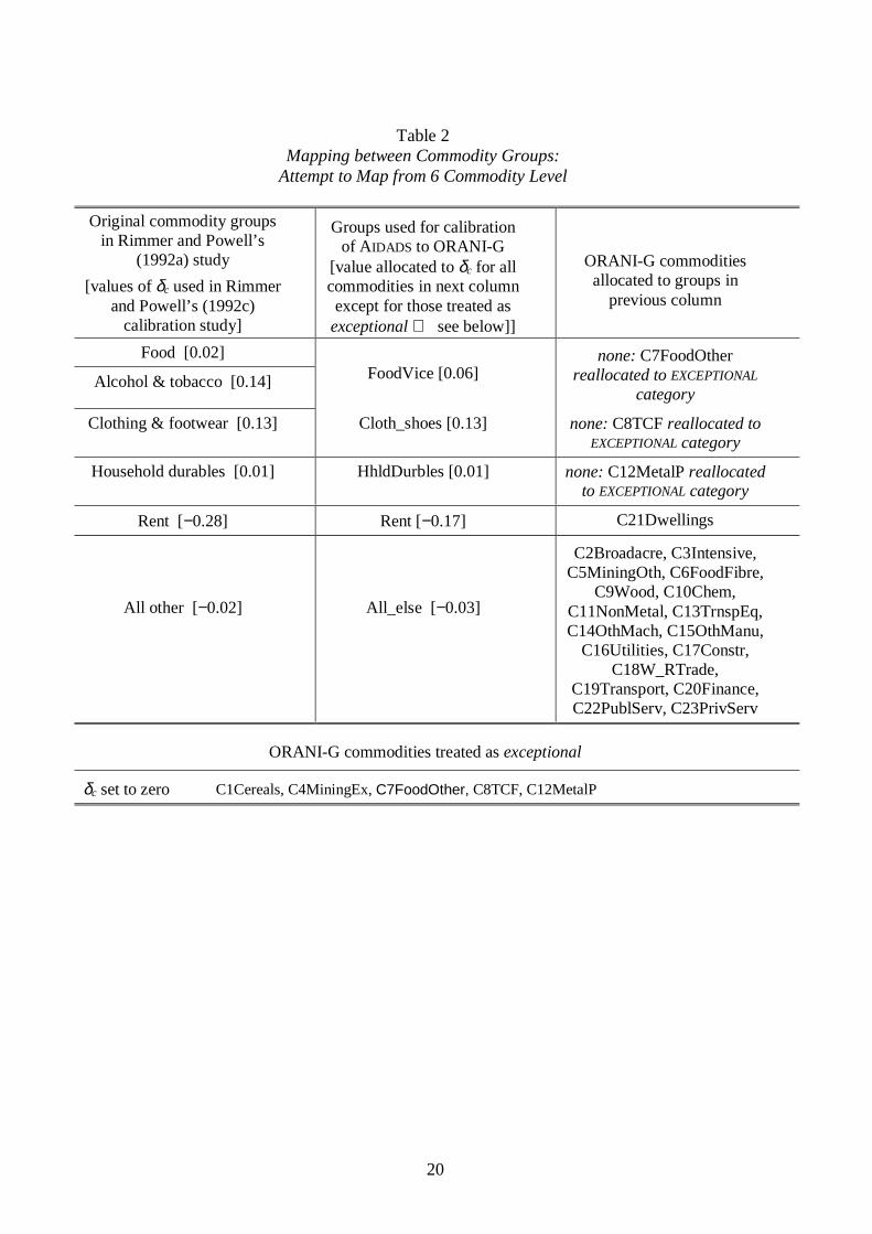
to the 22 ORANI-G commodities of which a non-zero amount is actually purchased by households(CON has 22 elements). Estimates of AIDADS at this level of disaggregation are not available; infact the only estimates for Australia of which we are aware are those made by Rimmer and Powell(1992a, 1996) at the six commodity level. A mismatch in the two aggregation schemes at thedetailed compositional level meant that only five groups for which estimates of δc were availablecould be distinguished in the present exercise. The details of the mapping used are shown in Table210.

Notice that, irrespective of the commodity grouping, the values of δc must sum over the membersof that grouping to zero. In Table 2 it can be checked that this applies in columns 1 and 2. After thevalues of δc in the second column were allocated to all the ORANI-G commodities of the thirdcolumn, this sum was no longer preserved. To correct this, the δc values transcribed from column 2to column 3 were renormalized so that they summed to zero:

(13) δ δ δc c ii CON

c gg REGULAR

W W* = −∈ ∈∑ ∑ /

10The allocation of some food raw materials to ‘All_else’ rather than to ‘Food’ reflects the fact that very

little of such primary commodities is sold directly to consumers (they buy the processed products inthe group ‘FoodOther’).

8

where the δ c* sum to zero by construction. The partition of the set of consumed commodities CON

into a REGULAR and an EXCEPTIONAL set arose because, given the settings for γ and u0 (where u0 isthe level of utility in the base case), it proved difficult to find a regular solution of the AIDADS

model in which the δ values of certain commodities differed from zero. These exceptional fivecommodities are listed in the lower part of Table 2.

How did these exceptions come about? The answer lies in the calibration of the values of α and β(as distinct from their differences). This is linked via equation (4) to the choice of the origin u0 ofthe preference map. Using (4) we find that

(14) α φ δc c

cu

u

e

e= +

+

0

01 and β φ δ

c cc

ue= −

+1 0

The only admissible values of u0 are those which yield values of αc and βc in (14) which are allpositive. In the current calibration exercise the approximate region of admissible values of u0 wasquickly established because the partial derivatives of αc and βc (with fixed values of φc and δc)differ in sign, it was found that a value of u0 which yielded non-negative β for all commodities hada tendency to yield some values of α which are negative (and vice-versa).

Using (9), from (14) it can be shown that preserving the non-negativity of the αs and βs requiresthat each γc must not exceed the smaller of:

(15)

( )

( )

( )

11

1 1

+ +−

+

!

"

$

###

+ +

≠∑

e xm p e

p e

e

u

u

c

rr c

r cu

cu

c

γ δ

δ

and

(16)

( )

( )1

1

1

+ −−

+

!

"

$

###

+ −

≠∑

e xm p

p e

e

u

u

c

rr c

r c

cu

c

γ δ

δIf γc exceeds (15) for any c, the corresponding αc is negative; if γc exceeds (16), then βc is negative.In calibrating AIDADS it is important to ensure that the above inequalities are respected.

When it appeared that the αs and βs for a pair of the commodities could not be calibrated for thegiven choice of δ s, equality of αc with βc was imposed for each such commodity. This led to afurther three commodities causing violation of the above condition; they were treated similarlywithout causing further violations.

Unfortunately, the net effect of the above procedure was to reduce the number of groups havinginitially differing gaps between the α and β values of their respective members to just two: theservices of the housing stock (Dwellings) and all other non-exceptional commodities. The base-caseEngel elasticity for Dwellings at 1.57 is the highest of the initial values in the ORANI-G database. Thisgives some point to the partition of δ values used here.

After the exceptional commodities had been identified, the value of u0 was set at a valuewhich yielded positive values of α and β for all REGULAR commodities. With the fixed set of γ valuesadopted, and the δs shown in Table 2, the value u0 must not exceed –3.41 (since otherwise the α

9

value for C5MiningOth becomes negative) − the value actually adopted was u0 = −4. The βc (andidentical αc) values for the exceptional commodities were left at the calibrated LES values for βc.

The final step in the calibration is to ensure that, demand parameters aside, the existing ORANI-Gdatabase is consistent with the fitted AIDADS system. This is accomplished by simulating a zeroshock to the newly calibrated model and checking that the original database is reproduced as thesolution.

Unfortunately the above method failed in any practical sense: the calibrated value of δ forcommodity C21Dwellings (the services of the housing stock) came out at –0.026, which had theexpected sign, but was far too small to be consistent with the 5+ percentage point rise in Dwelling’share of the consumer budget (from under 15 to more than nineteen percent since 1960).

The gap between α and β − second approach

The second approach to determining δ is more stylized. We note that the two ORANI-G commoditieswith the largest budget shares in the database are C7FoodOther (12.5%) and C21Dwellings (17.6%).These two commodities, accounting for more that 30 per cent of the consumer’s budget betweenthem, are also the two for which available evidence most forcefully suggests substantial slopes,negative and positive respectively, of their Engel curves.11

The value chosen for δc (c ←→ C21Dwellings) was –0.2 (which is less than the rather large valuefound econometrically for ‘Rent’, –0.29, by Rimmer and Powell (1992a)). For the twentycommodities other than C7FoodOther and C21Dwellings, δ values were set to zero (as in the LES).Because δs must sum to zero, the choice of the above value for dwellings implies that δc (c ←→ C7FoodOther) is +0.2. The adopted value of u0, at u0 = 0, was chosen to be just slightly higher thanthe lowest value (–0.0260) at which the non-negativity of all αs and βs could be guaranteed by theinequalities discussed above. The resulting allocation of δ-values is shown in Table 3.

Engel (total expenditure) elasticitiesWhilst the Engel elasticities Ec (= βc/Wc) in ORANI-G in the base case are supplied externally as partof the database, they are not invariant during simulations. Under AIDADS the Engel elasticities are:

(17) εi = ψi /Wi (i= 1, 2, ..., n)

in which the marginal budget shares ψi ≡ pi ∂xi/∂M are

(18) ψi = φi – (βi – αi)Ξ (i= 1, 2, …, n)

In (16) the coefficient Ξ is

(19) Ξ =

Σi=1

n

(βi − αi) ln (αi + βieu)− ln(pi) −

(1 + eu)2

eu

–1

.

It is shown in Appendix 1 that a necessary condition for the regularity of AIDADS at any point in theconsumer’s choice space is that Ξ is negative; and also that if starting from any regular point weincrease real income at fixed relative prices, then (in contrast to Deaton and Muellbauer’s (1980)AIDS), all such further points yield regular points. That is, AIDADS is effectively globally regular.

The reduction of all γc values to 50 per cent of their values as calibrated in LES drives the systemcloser to Cobb-Douglas at any given setting of the gaps between α and β. Setting all those gaps to

11 On the slope of the Engel curve for food, see e.g, Theil and Clements (1987); Rimmer and Powell (1992b); on theslope of the Engel curve for the services of the housing stock in Australia, see Rimmer and Powell (1992a ,b ;1996) .

10

zero results in a LES in which there is a dramatic narrowing of the spread of values of the base-caseEngel elasticities Ec, as shown in the panel below:

LES AIDADS

Original LES setting of γ[ORANI-G]

γ values set to 50% of ORANI-Gsetting [with all δ values zero]

γ values set to 50% of ORANI-Gsetting [δ values as in Table 3]

Min Ec 0.119 [C1Cereals] 1.000 [C1Cereals] 0.365 [C7FoodOther]Max Ec 1.573 [C21Dwellings] 1.701 [C5MiningOth]] 1.520 [C21Dwellings]

If the δs are set to the values shown in Table 3, the reduction in γ values still results in a narrowingof the spread in Engel elasticities, but to a lesser extent (compare the second and fourth columnsabove).

A Test Simulation with ORANAIDAD

With the δ-values set as in Table 3, a test simulation was conducted to check the behaviour of theORANAIDAD model. The effectively global regularity of AIDADS means that the system is less likelyto stray outside the model’s regular region when the living standard increases than in the case inwhich it falls (see Appendix 1). For the trial simulation it was decided to simulate a substantial fallin real per capita income.

The model was implemented using release 7 of the GEMPACK software suite12. Linearization errorswere controlled using the automatic accuracy facility of GEMPACK. The negativity of Ξ waschecked continuously throughout the computation.

The closure was not chosen on historical grounds, but rather to see how the model (and inparticular, its consumer-demand equations) would stand up to a large negative shock. The salientfeatures of the closure are shown in Table 4. The shock selected was a 25 per cent reduction in theproductivity of primary factors. Some macro results are shown in the panel below:

change [c] or % change [p]

real consumption per head p = −36.15

utility c = −0.7162

Ξ [must remain negative] [level] −0.2687→ −0.2366

real GDP p = −20.482

aggregate employment p = 0.402

nominal exchange rate p = 15.790

gdp deflator p = 10.528

real devaluation p = 4.752

import volume p = −17.554

export volume p = −18.782

While the 20+ per cent drop in real GDP is a large change13, even larger changes occur in somevariables at the disaggregated level. The industry with the greatest fall in output is private services

12 See Harrison and Pearson (1996); more information is available from the web at http://www.monash.edu.au/policy/gempack.htm

11

(I23PrivServ), where the fall exceeds 48 per cent. The Engel elasticity for the output of thisindustry at 1.1047 is the third largest among the 23 commodities. About 73 per cent of the output ofprivate services is sold to households in the base case. These considerations cause us to expect alarge fall in activity in I23PrivServ (but more work would be needed to firm up on the 48 per centfigure).

The somewhat surprising increase of 0.4 per cent in aggregate employment (reckoned using wagebill weights) is made up of a drop in unskilled employment of 1.77 per cent that is more than offsetby an increase in skilled employment of 2.27 per cent. It follows that industries that demandrelatively skilled labour must have fared better in the simulation than industries in which theemployment mix is intensive in unskilled labour. Unravelling the employment result would have tostart with the extremely uneven compositional profile of the changes in capital rentals: thoughmostly negative, the changes experienced in the rental prices of capital in the 23 industries rangefrom +62 per cent (I16Construction) to –97 per cent (I21Dwellings). These are very large changesin relative prices they rule out the use of macro analogue equations for rationalization of theresult.

Concluding Remarks

Implicitly directly additive preferences provides much greater flexibility of Engel responses thanthe linear expenditure system, accommodating non-monotonic responses of Engel elasticities toincreasing affluence. The example used in this paper, the AIDADS demand system, has been shownto remain regular under a very large reduction in income in ORANAIDAD , an extension of theORANI-G model. A rigorous statement concerning the effectively globally regular status of thesystem has been addressed in the Appendix.

13 Keep in mind that, because of the homogeneity of CGE models, the absolute size of percentage changes

does not constitute the criterion for ‘large’ changes: rather it is the size of changes in ratios of realvariables or of prices. Yet the requirement that consumption of every good c exceeds its correspondingsubsistence parameter γc in the LES and in AIDADS does mean that the absolute size of contractions inoutput per head of population is relevant.

12

REFERENCES

COOPER, Russel J., Keith R. McLaren and Gary K. K. Wong (2002) ‘Modelling Regular andEstimable Inverse Demand Systems: A Distance Function Approach’, unpublished workingMS available from Dr Gary Wong, School of Economics, Faculty of Business and Law,Deakin University, Waurn Pond, Vic 3217 Australia.

COOPER, R.J., K.R. McLaren and Priya Parameswaran (1994) "A System of Demand EquationsSatisfying Effectively Global Curvature Conditions", Economic Record Vol. 70, No. 208, pp.26-35 (March).

COOPER, Russel J. and Keith R. McLaren (1992) ‘An Empirically Oriented Demand System withImproved Regularity Properties, Canadian Journal of Economics, Vol. 25, pp. 652-67.

COYLE, W., M. Gehlhar, T. Hertel and Z. Wang (1998): ‘Understanding the Determinants ofStructural Change in World Food Markets’, American Journal of Agricultural Economics,Vol. 80, No. 5, pp.1051-1061.

CRANFIELD, J., M., T. Hertel J. Eales and P. Preckel (1998): ‘Changes in the Structure of GlobalFood Demand’, American Journal of Agricultural Economics, Vol. 80, No. 5, pp.1042-50.

CRANFIELD, John A. L., Paul V. Preckel, James S. Eales and Thomas W. Hertel (1998): ‘On theEstimation of “An Implicitly Additive Demand System’, unpublished MS, PurdueUniversity, Department of Agricultural Economics, 1998.

DEATON, Angus and John Muellbauer (1980) ‘An Almost Ideal Demand System’, AmericanEconomic Review, Vol. 70, pp. 312-26.

DIXON, Peter .B., B.R. Parmenter, John Sutton and D.P. Vincent, (1982) ORANI: A MultisectoralModel of the Australian Economy (Amsterdam: North Holland Publishing Company)..

DIXON, Peter B. and Maureen T. Rimmer (forthcoming) Dynamic, General Equilibrium Modellingfor Forecasting and Policy: a Practical Guide and Documentation of MONASH (Amsterdam:North Holland ).

FRIEDMAN, Milton (1935) ‘Professor Pigou’s Method for Measuring Elasticities from BudgetaryData’, Quarterly Journal of Economics, Vol. 50, pp. 151-63.

FRISCH, Ragnar (1959) ‘A Complete Scheme for Computing All Direct and Cross DemandElasticities in a Model with Many Sectors’, Econometrica, Vol. 27, pp. 177-96.

GEHLHAR, Mark, and William Coyl ‘Global Food Consumption and Impacts on Trade Patterns’, inChanging Structure of Global Food Consumption and Trade (Washington, D.C., UnitedStates Department of Agriculture, Economic Research Service) WRS-01-1, pp. 4-13.

HANOCH, Giora (1975) ‘Production and Demand Models with Direct or Indirect ImplicitAdditivity’, Econometrica, Vol. 43, No.3 (May), pp. 395-420.

HARRISON, W. Jill and K.R. Pearson (1996) ‘Computing Solutions for Large General EquilibriumModels using GEMPACK’, Computational Economics, Vol. 9, pp. 83-127.

HARRISON, W. Jill, K.R. Pearson, Alan A. Powell and E. John Small (1994) "Solving AppliedGeneral Equilibrium Models as a Mixture of Linearized and Levels Equations",Computational Economics, Vol. 7, pp. 203-23.

HERTEL, T. W., ed., (1996) Global Trade Analysis: Modeling and Applications, (New York andCambridge: Cambridge University Press).

13

HORRIDGE, J.M., B.R. Parmenter and K.R. Pearson (1993) ‘ORANI-F: A General EquilibriumModel of the Australian Economy’, Economic and Financial Computing, Vol. 3, No. 2(Summer), pp. 71-140.

HORRIDGE, J.M., B.R. Parmenter and K.R. Pearson (1998) ‘ORANI-G: A General EquilibriumModel of the Australian Economy’. Edition prepared for Course in Practical GE modelling,Centre of Policy Studies and Impact Project, Monash University, June 29th – July 3rd 1998.May be downloaded from http://www.monash.edu.au/policy/oranig.htm.

LEWBEL, A. (1991) ‘The Rank of Demand Systems: Theory and Nonparametric Estimation’,Econometrica, Vol. 59, No. 3 (May), pp. 711-30.

LESER, C.E.V. (1960) ‘Demand Functions for Nine Commodity Groups in Australia’, AustralianJournal of Statistics Vol. 2, No. 3 (November), pp. 102-13.

LLUCH, Constantino, Alan A. Powell and Ross A. Williams (1977) Patterns in Household Demandand Savings (New York: Oxford University Press for the World Bank), pp. xxxii + 280.

PIGOU, A.C (1910) ‘A Method of Determining the Numerical Values of Elasticities of Demand’,Economic Journal, Vol. 20, No. 2, pp. 636-40..

POWELL, Alan A. (1992) ‘Sato's Insight on the Relationship between the Frisch 'Parameter' and theAverage Elasticity of Substitution’, Economics Letters, Vol. 40, No. 2 (October), pp. 173-5.

RIMMER, Maureen T., and Alan A. Powell (1992a) ‘An Implicitly Directly Additive DemandSystem: Estimates for Australia’, Impact Project Preliminary Working Paper No.OP-73(October).

RIMMER, Maureen T., and Alan A. Powell (1992b) ‘Demand Patterns across the DevelopmentSpectrum: Estimates of AIDADS’, Impact Project Preliminary Working Paper No.OP-75(December).

RIMMER, Maureen T., and Alan A. Powell (1992c) ‘The Implementation of AIDADS in theMONASH Model’, Impact Project unpublished Research Memorandum (10 December).

RIMMER, Maureen T., and Alan A. Powell (1994) ‘Engel Flexibility in Household BudgetStudies: Non-parametric Evidence versus Standard Functional Forms’, Impact ProjectPreliminary Working Paper No.OP-79 (June).

RIMMER, Maureen T., and Alan A. Powell (1996) ‘An Implicitly Additive Demand System’,Applied Economics, Vol. 28, No.12 (December), pp. 1613-22.

STONE, Richard (1954) ‘Linear Expenditure Systems and Demand Analysis; An Application to thePattern of British Demand’, Economic Journal, Vol. 64, No. 255 (September), pp. 511-27.

THEIL, Henri and K.W. Clements (1987) Applied Demand Analysis− Results from System-wideApproaches (Cambridge, Massachusetts: Ballinger).

14

Appendix 1

THE EFFECTIVELY GLOBAL REGULARITY OF AIDADSby

Keith R. McLAREN, Alan A. POWELL and Maureen T. RIMMER

Monash University

1. Purpose of this appendix

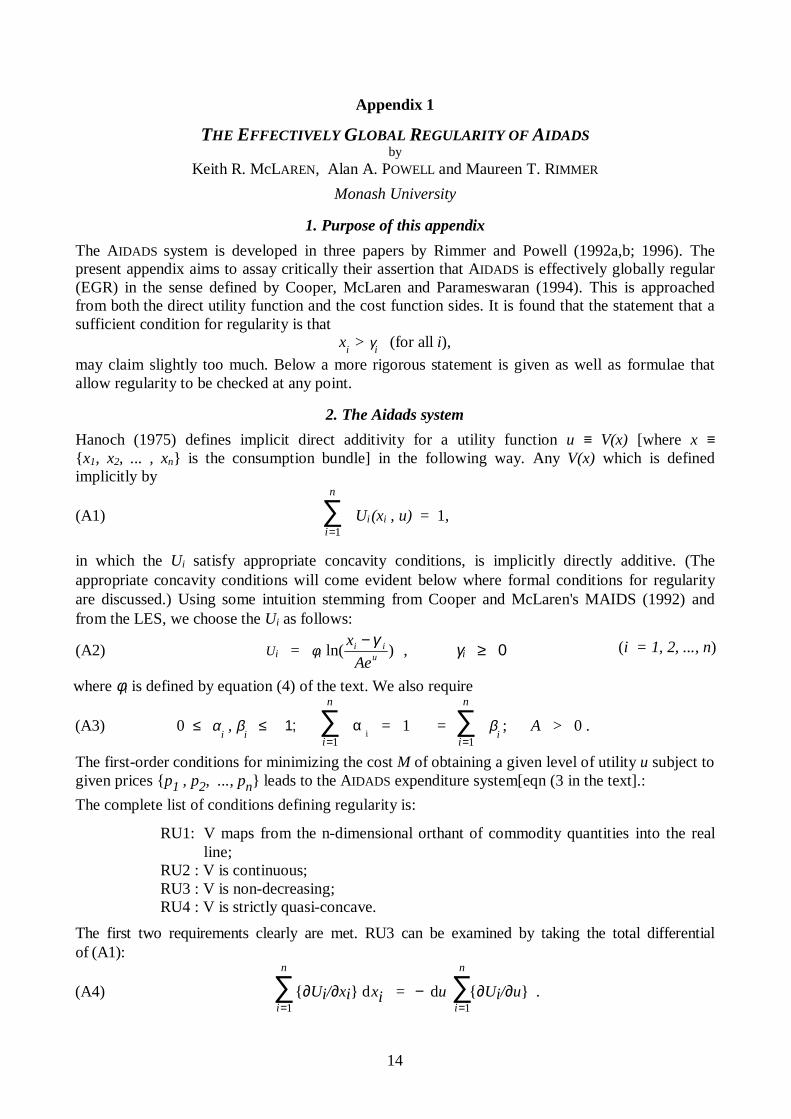
The AIDADS system is developed in three papers by Rimmer and Powell (1992a,b; 1996). Thepresent appendix aims to assay critically their assertion that AIDADS is effectively globally regular(EGR) in the sense defined by Cooper, McLaren and Parameswaran (1994). This is approachedfrom both the direct utility function and the cost function sides. It is found that the statement that asufficient condition for regularity is that

xi > γ

i (for all i),

may claim slightly too much. Below a more rigorous statement is given as well as formulae thatallow regularity to be checked at any point.

2. The Aidads system

Hanoch (1975) defines implicit direct additivity for a utility function u ≡ V(x) [where x ≡ x1, x2, ... , xn is the consumption bundle] in the following way. Any V(x) which is definedimplicitly by

(A1)i

n

=∑

1Ui (xi , u) = 1,

in which the Ui satisfy appropriate concavity conditions, is implicitly directly additive. (Theappropriate concavity conditions will come evident below where formal conditions for regularityare discussed.) Using some intuition stemming from Cooper and McLaren's MAIDS (1992) andfrom the LES, we choose the Ui as follows:

(A2) Ui = φi ln( )x

Aei i

u

− γ , γi ≥ 0 (i = 1, 2, ..., n)

where φi is defined by equation (4) of the text. We also require

(A3) 0 ≤ αi , β

i ≤ 1;

i

n

=∑

1α

i = 1 =

i

n

=∑

1β

i ; A > 0 .

The first-order conditions for minimizing the cost M of obtaining a given level of utility u subject togiven prices p1 , p2, ..., pn leads to the AIDADS expenditure system[eqn (3 in the text].:

The complete list of conditions defining regularity is:

RU1: V maps from the n-dimensional orthant of commodity quantities into the realline;

RU2 : V is continuous;RU3 : V is non-decreasing;RU4 : V is strictly quasi-concave.

The first two requirements clearly are met. RU3 can be examined by taking the total differentialof (A1):

(A4) i

n

=∑

1 ∂Ui/∂xi d xi = − du

i

n

=∑

1 ∂Ui/∂u .

15

Since all the partial derivatives ∂Ui/∂xi are positive, the issue hangs on the sign of Σi ∂Ui/∂u. Anexpression for the latter can be developed from (A2):

(A5)i

n

=∑

1 ∂Ui/∂u =

eu

(1 + eu)2

Σi=1

n

(βi − αi) ln (xi – γi) − (1 + eu)2

eu

(A6) = Ξ −1 eu

(1 + eu)2

where14

(A7) Ξ =

Σi=1

n

(βi − αi) ln (xi – γi) − (1 + eu)2

eu

–1

.

Since (1 + eu)2

eu is strictly positive, RU3 will be satisfied provided Ξ is negative; that is, provided Ξ−1

is negative. It is not obvious that Ξ is uniformly negative in regions in which every xi exceeds itsrespective γi. This is about as far as our discussion of RU3 will take us. We note that the negativity

of Ξ must be checked since Ξ < 0 is a necessary condition for regularity.

What of RU4? Paralleling the LES closely, the substitution elasticities in AIDADS are:15

(A8) σ i j = (xi – γi) (xi – γi)

xi xi / (M – p' γ)

M . (i≠j, i, j = 1, 2, ..., n)

in which p’γ is an abbreviation for the sum over i of piγi. From equation (4) of the text and the non-negativity of the αs and βs, the φs are also necessarily non-negative. Then from text equation (3) , ifM > p’γ, it follows that xi > γi for all i, and all (cross) substitution elasticities are positive; this issufficient to ensure that the implicit function V is strictly quasi-concave.

3. Insights from the differential of the indirect utility function

The differential of utility as a function of the differentials in prices and total expenditure may bewritten16

(A9) du = − (1 + eu)2

eu Ξ i

n

=∑

1φi d ln Ai ,

in which the Aj are:

(A10) Aj = (M – p′ γ) /pj

An increase in Ai represents a loosening of the budget constraint in the sense that the point wherethe budget hyperplane cuts the xi axis moves away from the origin when Ai becomes larger. Nowallow any one price (say pj) to decline slightly with M and the other prices fixed. From (A10), all Aj

must have increased, so the budget hyperplane must unambiguously have moved outward. Rationalbehaviour then implies du in (A9) is positive. This implies that in any regular region, the RHS of

14 A dual expression for Ξ in terms of prices and total expenditure is given above in the text as eqn (19).15 This is just an application of formulae provided in Hanoch (1975).16 See Rimmer and Powell (1992a), p. 20.

16

(A9) is positive. Since each φi, being a logistic function, is bounded in [0,1], local regularity thus

requires that

(A11) Ξ < 0 .

(Note, that we have not ruled out inferior goods we can envisage circumstances in which somegoods are locally inferior without disturbing the regularity properties of AIDADS. This is taken upin the next section.)

To summarize, we have established the following necessary condition for local regularity:

In any regular region, Ξ must be negative.

This is precisely the necessary condition found from the primal approach above.

4. Insights from the AIDADS cost function

The AIDADS indirect utility function can be found, albeit in implicit form, as follows:

(i) Solve text eqn (3) for xi.

(ii) Substitute this expression for xi into (A1), obtaining

(A12) Ui = φi ln φi + ln (M – p′ γ) − ln pi − ln A − u .

(iii) Now substitute from (A12) into (A1) and simplify, obtaining the (implicit form of) theAIDADS indirect utility function (the form is implicit because the φi are functions of u):

(A13) u = −1 + i

n

=∑

1φi ln φi + ln

(M – p'γ)

A −

i

n

=∑

1φi ln pi .

The cost function C(u, p) is obtained by solving (A13) for M, obtaining:

(A14) M = C(u, p) = p’γ + Ae[1+u] × Πi

i

i

np

i

=

%&'

()*1

φ

φ

;

for discussion it is sometimes more convenient to write this as

(A15) M = C(u, p) = p′ γ + Ae[1+u] Πi

n

ii

=

−

1 φ φ

× Πi

n

pii

=1 φ

.

Conditions (RC) which guarantee the regularity of the demand system generating C are:

RC1 : C R n: × →Ω Ω1 (where Ω j is the non-negativeRC2 : C is continuous orthant of dimension j)RC3 : C is homogeneous of degree one in pRC4 : C is non-decreasing in pRC5 : C is non-decreasing in uRC6 : C is concave in p.

Duality establishes that these conditions are equivalent to RU. To verify that these RC are satisfied,rewrite (A15) as

(A16) M = C(u,p) = P1(p) + φ(u) × P2(p, u) ,

17

where P1 is the Stone-Geary index p′γ, P2 is the (variable-elasticities) Cobb-Douglas-like indexshown as the last multiplicand on the right of (4.4), and φ(u) is the middle term enclosed withincurly parentheses on the right of (A15).

RC3 is the first condition needing discussion. At any given value of u, P1 and P2 are linearlyhomogeneous, and φ(u) is strictly positive; hence the condition is satisfied. Given the sign constraints(A3), a sufficient condition for RC4 to be satisfied is the side condition on (A2); namely,

(A17) γi ≥ 0 (all i).

Because RC6 is simpler than R5, we discuss RC6 first. In (4.6), P1 and P2 are each concave in p,and φ(u) is strictly positive. Hence their positive linear combination, C(u, p) also is concave andRC6 is established.

Preliminary to an attempt to establish RC5, we abbreviate Ae[1+u] × Πi

i

i

np

i

=

%&'

()*1

φ

φ

as T. Then

from (A14),

(A18) sign of ∂C/∂u = sign of ∂T/∂u = sign of ∂ ln T ∂u

.

To find out the sign of ∂ ln T/∂u, we proceed to take the derivative as follows:

(A19)∂ ln T ∂u

= 1 + i

n

=∑

1

∂ φi

∂u [ln (pi ) − ln (φi)]

From text eqn (4) we find

(A20) ∂φi

∂u =

eu

(1 + eu)2 (βi − αi) ;

while from text eqn (3), we see that

(A21) ln (pi) − ln (φi) = ln (M – p′ γ) − ln (xi – γi)Substituting from (A20) and (A21) into (A19), we find:

∂ ln T ∂u

= 1 + eu

(1 + eu)2 Σ

i=1

n

(βi − αi) ln (M – p′ γ) − ln (xi – γi)

(A22) = − eu

(1 + eu) 2 Ξ –1

The term eu

(1 + eu)2 is strictly positive, being a function of u with domain (-∞, +∞) and range

(0, 0.25]. Hence it follows that:

C(u, p) is increasing in u in any region in which Ξ is negative;i.e., negativity of Ξ is sufficient to guarantee the positive monotonicity of C in u.

This is just the condition required for u = V(x) to be increasing in x and (as found above) is anecessary condition for local regularity using the direct-utility-function approach.

18

Inferior goods? We now turn to the question: Can local inferiority of goods exist in AIDADS

without violating RC5? Given that Ξ is negative and that φi is bounded in [0, 1] for all i, from texteqn (16) we see that the ith marginal budget share will be negative in a regular region if and only if

(A23) (αi – βi )−Ξ > φi .

Inequality (A23) cannot be satisfied unless αi > βi. With αi > βi, φi → βi as u → ∞, while thepositive magnitude -Ξ → 0; thus it is quite possible that (A23) holds. A case in point is thenumerical example discussed above in the text and illustrated in Figures 1 and 2.

Effective Global Regularity? Returning now to the specification in terms of the cost function,substitution of (A20) into (A19) gives the remaining condition for regularity as

β α β α φi i i i i ipe

e

u

u− ≥ −+

+ −∑ ∑1 62 7

1 6ln ln . 1

2

Since β αi i− =∑ 1 6 0, only relative prices matter. If βi = α i ∀i, this condition is satisfied for all

relative prices. As the β i deviate from the αi it will be possible to find extreme relative prices forwhich the condition is not satisfied. However, for any given set of relative prices, as u increases, thefirst term on the right-hand side diverges exponentially to − ∞, and the second term converges to aconstant as the φ i converge to βi, ensuring that there exists a value of u, and hence of real income,at which this regularity condition is satisfied. Therefore the AIDADS system is effectively globallyregular. This ensures that if the system is regular at the set of sample points, it will also be regularat future points coinciding with higher levels of real income, provided the relative price changes arenot too extreme in particular directions.

19

TABLES

Table 1

Simulation used to check that the LES had been successfullygeneralized to AIDADS in the ORANAIDAD model

Variable Value *

nominal exchange rate (%) 1.89341consumer price index (%) [exog; numeraire] 0endowment of all capital stocks (%) [exog] shock 5.00000endowment of all agricultural land (%) [exog] shock 5.00000aggregate employment (%) 2.74578real aggregate consumptiom (%) 3.16721aggregate real investment expenditure (%) [exogenous] 0real government spending (%) [exogenous] 0real GDP (%) 3.42405

real devaluation (%) 2.14708export price index (%) 0.78068export volume index (%) 12.72294import price index, cif $A (%) [exogenous] 1.89341import volume index, cif weights (%) 1.53982change in ratio of trade balance to GDP (proportion) 0.01351

* Identical results obtained from both the original ORANI-G model and from its ORANAIDAD extension when the parameter vectors α and β are identical in the latter model and set to the β vector from ORANI-G . All results except the last are percentage deviations from base case. The change in the trade balance is expressed as the change in its ratio to GDP.

20

Table 2Mapping between Commodity Groups:

Attempt to Map from 6 Commodity Level

Original commodity groupsin Rimmer and Powell’s

(1992a) study

[values of δc used in Rimmerand Powell’s (1992c)

calibration study]

Groups used for calibrationof AIDADS to ORANI-G

[value allocated to δc for allcommodities in next columnexcept for those treated asexceptional see below]]

ORANI-G commoditiesallocated to groups in

previous column

Food [0.02]

Alcohol & tobacco [0.14] FoodVice [0.06]none: C7FoodOther

reallocated to EXCEPTIONAL

category

Clothing & footwear [0.13] Cloth_shoes [0.13] none: C8TCF reallocated toEXCEPTIONAL category

Household durables [0.01] HhldDurbles [0.01] none: C12MetalP reallocatedto EXCEPTIONAL category

Rent [−0.28] Rent [−0.17] C21Dwellings

All other [−0.02] All_else [−0.03]

C2Broadacre, C3Intensive,C5MiningOth, C6FoodFibre,

C9Wood, C10Chem,C11NonMetal, C13TrnspEq,C14OthMach, C15OthManu,

C16Utilities, C17Constr,C18W_RTrade,

C19Transport, C20Finance,C22PublServ, C23PrivServ

ORANI-G commodities treated as exceptional

δc set to zero C1Cereals, C4MiningEx, C7FoodOther, C8TCF, C12MetalP

21

Table 3Mapping between Commodity Groups using a Simpler Scheme

Groups used for calibration of AIDADS to ORANI-G[value allocated to δc for all commodities in next

column]

ORANI-G commodities allocated to groups inprevious column

FoodVice [+0.20] C7FoodOther

Rent [−0.20] C21Dwellings

All_else [0]C1Cereals, C2Broadacre, C3Intensive,

C4MiningEx, C5MiningOth, C6FoodFibre, C8TCF,C9Wood, C10Chem, C11NonMetal, C12MetalP,

C13TrnspEq, C14OthMach, C15OthManu,C16Utilities, C18W_Rtrade, C19Transport,

C20Finance, C22PublServ, C23PrivServ

Table 4Closure of ORANAIDAD used in Trial Simulation:

the Main Exogenous Variables

Exogenous variables(name in Tablo source code)

Description [dimensions]

p3totp0cif

qx1capx1lnd

p_aprima1, a2, a3, a1mar, a2mar, a3mar, a4mar

a5mar, a1cap, a1lab_o, a1lnd, a1oct,a1_s, a2_s, a3_s, a1tot, a2tot

f5f1oct

f1lab_io

f1lab_o, f1lab_i, f1lab

delBx2tot_ix5totfx6

f4p, f4q f4p_ntrad , f4q_ntrad

f0tax_s, f1tax_csi, f2tax_csi, f3tax_csf5tax_cs, t0imp, f4tax_trad, f4tax_ntrad

consumer price index (numeraire) [1]foreign prices of imports [23]

populationall sectoral capital stocks [23]

all sectoral agricultural land [23]economy-wide primary factor saving

technical progress [1]all other technolgical change [various;

largest are 23×2×23]shift in pattern of government demands [23×2]

real unit cost of 'other cost tickets' [23]economy-wide wage shift ( = worker's real

wage in this closure) [1]wage shifters for occupations, industries & for both

[2, 23, 23×2 respectively]ratio of trade balance to GDP [1]

aggregate real investment1 [1]total real government spending [1]shifter on rule for stocks [23×2]

shifters for traditional exports demand curve [both 1]shifters for non-traditional export demand [both 1]

all tax rates [1] − tax rates are uniform across theirrespective tax bases]

1 The investment allocation equation in the Tablo source code of ORANI-G was modified so that there was nochange in the sectoral allocation of the exogenous total. Since the latter is not shocked, all sectoral investment iseffectively set exogenously to zero change.

22

FIGURES

-0.4

-0.2

0

0.2

0.4

0.6

0.8

1

1.2

1.4

1.6

3 8 13 18 23 28 33 38 43 48 53

natural logarithm of real per capita total expenditure

Engel elas1

Engel elas2

Engel elas3

Figure 1: Behaviour of Engel elasticities in an AIDADS demand system in which allthree commodities initially are superior goods (their Engel elasticities arepositive), and in which two pass through an inferior phase.

-0.4

-0.2

0

0.2

0.4

0.6

0.8

1

0 5 10 15 20 25 30 35 40 45 50

share 3

share 2

share 1

natural logarithm of per capita real expenditure

Figure 2: Behaviour of commodity shares in the AIDADS demand system whose Engelelasticities are shown in Figure 1.

23

0

0.1

0.2

0.3

0.4

0.5

0.6

0 1000 2000 3000 4000 5000

Food

total per capita consumption expenditure (international dollars)

international cross sectionAustralian time series 1954-1989

backward extrapolation of Australian time-series data

Figure 3: Behaviour of food’s budget share under AIDADS estimated from 1975cross sectional international comparisons data and from Australiannational accounts time series data. The lowest income country in the datais India and the highest the USA. (Source: Rimmer and Powell (1992).