Eliciting Private Information with Noise: The Case ofRandomized Response∗

Andreas Blume† Ernest K. Lai‡ Wooyoung Lim§

August 20, 2018

Abstract

Theory suggests that garbling may improve the transmission of private informa-tion. A simple garbling procedure, randomized response, has shown promise in thefield. We provide the first complete analysis of randomized response as a game andimplement it as an experiment. We find in our experiment that randomized responseincreases truth-telling and, importantly, does so in instances where being truthful ad-versely affects posterior beliefs. Our theoretical analysis also reveals, however, thatrandomized response has a plethora of equilibria in addition to truth-telling equi-libria. Lab behavior is most consistent with those informative but not truth-tellingequilibria.

Keywords: Communication; Garbling; Information Transmission; Randomized Re-sponse; Laboratory Experiment

JEL classification: C72; C92; D82; D83

∗We are grateful to Yeon-Koon Che, Navin Kartik, Kohei Kawamura, Sangmok Lee, Shih En Lu, John Morgan, and JoelSobel for valuable comments and suggestions. For helpful comments and discussions, we thank seminar participants at ChineseUniversity of HK, City University of HK, Lehigh University (Economics and Psychology Departments), HKUST, IUPUI,Korea University, Manhattan College, Nanyang Technological University, National Taiwan University, National University ofSingapore, Ozyegin University, Rutgers University, Seoul National University, Shanghai University of Finance and Economics,Sogang University, Sungkyunkwan University, University of Arizona, University of California-Irvine, Yeungnam University,and conference participants at the Deception, Incentives and Behavior Conference, 2012 International ESA Conference,the 87th WEAI Annual Conference, Korean Econometric Society International Conference, the 4th World Congress of theGame Theory Society, Fall 2012 Midwest Economic Theory Meeting, the 47th Annual Conference of the Canadian EconomicAssociation, the 1st Haverford Meeting on Behavioral and Experimental Economics, the 24th International Conference onGame Theory, 2013 North-American ESA Conference at Santa Cruz, 2014 China Meeting of Econometric Society, the USCExperimental Economics Conference 2014 and the European Summer Symposium in Economic Theory 2014 at Gerzensee.This study is supported by a grant from the Research Grants Council of Hong Kong (Grant No. GRF-643511). Lai gratefullyacknowledges financial support from the Office of the Vice President and Associate Provost for Research and Graduate Studiesat Lehigh University. The paper was previously circulated and presented under the title “A Game Theoretic Approach toRandomized Response: Theory and Experiments.”†Department of Economics, The University of Arizona. ablume@email.arizona.edu‡Department of Economics, Lehigh University. kwl409@lehigh.edu.§Department of Economics, Hong Kong University of Science and Technology. wooyoung@ust.hk.

1 Introduction

Economic theory suggests that garbling may improve the transmission of private infor-

mation. This paper explores this potential under controlled conditions. The focus is on

a simple garbling procedure, randomized response, which was first proposed by Warner

[71] and has shown promise in the field. Under randomized response a sender provides a

signal about her private information in the from of a “yes/true” or “no/false” answer to a

privately observed question/statement; there is garbling because the receiver only observes

the answer, but not the question/statement. We provide the first complete analysis of

randomized response as a game and implement it as an experiment. Our implementation

uses Warner’s original procedure, and thus closely matches the methodology employed in

a recent survey study of corruption by public officials in three South American countries

(Gingerich [36]).

There is a wide range of environments in which theory has shown that garbling has the

potential to improve information transmission and sometimes raise efficiency. This includes

general communication mechanisms (Forges [31]; Myerson [58]), mediated communication

(Goltsman, Horner, Pavlov, and Squintani, [38]), communication through noisy channels

(Blume, Board, and Kawamura, [10]), vague language (Blume and Board, [12]), limit pric-

ing with stochastic demand shocks (Matthews and Mirman [54]), accounting imprecision

(Kanodia, Singh, and Spero [44]), contracting with imperfect commitment (Bester and

Strausz [8]; Mitusch and Strausz [57]), and privacy protection in survey design (Ljungqvist

[53]).

Intuitively, the potential positive effect of garbling on information transmission can be

understood in terms of providing plausible deniability. With garbling, the receiver observes

realizations of a random variable that is only imperfectly correlated with the variable of

interest, even when the sender is truthful. As a result, a sender, who might be concerned

about the receiver learning the truth about the variable of interest, can be truthful and yet

plausibly deny any particular realization of the variable.

In mediated communication, for example, the observed random variable is the media-

tor’s recommendation to the receiver, which is a function of the sender’s type (the variable

of interest) and the outcome of a randomizing procedure implemented by the mediator.

In randomized response, which will be the focus of this paper, the observed random vari-

able is the sender’s answer, which is a function of the random variable of interest, the

sender’s type, and of additional private information that the sender obtains by operating

a randomizing device.

It is important to emphasize that the principle at work here, that conditional on the

1

sender being truthful the observed random variable is only imperfectly correlated with the

variable of interest, does not depend on devices and procedures. The same effect arises with

plain communication if the sender has private information that is in addition to the infor-

mation of interest to the receiver. Blume and Board [11], and recently in a more general

setting Giovannoni and Xiong [37], show that mediated-cheap talk outcomes can be repli-

cated with plain communication when there is private information about shared language.

Furthermore, it is easy to see that conversational strategies that direct the conversation

from sensitive to related but less sensitive topics offer the conversation partner plausible

deniability that mirrors what is achieved by randomized response. Thus the phenomenon

we are investigating is general enough to potentially affect all forms of communication.

There are (at least) two reasons for studying garbled information transmission in the lab.

First, it is difficult to obtain data on private information in the field. Second, many models

of garbling have multiple equilibria (see, for example Blume et al. [10]), and frequently we

do not know the entire set of equilibria. Here randomized response is attractive: we can

fully characterize the equilibrium set, making it possible to answer the question which, if

any, equilibrium can account for observed behavior.

In our experiment, we find that randomized response increases truth-telling and, im-

portantly, does so when this requires giving “difficult answers,” answers that impact the

receiver’s beliefs in a way that is unfavorable to the sender. At the same time, our ex-

perimental results also confirm the concern about multiplicity of equilibria. Applications

of randomized response in the field implicitly assume that agents follow a truth-telling

equilibrium. We find, however, that behavior in the lab is better described by equilibria

in which senders are sensitive to the impact of their answer on receivers’ beliefs. They are

truthful if that impact is favorable. They will, however, lie some of the time when this

helps them avoid giving difficult answers.

2 Randomized Response

Warner [71] recognized in 1965 that garbling can provide plausible deniability. He suggested

to take advantage of this effect in order to improve information about sensitive issues,

such as illegal drug use, corrupt behavior by public officials, tax evasion etc. Rather

than asking the sender directly about, for example, having engaged in corrupt behavior,

randomized response lets the sender privately operate a randomizing device (e.g. rolling a

die, or spinning a spinner) that determines whether the question/statement she responds

to confirms or denies the behavior. The receiver only observes whether the answer is

“yes/true” or “no/false.” Unlike under direct questioning a “yes/true” answer is no longer

2

an admission of having engaged in corrupt behavior. This means that the sender can claim

plausible deniability and thereby achieves a degree of privacy protection. If that privacy

protection is sufficient, the sender may be willing to answer truthfully. In that case, the

receiver will be able to gain at least some information about the likelihood that the sender

has engaged in corrupt behavior, since he knows the probability with which each question

is asked.

A recent example of the application of Warner’s method in its original form, and thus

closely matching the game we employ in our experiment, is Gingerich’s [36] study of cor-

ruption by public officials in three South American countries. He had 2859 government

bureaucrats in 30 different institutions privately operate a spinner that determined whether

they responded to statement A: “I have never used, not even once, the resources of my

institution for the benefit of a political party,” or statement B: “I have used, at least once,

the resources of my institution for the benefit of a political party.” The researcher only

observed whether the response was “true” or “false” and, by design, knew that there was

a 80% chance that it was a response to statement A.

Randomized response involves two steps, information transmission and inference. Our

interest in this paper is in understanding whether and how garbling via the use of a ran-

domizing device improves information transmission in communication games. Inference

concerns us only in as far as it depends on postulating a particular form of behavior,

namely truth-telling, which does not obtain in all equilibria of the communication game.

The incentive structure that motivates the use of randomized response in the field is

that of a simple signaling game in reduced form. The sender cares about receiver’s beliefs

and finds lying costly. One type of the sender, the stigmatized type (the corrupt public

official in the above example), would rather be perceived as the other, accepted, type (the

honorable official). If lying costs are sufficiently high, there is a separating equilibrium: the

stigmatized type finds it too costly to mimic the accepted type. With sufficiently low lying

costs, on the other hand, it is not possible at all to transmit information in equilibrium

with direct communication. It is in this case that garbling can help restore communication.

Randomized response has a number of features that make it attractive for an experimen-

tal investigation of garbling. First, the underlying incentive structure is straightforward:

a stigmatized type wants to be perceived as an accepted type and weighs this incentive

to mimic against a small lying cost. Second, the procedure is intuitive: since the receiver

only sees the answer, but not the question, honest answers do not reveal the sender’s type.

Third, the procedure has been used, and continues to be used, in the field, suggesting that

it can succeed in the lab. Last but not least, under randomized response it is easy to

manipulate the salience of incentives; in the linear variant of the incentive structure we

3

are using affecting salience is a simple matter of changing the weights on truth-telling and

posterior beliefs of the receiver in the sender’s payoff function. In summary, randomized

response is simple, intuitive, with a track record in the field, and with incentives that can

be easily made salient; it is a natural starting point for studying the impact of garbling on

information transmission in the lab.

3 The Randomized Response Game

The communication game we analyze, and use in our experiment, employs the payoff struc-

ture of a reduced-form signaling game. There are two players, a sender and a receiver. The

sender sends a message to the receiver. The receiver updates his belief after observing the

sender’s message. The sender’s payoff depends on the sender’s type, her message, and the

receiver’s belief.1 The specific payoff structure we work with is a linear version of the one

proposed by Ljungqvist [53], who uses it to provide the first formalization of the incentives

governing randomized response.2 Under that payoff structure, the sender has two types

and prefers receiver beliefs that assign higher probability to her being an accepted rather

than a stigmatized type.3 The sender also prefers not having to lie. Therefore, the sender

has an incentive to claim to be the accepted type, but this is differentially costly for the

two types. The accepted type can costlessly claim to be the accepted type, because doing

so is truthful. The stigmatized type, in contrast, has to bear a lying cost when claiming

to be the accepted type. If lying costs are high enough, there is a separating equilibrium

with direct communication. The stigmatized type finds it too costly to pretend to be the

accepted type. The interesting case, however, and the case we examine, is the one where

lying costs are positive but small enough to rule out full separation in equilibrium under

direct communication.

Messages are framed as responses (“yes” or “no”) to questions. This does not mat-

ter for the game with direct communication, since giving yes-no answers to a commonly

known question “Are you the accepted type?” is equivalent to making reports about ones

type. The framing of messages as responses to questions does become important when con-

sidering garbling, since garbling under randomized response is implemented via privately

randomizing the question, which may be either “Are you the accepted type?” or “Are you

1Recent examples of papers that analyze signaling games in reduced form include Ottaviani andSorensen [60], Kaya [50], and Frankel and Kartik [33].

2Kawamura [49] studies information transmission in social surveys where a welfare maximizing decisionmaker communicates with a random sample of individuals who have heterogeneous preferences.

3We borrow the labels stigmatized and accepted from the applied literature on randomized response.For the formal analysis all that matters is that the sender prefers to be perceived as one type rather thanthe other. In the experiment we use neutral labels and the type characteristics are embedded in the payoffs.

4

the stigmatized type?”

The game begins with the sender privately observing her type θ ∈ {s, t}. The sender’s

type is either stigmatized, s, or accepted, t. It is commonly known that both types are equally

likely. In addition to her type θ the sender privately observes a question q ∈ {qs, qt}. The

question is either “Are you the stigmatized type?” (“Are you an s?”), qs, or “Are you the

accepted type?” (“Are you a t?”), qt. The question qs is drawn with a commonly known

probability ps. After observing her type θ and the question q, the sender sends a message

r ∈ {y, n} to the receiver. The message y indicates a “yes” answer and the message n a

“no” answer. After observing the sender’s message r (but not the question), the receiver

forms his belief µ about the sender’s type θ, where µs denotes the probability the receiver

assigns to type s.

The sender’s payoff

U(θ, q, r, µs) = λI(θ, q, r)− ξµs, with λ, ξ > 0

has two (additive) components. The first component depends directly on the message: if

the sender’s message r is truthful, given her type θ and the question q, then the indicator

function I(θ, q, r) takes the value 1, and otherwise the value 0. Hence, by being truthful the

sender receives a payoff λ > 0. The second component of the sender’s payoff is a function

of the receiver’s belief: it is a decreasing function of the probability µs that the receiver

assigns to the sender being the stigmatized type s, where the rate of decrease is ξ > 0.

The parameter λ > 0 expresses a preference for truth-telling, all else equal. Preferences

for truth-telling have recently received greater attention in the economics literature. On

the theory side, Crawford [25] introduces truthful behavioral types to understand commu-

nication of intentions in games of pure conflict. Kartik, Ottaviani, and Squintani [47] and

Kartik [48] consider lying costs, and Chen [19] allows for a positive probability of senders

being honest in information transmission games. There is also an extensive experimental

literature on lying and deception that was pioneered by Gneezy [35]. In our experiment,

we induce preferences for truth-telling. Any homegrown preferences for truth-telling would

be on top of the preferences we induce. Hence, if the randomized response game admits

a truthful equilibrium under the induced preferences, it also does if there are additional

homegrown truth-telling preferences.

The parameter ξ > 0 expresses the sender’s concern about being perceived as the

stigmatized type, her “stigmatization aversion.” It measures the marginal impact of raising

the probability, µs, that the receiver’s belief assigns to the sender being type s. As is

standard in reduced-form signaling games, the belief µs can be taken to be a proxy for

5

expected receiver actions, taking into account that the receiver best responds to beliefs in

a Perfect Bayesian Equilibrium. If, for example, the sender’s type is stigmatized because

the sender has engaged in tax fraud, being perceived as more likely to be stigmatized may

translate into a higher probability of being audited and penalized. In other settings, those

perceived as more likely to carry a stigmatizing trait may face ostracism, discrimination,

income loss, etc. It is also possible that the sender cares directly about the receiver’s

expected beliefs (which coincide with realized beliefs in equilibrium) if she cares about

audience perceptions, image, status, etc.4 In our experiment the distinction between beliefs

proxying for receiver actions and (expected) beliefs directly entering the payoff function

is moot since we make the sender’s payoffs directly dependent on the receiver’s (elicited)

beliefs.

To summarize, the sender’s payoff function captures the underlying rationale for ran-

domized response as articulated by Ljungqvist [53]: senders “are thought to feel discomfort

from being perceived as belonging to the sensitive group, but they prefer to answer ques-

tions truthfully than to lie, unless it is too revealing.”

Since affine transformations of the sender’s payoff function U represent the same prefer-

ences, we can normalize the sender’s payoff function without affecting the set of equilibria.

To simplify the notation, we will therefore consider

U(θ, q, r, µs) = ρI(θ, q, r)− µs,

with ρ = λξ, in our theoretical analysis. The parameter ρ, which we call the relative truth-

telling preference, measures the preference for truth-telling normalized in relation to the

preference not to be perceived as the stigmatized type.

It is worth examining the conditions that need to be satisfied for truth-telling. It is easy

to see that if the preference for truth-telling is sufficiently strong relative to the stigma-

tization aversion (ρ ≥ 1), there is a separating equilibrium even with direct questioning

(ps = 0 or ps = 1). The interesting case, however, is the one with low to moderate relative

truth-telling preferences (0 < ρ < 1), which precludes separation under direct questioning.

This case is the focus of “randomized response.” Under randomized response the proba-

bility ps ∈ (0, 1) that question qs is asked is non-degenerate. Without loss of generality,

we will focus on ps ∈(0, 1

2

). In that case, the question qt, “Are you a t?” is the more

4This is the approach taken in the literature on psychological games (see Geanakoplos, Pearce, andStacchetti [34] and Battigalli and Dufwenberg [4]). Ottaviani and Sørensen [61] consider a cheap-talk gamein which a sender cares about her reputation, modeled as the discrepancy between the receiver’s beliefabout the state and the actual state. In our model, the sender’s payoff depends on how likely the receiverbelieves the state to be s. See also Bernheim [7] for a model of conformity in which agents’ esteem, derivedfrom the opinion of others as in our case, is modeled via belief-dependent preferences.

6

frequently asked question.

Let µθ(r), r ∈ {y, n}, denote the receiver’s posterior probability of the sender having

type θ if the sender answers with r. Then, in order for truth-telling to be an equilibrium,

the following four incentive constraints have to be satisfied (the first inequality, for example,

ensures that type s is truthful if asked question qs).

(s, qs) : ρ− µs(y) ≥ −µs(n).

(s, qt) : ρ− µs(n) ≥ −µs(y).

(t, qs) : ρ− µs(n) ≥ −µs(y).

(t, qt) : ρ− µs(y) ≥ −µs(n).

The last two constraints duplicate the first two constraints, and are therefore redundant.

It follows from Bayes’ rule that µs(y) = ps and µs(n) = pt = 1 − ps, the probability that

question qt is drawn. Since we assumed that ps ∈(0, 1

2

), it follows that

0 < µs(n)− µs(y) < 1.

As a consequence, of the remaining two constraints only the constraint

ρ− µs(n) ≥ −µs(y)

for giving truthful “no” answers is binding. This constraint is equivalent to

ρ ≥ µs(n)− µs(y) = pt − ps = 1− 2ps. (1)

Since ρ is strictly positive, the constraint ρ ≥ 1 − 2ps that needs to hold for truth-telling

can always be satisfied by having ps be sufficiently close to 12. This reflects the rationale

for randomized response: by injecting sufficient noise (having ps sufficiently close to 12)

truth-telling becomes incentive compatible. At the same time, as long as ps 6= 12, some

information is transmitted.

4 Equilibrium Characterization

In a Perfect Bayesian Equilibrium (henceforth equilibrium) players have well-defined beliefs

at every information set, their strategies are optimal given those beliefs, and beliefs are

derived from Bayes’ rule whenever possible. We will fully characterize the set of equilibria

of the randomized response game for all values of 0 < ρ < 1 and for all values of ps ∈[0, 1

2

).

7

We treat the two cases ps = 0 and ps ∈(0, 1

2

)separately. In the case where ps = 0,

it is commonly known that the question asked is qt; we refer to this as “direct response.”

When, in contrast, ps ∈(0, 1

2

)the receiver is uncertain about the question asked; we refer

to this as “randomized response.”

4.1 Equilibria under Direct Response

Let ∆(X) denote the set of probability distributions over the set X. Under direct response,

a behavior strategy of the sender, σ : {s, t} → ∆{y, n}, specifies for each θ the distribution

of answers to the commonly known question, qt.

For some parameters the direct-response game has multiple equilibria. Since it is a

(reduced-form) signaling game, standard refinements of equilibria for those games ap-

ply. We make use of the D1 criterion (Banks and Sobel [3]; Cho and Kreps [20]).5 To

understand the D1 criterion, fix an equilibrium under direct response and let U∗(θ) de-

note the equilibrium payoff of type θ. For any out-of-equilibrium message r ∈ {y, n}, let

B(r, θ) := {µ|U(θ, qt, r, µs) ≥ U∗(θ, q)} be the set of receiver beliefs that might tempt

type θ to deviate from the the equilibrium with payoff U∗(θ) by sending message r. An

equilibrium with beliefs µ(·) satisfies the D1 criterion if µθ(r) = 1 whenever

B(r, θ′) ( B(r, θ) for θ′ 6= θ.

That is, if the set of beliefs for which it is attractive for type θ to send the out-of-equilibrium

message r is strictly larger than the set of beliefs that make it attractive for type θ′ to send

message r, then the D1 criterion requires posterior beliefs to be concentrated on θ following

message r.

This gives us the following characterization of the set of equilibria under direct response

(all proofs are in Appendix A).

Proposition 1. Under direct response, i.e., ps = 0,

1. for all values ρ ∈ (0, 12], there are exactly two equilibrium outcomes; in one both types

send message y and in the other both send n; only the outcome where both types send

y survives the D1 criterion;

2. for ρ ∈ (12, 1), there exists a unique equilibrium; this equilibrium is informative, with

t always sending message y and s randomizing between y and n.5Under randomized response there is a large number of equilibria in which all messages are used on the

equilibrium path. Equilibrium refinements like D1, which operate by restricting out-of-equilibrium beliefs,have limited force under randomized response.

8

When the relative truth-telling preference ρ is comparatively low, there are only pooling

equilibria. Both types send the same, and therefore uninformative, message. The equilib-

rium in which that message is n is implausible: for s to benefit from a deviation to message

y, the posterior belief assigned to s after y must be no higher than after n. But if that were

the case t would have a strict incentive to deviate since type t has the added benefit of

being truthful when sending y. This suggests assigning probability one to type t following

a deviation to message y. That, however, breaks the equilibrium in which both types send

message n. This is captured by applying the D1 criterion.6

When ρ is relatively high, there is a unique equilibrium (without applying any refine-

ment). In that equilibrium type t always truthfully declares her type. Type s mimics to

some degree, but the incentive to mimic is muted by the preference to be truthful.

Proposition 1 establishes that if the sender’s preference for truth-telling is relatively

low, no information can be transmitted under direct response. This suggests exploring al-

ternative communication protocols that may help improve information transmission. Ran-

domized response is an answer to that call.

4.2 Equilibria under Randomized Response

Under randomized response, ps ∈(0, 1

2

), the receiver is uncertain about which question is

asked, qs or qt. It is commonly known that qt is the more likely question. The sender’s

private information, her type (θ, q) ∈ {s, t} × {qs, qt}, is now two-dimensional. Therefore,

the sender’s behavior strategy takes the form σ : {s, t} × {qs, qt} → ∆{y, n}.

Under randomized response there are potentially three types of equilibria. In a “truthful

equilibrium” type s sends y after qs and n after qt and likewise type t sends y after qt and n

after qs. In an “informative equilibrium” the two messages y and n induce different posterior

beliefs. Truthful equilibria are informative, but not every informative equilibrium needs to

be truthful. Finally, there may be uninformative equilibria, in which the posterior belief

coincides with the prior after messages sent in equilibrium.

The following proposition characterizes the set of equilibria under randomized response:

Proposition 2. Under randomized response, i.e., ps ∈(0, 1

2

),

6The other equilibrium, in which the common message is y, survives the D1 criterion: here, usinga similar argument, any belief that would tempt type t to deviate to sending message n would haveto be no higher than the equilibrium belief. For any such belief, however, type s would have a strictincentive to deviate. Therefore, following a deviation to n the D1 criterion requires that the receiverassigns probability one to type s. Unlike for the other equilibrium, this does not break the equilibrium,since assigning probability one to type s induces the worst belief the sender could face and therefore detersthe deviation.

9

1. there exists a truthful equilibrium if and only if ps ≥ 1−ρ2

;

2. there exist non-truthful informative equilibria if and only if ps ≤ 1−ρρ

; and,

3. there exist uninformative equilibria for all ps ∈ (0, 12) if and only if ρ ∈ (0, 1

2].

Since ρ < 1, it follows that the union of the ranges for ps in the first and second parts

of Proposition 2 covers all of(0, 1

2

), and therefore an immediate implication of this result

is:

Corollary 1. Under randomized response there exists an informative equilibrium for every

ps ∈(0, 1

2

)and all ρ ∈ (0, 1).

Let −θ denote the type that is not type θ. There are two classes of non-truthful infor-

mative equilibria under randomized response. In the first class, type θ = s, t is truthful for

question qθ and randomizes for question q−θ; in the second class, type θ = s, t is truthful

to question q−θ and randomizes for question qθ (see Appendix A for details). In our dis-

cussion, we will focus on equilibria in the first class in order to avoid repetition. Equilibria

in this class share with equilibria under direct response and with truthful equilibria under

randomized response the property that n is the difficult answer. Therefore, by focusing on

equilibria in the first class we do not constantly have to remind the reader which of the

two messages, y or n, is the difficult answer. It also turns out that observed behavior in

our experiment most closely resembles equilibria in this class.

Part 1 of Proposition 2 summarizes the result of our analysis in Section 3: if there is

sufficient noise, i.e., ps is sufficiently close to 12, there is a truthful equilibrium.

To appreciate Part 2 of Proposition 2, consider first the forces that undermine a truthful

equilibrium when such an equilibrium does not exist. Later we will see how those forces can

be blunted by having the sender randomize. Recall that with ps <12

question qt is the more

likely question. Therefore, if the sender did use a truthful strategy, a message y would raise

the posterior probability assigned to t and a message n would raise the posterior probability

assigned to s relative to the prior. Hence, conditional on truth-telling, the sender would

prefer not to send message n. This breaks a candidate for a truthful equilibrium.

A common characteristic of the equilibria in Part 2 of Proposition 2 is that the sender

randomizes. To understand the nature of the mixing behavior, consider modifying the

truthful strategy by having type s sometimes answer question qt with y, leaving the strategy

otherwise unchanged. The posterior weight on s will be higher after y and lower after n

than under the truthful strategy. As a result there will be less of an incentive for s to avoid

sending message n in response to question qt, and a proper choice of the probability of s

10

responding with y to qt will make s indifferent. Whenever s is indifferent between sending

messages y and n following qt, type t is also indifferent between the two messages following

qs. By adjusting the mixing probability for type s, it becomes possible to have type t mix

as well and maintain indifference for both. At that point we have an equilibrium in which

type s of the sender mixes between y and n in response to qt and type t of the sender mixes

between y and n in response to qs. In this equilibrium the sender will be truthful when

this moves the posterior in a favorable direction and will sometimes lie when being truthful

would move the posterior in an unfavorable direction. Lying in this equilibrium serves the

(reasonable) purpose of privacy protection.

In summary, when there is no truthful equilibrium, there are still informative “privacy-

protecting equilibria.” These equilibria have the property that the sender lies some of the

time, in situations where being truthful would adversely affect beliefs.

Figure 1 depicts the regions of the parameter space in which different types of infor-

mative equilibria exist under randomized response. In the darkest gray region there are

informative privacy-protecting equilibria, but no truthful equilibria. In the intermediate

gray region there are both informative privacy-protecting and truthful equilibria. In the

light gray region the only informative equilibria are truthful equilibria. Unlike under di-

rect response, information transmission is now possible for the entire parameter space and

regardless of the value of ρ one can always find a value of ps ∈ (0, 12) for which there is a

truthful equilibrium.

0.2 0.4 0.6 0.8 1.0ρ

0.1

0.2

0.3

0.4

0.5

ps

Truthful Equilibria

Truthful and Non-Truthful Informative Equilibria

Non-Truthful Informative Equilibria

Figure 1: Existence of Informative Equilibria for (ps, ρ) ∈ (0, 12)× (0, 1)

Level-k reasoning anchored in truthful behavior of level-0 senders has proven powerful

in explaining behavior in communication games with partially aligned interests in the tra-

dition of Crawford and Sobel [24] (see Crawford [25], Cai and Wang [16], Wang, Spezio, and

Camerer [70], and Crawford, Costa-Gomes, and Iriberri [26]). There it accounts for widely

observed over-communication relative to the equilibrium prediction, reflects the role of a

11

pre-existing language, and reproduces the comparative-statics prediction from the equilib-

rium analysis. In the present game, where messages are not cheap talk unless ρ = 0, a

level-k analysis also mirrors the comparative statics predictions of the equilibrium analysis.

If we follow common practice to assume that L0 senders are truthful, Lk≥1 (level 1 and

higher) senders best respond to Lk−1 receiver beliefs, Lk≥0 receivers form beliefs based on

Lk sender strategies, and Lk≥1 receiver beliefs after unsent messages are the same as Lk−1

receiver beliefs after those messages, then for direct response with 0 ≤ ρ < 12

the prediction

is pooling on y for all levels k ≥ 1 and with 12< ρ < 1 it is pooling on y for all odd

levels and truth-telling for all even levels. For randomized response, the level-k analysis

predicts pooling for all levels k ≥ 1 when ρ ∈[0, 1

2− ps

); pooling for odd levels and truth-

telling for even levels when ρ ∈(

12− ps, 1− 2ps

); and, truth-telling for all levels when

ρ ∈ (1− 2ps, 1). Thus, unlike the equilibrium analysis, for randomized response, level-k

predicts pooling with very low ρ and has no equivalent of the multiplicity of equilibria.

The key comparative-statics predictions from the level-k analysis, however, mirror those

of the equilibrium analysis: the level-k analysis predicts that there is some information

transmission under direct response if and only if ρ > 12; the range of possible information

transmission expands with randomized response to values of ρ < 12; and, for sufficiently

high ρ < 1 there is truth-telling. Different from communication games with partially

aligned interests, here the level-k analysis does not predict over-communication relative to

the equilibrium prediction for either direct or randomized response.

5 Experimental Implementation

We experimentally implement direct and randomized response in environments that are

faithful to the theoretical model. In line with Smith [66], we rely on monetary incentives

to control preferences. Specifically, we use monetary rewards to induce preferences for

truth-telling (the parameter λ); additional homegrown preferences for truth-telling, which

subjects may bring to the lab, will only help randomized response succeed. Similarly, we

use monetary rewards to induce preferences for being perceived as type t rather than type

s (the stigmatization parameter ξ), with the perception implemented by eliciting beliefs.

Our central goal in the experiment is to learn whether randomized response makes

senders more truthful than under direct response, and importantly whether this is the case

for giving answers that move beliefs in an unfavorable direction for senders, so-called “dif-

ficult answers.” Inducing senders to give difficult truthful answers is the key mechanism by

which garbling a la randomized response promises to improve information transmission. It

is a necessary condition for randomized response to lead to better information transmis-

12

sion. If we do find that randomized response leads to more difficult truthful answers, a

second goal is to learn whether this does translate into improved information transmission.

Answering this question is important because, given the presence of multiple equilibria,

there is reason to worry that even if randomized response leads to more difficult truthful

answers, the effect on information transmission may be swamped by the direct information

reducing effect of garbling.

5.1 Treatments

Our choice of experimental treatments is guided by the theoretical findings in Section 4.

We focus on low relative truth-telling preferences (ρ = 18

and ρ = 14) because this gives

randomized response the best chance of improving information transmission compared to

direct response: for values of ρ in the range (0, 12) theory predicts that there is no infor-

mation transmission under direct response (Proposition 1), whereas there are informative

equilibria under randomized response (Corollary 1).7 The choice of the other parameter,

ps (the probability with which the question “Are you an s?” is asked), is also informed

by our desire to compare direct response with randomized response. We consider ps = 0,

because that is what is required for direct response, and ps = 0.4, which is an instance of

randomized response. Having ps not too far from 12

makes it possible to compare situations

with and without truthful equilibria, while maintaining salient values of ρ. Given ps = 0.4,

there is no truthful equilibrium when ρ = 18

and there is a truthful equilibrium when ρ = 14.

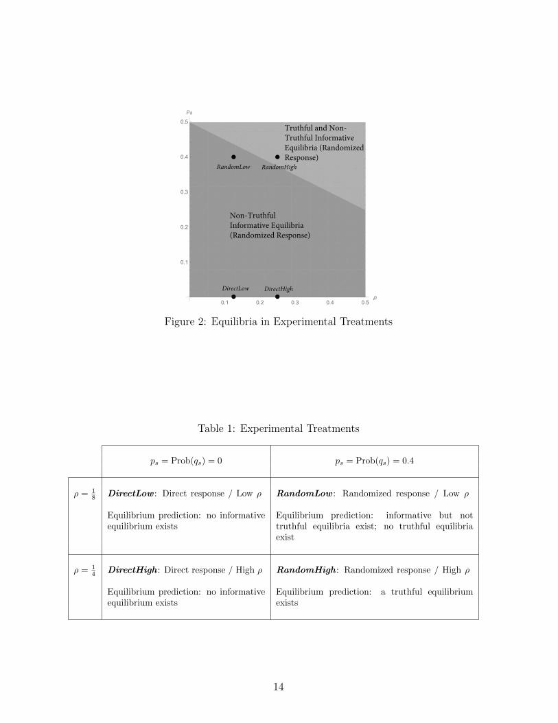
Recall that Figure 1 provided a graphical representation of our theoretical characteriza-

tion of the set of equilibria under randomized response. Figure 2 reproduces that portion

of Figure 1 where ρ < 12

(and therefore there is no communication possible under direct

response) and shows in addition the four parameter combinations used in our experiment.

Table 1 summarizes our 2×2 design and states the theoretical prediction for each treatment.

5.2 Hypotheses

Our experimental hypotheses derive from our characterization of the sets of equilibria under

direct and randomized response in Section 4, including the D1 criterion whenever it applies.

Taking a first, coarse, look at whether randomized response has the desired effects on

incentives to be truthful, we begin by comparing the behavior of the stigmatized type

(type s) under direct response and randomized response. Recall that for the parameters

7This also happens to be the range that is of greatest interest for practitioners. Randomized responseand similar techniques are intended to be used to gather information about sensitive issues and, all elseequal, the higher the sensitivity of the issue (which is represented by ξ in our model), the lower is ρ = λ

ξ .

13

0.1 0.2 0.3 0.4 0.5ρ

0.1

0.2

0.3

0.4

0.5

ps

Truthful and Non-Truthful Informative Equilibria (Randomized Response)

Non-Truthful Informative Equilibria (Randomized Response)

RandomLow RandomHigh

DirectLow DirectHigh

Figure 2: Equilibria in Experimental Treatments

Table 1: Experimental Treatments

ps = Prob(qs) = 0 ps = Prob(qs) = 0.4

ρ = 18 DirectLow : Direct response / Low ρ

Equilibrium prediction: no informativeequilibrium exists

RandomLow : Randomized response / Low ρ

Equilibrium prediction: informative but nottruthful equilibria exist; no truthful equilibriaexist

ρ = 14 DirectHigh : Direct response / High ρ

Equilibrium prediction: no informativeequilibrium exists

RandomHigh : Randomized response / High ρ

Equilibrium prediction: a truthful equilibriumexists

14

in our experiment according to Proposition 1 the stigmatized type always lies under direct

response. Proposition 2, in contrast, establishes that under randomized response there

are equilibria in which type s is truthful with positive probability. This gives us our first

hypothesis:

Hypothesis 1. Under randomized response stigmatized types are significantly more often

truthful than they are under direct response.

The second hypothesis examines the effects of randomized response on truth-telling

more closely. It is based on the recognition that in order for randomized response to be

effective, it is not enough that s types become more truthful. The key to randomized

response being successful is making senders more truthful when being truthful adversely

affects receiver’s beliefs from the sender’s perspective. This is what we have termed giving

“difficult truthful answers.”

In our setting, where qt is the more frequent question, in an informative equilibrium a

“yes” answer shifts the receiver’s belief toward placing more weight on the sender being type

t. Hence, an s type who is confronted with question qs has every reason to be truthful; she

earns a direct reward for being truthful and benefits from having beliefs move in the desired

direction. The more difficult situation for an s type arises when the question she is asked is

qt. In that case, if she truthfully answers “no” she induces beliefs that lower her payoff. For

s to answer qt with “no” is a difficult truthful answer; the same is true for t answering qs

with “no.” Without these “no” answers, the sender would always answer “yes” and thus no

information would be transmitted. Inducing difficult truthful answers is therefore the key

mechanism by which randomized response promises to improve information transmission.8

Proposition 1 shows that the sender never gives difficult truthful answers under direct

response. In contrast, Proposition 2 establishes that under randomized response there are

informative equilibria; this requires that senders give difficult truthful answers some of the

time.

Hypothesis 2. The proportion of senders who are truthful when this requires giving difficult

answers is significantly higher under randomized response than it is under direct response.

Hypothesis 2 is pivotal to the assessment of whether randomized response can improve

information transmission. If we were to reject it, randomized response would fail at the

most basic level.

8Recall that our discussion focuses on those non-truthful informative equilibria in which type θ = s, tis truthful when asked question qθ. The point made in this paragraph applies equally to the other non-truthful equilibria (in which θ = s, t is truthful when asked question q−θ), except that for those equilibria“yes” is the difficult answer, the answer that moves receiver beliefs in a direction unfavorable to the sender.

15

Our third hypothesis focuses on direct response. Theory predicts that there is no

difference in behavior between the two direct response treatments (Proposition 1). Both

types of the sender always answer with “yes” to the (commonly known) question “Are you

a t?” It is an empirical question whether this is the case; it could be, for example, that

due to homegrown truth-telling preferences there is more truth-telling in the lab than the

theory allows. This suggests the following hypothesis:

Hypothesis 3. There is no significant difference in behavior between DirectLow and Di-

rectHigh.

Our fourth hypothesis addresses a key property of randomized response. While theory

allows for informative equilibria with both high (ρ = 14) and low (ρ = 1

8) relative truth-

telling preferences, full truth-telling is (only) possible for ρ = 14

(Proposition 2). Theory

does not make a sharp prediction here since there is multiplicity of equilibria with ρ = 14,

but it is important to check whether randomized response realizes its full potential for high

relative truth-telling preferences. This motivates the following hypothesis.

Hypothesis 4. Senders are truthful under RandomHigh.

Our primary interest in this paper is in whether senders use more informative strategies

under randomized response than under direct response. Since those strategies, in equilib-

rium, need to be supported by appropriate receiver beliefs, it is worth examining those

beliefs. This is the topic of our fifth hypothesis. It is based on the following theoretical

considerations.

An equilibrium is informative if posterior beliefs differ from the prior for messages sent in

equilibrium. By the martingale property of Bayesian updating (the expectation of posterior

beliefs equals the prior belief), it follows in our case (Proposition 2) that beliefs following

“no” answers must differ from beliefs following “yes” answers in informative equilibria of

the randomized response treatments.9 This motivates Hypothesis 5.

Hypothesis 5. Elicited beliefs under randomized response differ depending on whether a

“yes” or a “no” answer is received.

Consistent with the theory, we do not hypothesize beyond the fact that the beliefs differ.

That said, equilibria with higher weight on s after a “no” answer appear more plausible,

given that that pattern obtains for both direct response equilibria and truthful randomized

response equilibria.

9In the direct response treatments, the D1 pooling equilibria from Proposition 1 predict that onlymessage “yes” is sent in equilibrium and hence the belief after “yes” is that s and t are equally likely,identical to the prior.

16

5.3 Design and Procedures

Our experiment was conducted at the Pittsburgh Experimental Economics Lab. A total

of 304 subjects with no prior experience in these experiments were recruited from the

undergraduate/graduate population of the University of Pittsburgh to participate in 16

experimental sessions, four per each treatment. A between-subject design was used, and

each session involved 16−20 distinct subjects making decisions in 8−10 randomly matched

groups.10 The experiment was programmed and conducted using z-Tree (Fischbacher [30]).

In each session, half the subjects were randomly assigned the role of Member A (sender)

and the other half the role of Member B (receiver), with role assignments remaining fixed

throughout the session. They participated in 40 rounds of decisions in groups of two.11

After each and every round, subjects were randomly rematched. In each group and each

round, the computer randomly drew either SQUARE (s) or TRIANGLE (t). Both members

were informed about the fact that each shape would have an equal chance to be drawn, but

the selected shape would be revealed only to Member A. In the direct response treatments,

Member A was presented with the question “Was TRIANGLE selected?” (qt), which was

known to Member B. In the randomized response treatments, the computer would draw a

question from either “Was SQUARE selected?” (qs) or “Was TRIANGLE selected?” Both

members were informed about the fact that the former question would have a 40% chance

to be drawn, but the selected question would be revealed only to Member A. In both sets of

treatments, Member A responded to the question being asked, either with “yes” or “no.”

The response was revealed to Member B, who was then asked to predict the likelihood

that SQUARE or TRIANGLE was drawn. Member B was asked to allocate 100 shapes

between SQUARE and TRIANGLE, where the number of SQUARES would represent the

predicted likelihood that SQUARE was selected.

We used monetary incentives to induce a preference for truth-telling (λ in the model)

and stigmatization aversion (ξ in the model). Subjects were rewarded in each round in

experimental currency units (ECU).12 If Member A’s answer to the question truthfully re-

10We set a recruiting target of 20 subjects (10 groups) for a session and set a minimum of 16 in case ofinsufficient show-ups. We met our target for 10 sessions, with the remaining six sessions four conductedwith 18 subjects and two conducted with 16 subjects.

11Before the 40 official rounds, subjects participated in 6 rounds of practice, in which they assumed therole of Member A for three rounds and Member B for another three rounds. The objective of subjectsassuming both roles in the practice rounds was to familiarize them with the computer interface and theflow of the whole decision process.

12We randomly selected three rounds and used the average earning in the selected rounds for realpayments at the exchange rate of 10 ECU for 1 USD. As will be discussed below, there was a rather largevariation in what a Member B could earn in a round. The use of three round average was intended tosmooth out the variations. Payments to subjects ranged from, including a $5 show-up fee, $10 to $35, withan average of $29.7.

17

vealed which shape was selected, he/she would receive 300 ECU in DirectHigh/RandomHigh

and 275 ECU in DirectLow/RandomLow ; with untruthful answers, he/she would receive

250 ECU. Therefore, depending on the treatment, there was a reward of either 50 ECU or

25 ECU for being truthful.

Stigmatization aversion was induced as follows: Member A’s ECU would be reduced

by twice the number of SQUARES allocated by Member B. Thus, compared to the case

where Member B assigned a probability of zero to SQUARE, Member A’s earning was 200

ECU lower than when Member B assigned a probability of one to SQUARE.

We implemented different levels of relative truth-telling preferences ρ = λξ

by varying λ.

In DirectLow and RandomLow ρ = λξ

= 18

was implemented as 25 ECU200 ECU

and in DirectHigh

and RandomHigh ρ = λξ

= 14

was implemented as 50 ECU200 ECU

.13

We incentivized Member B to report her/his beliefs truthfully. Under the belief-

elicitation mechanism that we employed, irrespective of risk attitudes, truthful reporting of

one’s beliefs is a dominant strategy (Karni [46]).14 In the following, we describe the essence

of our reward procedure that implements the mechanism; the details of the presentation to

subjects can be found in the sample experimental instructions in Appendix B.

The procedure used two binary lotteries. In both lotteries the outcomes were SQUARE

(with monetary payoff 300 ECU for Member B) and TRIANGLE (with monetary payoff

50 ECU for Member B). The probability of SQUARE in the first lottery was drawn from

a uniform distribution over the set{

0, 1100, 2

100, . . . , 99

100, 1}. The outcome SQUARE in the

second lottery was realized if the computer had chosen SQUARE for Member A’s type.

If the draw from the uniform distribution over{

0, 1100, 2

100, . . . , 99

100, 1}

resulted in a higher

value than Member B’s predicted likelihood of SQUARE having been selected for Member

A’s type, the first lottery was used to determine Member B’s payoffs. Otherwise, the second

lottery was used to determine Member B’s payoffs. Under this reward procedure, making

predictions according to true beliefs always guaranteed Member B a draw from the lottery

whose (subjective) probability of earning the higher “prize,” 300 ECU, was higher, thus

13This design approach was motivated by maintaining reasonable bounds on earnings that do not differby too much across treatments. The base earning of 250 ECU ensured, with the induced ξ = 200, thatsubjects received a minimum of 50 ECU in a round; subjects were thus guaranteed, excluding the show-upfee, a positive payment of $5. On the other hand, the maximum ECU that a subject could earn in a roundwas 275 − 300; subjects’ pre-show-up-fee payments were thus capped by $27.5 in DirectLow/RandomLowand $30 in DirectHigh/RandomHigh. Had we varied the absolute level of stigmatization aversion, we wouldhave had to adjust the base earning upward for DirectHigh and RandomHigh resulting in a considerablyhigher upper bound of payments or, with no such upward adjustment, accept the possibility of negativeearnings.

14Other efforts to attenuate biases caused by risk attitudes in belief elicitation include Allen [1], Offer-man, Sonnemans, van de Kuilen, and Wakker [59], Schlag and van der Weele [65] and Hossain and Okui[40].

18

providing the incentives for reporting true beliefs.15

At the end of each round, we provided information feedback on which shape was selected,

which question was selected (for randomized response), Member A’s answer, Member B’s

prediction, and the subject’s own earning.

6 Experimental Findings

6.1 Senders’ Answers and Receivers’ Beliefs

Our first result, illustrated in Figure 3, compares the randomized response and direct

response treatments with respect to the behavior of stigmatized types. Figure 3 presents

the trends of truthful answer frequencies by type. The left panel shows that stigmatized

types are more truthful under randomized response than under direct response.

0.00

0.20

0.40

0.60

0.80

1.00

1 3 5 7 9 11 13 15 17 19 21 23 25 27 29 31 33 35 37 39

Proportion

Round

Frequencies of Truthful Answers by s‐types

DirectLow DirectHigh RandomLow RandomHigh

(a) s-types

0.00

0.20

0.40

0.60

0.80

1.00

1 3 5 7 9 11 13 15 17 19 21 23 25 27 29 31 33 35 37 39

Proportion

Round

Frequencies of Truthful Answers by t‐types

DirectLow DirectHigh RandomLow RandomHigh

(b) t-types

Figure 3: Trends of Truthful Answer Frequencies

Result 1. Stigmatized types provided truthful answers more often in the randomized re-

sponse treatments than in the direct response treatments.

Result 1 confirms Hypothesis 1. The frequencies of truthful answers by s-types, ag-

gregated across the last 20 rounds of all sessions, were 19% in DirectLow and 37% in

DirectHigh. The corresponding frequencies were 79% in RandomLow and 89% in Ran-

domHigh. Using session-level data as independent observations, statistical tests confirm

that the frequencies are significantly higher in the randomized response treatments irre-

spective of the levels of relative truth-telling preferences (p = 0.0143 for all four possible

15Using induced beliefs, Hao and Houser [39] experimentally evaluate the mechanism in Karni [46]. Theway we presented the mechanism to the subjects was similar to theirs.

19

comparisons, Mann-Whitney tests).16

For t-types, the truthful answer frequencies were significantly lower in the randomized

response treatments, but in aggregate the magnitudes of the differences were at most one

third of those of s-types: the frequencies were 98% in both DirectLow and DirectHigh, 84%

in RandomLow, and 90% in RandomHigh (p = 0.0143 for all four possible comparisons,

Mann-Whitney tests).

The fact that t-types become less truthful under randomized response, while s-types

become more truthful, is consistent with the form non-truthful informative equilibria take

in the game we analyzed. Under randomized response being truthful requires accepted

types (t) sometimes to give what we have called “difficult answers,” answers that adversely

affect receiver’s beliefs. This is the case when t-types are asked question qs and to be

truthful have to answer with “no.” The intuition that accepted types may want to avoid

giving difficult truthful answers and instead engage in non-truthful protective behavior is

confirmed by both our formal analysis and our experimental data.

Our second, and central, result compares the behavior of senders under randomized and

direct response in situations when being truthful requires giving difficult answers. Figure

4 presents the aggregate frequencies of answers. The top panel shows the answers for the

direct response treatments, by type and question. The bottom panel shows the same for

randomized response. The frequency bars corresponding to difficult truthful answers are

circled in Figure 4. They show that difficult truthful answers are more frequent under

randomized response than under direct response.

Result 2. There was a significantly higher frequency of difficult truthful answers under

randomized response than under direct response.

Under direct response being truthful requires giving a difficult answer whenever the

sender’s type is s. The difficult truthful answer is “no.” Under randomized response being

truthful requires giving a difficult answer when either the sender’s type is s and the question

is qt or the sender’s type is t and the question is qs. Once again, the difficult truthful answer

is “no” in both cases. We therefore compare the frequencies of “no” answers in the event

that the type is s under direct response with the frequencies of “no” answers in the event

{(s, qt), (t, qs)} under randomized response (circled in Figure 4). The comparisons, which

16All aggregate data reported and used for statistical testings are from the last 20 rounds. The qualitativeaspects of our findings remain unchanged if we use, for example, data from the last 30 or even all 40rounds. However, the frequency trends, especially those for s-types in the direct response treatmentswhere convergence was most conspicuous, suggest that the 20th round provides a reasonable cutoff forbehavior having settled down. Using data from the last 20 rounds thus allows us to give more weight toconverged behavior. Unless otherwise indicated, the reported p-values are from one-sided tests.

20

0.00

0.20

0.40

0.60

0.80

1.00

yes no† yes† no

s t

Prop

ortio

n

Are you a t?Type‐Answer

Frequencies of Answers in Direct Response Treatments

DirectLow

DirectHigh

† truthful answers

(a) Direct Response Treatments

0.00

0.20

0.40

0.60

0.80

1.00

yes† no yes no† yes no† yes† no

s t s t

Are you an s? Are you a t?

Prop

ortio

n

Question‐Type‐Answer

Frequencies of Answers in Randomized Response Treatments

RandomLowRandomHigh

† truthful answers

(b) Randomized Response Treatments

Figure 4: Frequencies of Answers

involve comparing 19% in DirectLow with 67%/63% in RandomLow and 37% in DirectHigh

with 84%/78% in RandomHigh, confirm Hypothesis 2 (p = 0.0143 for all four comparisons,

Mann-Whitney tests).

Result 2 summarizes our most important finding in support of the mechanism that drives

randomized response. The key route by which randomized response promises to improve

information transmission is by facilitating the elicitation of difficult truthful answers. It

is a necessary condition for randomized response to be effective. Result 2 shows that

randomized response meets this bar.

This shows that in the present context garbling has the intended effects on incentives.

Because of garbling the receiver draws less extreme inferences from the sender’s message.

This relaxes incentive constrains of the sender, making it easier for the sender to transmit

at least some information.

Our third result concerns the direct response treatment. Behavior under direct response

is of interest, because if there is already significant information transmission under direct

response, there is less room for randomized response to improve on direct response. Given

21

our parameter choices, theory predicts that under direct response there is no information

transmission for both levels of relative truth-telling preferences, ρ = 14

and ρ = 18. Contrary

to theory we find that more information is transmitted for the higher level of relative

truth-telling preferences (ρ = 14). This is driven by stigmatized types being more truthful

than theory predicts, and being more truthful for higher induced relative truth-telling

preferences.

Result 3. Under direct response, stigmatized types provided truthful answer significantly

more often in the high relative truth-telling treatment (ρ = 14) than in the low relative

truth-telling treatment (ρ = 18).17

A detailed examination of the direct response data shows that the behavior of t-types

was very close to the point prediction of the D1 pooling equilibrium, where in both Di-

rectLow and DirectHigh the frequencies of “yes” were 98%. On the other hand, s-types

answered “yes” less often than did t-types, with frequencies 81% in DirectLow and 63% in

DirectHigh. Given that t-types almost always answered with “yes,” s-types’ non-negligible

uses of “no” transmitted information, in contrast to the prediction of the pooling equi-

librium. Over-communication, a common finding in the experimental literature of com-

munication games (e.g., Forsythe, Lundholm, and Rietz [32]; Blume, Dejong, Kim, and

Sprinkle [9], 2001; Cai and Wang [16]), was thus also observed in our experiments; unlike

in those games here over-communication is not accounted for by a level-k analysis and

more likely due to homegrown truth-telling preferences.18 We can reject Hypothesis 3 since

s-types over-communicated more for higher relative truth-telling preferences (p = 0.0286,

Mann-Whitney test), giving us Result 3 stated above.

Our fourth result deals with the question of whether randomized response lives up to

its full potential for promoting truth-telling. Theory indicates that complete truth-telling

is possible in RandomHigh (ρ = 14). Our experimental results, however, indicate that full

truth-telling is not achieved. This is summarized in the following result.

Result 4. Senders were significantly less truthful than theory would permit in RandomHigh.

The frequency of the senders (both types) being truthful was 90% in RandomHigh, im-

mediately rejecting Hypothesis 4 that senders are truthful. If we allow for some randomness

17To a lesser degree, accepted types provided truthful answer significantly more often in RandomHighthan in RandomLow ; there was no significant difference in accepted types’ truthful answer frequenciesbetween DirectLow and DirectHigh.

18We conducted an additional session for robustness check, where the parameters were the same asDirectHigh except that ps = 1 (i.e., the direct question became “Are you an s?”). Compared to DirectHighwith ps = 0, a higher instance of over-communication by s-types was observed: the frequency of truthful“yes” was 46%. There was almost no difference for t-types, where the frequency of truthful “no” was 99%.

22

in choices and only ask for senders being truthful at least 95% of the time, the hypothesis

is still rejected (p = 0.0625, Wilcoxon signed-rank test).19

The reason for this finding is that senders systematically deviated from truth-telling

when this required giving difficult answers. In the randomized response treatments, there

was a lower incidence of difficult truthful answers (“no”) than of truthful answers that were

not difficult (“yes”). In RandomHigh, for the question “Are you an s?” s-types answered

with “yes” with frequency 97%; for the question “Are you a t?” t-types answered with

“yes” with frequency higher than 99%. In contrast, for the question “Are you an s?”

t-types answered with “no” with frequency 78%; for the question “Are you a t?” s-types

answered with “no” with frequency 84%. The lower frequencies of difficult truthful answers

contributed to the rejection of Hypothesis 4. In fact, if we considered only the situations

in which being truthful requires giving difficult answers, we would reject the hypothesis

even more strongly; the frequency of the senders (both types) being truthful with difficult

answers was 82%, and the hypothesis is rejected even if we only ask for senders being

truthful at least 85% of the time (p = 0.0625, Wilcoxon signed-rank test).

Note also how truthful behavior changed with the change in relative truth-telling pref-

erences from RandomHigh to RandomLow. In RandomLow, for the question “Are you an

s?” s-types answered with “yes” with frequency 93%, and t-types answered with “no” with

frequency 63%; for the question “Are you a t?” t-types answered with “yes” with frequency

higher than 99%, and s-types answered with “no” with frequency 67%. The effects of lower

relative truth-telling preferences were again more pronounced with the difficult truthful

“no.”

The observed aggregate behavior is most consistent with non-truthful informative equi-

libria. In these equilibria the sender is truthful when this does not require giving a difficult

answer and otherwise fails to be truthful with positive probability: the frequencies of “yes”

answers by s-types to “Are you an s?” and by t-types to “Are you a t?” were close to

100% in both RandomHigh and RandomLow. In the cases where being truthful required

giving (difficult) “no” answers, the observed frequencies were within ±5% of the frequencies

generated by the mixing probabilities in non-truthful informative equilibria.20

It is instructive to reverse perspectives and try to determine which value of relative

19With four independent observations (sessions), p = 0.0625 is the lowest possible p-value for theWilcoxon signed-rank test.

20For µs(n) > µs(y), we have that σ(y|s, qs) = σ(y|t, qt) = 1, and the remaining equilibrium strategiessatisfy σ(n|t, qs) ∈ (0, 1) and σ(n|s, qt) = [

√25 + 80σ(n|t, qs) − 2σ(n|t, qs) − 5]/3 ∈ (0, 1] in RandomHigh

and σ(n|t, qs) ∈ (0, 1] and σ(n|s, qt) = [√

225 + 160σ(n|t, qs)− 2σ(n|t, qs)− 15]/3 ∈ (0, 1) in RandomLow.The formulae for equilibrium strategies can generate σ(n|s, qt) ≈ 0.89 (84% observed) and σ(n|t, qs) ≈ 0.73(78% observed) in RandomHigh and σ(n|s, qt) ≈ 0.63 (67% observed) and σ(n|t, qs) ≈ 0.67 (63% observed)in RandomLow.

23

truth-telling preference ρ is implied by the observed answer frequencies if one identifies

those frequencies with the mixing probabilities in a non-truthful informative equilibrium.

In the case of RandomHigh s-types answered qt with “yes” with a frequency of 16% and t-

types answered to qs with “yes” with a frequency of 22%. The implied relative truth-telling

preference ρ is approximately 0.2, compared to the induced ratio of 0.25. In the case of

RandomLow s-types answered qt with “yes” with a frequency of 33% and t-types answered

qs with “yes” with a frequency of 37%. The implied relative truth-telling preference is

approximately 0.17, compared to the induced ratio of 0.125. While those empirically implied

values are not exact matches for the ones we were trying to induce, they are in the right

range and preserve the order of the intended values. We take this calibration exercise

as further evidence that the informative non-truthful equilibria give a sensible account of

behavior in our randomized response treatments.21

The significantly lower frequencies of truthful “no” answers than theory says are possible

by accepted types represent the kind of protective behavior that John et al. [43] make

responsible for occasional non-intuitive data obtained with randomized response. Since in

our experiment “Are you a t?” is the more frequently asked question, in a putative truthful

equilibrium a “no” answer is difficult: “no” is the answer that moves posterior beliefs in the

direction of giving more weight to the stigmatized type. Thus t-types (as well as s-types),

all else equal, have an incentive to avoid giving “no” answers. In a truthful equilibrium this

incentive is balanced by the incentive to be truthful. As our equilibrium analysis reveals,

however, a complicating feature is that there are multiple equilibria and we therefore face

an equilibrium selection problem. It is not implausible that the balance of stigmatization

and truth-telling concerns also affects equilibrium selection; from this perspective the focal

principle of privacy protection may undermine that of truthfulness and push equilibrium

behavior away from the extreme of pure truth-telling.22

21One can also perform the calibration exercise for the direct response treatments. Consistent withthe over-communication we found there, the implied relative truth-telling preferences are markedly higherthan the induced ratios: in DirectHigh the implied relative truth-telling preference is 0.61, compared to aninduced value of 0.25; in DirectLow the implied relative truth-telling preference is 0.55, compared to aninduced value of 0.125. An interesting open question is how to reconcile the difference between the impliedvalues for direct response and randomized response. One possibility is that senders develop homegrownperceptions about ps. If they have an exaggerated sense of the difference between ps and pt, i.e., perceiveps to be lower than it is, the implied relative truth-telling preference increases. Another possibility isthat psychologically participants might not feel safe under randomized response, as John, Loewenstein,Acquisti, and Vosgerau [43] have suggested. Finally, it might be that truth-telling is more salient underdirect response since there is a more definite sense of what constitutes truth. The latter might be especiallyinteresting from an applied perspective, as it suggests a potentially adverse effect of randomized responseon truth-telling preferences.

22An additional contributing factor for observing protective behaviors in the field may be heterogeneityin individual weighting of truth-telling and stigmatization concerns. Those with stronger stigmatizationaversions might be expected to engage in protective behaviors even if others are content with being truthful.

24

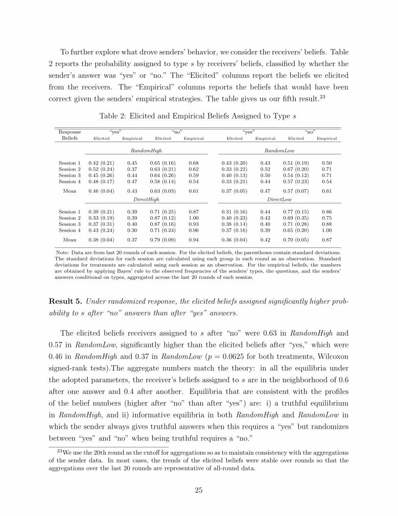
To further explore what drove senders’ behavior, we consider the receivers’ beliefs. Table

2 reports the probability assigned to type s by receivers’ beliefs, classified by whether the

sender’s answer was “yes” or “no.” The “Elicited” columns report the beliefs we elicited

from the receivers. The “Empirical” columns reports the beliefs that would have been

correct given the senders’ empirical strategies. The table gives us our fifth result.23

Table 2: Elicited and Empirical Beliefs Assigned to Type s

Response “yes” “no” “yes” “no”Beliefs Elicited Empirical Elicited Empirical Elicited Empirical Elicited Empirical

RandomHigh RandomLow

Session 1 0.42 (0.21) 0.45 0.65 (0.16) 0.68 0.43 (0.20) 0.43 0.51 (0.19) 0.50Session 2 0.52 (0.24) 0.37 0.63 (0.21) 0.62 0.33 (0.22) 0.52 0.67 (0.20) 0.71Session 3 0.45 (0.26) 0.44 0.64 (0.26) 0.59 0.40 (0.13) 0.50 0.54 (0.12) 0.71Session 4 0.48 (0.17) 0.47 0.58 (0.14) 0.54 0.33 (0.21) 0.44 0.57 (0.23) 0.54

Mean 0.46 (0.04) 0.43 0.63 (0.03) 0.61 0.37 (0.05) 0.47 0.57 (0.07) 0.61

DirectHigh DirectLow

Session 1 0.39 (0.21) 0.39 0.71 (0.25) 0.87 0.31 (0.16) 0.44 0.77 (0.15) 0.86Session 2 0.33 (0.19) 0.39 0.87 (0.12) 1.00 0.40 (0.23) 0.42 0.69 (0.35) 0.75Session 3 0.37 (0.31) 0.40 0.87 (0.16) 0.93 0.38 (0.14) 0.40 0.71 (0.28) 0.88Session 4 0.43 (0.24) 0.30 0.71 (0.24) 0.96 0.37 (0.16) 0.39 0.65 (0.20) 1.00

Mean 0.38 (0.04) 0.37 0.79 (0.09) 0.94 0.36 (0.04) 0.42 0.70 (0.05) 0.87

Note: Data are from last 20 rounds of each session. For the elicited beliefs, the parentheses contain standard deviations.The standard deviations for each session are calculated using each group in each round as an observation. Standarddeviations for treatments are calculated using each session as an observation. For the empirical beliefs, the numbersare obtained by applying Bayes’ rule to the observed frequencies of the senders’ types, the questions, and the senders’answers conditional on types, aggregated across the last 20 rounds of each session.

Result 5. Under randomized response, the elicited beliefs assigned significantly higher prob-

ability to s after “no” answers than after “yes” answers.

The elicited beliefs receivers assigned to s after “no” were 0.63 in RandomHigh and

0.57 in RandomLow, significantly higher than the elicited beliefs after “yes,” which were

0.46 in RandomHigh and 0.37 in RandomLow (p = 0.0625 for both treatments, Wilcoxon

signed-rank tests).The aggregate numbers match the theory: in all the equilibria under

the adopted parameters, the receiver’s beliefs assigned to s are in the neighborhood of 0.6

after one answer and 0.4 after another. Equilibria that are consistent with the profiles

of the belief numbers (higher after “no” than after “yes”) are: i) a truthful equilibrium

in RandomHigh, and ii) informative equilibria in both RandomHigh and RandomLow in

which the sender always gives truthful answers when this requires a “yes” but randomizes

between “yes” and “no” when being truthful requires a “no.”

23We use the 20th round as the cutoff for aggregations so as to maintain consistency with the aggregationsof the sender data. In most cases, the trends of the elicited beliefs were stable over rounds so that theaggregations over the last 20 rounds are representative of all-round data.

25

In the direct response treatments the receivers’ elicited beliefs were consistent with the

observed over-communication. While the D1 pooling equilibrium predicts that the receiver

believes s and t to be equally likely after receiving “yes,” the aggregate elicited beliefs

assigned to s were 0.38 in DirectHigh and 0.36 in DirectLow, significantly lower than 0.5

(p = 0.0625 for both treatments, Wilcoxon signed-rank tests). This did indicate that

receivers believed—correctly—that senders were transmitting information.

The out-of-equilibrium “no” was received, on average, 19% of the time in DirectHigh

and 10% of the time in DirectLow. The corresponding elicited beliefs assigned to s were

0.79 in DirectHigh and 0.70 in DirectLow, significantly higher than when “yes” was received

(p = 0.0625 for both treatments, Wilcoxon signed-rank tests). In fact, in DirectHigh 44% of

the time the elicited beliefs were equal to or larger than 0.9, while it was 31% in DirectLow.

Note that with higher probabilities assigned to s after “no” than after “yes,” answer-

ing with “yes” provided t-types with two monetary rewards, one from truth-telling and

one from inducing a lower probability assigned to s. This accounted for why t-types were

almost always truthful. On the other hand, when s-types told the truth with the diffi-

cult “no,” they were trading the truthful reward for a higher probability assigned to s.

Given the magnitudes of elicited beliefs, the latter on average was sufficient to outweigh

the former, suggesting that considerations other than monetary rewards might be driving

the over-communication observed in the direct response treatments.24 Prior experimental

studies have documented that subjects have intrinsic truth-telling preferences (e.g., Gneezy

[35]; Sanchez-Pages and Vorsatz [64]). In our case, it is conceivable that such homegrown

preferences were brought into the lab, which added on to our induced incentives, resulting

in a higher effective truth-telling preference. Indeed, the senders’ behavior in the direct

response treatments resembled the informative equilibrium under a higher value of ρ.25

6.2 Inference

While our primary interest is in information transmission, and not in inference, it is worth

briefly examining the impact of less-than-perfect truthfulness on inference.

24To support the uninformative equilibria, the out-of-equilibrium beliefs assigned to s were required tobe ≥ 0.75 in DirectHigh and ≥ 0.625 in DirectLow.

25Risk aversion might also have played a role. To avoid additional layers of complexity we did not usebinary lotteries (Roth and Malouf [63]; Berg, Dickhaut, and O’Brien [6]) to induce risk neutrality. Thesenders were trading a certain sum from truthful answers for a risky prospect of lower probability assignedto s. Given the variations in elicited beliefs, risk aversion might have favored truth-telling. Note, however,that this does not undermine the conclusion that the use of random questions led to more truth-telling, asvariations in elicited beliefs were also observed in the randomized response treatments; risk aversion waslargely controlled for in the comparisons between the two sets of treatments.

26

Table 3: Actual and Estimated Proportions of Stigmatized Types

Actual Estimated Actual Estimated

DirectHigh RandomHigh

Session 1 0.51 0.21 0.55 0.28Session 2 0.50 0.18 0.47 0.14Session 3 0.45 0.09 0.50 0.08Session 4 0.46 0.25 0.50 0.11

Mean 0.48 0.19 0.50 0.15

DirectLow RandomLow

Session 1 0.49 0.11 0.46 -0.45Session 2 0.44 0.04 0.59 -0.22Session 3 0.45 0.09 0.56 -0.58Session 4 0.50 0.17 0.48 0.08

Mean 0.47 0.10 0.52 -0.29

Note: Data are from last 20 rounds of each session. The means for treatments are calculated using each groupin each round as an observation.

One can easily verify that the departure from truth-telling in response to difficult ques-

tions, which is consistent with out theoretical analysis may result in distorted and even

invalid (negative) estimates of the proportion of stigmatized types in the population. This

concern is validated by our experimental data, as shown in Table 3. There we report for

each session the estimated prevalence of the stigmatized type in the population, using the

estimator proposed by Warner. We find that regardless of whether direct response or ran-

domized response is used, the estimated population proportion of the stigmatized type is

a underestimated. With lower relative truth-telling preferences, the estimated proportion

drops and in three out of four sessions with randomized response the estimate becomes

invalid. Thus basing inference on taking complete truth-telling for granted can be mislead-

ing.

6.3 Quantifying Information Transmission

One can use mutual information (see for example Cover and Thomas [23]) to quantify

how much information was transmitted in the lab under direct response and randomized

response.

The mutual information implied by our data is reported in Table 4. There we also report

a decomposition of the difference in mutual information between the direct response and

the randomized response treatments into i) the direct effect from randomizing questions,

which we refer to as “Noise,” ii) the protective strategic response by t-types to randomizing

questions—the avoidance of the difficult truthful “no” by t-types—which we refer to as

“Protective Behavior of t,” and iii) the primary intended strategic effect of randomized

27

response—to induce s-types to truthfully answer with “no” to the question “Are you a

t?”—which we refer to as the “Positive Effect of Randomized Response.”

Table 4: Mutual Information

DirectHigh Noise ProtectiveBehavior of t

Positive Effectof RandomizedResponse

Remaining RandomHigh

Session 1 0.134 0.039Session 2 0.213 0.046Session 3 0.080 0.017Session 4 0.267 0.003

Mean 0.173 −0.171 +0.012 +0.023 −0.011 0.026

DirectLow Noise ProtectiveBehavior of t

Positive Effectof randomizedresponse

Remaining RandomLow

Session 1 0.055 0.006Session 2 0.012 0.027Session 3 0.056 0.030Session 4 0.198 0.009

Mean 0.080 −0.076 +0.036 +0.007 −0.029 0.018

Note: The formula for mutual information is∑P (θ′, r′) log

P (θ′|r′)P (θ′) , where (θ′, r′) ∈ {s, t}×{y, n}. The figures are obtained

by applying the equivalent∑P (r′|θ′)P (θ′) log

P (r′|θ′)P (r′) to the empirical counterparts (last-20-round aggregates) of P (θ′),

P (qθ′ ), and P (r′|qθ′ , θ′). The effect of Noise is obtained by, starting with the mutual information under direct response,replacing P (qs) and P (qt) in direct response with those in randomized response. (In the same step, negation of the answerto qt is also used for the frequency of answers to the unasked question qs in direct response, i.e., we assume that for directresponse P (r′|qs, θ′) = 1 − P (r′|qt, θ′).) The effect of Protective Behavior of t is obtained by replacing P (r′|qs, t) in directresponse with those in randomized response. The Positive Effect of Randomized Response is obtained by replacing P (r′|qt, s)in direct response with those in randomized response. The remaining effect is obtained by replacing the remaining P (r′|·, ·)in direct response with those in randomized response.

Theory predicts that for the parameters in our experiment randomized response out-

performs direct response. Direct response, however, dominates in the lab due to over-

communication. While in the presence of such over-communication randomized response

does not improve information transmission over direct response in our data as measured

by the mutual information, it is important to remember that it does move truth-telling

behavior in the desired direction (Results 1 and 2). This suggests that the key mechanism

motivating the use of randomized response does work. This is confirmed by the decompo-

sition of the difference in the mutual information, which reveals that the strategic effects of

randomized response (“Positive Effect of Randomized Response” and “Protective Behavior

of t”) make a positive, though small, contribution to information transmission. The (seem-

ingly counterintuitive) positive sign of the “Protective Behavior of t” effect reflects the fact

that under direct response t-types have an even greater incentive to answer the (hypothet-

ical) question “Are you an s?” with“yes.” Thus “Protective Behavior of t” is diminished

under randomized response, which has a positive effect on information transmission.

28

7 Related Literature

Plausible deniability may be used to deflect responsibility26, distort information27, and can

reduce incentives for pro-social behavior.28 On the positive side, it may provide protection

for whistleblowers (Chassang and Padro i Miquel [18]) and make it possible to communicate

useful first-order information while withholding damaging higher-order information (Ayres

and Nalebuff [2]). From a design perspective, a natural question then is how to balance

the benefits of plausible deniability, e.g., from privacy protection, with its costs, e.g., from

contamination of information channels.

The literature has studied a range of devices that can generate plausible deniability,

such as restrictions on ex post information about behavior (Tadelis [69]; Dana et al. [28]),

indirect or ambiguous language (Ayres and Nalebuff [2]; Pinker, Nowak, and Lee [62];

Mialon and Mialon [55]) and commitment to random intervention (Chassang and Padro

i Miquel, [18]). Recent theoretical work on noisy communication channels (Blume et al.

[10]), non-strategic mediators (Goltsman et al. [38]), strategic mediators (Ivanov [42]) and

stochastic continuations (Krishna and Morgan [51]) in variants of the Crawford and Sobel

[24] model can also be viewed in this vein.

This potential of randomness providing plausible deniability was first recognized by

Warner [71]. There is by now a large number of variations on Warner’s original technique.

In the innocuous question technique, the second question is replaced by an unrelated ques-

tion such as “Have you ever visited a local library?” Another version that is widely used

in the survey design literature (e.g., St John et al. [67]) is the forced response technique

proposed by Boruch [14]. With this approach, depending on realization of the randomizing

device, participants are instructed to either answer a sensitive question or to give a pre-

scribed response irrespective of the truth (e.g., always answer “yes”). In the item count

technique (also known as the list response technique) proposed by Miller [56], participants

are asked to report how many of N + 1 items are true when among them only one item is

sensitive (see, e.g., Karlan and Zinman [45] with an application to measuring the use of mi-

cro finance loan proceeds, and Coffman, Coffman, and Ericson [22] on LGBT populations).

26An example is Admiral John Poindexter’s assumption of responsibility for the diversion of some of theproceeds from arms sales to Iran to support the Contras in Nicaragua and his withholding of documentsfrom President Reagan to provide him with deniability (Bogen and Lynch [13]).

27Calomiris [17] notes that in the case of novel financial instruments the lack of a track record is a sourceof deniability for rating agencies with an interest in rating inflation.

28Tadelis [69] reports data from a trust-game experiment in which trustees returned less when theirdecisions could not be distinguished from random events. Dana, Cain, and Dawes [28] find that subjectsfrequently are willing to avoid playing a $10 dictator game in favor of a $9 exit option, when using the exitoption ensures that the (potential) receiving player does not learn that otherwise a dictator game wouldhave been played.

29

Variants of the randomized response technique have been used to gather information about

a large variety of sensitive issues, including drug use and doping (Striegel, Ulrich, and

Simon [68]), tax evasion (Houston and Tran [41]), employee theft (Wimbush and Dalton

[72]), poaching (St John et al. [67]), regulatory non-compliance (Elffers, van der Heijden,

and Hezemans [29] and the integrity of certified public accountants (Buchman and Tracy

[15]).

The use of randomized response is predicated on randomization inducing truth-telling.

For this to be the case, there must be at least some preference for truth-telling to outweigh

privacy concerns; senders must appropriately process the inference-moderating effect of

randomness; and, if the game that is induced between the sender and the receiver has

multiple equilibria, then a truth-telling one must be selected.

Thus far, efforts to evaluate whether randomized response works as predicted, rather

than examining the above conditions, have primarily focused on two empirical validation

methods, individual validation and comparative validation. The former relies on the rare

instances when there is direct evidence on the empirical question of interest that can be con-

trasted with the results from a randomized response study. The latter compares data from

randomized response studies with those from alternative survey methods (self-administered

questionnaires, telephone interviews, face-to-face interviews, and computer-assisted inter-

views). Examples of comparative validation studies are Beldt, Daniel, and Garcha [5],

Wimbush and Dalton [72], and Lensvelt-Mulders, Hox, van der Heijden, and Maas [52].

Their results suggest that randomized response improves on direct questioning according

to the more-is-better criterion, where a higher population estimate of the stigmatized trait

is interpreted as being more valid.

Recently, and independently, John et al. [43] have conducted experiments to evaluate

randomized response. They are motivated by empirical findings according to which there

is frequent non-adherence to randomized response instructions, direct response often yields

more valid responses than randomized response, and sometimes randomized response gen-

erates invalid prevalence estimates. They suggest that those “paradoxical findings” might

be rooted in either unclear instructions or “protective behavior” of participants who worry

that innocuous responses are viewed as admissions. Consistent with those rationales they

find that non-adherence to randomized response instructions can be alleviated and esti-

mates improved by framing jeopardizing responses as socially desirable and by clarifying

that jeopardizing responses do not amount to admissions.

We also provide experimental evidence for systematic non-adherence to randomized

response instructions. Consistent with the prior evidence cited by John et al. [43], in

our data randomized response systemically underestimates the population proportion of

30

the stigmatized trait, and when relative truth-telling preferences are low we get negative

and thus invalid estimates. We experimentally demonstrate that non-adherence can be

explained by protective behavior and that protective behavior becomes more pronounced

with increasing concerns about stigmatization relative to truth-telling incentives.

8 Discussion and Conclusion

The principal insight from our theoretical analysis of the randomized response game is that

there are informative equilibria that are not truthful. Behavior in line with those equilibria

can imply distorted and possibly invalid estimates of the prevalence of the stigmatized trait

in the population. Furthermore, they plausibly express the focal principle of privacy pro-

tection. Therefore, there is no need for auxiliary explanations of observed non-compliance

with randomized response instructions. Non-truthful behavior is rational and varies in a

predictable fashion with incentives.

Our experimental findings are best accounted for by informative but non-truthful equi-

libria. Consistent with these equilibria, randomized response improves truth-telling by

stigmatized types (Result 1) and, importantly, increases the frequency of difficult truthful

answers (Result 2). Thus the fundamental mechanism that underpins the rationale for

randomized response does work.

At the same time, we find systematic departures from truth-telling with difficult an-

swers. We find over-communication with direct response. With randomized response,

however, we find under-communication. Departures from truth-telling under randomized

response tend to be rational, occur for difficult answers, and vary with changing incentives.

One might wish to mitigate this effect by designing randomized response so that it

minimally moves posterior beliefs. Since this requires increasing the noise level it will have

to be accompanied by increasing sample size. In future work, it might be worthwhile using

laboratory experiments to investigate whether it is indeed the case that behavior becomes

approximately truthful when truthful answers to randomized questions are made nearly

uninformative; in our version of randomized response this would correspond to letting the

probability of asking each question converge to one half.

Another way to deal with the departures from complete truth-telling under randomized

response is to incorporate some recognition of non-truthfulness into the data analysis. This

has been advocated by Clark and Desharnais [21] and Cruyff, van den Hout, van der Heijden

and Bockenholt [27]. Experiments like ours can provide insights into the extent and nature

of the departures from complete truth-telling.

31

References

[1] Allen, Franklin [1987], “Discovering Personal Probabilities When Utility Functions

are Unknown,” Management Science 33, 452-454.

[2] Ayres, Ian and Barry Nalebuff [1996], “Common Knowledge as a Barrier to

Negotiation,” UCLA Law Review 44, 1631-1659.

[3] Banks, Jeffrey S., and Joel Sobel [1987], “Equilibrium Selection in Signaling

Games,” Econometrica 55 647–661.

[4] Battigalli, Pierpaolo, and Martin Dufwenberg [2009], “Dynamic Psycho-

logical Games,” Journal of Economic Theory bf 144, 1-35.

[5] Beldt, Sandra F., Wayne W. Daniel, and Bikramjit S. Garcha [1982], “The

Takahasi-Sakasegawa Randomized Response Technique: A Field Test,” Sociological

Methods & Research 11, 101-111.

[6] Berg, J. E., L. Daley, J. Dickhaut, and J. O’Brien [1986], “Controlling

Preferences for Lotteries on Units of Experimental Exchange,” Quarterly Journal of

Economics 101, 281-306.

[7] Bernheim, B. Douglas [1994], “A Theory of Conformity,” Journal of Political

Economy 102, 841-877.

[8] Bester, Helmut, and Roland Strausz [2007], “Contracting with imperfect com-

mitment and noisy communication,” Journal of Economic Theory 136, 236-259.

[9] Blume, Andreas, Douglas V. Dejong, Yong-Gwan Kim, and Geoffrey

B. Sprinkle [2001], “Evolution of Communication with Partial Common Interest,”

Games and Economic Behavior 37, 79-120.

[10] Blume, Andreas, Oliver J. Board, and Kohei Kawamura [2007], “Noisy

Talk,” Theoretical Economics 2, 395-440.

[11] Blume, Andreas and Oliver J. Board [2010], “Language Barriers,” University

of Pittsburgh Working Paper.

[12] Blume, Andreas and Oliver J. Board [2014], “Intentional Vagueness,” Erken-

ntnis 79, 855-899.

32

[13] Bogen, David and Michael Lynch [1989], “Taking Account of the Hostile Native:

Plausible Deniability and the Production of Conventional History in the Iran-Contra

Hearings,” Social Problems 36, 197-224

[14] Boruch, Robert F. [1972], “Strategies for Eliciting and Merging Confidential Social

Research Data,” Policy Sciences 3, 275-297.

[15] Buchman, Thomas A., and John A. Tracy [1982], “Obtaining Responses to

Sensitive Questions: Conventional Questionnaire versus Randomized Response Tech-

nique,” Journal of Accounting Research 20, 263-271.

[16] Cai, Hongbin, and Joseph Tao-Yi Wang [2006] “Overcommunication in Strategic

Information Transmission Games,” Games and Economic Behavior 56, 7-36.

[17] Calomiris, Charles W. [2009] “The Debasement of Ratings: What’s Wrong and

How We Can Fix It.” Columbia University Working Paper.

[18] Chassang, Sylvain, and Gerard Padro i Miquel [2013], “Corruption, Intimida-

tion and Whistleblowing: A Theory of Inference from Unverifiable Reports,” Princeton

University Working Paper.

[19] Chen, Ying [2011], “Perturbed Communication Games with Honest Senders and

Naive receivers,” Journal of Economic Theory 146, 401–424.

[20] Cho, In-Koo, and David Kreps [1987], “Signaling Games and Stable Equilibria,”

Quarterly Journal of Economics 102, 179-221.

[21] Clark, Stephen J., and Robert A. Desharnais [1998], “Honest answers to

embarrassing questions: Detecting cheating in the randomized response model.” Psy-

chological Methods 3, 160-168.

[22] Coffman, Katherine B., Lucas C. Coffman, and Keith M Marzilli Er-

icson [2013], “The Size of the LGBT Population and the Magnitude of Anti-Gay

Sentiment are Substantially Underestimated.” Ohio State University Working Paper.

[23] Cover, Thomas M., and Joy A. Thomas [1991], Elements of Information Theory,

John Wiley and Sons: New York, NY.

[24] Crawford, Vincent, and Joel Sobel [1982] “Strategic Information Transmis-

sion,” Econometrica 50, 1431-1451.

33

[25] Crawford, Vincent P. [2003], “Lying for Strategic Advantage: Rational and

Boundedly Rational Misrepresentation of Intentions,” American Economic Review 93,

133-149.

[26] Crawford, Vincent P., Miguel A. Costa-Gomes, and Nagore Iriberri

[2013], “Structural Models of Nonequilibrium Strategic Thinking: Theory, Evidence,

and Applications,” Journal of Economic Literature 51, 5-62.

[27] Cruyff, Maarten J.L.F., Ardo van den Hout, Peter G.M. van der Heij-

den, and Ulf Bockenholt [2007], “Log-linear randomized-response models taking

self-protective response behavior into account.” Sociological Methods & Research 36,

266-282.

[28] Dana, Jason, Daylian M. Cain, and Robyn Dawes [2006] “What You Don’t

Know Won’t Hurt Me: Costly (but Quiet) Exit in Dictator Games,” Organizational

Behavior and Human Decision Processes 100, 193-201.

[29] Elffers, Henk, Peter van der Heijden, and Merlijn Hezemans [2003] “Ex-

plaining Regulatory Non-Compliance: A Survey Study of Rule Transgression for Two

Dutch Instrumental Laws, Applying the Randomized Response Method,” Journal of

Quantitative Criminology 19, 409-439.

[30] Fischbacher, Urs [2007], “z-Tree: Zurich Toolbox for Ready-made Economic Ex-

periments,” Experimental Economics 10, 171-178.

[31] Forges, Francoise [1986], “An Approach to Communication Equilibria,” Econo-

metrica 54, 1375–1385.

[32] Forsythe, Robert, Russell Lundholm, and Thomas Rietz [1999], “Cheap

Talk, Fraud and Adverse Selection in Financial Markets: Some Experimental Evi-

dence,” Review of Financial Studies 12, 481-518.

[33] Frankel, Alex, and Navin Kartik [2017], “Muddled Information,” Journal of

Political Economy, forthcoming.

[34] Geanakoplos, John, David Pearce, and Ennio Stacchetti [1989] “Psycho-

logical Games and Sequential Rationality,” Games and Economic Behavior 1, 60-79.

[35] Gneezy, Uri [2005], “Deception: The Role of Consequences.” American Economic

Review 95: 384–394.

34

[36] Gingerich, Daniel W. [2010], “Understanding Off-The-Books Politics: Conduct-

ing Inference on the Determinants of Sensitive Behavior with Randomized Response

Surveys.” Political Analysis 18: 349–380.

[37] Giovannoni, Francesco, and Siyang Xiong [2017], “Communication under Lan-

guage Barriers,” University of Bristol Working Paper.

[38] Goltsman, Maria, Johannes Horner, Gregory Pavlov, and Francesco

Squintani [2009], “Mediation, Arbitration and Negotiation.” Journal of Economic

Theory 144, 1397-1420.

[39] Hao, Li, and Daniel Houser [2012], “Belief Elicitation in the Presence of Naive

Participants: An Experimental Study,” Journal of Risk and Uncertainty 44, 161-180.

[40] Hossain, Tanjim, and Okui Ryo [2013], “The Binarized Scoring Rule of Belief

Elicitation,” Review of Economic Studies 80, 984-1001.

[41] Houston, Jodie, and Alfred Tran [2001] “A Survey of Tax Evasion using the

Randomized Response Technique,” Advances in taxation 13, 69-94.

[42] Ivanov, Maxim [2010], “Communication via a Strategic Mediator,” Journal of Eco-

nomic Theory 145, 869-884.

[43] John Leslie K., George Loewenstein, Alessandro Acquisti, and Joachim

Vosgerau [2013], “Paradoxical Effects of Randomized Response Techniques,”

Carnegie Mellon University Working Paper.

[44] Kanodia, Chandra, Rajdeep Singh, and Andrew E. Spero [2005], “Impreci-

sion in accounting measurement: Can it be value enhancing?” Journal of Accounting

Research 43, 487–519.

[45] Karlan, Dean S., and Jonathan Zinman [2012], “List randomization for sensitive

behavior: An application for measuring use of loan proceeds.” Journal of Development

Economics 98, 71-75.

[46] Karni, Edi [2009], “A Mechanism for Eliciting Probabilities,” Econometrica 77, 603-

606.

[47] Kartik, Navin, Marco Ottaviani, and Francesco Squintani [2007],

“Credulity, Lies, and Costly Talk,” Journal of Economic Theory 134, 93–116.

35

[48] Kartik, Navin [2009], “Strategic Communication with Lying Costs,” The Review of

Economic Studies 76, 1359–1395.

[49] Kawamura, Kohei [2013] “Eliciting information from a large population,” Journal

of Public Economics 103, 44-54.

[50] Kaya, Ayca [2009], “Repeated Signaling Games” Games and Economic Behavior

66, 841–854.

[51] Krishna, Vijay, and John Morgan [2004], “The Art of Conversation: Eliciting

Information from Experts through Multi-Stage Communication,” Journal of Economic

Theory 117 147-179.

[52] Lensvelt-Mulders, Gerty J. L. M., Joop J. Hox, Peter G. M. van der

Heijden, and Cora J. M. Maas [2005], “Meta-Analysis of Randomized Response

Research: Thirty-Five Years of Validation,” Sociological Methods Research 33, 319-

348.

[53] Ljungqvist, Lars [1993], “A Unified Approach to Measures of Privacy in Random-

ized Response Models: A Utilitarian Perspective,” Journal of the American Statistical

Association 88, 97-103.

[54] Matthews, Steven A., and Leonard J. Mirman [1983], “Equilibrium Limit

Pricing: The Effects of Private Information and Stochastic Demand,” Econometrica

51, 981–996.

[55] Mialon, Hugo M., and Sue H. Mialon [2013], “Go Figure: The Strategy of

Nonliteral Speech,” American Economic Journal: Microeconomics 5, 186-212.

[56] Miller, JD. [1984] “A new survey technique for studying deviant behavior.” PhD

Dissertation, George Washington University.

[57] Mitusch, Kay, and Roland Strausz [2005], “Mediation in situations of conflict

and limited commitment,” Journal of Law, Economics, and Organization 21, 467–500.

[58] Myerson, Roger B. [1986], “Multistage Games with Communication,” Economet-

rica 54, 323–358.

[59] Offerman, Theo, Joep Sonnemans, Gijs van de Kuilen, and Peter P.

Wakker [2009], “A Truth-Serum for Non-Bayesians: Correcting Proper Scoring Rules

for Risk Attitudes,” Review of Economic Studies 76, 1461-1489.

36

[60] Ottaviani, Marco, and Peter Sørensen [2001], “Information Aggregation in

Debate: Who Should Speak First?,” Journal of Public Economics 81, 393–421.

[61] Ottaviani, Marco, and Peter Norman Sørensen [2006], “Reputational Cheap

Talk,” Rand Journal of Economics 37, 155-175.

[62] Pinker, Steven, Martin A. Nowak, and James J. Lee [2008], “The Logic of

Indirect Speech,” Proceedings of the National Academy of Sciences 105, 833-838.

[63] Roth, Alvin, and M. Malouf [1979], “Game-Theoretic Models and the Role of

Bargaining,” Psychological Review 86, 574-594.

[64] Sanchez-Pages, Santiago, and Marc Vorsatz [2007], “An Experimental Study

of truthful-responding in Sender-Receiver Game,” Games and Economic Behavior 61,

86-112.

[65] Schlag, Karl H., and Joel van der Weele [2009], “Efficient Interval Scoring

Rules,” Working Paper, Universitat Pompeu Fabra.

[66] Smith, Vernon L. [1976], “Experimental Economics: Induced Value Theory,” Amer-

ican Economic Review 66, 274-79.

[67] St John, Freya A. V. , Aidan M. Keane, Gareth Edwards-Jones, Lau-

ren Jones, Richard W. Yarnell, and Julia P. G. Jones [2012], “Identifying

Indicators of Illegal Behaviour: Carnivore Killing in Human-Managed landscapes.”

Proceedings of the Royal Society B, Biological Sciences 279, 804812.

[68] Striegel, Heiko, Rolf Ulrich, and Perikles Simon [2010], “Randomized Re-

sponse Estimates for Doping and Illicit Drug Use in Elite Athletes.” Drug and Alcohol

Dependence 106, 230-232.

[69] Tadelis, Steven [2011], “The Power of Shame and the Rationality of Trust.” UC

Berkeley Working Paper.

[70] Wang, Joseph Tao-yi, Michael Spezio, and Colin F. Camerer [2010],

“Pinocchio’s Pupil: Using Eyetracking and Pupil Dilation to Understand Truth Telling

and Deception in Sender-Receiver Games,” American Economic Review 100, 984-

1007.

[71] Warner, Stanley L. [1965], “Randomized Response: A Survey Technique for Elim-

inating Evasive Answer Bias,” Journal of the American Statistical Association 60,

63-69.

37

[72] Wimbush, Dan C., and Donald R. Dalton [1997] “Base Rate for Employee

Theft: Convergence of Multiple Methods,” Journal of Applied Psychology 82, 756-63.

38

Appendix A – Proofs

The following payoff profiles will be used in the proofs of Propositions 1 and 2.

U(s, qs, y, µs(y)) = U(t, qt, y, µs(y)) = ρ− µs(y), (A.1)

U(s, qs, n, µs(n)) = U(t, qt, n, µs(n)) = −µs(n), (A.2)

U(s, qt, n, µs(n)) = U(t, qs, n, µs(n)) = ρ− µs(n), (A.3)

U(s, qt, y, µs(y)) = U(t, qs, y, µs(y)) = −µs(y). (A.4)

Proof of Proposition 1. We characterize all equilibria under direct response where ps =

0. The fact that there exists no truthful equilibrium for ρ ∈ (0, 1) follows immediately from

constraint (1) in the main text, ρ ≥ 1− 2ps.

Note that in any informative equilibrium with ps = 0, we must have that µs(n) > µs(y);

if µs(y) > µs(n), it follows from (A.3) and (A.4) that s strictly prefers to send n, which

implies that µs(n) ≥ µs(y), a contradiction. With µs(n) > µs(y), it follows from (A.1) and

(A.2) that t strictly prefers to send y. Thus, in any informative equilibrium, t must send

truthful y with probability one and s must randomize between y and n. The indifference of s

between y and n implies, from (A.3) and (A.4), that ρ = µs(n)−µs(y). Given that n is used

exclusively by s, we have µs(y) = 1− ρ, which holds if and only if σ(n|s) = 2− 1ρ. Hence,

if an informative equilibrium exists, it is unique. The requirement that σ(n|s) ∈ (0, 1)

imposes the restriction that ρ > 12. Thus, if ρ ∈ (1

2, 1), one can construct an informative

equilibrium; if an informative equilibrium exists, we must have ρ ∈ (12, 1).

In any uninformative equilibrium, either i) only one message is used in equilibrium, or

ii) both messages are used and µs(y) = µs(n) = 12. Case ii) requires that σ(y|s) = σ(y|t) ∈

(0, 1), i.e., both s and t are indifferent between y and n, which can never hold given that

ρ > 0. Thus, case i) is the only possible form of any uninformative equilibrium. Suppose

that both s and t send y with probability one so that µs(y) = 12

on the equilibrium path. For

this to constitute an equilibrium, we require, from (A.1) and (A.2), that ρ ≥ 12− µs(n) for

t and, from (A.3) and (A.4), that µs(n)− 12≥ ρ for s, where µs(n) is an out-of-equilibrium

belief. Only the second inequality binds, and thus the out-of-equilibrium belief required to

support the equilibrium is that µs(n) ≥ ρ + 12. That µs(n) ∈ [0, 1] imposes the restriction

that ρ ≤ 12. Suppose next that both s and t send n with probability one so that µs(n) = 1

2

on the equilibrium path. By a similar argument, we require that the out-of-equilibrium

belief µs(y) ≥ ρ + 12, which again imposes the restriction that ρ ≤ 1

2. Thus, if ρ ∈ (0, 1

2],

one can construct uninformative equilibria with outcomes where either both types send y

or both send n, and these are the only uninformative equilibrium outcomes. Conversely, if

39

an uninformative equilibrium exists, we must have ρ ∈ (0, 12]. This also implies that for any

ρ ∈ (12, 1) there is no uninformative equilibrium, and hence in that range the informative

equilibrium is the only equilibrium.

We next apply the D1 criterion to the two equilibrium outcomes in which only one

answer is sent. Let U∗(θ) be the equilibrium payoff of type-θ sender. For the equilibrium

outcome in which both types send n, we have that U∗(s) = ρ − 12

and U∗(t) = −12.

If types s and t deviate to y, their payoffs will be, respectively, Ude(s) = −µs(y) and

Ude(t) = ρ−µs(y). Note that Ude(s)− U∗(s) ≥ 0, i.e., type s weakly prefers deviating to y,

if and only if µs(y) ∈ [0, 12− ρ]. On the other hand, Ude(t)− U∗(t) > 0, i.e., type t strictly

prefers deviating to y, if and only if µs(y) ∈ [0, 12

+ ρ). For ρ > 0, [0, 12− ρ] ⊂ [0, 1

2+ ρ); s

is deleted for y under the D1 criterion, and thus the equilibrium outcome does not survive

the selection criterion. Turning to the equilibrium outcome in which both types send y,

we note that type t weakly prefers deviating to n if and only if µs(n) ∈ [0, 12− ρ] and type

s strictly prefers deviating to n if and only if µs(n) ∈ [0, 12

+ ρ). By a similar argument,

the D1 criterion deletes t for n. The equilibrium outcome with both types sending y can

be supported by the resulting belief that µs(n) = 1; the outcome thus survives the D1

criterion.

Proof of Proposition 2. We establish the result by verifying the following claim, which

characterizes all equilibria under randomized response:

Under randomized response where ps ∈ (0, 12),

1. there exist uninformative equilibria if and only if ρ ∈ (0, 12];

2. there exists a truthful equilibrium if and only if ps ≥ 1−ρ2

; and,

3. the set of non-truthful informative equilibria is completely described by the following

statements:

(a) there exists an informative equilibrium in which (s, qs) and (t, qt) always give a

truthful answer and

i. (s, qt) always gives a truthful answer and (t, qs) randomizes between y and

n if and only if 1−ρ2< ps <

1ρ− 1;

ii. (s, qt) randomizes between y and n and (t, qs) always gives a truthful answer

if and only if ps <1−ρ

2;

iii. (s, qt) randomizes between y and n and (t, qs) always gives a non-truthful

answer if and only if ps <1ρ− 1 < 1

2;

40

iv. (s, qt) always give a truthful answer and (t, qs) always gives a non-truthful

answer if and only if ps = 1ρ− 1;

v. (s, qt) and (t, qs) randomize between y and n if and only if ps <1ρ− 1;

(b) there exists an informative equilibrium in which (s, qt) and (t, qs) always give a

truthful answer and

i. (s, qs) always gives a truthful answer and (t, qt) randomizes between y and

n if and only if ps > 2− 1ρ;

ii. (s, qs) randomizes between y and n and (t, qt) always gives a non-truthful

answer if and only if ps > 2− 1ρ> 0;

iii. (s, qs) always gives a truthful answer and (t, qt) always gives a non-truthful

answer if and only if ps = 2− 1ρ;

iv. (s, qs) and (t, qt) randomize between y and n if and only if ps > 2− 1ρ.

Given that the sender has four types, (s, qs), (t, qt), (s, qt) and (t, qs) and each type

can either answer with y with probability one, answer with n with probability one, or

completely randomize between y and n, there are in total 81 classes of strategy profiles as

candidates for equilibrium. We proceed by either characterizing the condition under which

a class of strategy profiles constitutes equilibria or eliminating a class as equilibrium, until

we exhaust all 81 possibilities.

We begin with the uninformative equilibria in Part 1 of the claim. In any such equi-

librium, either i) only one answer is used in equilibrium, or ii) both answers are used and

µs(y) = µs(n) = 12. Case ii) requires that σ(y|s, qs) = σ(y|t, qt) = σ(y|s, qt) = σ(y|t, qs) ∈

(0, 1), i.e., all types are indifferent between y and n, which can never hold given that ρ > 0.

One candidate for equilibrium is eliminated, leaving us with 80 possiblities. For case i),

consider first that all types answer with y with probability one so that µs(y) = 12

on the

equilibrium path. For this to constitute an equilibrium, we require, from (A.1) and (A.2),

that ρ ≥ 12− µs(n) for (s, qs) and (t, qt) and, from (A.3) and (A.4), that µs(n)− 1

2≥ ρ for

(s, qt) and (t, qs), where µs(n) is an out-of-equilibrium belief. Only the second inequality

binds, and thus the out-of-equilibrium belief required to support the equilibrium is that

µs(n) ≥ ρ + 12. That µs(n) ∈ [0, 1] imposes the restriction that ρ ≤ 1

2. Consider next that

all types answer with n with probability one so that µs(n) = 12

on the equilibrium path. By

a similar argument, we require that the out-of-equilibrium belief µs(y) ≥ ρ+ 12, which again

imposes the restriction that ρ ≤ 12. Thus, if ρ ∈ (0, 1

2], one can construct uninformative

equilibria where either all types answer with y or all types answer with n, and these are

the only uninformative equilibria. Conversely, if an uninformative equilibrium exists, we

must have ρ ∈ (0, 12].

41

We are left with 78 possibilities. We proceed to eliminate candidates for informative

equilibria, in which y and n are used with positive probability and µs(y) 6= µs(n). If

µs(n) > µs(y), it follows from (A.1) and (A.2) that (s, qs) and (t, qt) strictly prefer y and

thus σ(y|s, qs) = σ(y|t, qt) = 1. Similarly, if µs(y) > µs(n), it follows from (A.3) and

(A.4) that σ(y|s, qt) = σ(y|t, qs) = 0. The condition that either σ(y|s, qs) = σ(y|t, qt) = 1

or σ(y|s, qt) = σ(y|t, qs) = 0 eliminates 63 classes of strategy profiles, leaving 15 distinct

possibilities. Consider that µs(n) > µs(y) so that σ(y|s, qs) = σ(y|t, qt) = 1. The receiver’s

beliefs are

µs(n) =(1− ps)(1− σ(y|s, qt))

ps(1− σ(y|t, qs)) + (1− ps)(1− σ(y|s, qt)), (A.5)

µs(y) =ps + (1− ps)σ(y|s, qt)

1 + psσ(y|t, qs) + (1− ps)σ(y|s, qt). (A.6)

If σ(y|s, qt) = 1, both (s, qs) and (s, qt) answer with y with probability one, leading to the

contradiction that µs(n) = 0. Thus, two additional classes of strategy profiles, which pre-

scribe σ(y|s, qs) = σ(y|t, qt) = σ(y|s, qt) = 1 paired with either σ(y|t, qs) = 0 or σ(y|t, qs) ∈(0, 1), are ruled out. Consider next that µs(y) > µs(n) so that σ(y|s, qt) = σ(y|t, qs) = 0.

The receiver’s beliefs are

µs(y) =psσ(y|s, qs)

psσ(y|s, qs) + (1− ps)σ(y|t, qt), (A.7)

µs(n) =1− ps + ps(1− σ(y|s, qs))

1 + ps(1− σ(y|s, qs)) + (1− ps)(1− σ(y|t, qt)). (A.8)

If σ(y|s, qs) = 0, both (s, qs) and (s, qt) answer with n with probability one, leading to the

contradiction that µs(y) = 0. Thus, two more classes of strategy profiles, which prescribe

σ(y|s, qt) = σ(y|t, qs) = σ(y|s, qs) = 0 paired with either σ(y|t, qt) = 1 or σ(y|t, qt) ∈ (0, 1),

are further eliminated.

The rest of the proof verifies and characterizes the remaining 10 classes of strategy pro-

files as informative equilibria and rules out one class. Consider first the truthful equilibrium

in Part 2 of the claim, in which σ(y|s, qs) = σ(y|t, qt) = 1 and σ(y|s, qt) = σ(y|t, qs) = 0.

The resulting receiver’s beliefs are µs(y) = ps and µs(n) = 1− ps. Since ps <12, it follows

from (A.1) and (A.2) that (s, qs) and (t, qt) strictly prefer y to n. For (s, qt) and (t, qs) to

weakly prefer n to y, it follows from (A.3) and (A.4) that we require ps ≥ 1−ρ2

. Truthful

equilibria thus exist if and only if ps ≥ 1−ρ2

.

We proceed to non-truthful informative equilibria. We divide the remaining 10 cases

according to the magnitudes of the receiver’s beliefs. Consider first that µs(n) > µs(y).

The strategies σ(y|s, qs) = σ(y|t, qt) = 1 are to be paired with σ(y|s, qt) ∈ [0, 1) and

42

σ(y|t, qs) ∈ [0, 1], accounting for five remaining classes of strategy profiles. All of them

require, from (A.3) and (A.4), that ρ = µs(n) − µs(y) > 0. Substituting (A.5) and (A.6)

into ρ = µs(n)− µs(y) and solving for σ(y|s, qt), we obtain the following relevant solution:

σ(y|s, qt) =1−

√1− 4ρ(1− ρ− 2ps[1− σ(y|t, qs)])− 2ρpsσ(y|t, qs)

2ρ(1− ps). (A.9)

Consider the following five cases, which correspond to Part 3(a) of the claim:

1. Suppose that σ(y|s, qt) = 0. For σ(y|t, qs) ≥ 0, (A.9) reduces to σ(y|t, qs) =√1−4ρ(1−ρ−2ps)−1

2ρps. Thus, there exists an equilibrium with σ(y|s, qs) = σ(y|t, qt) = 1,

σ(y|s, qt) = 0 and σ(y|t, qs) ∈ (0, 1) if and only if, for ps ∈ (0, 12), 0 <

√1−4ρ(1−ρ−2ps)−1

2ρps<

1 or equivalently 1−ρ2< ps <

1ρ− 1.

2. Suppose that σ(y|t, qs) = 0. Solution (A.9) reduces to σ(y|s, qt) =1−√

1−4ρ(1−ρ−2ps)

2ρ(1−ps) .

Thus, there exists an equilibrium with σ(y|s, qs) = σ(y|t, qt) = 1, σ(y|s, qt) ∈ (0, 1)

and σ(y|t, qs) = 0 if and only if, for ps ∈ (0, 12), 0 <

1−√

1−4ρ(1−ρ−2ps)

2ρ(1−ps) < 1. It can

be verified that1−√

1−4ρ(1−ρ−2ps)

2ρ(1−ps) < 1 is satisfied for all ρ > 0 and ps ∈ (0, 12). The

remaining inequality1−√

1−4ρ(1−ρ−2ps)

2ρ(1−ps) > 0 reduces to ps <1−ρ

2.

3. Suppose that σ(y|t, qs) = 1. Solution (A.9) reduces to σ(y|s, qt) =1−√

(2ρ−1)2−2ρps

2ρ(1−ps) .

Note that if ρ ≤ 12, σ(y|s, qt) = 1, which is ruled out above. This implies that for

σ(y|s, qt) < 1, we must have ρ > 12, in which case σ(y|s, qt) = 1−ρ(1+ps)

ρ(1−ps) . Thus, there

exists an equilibrium with σ(y|s, qs) = σ(y|t, qt) = σ(y|t, qs) = 1 and σ(y|s, qt) ∈ (0, 1)

if and only if, for ps ∈ (0, 12), 0 < 1−ρ(1+ps)

ρ(1−ps) < 1 or equivalently ps <1ρ− 1 < 1

2.

4. Suppose that σ(y|s, qt) = 0 and σ(y|t, qs) = 1. Solution (A.9) reduces to ps =1−√

(2ρ−1)2

2ρ. Note that if ρ ≤ 1

2, ps = 1, which violates our specification that ps <

12.

This implies that for the strategy profile to constitute an equilibrium, we must have

ρ > 12, in which case ps = 1

ρ− 1. Thus, there exists an equilibrium with σ(y|s, qs) =

σ(y|t, qt) = σ(y|t, qs) = 1 and σ(y|s, qt) = 0 if and only if, for ps ∈ (0, 12), ps = 1

ρ− 1.

5. It can be verified from (A.9) that σ(y|s, qt) ≥ 1 if and only if ρ ≤ 12

and σ(y|t, qs) =

1. Thus, if σ(y|t, qs) ∈ (0, 1), we must have σ(y|s, qt) < 1. On the other hand,

σ(y|s, qt) > 0 if and only if 1−√

1− 4ρ(1− ρ− 2ps[1− σ(y|t, qs)])−2ρpsσ(y|t, qs) >0, which can be verified to hold for σ(y|t, qs) ∈ (0, 1) if and only if ps <

1ρ− 1. Thus,

there exists an equilibrium with σ(y|s, qs) = σ(y|t, qt) = 1, σ(y|s, qt) ∈ (0, 1) and

σ(y|t, qs) ∈ (0, 1) if and only if, for ps ∈ (0, 12), ps <

1ρ− 1.

43

Consider next that µs(y) > µs(n). The strategies σ(y|s, qt) = σ(y|t, qs) = 0 are to be

paired with σ(y|s, qs) = (0, 1] and σ(y|t, qt) ∈ [0, 1], accounting for the last five cases. All

of them require, from (A.1) and (A.2), that ρ = µs(y)−µs(n) > 0. Substituting (A.7) and

(A.8) into ρ = µs(y) − µs(n) and solving for σ(y|s, qs), we obtain the following relevant

solution:

σ(y|s, qs) =−1 +

√1− 4ρ[1− ρ− 2(1− ρ)σ(y|t, qt)] + 2ρ[1− (1− ps)σ(y|t, qt)]

2ρps. (A.10)

Consider the following five cases, which correspond to Part 3(b) of the claim:

1. Suppose that σ(y|s, qs) = 1. Solution (A.10) reduces to σ(y|t, qt) = 1+1−√

1+4ρ(1+ρ−2ps)

2ρ(1−ps) .

Thus, there exists an equilibrium with σ(y|s, qt) = σ(y|t, qs) = 0, σ(y|s, qs) = 1 and

σ(y|t, qt) ∈ (0, 1) if and only if, for ps ∈ (0, 12), 0 < 1 +

1−√

1+4ρ(1+ρ−2ps)

2ρ(1−ps) < 1 or

equivalently ps > 2− 1ρ.

2. Suppose σ(y|t, qt) = 0. Solution (A.10) reduces to σ(y|s, qs) =2ρ−1+

√(2ρ−1)2

2ρps. Note

that if ρ ≤ 12, σ(y|s, qs) = 0, which is ruled out above. This implies that for

σ(y|s, qs) > 0, we must have ρ > 12, in which case σ(y|s, qs) = 2ρ−1

ρps. Thus, there exists

an equilibrium with σ(y|s, qt) = σ(y|t, qs) = 0, σ(y|t, qt) = 0 and σ(y|s, qs) ∈ (0, 1) if

and only if, for ps ∈ (0, 12), 0 < 2ρ−1

ρps< 1 or equivalently ps > 2− 1

ρ> 0.

3. Suppose σ(y|s, qs) = 1 and σ(y|t, qt) = 0. Solution (A.10) reduces to ps = 1 −1−√

(2ρ−1)2

2ρ. Note that if ρ ≤ 1

2, ps = 0, which violates ps > 0 for randomized response.

This implies that for the stated strategy profile to constitute an equilibrium, we must

have ρ > 12, in which case ps = 2 − 1

ρ. Thus, there exists an equilibrium with

σ(y|s, qt) = σ(y|t, qs) = σ(y|t, qt) = 0 and σ(y|s, qs) = 1 if and only if, for ps ∈ (0, 12),

ps = 2− 1ρ.

4. It can be verified from (A.10) that σ(y|s, qs) ≤ 0 if and only if ρ ≤ 12

and σ(y|t, qt) =

0. Thus, if σ(y|t, qt) ∈ (0, 1), we must have σ(y|s, qs) > 0. On the other hand,

σ(y|s, qs) < 1 if and only if 2ρ(1−ps)[1−σ(y|t, qt)]−1+√

1− 4ρ[1− ρ− 2(1− ρ)σ(y|t, qt)] <0, which can be verified to hold for σ(y|t, qt) ∈ (0, 1) if and only if ps > 2− 1

ρ. Thus,

there exists an equilibrium with σ(y|s, qt) = σ(y|t, qs) = 0, σ(y|s, qs) ∈ (0, 1) and

σ(y|t, qt) ∈ (0, 1) if and only if, for ps ∈ (0, 12), ps > 2− 1

ρ.

5. Finally, we show that the last case, in which σ(y|t, qt) = 1, cannot constitute an

equilibrium. For σ(y|t, qt) = 1, (A.10) reduces to σ(y|s, qs) = 1 − 1−√

1+4ρ(1+ρ−2ps)

2ρps.

Thus, there exists an equilibrium with σ(y|s, qt) = σ(y|t, qs) = 0, σ(y|t, qt) = 1 and

44

σ(y|s, qs) ∈ (0, 1) if and only if 0 < 1− 1−√

1+4ρ(1+ρ−2ps)

2ρps< 1, which does not hold for

ρ ∈ (0, 1) and ps ∈ (0, 12).

Appendix B – Experimental Instructions

B.1 Instructions (RandomHigh)

INSTRUCTION

Welcome to the experiment. This experiment studies decision making between two

individuals. In the following two hours or less, you will participate in 40 rounds of decision

making. Please read the instructions below carefully; the cash payment you will receive at

the end of the experiment depends on how well you make your decisions according to these

instructions.

Your Role and Decision Group

Half of the participants will be randomly assigned the role of Member A and the other

half the role of Member B. Your role will remain fixed throughout the experiment. In each

round, one Member A will be paired with one Member B to form a group of two. The two

members in a group make decisions that will affect their rewards in the round. Participants

will be randomly rematched after each round to form new groups.

Your Decision in Each Round

In each round and for each group, the computer will randomly select, with equal chance,

either SQUARE or TRIANGLE. The selected shape will be revealed to Member A. Inde-

pendently, the computer will also randomly select one of the following two questions for

Member A: “Was SQUARE selected?” or “Was TRIANGLE selected?” The chance that

“WAS SQUARE selected?” will be drawn is 40%, and the chance that “Was TRIANGLE

selected?” will be drawn is 60%. Note that the two pieces of information—which shape

and which question are selected—is only known to Member A; Member B is not provided

with such information.

Member A’s Decision

45

At the beginning of each round, the selected shape and question will be shown on your

screen. You respond to the selected question by clicking either “Yes” or “No”, and your

decision in the round is completed. You are free to choose your response; it is not part of

the instructions that you have to respond to indicate the actual shape selected.

Once you click the button, your response will be shown on the screen of the Member B

that you are paired with in the round. Be reminded again that he/she will only see your

“Yes”/“No” response and will not know which question you are responding to nor which

shape was selected.

Member B’s Decision

Based on the “Yes”/“No” response of Member A, you will be asked to predict the shape

that was selected by the computer. You state your prediction in percentage terms, similar

to how rain forecasts are typically reported, i.e., there is an X% chance of rain (so with

(100−X)% chance there will be no rain). You will be rewarded according to the accuracy

of your prediction.

In each round, you will be presented with a Yellow Box that contains 100 shapes. You

will be asked to decide how many shapes are SQUARES and how many are TRIANGLES.

The numbers of SQUARES and TRIANGLES in the Yellow Box represent your prediction.

For example, if the number of SQUARES is 70 (so the number of TRIANGLES is 30), it

means that you predict that there is a 70% (30%) chance that the computer has selected

SQUARE (TRIANGLE). You input your prediction by clicking on a line with a green ball

on it that lies inside the Yellow Box. The left end of the line represents 0 SQUARES and

100 TRIANGLES; the right end represents 100 SQUARES and 0 TRIANGLES. You can

choose any integer point in between. When you click on the line, the green ball will move

to the point you click on, and the corresponding numbers of SQUARES and TRIANGLES

will be shown inside � and 4 in the Yellow Box.

You adjust your click until you arrive at your desired numbers, after which you click the

submit button. Your decision in the round is then completed. (You still have to perform

some manual task to have your reward in the round determined. More information will

provided below.)

46

Your Reward in Each Round

Your reward in the experiment will be expressed in terms of experimental currency unit

(ECU). The following describes how your reward in each round is determined.

Member A’s Reward

The amount of ECU you earn in a round depends on two factors. The first is whether

your “Yes”/“No” response to the selected question indicates which shape was actually

selected by the computer. If it does, you will receive 300 ECU; if it does not, you will

receive 250 ECU.

The second factor is Member B’s prediction of the chance that SQUARE was selected.

The amount of ECU you earn from responding to the question (either 300 or 250) will be

reduced by twice the number of SQUARES in Member B’s Yellow Box.

Here is an example of two different scenarios in which your earnings will both be 160

ECU:

1. The computer selected SQUARE and “Was TRIANGLE selected?” You responded

“No”. Since your response indicates which shape was actually selected, you receive

300 ECU for the first part. If Member B predicts a 70% chance of SQUARE by having

70 SQUARES in the Yellow Box, your earning in the round will be 300−(2×70) = 160

ECU.

2. The computer selected TRIANGLE and “Was SQUARE selected?” You responded

“Yes”. Since your response does not indicate which shape was actually selected,

you receive 250 ECU for the first part. If Member B predicts a 45% chance of

SQUARE by having 45 SQUARES in the Yellow Box, your earning in the round will

be 250− (2× 45) = 160 ECU.

Member B’s Reward

The amount of ECU you earn in a round, either 300 ECU or 50 ECU, is determined

by the procedure described below. The reward procedure provides incentives to you to state

your prediction according to what you truly believe is the chance that SQUARE/TRIANGLE

was selected: your earning in expected terms will be highest if you state your true belief.

You will be presented with another box, a Green Box, that helps determine your earning.

The Green Box also contains 100 shapes. At the beginning of each round, a number is

47

randomly drawn with equal chance from 1 to 100 to determine the number of SQUARES

in the Green Box (100 minus the number drawn is the number of TRIANGLES). Since this

happens at the beginning of the round, it is not influenced by any decision made during

the round. It is also independent of the shape and question that are selected for Member

A. The numbers of SQUARES and TRIANGLES in the Green Box will be revealed to you

only after you submit the numbers for the Yellow Box. Your earning in the round will be

determined as follows:

1. If the number of SQUARES in the Yellow Box is larger than or equal to the numbers

of SQUARE in the Green Box, your earning will depend on which shape was selected

and revealed to Member A at the beginning of the round:

(a) If it was SQUARE, you will receive 300 ECU.

(b) If it was TRIANGLE, you will receive 50 ECU.

2. If the number of SQUARES in the Yellow Box is smaller than the numbers of

SQUARE in the Green Box, you will randomly draw a shape from the Green Box:

(a) If the randomly drawn shape is a SQUARE, you will receive 300 ECU.

(b) If the randomly drawn shape is a TRIANGLE, you will receive 50 ECU.

Information Feedback

At the end of each round, the computer will provide a summary for the round: which

shape and question were selected and revealed to Member A, Member A’s response, the

number of SQUARES in Member B’s Yellow Box, and your earning in ECU.

Your Cash Payment

The experimenter randomly selects 3 rounds out of 40 to calculate your cash payment.

(So it is in your best interest to take each round seriously.) Your total cash payment at

the end of the experiment will be the average amount of ECU you earned in the 3 selected

rounds divided by 10 (i.e., 10 ECU = 1 USD) plus a $5 show-up fee.

48

Quiz and Practice

To ensure your understanding of the instructions, we will provide you with a quiz and

practice rounds. We will go through the quiz after you answer it on your own. You will

then participate in 6 practice rounds, where you will have a chance to play both Member

A (3 rounds) and Member B (3 rounds). The practice rounds are part of the instructions

which are not relevant to your cash payment; its objective is to get you familiar with the

computer interface and the flow of the decisions in each round.

Once the practice rounds are over, the computer will tell you “The official rounds begin

now!” You will be randomly assigned the role of either Member A or Member B, which will

not change during the 40 official rounds.

Adminstration

Your decisions as well as your monetary payment will be kept confidential. Remember

that you have to make your decisions entirely on your own; please do not discuss your

decisions with any other participants.

Upon finishing the experiment, you will receive your cash payment. You will be asked

to sign your name to acknowledge your receipt of the payment (which will not be used for

tax purposes). You are then free to leave.

If you have any question, please raise your hand now. We will answer your question

individually. If there is no question, we will proceed to the quiz.

49

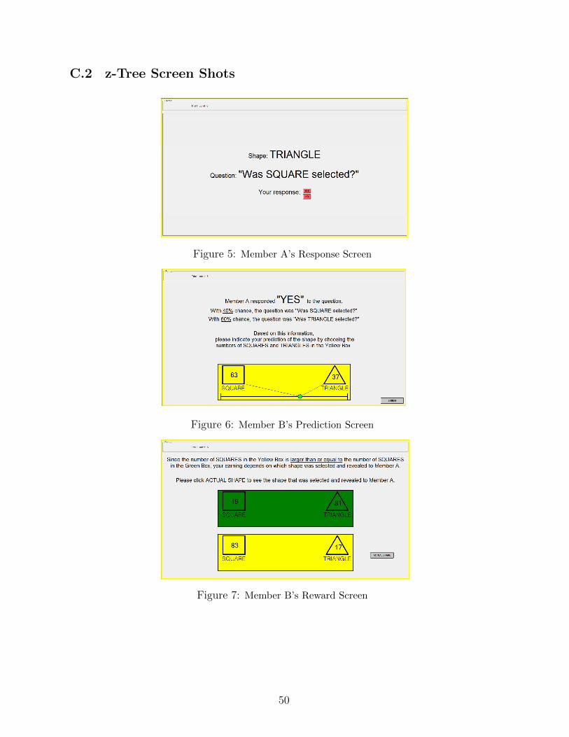
C.2 z-Tree Screen Shots

Training round: The first screen of the sender subject.Figure 5: Member A’s Response Screen

Figure 6: Member B’s Prediction Screen

The number of SQUARES in the GREEN BOX is revealed. In this example, the YELLOW BOX has more SQUARES than the GREEN BOX. So, the reward will be determined by the actual shape Pressing the button “ACTUAL SHAPE” showsdetermined by the actual shape. Pressing the button  ACTUAL SHAPE  shows the selected shape in the next screen.

Figure 7: Member B’s Reward Screen

50