elisa helena fernandes.pdf
TRANSCRIPT
Modelling the Hydrodynamics of the Patos Lagoon, Brazil
by
Elisa Helena Fernandes
A thesis submitted to the University of Plymouth in partial fulfilment for the degree of
Doctor of Philosophy
Institute of Marine Studies Faculty of Science
October 2001
90 0497856 7
LIBRARY STORE
Lagoa dos Patos
no fundo da lagoa
Dorme uma saudade boa
Longe desse c6u sereno
O coragao pequeno
E vazio ficou
Sei que a vida igou as velas
Mas em noites belas
Sou navegador
LA no fundo da lembranga
Dorme urn resto de esperanga
De voltara vida a tea
A beira da lagoa
S6 molhando o p4
Seja em Tapes, Sao Lourengo
Barra do Ribeiro ou Arambar6
Lagoa dos Patos
Dos sonhos, dos barcos
Mar de dgua doce e paixao
Ah! Essa cangao singela
Eu fiz s6 pra ela
Nao me leve a mal
Eta que 4 fifha da lua
Que ilumina as mas
LA do Laranjal.
Kledirnamil& Fogaga (1981).
Modelling the Hydrodynamics of the Patos Lagoon, Brazil Elisa Helena Ledo Femandes
Abstract
The Palos Lagoon, the largest choked coastal lagoon in the world, is a typical centre of population,
commerce, industry and recreation, and consequently it is also a site for disposal of industrial,
agricultural and municipal wastes. Important questions concerning beneficial uses of and potential
changes to the lagoon and its estuary are left unanswered without a good understanding of
hydrodynamic processes. The current study involves the choice, calibration and application of a
numerical model which can be used in future hydrodynamic. sediment transport and water quality
studies in the area.
The two- and three-dimensional modes of the TELEMAC System were chosen to study the
hydrodynamics of the Patos Lagoon. In order to calibrate the TELEMAC-2D model for the lagoon,
measurements of salinity, current speed and direction, water elevation and wind speed and
direction were carried out simultaneously at three stations in the estuarine area during three days.
The model validation was carried out against an independent data set from the 1998 El Nino event.
Several two-dimensional simulations were carried out to investigate the main processes controlling
the Patos Lagoon hydrodynamics. The model was forced with prescribed river inflow at the top of
the lagoon, wind stress at the siuface and water elevation at the ocean boundary. The barotropic
pressure gradients established between the lagoon and the coastal area as a result of local and
remote wind combined with the freshwater discharge, proved to be the main forces controlling the
lagoon subtidal circulation, as well as the exchanges between the lagoon and the coast. The local
wind dominates the lagoon circulation through the set-up/set-down mechanism of oscillation,
whereas the non-local wind drives the circulation in the lower estuary. The entrance channel acts as
a filter and strongly reduces tidal and subtidal oscillations generated offshore.
Three-dimensional simulations proved to be essential. Studies of the processes involved in the
estuarine transverse circulation showed that the wind drives the lateral flow in the shallow areas,
whereas in the channel it depends on lateral pressure gradients and channel curvature and
geometry. Insights on the estuarine baroclinic circulation indicate the barotropic forces as the main
mechanism controlling salt water penetration and salinity structure in the estuary.
This study produced valuable information into the forces controlling the circulation of the Patos
Lagoon and its estuary. Important issues regarding the capabilities of the TELEMAC System two-
and three-dimensional modules were explored, producing a valuable tool for further hydrodynamic
and sediment transport numerical modelling experiments.
Contents
Chapter 1: Introduction
1.1. W h y study the Patos Lagoon? 1 1.2. A i m and objectives 4 L 3 . Outline o f the thesis 4
Chapter 2: The Patos Lagoon
2.1. General aspects about coastal lagoons 6 2.1.1. Geomorphology 7 2.1.2. Circulation 10 2.2. About the Patos Lagoon 12 2.2.1. General aspects 12 2.2.2. Settlement and history 14 2.2.3. Regional climate 15 2.2.4. River f l o w 17 2.2.5. Tidal forcing and wind effect 19
Chapter 3: Description of the Fieldwork 27
3.1. Introduction 27 3.2. Fieldwork strategy 27 3.3. Instrumentation 29 3.3.1. Current measurements 29 3.3.2. Salinity and temperature measurements 31 3.3.3. Wind measurements 31 3.3.4 Water level measurements 32 3.3.5. Suspended matter and bottom sediment sampling 32
3.4. Measurements in the channel 33 3.4.1. Velocity components 33 3.4.2. Wind 39 3.4.3. Water level 40 3.4.4. Salinity 41 3.4.5. Suspended matter 44 3.5. Measurements in the shallow area 49 3.5.1. Velocity components, wind and water depth 49 3.5.2. Salinity and suspended matter 52
Chapter 4: Description of the Model 55
4.1 . Introduction 55 4.2. The T E L E M A C System 56 4.3. T E L E M A C - 2 D model 57 4.3.1. Notation and basic geometry 57 4.3.2. The Navier-Stokes equations 59 4.3.3. Hypothesis and approximations 60 4.3.4. Source terms of the momentum equation 61 4.3.5. Boundary conditions 63 4.3.6. Turbulence modelling 64 4.3.7. Tidal flats 65 4.3.8. Numerical methods 66 4.4. T E L E M A C - 3 D model 67
Chapter 5: Calibration and Validation of the Model 73
5.1. Introduction 73 5.2. Sensitivity tests 73 5.3. Mesh resolution tests 79 5.4. Calibration o f the mode! 83 5.5. Validation of the model 95
Chapter 6; The Patos Lagoon Two-dimensional Circulation 99
6.1. Introduction 99 6.2. W i n d effect 99 6.3. The Patos Lagoon response time to wind forcing 106 6.4. Effect o f the Freshwater discharge 112 6.5. The Patos Lagoon tidal and subtidal circulation (January 1992) 119 6,5,1. Tidal and subtidal attenuation 128 6.6. The Patos Lagoon hydrodynamics between 27-29/10/1998 133 6.7. The Patos Lagoon hydrodynamics during an E! Nino event (1998) 135
Chapter 7: The Patos Lagoon Three-dimensional Circulation 152
7.1. Introduction 152 7.2. Longitudinal and transverse flow in the estuary 152 7.3. Model l ing salinity distribution in the estuary 160 7.4. Salinity propagation 165 7.5. Estuarine mixing 170
111

Chapter 8: Discussions, Conclusions and Future Work 175
8.1. W h y T E L E M A C ? 175 8.2. T E L E M A C - 2 D vs. T E L E M A C - 3 D 176 8.3. Conclusions 179 8.4. Future work 182
References 184
IV
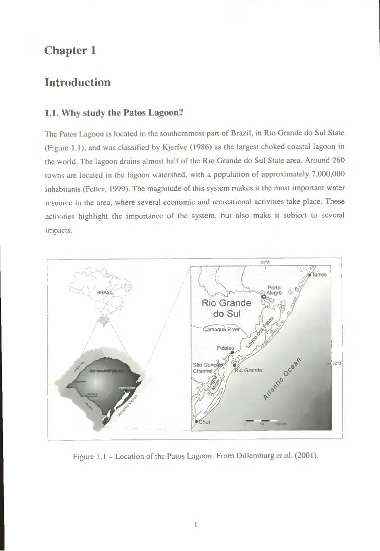
List of Figures Figure 1.1. Location o f the Patos Lagoon. From Dil lemburg et al. (2001). 1
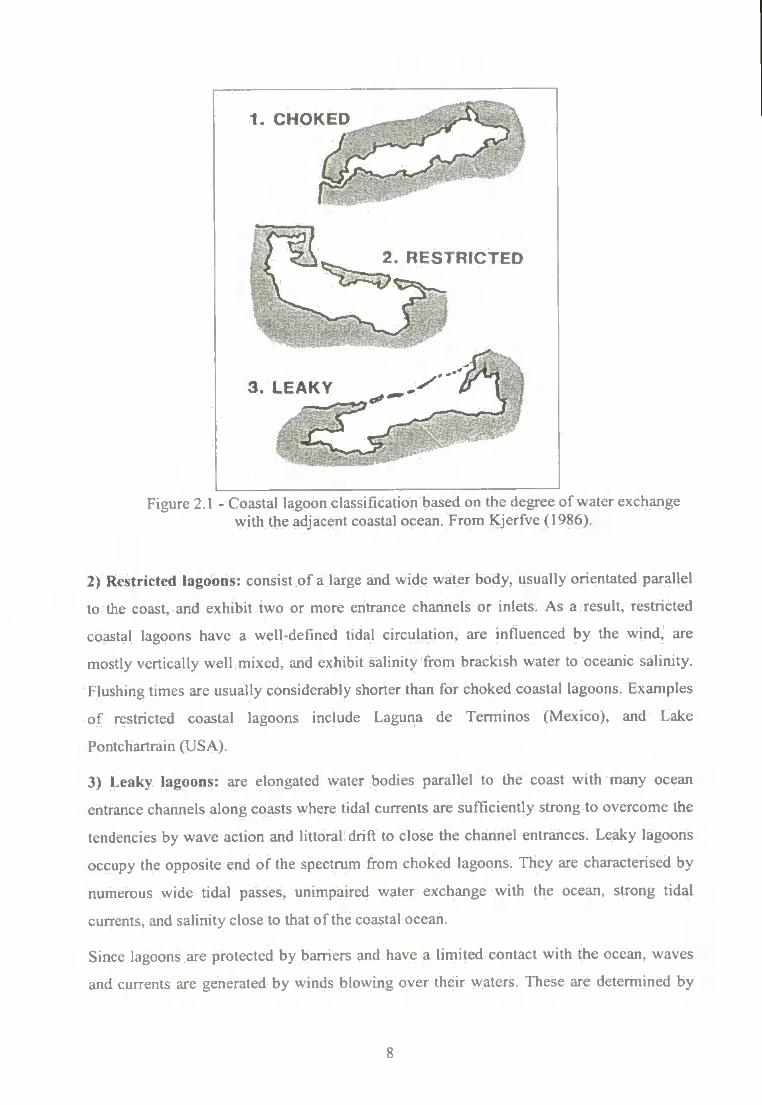
Figure 2 .1 . Coastal lagoon classification based on the degree o f water exchange 8 with the adjacent coastal ocean. From Kje r fve (1986).
Figure 2.2. Theoretical model of septation stages o f coastal lagoons due to wind 9 effects. From Isla(1995).
Figure 2.3. The Patos Lagoon System. 13
Figure 2.4. Rio Grande channel bathymetric charts f r o m 1885 ( A ) and 1988 (B) . 15 From Fetter (1999).
Figure 2.5. Prediction of a regional model (CPTEC/INPE) for 8/7/99, showing the 16 two anticyclones.
Figure 2.6. Freshwater contribution f r o m Jacui-Taquan and Camaqua river 18 systems during one year of measurements (1988).
Figure 2.7. Energy spectra of the water level time series recorded at Rio Grande, 21 Arambar6 and Itapoa (12/1987-01/1998). From Mol le r et al (1996).
Figure 2.8. The channel as a filter. From Mol ler et al. (1996). 22
Figure 2.9. Calculated water levels f r om the model experiment carried out without 23 wind forcing. From Mol ler (1996).
Figure 2.10. Calculated water levels f r o m the model experiment including the local 24 wind. From Mol ler (1996).
Figure 2.11. Schematic representation o f the level oscillation in the lagoon under 25 NE ( A ) and SW (B) wind. From Fetter (1999).
Figure 3.1. The Patos Lagoon estuary and stations. 28
Figure 3.2. Velocity components at Feitoria, Marambaia and Barra do Rio Grande 34 stations on the 27/10/1998.
Figure 3.3. Velocity components at Feitoria, Marambaia and Praticagem stations 35 on the 28/10/1998.
Figure 3.4. Velocity components at Feitoria and Marambaia stations on the 36 29/10/1998.
Figure 3.5. Overnight velocities at the shallow area around Feitoria. ( A ) 38 26/10/1998, (B) 27/10/1998, and (C) 28/10/1998.
Figure 3.6. Wind speed and direction at Feiioria ( A ) and Marambaia (B) station. 39
Figure 3.7. Wind velocity components at Praticagem station between 20- 40 29/10/1998. WX is positive to the East and WY is positive to the North.
Figure 3.8. Water elevation at Praticagem station between 20-29/10/1998. 40
Figure 3.9. Salinity profiles al Pralicagem ( A ) and Marambaia (B) on the 42 27/10/1998.
Figure 3.10. Salinity profiles at Praticagem ( A ) and Marambaia (B) on the 43 28/10/1998.
Figure 3.11. Salinity proHle at Marambaia on the 29/10/1998. 44
Figure 3.12. Suspended matter profiles at Feitoria ( A ) , Marambaia (B) and Barra 46 do Rio Grande (C) on the 27/10/1998.
Figure 3.13. Suspended matter profiles at Feitoria ( A ) , Marambaia ( B ) and 47 Praticagem (C) on the 28/10/1998.
Figure 3.14. Suspended matter profiles at Feitoria ( A ) , Marambaia ( B ) on the 48 29/10/1998.
Figure 3.15. Velocity components ( A ) , w ind speed and direction (B) and water 50 depth (C) at Porto Rei station on the 05/11/1998. Measurements started at 08:45 am.
Figure 3.16. Velocity components ( A ) , w ind speed and direction (B) and water 51 depth (C) at Porto Rei station on the 06/11/1998. Measurements started at 09:00 am.
Figure 3.17. Salinity and suspended matter concentration at Porto Rei station. 52 05/11/1998 and (B) 06/11/1998.
Figure 3.18. Relation between suspended matter and cross-channel velocity at 53 Porto Rei station. (A) 05/11/98 and (B) 06/11/98.
Figure 4 .1 . The T E L E M A C System. 58
Figure 4.2. Defini t ion of bottom topography and free surface. 58
Figure 4.3. Three-dimensional mesh obtained by superimposition o f two- 70 dimensional meshes.
Figure 5.1. Water elevation measured at Praticagem by the Rio Grande Pilots 74 between 11-13/01/1992.
Figure 5.2. Finite element mesh wi th 1175 nodes and 2048 triangles. 74
Figure 5.3. Longitudinal velocity at Praticagem (node 80) calculated using the ( A ) 76 Manning, (B) Chezy, and (C) Nikuradse laws of bottom fr ic t ion .
Figure 5.4. Patos Lagoon circulation pattern when using the Chezy law o f bottom 77 fr ict ion (A) C=37, (B) C=65, (C) C=100.
Figure 5.5. Eddy viscosity sensitivity tests ( A ) Ve=0.01, (B) v e =0 .1 , (C) v e = 1 , (D) V e =10, (E) V e =100, and (F) v e =1000.
Figure 5.6. Estuarine space discretization at ( A ) low, (B) medium and (C) high 80 resolution used for the mesh resolution tests.
Figure 5.7. Calculated and observed longitudinal velocity at Praticagem for three 81 different meshes: ( A ) low (B) medium, and (C) high resolution.
Figure 5.8. M E S H l space discretization for the lagoon ( A ) and low estuary (B) . 82
Figure 5.9. Calculated and observed longitudinal velocity at Praticagem using 82 M E S H l ,
Figure 5.10. Water elevation and wind data used to force the model between 20- 85 26/10/1998 (A ,B) and 27-29/10/1998 (C,D). WX is positive to the East and WY is positive to the North.
VI
Figure 5.11. Atmospheric pressure used to force the model between 27-29/10/1998. 86 ( A ) at the top o f the lagoon, (B) at the mouth o f the estuary.
Figure 5.12. Results f r om the calibration tests fo r the first day o f simulation at 88 Feitoria ( A ) and Marambaia (B) when using the Manning law of bottom fr ic t ion .
Figure 5.13. Results f r o m the calibration tests fo r the second day of simulation at 89 Praticagem when using the ( A ) Manning, (B) Chezy and (C) Nikuradse laws of bottom fr ic t ion.
Figure 5.14. Calculated and observed lateral velocities around Feitoria. ( A ) 91 26/10/98, (B) 27/10/98, (C) 28/10/98.
Figure 5.15. Bottom fr ict ion distribution for testing the spatially varying fr ic t ion. 92
Figure 5.16. Comparison o f (A) longitudinal velocities at Rio Grande and (B) 94 inf low/out f low of water produced wi th constant and varying fr ic t ion.
Figure 5.17. Comparison between measurements and predicted longitudinal 95 velocities when using constant f r ic t ion and f r ic t ion varying according to bed sediment at Praticagem.
Figure 5.18. Water elevation ( A ) and wind velocity (B) time series used for the 97 model validation simulation.
Figure 5.19. Comparison between measurements and modelling results at SJN, 98
Figure 6.1. Finite element mesh wi th 2631 triangles ( L A G O A 1 4 ) . 101
Figure 6.2. Velocity vectors for the N E wind forcing after ( A ) 6h, (B) 24h, and 102 (C) 72h o f simulation.
Figure 6.3. Velocity vectors for the SW wind forcing after ( A ) 6h, (B) 24h, and 104 (C) 72h o f simulation.
Figure 6.4. The wind effect on the water elevation after 6 hours of simulation 105 when prescribing (A) NE and (B) SW winds.
Figure 6.5. Water elevation data f rom Praticagem (11-13/01/1992) used as 106 dynamic ocean boundary condition.
Figure 6.6. Comparison o f predictions obtained wi th a constant and dynamic 107 ocean boundary condition at (A) Arambar^, (B) Rio Grande, and (C) Praticagem.
Figure 6.7. Initial conditions (NE wind) and the lagoon response time to different 109 wind directions at Itapoa (A , B) , Feitoria (C, D ) , and Marambaia (E, F).
Figure 6.8. The lagoon response time to different wind directions at the Itapoa HO ( A ) , Feitoria (B) , and Marambaia (C) in the first 24 hours o f simulation.
Figure 6.9. Initial conditions (SW wind) and the lagoon response time to different 111 wind directions at Itapoa (A , B) , Feitoria (C, D ) , and Marambaia (E, F).
Figure 6.10. The Patos Lagoon kinetic energy when forced with SW wind. From 112 Fetter (1999).
V I I
Figure 6.11. Time series o f water elevation measured at Praticagem in January 113 1992.
Figure 6.12. Predicted time series of the water elevation (m) at Itapoa ( A ) and 114 Feitoria (B) for different freshwater discharges.
Figure 6.13. Water elevation (m) through out the lagoon after ( A ) 147, (B) 459, and 116 (C) 672 hours o f simulation when prescribing 1000 s *.
Figure 6.14. Water elevation (m) through out the lagoon after ( A ) 147, (B) 459, and 116 (C) 672 hours o f simulation when prescribing 5000 m^ s"'.
Figure 6.15. Velocity vectors after 19 days o f simulation when prescribing a 117 discharge o f ( A ) 1000 m^ s * and (B) 5000 m^ s *.
Figure 6.16. Zoom of the velocity vectors after 19 days of simulation when 118 prescribing a discharge of ( A ) 1000 m"* s ' and (B) 5000 m"* s *.
Figure 6.17. Energy spectrum of the time series o f water elevation - January 1992. 120
Figure 6.18. Time series of water elevation. (A) unfil lered data, (B) high frequency 121 data, and (C) low frequency data.
Figure 6.19. Locations used to study the tidal and subtidal effect. 122
Figure 6.20. Predicted water elevation at ( A ) Praticagem, (B) Canal, (C) Rio 123 Grande, and (D) Feitoria under the tidal influence.
Figure 6.21. Predicted water elevation at (A) Praticagem, (B) Canal, (C) Rio 125 Grande, and (D) Feitoria under the subtidal influence.
Figure 6.22. Predicted velocity vectors through out the lagoon after 15 days o f 126 simulation. (A) tidal forcing, (B) subtidal forcing.
Figure 6.23. Predicted velocity vectors through out the estuary after 15 days of 127 simulation. ( A ) tidal forcing, (B) subtidal forcing.
Figure 6.24. Power spectrum of the tidal signal used to force the model. 129
Figure 6.25. Cross-spectrum results when applying the tidal forcing. Co-spectrum, 130 coherence and phase spectrums at ( A ) Praticagem, (B) Canal, (C) Rio Grande, (D) Marambaia and (E) Feitoria.
Figure 6.26. Power spectrum of the subtidal signal used to force the model. 131
Figure 6.27. Cross-spectrum results when applying the subtidal forcing. Co- 132 spectrum, coherence and phase spectrums at ( A ) Praticagem, (B) Canal, (C) Rio Grande, (D) Marambaia and (E) Feitoria.
Figure 6.28. Predicted estuarine longitudinal and transverse velocities and water 136 elevation time series (27/10/1998). ( A ) Feitoria, (B) Marambaia, (C) Praticagem.
Figure 6.29. Predicted estuarine longitudinal and transverse velocities and water 137 elevation time series (28/10/1998). ( A ) Feitoria. (B) Marambaia, (C) Pralicagem.
Figure 6.30. Predicted estuarine longitudinal and transverse velocities and water 138 elevation time series (29/10/1998). ( A ) Feitoria. (B) Marambaia, (C) Praticagem.
vni
Figure 6.31. Predicted circulation during the first day o f simulation at the lagoon 139 (A) and estuary (B) .
Figure 6.32. Predicted circulation during the second day o f simulation at the lagoon 140 (A) and estuary (B) .
Figure 6,33. Predicted circulation during the third day o f simulation at the lagoon 141 ( A ) and estuary (B) .
Figure 6.34. Water elevation ( A ) and wind velocity (B) used fo r the El Ni f io 143 simulations. WX is positive to the East and WY is positive to the North.
Figure 6.35. Surface elevation (single line) and longitudinal velocity (marked line) 144 through out time for ( A ) Itapoa, (B) Feitoria. and (C) Praticagem.
Figure 6.36. ( A ) Velocity vectors (m s"*) and (B) water elevation (m) along the 146 lagoon after 1 day of simulation when prescribing a river in f low 8000
m s
Figure 6.37. (A) Velocity vectors (m s *) and (B) water elevation (m) along the 147 lagoon after 10 days o f simulation when prescribing a river inf low 8000 m^ s ' .
Figure 6.38. Comparison between the variation of the Patos Lagoon volume 148 through time against ( A ) the water elevation and (B) w i n d velocity data used to force the model during the El Nino simulations.
Figure 6.39. In f low and outf low f r o m the lagoon to the coastal area during the 18 150 day-simulation for the three freshwater discharges tested. Positive indicates landwards flow, and negative indicates seawards flow.
Figure 6.40. R A D A R S A T image f r o m the Canadian Remote Sensing Centre 151 processed by the Physical Oceanography Laboratory at the University of Rio Grande (FURG). A p r i l 1998.
Figure 7 .1 . Vertical cross sections throughout the estuary indicating the distance 153 f rom the mouth.
Figure 7.2. Vertical sections o f along-estuary (contours) and cross-estuary 156 (vectors) flow at Feitoria after 5h ( A ) , lOh (B) and 70h (C) of simulation when prescribing N E wind. Free surface elevation plots are at the top o f each cross section, respectively.
Figure 7.3. Vertical sections of along-estuary (contours) and cross-estuary 157 (vectors) flow at SJN after 5h ( A ) , lOh (B) , 15h (C) and 70h (D) of simulation when prescribing N E wind. Free surface elevation plots are at the top of each cross section, respectively.
Figure 7.4. Vertical sections o f along-estuary (contours) and cross-estuary 158 (vectors) flow at Feitoria after 5h ( A ) , lOh (B) and 70h (C) of simulation when prescribing SW wind. Free surface elevation plots are at the top o f each cross section, respectively.
Figure 7.5. Vertical sections of along-estuary (contours) and cross-estuary 159 (vectors) flow at SJN after 5h ( A ) , lOh (B) , 15h (C), and 70h (D) of simulation when prescribing SW wind. Free surface elevation plots are at the top o f each cross section, respectively.
IX
Figure 7.6. Water elevation ( A ) and wind ( B ) data used to force the model 162 between 27-29/10/1998. WX is positive to the East and WY is positive to the North.
Figure 7.7. Longitudinal velocity during the first 36 hours of simulation at the 163 vertical cross-section C. Wid th = 3.7 km.
Figure 7.8. Salinity during the first 36 hours o f simulation at the vertical cross- 164 section C. Wid th = 3.7 km.
Figure 7.9. Longitudinal velocity during the last 36 hours o f simulation at the 166 vertical cross-section D . Wid th = 4.4 km.
Figure 7.10. Salinity during the last 36 hours o f simulation at the vertical cross- 167 section D . Width = 4.4 km.
Figure 7.11. Velocity vectors and salinity penetration at the surface, middle depth 168 and bottom after 16 hours of simulation.
Figure 7.12. Velocity vectors and salinity penetration at the surface, middle depth 169 and bottom after 64 hours o f simulation.
Figure 7.13. Richardson number at vertical cross-section C. Wid th = 3,7 k m . 173
Figure 7.14. Richardson number at vertical cross-section D . Wid th = 4.4 k m . 174
Figure 8.1. Longitudinal velocity profiles at Feitoria (28/10/1998). 177
Figure 8.2. Longitudinal velocity profiles at Praticagem (28/10/1998). 178
Figure 8,3. Comparison between measured and predicted (/n=0,025) depth- 179 averaged longitudinal velocity at Praticagem (28/10/1998).
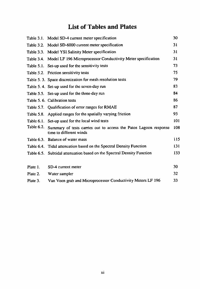
List of Tables and Plates Table 3.1. Model SD-4 current meter specification 30
Table 3.2. Model SD-6000 current meter specification 31
Table 3.3. Model Y S I Salinity Meter specification 31
Table 3.4. Model L F 196 Microprocessor Conductivity Meter specification 31
Table 5.1. Set-up used for the sensitivity tests 73
Table 5.2. Friction sensitivity tests 75
Table 5. 3. Space discretization for mesh resolution tests 79
Table 5. 4. Set-up used for the seven-day run 83
Table 5.5. Set-up used for the three-day run 84
Table 5. 6. Calibration tests 86
Table 5.7. Qualification of error ranges for RMAE 87
Table 5.8. Applied ranges for the spatially varying friction 93
Table 6.1. Set-up used for the local wind tests 101 Table 6.2. Sunmiary of tests carries out to access the Patos Lagoon response 108
time to different winds
Table 6.3. Balance of water mass 115
Table 6.4. Tidal attenuation based on the Spectral Density Function 131
Table 6.5. Subtidal attenuation based on the Spectral Density Function 133
Plate 1. SD-4 current meter 30
Plate 2. Water sampler 32
Plate 3. Van Veen grab and Microprocessor Conductivity Meters L F 196 33
XI
Acknowledgements
V 1 would tike to express my gratitude for the excellent guidance and supervision of Professor
Keith Dyer, my supervisor. Thanks so much so being there all the time. You wi l l always have a
place in my heart.
V Many thanks to Mr. John Baugh for being on the other end of the line the whole time, giving me
unconditional support and encouragement, and to HR Wallingford for providing the TELEMAC
model and support. I am also grateful to Mr. Steve Gibson, Mr. Tony Moore and Mrs. Sandra
Chenery, from PML. for their support with the workstation management.
¥ I am indebted to several people who made my fieldwork possible in Brazil, especially Dr. Luis
Felipe Niencheski, Ms. Lucia Bohmer. and Mr. Vanderien Miranda for their support and for the
infrastructure of the Laboratdrio de Hidroqufmica (FURG). Many thanks to all the fieldwork
participants and crew members, and to the Rio Grande Pilots - Praticagem da Barra for kindly
providing infrastructure and data for this research. 1 can't forget a special thank you to my good
friend Ari ... I f you ever need to relax again, we can certainly arrange another fieldwork!
V Thanks also to Dr. Osmar Moller for providing equipment for the fieldwork and data for the El
Nino simulations, to Dr. Carlos Hartmann for analysing the sediment samples and providing data
from January 1992, and to Dr. Ken George for comments and discussions throughout this research.
V A formal thank you goes to the Conselho Nacional de Desenvolvimento Cienttfico e Tecnoldgico
(CNPq) for sponsoring this research at the University of Plymouth.
V A big thank you goes to all my friends. The ones I had to stay apart, and the ones I had the
pleasure to share the last four years of my life. Your words of support, advise and encouragement
were essential, and all the happy moments we had together are unforgettable. I would like to
mention: Giovanni & Sandrine. Lu & Nico. Ronald & Tali. Sergio & Patricia. Cova & Pablo,
Cecflia & Ismael. Claudia & Eduardo, James & Linda, Leonardo & Fabiana, Marquinhos & Cama,
Lu & Marisa. Eilis & Sennan. Susana & Antonio. Stuart & Harriet, Herman {in memorium),
Xavier, Susana Die, Kelmo, Eleine, Cyril, Brad, Mark P., Malcolm, Christophe, Jon. Dave, and
other members o f the famous "Coffee CIub'\
¥ To my parents, Valcir & Irene: Obrigado por estarem sempre ao meu lado. Sent o apoio e o
amor de voces nada disto seria possivel.
V And Gilberto... A l l my love goes to you. Thank you so much for putting up with all this and for
being there... always.
xn
Author's Declaration
A t no time during the registration fo r the degree of Doctor o f Philosophy has the author
been registered for any other University award.
Publications
Femandes. E.H.L. ; Dyer, K.R. & Moller , O.O., 2001. On the hydrodynamics o f the
worid's largest choked coastal lagoon: Palos Lagoon, Brazil . Estuaries, in press.
Femandes, E.H.L. ; Dyer. K.R. & Niencheski, L .F .H. , 2001. Calibration and validation of
the T E L E M A C - 2 D model to the Patos Lagoon (Brazil) . Journal of Coastal Research
Special Issue - International Coastal Symposium 2000, in press,
Femandes, E.H.L. ; Dyer, K.R.; Moller , O.O. & Niencheski, L .F .H . The Patos Lagoon
hydrodynamics during an El Nino event (1998). Continental Shelf Research Special Issue
- Physics of Estuaries and Coastal Seas 2000, in press.
Presentations and Conferences Attended
• T E L E M A C - 2 D Workshop. HR Wal l ingford , U K , 24-25 March 1998
• U K Oceanography 98, University o f Southampton, U K . 7-11 September 1998.
• T E L E M A C - 3 D Workshop, HR Wal l ingford . U K , 14 A p r i l 1999.
• T E L E M A C USERS C L U B M E E T I N G , EDF - Paris, 18-19 November 1999.
• International Coastal Symposium 2000, Rotorua, New 2^aland. 24-28 A p r i l 2000. Oral
presentation
• 10* International Biennial Conference on Physics o f Estuaries and Coastal Seas,
Norfolk , Virginia, USA, 7-11 October 2000. Poster presentation.
• Seminar at the Institute of Marine Studies, University o f Plymouth, March 1999.
• Seminar at Plymouth Marine Laboratory - PERC, Plymouth, M a y 2000,
• Seminar at Proudman Oceanographic Laboratory, Liverpool , October 2000,
Signature kdU^xCJ fuxxXXuxk
x n i
Modelling the Hydrodynamics of the Patos Lagoon, Brazil
by
Elisa Helena Femandes
X I V
Chapter 1
Introduction
1.1. Why study the Patos Lagoon?
The Patos Lagoon is located in the southernmost part of Brazil, in Rio Grande do Sul State
(Figure 1.1), and was classified by Kjerfve (1986) as the largest choked coastal lagoon in
the world. The lagoon drains almost half of the Rio Grande do Sul State area. Around 260
towns are located in the lagoon watershed, with a population of approximately 7,000,000
inhabitants (Fetter, 1999). The magnitude of this system makes it the most important water
resource in the area, where several economic and recreational activities take place. These
activities highlight the importance of the system, but also make it subject to several
impacts.
BRASIL
Grande
Channei
32^
Figure 1.1 - Location of the Fatos Lagoon. From Dillemburg et al. (2001).
Navigational activities are very important in the lagoon. Rio Grande Harbour, located at
Rio Grande City, has intense port activity and is one of the main harbours in Brazil,
comprising the biggest bulk complex of Latin America*. Artificial channels maintained by
dredging make navigation possible throughout the lagoon and connect Rio Grande
Harbour to the second main harbour in the state, located at Porto Alegre City. These
harbours and their access channels receive high quantities of suspended matter from the
riverine system located in the north of the lagoon, promoting their sillation and making
frequent dredging essential.
Fishing also has an important socio-economical role in the communities located on the
margins of the lagoon. As approximately 80% of the estuarine area is less than 2 m deep,
the lagoon is a nursery ground for important commercial fish and shrimp species,
sustaining a fishery production of 182 kg ha * year"' (Castello. 1985). Some of these
species are dependent on salt water penetration making the monitoring and prediction of
salty water circulation an important issue in the area
Agriculture is another important economic activity in the area. The main crops in the north
of Rio Grande do Sul State are com, soy, wheat, tobacco and beans, whereas rice crops are
dominant in the south. Several paddy fields are concentrated on the western margin of the
Patos Lagoon. They are highly sensitive to salt water and highlight once again the
importance of monitoring and predicting salt water circulation.
A combination of agricultural wastes and several others industrial and human
contributions are carried from the drainage basin into the lagoon by the freshwater
discharge. The riverine discharge is usually the dominant source of material input into
coastal lagoons, transporting dissolved and suspended particulate materials and bedload
from the drainage basin (Kjerfve & Magill, 1989). When such contributions occur in
moderation, the input of nutrients and sediment enhance lagoon productivity, but when in
excess, such inputs can cause eutrophication.
The river discharge coming from the Jacui-Taquari riverine system carries a variety of
agricultural wastes combined with wastes from the petro-chemical industrial park located
at Porto Alegre City (1,360,000 inhabitants^) and the untreated domestic sewage from the
area. The Camaqua River is marked by serious erosion problems and carries into the
' Zero Hora, 18'*' March 1997, pp.39. Special Report: Porto de Rio Grande apresenta problemas na drea ambienlal. ^ Instituto Brasileiro de Geografia e Estatistica (IBGE), Census 2000, http://wwwl.ibge.gov.br/ibge.
central lagoon high concentrations of suspended matter, associated with more agricultural
wastes.
The estuarine area extends 60 km inland from the mouth and receives a variety of
contributions. The Sao Gon^alo Channel carries agricultural wastes from the Mirim
Lagoon watershed and the untreated sewage from Pelotas City (323,000 inhabitants^). The
area around Rio Grande City (186,500 inhabitants^) receives industrial effluents from the
fertiliser and oil refinery companies and the untreated sewage from the city. The discharge
of all these organic and inorganic contaminants (e.g. nutrients, heavy metals, pesticides)
into the lagoon causes severe impacts, which could be better understood through
modelling predictions of the dispersion of contaminants and water quality.
Thus, it is clear that several issues concerning dredging of access channels, disposal of
dredged material, dispersion of organic and inorganic contaminants, interaction processes
between the seabed and the water column and water quality studies are extremely
important for the area. The first step to carry out these studies is to have a good
understanding of the hydrodynamics of the lagoon and esluarine areas, and numerical
modelling techniques are valuable tools towards this understanding. The combination of
the hydrodynamic model with sediment transport and water quality models is the next step
forward.
Data and hydrographic information have been collected in the area since the last century,
helping to produce the first hydrodynamic studies (Bicallho, 1883; Von Ihering, 1885;
Malaval, 1915; 1922; Gaffree, 1927; Motta, 1969). Although recently several others used
measurements and modelling techniques to improve this understanding (Moller, 1996;
Moller et a/., 1996; 2001; Castelao, 1999; Fetter, 1999), there are still many aspects of the
Patos Lagoon hydrodynamics to be revealed. On the other hand, until now none of the
modelling studies about the hydrodynamics of the lagoon offered the possibility of easily
incorporating in the hydrodynamics further modules to predict important issues such as
the transport of cohesive sediment and water quality.
^ Insiituto Brasileiro de Geografia e EstaU'stica (IBGE). Census 2000, http://wwwl.ibge.gov.br/ibge.
1.2* Aim and Objectives
The approach adopted for this research involves the choice, calibration, and application of
a numerical model capable of accurately dealing with the complexity of the Patos Lagoon
system in order to have an important tool for future hydrodynamic, sediment transport and
water quality predictions.
The main objectives of this research were:
• To carry out field measurements in the lagoon to provide the boundary conditions for
the model,
• To calibrate and validate the numerical model with two independent data sets,
• To study the Patos Lagoon response to the main forcing factors using a two-
dimensional numerical model,
• To explore the Patos Lagoon two- and three-dimensional hydrodynamics during
specific events,
• To study the barotropic and baroclinic effects on the three-dimensional circulation,
• To assess the necessity of using two- or three-dimensional numerical models in the
area.
1.3. Outline of the Thesis
Chapter 2 presents a literature review of the main aspects about coastal lagoons discussed
in this thesis, followed by a detailed description of the geographical, hydrological and
dynamical characteristics of the Palos Lagoon. The fieldwork carried out in the Patos
Lagoon estuary for data to be used as boundary conditions in the model is described in
Chapter 3, giving details about the instrumentation, strategy and results obtained. Chapter
4 initially presents an overview of numerical modelling in general and the finite element
technique in particular. The structure of the TELEMAC System (EDF, Paris) is then
presented, followed by a description of the main assumptions, equations and numerical
methods used in the two-dimensional (TELEMAC-2D) and three-dimensional
(TELEMAC-3D) modules.
Chapter 5 describes in detail several sensitivity and calibration tests carried out with
TELEMAC-2D. Sensitivity tests were initially carried out to determine the model
sensitivity to variations in the friction and horizontal eddy viscosity parameters, the
Coriolis force and the space discretization. Calibration tests were carried out by semi
quantitative) y comparing time series of longitudinal velocity produced by the model with
field data, defining the parameters that give the best fit between the two. The last step was
to validate the model with an independent data set.
Chapter 6 presents several numerical experiments with the TELEMAC-2D model to
investigate the main factors controlling the Patos Lagoon hydrodynamics. The local and
non-local wind effects are initially considered, followed by the effect of the freshwater
discharge and the tidal and subtidal circulation in January 1992. The model was then used
to predict the hydrodynamics of the lagoon during two specific periods of interest when
field data is available. The first concentrates on the period when fieldwork was carried out
in the lagoon, and the second during an El Nino event.
Some three-dimensional aspects of the Patos Lagoon hydrodynamics are presented in
Chapter 7. Initially, results from two vertical cross-sections in the estuary are presented to
illustrate the effect of barotropic forces on the longitudinal flow, and the possible
mechanisms involved in the estuarine transverse circulation during the two predominant
wind situations. Secondly, the model starts to take into account the baroclinic forces, and a
salinity penetration event is explained based on the observed barotropic forces. Finally, the
three-dimensional numerical modelling of the salinity distribution in the estuary is used to
estimate the intensity of mixing occurring at different times and at different positions in
the estuary based on the predicted Richardson number.
Chapter 8 presents discussions of the requirement for two- or three-dimensional modelling
in studying the Patos Lagoon hydrodynamics, and the main conclusions of this research.
Recommendations for future work are also discussed.
Chapter 2
The Patos Lagoon
2.1. General aspects about coastal lagoons
Coastal lagoons border more than 13%, or 32,000 km, o f the world's continental coasts
(Barnes, 1980; Knoppers & Kjerfve, 1999). They are found in a variety of environments,
ranging from arctic to equatorial, and from arid to humid (Lasserre, 1979; Guilcher, 1981),
and on a variety of scales, from over 10,000 km^ (Patos Lagoon, Brazil) down to less than
a hectare (Bird, 1994). They are most common along microtidal, high wave energy coasts
(Kjerfve & Magill, 1989). where the coastal plain has been subjected to submergence
during Holocene sea-level rise, and alternatively flooded and exposed by sea-level
fluctuations during the late-Quaternary period (Nichols & Allen, 1981). The age of
present-day lagoons is 5000-6000 years, but varies according to the local amplitudes of
marine transgression and regression phases, tidal range, shoreface dynamics, availability of
coastal sandy sediments, fluvial transport, and climate (Bird, 1994; Knoppers & Kjerfve,
1999)
According to Kjerfve (1994), coastal lagoons experience forcing from river input, wind
stress, tides, precipitation - evaporation balance, and surface heat balance, and respond
differently to these forcing functions. Water and salt balances, lagoon water quality, and
eutrophication depend critically on lagoon circulation, salt and material dispersion, water
exchange with the ocean, and turn-over, residence, or flushing times.
In general, coastal lagoons are highly productive, providing spavming and nursery grounds
for migratory species (De Lacerda, 1994) and ideal conditions for aquaculture projects
(Kjerfve, 1994). They also play a substantial role in the transport, modification, and
accumulation of matter at the land-sea interface (Kjerfve & Magill, 1989; Knoppers,
1994). Allochthonous matter introduced by the atmosphere, rivers, ground water, the sea,
and bordering vegetation, is efficiently retained and recycled as a result of the lagoon
enclosure, restricted tidal flushing, and o f close coupling between pelagic and benthic
compartments (Knoppers & Kjerfve, 1999).
As coastal lagoons are ideal sites for fisheries, maricultiu-e, tourism, and accelerated
urbanisation, they suffer both natural and anthropogenic impacts (Mee, 1978; Shikora &
Kjerfve, 1985). The symptoms of demographic expansion, such as material waste disposal,
eutrophication, engineering works, and uncontrolled management of watersheds, are
adversely affecting coastal lagoons (Bruun, 1994), including those o f Brazil (Knoppers &
Kjerfve, 1999).
2.1.1. Geomorphology
Bird (1967), Castanares & Phleger (1969), Phleger (1969; 1981), Barnes (1980), UNESCO
(1980), and Kjerfve (1986) have discussed aspects of the geomorphology of coastal
lagoons. According to Phleger (1969) and modified by Kjerfve (1994), coastal lagoons can
be defined as shallow coastal water bodies separated fi^om the ocean by a barrier. They are
usually orientated parallel to the shore, and connected at least intermittently to the ocean
by one or more restricted inlets (which remain open at least intermittently), and have water
depths that seldom exceed a few meters. Phleger (1969), Nichols & Allen (1981), Kjerfve
(1986), KjerfVe & Magill (1989) discussed in detail the main features of these systems.
Kjerfve (1986) sub-divided coastal lagoons into three geomoqjhological types according to
their water exchange with the coastal ocean, (Figure 2.1):
1) Choked lagoons: usually consist of a series o f connected elliptical cells orientated
parallel to the coast, connected by a single long narrow entrance channel, and occur on
coasts with high wave energy and significant littoral drift. Although lagoons experience
tides that co-oscillate with tides in the coastal ocean, the entrance channels serve as a
dynamic filter, which largely eliminates tidal currents and water-level fluctuations inside
the lagoon (Kjerfve et al, 1990; Kjerfve & Knoppers, 1991). Choked coastal lagoons are
characterised by long flushing times, dominant wind forcing, and intermittent stratification
events due to intense solar radiation or runoff events. In arid or semi-arid regions o f the
world, choked coastal lagoons become permanently or temporarily hypersaline (More &
Slinn, 1984). Examples of choked coastal lagoons include Patos Lagoon and Araruama
Lagoon (Brazil), Lake St Lucia (South Afiica), the Coorong (Australia), and Lake Songkia
(Thailand).
1. CHOKED
2, RESTRICTED
3. LEAKY
Figure 2.1 - Coastal lagoon classification based on the degree of water exchange with the adjacent coastal ocean. From Kjerfve (1986).
2) Restricted lagoons: consist of a large and wide water body, usually orientated parallel
to the coast, and exhibit two or more entrance channels or inlets. As a result, restricted
coastal lagoons have a well-defined tidal circulation, are influenced by the wind, are
mostly vertically well mixed, and exhibit salinity from brackish water to oceanic salinity.
Flushing times are usually considerably shorter than for choked coastal lagoons. Examples
of restricted coastal lagoons include Laguna de Terminos (Mexico), and Lake
Pontchartrain (USA).
3) Leaky lagoons: are elongated water bodies parallel to the coast with many ocean
entrance channels along coasts where tidal currents are sufficiently strong to overcome the
tendencies by wave action and littoral drift to close the channel entrances. Leaky lagoons
occupy the opposite end of the spectrum from choked lagoons. They are characterised by
numerous wide tidal passes, unimpaired water exchange with the ocean, strong tidal
currents, and salinity close to that of the coastal ocean.
Since lagoons are protected by barriers and have a limited contact with the ocean, waves
and currents are generated by winds blowing over their waters. These are determined by
the direction and strength of winds and the length of fetch (open water) across which they
are effective. Where there is no shore vegetation, the lagoon shore may be cliffed by wave
attack, and the beach sediment may drift along shore. Sediment moved along the shore is
built into spits and bay barriers, rounding and smoothing any initial irregularities in
configuration (Bird, 1994). Zenkovich (1967) illustrated this process for the Shagany
lagoon on the Soviet Black Sea coast.
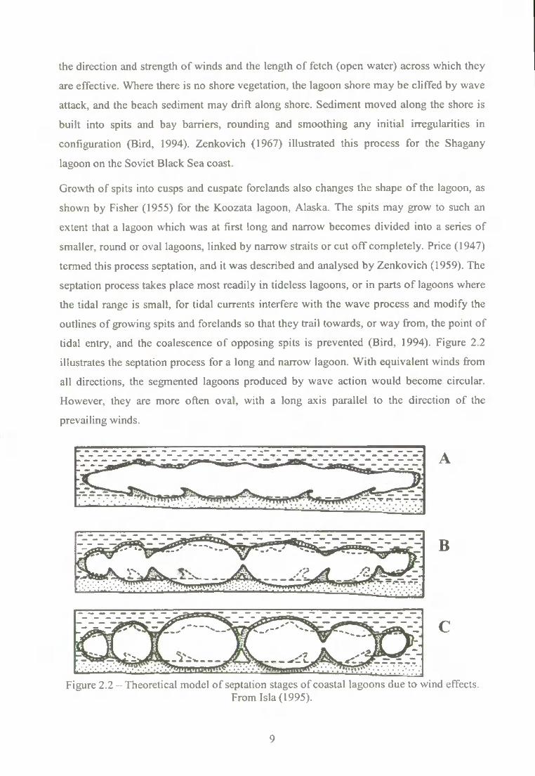
Growth of spits into cusps and cuspate forelands also changes the shape o f the lagoon, as
shown by Fisher (1955) for the Koozata lagoon, Alaska. The spits may grow to such an
extent that a lagoon which was at first long and narrow becomes divided into a series of
smaller, round or oval lagoons, linked by narrow straits or cut o f f completely. Price (1947)
termed this process septation, and it was described and analysed by Zenkovich (1959). The
septation process takes place most readily in tideless lagoons, or in parts o f lagoons where
the tidal range is small, for tidal currents interfere with the wave process and modify the
outlines of growing spits and forelands so that they trail towards, or way from, the point of
tidal entry, and the coalescence of opposing spits is prevented (Bird, 1994). Figure 2.2
illustrates the septation process for a long and narrow lagoon. With equivalent winds from
all directions, the segmented lagoons produced by wave action would become circular.
However, they are more often oval, with a long axis parallel to the direction of the
prevailing winds.
B
Figure 2.2 - Theoretical model of septation stages of coastal lagoons due to wind effects. From Isla(1995).
2.1.2. Circulation
The circulation o f a coastal lagoon, and thus mass transport processes, can be subdivided in
any of several ways (Smith, 1994). One o f the most basic distinctions is that of separating
tidal and non-tidal transport. Tidal currents are dependable and predictable because they
are periodic; thus they should be quantified in any comprehensive study of lagoon
circulation and water balance. Non-tidal circulation can be subdivided further by
distinguishing between barotropic and baroclinic forcing. A barotropic pressure gradient
arises from a slope in the surface o f the lagoon. Such a slope may in turn be created by the
wind driven set-up or set-down of water levels (seiche), or it may occur in response to
surface runoff entering the lagoon at some point. A baroclinic pressure gradient arises fi-om
density gradients resulting fi*om longitudinal and vertical salinity and/or temperature
gradients.
The circulation within a coastal lagoon can also be thought of as arising in response to
local and non-local (or remote) forcing. Local forcing is dominated by wind stress, which
generates currents, set-up and set-down (seiche) and short-period wind waves. Both tidal
and low frequency variations in coastal sea level result in the non-local forcing of the
lagoon circulation, manifested by oscillations with a period of 2 - 20 days, resulting in
either landward or seaward pressure gradients to aid in filling and emptying of the lagoons
(Knoppers & Kjerfve, 1999).
The measured flow within the lagoon at a given place and time may be a complex mix of
tidal and non-tidal currents, and at the same lime a response to both local and non-local
forcing. However, in lagoons with sufficiently restricted exchanges the local wind driven
circulation wi l l dominate all other forms o f locally or remotely forced non-tidal circulation
(Smith, 1994). An important feature of the local wind-driven current stems from the
seasonality in wind forcing. Seasonally changing wind patterns wi l l result in corresponding
changes in the wind driven circulation, and thus in net transport. It is common for wind
forcing to be stronger during autumn, winter and spring months, then decrease significantly
during summer months.
Local forcing by wind stress acting in confined water produces a laterally averaged direct
downwind transport regardless of the wind direction. The initial response wi l l be a set-up
of water levels along the downwind shore, a set-down along the upwind shore, and thus a
downwind directed slope in the free surface of the lagoon. Even for relatively light winds
10
of 5 - 10 m s"', the slope of the lagoon surface w i l l be on the order of 0.5 cm km' ' (Smith,
1994). The rise or fall in water level at the dovmwind and upwind ends o f the lagoon wi l l
be especially pronounced i f the lagoon is elongated and the wind direction parallels to the
longitudinal axis of the lagoon. The response to wind forcing can exceed the rise and fall
of the tide in a lagoon having restricted exchanges with shelf waters, and a longitudinal
axis on the order of several tens of kilometres. Csanady (1973) studied the formation of
surface and internal seiches in lakes as a response to imposed wind stress. He observed that
these seiches are usually dominated by unimodal modes, however Mortimer (1953)
observed 3 or 5 modes across Lake Michigan.
The secondary response to the wind and primary response to the barotropic pressure
gradient established by the set-up and set-down condition, is a downwind flow on the
surface and an upwind flow near the bed. The longitudinal barotropic gradient is supported
by depth-averaged stress but fiiction creates a vertical gradient leading to a return flow at
the bottom. Navigational channels may aid an upwind return flow. Both natural and man
made channels serve as conduits by locally expanding the layer between the downwind
directed wind stress itself, and the bottom fiictional force which resists the upwind return
flow. This has been discussed by Pitts (1989) for Florida's Indian River lagoon, and
modelled by Smith (1990). On the other hand, in shallow waters the return flow is at the
sides.
Because of the fundamental importance of lagoon-shelf exchanges, Kjerfve (1986) has
suggested the classification scheme described in Section 2.1.1. An understanding of
lagoon-shelf mass exchanges is important for two reasons. First, an active exchange of
water with the adjacent shelf has an important effect on lagoon hydrography and water
quality. Adjacent shelf waters are relatively stable in terms of temporal variability in
temperature and salinity. Exchanging water with the lagoon imports that stability and
reduces environmental extremes in the lagoon. This same exchange of water provides a
flushing effect, which maintains or restores water quality (Heam et ai, 1994). The second
reason involves the transport of migrating animal species. Shelf waters are the source of
much of the biota of lagoons, particularly the larval forms. Adult animals leaving the
lagoon nursery areas migrate seaward through inlets to live in continental shelf waters.
The forcing that affects lagoon-shelf exchanges is conceptually straightforward. Tidal
exchanges are forced by high and low water conditions occurring along the inner shelf, as
tidal waves of ocean basin scale move along the coast. Non-tidal exchanges occur when
11
coastal winds directly or indirectly raise or lower coastal sea level. The resulting inflow
and outflow from the lagoon is much like a tidal exchange, although it characteristically
occurs over time scales on the order of a week, as synoptic scale weather patterns move
through the study area.
Inlet morphology plays a central role in the lagoon-shelf exchange process (Smith, 1994).
First, because the constriction of an inlet acts as an exponential filter in the sense that the
damping effect it has on exchanges is directly related to the frequency of the rise and fall in
coastal sea level. For a sufficiently constricted inlet, tidal amplitudes in a lagoon may be
greatly reduced below amplitudes found nearby on the continental shelf Secondly, because
inlets condition sediment, salinity, nutrients, pollutant and organism dispersal between the
lagoon and the ocean (Isla, 1995).
2.2. About the Patos Lagoon
2.2.1. General aspects
Located in the southern Brazilian coastline between 30-32 °S and 50-52 *^V, the Patos
Lagoon (Figure 2.3) is the largest choked coastal lagoon in the world (Kjerfve, 1986). With
a length of 250 km and average width of 40 km, the lagoon has a surface area of 10,360
km^, and can be classified as a shallow lagoon since it has an average depth of 5 m. Depth
distribution along the lagoon is highly variable (Calliari, 1997). The bottom topography of
the main lagoon body is characterised by natural and artificial channels (8 - 9 m), large
adjacent areas (> 5 m), and shallow marginal bays. In the estuary, large shoal areas
between 1 and 5 m deep predominate, and maximum depth (18 m) is found at the inlet.
Many "cells" or "pools" limited by shallow sand spits mark the morphology of the Patos
Lagoon. This cellulju" shape formed because of the large area of the lagoon and the low
elevation of the surrounding dune-orientated topography. Zenkovich (1959) established
that when the wind blows parallel to such elongated lagoons, stationary waves produce
septation. For the Patos Lagoon septation, Toldo (1991) measured the growth of headlands
at a rate of 59.5 m year"'. However, he distinguished that those points on the western
margin are growing while those on the southern half of the eastern margin are eroding.
Thus it appears the spits may be at phase B on Figure 2.2.
12
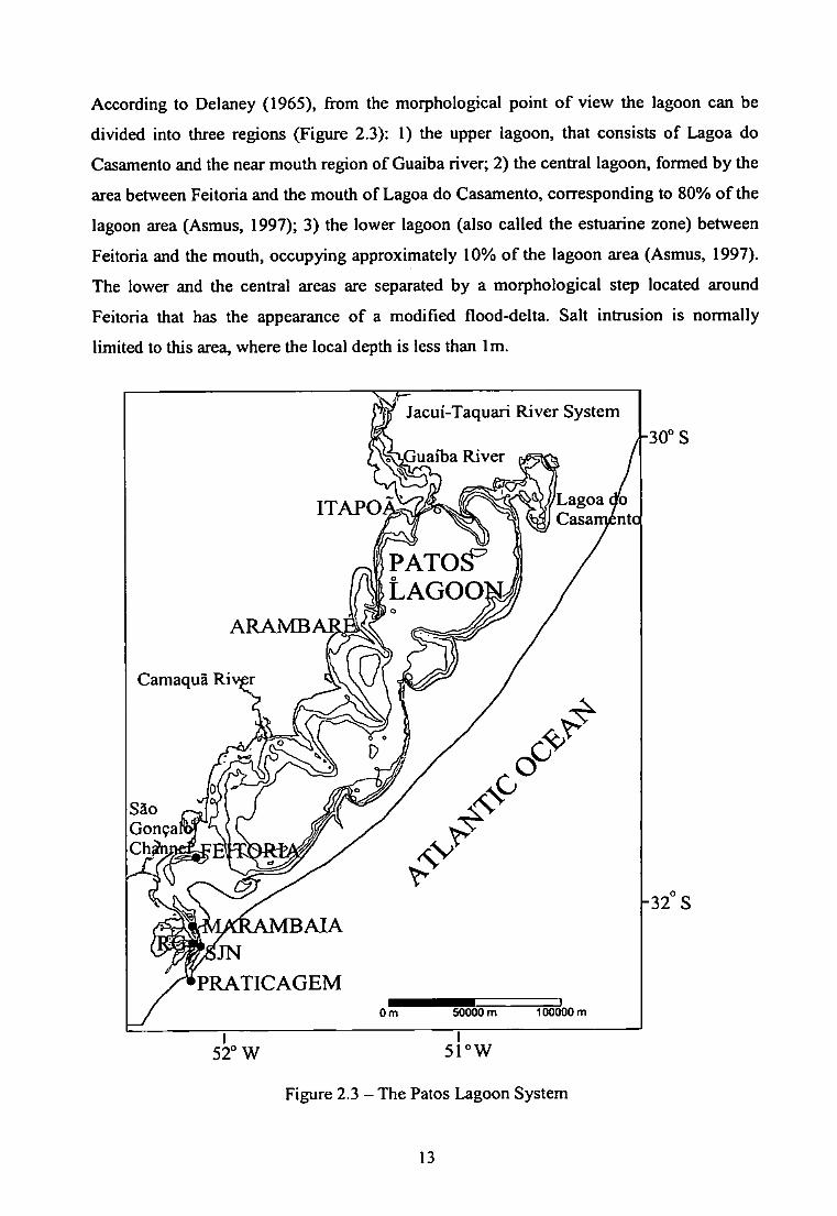
According to Delaney (1965), fi-om the morphological point of view the lagoon can be
divided into three regions (Figure 2.3): 1) the upper lagoon, that consists of Lagoa do
Casamento and the near mouth region of Guaiba river; 2) the central lagoon, formed by the
area between Feitoria and the mouth of Lagoa do Casamento, corresponding to 80% of the
lagoon area (Asmus, 1997); 3) the lower lagoon (also called the estuarine zone) between
Feitoria and the mouth, occupying approximately 10% of the lagoon area (Asmus, 1997).
The lower and the central areas are separated by a morphological step located around
Feitoria that has the appearance of a modified flood-delta. Sah intrusion is normally
limited to this area, where the local depth is less than Im.
ARAMB
Camaqua Ri
Jacui-Taquan River System
Guaiba River
ITAPO
L A G O O
AIA
P R A T I C A G E M
52" W
Sao Gon9a
50000 m 100000 m
30° S
32° S
5 1 ° W
Figure 2.3 - The Patos Lagoon System
13
2.2.2. Settlement and history
Prior to the arrival of the first European colonists, the indigenous Ghana and Tupi-Guarani
Indians occupied the southern Brazilian coastal plain (Asmus, 1997). The Indians settled
along the lagoon and ocean shores, where they exploited abundant fish, shellfish, and
shrimp resources (Vieira, 1983). The modem occupation history of the coastal plain began
with the arrival of politically opposed Portuguese and Spanish Jesuits in 1605 and 1626,
respectively. Following the Treaty o f Madrid in 1750, which ratified the agreement of
status quo after the foundation of the tov^ of Rio Grande in 1737, the coastal region
became the centre of intense Portuguese colonisation efforts. In order to reinforce its
diplomatic achievements and to warrant sovereignty, Portugal occupied the territory in
1747 with settlers fi^om the Azores, who entered through Rio Grande harbour. Colonisation
quickly radiated along the littoral towards Porto Alegre in the north and Chui in the south
(Figure 1.1).
From the very beginning, these seHlements not only exploited the abundant fishery
resources of the Patos Lagoon as a food source, but also used the lagoon as a cultural,
social, and commercial link. Advances in agricultural techniques, principally irrigated rice
cultivation, as well as the implementation of modem means of transport, caused profound
modifications in occupation and development of urban centres around the lagoon. Today,
virtually all port activities are assumed by the ports of Porto Alegre, Pelotas, and Rio
Grande, which move approximately 22,500,000 tons of goods every year (Asmus, 1997).
Over the last few decades, rapid and uncontrolled demographic and industrial growth
around the lagoon has altered its natural processes and magnified environmental conflicts.
Intense runoff from the Guaiba river tributaries is responsible for adding ever increasing
sediment loads, nutrients, hazardous heavy metals (Baisch et al, 1989), and agrotoxins.
Navigation and port activities and the establishment of fertiliser and fish processing plants
and petroleum refining have led to deterioration of the waters in the lower estuary
(Almeida a/., 1993).
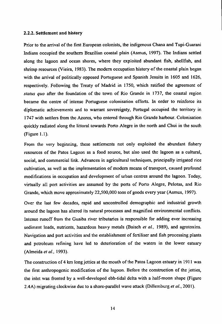
The construction of 4 km long jetties at the mouth of the Patos Lagoon estuary in 1911 was
the first anthropogenic modification o f the lagoon. Before the construction of the jetties,
the inlet was fronted by a well-developed ebb-tidal delta with a half-moon shape (Figure
2.4A) migrating clockwise due to a shore-parallel wave attack (Dillemburg et al., 2001),
14
The jetties were constructed by a French company as part of the regularisation of the
navigational channel (Motta, 1969). The construction promoted the transport of 14 million
m^ of sand to the ocean, which contributed for the formation of new sand banks at the end
of the jetties, the formation of an axial bank between the two jetties, which reduced the
navigational area and formed a double channel system (Figure 2.4B). It is difllcult to
establish the effect of this construction on the lagoon's circulation.
Figure 2.4 - Rio Grande channel bathymetric charts from 1885 (A) and 1988 (B). From Fetter (1999).
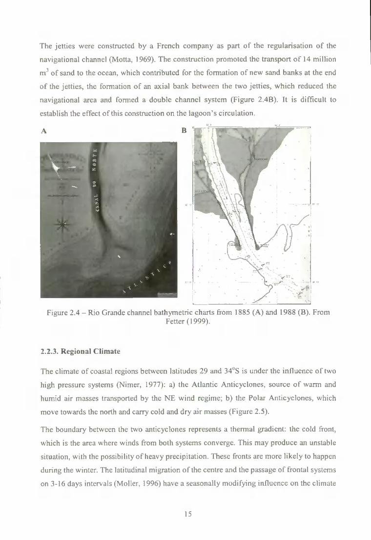
2.2.3. Regional Climate
The climate of coastal regions between latitudes 29 and 34''S is under the influence of two
high pressure systems (Nimer, 1977): a) the Atlantic Anticyclones, source of warm and
humid air masses transported by the NE wind regime; b) the Polar Anticyclones, which
move towards the north and carry cold and dry air masses (Figure 2.5).
The boundary between the two anticyclones represents a thermal gradient: the cold front,
which is the area where winds from both systems converge. This may produce an unstable
situation, with the possibility of heavy precipitation. These fronts are more likely to happen
during the winter. The latitudinal migration of the centre and the passage of frontal systems
on 3-16 days intervals (Moller, 1996) have a seasonally modifying influence on the climate
15
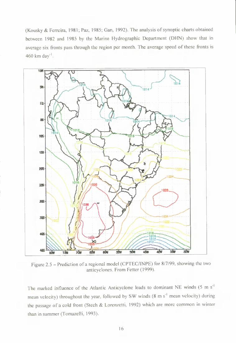
(Kousky & Ferreira, 1981; Paz, 1985; Gan, 1992). The analysis of synoptic charts obtained
between 1982 and 1985 by the Marine Hydrographic Department (DHN) show that in
average six fronts pass through the region per month. I he average speed of these fronts is
460 km day '.
Figure 2.5 - Prediction of a regional model (CPTEC/INPH) for 8/7/99, showing the two anticyclones. From Fetter (1999).
The marked influence of the Atlantic Anticyclone leads to dominant NE winds (5 m s '
mean velocity) throughout the year, followed by SW winds (8 m s"' mean velocity) during
the passage of a cold front (Stech & Lorenzetti, 1992) which are more common in winter
than in summer (Tomazelli, 1993).
16
The regional temperature regime is a function of season and number and intensity of cold
front passages (Nobre et ai, 1986). Mean annual temperatures vary between 19°C and
\TC in the north and south of the region, while monthly mean low and high temperatures
vary between 13°C and 24°C in July and January, respectively (IBGE, 1986). Total mean
annual precipitation (1200-1500 mm) may strongly vary from year to year and is mainly
related to the path and frequency of cold front passages (Gan, 1992). Mean monthly
rainfall is highest during the winter and spring (June to October), but a second peak may
occur in summer (Castello & Moller, 1978), when daily precipitation occasionally exceeds
100 mm (Gomes et ai, 1987). The summer months are associated with a seasonal water
deficit, although precipitation and evaporation result in an average annual water surplus of
200-300 mm (IBGE, 1986).
In the south-western Atlantic, distinct inter-annual variations in precipitation, with either a
high amount of rainfall or dry periods, seem to be a consequence of the El Nifto-Southem
Oscillation cycle on the global climate (Nobre et al., 1986; Gan, 1992), but the processes
involved are still not well understood. This phenomenon directly influences the amount of
continental freshwater runoff and thus the biogeochemical processes in coastal and marine
ecosystems of the Southwest Atlantic (Ciotti et ai, 1995).
2,2.4. River Flow
The rivers that flow into the lagoon have a total catchment area of 201,626 km^. They
exhibit a typical mid-latitude pattern of high discharge in late winter and early spring,
followed by low to moderate discharge through summer and autumn. They also have a
large year-to-year variation in discharge (Moller, 1996). Each part of the lagoon has its
own tributaries (Figure 2.3). In the northern region, the main tributary is the Guaiba River,
which receives freshwater from the Jacui'-Taquari river system and is responsible for 85 %
of the average total freshwater input in the lagoon. In the central region, the main tributary
is the Camaqui River, responsible for the remaining 15 % of the freshwater discharge. In
the estuarine region the Patos Lagoon connects to the South Atlantic Ocean via a channel
20 km long and 1 km wide. In the middle area of the estuary, the Sao Gongalo Channel
connects the Patos Lagoon to the Mirim Lagoon (surface area of 3,749 km^), forming the
Patos-Mirim system.
The freshwater discharge is a very important factor in the formation of longitudinal salinity
gradients during mixing processes, which represent the baroclinic part of the lagoon
17
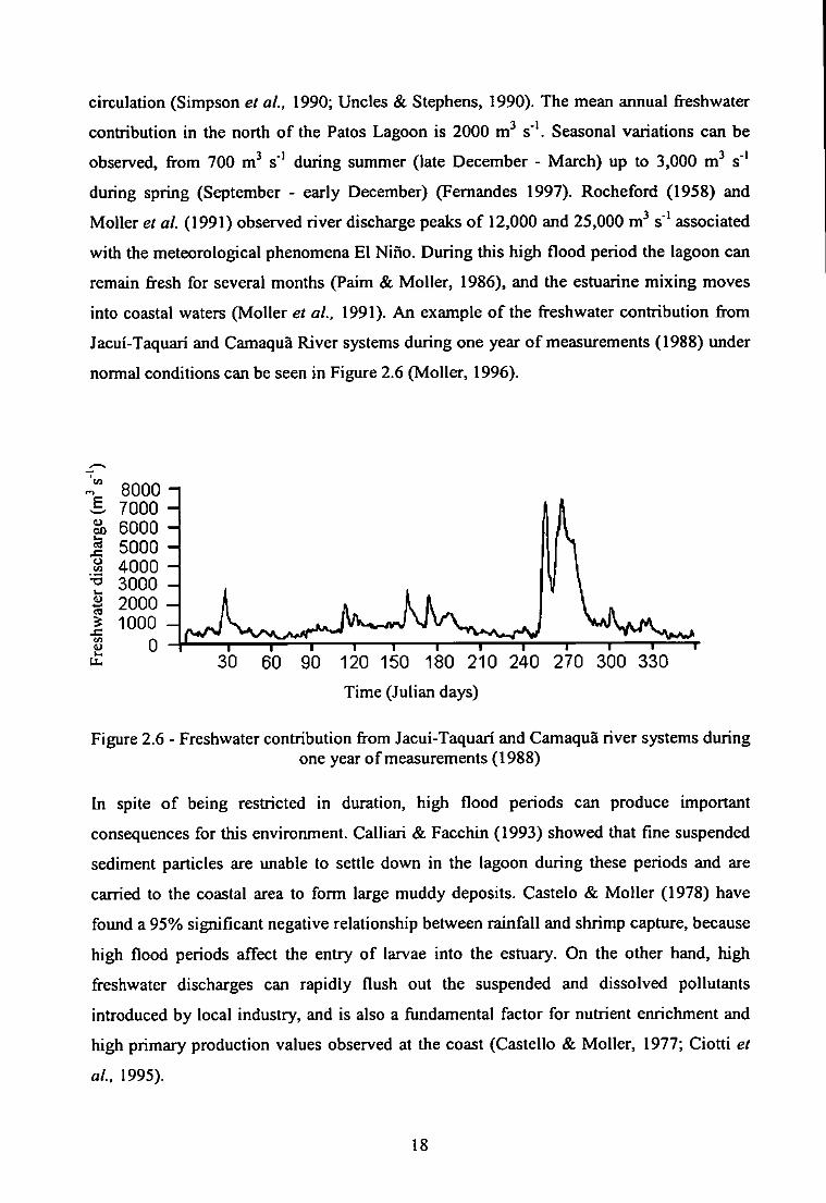
circulation (Simpson et ai, 1990; Uncles & Stq)hens, 1990). The mean annual freshwater
contribution in the north of the Patos Lagoon is 2000 m"* s'*. Seasonal variations can be
observed, from 700 m^ s" during summer (late December - March) up to 3,000 m"* s *
during spring (September - early December) (Femandes 1997). Rocheford (1958) and
MoUer et ai (1991) observed river discharge peaks of 12,000 and 25,000 m^ s ' associated
with the meteorological phenomena El Nino. During this high flood period the lagoon can
remain fresh for several months (Paim & Moller, 1986), and the estuarine mixing moves
into coastal waters (Moller et ai, 1991). An example of the freshwater contribution from
Jacui-Taquari and Camaqua River systems during one year of measurements (1988) under
normal conditions can be seen in Figure 2.6 (Moller, 1996).
8000 - I ^ 7000 -S) 6000 -I 5000 -a 4000
CO
SI
3000 2000 1000
0 30 60 90 120 150 180 210 240 270 300 330
Time (Julian days)
Figure 2.6 - Freshwater contribution from Jacui-Taquari and Camaqua river systems during one year of measurements (1988)
In spite of being restricted in duration, high flood periods can produce important
consequences for this environment. Calliari & Facchin (1993) showed that fine suspended
sediment particles are unable to settle down in the lagoon during these periods and are
carried to the coastal area to form large muddy deposits. Castelo & MoHer (1978) have
found a 95% significant negative relationship between rainfall and shrimp capture, because
high flood periods affect the entry of larvae into the estuary. On the other hand, high
freshwater discharges can rapidly flush out the suspended and dissolved pollutants
introduced by local industry, and is also a ftmdamental factor for nutrient enrichment and
high primary production values observed at the coast (Castello & Moller, 1977; Ciotti et
aL 1995).
18
2.2.5. Tidal forcing and wind effect
Wang & Elliot (1978), Wang (1979), Wang & Garvine (1984) observed that in coastal
lagoons the relative importance of the wind in the system circulation increases as the tidal
amplitude decreases. Smith (1980) and Kjerfve & Knoppers (1991) explained that this
happens because the tidal amplitude is attenuated by the shear stress created in the narrow
channel. This is the case on the Patos Lagoon, located in a region of minimum tidal
influence (Defant, 1961). The estuary is microtidal and tides are mixed mainly of the
diurnal type, with mean tidal amplitude of 0.47 m and Form Number of 2.42 (Garcia,
1997). The principal tidal constituent Oi (period 25.8h) has an amplitude of 10.8 cm (Herz,
1977). The dynamics are therefore essentially dependent on the wind and on the freshwater
discharge (Malaval, 1922; Motta, 1969; Kjerfve, 1986; MoUer et al, 1991; Moller et al,
1996; Femandes et al., in press a). According to Garcia (1997), maximum current
velocities in the main lagoon body are about 30 cm s ', with a frequent inversion of
direction, however, in the inlet flushing current velocities may reach 1.7 - 1.9 m s"' after
prolonged periods of heavy rainfall (DNPVN, 1941).
The local wind was identified as the principal forcing factor in the Patos Lagoon system in
the past (Malaval, 1922), although the wind drives the lagoon circulation through both
local and non- local effects. Northeasterly (NE) winds are dominant throughout the year.
During summer and spring there is also a well-marked preference of easterly (E) winds,
indicating the influence of sea breezes (Moller, 1996). Southwesterly (SW) winds become
more important during autumn and winter as frontal systems become more frequent over
this area. According to Tomazelli (1993), at Rio Grande City (Figure 2.3) 22.3% of the
observations between 1970 and 1982 indicated the presence of NE winds, and 13.5% of
SW winds. Typical wind speeds are between 3-5 m s"' (Femandes, 1997).
The wind action in the Patos Lagoon can be observed through the difference in level
generated inside the lagoon and between the lagoon and the ocean. These are the factors
responsible for the input and output of oceanic water, in spite of the different water masses
that controls the coastal system. Under normal flow conditions, river input controls the
mean lagoon water level, which is modulated by the wind. The freshwater discharge
produces a super-elevation (Mehta, 1990) that SW winds will have to overcome in order to
force salt water to enter into the system. During periods of high fluvial discharge, only
19
stormy conditions can reverse the pressure gradient developed between the lagoon and the
coastal area.
As a consequence of reduced fidal influence in the inlet and in the estuary, the salinity
distribution lacks tidal variability but does correlate with wind forcing and variations in
freshwater input on scales of hours to weeks (Garcia, 1997). During periods of low
discharge (summer and autimin), onshore SE and SW winds force seawater through the
inlet into the lower estuary and occasionally as far as 150 km into the lagoon, hi contrast,
NE winds together with high fluvial discharge significantly decrease estuarine salinity
(Calliari. 1980; Costa et ai, 1988). Fluvial discharge in excess of 3000 m"* s ' causes
pronounced salinity stratification in the inlet, and higher values extend the estuarine
mixing zone into coastal waters (Moller et al., 1991). AJthough our understanding of the
system's hydrodynamics is still limited, it is evident that both the regional climate and the
hydrological cycles are the principal forcing factors controlling the lagoon and estuarine
circulation patterns and salinity variations.
A. Tidal forcing
Moller et al. (1996) studied the summertime response of the Patos Lagoon to the wind and
astronomical tidal forcing. This study was carried out through the analysis of time series of
field data and from the results of a two-dimensional numerical model of the barotropic
circulation (Wang & Connor, 1975).
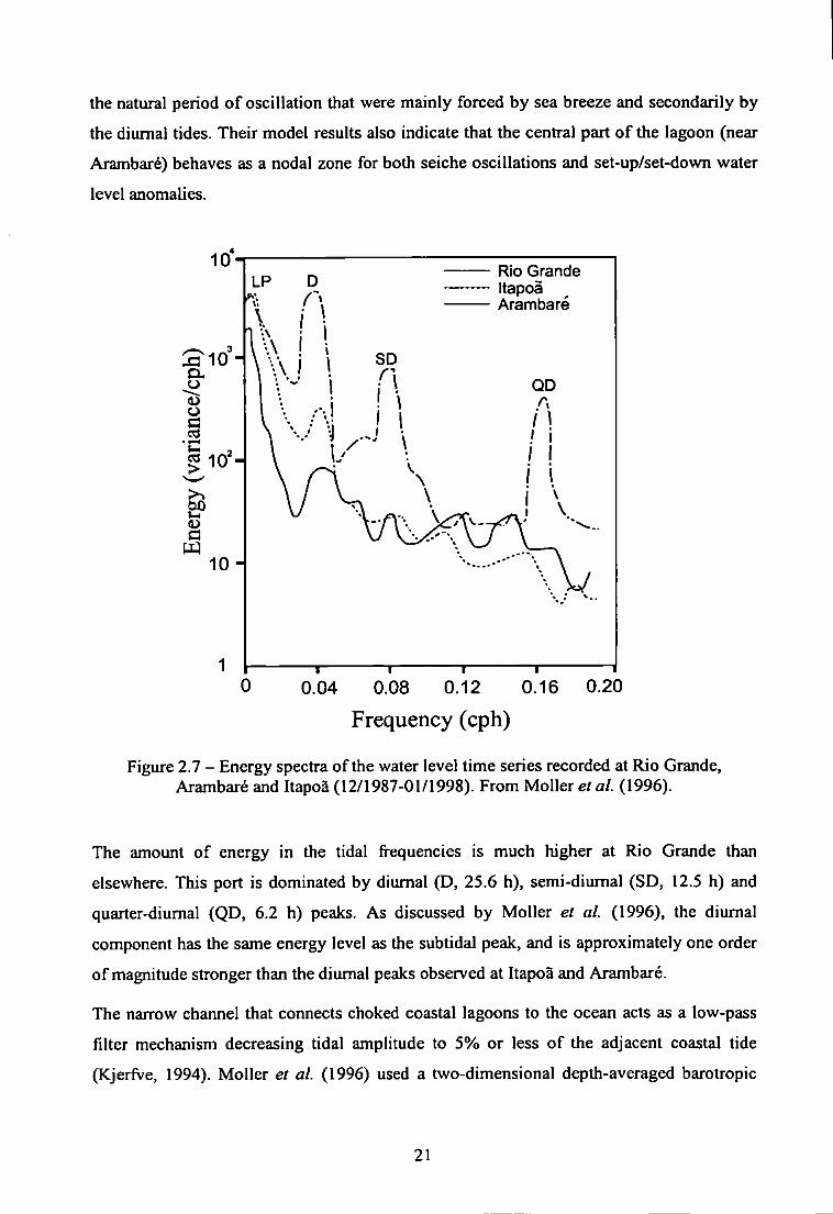
Figure 2.7 shows the energy spectrum of individual time series determined through the
FFT technique applied on unfiltered water level oscillations for Rio Grande (extreme south
of the domain), Arambare (middle part of the lagoon), and Itapoa (extreme north of the
lagoon). The longitudinal component of the wind proved to be the main mechanism
responsible for the water level oscillations throughout the lagoon at the low frequency end
of the spectrum (0.0039 cph). The response of the lagoon to this longitudinal wind forcing
was found to be of the set-up/set-down type, where the piling up of water occurs
downwind.
The two diurnal peaks observed at Itapoa and Arambare are unlikely to be of tidal origin,
because they are far away from the entrance channel. Moller et al. (1996) found high
coherence between the sea breeze signal and the water level in this 24 hours period band.
Moller (1996) concluded that these 24 hour water level oscillations were seiches related to
20
the natural period of oscillation that were mainly forced by sea breeze and secondarily by
the diurnal tides. Their model results also indicate that the central part of the lagoon (near
Arambare) behaves as a nodal zone for both seiche oscillations and set-up/set-down water
level anomalies.
10'
43 10H
10
Rio Grande Itapoa Arambare
0 — I — 0.04 0.08 0.12 0.16
Frequency (cph) 0.20
Figure 2.7 - Energy spectra of the water level time series recorded at Rio Grande, Arambare and Itapoa (12/1987-01/1998). From Moller et al (1996).
The amount of energy in the tidal frequencies is much higher at Rio Grande than
elsewhere. This port is dominated by diurnal (D, 25.6 h), semi-diurnal (SD, 12.5 h) and
quarter-diumal (QD, 6.2 h) peaks. As discussed by Moller et al (1996), the diurnal
component has the same energy level as the subtidal peak, and is approximately one order
of magnitude stronger than the diurnal peaks observed at Itapoa and Arambare.
The narrow channel that connects choked coastal lagoons to the ocean acts as a low-pass
filter mechanism decreasing tidal amplitude to 5% or less of the adjacent coastal tide
(Kjerfve, 1994). Moller et al. (1996) used a two-dimensional depth-averaged barotropic
21
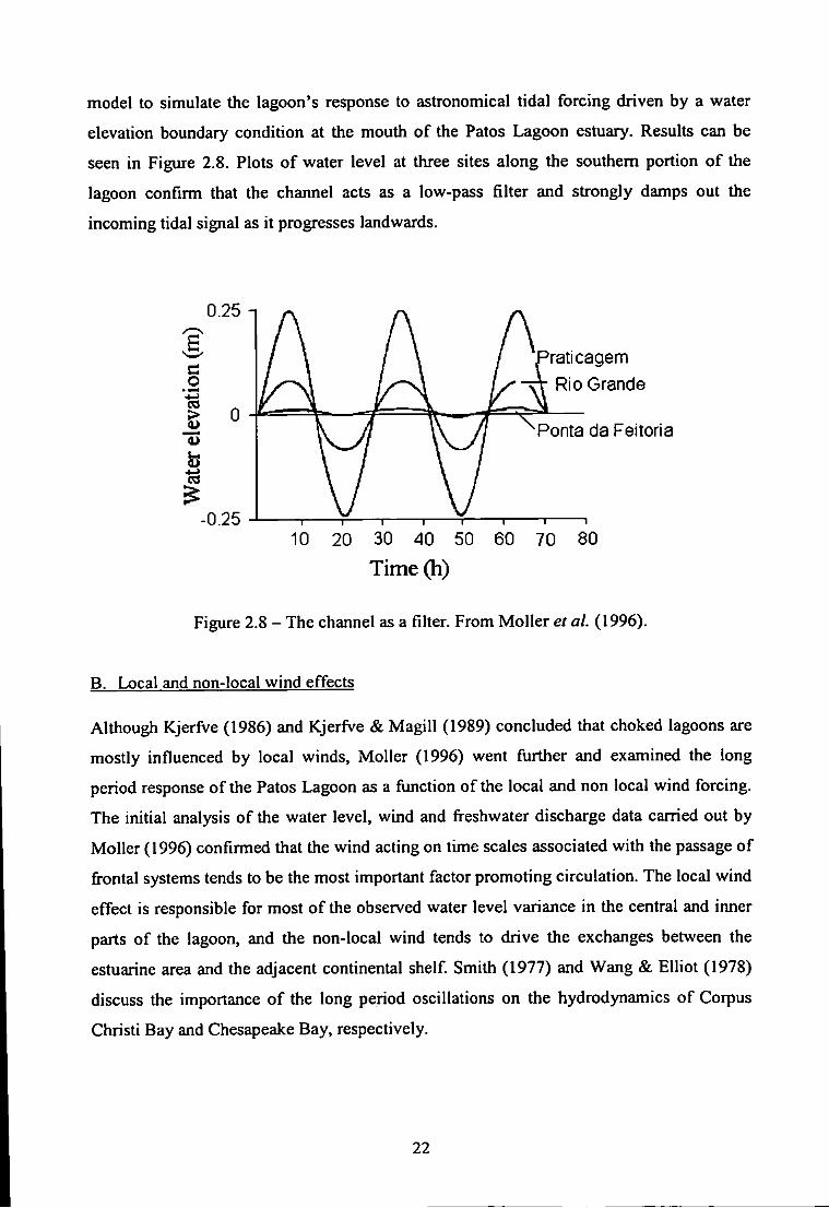
model to simulate the lagoon's response to astronomical tidal forcing driven by a water
elevation boundary condition at the mouth of the Patos Lagoon estuary. Results can be
seen in Figure 2.8. Plots of water level at three sites along the southern portion of the
lagoon confirm that the channel acts as a low-pass filter and strongly damps out the
incoming tidal signal as it progresses landwards.
0.25 n
o
C4
0.25
raticagem Rio Grande
Ponta da Feitoria
10 20 30 40 50 60 70 80 Time (h)
Figure 2.8 - The channel as a filter. From Moller et al. (1996).
B. Local and non-local wind effects
Although Kjerfve (1986) and Kjerfve & Magill (1989) concluded that choked lagoons are
mostly influenced by local winds, Moller (1996) went fiirther and examined the long
period response of the Patos Lagoon as a function of the local and non local wind forcing.
The initial analysis of the water level, wind and freshwater discharge data carried out by
Moller (1996) confirmed that the wind acting on time scales associated with the passage of
frontal systems tends to be the most important factor promoting circulation. The local wind
effect is responsible for most of the observed water level variance in the central and inner
parts of the lagoon, and the non-local wind tends to drive the exchanges between the
estuarine area and the adjacent continental shelf Smith (1977) and Wang & Elliot (1978)
discuss the importance of the long period oscillations on the hydrodynamics of Corpus
Christi Bay and Chesapeake Bay, respectively.
22
In order to understand the real effect of these forces on the estuarine area of the Patos
Lagoon, several experiments were carried out (Moller, 1996) using the coupled two-
dimensional and three-dimensional model formulated by Lazure & Salomon (1991). The
two models together form a coherent system which permits a three-dimensional calculation
in areas where this is absolutely necessary, obviously with higher costs. Lazure and
Salomon observed that the coupling of these models is not simple and may decrease the
stability of the system.
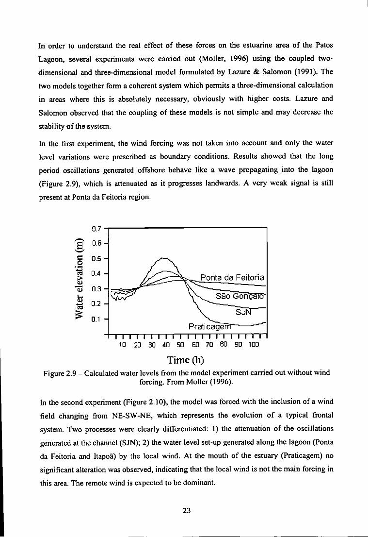
In the first experiment, the wind forcing was not taken into account and only the water
level variations were prescribed as boundary conditions. Results showed that the long
period oscillations generated offshore behave like a wave propagating into the lagoon
(Figure 2.9), which is attenuated as it progresses landwards. A very weak signal is still
present at Ponta da Feitoria region.
0.7
Ponta da Feitoria
Sao Gorigalo
Praticagei I I I I I I I I I I I I I I I I I I I I I 10 20 30 40 50 H] 70 80 90 100
Time(h) Figure 2.9 - Calculated water levels from the model experiment carried out without wind
forcing. From Moller (1996).
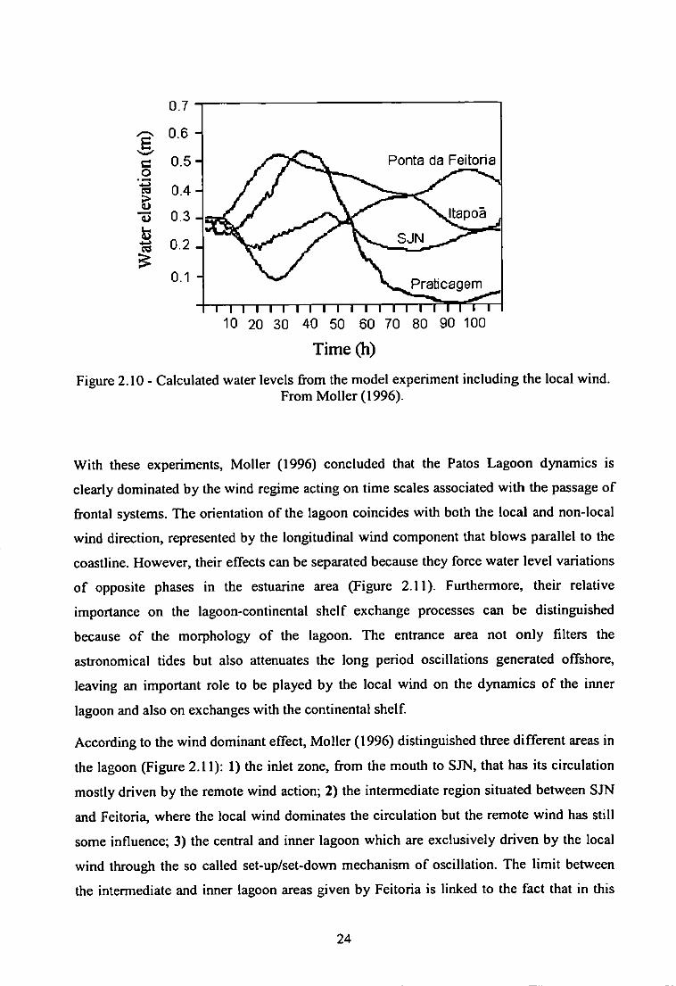
In the second experiment (Figure 2.10), the model was forced with the inclusion of a wind
field changing from NE-SW-NE, which represents the evolution of a typical frontal
system. Two processes were clearly differentiated: 1) the attenuation of the oscillations
generated at the channel (SJN); 2) the water level set-up generated along the lagoon (Ponta
da Feitoria and Itapoa) by the local wind. At the mouth of the estuary (Praticagem) no
significant alteration was observed, indicating that the local wind is not the main forcing in
this area. The remote wind is expected to be dominant.
23
0.7
c o
a> s
Ponta da Feitoria
0.6 H
Itapoa
0.1 H Prabcagem I I I 1 I I I I I I I I I i i i I I I I
10 20 30 40 50 60 70 80 90 100
Time (h)
Figure 2.10 - Calculated water levels from the model experiment including the local wind. From Moller (1996).
With these experiments, Moller (1996) concluded that the Patos Lagoon dynamics is
clearly dominated by the wind regime acting on time scales associated with the passage of
frontal systems. The orientation of the lagoon coincides with both the local and non-local
wind direction, represented by the longitudinal wind component that blows parallel to the
coastline. However, their effects can be separated because they force water level variations
of opposite phases in the estuarine area (Figure 2.11). Furthennore, their relative
importance on the lagoon-continental shelf exchange processes can be distinguished
because of the morphology of the lagoon. The entrance area not only filters the
astronomical tides but also attenuates the long period oscillations generated offshore,
leaving an important role to be played by the local wind on the dynamics of the inner
lagoon and also on exchanges with the continental shelf
According to the wind dominant effect, Moller (1996) distinguished three different areas in
the lagoon (Figure 2.11): 1) the inlet zone, from the mouth to SIN, that has its circulation
mostly driven by the remote wind action; 2) the intermediate region situated between SJN
and Feitoria, where the local wind dominates the circulation but the remote wind has still
some influence; 3) the central and inner lagoon which are exclusively driven by the local
wind through the so called set-up/set-down mechanism of oscillation. The limit between
the intermediate and inner lagoon areas given by Feitoria is linked to the fact that in this
24
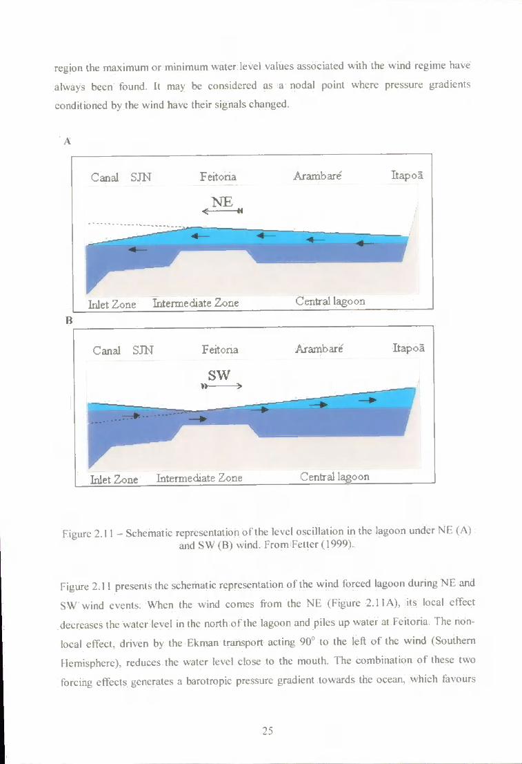
region the maximum or minimum water level values associated with the wind regime have
always been found. It may be considered as a nodal point where pressure gradients
conditioned by the wind have their signals changed.
Canal SJN Feitona Arambare ItapoS
N E < «
^ ^ ^ ^ ^ ^ ^ •
Inlet Zone Intermediate Zone Central lagoon
Canal SJN Feitona Arambare I t ^ o a
Inlet Zone Intermediate Zone Central lagoon
Figure 2.11 - Schematic representation of the level oscillation in the lagoon under NE (A) and SW (B) wind. From Fetter (1999).
Figure 2.11 presents the schematic representation of the wind forced lagoon during NE and
SW wind events. When the wind comes from the NE (Figure 2.11 A), its local effect
decreases the water level in the north of the lagoon and piles up water at Feitoria. The non
local effect, driven by the Ekman transport acting 90" to the lef of the wind (Southern
Hemisphere), reduces the water level close to the mouth. The combination of these two
forcing effects generates a barotropic pressure gradient towards the ocean, which favours
25
flushing of the lagoon water. When the wind comes from the SW (Figure 2.1 IB), its local
effect increases the water level in the north of the lagoon and decreases at Feitoria, and the
non-local effect driven by the Ekman transport is now piling up water close to the mouth.
The combination of both effects generates a barotropic pressure gradient towards Feitoria,
which favours water penetration into the lagoon. This mechanism, which combines the
non-Iocal and local wind action, is the most important factor that forces exchanges between
the lagoon and the continental shelf The stronger the wind the more important the pressure
gradient established between the coast and Feitoria region, and the magnitude of water
advection into or out of the lagoon. Femandes & Niencheski (1998) calculated horizontal
advective fluxes ranging between 1x10"* and IxlO'* m"* s"' for the estuary under the
influence of NE and SW winds using a simple box model (Femandes, 1997).
26
Chapter 3
Description of the iieldwork
3.1. Introduction
In the past decade, numerical modelling has been used to study the wind-driven
circuladon, as well as the tidal and subtidal effects, on the Patos Lagoon hydrodynamics
(Moller et al., 1991; Moller et a/., 1996; Moller, 1996; Moller & Castaing, 1999;
Femandes et al., in press a, b, c). However, modelling consists of numerical solutions
using reasonable approximations to the basic governing equations, where a common area
of weakness is the paucity of suitable data to support the numerical models and to verify
the validity of the approximations (Cheng & Walters, 1982).
Field measurements were carried out on Patos Lagoon estuary in order to generate data to
support the modelling study. Between 27-29/10/1998, measurements were simultaneously
carried out in the channel area at Praticagem, Marambaia and Feitoria stations (Figure 3.1).
Similar measurements were carried out in the shallow area at Porto Rei station (Figure 3.1)
between 05-06/11/1998. Although field measurements along the lagoon would be
recommended, limitations involving the size of the lagoon, the cost of personnel and
shortage of equipment have concentrated measurements in the estuarine area.
3.2. Fieldwork strategy
The Patos Lagoon estuary experiences great spatial variations, seasonal, tidal and subtidal
oscillations in material concentrations, water level and flow velocity. This is primarily due
to the combination of inflow of fi*eshwater, meteorological forcing (wind and pressure
variation), small tidal influence, and constraints imposed by the configuration and geology
of the estuary. Thus, the representativeness of any set of estuarine measurements is highly
dependent on the sampling design. Location of stations, total number of stations, and the
number of vertical measurements per station should be carefully selected (Kjerfve, 1979).
Large areas of shallow water cut by channels dominate the estuarine morphology. As these
features have different hydrodynamic behaviour, an ideal sampling design should involve
measurements in both areas. However, such design would involve resources that were not
27
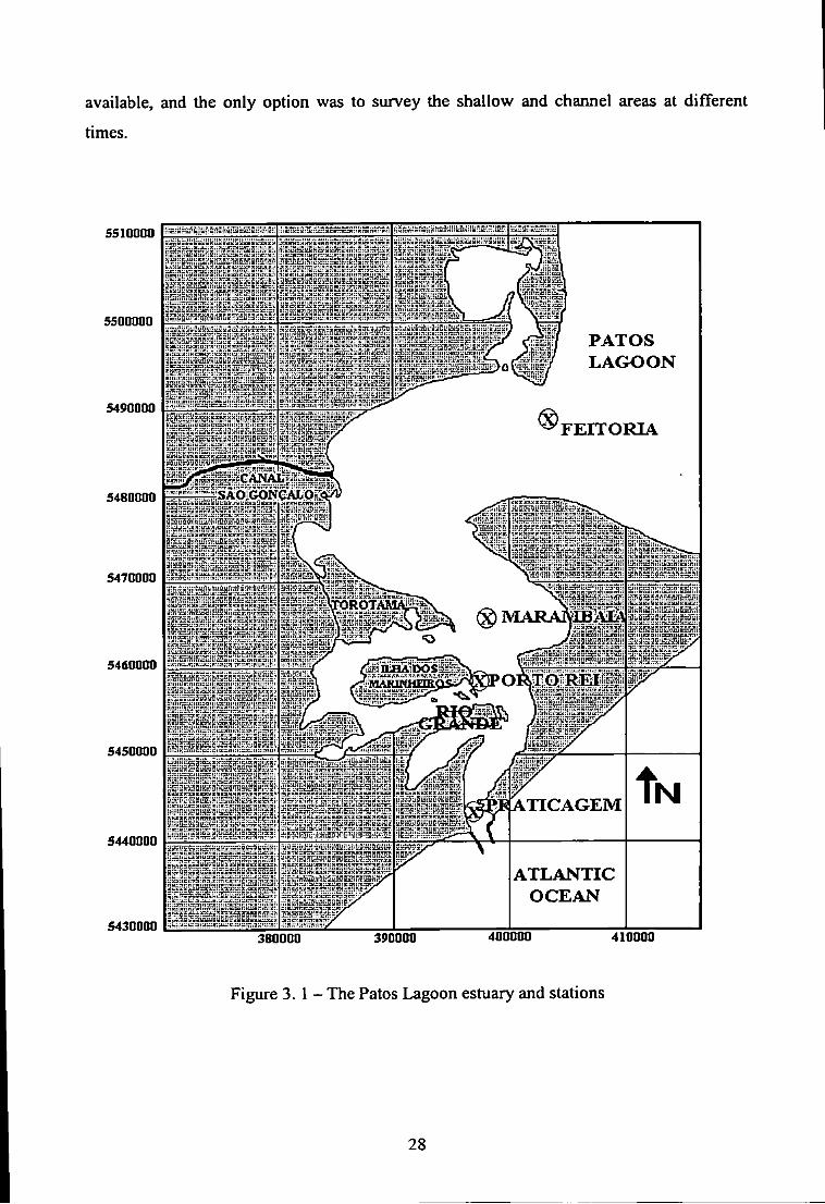
available, and the only option was to survey the shallow and channel areas at different
times.
5510000
5500000
5490000
5480000
5470000
5460000
5450000
5440000
5430000
• SB H Mlf KM • M i t
K ; 7K;: tt-vn r.n^ E : : a: :s - 1 ^ 31 Oiiain :r.ji',mnHXn^KKat<ar.it
mi j l i : c 1 ijjau i 1:1 IK11! : i : =: c:; • :.-»ne
fJ-K K inu := : i : : K^sci 11: TI: v ^ - i l 1 Hi: :e
I: K a: III 1 :iet »i:i:i:mi I u ( Fi: I u K »3 PATOS L A G O O N
\NAL GONCAf
£:S,•"•'S 4f=fi3S.! S! l!|E! >d!!Ti:iuiain:iiii»:
f.str.n-^tii^-.-.iKijn
:>=;iii;::i:s;ni:;i!Sii::ii;:;
TOROT
A T L A N T I C O C E A N
380000 390000 400000 410000
Figure 3 . 1 - The Patos Lagoon estuary and stations
28
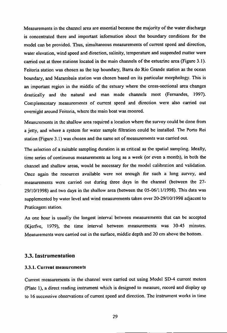
Measurements in the channel area are essential because the majority of the water discharge
is concentrated there and important information about the boundary conditions for the
model can be provided. Thus, simultaneous measurements of current speed and direction,
water elevation, wind speed and direction, salinity, temperature and suspended matter were
carried out at three stations located in the main channels of the estuarine area (Figure 3.1).
Feitoria station was chosen as the top boundary, Barra do Rio Grande station as the ocean
boundary, and Marambaia station was chosen based on its particular morphology. This is
an important region in the middle of the estuary where the cross-sectional area changes
drastically and the natural and man made charmels meet (Femandes, 1997).
Complementary measurements of current speed and direction were also carried out
overnight around Feitoria, where the main boat was moored.
Measurements in the shallow area required a location where the survey could be done from
a jetty, and where a system for water sample filtration could be installed. The Porto Rei
station (Figure 3.1) was chosen and the same set of measurements was carried out.
The selection of a suitable sampling duration is as critical as the spatial sampling. Ideally,
time series of continuous measurements as long as a week (or even a month), in both the
channel and shallow areas, would be necessary for the model calibration and validation.
Once again the resources available were not enough for such a long survey, and
measurements were carried out during three days in the channel (between the 27-
29/10/1998) and two days in the shallow area (between the 05-06/11/1998). This data was
supplemented by water level and wind measurements taken over 20-29/10/1998 adjacent to
Praticagem station.
As one hour is usually the longest interval between measurements that can be accepted
(Kjerfve, 1979), the time interval between measurements was 30-45 minutes.
Measurements were carried out in the surface, middle depth and 20 cm above the bottom.
3.3. Instrumentation
3.3.1. Current measurements
Current measurements in the channel were carried out using Model SD-4 current meters
(Plate 1), a direct reading instrument which is designed to measure, record and display up
to 16 successive observations of current speed and direction. The instrument works in time
29
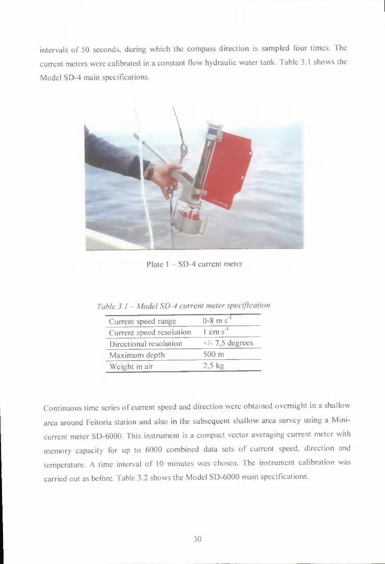
intervals of 50 seconds, during which the compass direction is sampled four limes. The
current meters were calibrated in a constant flow hydraulic water tank. Table 3.1 shows the
Model SD-4 main specifications.
Plate 1 - SD-4 current meter
Table 3.1 Model SD-4 current meter specification
Current speed range 0-8 m s ' Current speed resolution 1 cm s ' Directional resolution -»-/- 7.5 degrees Maximum depth 500 m Weight in air 2,5 kg
Continuous time series of current speed and direction were obtained overnight in a shallow
area around Feitoria station and also in the subsequent shallow area survey using a Mini-
current meter SD-6000. This instrument is a compact vector averaging current meter with
memory capacity for up to 6000 combined data sets of current speed, direction and
temperature. A time interval of 10 minutes was chosen. The instrument calibration was
carried out as before. Table 3.2 shows the Model SD-6000 main specifications.
30
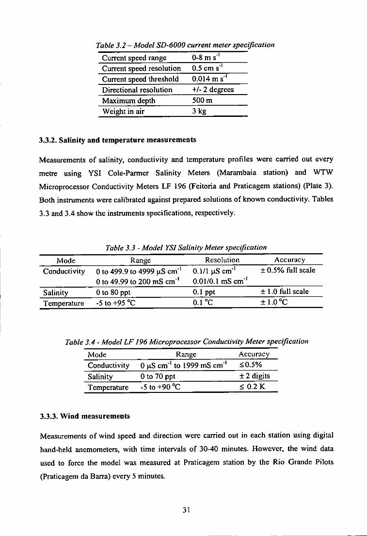
Table 3.2- Model SD-6000 current meter specification
Current speed range 0-8 m s* Current speed resolution 0.5 cm s"' Ciurent speed threshold 0.014 ms'* Directional resolution +/- 2 degrees Maximum depth 500 m Weight in air 3 kg
3.3.2. Salinity and temperature measurements
Measurements of salinity, conductivity and temperature profiles were carried out every
metre using YSI Cole-Parmer Salinity Meters (Marambaia station) and WTW
Microprocessor Conductivity Meters LF 196 (Feitoria and Praticagem stations) (Plate 3).
Both instruments were calibrated against prepared solutions of known conductivity. Tables
3.3 and 3.4 show the instruments specifications, respectively.
Table 3.3 - Model YSI Salinity Meter specification
Mode Range Resolution Accuracy Conductivity 0 to 499.9 to 4999 jiS cm"
Oto 49.99 to 200 mS cm * 0.1/1 nS cm"' 0.01/0.1 mS cm"'
± 0.5% frill scale
Salinity 0 to 80 ppt 0.1 ppt ± 1.0 frill scale Temperature -5 to +95 °C 0.1 °C l l .O^'C
Table 3.4 - Model LF 196 Microprocessor Conductivity Meter specification
Mode Range Accuracy Conductivity 0 (iS cm ' to 1999 mS cm ' <0.5% Salinity 0 to 70 ppt ± 2 digits Temperature -5 to +90 °C < 0.2 K
3.3.3. Wind measurements
Measurements of wind speed and direction were carried out in each station using digital
hand-held anemometers, with time intervals of 30-40 minutes. However, the wind data
used to force the model was measured at Praticagem station by the Rio Grande Pilots
(Praticagem da Barra) every 5 minutes.
31
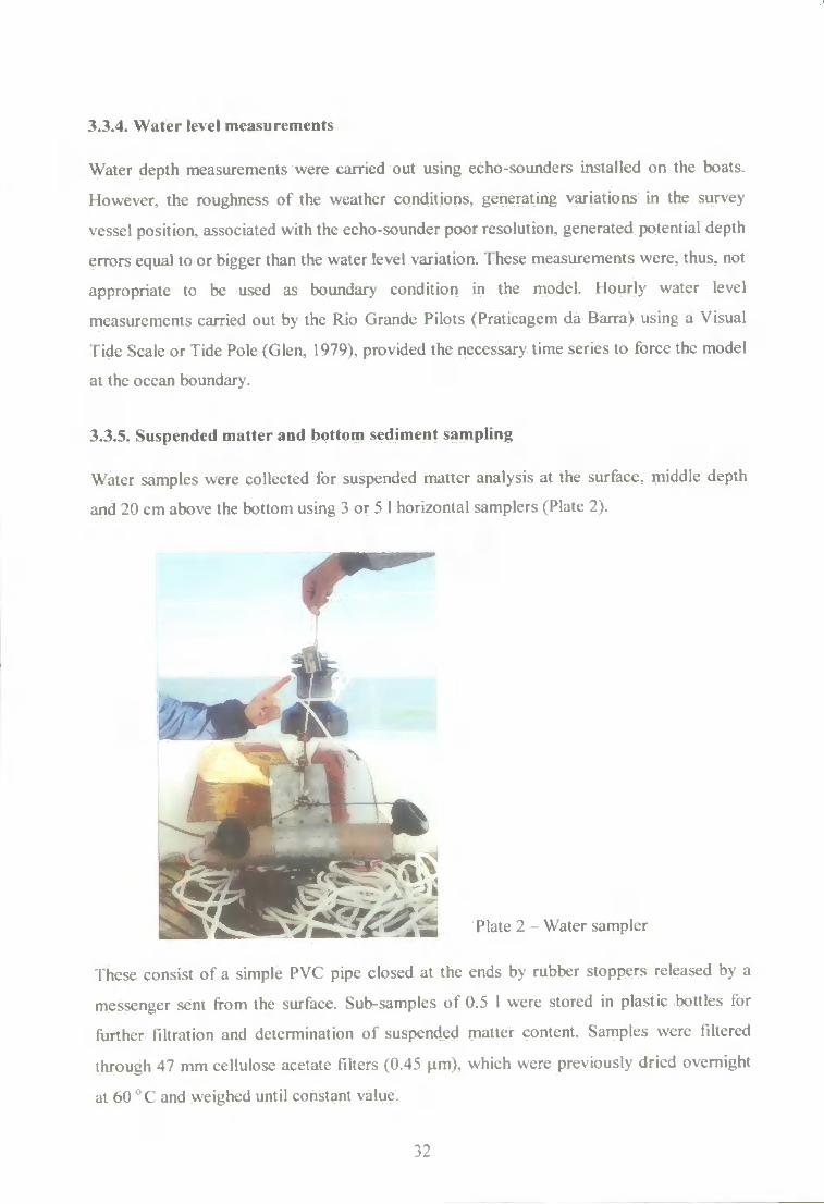
3.3.4. Water level measurements
Water depth measurements were carried out using echo-sounders installed on the boats.
However, the roughness of the weather conditions, generating variations in the survey
vessel position, associated with the echo-sounder poor resolution, generated potential depth
errors equal to or bigger than the water level variation. These measurements were, thus, not
appropriate to be used as boundary condition in the model. Hourly water level
measurements carried out by the Rio Grande Pilots (Praticagem da Barra) using a Visual
ride Scale or Tide Pole (Glen, 1979), provided the necessary time series to force the model
at the ocean boundary.
3.3.5. Suspended matter and bottom sediment sampling
Water samples were collected for suspended matter analysis at the surface, middle depth
and 20 cm above the bottom using 3 or 5 1 horizontal samplers (Plate 2).
Plate 2 - Water sampler
These consist of a simple PVC pipe closed at the ends by rubber stoppers released by a
messenger sent from the surface. Sub-samples of 0.5 1 were stored in plastic bottles for
further filtration and determination of suspended matter content. Samples were filtered
through 47 mm cellulose acetate filters (0.45 |im). which were previously dried overnight
at 60 '*C and weighed until constant value.
32
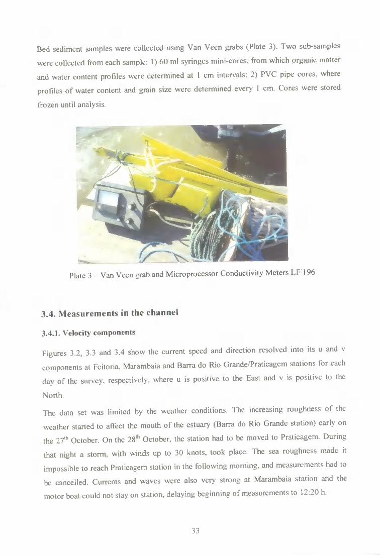
Bed sediment samples were collected using Van Veen grabs (Plate 3). Two sub-samples
were collected from each sample: 1) 60 ml syringes mini-cores, from which organic matter
and water content profiles were determined at 1 cm intervals; 2) PVC pipe cores, where
profiles of water content and grain size were determined every 1 cm. Cores were stored
frozen until analysis.
Plate 3 - Van Veen grab and Microprocessor Conductivity Meters LF 196
3.4. Measurements in the channel
3.4.1. Velocity components
Figures 3.2, 3.3 and 3.4 show the current speed and direction resolved into its u and v
components at Feitoria, Marambaia and Barra do Rio Grande/Praticagem stations for each
day of the survey, respectively, where u is positive to the East and v is positive to the
North.
The data set was limited by the weather conditions. The increasing roughness of the
weather started to affect the mouth of the estuary (Barra do Rio Grande station) early on
the 27' October. On the 28' October, the station had to be moved to Praticagem. During
that night a storm, with winds up to 30 knots, took place. The sea roughness made it
impossible to reach Praticagem station in the following morning, and measurements had to
be cancelled. Currents and waves were also very strong at Marambaia station and the
motor boat could not stay on station, delaying beginning of measurements to 12:20 h.
33
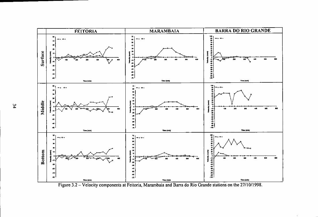
FEITORIA MA RAM BAIA BARRA DO RIO GRANDE
3 C/3
I
.(mki)
•
E o ts o
CO
Tkoafinh)
Figure 3.2 - Velocity components at Feitoria, Marambaia and Barra do Rio Grande stations on the 27/10/1998.
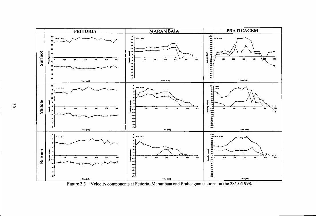
FEITORIA MARAMBAIA PRATICAGEM
C/3
300 400
T>n*(nki)
4;
i
E o
QQ 10a zoo 300
Tkn* tmh)
Figure 3.3 - Velocity components at Feitoria, Marambaia and Praticagem stations on the 28/10/1998.
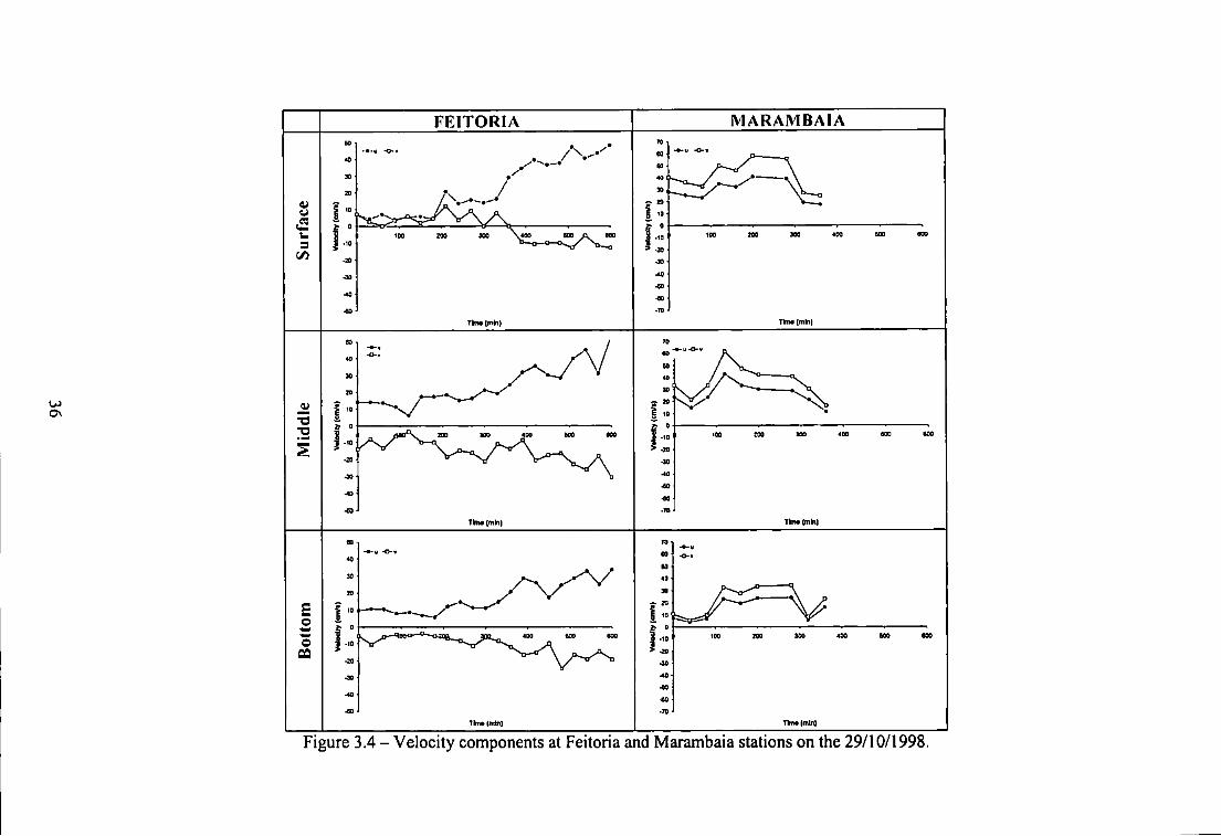
C/)
E o o QQ
FEITORIA
TktM(mh)
IMARAIMBAIA
TkiM(iiih)
TkM(mln)
Figure 3.4 - Velocity components at Feitoria and Marambaia stations on the 29/10/1998.
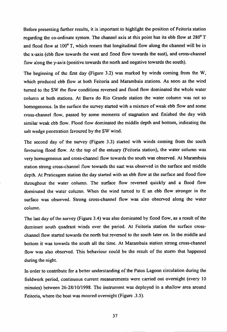
Before presenting further results, it is important to highlight the position of Feitoria station
regarding the co-ordinate system. The chamiel axis at this point has its ebb flow at 280° T
and flood flow at 100° T, which means that longitudinal flow along the channel will be in
the X-axis (ebb flow towards the west and flood flow towards the east), and cross-channel
flow along the y-axis (positive towards the north and negative towards the south).
The beginning of the first day (Figure 3.2) was marked by winds coming fi-om the W,
which produced ebb flow at both Feitoria and Marambaia stations. As soon as the wind
turned to the SW the flow conditions reversed and flood flow dominated the whole water
column at both stations. At Barra do Rio Grande station the water column was not so
homogeneous. In the surface the survey started with a mixture of weak ebb flow and some
cross-channel flow, passed by some moments of stagnation and finished the day with
similar weak ebb flow. Flood flow dominated the middle depth and bottom, indicating the
salt wedge penetration favoured by the SW wind.
The second day of the survey (Figure 3.3) started with winds coming fi-om the south
favouring flood flow. At the top of the estuary (Feitoria station), the water column was
very homogeneous and cross-channel flow towards the south was observed. At Marambaia
station strong cross-channel flow towards the east was observed in the surface and middle
depth. At Praticagem station the day started with an ebb flow at the surface and flood flow
throughout the water column. The surface flow reversed quickly and a flood flow
dominated the water column. When the wind turned to E an ebb flow stronger in the
surface was observed. Strong cross-channel flow was also observed along the water
column.
The last day of the survey (Figure 3.4) was also dominated by flood flow, as a result of the
dominant south quadrant winds over the period. At Feitoria station the surface cross-
chaimel flow started towards the north but reversed to the south later on. In the middle and
bottom it was towards the south all the time. At Marambaia station strong cross-channel
flow was also observed. This behaviour could be the result of the storm that happened
during the night.
In order to contribute for a better understanding of the Patos Lagoon circulation during the
fieldwork period, continuous current measurements were carried out overnight (every 10
minutes) between 26-28/10/1998. The instrument was deployed in a shallow area around
Feitoria, where the boat was moored overnight (Figure .3.5).
37
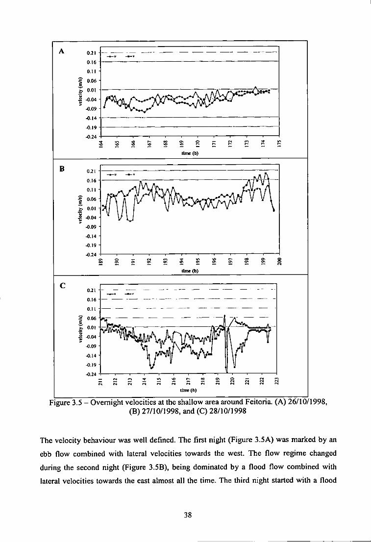
0.21 -
0.16
0.11 -
0.06 •
0.01 -u -0.04 ->
-0.09
-0.14 •
-0.19
-0.24 -
3 llFne(b)
B 0.21 -
0.16 -
C M -
0.06 •
0.01 -
-0.04 • >
-0.09 •
-0.14 -
-0.19 •
-0.24 -
time (h)
0.21 1
^.14 -
time (h)
Figure 3.5 - Overnight velocities at the shallow area around Feitoria. (A) 26/10/1998, (B) 27/10/1998, and (C) 28/10/1998
The velocity behaviour was well defined. The first night (Figure 3,5A) was marked by an
ebb flow combined with lateral velocities towards the west. The flow regime changed
during the second night (Figure 3.53), being dominated by a flood flow combined with
lateral velocities towards the east almost all the time. The third night started with a flood
38
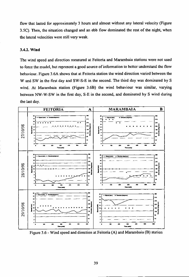
flow that lasted for approximately 3 hours and ahnost without any lateral velocity (Figure
3.5C). Then, the situation changed and an ebb flow dominated the rest of the night, when
the lateral velocities were still very weak.
3.4.2. Wind
The wind speed and direction measured at Feitoria and Marambaia stations were not used
to force the model, but represent a good source of information to better understand the flow
behaviour. Figure 3,6A shows that at Feitoria station the wind direction varied between the
W and SW in the first day and SW-S-E in the second. The third day was dominated by S
wind. At Marambaia station (Figure 3.6B) the wind behaviour was similar, varying
between NW-W-SW in the first day, S-E in the second, and dominated by S wind during
the last day.
F E I T O R I A MARAMBAIA B
C O O n
C O
C O
C O :
Figure 3.6 - Wind speed and direction at Feitoria (A) and Marambaia (B) station
39
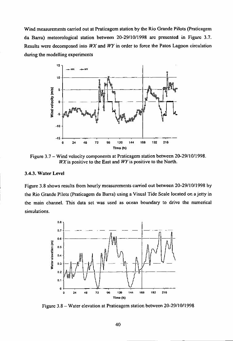
Wind measurements carried out at Praticagem station by the Rio Grande Pilots (Praticagem
da Barra) meteorological station between 20-29/10/1998 are presented in Figure 3.7.
Results were decomposed into IVX and WY in order to force the Patos Lagoon circulation
during the modelling experiments
-15 0 24 48 7 2 96 120 144 168 192 2 1 6
Time (h)
Figure 3.7 - Wind velocity components at Praticagem station between 20-29/10/1998. WX 'is positive to the East and fVYis positive to the North.
3,4.3. Water Level
Figure 3.8 shows results fi^om hourly measurements carried out between 20-29/10/1998 by
the Rio Grande Pilots (Praticagem da Barra) using a Visual Tide Scale located on a jetty in
the main channel. This data set was used as ocean boundary to drive the numerical
simulations.
Figure
TImo (h)
3.8 - Water elevation at Praticagem station between 20-29/10/1998
40
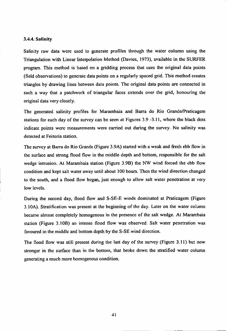
3.4.4. Salinity
Salinity raw data were used to generate profiles through the water column using the
Triangulation with Linear Interpolation Method (Davies, 1973), available in the SURFER
program. This method is based on a gridding process that uses the original data points
(field observations) to generate data points on a regularly spaced grid. This method creates
triangles by drawing lines between data points. The original data points are connected in
such a way that a patchwork of triangular faces extends over the grid, honouring the
original data very closely.
The generated salinity profiles for Marambaia and Barra do Rio Grande/Praticagem
stations for each day of the survey can be seen at Figures 3.9 -3.11, where the black dots
indicate points were measurements were carried out during the survey. No salinity was
detected at Feitoria station.
The survey at Barra do Rio Grande (Figure 3.9A) started with a weak and fi-esh ebb flow in
the surface and strong flood flow in the middle depth and bottom, responsible for the salt
wedge intrusion. At Marambaia station (Figure 3.9B) the NW wind forced the ebb flow
condition and kept salt water away until about 100 hours. Then the wind direction changed
to the south, and a flood flow began, just enough to allow salt water penetration at very
low levels.
During the second day, flood flow and S-SE-E winds dominated at Praficagem (Figure
3.1 OA). Stratification was present at the begirming of the day. Later on the water column
became almost completely homogenous in the presence of the salt wedge. At Marambaia
station (Figure 3.1 OB) an intense flood flow was observed. Salt water penetration was
favoured in the middle and bottom depth by the S-SE wind direction.
The flood flow was still present during the last day of the survey (Figure 3.11) but now
stronger in the surface than in the bottom, that broke down the stratified water column
generating a much more homogenous condifion.
41
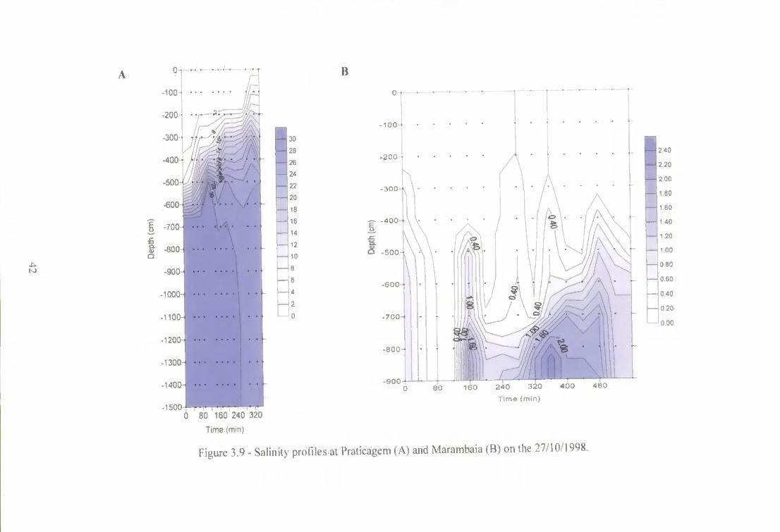
-U
-400 •
- 2 0 0
80 160 240
Time (min)
100 •
400 •
^8
80 160 2 4 0 320 4 0 0
T i m e (min)
2 40
220
2 00
80
6C
4C
20
1 00
0 80
0 60
0 40
0 20
0 00
Figure 3.9 - Salinity profiles at Praticagem (A) and Marambaia (B) on the 27/10/1998.
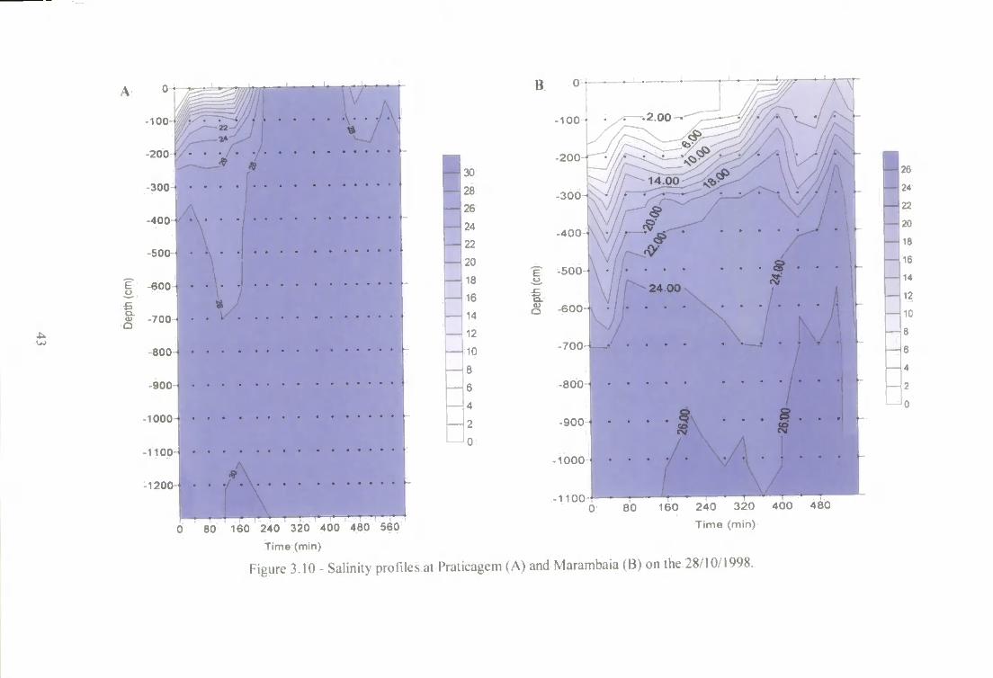
200 *
1000
1100
1200
30
28
26
24
22
20
18
- 16
14
12
10
8
6
4
2
0
-400
24 00
-700
-1000
1100 80 160 240 320 400 480
T ime (min)
26
24
2z
20
18
16
•4
12
10
8
6
4
2
- 0
80 160 240 320 400 480 560 Time (min)
Figure 3.10 - Salinity profiles at Praticagem (A) and Marambaia (B) on the 28/10/1998.
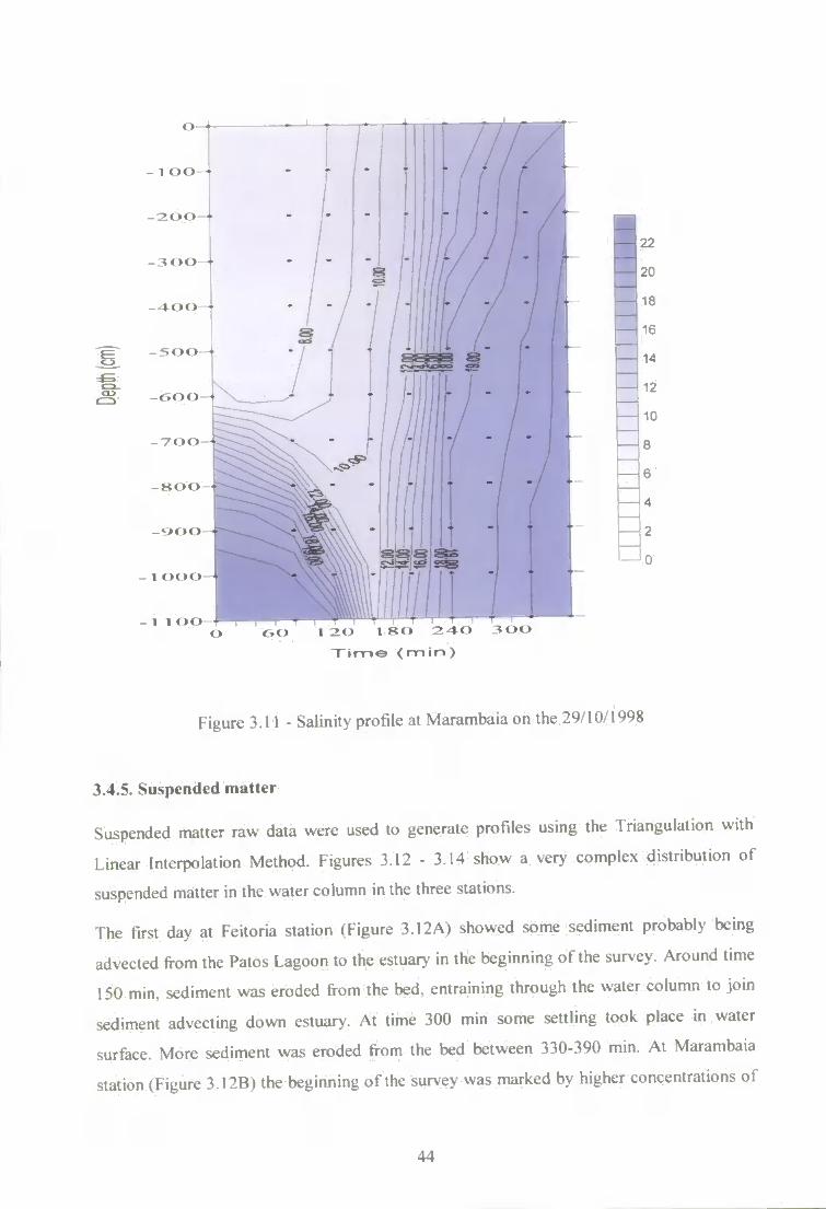
<1>
K M ) •
X i m e ( m i n )
- 7 0 0
I ( > < > < )
1 1<><>
22
20
18
16
14
12
10
8
6
4
2
0
Figure 3.11 - Salinity profile at Marambaia on the 29/10/1998
3.4.5. Suspended matter
Suspended matter raw data were used to generate profiles using the Triangulation with
Linear Interpolation Method. Figures 3.12 - 3.14 show a very complex distribution of
suspended matter in the water column in the three stations.
I hc first day at Feitoria station (Figure 3.12A) showed some sediment probably being
advected from the Patos Lagoon to the estuary in the beginning of the survey. Around time
150 min, sediment was eroded from the bed, entraining through the water column to join
sediment advecting down estuary. At time 300 min some settling took place in water
surface. More sediment was eroded from the bed between 330-390 min. At Marambaia
station (Figure 3.12B) the beginning of the survey was marked by higher concentrations of
44
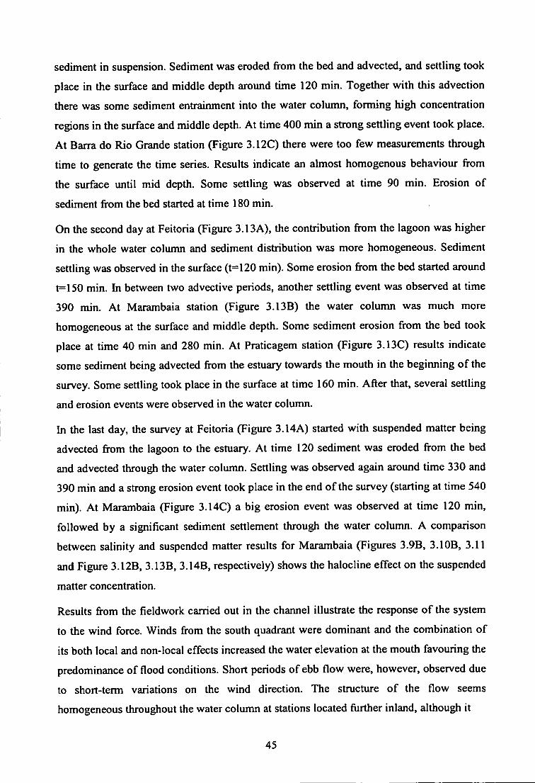
sediment in suspension. Sediment was eroded from the bed and advected, and settling took
place in the surface and middle depth around time 120 min. Together with this advection
there was some sediment entrainment into the water column, forming high concentration
regions in the surface and middle depth. At time 400 min a strong settling event took place.
At Barra do Rio Grande station (Figure 3.12C) there were too few measurements through
time to generate the time series. Results indicate an almost homogenous behaviour from
the surface until mid depth. Some settling was observed at time 90 min. Erosion of
sediment from the bed started at time 180 min.
On the second day at Feitoria (Figure 3.13A), the contribution from the lagoon was higher
in the whole water column and sediment distribution was more homogeneous. Sediment
settling was observed in the surface (t=120 min). Some erosion from the bed started around
t=150 min. In between two advective periods, another settling event was observed at time
390 min. At Marambaia station (Figure 3.13B) the water column was much more
homogeneous at the siu-face and middle depth. Some sediment erosion from the bed took
place at time 40 min and 280 min. At Praticagem station (Figure 3.13C) results indicate
some sediment being advected from the estuary towards the mouth in the beginning of the
survey. Some settling took place in the surface at time 160 min. After that, several settling
and erosion events were observed in the water column.
In the last day, the survey at Feitoria (Figure 3.14A) started with suspended matter being
advected from the lagoon to the estuary. At time 120 sediment was eroded from the bed
and advected through the water column. Settling was observed again around time 330 and
390 min and a strong erosion event took place in the end of the survey (starting at time 540
min). At Marambaia (Figure 3.14C) a big erosion event was observed at time 120 min,
followed by a significant sediment settlement through the water column. A comparison
between salinity and suspended matter results for Marambaia (Figures 3.9B, 3.10B, 3.11
and Figure 3.12B, 3,13B, 3.14B, respectively) shows the halocline effect on the suspended
matter concentration.
Results from the fieldwork carried out in the channel illustrate the response of the system
to the wind force. Winds from the south quadrant were dominant and the combination of
its both local and non-local effects increased the water elevation at the mouth favouring the
predominance of flood conditions. Short periods of ebb flow were, however, observed due
to short-term variations on the wind direction. The structure of the flow seems
homogeneous throughout the water column at stations located fiarther inland, although it
45
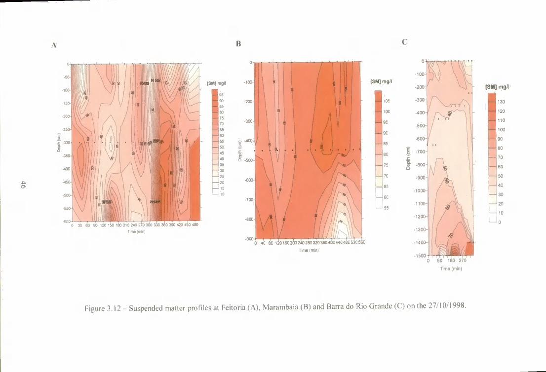
W 120 150 ieO 210 240 270 300 330 T)(T«(n«n)
[SM] mg/l
90
86
80
75
'0
65
4.
35
3C.
25 I—120 — 15 — 10
[SM] mg/l
105
I X
9f
9C
85
0 4C 8C l2Cl6C20C24C28C32C36C4a44C48C52C56C
Time (mm)
-300 •
-lOOO-J
1100H
1200 •!
•1500
[SM] mg/l
130
120
110
100
90
80
70
60
50
4-:
30
20
1G
0
0 90 180 270
Time (mm)
Figure 3.12 - Suspended matter profiles at Feitoria (A). Marambaia (B) and Barra do Rio Grande (C) on the 27/10/1998.
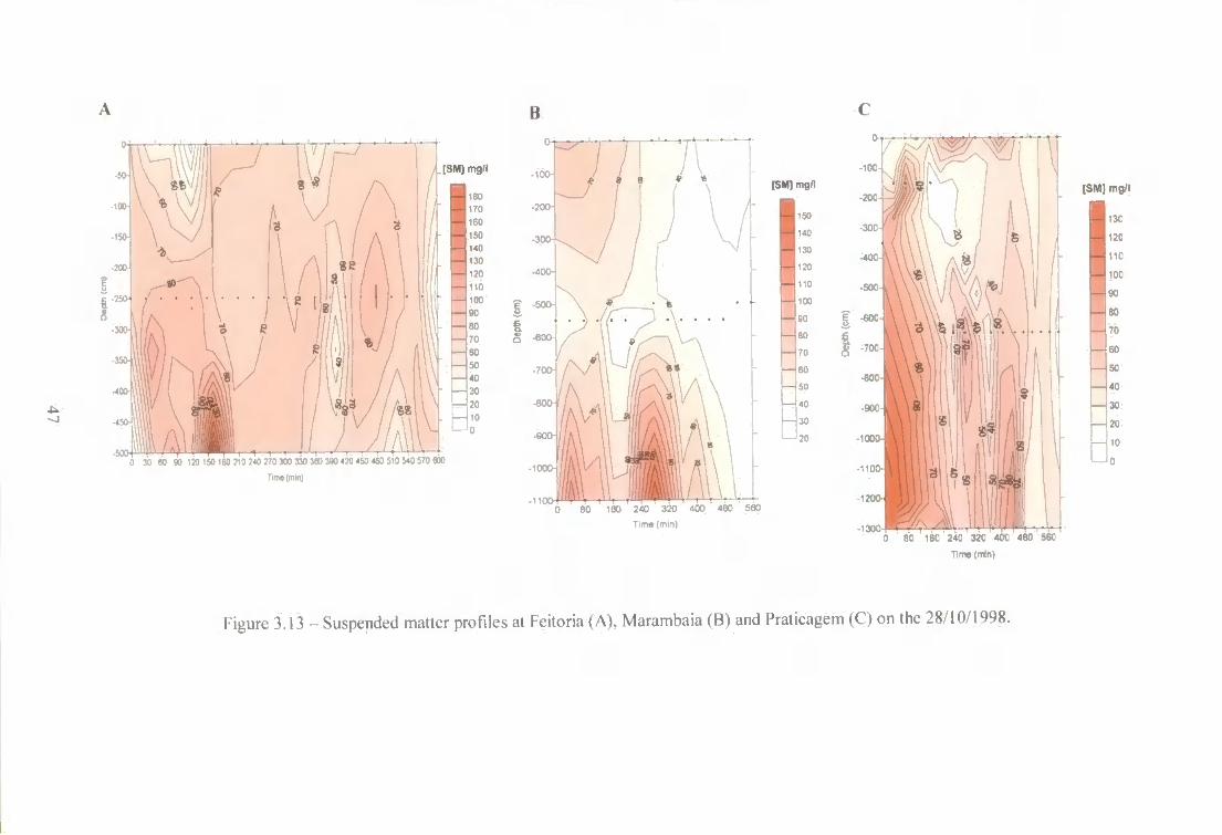
n
- J
' [SM] mg/l
0 30 80 90 120 150 180 210 240 270 300 330 3 « 380 420 450 480 510 540 570 800
Tim« (mm)
80 100 240 320 400 Tim« (mm)
480 580 I M l
[SM] mg/l
13C
12C
11C
IOC
190
8C
70
60
50
-40
3C
2C
10
0
8C 18C 24C 32C 40C 480 56C Time (min)
Figure 3.13 - Suspended matter profiles at Feitoria (A), Marambaia (B) and Praticagem (C) on the 28/10/1998.
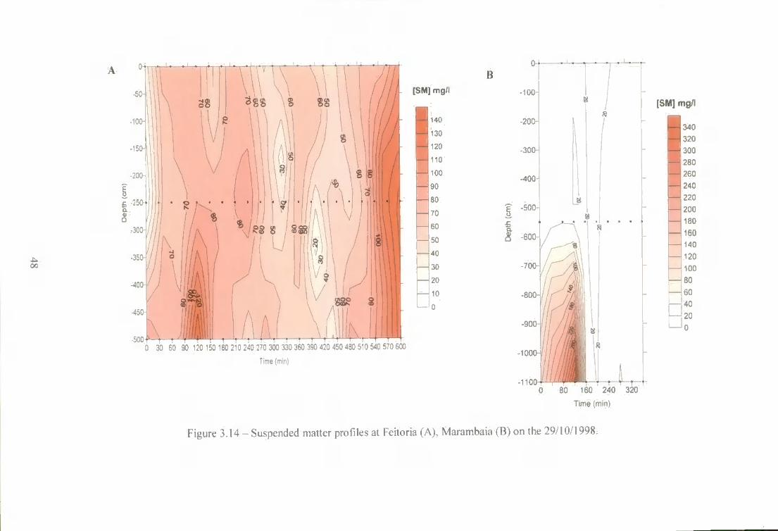
[SM] mg/l
I'. * * •
A
n
0 30 60 90 120 150 180 210 240 270 300 330 360 390 420 450 480 510 540 570 600
Time (mm)
,5 -600
-1000
-1100
[SM] mg/l
340
- 320
- 300
- 280 260
- 240
- 220 200 180 160 140 120 100 80
- 60 4C 20
— 0
0 80 160 240 320
Time (min)
Figure 3.14 - Suspended matter profiles at Feitoria (A), Marambaia (B) on the 29/10/1998,
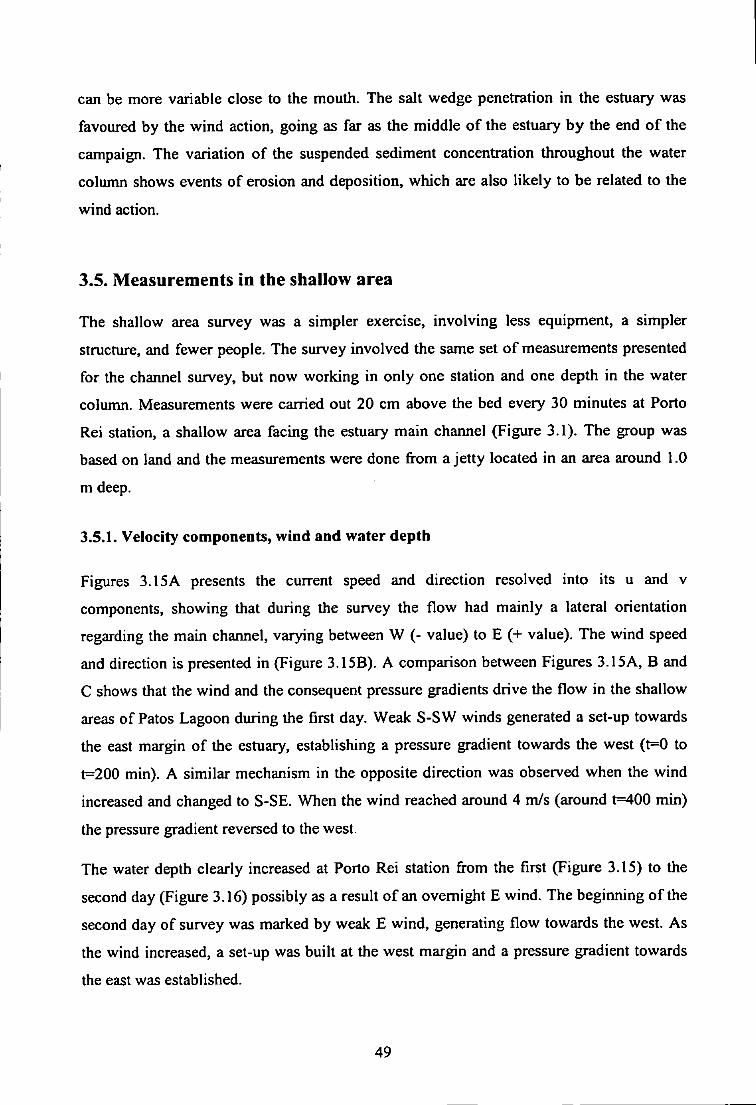
can be more variable close to the mouth. The salt wedge penetration in the estuary was
favoured by the wind action, going as far as the middle of the estuary by the end of the
campaign. The variation o f the suspended sediment concentration throughout the water
column shows events of erosion and deposition, which are also likely to be related to the
wind action.
3.5. Measurements in the shallow area
The shallow area survey was a simpler exercise, involving less equipment, a simpler
structure, and fewer people. The survey involved the same set of measurements presented
for the channel survey, but now working in only one station and one depth in the water
column. Measurements were carried out 20 cm above the bed every 30 minutes at Porto
Rei station, a shallow area facing the estuary main channel (Figure 3.1). The group was
based on land and the measurements were done from a jetty located in an area around 1.0
m deep.
3.5.1. Velocity components, wind and water depth
Figures 3.15A presents the current speed and direction resolved into its u and v
components, showing that during the survey the flow had mainly a lateral orientation
regarding the main channel, varying between W (- value) to E (+ value). The wind speed
and direction is presented in (Figure 3.15B). A comparison between Figures 3.15A, B and
C shows that the wind and the consequent pressure gradients drive the flow in the shallow
areas of Patos Lagoon during the first day. Weak S-SW winds generated a set-up towards
the east margin of the estuary, establishing a pressure gradient towards the west (t=0 to
t=200 min). A similar mechanism in the opposite direction was observed when the wind
increased and changed to S-SE. When the wind reached around 4 m/s (around t=400 min)
the pressure gradient reversed to the west.
The water depth clearly increased at Porto Rei station from the first (Figure 3.15) to the
second day (Figure 3.16) possibly as a result of an overnight E wind. The beginning of the
second day of survey was marked by weak E wind, generating flow towards the west. As
the wind increased, a set-up was built at the west margin and a pressure gradient towards
the east was established.
49
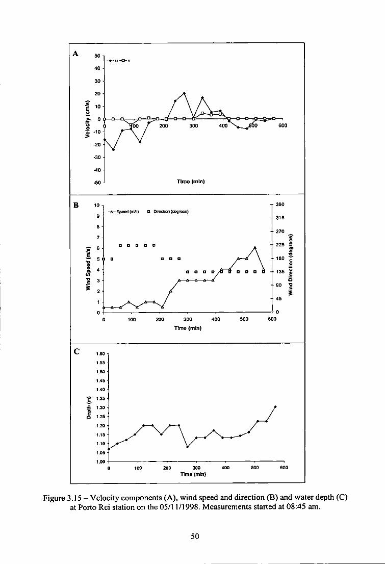
600
Time (mln)
B Spood(m/!5) O OirecBon (degrees}
225 e
100 200 300
Time (mln)
400 500 600
1,60 1
1.55
1.50
1.45
1.40
1.35
1.30
1.25
1.20
1.15
1.10
1.05 H
1.00
Time (mm) 600
Figure 3.15 - Velocity components (A), wind speed and direction (B) and water depth (C) at Porto Rei station on the 05/11/1998. Measurements started at 08:45 am.
50
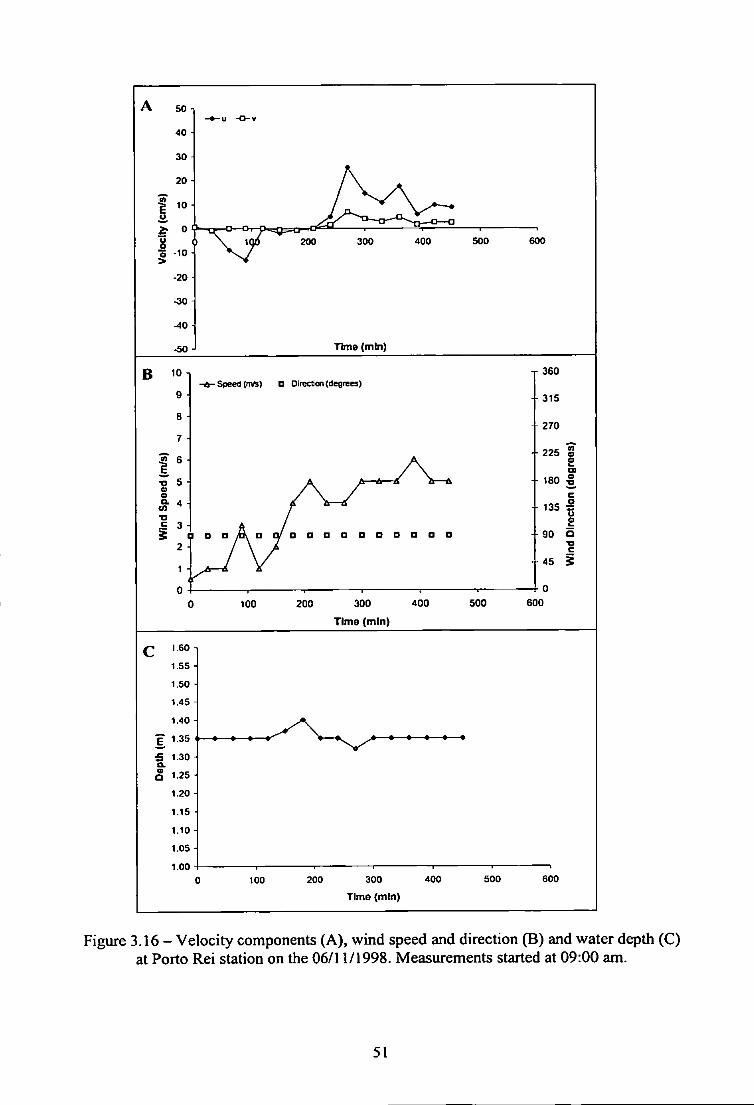
50
40
30
20
t 0
I -10 i
-20
-30
-40
-50
200 300 400 500 600
TJmo (min)
speed (mfS) • Direction (degrees)
+ 180 ^
SO a
300
Time (mIn)
1.60 n
1.55
1.50
1.45
1.40
B 1.25
1.20
1.15
1.10
1.05
1.00
S 1.30
100 200 300
Time (min)
400 500 600
Figure 3.16 - Velocity components (A), wind speed and direction (B) and water depth (C) at Porto Rei station on the 06/11/1998. Measurements started at 09:00 am.
51
3.5.2. Salinity and suspended matter
Figure 3.17 describes the behaviour of salinity and suspended matter at Porto Rei station.
During the first day of the survey (Figure 3.17A), salinity levels were low and did not vary
significantly with time. The suspended particulate matter concentration had a very well
defined behaviour with peaks of high concentration at t=60 min, between t=160 - 240 min,
and between 480 - 570 min. These peaks are likely to be related to erosion events due to
the wind or to advection o f suspended matter fix)m other areas. In the second day (Figure
3.17B), suspended matter concentrations were lower, probably as the result of flocculation
induced by the salinity higher levels.
100
90
80
70 +
% 60
§ 50
£2. 40
30
20
10
l[SPM) (mg/1) Salinity t35
i 3 0
25
20 £.
15 «
10
W5
^ s s § S g g I g § g § g § S 2 S S in uS Eo Time (mtn)
B 100
90
80 -
70
|[SPM] (mg/l) Sannity 35
30
+ 25
20 >.
15 W " 40
Tbne (min)
Figure 3.17 - Salinity and suspended matter concentration at Porto Rei station. (A) 05/11/1998 and (B) 06/11/1998.
52
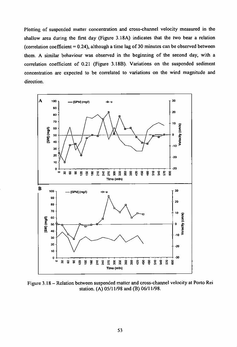
Plotting of suspended matter concentration and cross-channel velocity measured in the
shallow area during the first day (Figure 3.18A) indicates that the two bear a relation
(correlation coefficient = 0.24), although a time lag of 30 minutes can be observed between
them. A similar behaviour was observed in the beginning of the second day, with a
correlation coefficient of 0.21 (Figure 3.1 SB). Variations on the suspended sediment
concentration are expected to be correlated to variations on the wind magnitude and
direction.
— SPM](mg/l)
Time (mln)
B — (SPMKmgfl)
o s s 8 § S g 5 I g § § g I f S § - ? ° m A in
Tbne (mfri)
Figure 3.18- Relation between suspended matter and cross-channel velocity at Porto Rei station. (A) 05/11/98 and (B) 06/11/98.
53
By the end of the whole fieldwork it was clear that measurements and the overall fieldwork
experience are essential towards an understanding of the system. However, a detailed
hydrodynamic study cannot be completely carried out based on field data alone because of
the large spatial and temporal variability. Such a study would require a large number of
field observations, and the costs associated with data collection are usually quite high. A
possible solution to paucity of field data is the use of numerical models as sophisticated
techniques for interpolation and extrapolation of field data in both spatial and temporal
domains. Such predictions can provide detailed information about the response of the
system to different forcing effects, as well as an idea of the overall circulation pattern
through time.
Conversely, it is equally important to recognise that meaningful and realistic modelling
results cannot be obtained without adequate supporting data for model calibration and
validation (Cheng et ai, 1991). Thus, field data collection and numerical modelling must
be considered as two inseparable and complementary elements of one integrated research
programme.
54
Chapter 4
Description of the model
4.1. Introduction
The study of fluid motion in rivers, lakes and estuaries is of great importance in the
understanding of many environmental problems, because many transport phenomena are
strongly dependent on a proper description o f the hydrodynamic processes (Cheng &
Walters, 1982). The solution of the appropriate governing system of equations has, often
been used as a means to enhance further understanding of the physical processes. When the
realistic situation is too complex, a modelled system that encompasses the essential
features of the problem is necessary (Cheng, 1978).
The governing equations of fluid flow are the Navier-Stokes equations, which can be
solved by two basic types of numerical model. One is based on finite differences, and the
other is based on finite elements (Dyke, 1996). In the past, the numerical solution o f these
equations has mainly been achieved by the finite difference technique, where the resulting
flow patterns have been shown to correspond, within acceptable tolerances, to
experimental results (Cheng, 1970). When the governing equations are known, but
complicated geometry or boundary conditions render analytical solutions difficult or
impossible to obtain, the finite element method is often employed (Brookes & Hughes,
1982). In recent years, the finite element method has become increasingly popular in
almost every engineering field. For a direct comparison of various finite-element shapes
versus various degrees of finite difference approximations see Gray & Pinder (1976).
The finite element method was initially developed by researchers in the aircraft industry as
an effective means for solving aeroelasticity problems (Argyris & Kelsey, 1960; Turner et
al., 1956). Oceanographic studies employing the Finite Element Method (FEM) have been
published since the early 1970s. From the start, the primary attraction of the FEM has been
the rigorous mathematical approach to problems with strong spatial inhomogeneity, arising
either from topography (banks, coast) or from steep internal gradients in the flow (fronts,
jets). The use of unstructured, nonuniform computational grids of variably sized triangular
elements allows, in principle, high resolution o f such local features without necessarily
sacrificing the horizontal extent of the model (Lynch et al., 1996).
55
Following two decades o f intensive development and application to the general ocean
circulation (Fix, 1975; Haidvogel et aL, 1980; Le Provost, 1986; Ma, 1993; Iskandarani et
aL, 1995; Le Provost et aL, 1994), to the shelf break (Werner, 1987), to oceanic tides
(Platzman, 1978; Le Provost & Vincent, 1986; Vincent & Le Provost, 1988; Le Provost et
aL, 1995) and to continental shelf studies (Lynch & Werner, 1991a; Lynch et aL, 1992;
Naimie et aL, 1994), the benefits of the FEM for oceanographic applications are now
firmly established and workable algorithms are available (Lynch et aL, 1996). Studies of
estuarine and shelf circulation appeared as early as 1973 (Grotkop, 1973; Wang &
Connor, 1975), and have developed in the last two decades (Walters, 1992; Greenberg et
aL. 1997).
Lynch et aL (1996) comment about additional recent field-scale FEM studies that have
been carried out in the Gulf o f Venezuela/Lake Maracaibo (Lynch et aL, 1990); the
Alboram Sea (Lynch et aL, 1989); the Gulf of Maine (Lynch et aL, 1992); the Bight of
Abaco (Westerink et aL, 1989); the south-west coast o f Vancouver Island (Foreman &
Walters, 1990; Foreman et aL, 1992a, b; Walters & Foreman, 1992); the south Atlantic
Bight (Werner et aL, 1993); the Delaware Bay (Walters, 1992); and the Gulf of Mexico
(Westerink et aL, 1992; Blain et aL, 1994). Several of these studies are active today and
have been extended to include three-dimensional computations based on conventional
velocity (Lynch & Werner, 199lb) and novel "direct stress" approaches (Luettich &
Westerink, 1991; Luettich et aL, 1994); studies of convergence of solutions based on mesh
discretization (Westerink et aL. 1994; Luettich & Westerink, 1995; Lynch et aL. 1995);
radiation boundary conditions (Johnsen & Lynch, 1994, 1995); and computations on
special coordinate systems (Kolar et aL ,1994).
4.2. The T E L E M A C System
The TELEMAC system was developed by the Laboratoire National d'Hydraulique (LNH),
part of the Studies and Research Division (DER) of Electricite de France (EDF).
TELEMAC is a flow model based on the finite element technique developed to simulate
the flow in rivers, estuaries and coastal waters. The system is modular, and the calculated
hydrodynamics can be used in other modules of the system in order to deal with water
quality, sediment transport, and also for coupling with wave models (Figure 4.1).
56
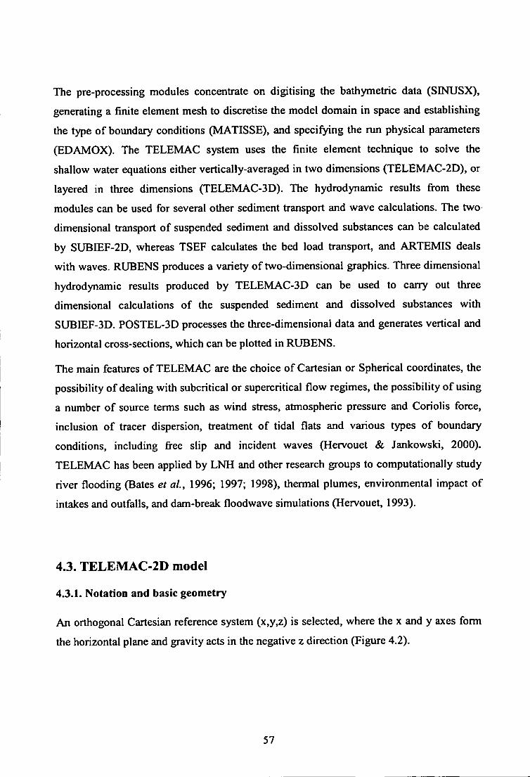
The pre-processing modules concentrate on digitising the bathymetric data (SINUSX),
generating a finite element mesh to discretise the model domain in space and establishing
the type of boundary conditions (MATISSE), and specifying the run physical parameters
(EDAMOX). The TELEMAC system uses the finite element technique to solve the
shallow water equations either vertically-averaged in two dimensions (TELEMAC-2D), or
layered in three dimensions (TELEMAC-3D). The hydrodynamic results from these
modules can be used for several other sediment transport and wave calculations. The two
dimensional transport of suspended sediment and dissolved substances can be calculated
by SUBIEF-2D, whereas TSEF calculates the bed load transport, and ARTEMIS deals
with waves. RUBENS produces a variety of two-dimensional graphics. Three dimensional
hydrodynamic results produced by TELEMAC-3D can be used to carry out three
dimensional calculations of the suspended sediment and dissolved substances with
SUBIEF-3D. P0STEL-3D processes the three-dimensional data and generates vertical and
horizontal cross-sections, which can be plotted in RUBENS.
The main features of TELEMAC are the choice of Cartesian or Spherical coordinates, the
possibility of dealing with subcritical or supercritical flow regimes, the possibility of using
a number of source terms such as wind stress, atmospheric pressure and Coriolis force,
inclusion of tracer dispersion, treatment of tidal flats and various types of boundary
conditions, including free slip and incident waves (Hervouet & Jankowski, 2000).
TELEMAC has been applied by LNH and other research groups to computationally study
river flooding (Bates et al, 1996; 1997; 1998), thermal plumes, environmental impact of
intakes and outfalls, and dam-break floodwave simulations (Hervouet, 1993).
4.3. TELE1VIAC-2D model
4.3.1. Notation and basic geometry
An orthogonal Cartesian reference system (x,y,z) is selected, where the x and y axes form
the horizontal plane and gravity acts in the negative z direction (Figure 4.2).
57
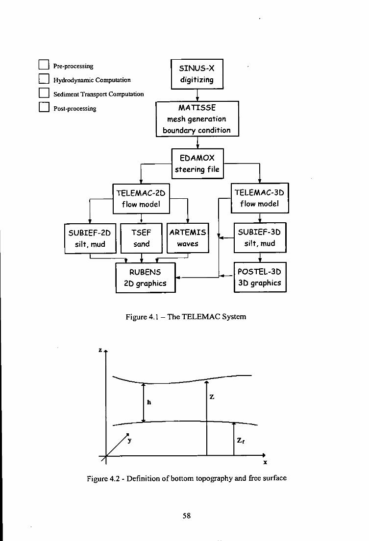
• Pre-processing • Hydrodynamic Computation
Sediment Transport Computation
I Post-processing
S I N U S - X digitizing
M A T I S S E mesh generation
boundary condition
EDAAAOX steering file
TELEMAC-2C> flow model
SUBIEF-2D silt, mud
T S E F sand
ARTEMIS waves
RUBENS 2D graphics
TELEMAC-3D flow model
SUBIEF-3D silt, mud
— ] — POSTEL-3D BO graphics
Figure 4.1 - The TELEMAC System
7
Figure 4.2 - Definition of bottom topography and fi-ee surface
58
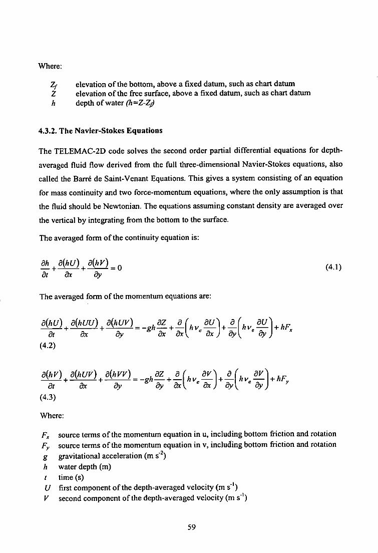
Where:
Z/ elevafion o f the bottom, above a fixed datum, such as chart datum Z elevation of the fi^ee surface, above a fixed datum, such as chart datum h depth of water (h =Z-Zj)
4.3.2. The Navier-Stokes Equations
The TELEMAC-2D code solves the second order partial differential equafions for depth-
averaged fluid flow derived from the ftill three-dimensional Navier-Stokes equations, also
called the Barr6 de Saint-Venant Equations. This gives a system consisting of an equation
for mass continuity and two force-momentum equations, where the only assumption is that
the fluid should be Newtonian. The equations assiiming constant density are averaged over
the vertical by integrating fi^om the bottom to the surface.
The averaged form of the continuity equation is:
^ + « + « = 0 (4.1) dt dx dy
The averaged form of the momentum equations are:
d{hU) ^ djhUU) ^ djhUV)^ gh^^ \ ^ dt dx dy dx dx
(4.2) I, dx)
d + —
dy
hv dU
d{hV) ^ djhUV) ^ djhW)^ ^^dZ ^ d L A dt dx dy dy dx\ ^ dx) dy
(4.3)
Where:
Fx source terms o f the momentum equation in u, including bottom fiiction and rotation Fy source terms of the momentum equation in v, including bottom fiiction and rotation g gravitational acceleration (m s' ) h water depth (m) / time (s) V first component of the depth-averaged velocity (m s"*) V second component of the depth-averaged velocity (m s"')
59
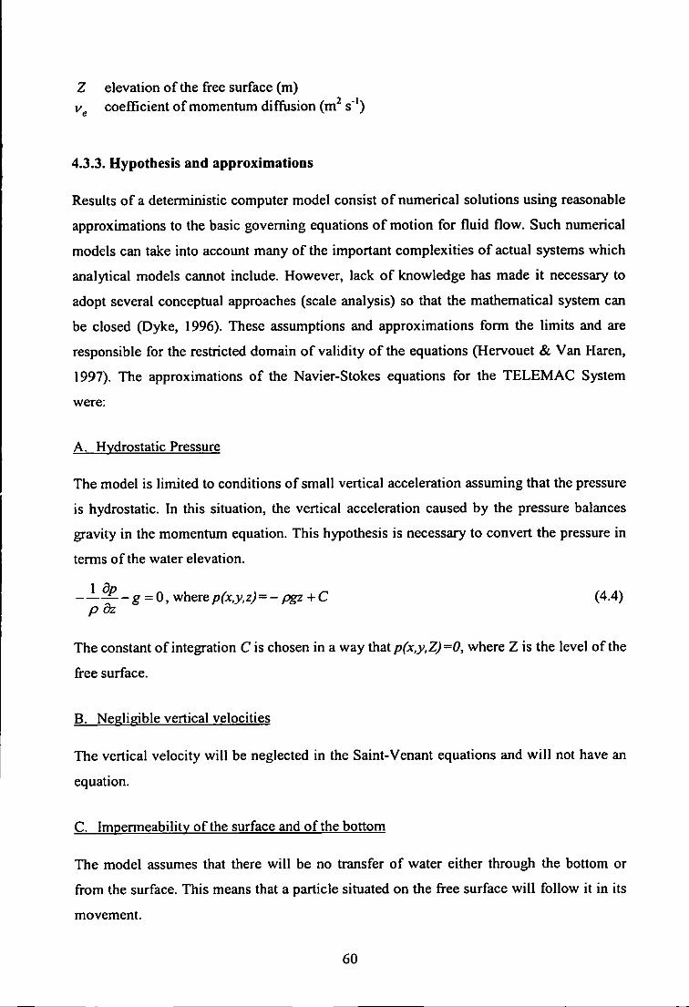
Z elevation of the free surface (m) V coefficient of momentum diffusion (m^ s"*)
4.3.3. Hypothesis and approximations
Results of a deterministic computer model consist of numerical solutions using reasonable
approximations to the basic governing equations o f motion for fluid flow. Such numerical
models can take into account many of the important complexities of actual systems which
analytical models cannot include. However, lack of knowledge has made it necessary to
adopt several conceptual approaches (scale analysis) so that the mathematical system can
be closed (Dyke, 1996). These assumptions and approximations form the limits and are
responsible for the restricted domain o f validity o f the equations (Hervouet & Van Haren,
1997), The approximations of the Navier-Stokes equations for the TELEMAC System
were:
A. Hydrostatic Pressure
The model is limited to conditions of small vertical acceleration assuming that the pressure
is hydrostatic. In this situation, the vertical acceleration caused by the pressure balances
gravity in the momentum equation. This hypothesis is necessary to convert the pressure in
terms of the water elevation.
- — ^ - ^ = 0, where p(x,y.z) =-pgz-^C (4.4) p oz
The constant of integration C is chosen in a way that p(x,y,Z)=0, where Z is the level of the
free surface.
B. Negligible vertical velocities
The vertical velocity wi l l be neglected in the Saint-Venant equations and w i l l not have an
equation.
C. Impermeability of the surface and of the bottom
The model assumes that there wi l l be no transfer of water either through the bottom or
from the surface. This means that a particle situated on the free surface wi l l follow it in its
movement.
60

^ - ^ ^ • - 0 (4.5)
^ + C7^.^ = 0 (4.6)
Where:
I j f velocity at the bottom 17 velocity at the free surface n vector normal to the surfaces 2f elevation of the bottom Z elevation of the free surface
4.3.4. Source terms of the momentum equations
A. Friction at the bottom
In TELEMAC-2D the bed friction is represented as a quadratic function of velocity:
T=pCf\V\V (4.7)
Where:
P density of the water (kg m"'') Cf friction coefficient (dimensionless) ( ] depth-averaged velocity of the flow (m s'*)
The friction coefficient (C/) can be parameterised either in terms of the Chezy (C in m*'
s*'). Manning {m, in m^'^ s ' ) , or Nikuradse {Ks in mm) friction coefficients. The Chezy
formulas for the friction force at the bottom to be added to the momentum equation
become:
l ^ ^ W w U v ^ (4.8) cos(a) hC^
^ cos(a)/iC^
Where:
Fx source terms of the momentum equation in u Fy source terms of the momentum equation in v
61

g gravitational acceleration h water depth u velocity first component V velocity second component a slope angle of the bottom
^ Chezy fiiction coefficient(Cj- = g/C )
When the Manning law of bottom fiiction is applied, the fiiction coefficient is substituted
by:
C f = ^ (4.10)
When the Nikuradse law of bottom friction is chosen the friction coefficient is substituted
by:
C, J 5- (4.11) 14.8A 1
32^101
Where:
Q fiiction coefficient (dimensionless) m Manning fiiction coefficient Ks Nikuradse fiiction coefficient g gravitational acceleration h water depth
B. Coriolis Acceleration
The Coriolis force at a point of latitude ^ is equal to:
= 2o}vs\n(p = Jv (4.12)
Fy =-Ionising = -/u (4.13)
Where:
Fx source terms of the momentum equation in u Fy source terms o f the momentum equation in v 0) angular velocity of the Earth's rotation = 7.292 x 10' rad s * / Coriolis coefficient (negative in the Southern Hemisphere)
62
C. Wind effect
Analogous to the analysis of fiiction at the bottom, the resistance o f the wind takes the
following form:
Fy ^ \^a^,^,V^,,,4ul„,^Vl,„, (4.15) h p
Where:
Fx source terms of the momentum equation in u Fy source terms of the momentum equation in v P density of fi-eshwater (1000 kg m"^)
Pair density of the air (1.023 kg m'^) Owind wind resistance coefficient
Uy,ind, Vwind components of the wind velocity
The value of Ah-iW can be obtained from many different formulas. The TELEMAC System
uses the formula proposed by the Institute of Oceanographic Sciences (UK):
I f U wind <5 ms"', a^,-„. =0.565x10 ^
I f 5 < ^wind < 19,22 ms\a^,.„, =(-OA2-^0A3l\u^^)x
I f ^wind > 19,22 m s ", a^i„^ =2.513x10 -3
4.3.5. Boundary Conditions
For the solid boundaries TELEMAC considers that:
• no mass flux of water occurs through the bottom and closed lateral faces (i7 •« = O),
where n is the unit normal vector of the boundary;
63
• there is a free slip condition at the wall for all vectors tangent to the wall
dn
the friction condition at the bed is written as
friction coefficient provided by the user.
on y where a is the
• the water surface height is free and the surface boundary condition is a stress calculated
from the wind speed and coefficient o f wind influence.
For the open liquid boundaries the user can define, for each of the principal variables {h, U,
V), i f there is a prescribed or free value in each point of the mesh. Based on that, two
situations were chosen for the present study: 1) prescribed flowrate and free elevation at
the top of the lagoon; 2) free velocity and prescribed elevation at the mouth.
4.3.6. Turbulence modelling
TELEMAC-2D solves equations ( I ) , (2), and (3) for the three unknowns A, U, and V. The
model employs a mean flow concept to treat turbulent flows, averaging instantaneous
velocities over time to give mean motion only (Reynolds averaging). In this fomiulation,
an additional term, the Reynolds stress, is added to the governing equations to represent the
increased internal shear stress on mean flow produced by velocity fluctuations (Hervouet
& V a n Haren, 1996).
The system o f equations obtained is not soluble because it is not closed. This difficulty has
therefore given rise to turbulence models called Closure Models. There are two ways to
obtain a closure of the Reynolds equations. The first and more elaborate method consists of
developing explicit equations for the Reynolds stress tensor (Hervouet & Van Haren,
1996). Most turbulence models, however, apply the Boussinesq eddy-viscosity concept
(not to be conftised with the Boussinesq approximation) (Hervouet & Van Haren, 1996;
Bates et al, 1997), which expresses the Reynolds stress tensor in terms of the local
velocity gradient and introduces a turbulent viscosity.
TELEMAC-2D applies the Boussinesq eddy-viscosity concept and offers the possibility of
using a constant viscosity or o f solving directly the transport equations for the kinetic
64
energy and its rate of dissipation, which constitutes the k-e model. Constant viscosity was
assumed for simulations presented here.
4.3.7. Tidal Flats
Many of the recent studies performed with TELEMAC involve wetting and drying areas.
This seems increasingly common and is linked to the increasing number o f environmental
problems resorting to hydraulics in rivers or estuaries. The ability to cope with such
situations is thus of utmost importance. The problem is the behaviour o f the numerical
algorithms in the dry zones, e.g. some terms in the equations have h in the denominator
and they therefore tend to infinity as h tends to zero (Hervouet & Van Haren, 1996).
TELEMAC-2D offers two radically different options for treating tidal flats (Hervouet &
Janin, 1994; Hervouet & Van Haren, 1996). The first consists of treating them integrally
and in the entire domain, by correcting the gradient of the fi'ee surface. The second option
consists o f removing fi-om the calculation all the elements that are not entirely wet.
Hervouet & Van Haren (1996) recommend that in cases with very steep slopes, removing
the dry elements is better, and when there is a very small number of elements in a cross-
section, solving the equations everywhere is preferable.
When applying the correction of gradient of the fi-ee surface, initially a check is made for
each element to test for the existence o f a partially dry element. I f the bed elevation for a
particular node (Z/^) with depth //^ is greater than the water surface elevation (2/7+///) at
one of the other nodes in that element, then a new water surface elevation (zp) for the dry
node is defined in the momentum equation {zz-Z/i-^hz). Moreover, as only the momentum
equation is modified, mass conservation properties are not affected (Bates et al, 1997).
This solution is comparatively simple when compared to other approaches to this problem
(Lynch & Gray, 1980; Kawahara & Umetsu, 1986; Leclerc et al, 1990), and is
computationally efficient, introducing no additional unknowns into the equations (Bates et
al, 1998).
In three-dimensional computations, an additional difficulty is the fact that the volume of
elements is zero when there is no water. Thus, only the removal of dry elements is
practicable (Hervouet & Van Haren, 1996).
65
4.3.8. Numerical methods
The Navier-Stokes equations are solved based on the Operator-Splitting method (Marchuk,
1975; Zienkiewicz & Ortiz, 1995), whose main principle is that the hyperbolic and
parabolic parts of the Navier-Stokes equations should be treated separately in order to use
well-adapted numerical methods for each part. The solution involves two steps: 1) solution
of the advection terms; 2) solution of the propagation, difRision and source terms.
A. Advection Step
The Method o f Characteristics is applied to solve the advection o f u and v (Galland et al.,
1991; Bates et ai. 1997; 1998). In TELEMAC-2D the calculation of the characteristics
(trajectories) are performed by a method of Runge-Kutta of order 1, and the interpolation
at the foot of the characteristic conforms to the type of finite element chosen for the
"propagation-diffusion-source terms"stage. Runge-Kutta method o f order 2 has been tested
but does not provide any significant improvement and it is also more expensive.
The Streamline Upwind Petrov-Galerkin method (SUPG) has been applied to solve the
advection of h (Brookes 8c Hughes, 1982). This method was implemented in TELEMAC-
2D to ensure mass conservation and an oscillation fi-ee solution without excessive mesh
refinement, or the addition o f artificial diffiisivity (Bates et aL, 1998). Extended to a
Petrov-Galerkin formulation, the standard Galerkin weighting ftmctions are modified by
adding a streamline upwind perturbation. The modified weighting fiinction is applied to all
terms in the equation, resulting in a consistent weighted residual formulation.
B. Propagation, diffusion and source terms step
The propagation, diffusion and source terms are solved by the finite element method,
where an implicit time discretisation allows the calculation of the non-linearities in the
equations. Variational formulations and space discretisation transform the continuous
equations into a linear discrete system where the values of u and v at the nodes are the
unknown variables. This system is solved by an iterative conjugate gradient method
(Hervouet and Van Haren, 1994). TELEMAC-2D makes significant savings in both
computational time and storage requirements through the use o f an element-by-element
66
solution technique, where the matrices in the linear system are stored in their elementary
form without recourse to ful l assembly (Bates et al., 1997).
4.4. TELEMAC-3D model
TELEMAC-3D solves the three-dimensional Navier-Stokes equations for free surface
flows accepting the hypothesis of hydrostatic pressure. This approximation means that the
resulting equations are only suitable to calculate typical shallow water applications in
which the vertical velocities are much smaller than the horizontal ones. However, they are
very useful because they provide information about the structure o f the flow in the vertical
and also make it possible to take into account vertical density fluctuations (Hervouet &
Van Haren, 1996).
Several features are broadly the same in TELEMAC-2D and TELEMAC-3D; thus special
attention wi l l be given only to the specific features arising in TELEMAC-3D.
A. Hvdrostatic pressure approximation:
In order to derive the hydrostatic pressure approximation, pressure and density are
decomposed into mean values po(z) and Po(z), and fluctuations around these mean values,
4P and Ap, as follows:
p(z)=/7o(z) + ( z ) (4.16)
p{z)=Po{z)-^Ap{z) (4.17)
Supposing that the mean flow structure is in a state of hydrodynamic equilibrium, so that:
dz
and that the variations around the equilibrium state are negligible (Ap/po « 1 and Ap/po
« 1 ) , the decompositions can eventually be substituted into the momentum equations. That
is called the Boussinesq approximation of the Navier-Stokes equations.
67
However, as far as the shallow water equations are concerned, the vertical momentum
equation is used only to derive an expression for the pressure fluctuations, due to density
fluctuations. Supposing that vertical velocities are sufficiently small, and neglecting
diffusion and source terms, then only the pressure and gravity terms remain in the vertical
momentum equation:
p dz PQ (4.19)
The fluctuating part of the pressure can then be found to have the following part (where the
density po(z) is replaced by a reference density, denoted by p :
(4.20)
B. TELEMAC-3D equations
The final set of equations used in TELEMAC-3D are then the continuity (Eq. 4.21),
momentum equations (Eqs. 4.22, 4.23, 4.24), tracer (Eq. 4.25) and equation of state (Eq.
4.26):
dh ^ djhu) ^ a(/,v) ^ djhw) Q dt dx dy dz
dii du du du \ dp d ( dit^ + M + V + W = - — - £ - + —
dt dx dy dz p dx dx\ dx J dy du^
dz ' diA
(4.21)
(4.22)
dv dv dv dv \ dp d ( dv^ d — + M — + v — + w — = - — — + — dt dx dy dz p dy dx
dv dzK'dz)
PQ
(4.23)
(4.24)
dT dT dT dT d — + w — + V + i V — = — dt dx dy dz dx
^ 1 I + — \ " ^ 1 ^ dz J + Q (4.25)
68
Where:
w first component of the velocity, often easterly V second component of the velocity, often northeriy w third component of the velocity, usually vertically g gravitational acceleration h water depth / time Z elevation of the free surface p pressure T tracer (temperature or salinity) Fx source terms of the momentum equation in u Fy source terms of the momentum equation in v Q source terms of the tracer equation P density of the water PQ reference density
^e>^z velocity diffiision coefficients (m^ s"') v^j, v-^T tracer diffusion coefficients (m^ s"*)
P thermal expansion coefficient (per °C)
In the continuity equation, no density terms are taken into account, since density
fluctuations are supposed to be small compared to the mean equilibrium state o f the flow.
In the momentum equation the source terms are practically limited to Coriolis forces, since
bottom fiiction and wind shear are directly taken into account by means of the boundary
conditions at the bottom and at the free surface. Finally, the equation of state enables the
expression of a tracer in terms of density by means o f the expansion coefficient. When the
tracer is temperature, P=1.5 xlO^°C"* (for pure water at 15 °C), and when it is salinity, p=
- 7.5 X 10" . Simulations carried out in this study considered salinity as a tracer.
Temperature was not taken into account as a tracer due to its small variability in the region.
Although TELEMAC-3D also uses the fractional step approach, the solution now involves
three steps: 1) calculate the hyperbolic part, the advection terms, applying the Method of
Characteristics (Galland et ai, 1991; Bates et ai, 1997; 1998); 2) calculate the parabolic
part, the diffusion terms, applying finite elements (Hervouet and Van Haren, 1994); 3)
calculate the free surface-continuity-pressure step by integrating the momentum and
continuity equations along the vertical. TELEMAC-3D calculates the movement of the free
surface using TELEMAC-2D (Galland et al. 1991) which solves the depth-averaged
69
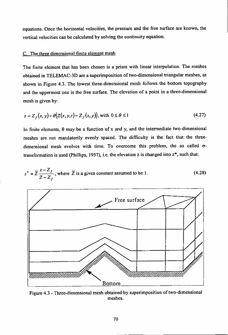
equations. Once the horizontal velocities, the pressure and the free surface are known, the
vertical velocities can be calculated by solving the continuity equation.
C. The three dimensional finite element mesh
The finite element that has been chosen is a prism with linear interpolation. The meshes
obtained in TELEMAC-3D are a superimposition o f two-dimensional triangular meshes, as
shown in Figure 4.3. The lowest three-dimensional mesh follows the bottom topography
and the uppermost one is the free surface. The elevation of a point in a three-dimensional
mesh is given by:
z = Z^{x,y)-^0[z{x,y,t)-Z^{x,y)), with 0 < ^ < 1 (4.27)
In finite elements, 0 may be a function of x and y, and the intermediate two-dimensional
meshes are not mandatorily evenly spaced. The difficulty is the fact that the three-
dimensional mesh evolves with time. To overcome this problem, the so called a-
transformation is used (Phillips, 1957), i.e. the elevafion z is changed into z*, such that:
z* = Z——-r-, where Z is a given constant assumed to be 1. Z - Z
(4.28)
Free surface
Bottom
Figure 4.3 - Three-dimensional mesh obtained by superimposition of two-dimensional meshes.
70
The c transformation method have also been used in other studies (Brenon & Le Hir,
1999) in order to avoid numerical artefacts due to large bathymetric gradients, especially
between the deep navigation channel and the shallow banks.
D. Definition of fiiction and turbulence
The law used to model bottom fiiction is a quadratic function of the flow, assuming a
turbulent boundary layer with a logarithmic profile. This law includes the representative
depth D o f bottom roughness (particle size), which can be related to the Chezy coefficient
by the equation:
C = 26.4 1/24
h''^ (4.29)
Modelling of turbulence was carried out by calculating the vertical viscosity and keeping
the horizontal one constant throughout the domain. The coefficient o f vertical viscosity or
diffusion of velocities and tracers is computed by TELEMAC-3D using the mixing length
theory, which takes into account density effects via a damping factor that depends on the
Richardson number {Ri), which is equivalent to taking vertical stratification due to salimty
or temperature into account.
Where:
/ and f r are the damping factors for velocity and tracer Im is the mixing length
]_dp
Ri^.g ^ (4.31)
TELEMAC-3D assumes the classical mixing length model, where Im is a function of the
water depth:
71
o I f z - Zy < 0.2h, then Im = K[Z - Zy ), where re = 0.41 is Karman's constant
o I f z - Zy > 0.2/1, then Im = O.ltdi
This method for modelling turbulence assumes that the horizontal gradients of w and v and
vertical gradients of w are neglected in favour of the vertical gradients of u and v in the
Reynolds equations. These fimctions are obtained on the assumption that there is local
equilibrium of turbulence, where local production and dissipation are in balance.
72
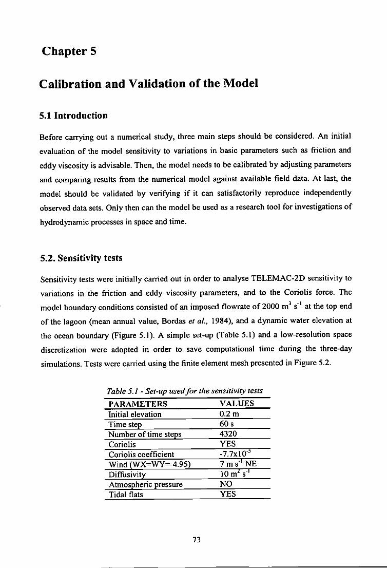
Chapter 5
Calibration and Validation of the Model
5.1 Introduction
Before carrying out a numerical study, three main steps should be considered. An initial
evaluation of the model sensitivity to variations in basic parameters such as friction and
eddy viscosity is advisable. Then, the model needs to be calibrated by adjusting parameters
and comparing results from the numerical model against available field data. At last, the
model should be validated by verifying i f it can satisfactorily reproduce independently
observed data sets. Only then can the model be used as a research tool for investigations of
hydrodynamic processes in space and time.
5.2. Sensitivity tests
Sensitivity tests were initially carried out in order to analyse TELEMAC-2D sensitivity to
variations in the friction and eddy viscosity parameters, and to the Coriolis force. The
model boundary conditions consisted of an imposed flowrate of 2000 m^ s * at the top end
of the lagoon (mean annual value, Bordas et aL, 1984), and a dynamic water elevation at
the ocean boundary (Figure 5,1). A simple set-up (Table 5.1) and a low-resolution space
discretization were adopted in order to save computational time during the three-day
simulations. Tests were carried using the finite element mesh presented in Figure 5.2.
Table 5.1 - Set-up used for the sensitivity tests
PARAMETERS VALUES Initial elevation 0.2 m Time step 60 s Number of time steps 4320 Coriolis YES Coriolis coefficient -7.7x10'"* Wind (WX=WY=-4.95) 7 m s"* NE Difflisivity 10 m^ s ' Atmospheric pressure NO Tidal flats YES
73
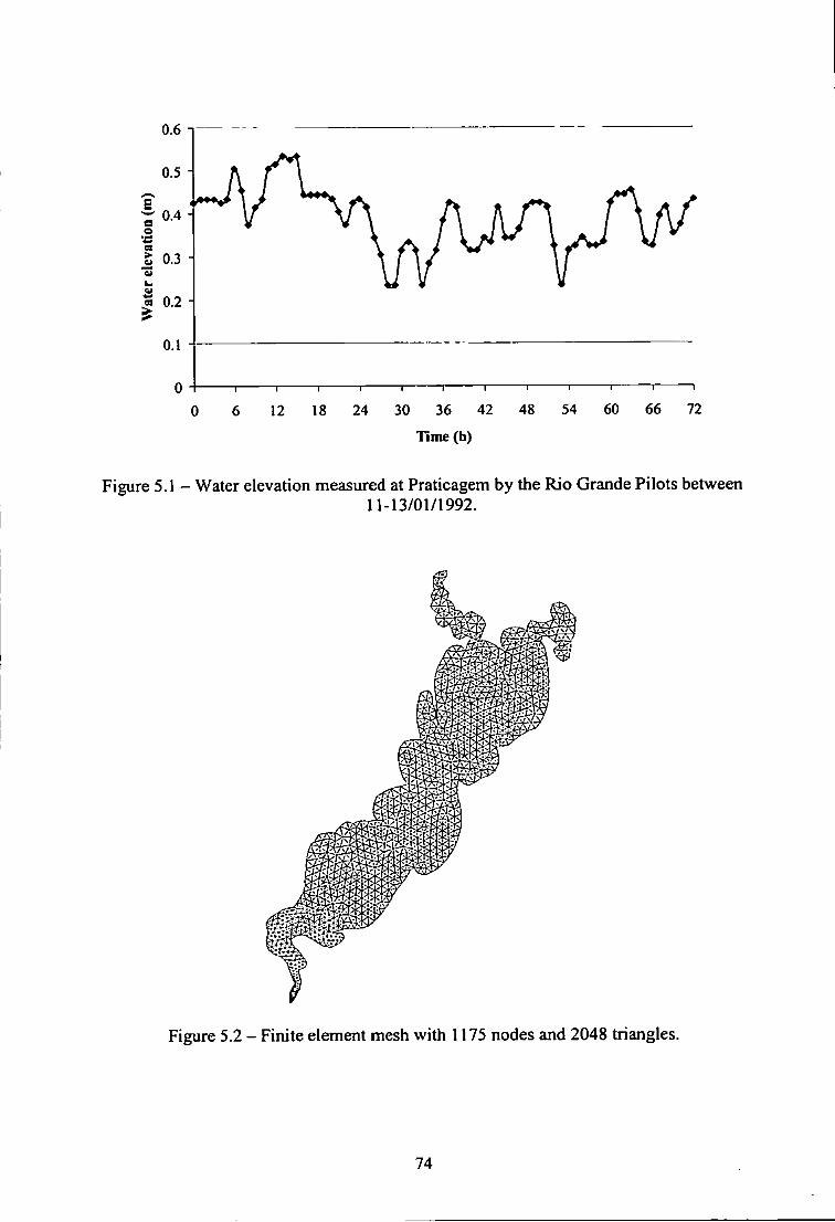
« 0.2
60 66 30 36 42 48
Time (h)
Figure 5.1 - Water elevation measured at Praticagem by the Rio Grande Pilots between 11-13/01/1992.
Figure 5.2 - Finite element mesh with 1175 nodes and 2048 triangles.
74
In order to investigate the model sensitivity to different laws of bottom fiiction and to a
range of values for the fiiction coefficient found in the literature, fiiction sensitivity tests
were carried out by applying the Manning, Chezy and Nikuradse laws. Table 5.2 shows a
summary of the fiiction sensitivity tests.
Table 5.2 - Friction sensitivity tests
Name of the test Friction coefficient Maiming 1 m=0.040 Manning2 m=0.025 Manning3 m=0.015 Chezyl C=37 Chezy2 C=65 Chezy3 C=100 Nikuradse 1 Ks=0.001 (smooth mud) Nikuradse2 Ks=0.01 Nikuradse3 Ks=0.1 (sand)
Figure 5.3 illustrates the effect of varying the law of bottom fiiction and the value of the
fiiction coefficient on the longitudinal velocity at Praticagem, It is clear that the overall
variation of the longitudinal velocity is independent of which definition of bottom fiiction
is assumed, although its magnitude is controlled by the magnitude of the fiiction
coefficient. Figure 5.4 shows the fiiction effect on the circulation pattern of the Patos
Lagoon when applying different values of the Chezy fiiction coefficient. Results indicate
that the general patterns of water movement are comparable and the velocity magnitude
increases accordingly to the fiiction coefficient variation.
Sensitivity tests on eddy viscosity were carried out based on the same initial and boundary
conditions, and applying the Maiming law of bottom fiiction (m=0.025). Very little
difference was observed in the predicted circulation pattern for eddy viscosity coefficients
varying from ^^=0.01 to We=100 m^ s"' (Figure 5.5). Attenuation of the flow pattern was
observed only when applying Ve=1000 m^ s"'. These results indicate that eddy viscosity has
little effect on the lagoon circulation, which seems to be mainly controlled by topography
and advective processes.
Although the Patos Lagoon is a huge water body, it is much longer than it is wide, and the
Coriolis force is not expected to be significant. In order to analyse the Coriolis effect on
the lagoon circulation, the Manning2 test (Table 5.2 - ;n=0.025) was repeated without
taking into account the Coriolis force. No difference was observed when comparing
75
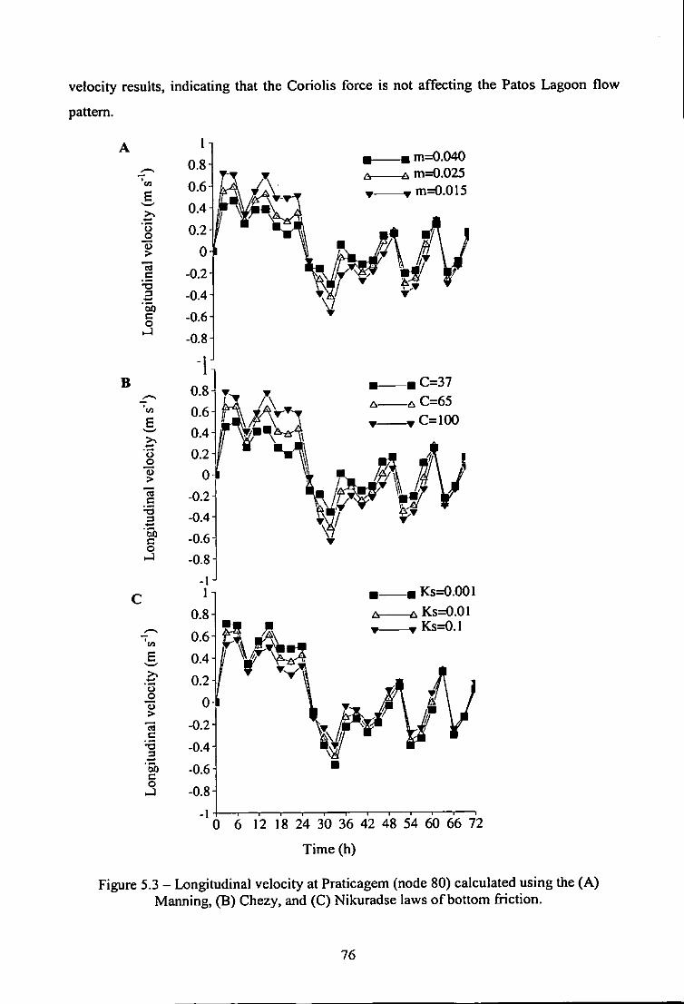
velocity results, indicating that the Coriolis force is not affecting the Patos Lagoon flow
pattern.
o
> c
"•5 3 '5b c o
B
(A
"u
00 c o
H4
8 >
c '•a 3
'5b c o
_ m=0.040 ^ A m=0.025 ^ y m=0.015
C=37
C=100
Ks=0.001 ^ Ks=0.01
- vKs=0.1
0 6 12 18 24 30 36 42 48 54 60 66 72
Time (h)
Figure 5.3 - Longitudinal velocity at Praticagem (node 80) calculated using the (A) Manning, (B) Chezy, and (C) Nikuradse laws of bottom friction.
76
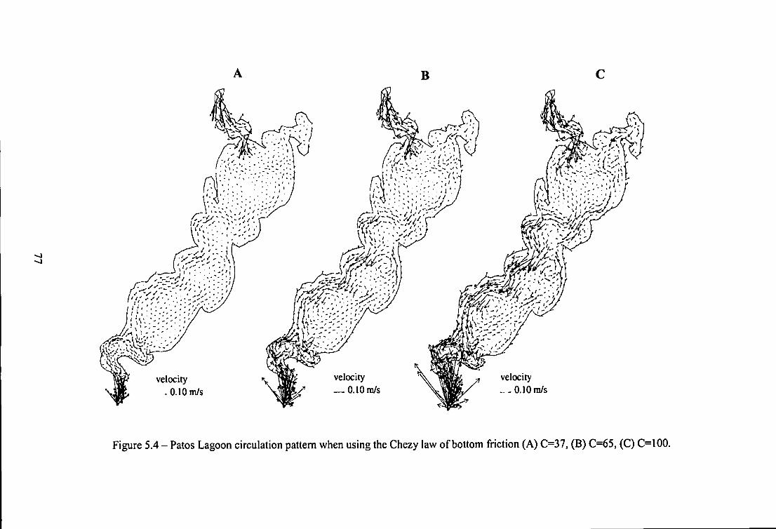
B
Pi
velocity O.lOra/s
velocity .O.lOm/s
velocity -^O.lOm/s
Figure 5.4 - Patos Lagoon circulation pattern when using the Chezy law of bottom friction (A) C=37, (B) C=65, (C) C=100.
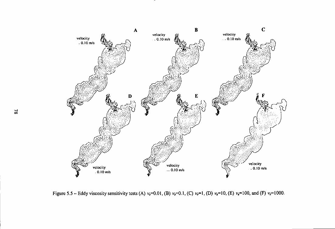
00
velocity . 0.10 m/s
velocity 0.10 ra/s
velocity 0.10 m/s
velocity velocity 0.10 m/s 0.10 m/s
-i - velocity .0.10 m/s
Figure 5.5-Eddy viscosity sensitivity tests (A) ^,=0.01,(8) v,=0.1,(C) v,=l , (D) K.=10,(E) V,=100, and (F) v^=100a
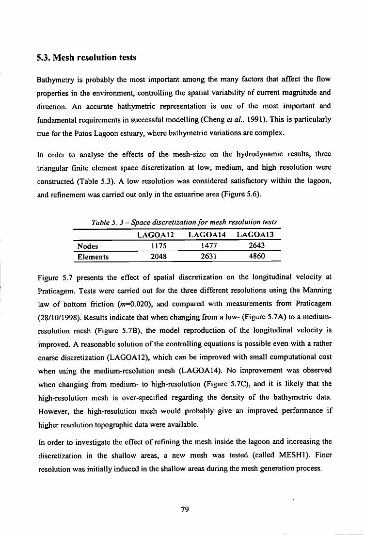
5.3. Mesh resolution tests
Bathymetry is probably the most important among the many factors that affect the flow
properties in the environment, controlling the spatial variability of current magnitude and
direction. An accurate bathymetric representation is one of the most important and
fundamental requirements in successful modelling (Cheng et al., 1991). This is particularly
true for the Palos Lagoon estuary, where bathymetric variations are complex.
In order to analyse the effects of the mesh-size on the hydrodynamic results, three
triangular finite element space discretization at low, medium, and high resolution were
constructed (Table 5.3). A low resolution was considered satisfactory within the lagoon,
and refinement was carried out only in the estuarine area (Figure 5.6).
Table 5. 3- Space discretization for mesh resolution tests
LAGOA12 LAGOA14 LAGOA13
Nodes 1175 1477 2643 Elements 2048 2631 4860
Figure 5.7 presents the effect of spatial discretization on the longitudinal velocity at
Praticagem. Tests were carried out for the three different resolutions using the Manning
law of bottom friction (w2=0.020), and compared with measurements from Praticagem
(28/10/1998). Results indicate that when changing from a low- (Figure 5.7A) to a medium-
resolution mesh (Figure 5,7B), the model reproduction of the longitudinal velocity is
improved. A reasonable solution of the controlling equations is possible even with a rather
coarse discretization (LAG0A12), which can be improved with small computational cost
when using the medium-resolution mesh (LAGOA14). No improvement was observed
when changing from medium- to high-resolution (Figure 5.7C), and it is likely that the
high-resolution mesh is over-specified regarding the density of the bathymetric data.
However, the high-resolution mesh would probably give an improved performance i f
higher resolution topographic data were available.
In order to investigate the effect of refining the mesh inside the lagoon and increasing the
discretization in the shallow areas, a new mesh was tested (called MESHl) . Finer
resolution was initially induced in the shallow areas during the mesh generation process.
79
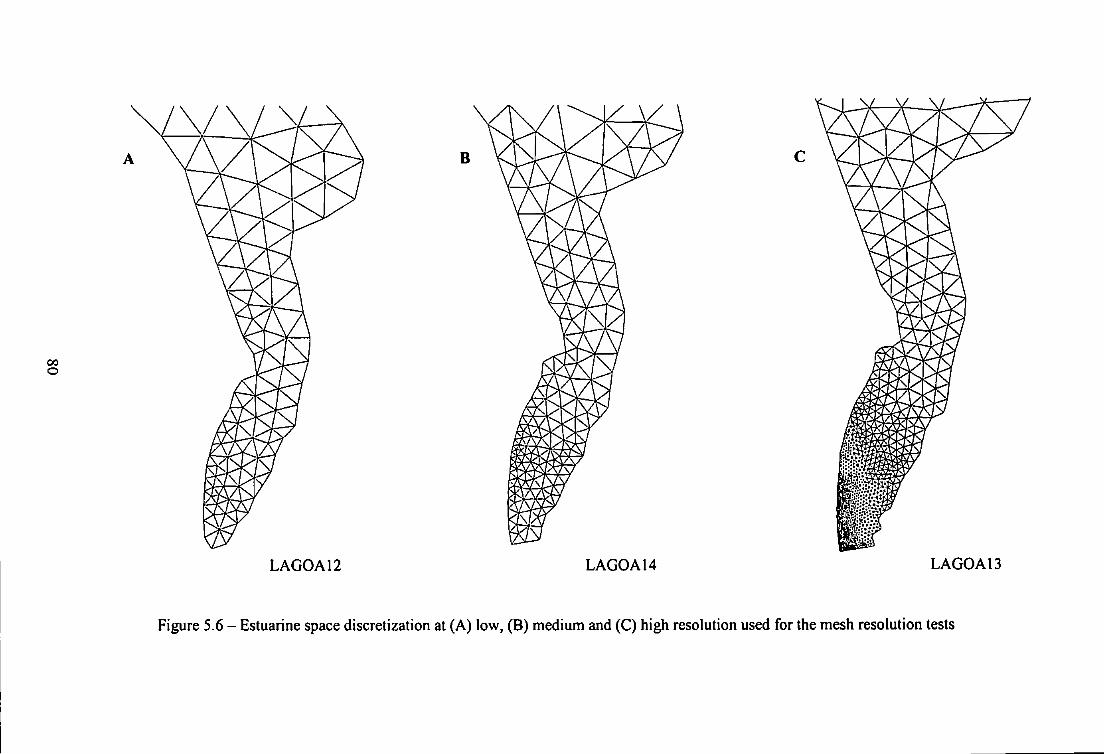
00 o
LAG0A12 LAG0A14 LAG0A13
Figure 5.6 - Estuarine space discretization at (A) low, (B) medium and (C) high resolution used for the mesh resolution tests
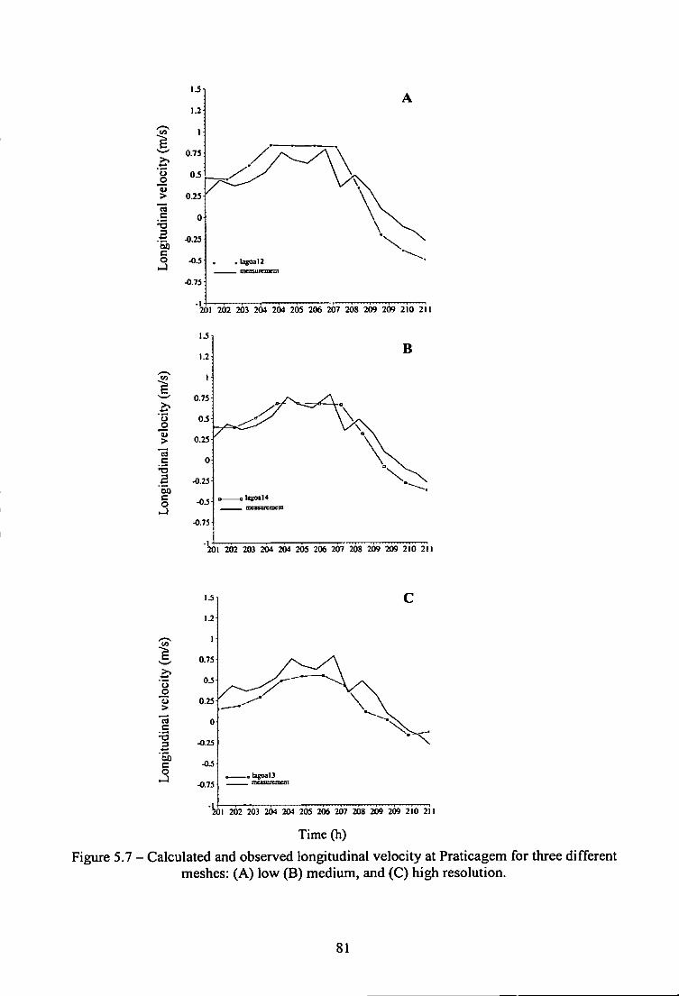
I
1 a c 1 5b § lagoal2
201 202 203 20* 204 205 206 207 208 209 209 210 211
1 o O 1 .c -5 B
2
1.2
1
0.75
OJ
0.25
0
^.25
-OJ
-0.75
B
^ —
o 0 lagoaM mciniftnictii
201 202 203 204 204 205 206 207 208 209 209 210 211
I > .c •5 3 DO C P
I J
1.2
1
0.75
OJ
0.25
0
-025
-OJ
-0.75
<1
la£(nl3
201 202 203 204 204 205 206 207 208 209 209 210 211
Time (h)
Figure 5.7 - Calculated and observed longitudinal velocity at Praticagem for three different meshes: (A) low (B) medium, and (C) high resolution.
81
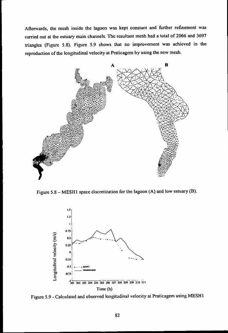
Afterwards, the mesh inside the lagoon was kept constant and further refinement was
carried out at the estuary main channels. The resultant mesh had a total of 2066 and 3697
triangles (Figure 5.8). Figure 5.9 shows that no improvement was achieved in the
reproduction of the longitudinal velocity at Praticagem by using the new mesh.
Figure 5.8 - MESHl space discretization for the lagoon (A) and low estuary (B).
o o
1 'a c 1 E3) c o
201 202 203 204 2CM 205 206 207 208 209 209 210 211
Time (h)
Figure 5.9 - Calculated and observed longitudinal velocity at Praticagem using MESHl
82
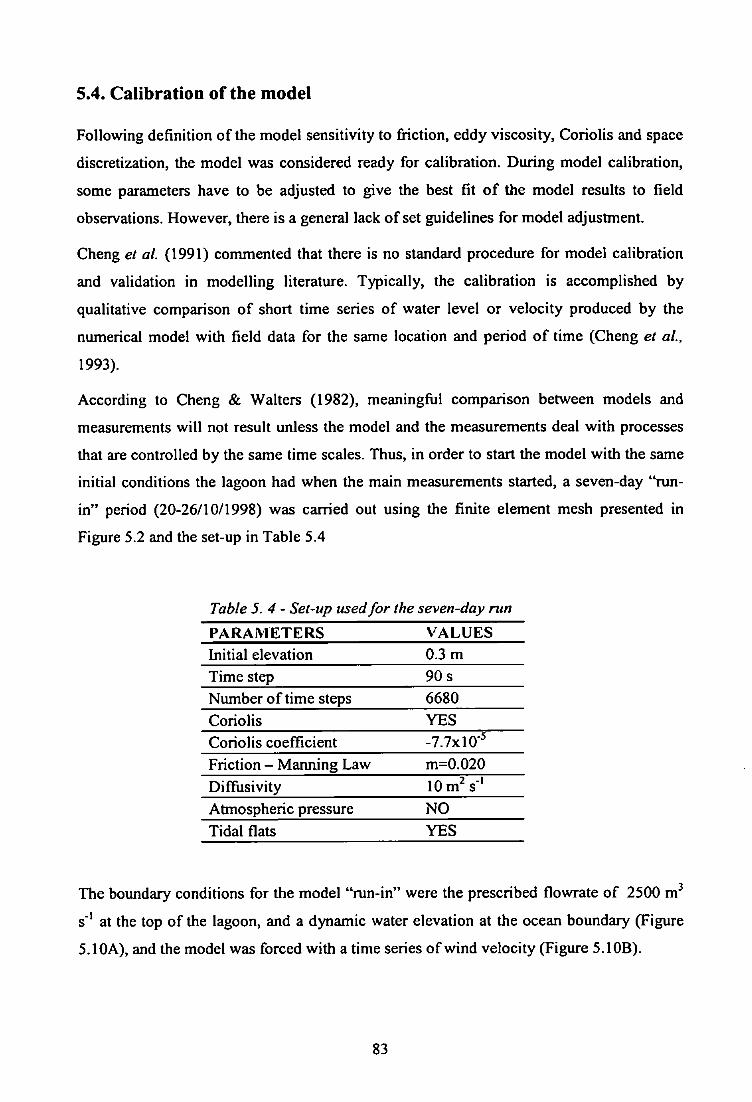
5.4. Calibration of the model
Following definition of the model sensitivity to friction, eddy viscosity, Coriolis and space
discretization, the model was considered ready for calibration. During model calibration,
some parameters have to be adjusted to give the best fit o f the model results to field
observations. However, there is a general lack of set guidelines for model adjustment.
Cheng et al. (1991) commented that there is no standard procedure for model calibration
and validation in modelling literature. Typically, the calibration is accomplished by
qualitative comparison of short time series of water level or velocity produced by the
numerical model with field data for the same location and period o f time (Cheng et ai,
1993).
According to Cheng & Walters (1982), meaningful comparison between models and
measurements wi l l not result unless the model and the measurements deal with processes
that are controlled by the same time scales. Thus, in order to start the model with the same
initial conditions the lagoon had when the main measurements started, a seven-day "run-
in" period (20-26/10/1998) was carried out using the finite element mesh presented in
Figure 5.2 and the set-up in Table 5.4
Table 5. 4 - Set-up used for the seven-day run
PARAMETERS VALUES Initial elevation 0.3 m Time step 90 s Number of time steps 6680 Coriolis YES Coriolis coefficient -7.7x10'^ Friction - Manning Law m=0.020 Diffiisivity lOm^ s ' Atmospheric pressure NO Tidal flats YES
The boundary conditions for the model "nin-in" were the prescribed flowrate of 2500 m"*
s" at the top of the lagoon, and a dynamic water elevation at the ocean boundary (Figure
5.10A), and the model was forced with a time series of wind velocity (Figure 5.10B).
83
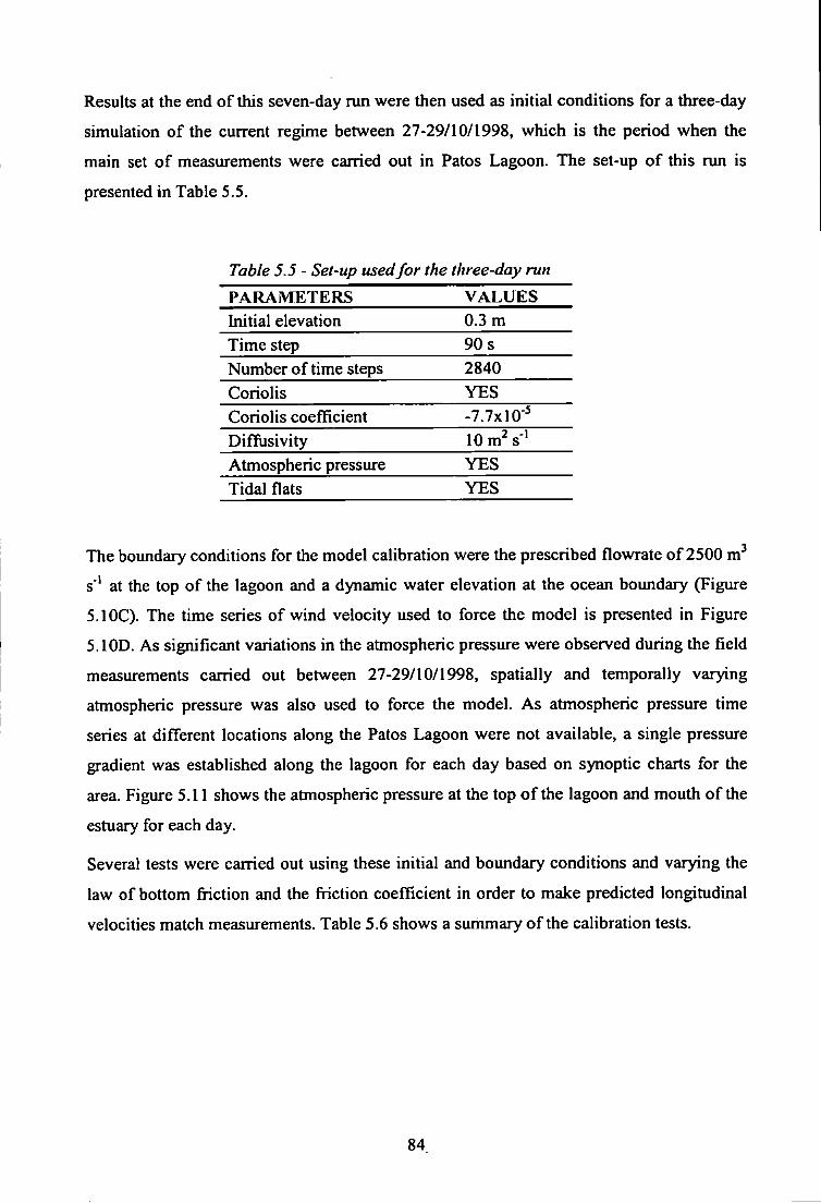
Results at the end of this seven-day run were then used as initial conditions for a three-day
simulation of the current regime between 27-29/10/1998, which is the period when the
main set of measurements were carried out in Patos Lagoon. The set-up of this run is
presented in Table 5.5.
Table 5.5 - Set-up used for the three-day run
PARAMETERS VALUES Initial elevation 0.3 m Time step 90 s Number of time steps 2840 Coriolis YES Coriolis coefficient -7.7x10"^ Difflisivity 10 m^ s * Atmospheric pressure YES Tidal flats YES
The boundary conditions for the model calibration were the prescribed flowrate of 2500 m^
s" at the top of the lagoon and a dynamic water elevation at the ocean boundary (Figure
5.IOC). The time series of wind velocity used to force the model is presented in Figure
5.10D, As significant variations in the atmospheric pressure were observed during the field
measurements carried out between 27-29/10/1998, spatially and temporally varying
atmospheric pressure was also used to force the model. As atmospheric pressure time
series at different locations along the Patos Lagoon were not available, a single pressure
gradient was established along the lagoon for each day based on synoptic charts for the
area. Figure 5.11 shows the atmospheric pressure at the top o f the lagoon and mouth of the
estuary for each day.
Several tests were carried out using these initial and boundary conditions and varying the
law of bottom friction and the fiiction coefficient in order to make predicted longitudinal
velocities match measurements. Table 5.6 shows a summary of the calibration tests.
84
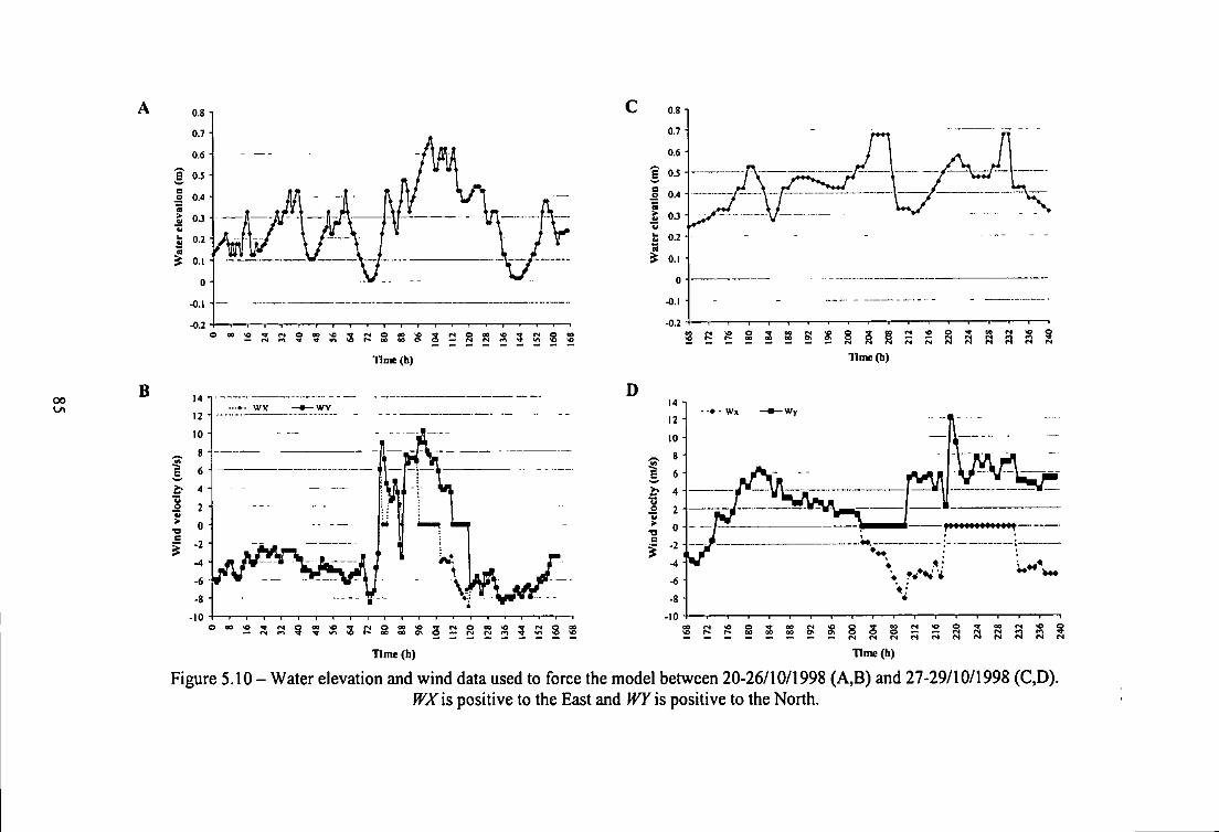
00 B
E 0.5
Tlnie(h)
^ V *n
Time (h)
0.7
0.6
I 0.5
J 0.4
t 03 t 0.2
I 0.,
0
-0.1
-0.2
S « I 3 S § a Tlme(h)
D
r ) M (N r j M a a a a a s Tlmcih)
Figure 5.10 - Water elevation and wind data used to force the model between 20-26/10/1998 (A,B) and 27-29/10/1998 (C,D). WXis positive to the East and WY is positive to the North.
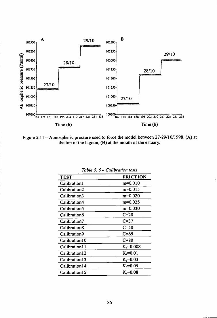
u
I i CO C/5
i O E
102500
102250
102000
101750
101500
IOI250
101000
100750
100500
29/10
28/10
27/10
167 174 181 188 195 203 210 217 224 231 238
Time (h)
102500
102250
102000
101750
101500
101250
101000
100750
B
100500
28/10
27/10
29/10
167 174 181 188 195 203 210 217 224 231 238
Time (h)
Figure 5.11 - Atmospheric pressure used to force the model between 27-29/10/1998. (A) at the top of the lagoon, (B) at the mouth o f the estuary.
Table 5.6- Calibration tests
TEST FRICTION Calibration! m=0.010 Calibration2 m=0.015 Calibrations m=0.020 Calibration4 m=0.025 Calibrations m=0.030 Calibration6 C=20 Calibration7 C=37 Calibrations C=50 Calibration9 C=65 Calibration! 0 C=80 Calibration! 1 Ks=0.008 Calibration 12 K5=0.01 Calibration 13 Ks=0.03 Calibration! 4 Ks=0.05 Calibration! 5 Ks=0.08
86
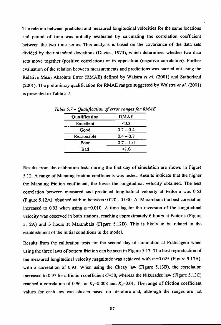
The relation between predicted and measured longitudinal velocities for the same locations
and period of time was initially evaluated by calculating the correlation coefficient
between the two time series. This analysis is based on the covariance o f the data sets
divided by their standard deviations (Davies, 1973), which determines whether two data
sets move together (positive correlation) or in opposition (negative correlation). Further
evaluation of the relation between measurements and predictions was carried out using the
Relative Mean Absolute Error (RMAE) defined by Walstra et ai (2001) and Sutheriand
(2001). The preliminary quaUfication for RMAE ranges suggested by Walstra et al. (2001)
is presented in Table 5.7.
Table 5.7 - Qualification of error ranges for RMAE
Qualification RMAE Excellent <0.2
Good 0.2-0.4 Reasonable 0.4-0.7
Poor 0.7-1.0 Bad >l.O
Results fi-om the calibration tests during the first day of simulation are shown in Figure
5.12. A range o f Manning friction coefficients was tested. Results indicate that the higher
the Manning finction coefficient, the lower the longitudinal velocity obtained. The best
correlation between measured and predicted longitudinal velocity at Feitoria was 0,53
(Figure 5.12A), obtained with m between 0.020 - 0.030. At Marambaia the best correlation
increased to 0.93 when using /7/=0.010. A time lag for the reversion of the longitudinal
velocity was observed in both stations, reaching approximately 6 hours at Feitoria (Figure
5.12A) and 3 hours at Marambaia (Figure 5.12B). This is likely to be related to the
establishment of the initial conditions in the model.
Results fi-om the calibration tests for the second day of simulation at Praticagem when
using the three laws of bottom fiiction can be seen in Figure 5.13. The best reproduction of
the measured longitudinal velocity magnitude was achieved with /n=0.025 (Figure 5.13A),
with a correlation of 0.93. When using the Chezy law (Figure 5.13B), the correlation
increased to 0.97 for a fiiction coefficient C=50, whereas the Nikuradse law (Figure 5.13C)
reached a correlation of 0.96 for Ks=O.OQ% and / l j=0 .01 . The range o f fiiction coefficient
values for each law was chosen based on literature and, although the ranges are not
87
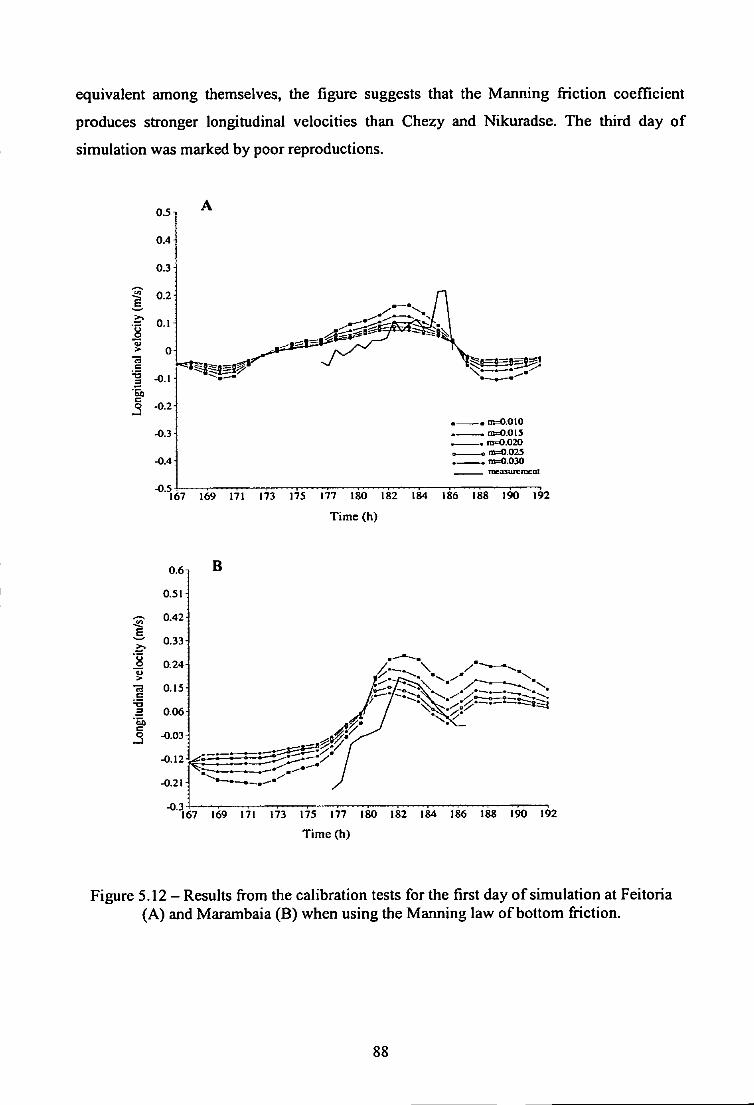
equivalent among themselves, the figure suggests that the Manning friction coefficient
produces stronger longitudinal velocities than Chezy and Nikuradse. The third day of
simulation was marked by poor reproductions.
0.5
0.4-1
0.3
0.2
O.I
0
-0.1
-0.2
^.3
-0.4 H
-0.5
.« [n=0.010 ^ ro=0.015
m=0.020 ^m=0.025 ^ m=0.030 _ mcasurcmcnl
167 169 171 173 175 177 180 182 184 186 188 190 192
Time (h)
0.42^
0. 5H
0.06 H
-0.03 d
-0. 2
-0.3 167 169 171 173 175 177 180 182 184 186 188 190 192
Time (h)
Figure 5.12 - Results from the calibration tests for the first day of simulation at Feitoria (A) and Marambaia (B) when using the Manning law of bottom friction.
88
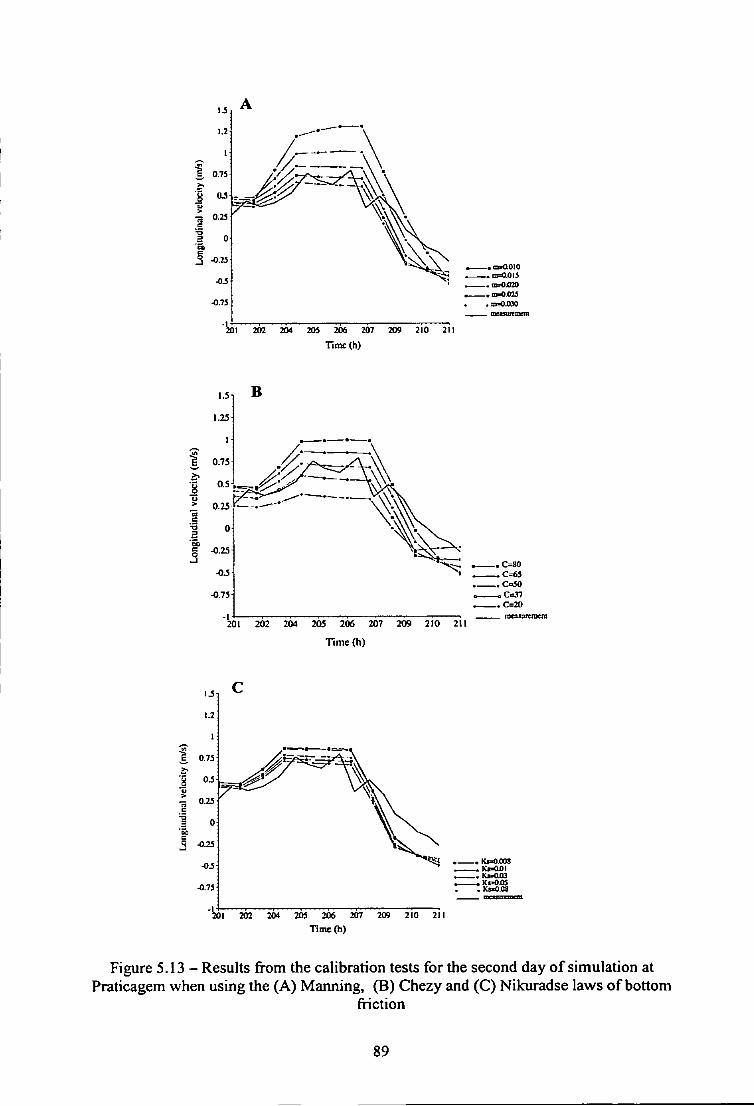
.n>-0i l30
202 204 205 206 207 209 210 211 riin£(h)
,C=80 ,C=65 ,C=30 .C=37 .C=20
201 202 2W 205 206 207 209 210 211
Time (h)
B 0.75
Kt=0XJ03
-K*=aoi K«=0 05
202 204 20S 206 207 209 210 211 TimeOi)
Figure 5.13 - Results fi*om the calibration tests for the second day of simulation at Praticagem when using the (A) Manning, (B) Chezy and (C) Nikuradse laws of bottom
friction
89
Although the model reproduces reasonably well the longitudinal velocity measured at the
three stations during the first two days, it was not able to reproduce the observed lateral
velocities (not shown). Several limitations in the model and data set can explain why a
better reproduction was not achieved overall: 1) wind data was prescribed at Praticagem
and considered constant throughout the lagoon; 2) water elevation data was measured only
during the day-time and interpolated for the night period; 3) the resolution of the
bathymetric data and the distortion produced by the grid size; 4) salinity stratification was
observed in the lower estuary during the measurements, but was not talcen into account in
the model; and 5) the model predicts depth-averaged velocities, whereas measurements are
for a particular depth.
However, a comparison between measurements carried out at a shallow area around
Feitoria between 26-28/10/1998 using a self-recording current meter moored overnight
with calculated results for the same location and period of time when using the Maruiing
law of bottom friction (m=0.020) shows a different result. A better reproduction of the
lateral velocities for the three overnight periods was achieved (Figure 5.14).
Although it is known that, in principle, the friction coefficient should change according to
the nature of the bed (Aldridge & Davies, 1993), numerical models are generally run with
uniform values of bed friction. Smith & Cheng (1987) and Cheng et al. (1993) tested
spatially varying friction by applying the Chezy and Manning laws of bottom friction,
respectively. They both found that the introduction of depth dependent friction was
necessary to achieve a best fit to the available field data.
The effect of varying bed friction in space as a function of bed composition is investigated
here. The Nikiu-adse law of bottom friction was chosen because it prescribes the grain size
at the bottom in the friction coefficient. The lagoon shallow areas have a sandy bed, the
main lagoon has silt bed, and the deeper channels vary from fine silt to mud. Thus different
friction coefficients were specified for specific depth ranges (Table 5.8). The distribution
of the friction coefficient throughout the lagoon is presented in Figure 5.15.
90
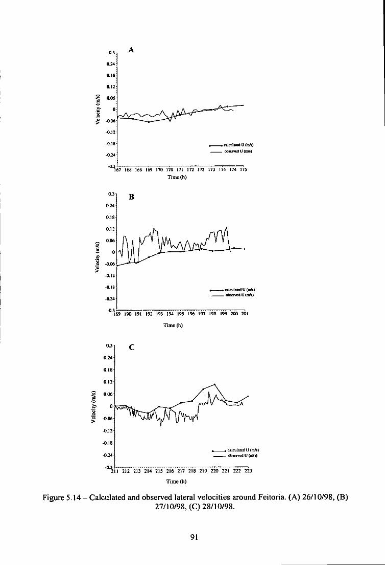
0.3
0.24
a i8
a i2
1 0.06
0
1 > -0.06
-0.12
-0.18
-0.24
•03
. calcuUued U (m/it
167 168 168 169 170 170 171 172 172 173 174 174 175
Time(h)
ctlculucd U (m/i) obsavta U imli)
-0.3 189 190 191 192 193 194 195 196 197 198 199 200 20)
Time (h)
0.3
0.24
0.18
0.12
0.06
0
« -0.06
-0.12
-0.18
-0.24
-0.3
. calnilalcd U (m/i) Observed U (m/i)
211 212 213 214 215 216 217 218 219 220 221 222 223
Time (h)
Figure 5.14 - Calculated and observed lateral velocities around Feitoria. (A) 26/10/98, (B) 27/10/98, (C) 28/10/98.
91
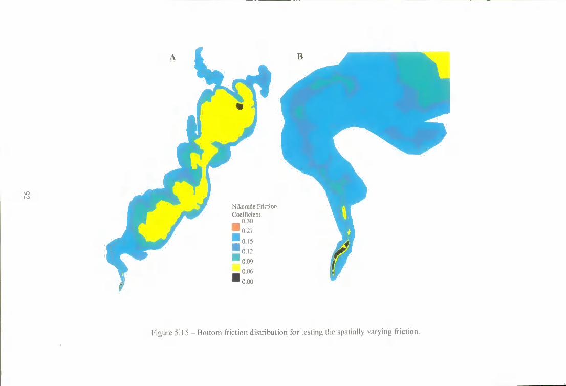
t J Nikurade Fnctu Coefficient
0.30 0.27
0.15
0.12 0.09 0.06 0.00
Mgure 5.15 - Bottom friction distribution for testing the spatially varying friction.
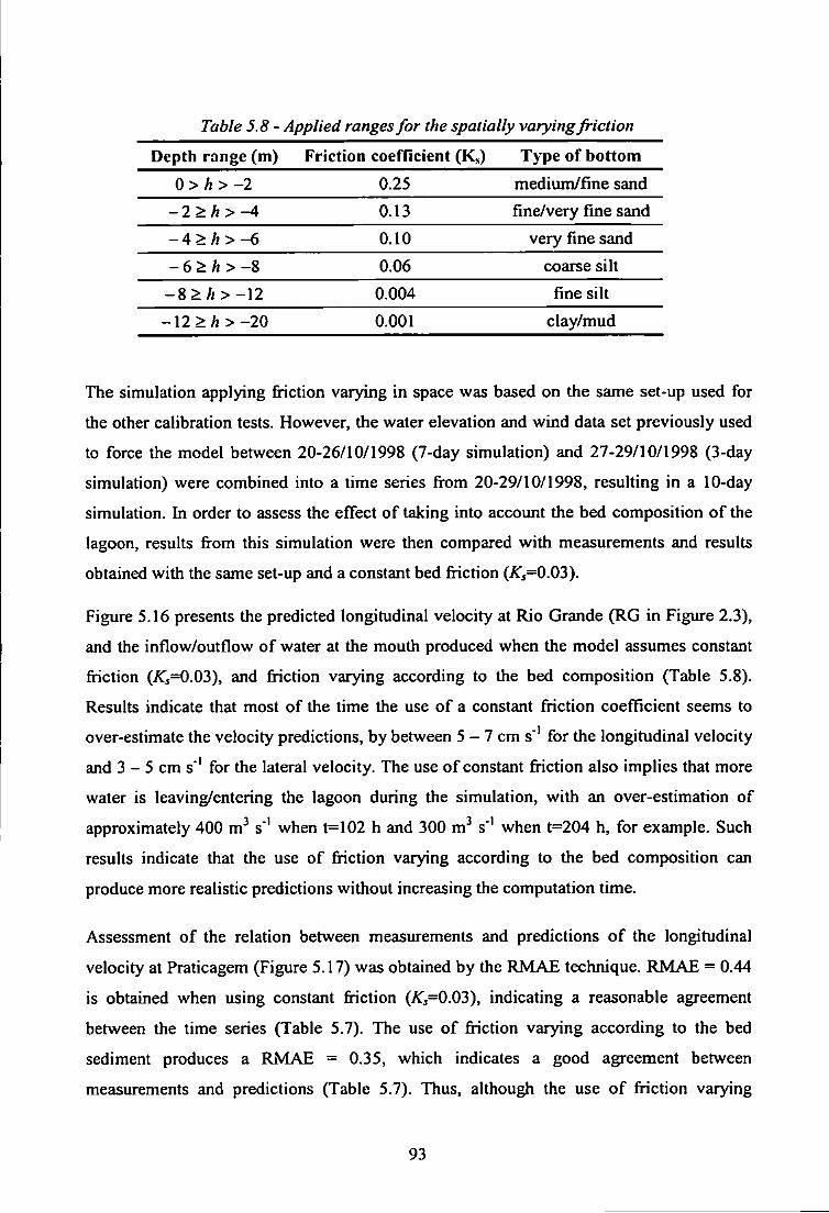
Table 5.8- Applied ranges for the spatially varying friction
Depth range (m) Friction coefficient (Ks) Type of bottom
0 > / i > -2 0.25 medium/fine sand
-2>h>-A 0.13 fine/very fine sand
-A>h>-6 0.10 very fine sand
-6>h>-S 0.06 coarse silt
- 8 > / i > - 1 2 0.004 fine silt
- 1 2 > A > - 2 0 0.001 clay/mud
The simulation applying finction varying in space was based on the same set-up used for
the other calibration tests. However, the water elevation and wind data set previously used
to force the model between 20-26/10/1998 (7-day simulation) and 27-29/10/1998 (3-day
simulation) were combined into a time series fi*om 20-29/10/1998, resulting in a 10-day
simulation. In order to assess the effect of taking into account the bed composition of the
lagoon, results fi-om this simulation were then compared with measurements and results
obtained with the same set-up and a constant bed finction (^5=0.03).
Figure 5.16 presents the predicted longitudinal velocity at Rio Grande (RG in Figure 2.3),
and the inflow/outflow of water at the mouth produced when the model assumes constant
fiiction {Ks=0.03), and fiiction varying according to the bed composition (Table 5.8).
Results indicate that most of the time the use of a constant fiiction coefficient seems to
over-estimate the velocity predictions, by between 5 - 7 cm s " for the longitudinal velocity
and 3 - 5 cm s * for the lateral velocity. The use of constant fiiction also implies that more
water is leaving/entering the lagoon during the simulation, with an over-estimation of
approximately 400 m"* s'' when t=102 h and 300 m^ s"' when t=204 h, for example. Such
results indicate that the use of fiiction varying according to the bed composition can
produce more realistic predictions without increasing the computation time.
Assessment of the relation between measurements and predictions of the longitudinal
velocity at Praticagem (Figure 5.17) was obtained by the RMAE technique. RMAE = 0.44
is obtained when using constant fiiction (/G=0.03), indicating a reasonable agreement
between the time series (Table 5.7). The use of fiiction varying according to the bed
sediment produces a RMAE = 0.35, which indicates a good agreement between
measurements and predictions (Table 5.7). Thus, although the use of fiiction varying
93
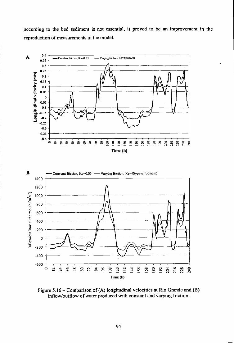
according to the bed sediment is not essential, it proved to be an improvement in the
reproduction of measurements in the model.
— Varying reton, Ks=fbotiDnv Constaa fiKOon, Ks=0.03
Time (h)
B Constant friction, Ks=0.03 Vaiying friction, Ks=fl;type of bottom) 1400
t3 400
200 i
VO OO O ( N */-! VO OO S 2 S ?
O J ( N ( N
Time (h)
Figure 5.16 - Comparison of (A) longitudinal velocities at Rio Grande and (B) inflow/outflow of water produced with constant and varying fiiction.
94
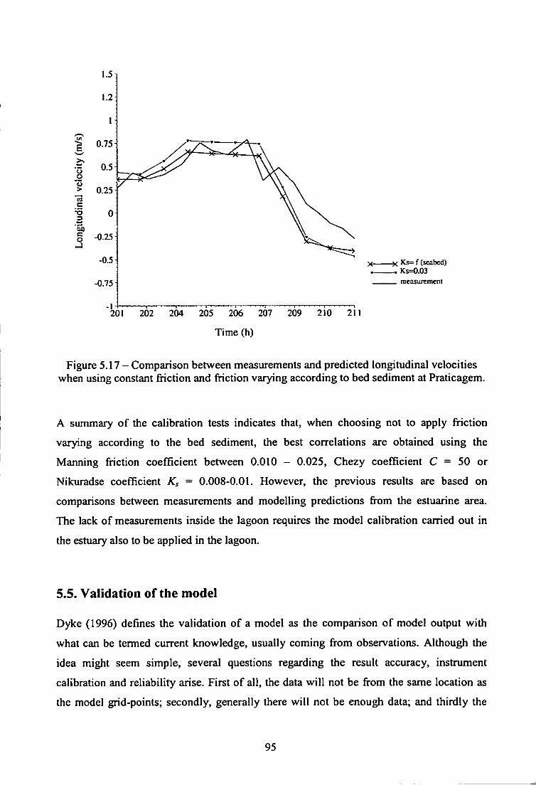
•a 3 to c
0.25 ^
-0.25 H
-X Ks=f (seabed) Ks=0.03 measurement
201 202 204 205 206 207 209 210 211
Time (h)
Figure 5.17 - Comparison between measurements and predicted longitudinal velocities when using constant friction and friction varying according to bed sediment at Praticagem.
A summary of the calibration tests indicates that, when choosing not to apply friction
varying according to the bed sediment, the best correlations are obtained using the
Manning friction coefficient between 0.010 - 0.025, Chezy coefficient C = 50 or
Nikuradse coefficient Ks = 0.008-0.01. However, the previous results are based on
comparisons between measurements and modelling predictions from the estuarine area.
The lack of measurements inside the lagoon requires the model calibration carried out in
the estuary also to be applied in the lagoon.
5.5. Validation of the model
Dylce (1996) defines the validation of a model as the comparison of model output with
what can be termed current knowledge, usually coming from observations. Although the
idea might seem simple, several questions regarding the result accuracy, instrument
calibration and reliability arise. First of all, the data wi l l not be from the same location as
the model grid-points; secondly, generally there wi l l not be enough data; and thirdly the
95
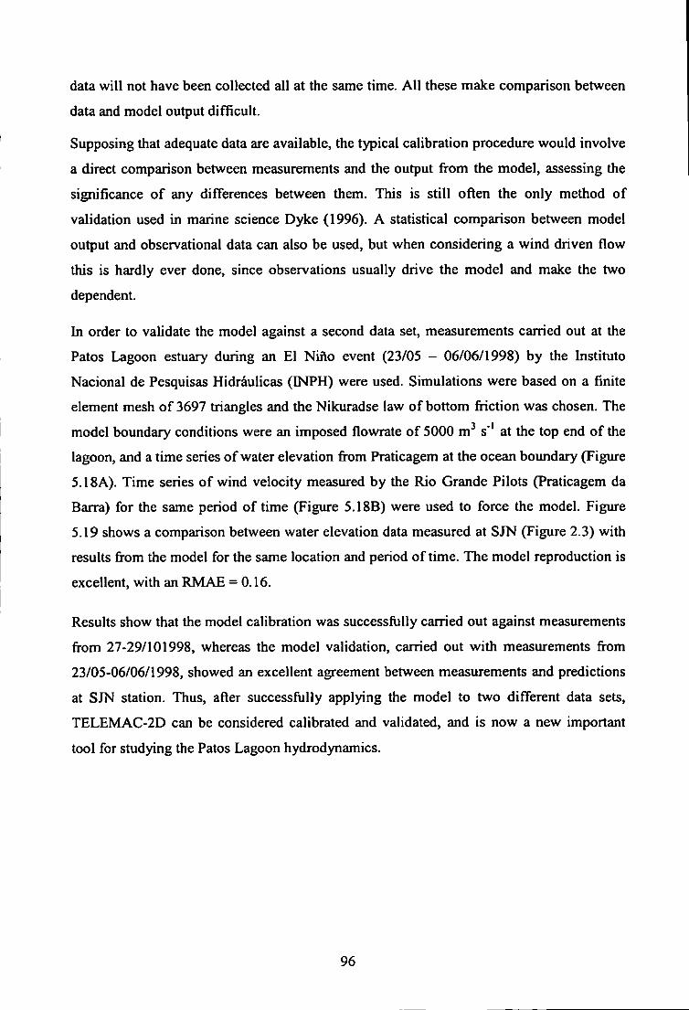
data will not have been collected all at the same time. All these make comparison between
data and model output difficult.
Supposing that adequate data are available, the typical calibration procedure would involve
a direct comparison between measurements and the output from the model, assessing the
significance of any differences between them. This is still often the only method of
validation used in marine science Dyke (1996). A statistical comparison between model
output and observational data can also be used, but when considering a wind driven flow
this is hardly ever done, since observations usually drive the model and make the two
dependent.
hi order to validate the model against a second data set, measurements carried out at the
Patos Lagoon estuary during an El Nino event (23/05 - 06/06/1998) by the Instituto
Nacional de Pesquisas Hidrdulicas (INPH) were used. Simulations were based on a finite
element mesh of 3697 triangles and the Nikuradse law of bottom friction was chosen. The
model boundary conditions were an imposed flowrate of 5000 m"* s * at the top end of the
lagoon, and a time series of water elevation from Praticagem at the ocean boundary (Figure
5.18A). Time series of wind velocity measured by the Rio Grande Pilots (Praticagem da
Barra) for the same period of time (Figure 5.18B) were used to force the model. Figure
5.19 shows a comparison between water elevation data measured at SJN (Figure 2.3) with
results from the model for the same location and period of time. The model reproduction is
excellent, with an RMAE = 0.16.
Results show that the model calibration was successfully carried out against measurements
from 27-29/101998, whereas the model validation, carried out with measurements from
23/05-06/06/1998, showed an excellent agreement between measurements and predictions
at SJN station. Thus, after successfully applying the model to two different data sets,
TELEMAC-2D can be considered calibrated and validated, and is now a new important
tool for studying the Patos Lagoon hydrodynamics.
96
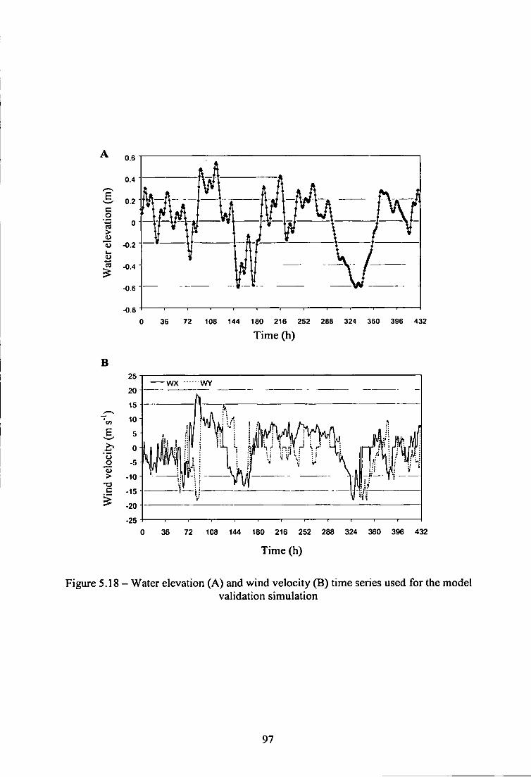
B
U O f c
-0.8 36 72 108 144 180 216 252 2B8 324 360 396 432
Time (h)
J
36 72 IDS 144 180 216 252 288 324 360 396 432
Time (h)
Figure 5.18 - Water elevation (A) and wind velocity (B) time series used for the model validation simulation
97
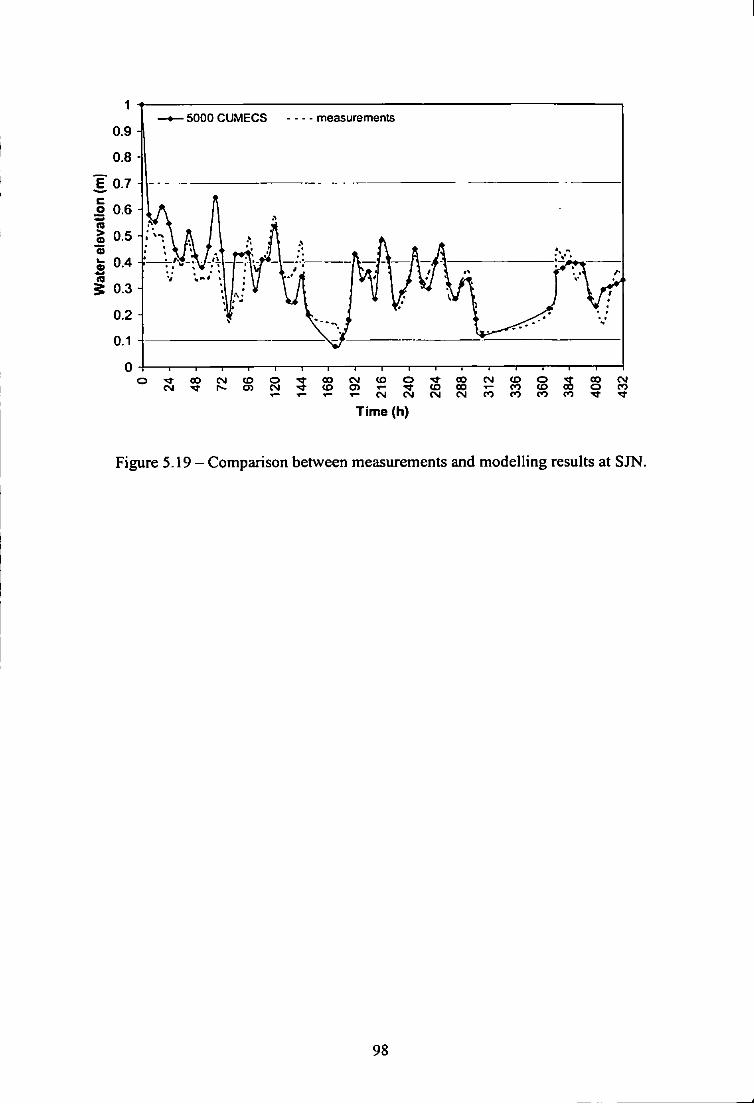
5000 CUMECS measurements
00 CM T j -
CNJ CD CM CD CM CD r - O ^ C M - ^ C D O ^ T - T j - C D O O - ^ f O C D C O O r O T - ^ - < - ^ C M C M C M C M C 0 C 0 C O n T r T t
Time (h)
Figure 5.19 - Comparison between measurements and modelling results at SJN.
98
Chapter 6
The Patos Lagoon Two-dimensional Circulation
6.1. Introduction
This chapter presents several numerical experiments carried out using the TELEMAC-2D
model to investigate the main factors controlling the Patos Lagoon hydrodynamics and to
study the behaviour of the lagoon and estuary during specific periods of interest when field
data is available. The local and non-local wind effects are initially considered, followed by
a brief study of the lagoon response time to changes in the wind direction, and the effect of
variations in the riverine inflow into the lagoon. These experiments are followed by an
investigation of the Patos Lagoon tidal and subtidal circulation in January 1992. After that,
the hydrodynamics between the 27-29/10/1998 is investigated in order to fill the gaps in
the time series of longitudinal and lateral velocities and water elevation obtained during
fieldwork. A final study of the lagoon circulation during the 1998 El Niiio event was then
carried out addressing the volume of water exchanged between the lagoon and the adjacent
coastal sea.
6.2. Wind effect
The wind effect on coastal lagoons can be separated into its local forcing and non-local
forcing. Both play important roles. Local effects include (1) wind-driven currents, (2) set
up and set-down mechanisms, (3) generation of short-period wind waves. Non-local wind
effects are related to the rise and fall of coastal sea level at 90° to the wind stress, occurring
with a period of 2-20 days in response to changes in the synoptic wind stress. Kjerfve &
Magill, (1989) comment that responses to wind stress are well correlated with changes in
atmospheric pressure and it is often difficult to separate them fi-om synoptic pressure
effects.
Local and remote winds acting over the coastal sea tend to combine their effects causing
the formation of barotropic pressure gradients that produce landward or seaward water
flow for SW and NE winds, respectively, in systems located on the western margin of the
ocean in the Southern Hemisphere. This is rather different from what happens in
99
Chesapeake Bay, located in the Northern Hemisphere, where the local and non-local wind
fields blowing parallel to the coast line blow in opposite directions (Elliot & Wang, 1978;
Wang & Elliot, 1978) and Coriolis force is directed the other way.
In order to analyse the local wind effect on the Patos Lagoon hydrodynamics, three-day
simulations were carried out representing the two predominant wind situations over the
region (NE and SW). The model was based on a finite element mesh of 2631 triangles
(LAG0A14) (Figure 6.1), using the parameters presented in Table 6.1. The boundary
conditions were an imposed flowrate of 2500 m^ s * at the top of the lagoon and a constant
water elevation at the ocean boundary.
Figure 6.2 shows the depth-averaged velocity vectors for the 7 m s' NE wind forcing.
Figure 6.2A shows that after the first 6 hours of simulation velocities are seawards
everywhere and intensified in the estuarine and nodal area (around Arambard), which
illustrates the lagoon circulation adjustment period is less than 24 hours. After 24 hours
(Figure 6.2B) the fi-eshwater input at the top of the lagoon passes through some gyres
before reaching the east margin. At this point, the seaward flow crosses fi-om the east to the
west margin before reaching the nodal zone at Arambare. The flow stays strong and
seaward, concentrated near the west margin until the Feitoria region. The main part of the
flow continues down to the estuary and a small part returns to the lagoon due to a gyre.
This gyre generates a weak landwards flow on the eastern margin of the lagoon, starting to
generate the steady state pattern achieved after approximately 30 hours of simulation
(Figure 6,2C). Although gyres are stronger in one side than the other, this asymmetry is not
related to the Coriolis effect (Section 5.2).
It has been understood for many years that, in the presence of variable bottom topography,
a uniform wind stress can generate horizontal variations in the depth- averaged currents,
called topographic gyres (Csanady, 1973; Simons, 1980; Csanady, 1982; Heam & Hunter,
1987). These gyres form because in shallower water the dominant force balance is between
surface wind stress and bottom fiiction, yielding a current in the direction of the wind, and
in the deeper water the dominant force balance is between the horizontal pressure gradient
(induced by the surface slope) and the bottom fiiction, yielding a current in opposition to
the wind (Csanady, 1973).
100
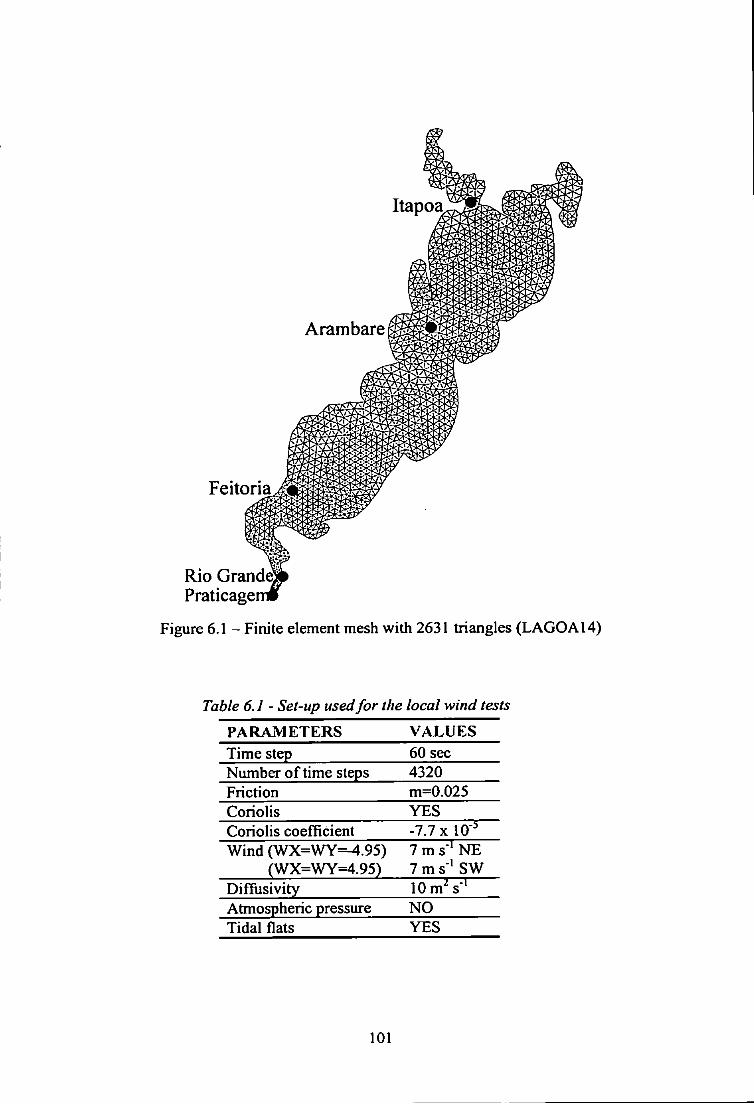
Arambare
Feitoria
Rio Grande. Praticage
Figure 6.1 - Finite element mesh with 2631 triangles (LAG0A14)
Table 6.1 - Set-up used for the local wind tests PARAMETERS VALUES Time step 60 sec Number of time steps 4320 Friction m=0.025 Coriolis YES Coriolis coefficient -7.7 X 10" Wind (WX=WY=-4.95) 7 m s'* NE
(WX=WY=4.95) 7 m s'* SW Diffusivity 10 m' S-'
Atmospheric pressure NO Tidal flats YES
101
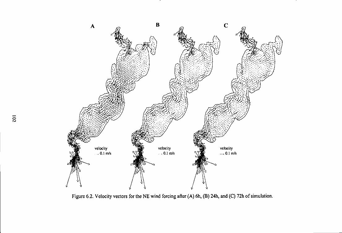
B
mmm.
s
velocity 0.1 m/s
velocity 0.1 m/s
velocity 0.1 m/s
Figure 6.2. Velocity vectors for the NE wind forcing after (A) 6h, (B) 24h, and (C) 72h of simulation.
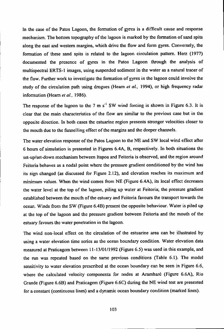
hi the case of the Patos Lagoon, the formation of gyres is a difficult cause and response
mechanism. The bottom topography of the lagoon is marked by the formation of sand spits
along the east and western margins, which drive the flow and form gyres. Conversely, the
formation of these sand spits is related to the lagoon circulation pattern, Herz (1977)
documented the presence of gyres in the Patos Lagoon through the analysis of
multispectral ERTS-1 images, using suspended sediment in the water as a natural tracer of
the flow. Further work to investigate the formation of gyres in the lagoon could involve the
study of the circulation path using drogues (Heam et al, 1994), or high frequency radar
infomiation (Heam a/., 1986).
The response of the lagoon to the 7 m s"' SW wind forcing is shown in Figure 6.3. It is
clear that the main characteristics of the flow are similar to the previous case but in the
opposite direction. In both cases the estuarine region presents stronger velocities closer to
the mouth due to the funnelling effect of the margins and the deeper channels.
The water elevation response of the Patos Lagoon to the NE and SW local wind effect after
6 hours of simulation is presented in Figures 6.4A, B, respectively. In both situations the
set-up/set-down mechanism between Itapoa and Feitoria is observed, and the region around
Feitoria behaves as a nodal point where the pressure gradient conditioned by the wind has
its sign changed (as discussed for Figure 2.12), and elevation reaches its maximum and
minimum values. When the wind comes from NE (Figure 6.4A), its local effect decreases
the water level at the top of the lagoon, piling up water at Feitoria; the pressure gradient
established between the mouth of the estuary and Feitoria favours the transport towards the
ocean. Winds from the SW (Figure 6.4B) present the opposite behaviour. Water is piled up
at the top of the lagoon and the pressure gradient between Feitoria and the mouth of the
estuary favours the water penetration in the lagoon.
The wind non-local effect on the circulation of the estuarine area can be illustrated by
using a water elevation time series as the ocean boundary condition. Water elevation data
measured at Praticagem between 11-13/01/1992 (Figure 6.5) was used in this example, and
the run was repeated based on the same previous conditions (Table 6.1). The model
sensitivity to water elevation prescribed at the ocean boundary can be seen in Figure 6.6,
where the calculated velocity components for nodes at Arambare (Figure 6.6A), Rio
Grande (Figure 6.6B) and Praticagem (Figure 6.6C) during the NE wind test are presented
for a constant (continuous lines) and a dynamic ocean boundary condition (marked lines).
103
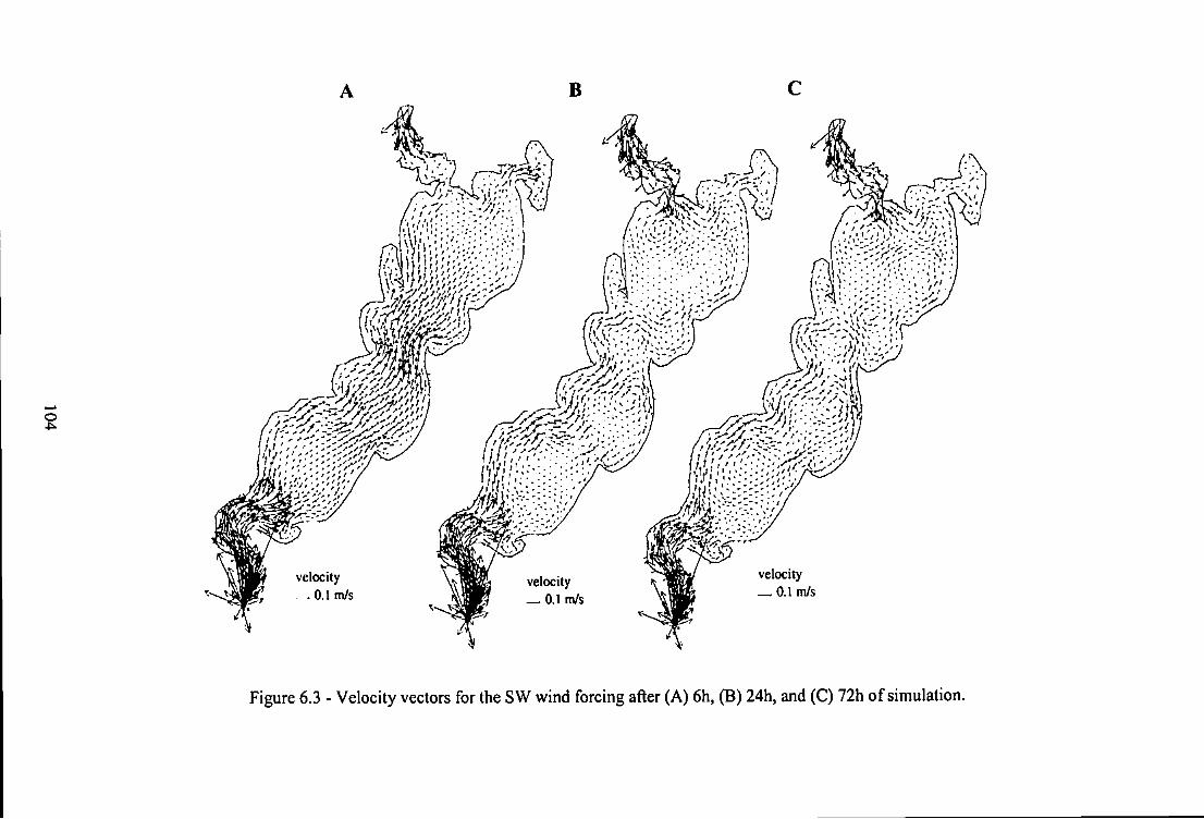
o 4
velocuy velocity — 0.1 m/s ,0.1m/s
velocity — 0.1 m/s
Figure 6.3 - Velocity vectors for the SW wind forcing after (A) 6h, (B) 24h, and (C) 72h of simulation.
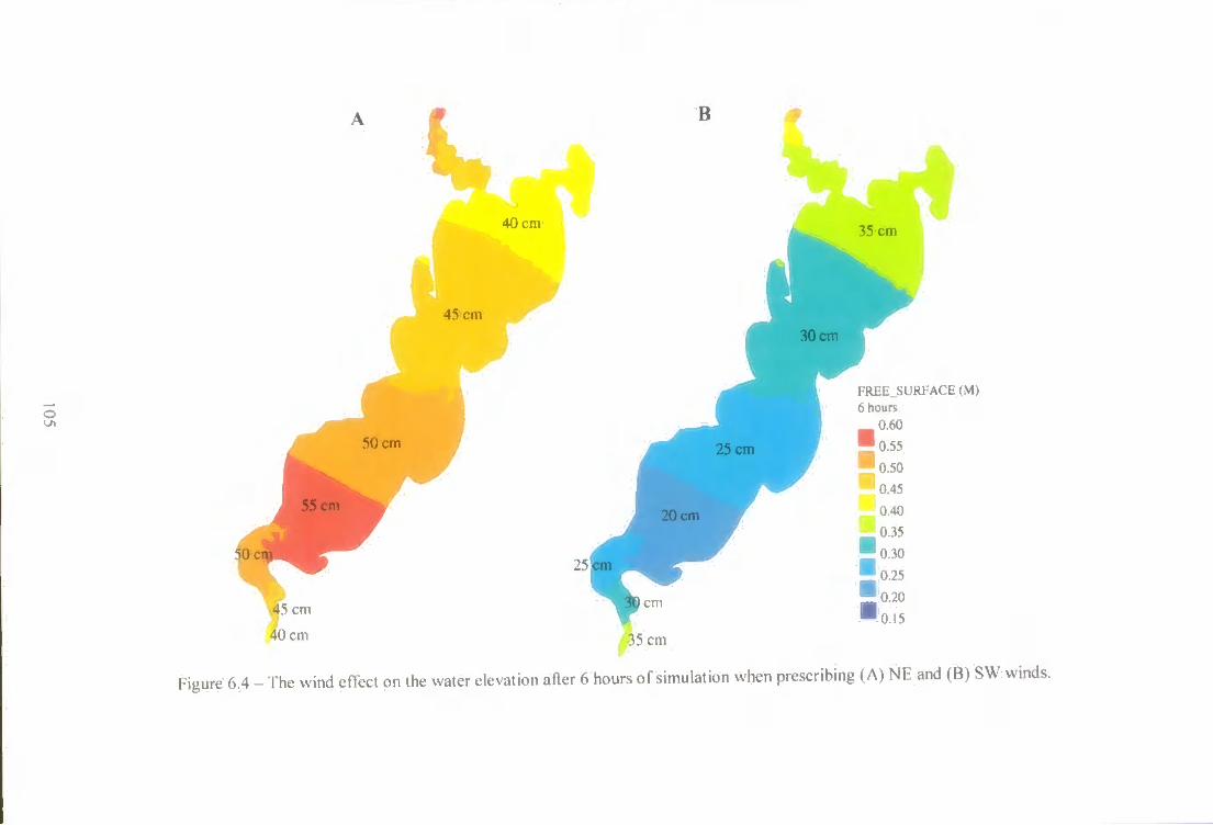
o
40 cm
45 cm
50 cm
cm
35 cm
l-Rlili SlIRl ACli (M) 6 hours
Figure 6.4 - Ihe wind effect on the water elevation aBer 6 hours of simulation when prescribing (A) NE and (B) SW winds.
0.6 - I
^ 0.4
a 0.2 -
0 6 12 18 24 30 36 42 48 54 60 66 72
Time (h) Figure 6.5 - Water elevation data from Praticagem (11-13/01/1992) used as dynamic ocean
boundary condition.
Results indicate that when using a constant water elevation boundary condition the system
takes around 10 hours to adjust, and achieves a steady state condition after 24 hours of
simulation. The use of a dynamic boundary condition does not afTect the water elevation
inside the lagoon (Figure 6.6A), but it is clearly modulating the water elevation on the
estuarine area (Figure 6.6B, C), where the steady state conditions disappears.
6.3. The Patos Lagoon response time to wind forcing
The Patos Lagoon response time to variations on the wind direction was further
investigated by applying the TELEMAC-2D model based on a finite element mesh with
2708 triangles. An imposed flow rate of 2000 m^ s"* was applied as the upstream boundary
condition and a constant elevation of the water surface was prescribed at the ocean
boundary. The NE wind was initially used to force the model during a three-day
simulation. Results from this test were then used as initial conditions for further three-day
simulations individually prescribing wind from different directions (SW, S, E) in order to
assess the lagoon response time to different winds. The same procedure was repeated when
starting the simulation with a SW wind and then varying to NE, S, and E (Table 6.2).
106
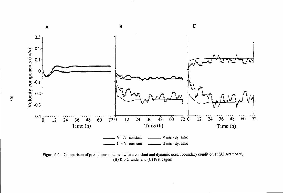
B
o S -0.2
^ -0.31
12 24 36 48 60 72 0 12 24 36 48 60 72 0 12 24 36 48 60 72 Time (h) Time (h) Time (h)
V m/s - constant U m/s - constant *.
V m/s - dynamic U m/s - dynamic
Figure 6.6 - Comparison of predictions obtained with a constant and dynamic ocean boundary condition at (A) Arambar6, (B) Rio Grande, and (C) Praticagem
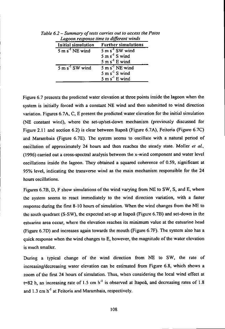
Table 6.2- Summary of tests carries out to access the Patos Lagoon response time to different winds
Initial simulation Further simulations 5 m s"* NE wind 5 m s'' SW wind
5 m s"* S wind 5 m s'* E wind
5 m s"' SW wind 5 m s" NE wind 5 m s"* S wind 5 m s'* E wind
Figure 6.7 presents the predicted water elevation at three points inside the lagoon when the
system is initially forced with a constant NE wind and then submitted to wind direction
variation. Figures 6.7A, C, E present the predicted water elevation for the initial simulation
(NE constant wind), where the set-up/set-down mechanism (previously discussed for
Figure 2.11 and section 6.2) is clear between Itapoa (Figure 6.7A), Feitoria (Figure 6.7C)
and Marambaia (Figure 6.7E). The system seems to oscillate with a natural period of
oscillation of approximately 24 hours and then reaches the steady state. MoUer et al,
(1996) carried out a cross-spectral analysis between the x-wind component and water level
oscillations inside the lagoon. They obtained a squared coherence of 0.59, significant at
95% level, indicating the transverse wind as the main mechanism responsible for the 24
hours oscillations.
Figures 6.7B, D, F show simulations of the wind varying from NE to SW, S, and E, where
the system seems to react immediately to the wind direction variation, with a faster
response during the first 8-10 hours of simulation. When the wind changes from the NE to
the south quadrant (S-SW), the expected set-up at Itapoa (Figure 6.7B) and set-down in the
estuarine area occur, where the elevation reaches its minimum value at the estuarine head
(Figure 6.7D) and increases again towards the mouth (Figure 6.7F). The system also has a
quick response when the wind changes to E, however, the magnitude of the water elevation
is much smaller.
During a typical change of the wind direction from NE to SW, the rate of
increasing/decreasing water elevation can be estimated from Figure 6.8, which shows a
zoom of the first 24 hours of simulation. Thus, when considering the local wind effect at
t=82 h, an increasing rate of 1,5 cm h"* is observed at Ilapoa, and decreasing rates of 1.8
and 1.3 cm h ' at Feitoria and Marambaia, respectively.
108
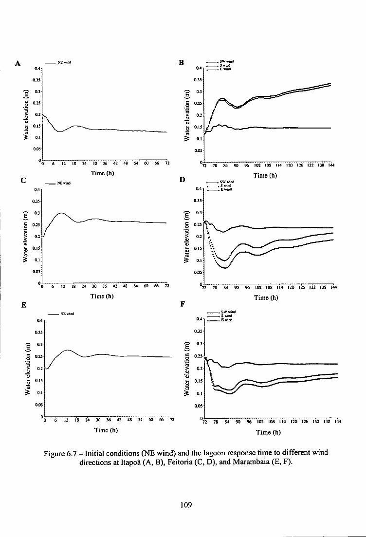
A — SWwiad SwiDd Ewiad
24 30 36 42 48
Time (h)
60 66 72
6 12 18 24 30 36 42 48
Time (h)
54 60 66 72
D
72 78 84 90 96 102 108 114 IM 126 132 138 144
Time (h)
a4
0J5
0.3
0.2
0.15
0.1
0.05
0
SW»ind ,S wind .EwiDd
72 78 84 90 96 102 108 114 120 126 132 138 144
Time (h)
0.4
0J5
0.3
0.25
0.2
0.15
0.1
0.05
0 6 12 18 24 30 36 42 48 54 60 66 72
Time (h)
I I
SWwind S wind Ewiod
72 78 90 96 102 108 114 120 126 132 138 144
Time (h)
Figure 6.7 - Initial conditions (NE wind) and the lagoon response time to different wind directions at Itapoa (A, B), Feitoria (C, D), and Marambaia (E, F).
109
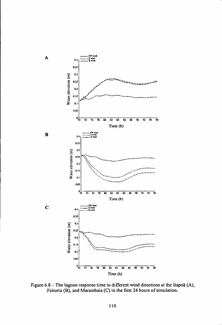
B
0.4
0J5
0.3
ion
{
0.25
> 0.2 U
CIS u
0.1
0.05
0.
SWwiod -.Swind _ Bwind
72 74 76 78 SO 82 84 8
Time (h)
90 92 94 96
0.4
0.33
a3
ion
(
0.25
> 0.2 U L . 0.15 CJ 0.15 B
0.1
0.05
°7
SWwind
72 74 76 78 SO 82 84 S6
Time (h)
90 92 94 96
0.4
0.35
a3
ion
(
0.25
> 0.2 u u 0.15
0.1
0.05
.SWwind ,S»Tnd , Ewind
72 74 76 78 80 82 84 8
Time (h)
90 92 94 96
Figure 6.8 - The lagoon response time to different wind directions at the Itapoa (A), Feitoria (B), and Marambaia (C) in the first 24 hours of simulation.
110
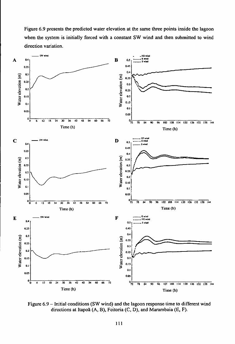
Figure 6.9 presents the predicted water elevation at the same three points inside the lagoon
when the system is initially forced with a constant SW wind and then submitted to wind
direction variation.
. NEwtmJ
Swiad
0.2
0.1
24 30 36 42 48
Time (h) 90 96 102 lOS 114 120 126 132 138 144
Time (h)
24 30 36 42
Time (h) 60 66 72
E — a4
0J5
0.3
0.25
a2
O.IS
0.1
0.05
0
72 78 S4 90 96 102 108 114 120 126 132 138
Time (h)
F — Ewintl NEwind
12 18 24 30 36 42 48
Time (h)
60 66 72
0.5
0.45
0.4
0.35 c o 0.3
> 0.25 _o o 0.2 o
> O.IS
> 0.1
0.05
0 72 78 84 90 96 102 108 114 120 126 132 138 144
Time (h)
Figure 6.9 - Initial conditions (SW wind) and the lagoon response time to different wind directions at Itapoa (A, B), Feitoria (C, D), and Marambaia (E, F).
I l l
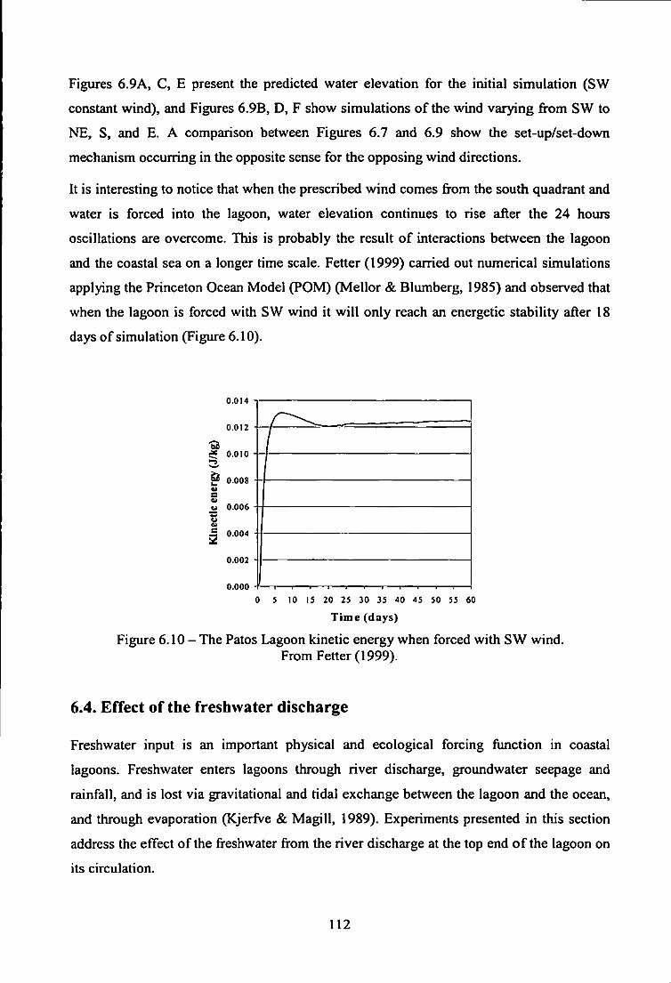
Figures 6.9A, C, E present the predicted water elevation for the initial simulation (SW
constant wind), and Figures 6.9B, D, F show simulations of the wind varying from SW to
NE, S, and E. A comparison between Figures 6.7 and 6.9 show the set-up/set-down
mechanism occurring in the opposite sense for the opposing wind directions.
It is interesting to notice that when the prescribed wind comes from the south quadrant and
water is forced into the lagoon, water elevation continues to rise after the 24 hours
oscillations are overcome. This is probably the result of interactions between the lagoon
and the coastal sea on a longer time scale. Fetter (1999) carried out numerical simulations
applying the Princeton Ocean Model (POM) (Mellor & Blumberg, 1985) and observed that
when the lagoon is forced with SW wind it will only reach an energetic stability after 18
days of simulation (Figure 6.10).
0.014
0.012
-SB 0.010
^ 0.008
s u 0.006
i
I 0.004
0.002
0.000
T I I 1 1 1
0 5 10 15 20 25 30 35 40 45 50 55 60
Time (days)
Figure 6.10 - The Patos Lagoon kinetic energy when forced with SW wind. From Fetter (1999).
6.4. Effect of the freshwater discharge
Freshwater input is an important physical and ecological forcing function in coastal
lagoons. Freshwater enters lagoons through river discharge, groundwater seepage and
rainfall, and is lost via gravitational and tidal exchange between the lagoon and the ocean,
and through evaporation (Kjerfve & Magill, 1989). Experiments presented in this section
address the effect of the freshwater from the river discharge at the top end of the lagoon on
its circulation.
112
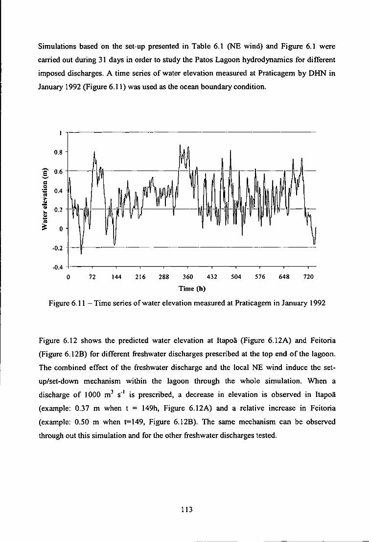
Simulations based on the set-up presented in Table 6.1 (NE wind) and Figure 6.1 were
carried out during 31 days in order to study the Patos Lagoon hydrodynamics for different
imposed discharges. A time series of water elevation measured at Praticagem by DHN in
January 1992 (Figure 6.11) was used as the ocean boundary condition.
1 1
0.8 H
'E 0.6
>
0.2 H
-0.2
-0.4 1 1 1 1 1 1 1 1 1 1 —
0 72 144 216 288 360 432 504 576 648 720
Time (h)
Figure 6.11 - Time series of water elevation measured at Praticagem in January 1992
Figure 6.12 shows the predicted water elevation at Itapoa (Figure 6.12A) and Feitoria
(Figure 6.12B) for different freshwater discharges prescribed at the top end of the lagoon.
The combined effect of the freshwater discharge and the local NE wind induce the set
up/set-down mechanism within the lagoon through the whole simulation. When a
discharge of 1000 m^ s"' is prescribed, a decrease in elevation is observed in Itapoa
(example: 0.37 m when t = 149h, Figure 6.12A) and a relative increase in Feitoria
(example: 0.50 m when t=149, Figure 6.12B). The same mechanism can be observed
through out this simulation and for the other freshwater discharges tested.
113
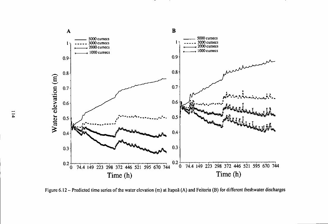
B SOOOcumecs
l l 3000cumecs 2000cumecs lOOOcumecs
5000 cumecs 3000 cumecs 2000 cumecs
« lOOOcumecs
S 0.5
, 0.2 6 74.4 149 223 298 372 446 521 595 670 744 ' "0 74.4 149 223 298 372 446 521 595 670 744
•| ' T ' T I I I
Time (h) Time (h)
Figure 6.12 - Predicted time series of the water elevation (m) at ItapoS (A) and Feitoria (B) for different freshwater discharges
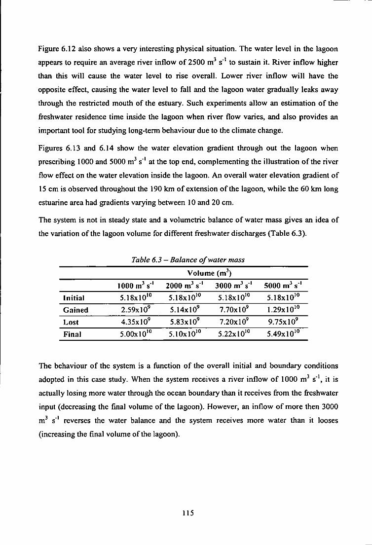
Figure 6.12 also shows a very interesting physical situation. The water level in the lagoon
appears to require an average river inflow of 2500 m" s"* to sustain it. River inflow higher
than this will cause the water level to rise overall. Lower river inflow v^U have the
opposite effect, causing the water level to fall and the lagoon water gradually leaks away
through the restricted mouth of the estuary. Such experiments allow an estimation of the
freshwater residence time inside the lagoon when river flow varies, and also provides an
important tool for studying long-term behaviour due to the climate change.
Figures 6.13 and 6.14 show the water elevation gradient through out the lagoon when
prescribing 1000 and 5000 m^ s * at the top end, complementing the illustration of the river
flow effect on the water elevation inside the lagoon. An overall water elevation gradient of
15 cm is observed throughout the 190 km of extension of the lagoon, while the 60 km long
estuarine area had gradients varying between 10 and 20 cm.
The system is not in steady state and a volumetric balance of water mass gives an idea of
the variation of the lagoon volume for different freshwater discharges (Table 6.3).
Table 6.3- Balance of water mass
Volume (m"*) 1000 m^ s"* 2000 s"' 3000 m^ s ' 5000 s *
Initial 5.18x10*° 5.18x10*° 5.18x10*° 5.18x10*° Gained 2.59x10^ 5.14x10^ 7.70x10^ 1.29x10*° Lost 4.35x10^ 5.83x10^ 7.20x10^ 9.75x10^ Final 5.00x10*° 5.10x10*° 5.22x10*° 5.49x10*°
The behaviour of the system is a ftmction of the overall initial and boundary conditions
adopted in this case study. When the system receives a river inflow of 1000 m"' s"*, it is
actually losing more water through the ocean boundary than it receives from the freshwater
input (decreasing the final volume of the lagoon). However, an inflow of more then 3000
m^ s'* reverses the water balance and the system receives more water than it looses
(increasing the final volume of the lagoon).
115
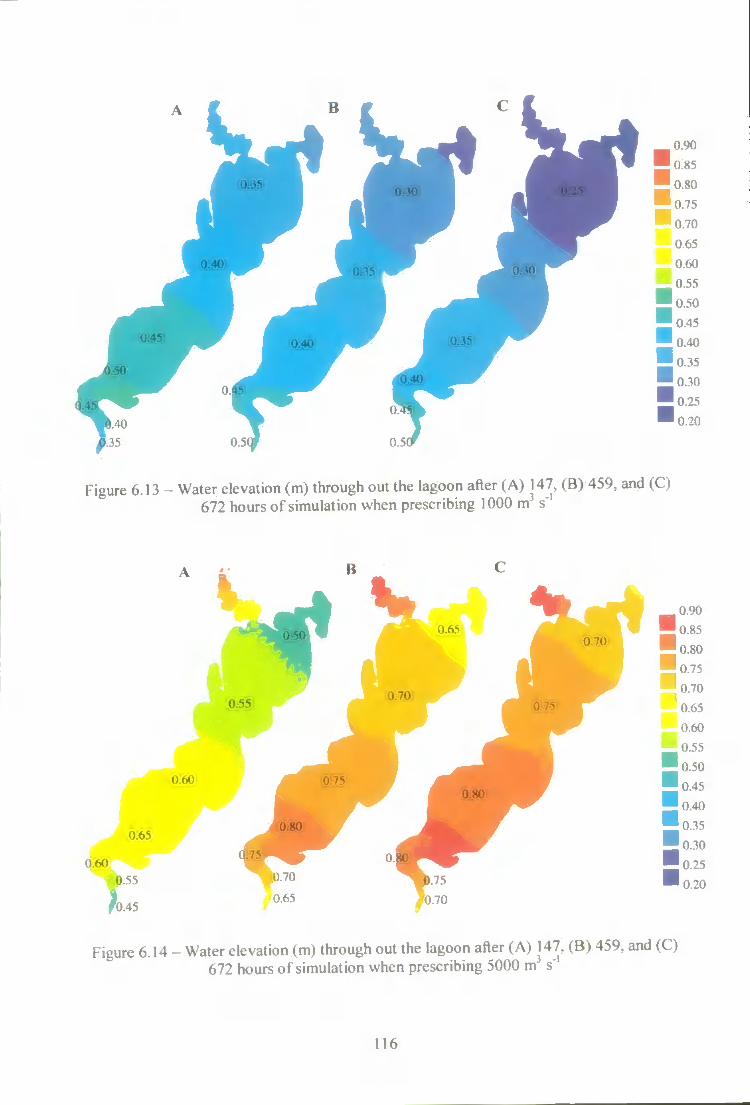
0.90 0.85 0.80 0.75 0.70 0.65 0.60 0.55 0.50 0.45 0.40 0.35 0.. 0
I 0.20
Figure 6.13 - Water elevation (m) through out the lagoon after ( A) 147, (B) 459, and (C) 672 hours of simulation when prescribing 1000 m s
0.f)0
0.65
0.60
0.45
0.90 0.85 0.80 0.75 0.70 0.65 0.60 0..S5 0.50 0.45 0.40
0.30 0.25
I 0.20
Figure 6.14 - Water elevation (m) through out the lagoon after (A) 147. (B) 459, and (C) 672 hours of simulation w hen prescribing 5000 m s"
116
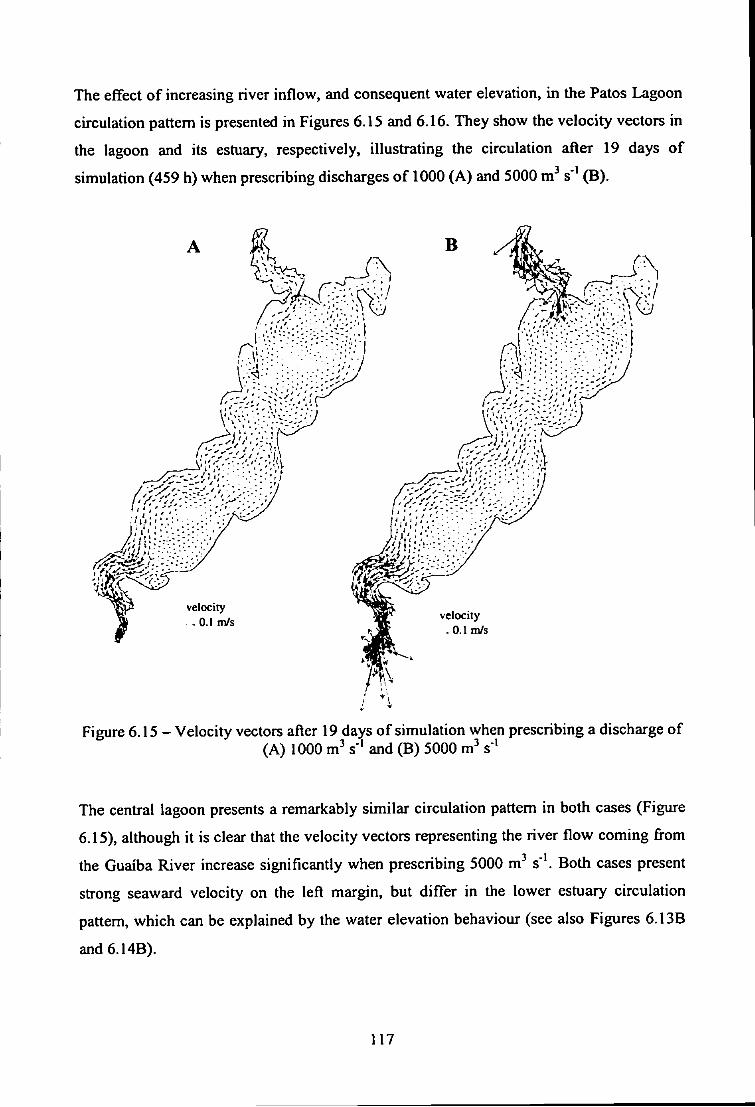
The effect of increasing river inflow, and consequent water elevation, in the Patos Lagoon
circulation pattern is presented in Figures 6.15 and 6.16. They show the velocity vectors in
the lagoon and its estuary, respectively, illustrating the circulation after 19 days of
simulation (459 h) when prescribing discharges of 1000 (A) and 5000 m^ s"' (B).
velocity . 0.1 m/s velocity
. 0.1 nVs
> * . • - I As
Figure 6.15 - Velocity vectors after 19 days of simulation when prescribing a discharge of (A) 1000 m^ s * and (B) 5000 s 3 .-1
The central lagoon presents a remarkably similar circulation pattern in both cases (Figure
6.15), although it is clear that the velocity vectors representing the river flow coming from
the Guaiba River increase significantly when prescribing 5000 m^ s *. Both cases present
strong seaward velocity on the left margin, but differ in the lower estuary circulation
pattern, which can be explained by the water elevation behaviour (see also Figures 6.13B
and 6. MB).
117
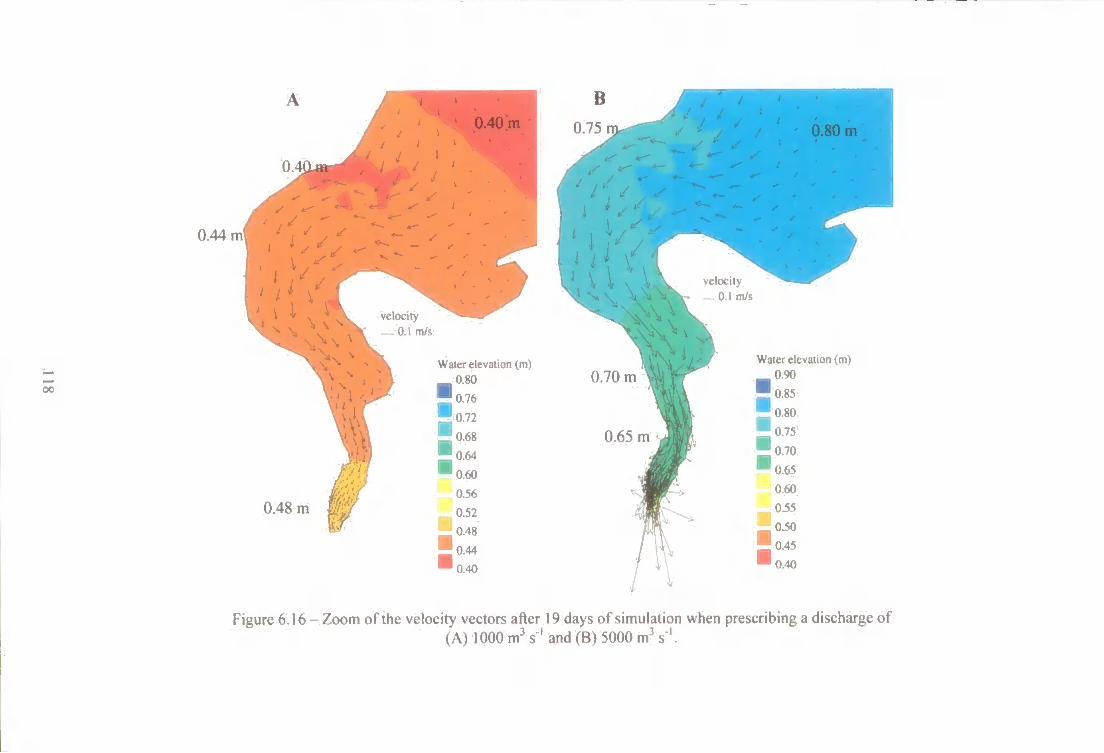
0.44 m
0.1 m/s
velocity 0.1 m/5
Water elcvalion (m) Water elevation (m) 0.70 m
0.65 m
0.48 m
Figure 6.16 - Zoom of the velocity vectors after 19 days of simulation when prescribing a discharge of (A) 1000 m^ s*' and (B) 5000 m^ s"'.
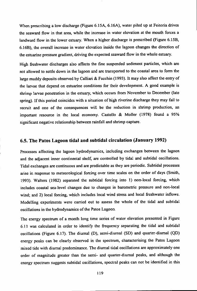
When prescribing a low discharge (Figure 6.15A, 6.16A), water piled up at Feitoria drives
the seaward flow in that area, while the increase in water elevation at the mouth forces a
landward flow in the lower estuary. When a higher discharge is prescribed (Figure 6.15B,
6.16B), the overall increase in water elevation inside the lagoon changes the direction of
the estuarine pressure gradient, driving the expected seaward flow in the whole estuary.
High freshwater discharges also affects the fine suspended sediment particles, which are
not allowed to settle down in the lagoon and are transported to the coastal area to form the
large muddy deposits observed by Calliari & Facchin (1993). It may also affect the entry of
the larvae that depend on estuarine conditions for their development. A good example is
shrimp larvae penetration in the estuary, which occurs from November to December (late
spring). If this period coincides with a situation of high riverine discharge they may fail to
recruit and one of the consequences will be the reduction in shrimp production, an
important resource in the local economy, Castello & Moller (1978) found a 95%
significant negative relationship between rainfall and shrimp capture.
6.5. The Patos Lagoon tidal and subtidal circulation (January 1992)
Processes affecting the lagoon hydrodynamics, including exchanges between the lagoon
and the adjacent inner continental shelf, are controlled by tidal and subtidal oscillations.
Tidal exchanges are continuous and are predictable as they are periodic. Subtidal processes
arise in response to meteorological forcing over time scales on the order of days (Smith,
1993). Walters (1982) separated the subtidal forcing into 1) non-local forcing, which
includes coastal sea-level changes due to changes in barometric pressure and non-local
wind; and 2) local forcing, which includes local wind stress and local freshwater inflows.
Modelling experiments were carried out to assess the whole of the tidal and subtidal
oscillations in the hydrodynamics of the Patos Lagoon.
The energy spectrum of a month long time series of water elevation presented in Figure
6.11 was calculated in order to identify the frequency separating the tidal and subtidal
oscillations (Figure 6.17). The diumal (D), semi-diurnal (SD) and quarter-diurnal (QD)
energy peaks can be clearly observed in the spectrum, characterising the Patos Lagoon
mixed tide with diumal predominance. The diumal tidal oscillations are approximately one
order of magnitude greater than the semi- and quarter-diurnal peaks, and although the
energy spectrum suggests subtidal oscillations, spectral peaks can not be identified in this
119
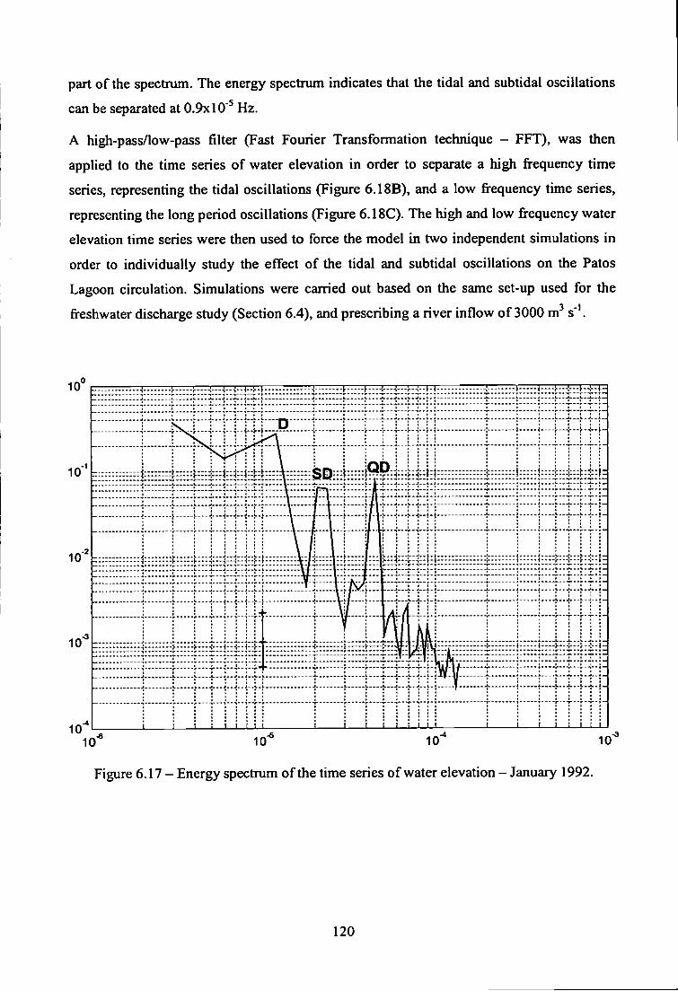
part of the spectrum. The energy spectrum indicates that the tidal and subtidal oscillations
can be separated at 0.9x10' Hz.
A high-pass/low-pass filter (Fast Fourier Transformation technique - FFT), was then
applied to the time series of water elevation in order to separate a high frequency time
series, representing the tidal oscillations (Figure 6.18B), and a low frequency time series,
representing the long period oscillations (Figure 6.18C). The high and low frequency water
elevation time series were then used to force the model in two independent simulations in
order to individually study the effect of the tidal and subtidal oscillations on the Patos
Lagoon circulation. Simulations were carried out based on the same set-up used for the
freshwater discharge study (Section 6.4), and prescribing a river inflow of 3000 m^ s '.
Figure 6.17 - Energy spectrum of the time series of water elevation - January 1992.
120
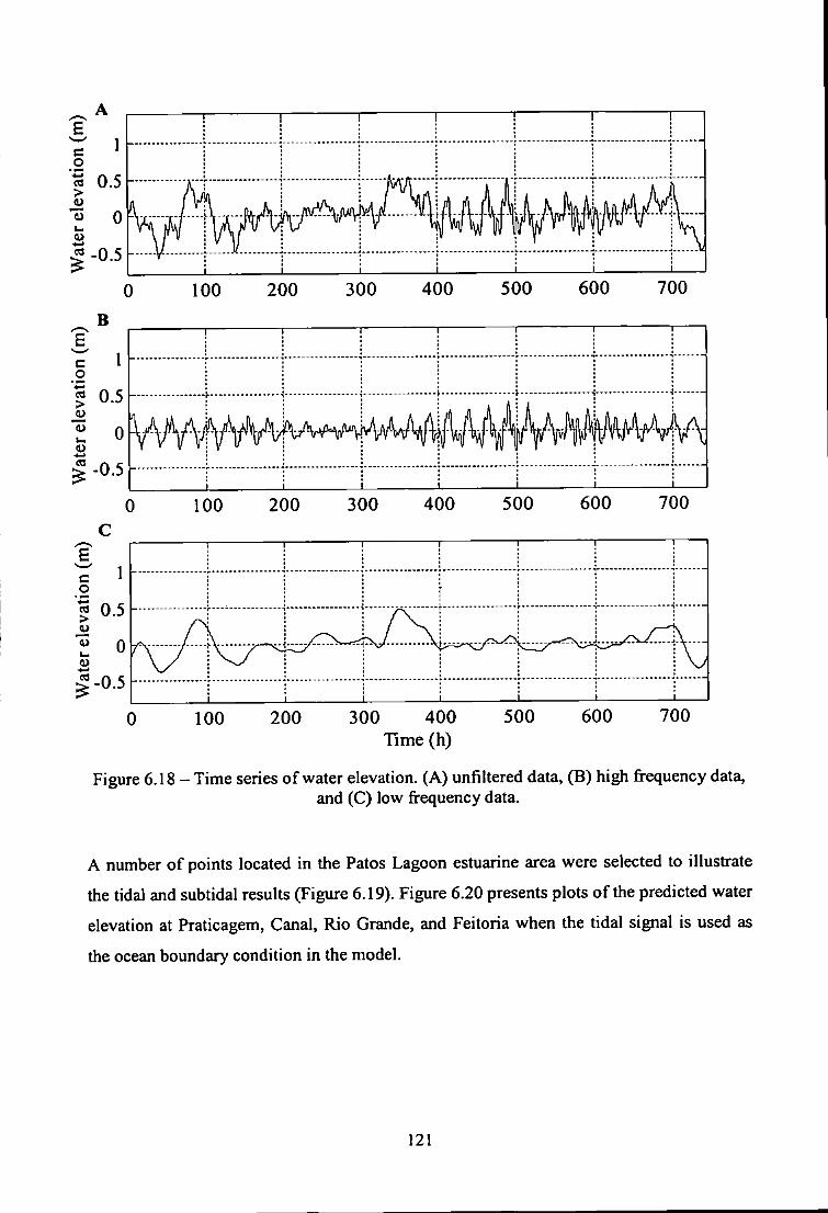
B
c 1 o > 0.5
Urn 0 B
-0.5
c 1 o
'•1—' CO 0.5 >
0.5
0
-0.5
0 100 200 300 400 Time (h)
500 600 700
Figure 6.18 - Time series of water elevation. (A) unfiltered data. (B) high frequency data, and (C) low frequency data.
A number of points located in the Patos Lagoon estuarine area were selected to illustrate
the tidal and subtidal results (Figure 6.19). Figure 6.20 presents plots of the predicted water
elevation at Praticagem, Canal, Rio Grande, and Feitoria when the tidal signal is used as
the ocean boundary condition in the model.
121
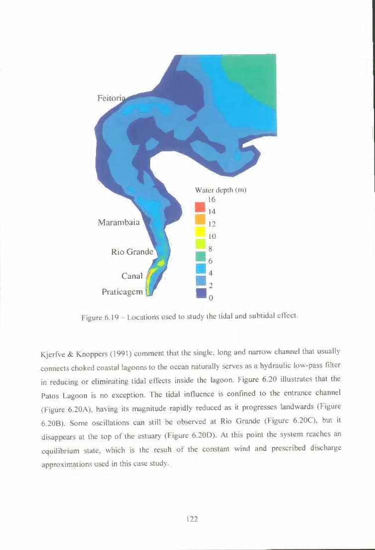
Feitori
Water depth (m) 16
Marambaia
Rio Grande
Canal
Pralicagcm
Figure 6.19 - Locations used to .study the tidal and subtidal etTect.
Kjerfve & Knoppers (1991) comment that the single, long and narrow channel that usually
connects choked coastal lagoons to the ocean naturally serves as a hydraulic low-pass filter
in reducing or eliminating tidal effects inside the lagoon. Figure 6.20 illustrates that the
Patos Lagoon is no exception. The tidal influence is confined to the entrance channel
(Figure 6.20A), having its magnitude rapidly reduced as it progresses landwards (Figure
6.20B). Some oscillations can still be observed at Rio Grande (Figure 6.20C), but it
disappears at the top of the estuary (Figure 6.20D). At this point the system reaches an
equilibrium state, which is the resuh of the constant wind and prescribed discharge
approximations used in this case study.
122
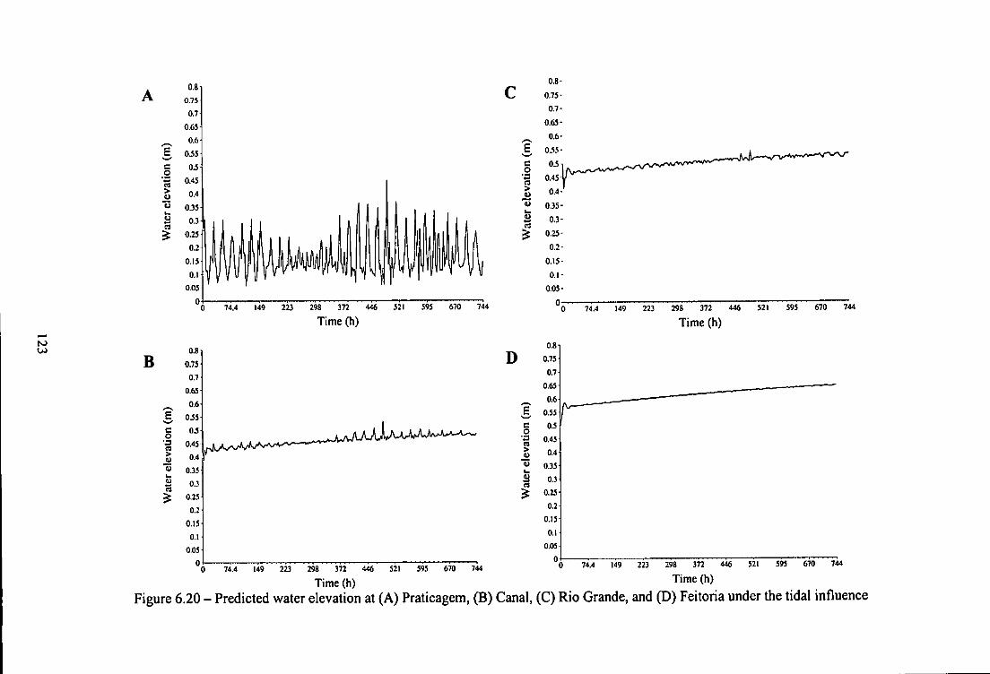
to B
0.8
0.75
0.7
0.63
0.6
s 0.55
c OS o
OS
0.45 C3
0.45 > O 0.4 u 0J5 t. u 0.3
0.25-
0.2
0.15
0.1
0.05
0 {
0.8
0.73
0.7
0.63
0.6
E 0J5
c OJ o
OJ
•3 0.45 0.45
> 0.4
I j 0.35 u u 0.3
0.25
0.2
0.15
0.1
0.03
0
(
74.4 223 298 372 446
Time (h) 744
74.4 149 223 298 372
Time (h) 446 521 595 670 744
D
0.8
0.75
0.7
0.63
0.6
0.55
OS
0.45
0.4
0J5
0.3
0.25
0.2
0.15
0.1
0.05
0
0,8'
0.75
0.7
0.63
0.6
0.55
0.5
0.43
0.4
0.33
0.3
0.25
0.2
0.13
0.1
0.05
0
74.4 149 223 298 372
Time (h) 446 521 595 670 744
74.4 149 223 298 372
Time (h) 446 521 393 670 744
Figure 6.20 - Predicted water elevation at (A) Praticagem, (B) Canal, (C) Rio Grande, and (D) Feitoria under the tidal influence
Moller et al. (2001) commented that the subtidal dynamics of the Patos Lagoon can be
divided in two distinct periods. During most of the year the circulation is wind driven due
to low to moderate river discharge, while the during the annual flood peak in late winter,
the riverine input plays the main role. However, the available data set for January 1992 is
limited, and the set-up used for the subtidal experiments is based on a constant wind and
freshwater discharge. Thus, the long-period oscillations considered here are limited to the
non-local effect, represented by the water elevation at the ocean boundary.
Figure 6.21 presents plots of the predicted water elevation at Praticagem, Canal, Rio
Grande, and Feitoria when the long period oscillations are used as the ocean boundary
condition in the model. Figure 6.21 A shows the strong filtering effect of the channel for
the long period oscillations. Strong peaks of water elevation are still observed at Canal
(Figure 6.21B) and Rio Grande (Figure 6.21C), but are reduced moving landwards (Figure
6.2ID), although a small peak is still observed at Feitoria after approximately 350 hours.
An example of the circulation of the Patos Lagoon after 15 days (360 hours) of simulation,
when the system is individually forced with the tidal and subtidal oscillations, is presented
in Figure 6.22. The predicted velocity vectors indicate a similar picture in both cases, with
a seaward flow on the left margin and some gyres in the northern cell of the lagoon.
However, the prediction of the water elevation indicates that the perturbation caused by the
long period oscillations penetrates further than the tidal oscillation through the inlet (Figure
6.22B),
Figure 6.23 concentrates on the estuarine circulation and shows ebb flow dominating the
estuary in both cases, with velocity vectors evenly distributed until the Rio Grande area.
After Rio Grande, the direction of the velocity vectors varies due to the dynamics of the
area. A stronger hydrodynamics and outflow is observed for the tidal forcing case. This is
most likely to be related to the water elevation prescribed at t=360 hours (Figure 6.18), as
the pressure gradient established between Rio Grande and the mouth of the estuary during
the tidal experiment is stronger and forces more water out of the lagoon.
124
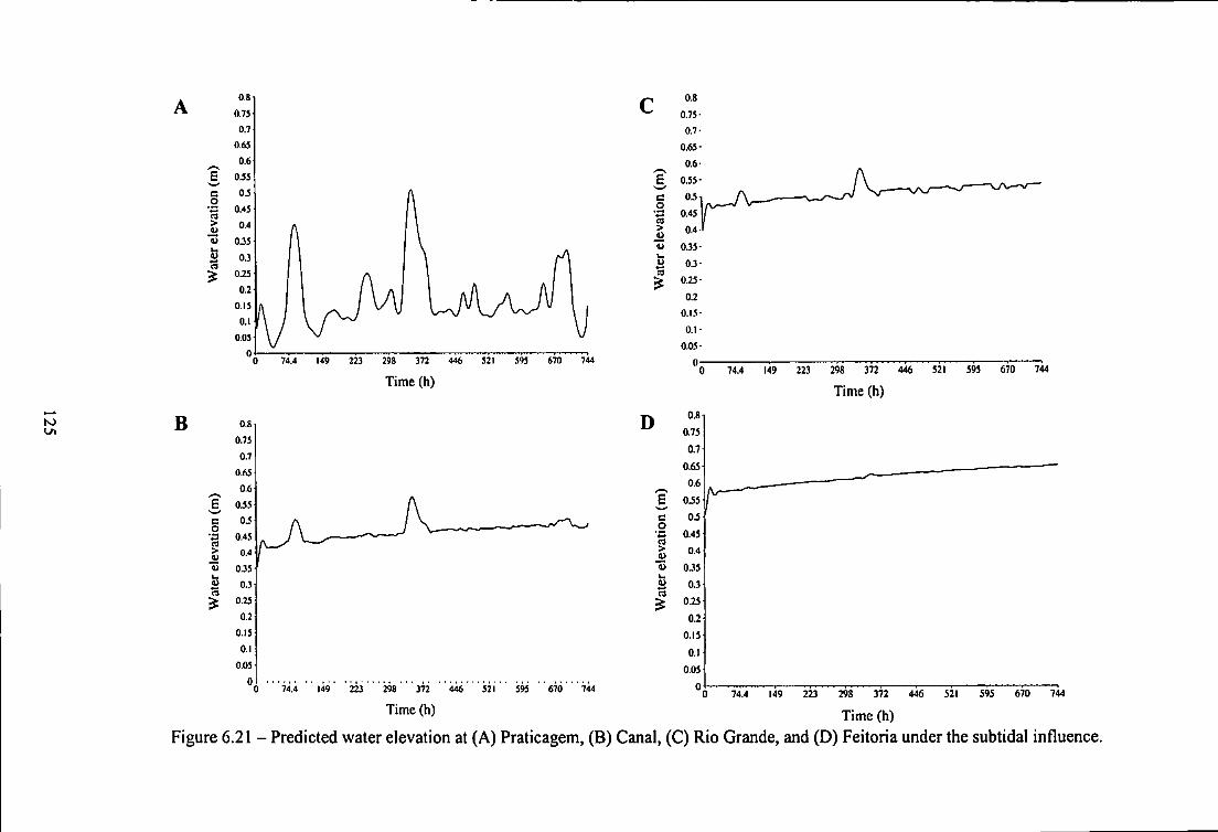
B 0.8
0.75
0.7
0.6S
0.6
OSS
c 0.5 o
0.45 a > 0.4
"u 0.33
0.3
0.25
0.2
0.15
0.1
0.05
0
Time (h)
D
0.8
0.75-
0.7-
0.65-
0.6-
0.55-
OJ
0.45
0.4
OM
OJ
0.25
0.2
0.15
0.1
0.05
0
74.4 149 223 298 372 446 521 595 670
0.8
0.75
0.7
0.65
0.6
? 055
c OJ o ' C 0.45 a > 0.4
"S 0.35 Urn u 0.3
0.25
0.2
0.15
0.1
0.05
0
74.4 149 223 298 372
Time (h)
446 521 595 670 744
74.4 446 521 595 670 744
Time (h) 149 223 298 372
Time (h)
Figure 6.21 - Predicted water elevation at (A) Praticagem, (B) Canal, (C) Rio Grande, and (D) Feitoria under the subtidal influence.
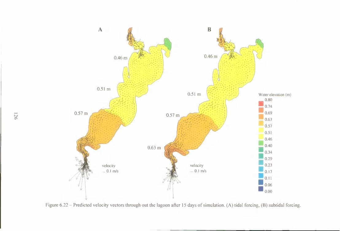
0.46 m
0.51 m
I J 0.57 m 0.57 m
0.46 m
0.51 m
0.63 m
velocity -0 .1 m/s
velocity - 0 . 1 m/s
Water elevation (m) 0.80
J 0.74
0.57
0.51
0.46
_ 0.40
'o.34 [o.29 • 0.23
J 0.17
J 0.11
jo.06 'o.oo
Figure 6.22 - Predicted velocity vectors through out the lagoon after 15 days of simulation. (A) tidal forcing, (B) subtidal forcing.
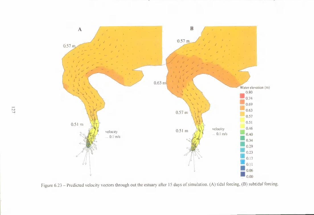
0.57 m.
0.51 m
velocity .0.1 m/s
0.57 m
0.63 m
0.57 m
0.51 m velocity 0.1 m/s
Water elevation (m) 0.80
0.74
0.69
0.63
0.57
0.51
0.46
0.40
0.34
0.29
0.23
0.17
O.ll 0.06
0.00
Figure 6.23 - Predicted velocity vectors through out the estuary after 15 days of simulation. (A) tidal forcing, (B) subtidal forcing.
Ideally, predictions from these simulations should be able to assess the whole of the tidal
and subtidal oscillations in the hydrodynamics o f the Patos Lagoon. However, the time
series of water elevation from January 1992 is only representative of the summer months,
when the freshwater discharge is low to moderate and the weather fronts over the region
are not so intense. For such conditions, predicted results indicate that the tidal and subtidal
oscillation have similar magnitudes during the studied period. This picture is expected to
change during the winter months, when the area is marked by the passage o f much stronger
weather fronts and the subtidal oscillations combined with the riverine input from the north
of the lagoon are expected to overcome the tidal effect.
6.5.1. Tidal and subtidal attenuation
Results also indicate that the entrance channel not only filters the astronomical tides but
also attenuates the long period oscillations generated offshore. Moller et al. (1996) point
out the attenuation of these oscillations throughout the channel, although a coefficient
describing the tidal and subtidal attenuation was not calculated. Ippen & Harleman (1961)
developed a method which relates the relative times of high water along the estuary, the
tidal amplitudes, and the phase change to a damping coefficient which specifies the change
in amplitude with distance along the estuary caused by fiiction. Such method would be
appropriate for estimating the tidal attenuation in the Patos Lagoon estuary i f a more
comprehensive data set was available.
Another option to estimate the tidal and subtidal attenuation is to shift firom the time
domain into the frequency domain applying a cross-spectral analysis, which results in a co-
spectrum (spectral density function), a coherence spectrum and a phase spectrum (Russell,
1990). This method was chosen because the co-spectrum is a useftil function for estimating
the contribution of the predicted water elevation time series at different frequencies and
because the attenuation of the tidal and subtidal signals throughout the estuary can be
estimated by the spectral density function.
A cross-power spectrum defines the relationship between two variables. I f these variables
are completely independent the co-spectrum is zero, and i f they are identical it becomes the
ordinary power spectrum. The derived coherence between the two times series is a measure
of how well correlated the two sequences are as a function of frequency, being equal to 1 i f
one signal is a constant times the other (Butt, 1999). The coherence spectrum has a
confidence limit, which is the limit below what the coherence values can occur by chance.
Therefore, for frequencies at which the coherence is below this limit, any co-spectral
128
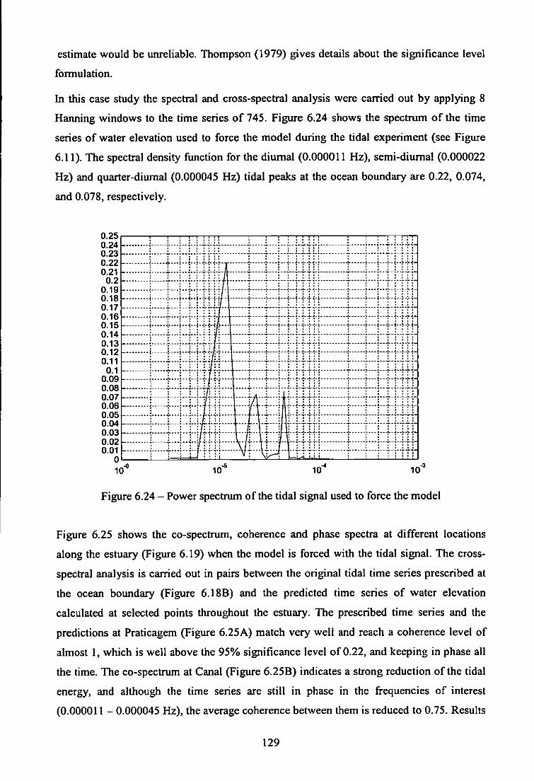
estimate would be unreliable. Thompson (1979) gives details about the significance level
formulation.
In this case study the spectral and cross-spectral analysis were carried out by applying 8
Manning windows to the time series of 745. Figure 6.24 shows the spectrum of the time
series of water elevation used to force the model during the tidal experiment (see Figure
6.11). The spectral density function for the diurnal (0.000011 Hz), semi-diurnal (0.000022
Hz) and quarter-diumal (0.000045 Hz) tidal peaks at the ocean boundary are 0.22, 0.074,
and 0.078, respectively.
0.25 0.24 0.23 0.22 0.21
0.2 0.19 0.18 0.17 0.16 0.15 0.14 0.13 0.12 0.11
0.1 0.09 0.08 0.07 0.06 0.05 0.04 0.03 0.02 0.01
0
J j I I I I I ! 1 1 1 1—T J ' J j ' [ [ ] ' j ] ^
! \ ' ! ! ! • ! ; : : ; : ; : 1 : : :
: : : : : : : ; ; : : :
: : ; : i : : ^ J i : : : : ; : : : : : : : : : :1 : '. : : : : : : -i——j— -:--y-i"H-: i f""i"i":"l"H" : ;
-i——j— -:--y-i"H-: i f""i"i":"l"H" - - • i < 1. . t h " ! -f H " i - - M - j -:- f""i""i'i"i"H"
• > • < « * • « > • * ! » « • • < I » l l l i a f t • t l l l « « t • • • • « * ! • • «
• • 11 1 • • t I • I 1 1 1 1 I 1 • < • 1 • • j[ • 1 I 1 1 • ( • • I I I !
: ; ; : : : ; : : : :
I ! ! ! ! ! ! ! ! I I ! ! 1 ! ! '
1 1 • • i t i t i 1 1
; \ : : ; : / ; : ;
r I ; : t : ; : ; •—\ ^
L I . . ! i j . J . J .
• —
i i-4-j--i-i":-— ^ - " i " A - • ij- A- -l- A- . . . . .
; ; — ! — ! — / • • !
10 10 10" 10'
Figure 6.24 - Power spectrum of the tidal signal used to force the model
Figure 6.25 shows the co-spectrum, coherence and phase spectra at different locations
along the estuary (Figure 6.19) when the model is forced with the tidal signal. The cross-
spectral analysis is carried out in pairs between the original tidal time series prescribed at
the ocean boundary (Figure 6.18B) and the predicted time series of water elevation
calculated at selected points throughout the estuary. The prescribed time series and the
predictions at Praticagem (Figure 6.25A) match very well and reach a coherence level of
almost 1, which is well above the 95% significance level of 0.22, and keeping in phase all
the time. The co-spectrum at Canal (Figure 6.25B) indicates a strong reduction of the tidal
energy, and although the time series are still in phase in the fi-equencies of interest
(0.000011 - 0.000045 Hz), the average coherence between them is reduced to 0.75. Results
129
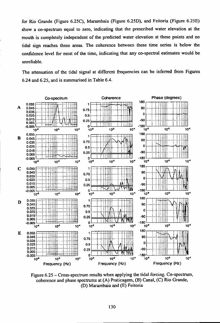
for Rio Grande (Figure 6.25C), Marambaia (Figure 6.25D), and Feitoria (Figure 6.25E)
show a co-spectrum equal to zero, indicating that the prescribed water elevation at the
mouth is completely independent of the predicted water elevation at these points and no
tidal sign reaches these areas. The coherence between these time series is below the
confidence level for most of the time, indicating that any co-spectral estimates would be
unreliable.
The attenuation of the tidal signal at different frequencies can be inferred from Figures
6.24 and 6.25, and is summarised in Table 6.4.
B
Co-spectrum 0.055 0.045 0.035 0.025 0.015 0.005
-0.005 10*
0.055 0.045 0.035 0.025 0.015 0.005
-0.005 10*
1.. J - . L i - L L L J - k . I . J . J . I J . U . L
. . . . -j-j-j-j-i^-i . . . . . i - - i --M-mi-i----- i -H-j-i-i-H-:
. . . j . . j . j . : . i . ^ j . j . i . — .
0.055 0.045 0.035 0.025 0.015 0.005
-0.005 10*
0.055 0.045 0.035 0.025 0.015 0.005
-0.005 10*
0.055 0.045 0.035 0.025 0.015 0.005 •0.005
10*
10* 10
• T - n - r r n - * - -
•1 - - r 1 - r r r r r "
• • i - i - T - i - n - r l
- T 1 - T T -o-r1
10* 10
• • ( I I I
10* 10
- r i - r r r r r -• t - 1 - t i-n-ry
i i - . i - j .
• T - - 1 - 1 - r r r r r -
10* Frequency (Hz)
10
Coherence 180
90
0
Phase (degrees)
1 - - ;;>JJ >5t* iif* ^ ^
— i . - ^ . : . i . i . ^ K . i . . . . . i . . i M - i ^ i * . :
180
90
0
.... -•i j j jiijj—A—htif?K
1 • t l l l t t l 1 • I l l t t I
-90 ..i-i-l-LLllL • t 1 <
-180 1 t i t t i i i I • i i i t t t
1 0.75 0.5
0.25
• ( - H - - : H - I - H : - : — - - j " i - i - H - x - :
• -i-ui-i" I ( I I I .
0 10*
180
90
0
-90
At-l-t-i-fi
—i-i'Trrrrrr—
10 10-
1 0.75 0.5
0.25
1 0.75 0.5
0.25
"-i"^-:-i-i-i-hi-i----4--i--j-j-i-x|
• t - -^-:-^-^)•^•^^—-J-- iH-H -Kv I : I : ::::: : : : -i--f-H-j-i-fi-j----4--i-i-i-i-x-:
0 10* 10*
Frequency (Hz) 10^ 10*
Frequency (Hz)
Figure 6.25 - Cross-spectrum results when applying the tida! forcing. Co-spectrum, coherence and phase spectrums at (A) Praticagem, (B) Canal, (C) Rio Grande,
(D) Marambaia and (E) Feitoria
130
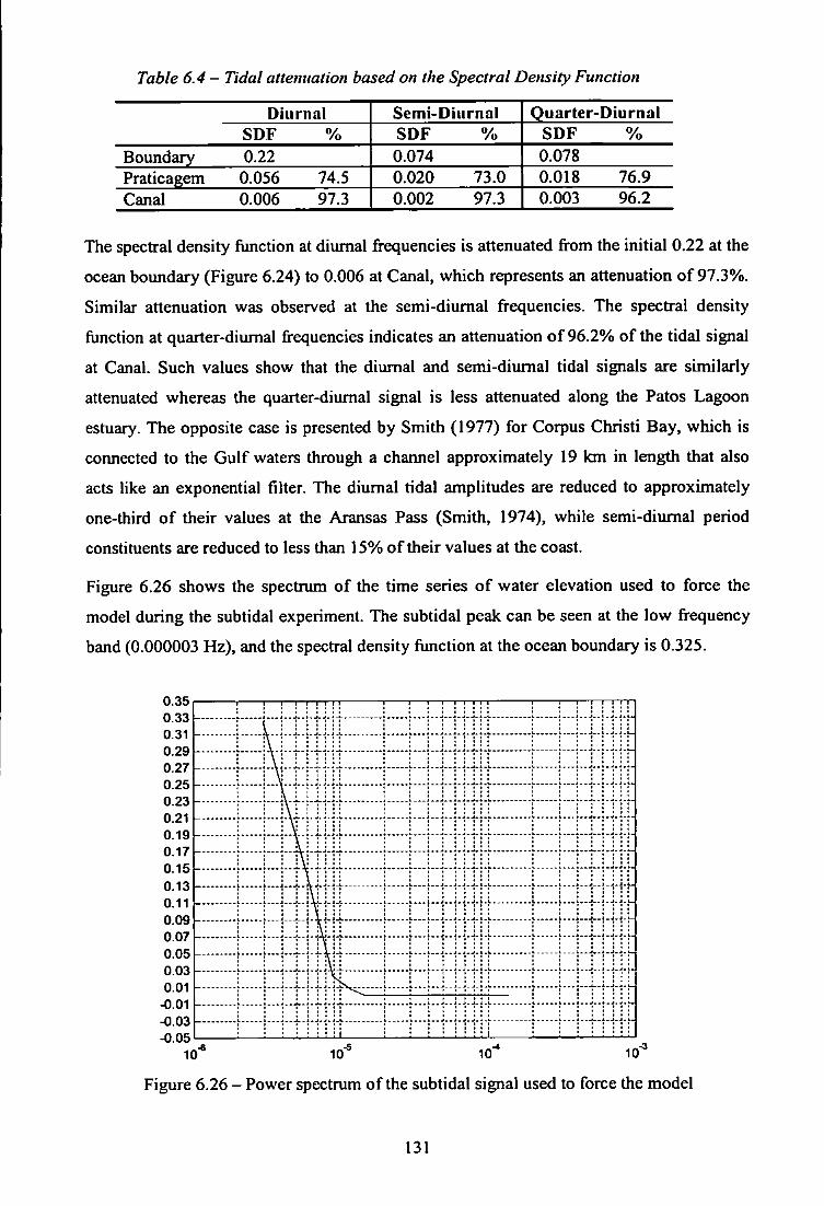
Table 6.4 - Tidal attenuation based on the Spectral Density Function
Diurnal Semi-Diurnal Quarter-Diurnal SDF % SDF % SDF %
Boundary 0.22 0.074 0.078 Praticagem 0.056 74.5 0.020 73.0 0.018 76.9 Canal 0.006 97.3 0.002 97.3 0.003 96.2
The spectral density function at diurnal frequencies is attenuated from the initial 0.22 at the
ocean boundary (Figure 6.24) to 0.006 at Canal, which represents an attenuation of 97.3%.
Similar attenuation was observed at the semi-diurnal frequencies. The spectral density
function at quarter-diumal frequencies indicates an attenuation of 96.2% of the tidal signal
at Canal. Such values show that the diurnal and semi-diumal tidal signals are similarly
attenuated whereas the quarter-diurnal signal is less attenuated along the Patos Lagoon
estuary. The opposite case is presented by Smith (1977) for Corpus Christi Bay, which is
connected to the Gulf waters through a channel approximately 19 km in length that also
acts like an exponential filter. The diurnal tidal amplitudes are reduced to approximately
one-third of their values at the Aransas Pass (Smith, 1974), while semi-diumal period
constituents are reduced to less than 15% of their values at the coast.
Figure 6.26 shows the spectrum o f the time series o f water elevation used to force the
model during the subtidal experiment. The subtidal peak can be seen at the low frequency
band (0.000003 Hz), and the spectral density function at the ocean boundary is 0.325.
T — I - I I I I
• I I •
• I > •
10 10 10 10"
Figure 6.26 - Power spectrum of the subtidal signal used to force the model
131
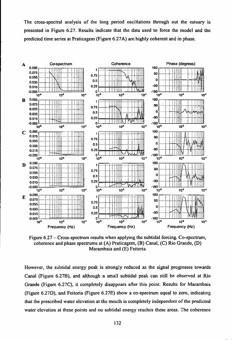
The cross-spectral analysis of the long period oscillations through out the estuary is
presented in Figure 6.27. Results indicate that the data used to force the model and the
predicted time series at Praticagem (Figure 6.27A) are highly coherent and in phase.
B
D
E
Co-spectrum Coherence Phase (degrees) 0.095
0.035 0.015
-0.005
0.075 0.055 0.035 0.015
-0.005
0.015
0.095 0.075 0.055 0.035 0.015
-0.005
0.095 0.075 0.055 0.035 0.015
-0.005
1 0.75 0.5
0.25
; I ! ! ! ! !
: :
::::::
01 1 0 * 10 10
1 0.75
0.5 0.25
10* Frequency (Hz)
10* 10* Frequency (Hz)
10^ 10* Frequency (Hz)
Figure 6.27 - Cross-spectrum results when applying the subtidal forcing. Co-spectrum, coherence and phase spectrums at (A) Praticagem, (B) Canal, (C) Rio Grande, (D)
Marambaia and (E) Feitoria
However, the subtidal energy peak is strongly reduced as the signal progresses towards
Canal (Figure 6.27B), and although a small subtidal peak can still be observed at Rio
Grande (Figure 6.27C), it completely disappears after this point. Results for Marambaia
(Figure 6.27D), and Feitoria (Figure 6.27E) show a co-spectrum equal to zero, indicating
that the prescribed water elevation at the mouth is completely independent of the predicted
water elevation at these points and no subtidal energy reaches these areas. The coherence
132
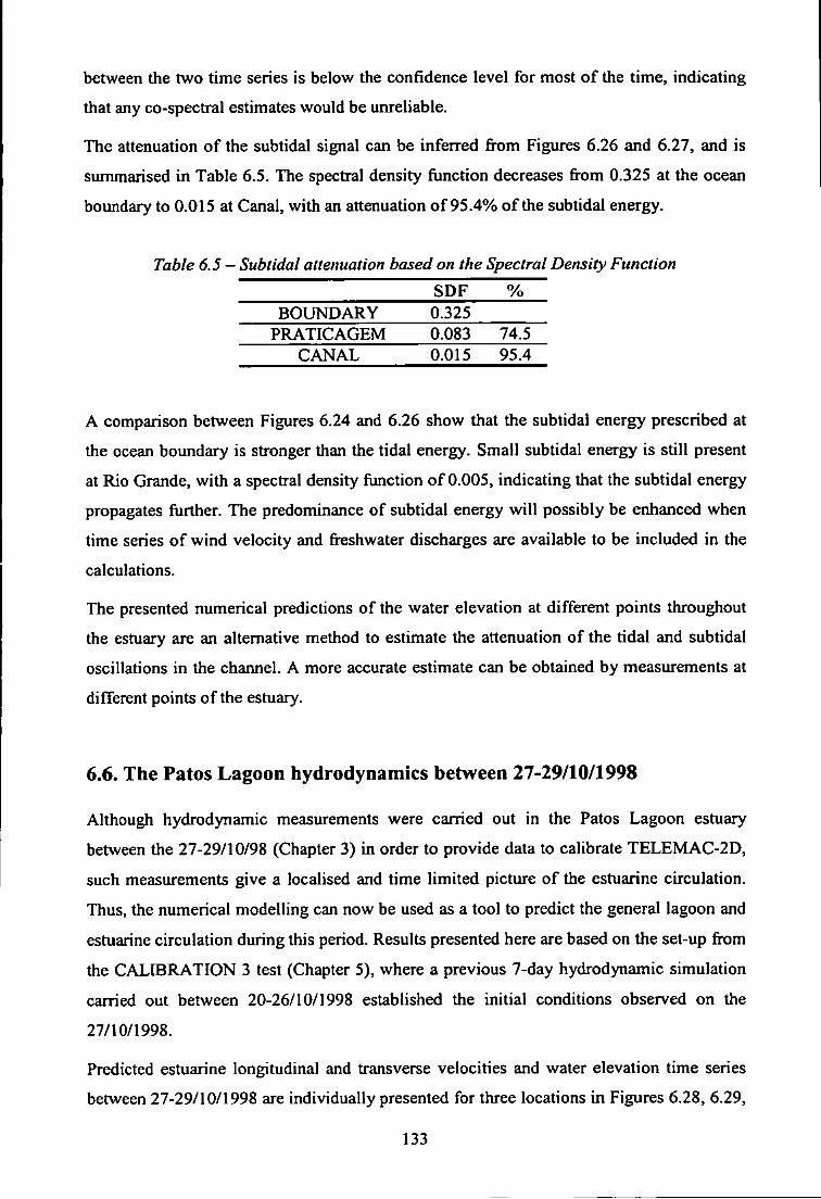
between the two time series is below the confidence level for most o f the time, indicating
that any co-spectral estimates would be unreliable.
The attenuation of the subtidal signal can be inferred from Figures 6.26 and 6.27, and is
summarised in Table 6.5. The spectral density function decreases from 0.325 at the ocean
boundary to 0.015 at Canal, with an attenuation of 95.4% of the subtidal energy.
Table 6.5- Subtidal attenuation based on the Spectral Density Function
SDF % BOUNDARY 0.325
PRATICAGEM 0.083 74.5 CANAL 0.015 95.4
A comparison between Figures 6.24 and 6.26 show that the subtidal energy prescribed at
the ocean boundary is stronger than the tidal energy. Small subtidal energy is still present
at Rio Grande, with a spectral density function of 0.005, indicating that the subtidal energy
propagates further. The predominance of subfidal energy wi l l possibly be enhanced when
time series o f wind velocity and freshwater discharges are available to be included in the
calculations.
The presented numerical predictions of the water elevation at different points throughout
the estuary are an alternative method to estimate the attenuation of the tidal and subtidal
oscillations in the channel. A more accurate estimate can be obtained by measurements at
different points of the estuary.
6.6. The Patos Lagoon hydrodynamics between 27-29/10/1998
Although hydrodynamic measurements were carried out in the Patos Lagoon estuary
between the 27-29/10/98 (Chapter 3) in order to provide data to calibrate TELEMAC-2D,
such measurements give a localised and time limited pictiu-e of the estuarine circulation.
Thus, the numerical modelling can now be used as a tool to predict the general lagoon and
estuarine circulation during this period. Results presented here are based on the set-up from
the CALIBRATION 3 test (Chapter 5), where a previous 7-day hydrodynamic simulation
carried out between 20-26/10/1998 established the initial conditions observed on the
27/10/1998.
Predicted estuarine longitudinal and transverse velocities and water elevation time series
between 27-29/10/1998 are individually presented for three locations in Figures 6.28, 6.29,
133
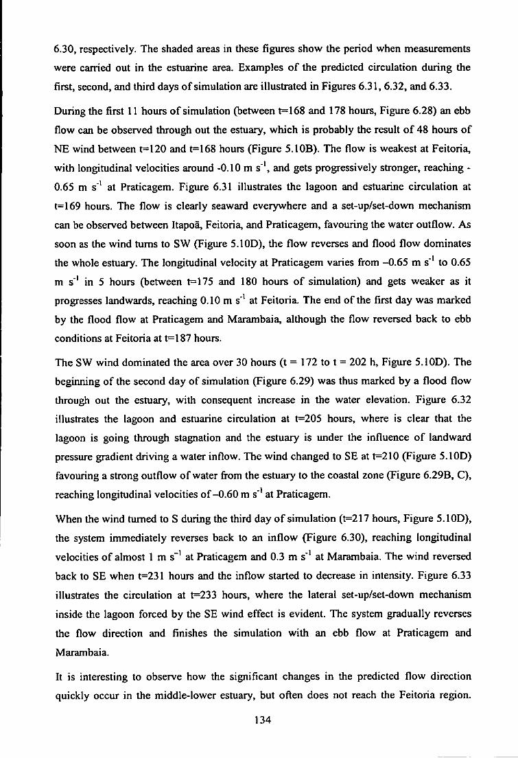
6.30, respectively. The shaded areas in these figures show the period when measurements
were carried out in the estuarine area. Examples of the predicted circulation during the
first, second, and third days of simulation are illustrated in Figures 6.31, 6.32, and 6.33.
During the first 11 hours of simulation (between t=168 and 178 hours. Figure 6.28) an ebb
flow can be observed through out the estuary, which is probably the result o f 48 hours of
NE wind between t=120 and t=168 hours (Figure 5.10B). The flow is weakest at Feitoria,
with longitudinal velocities around -0.10 m s"*, and gets progressively stronger, reaching -
0.65 m s" at Praticagem. Figure 6.31 illustrates the lagoon and estuarine circulation at
t=169 hours. The flow is clearly seaward everywhere and a set-up/set-down mechanism
can be observed between Itapoa, Feitoria, and Praticagem, favouring the water outflow. As
soon as the wind turns to SW (Figure 5.10D), the flow reverses and flood flow dominates
the whole estuary. The longitudinal velocity at Praticagem varies from -0.65 m s * to 0.65
m s ' in 5 hours (between t=175 and 180 hours of simulation) and gets weaker as it
progresses landwards, reaching 0.10 m s * at Feitoria. The end of the first day was marked
by the flood flow at Praticagem and Marambaia, although the flow reversed back to ebb
conditions at Feitoria at t=187 hours.
The SW wind dominated the area over 30 hours (t = 172 to t = 202 h, Figure 5.10D). The
beginning of the second day of simulation (Figure 6.29) was thus marked by a flood flow
through out the estuary, with consequent increase in the water elevation. Figure 6.32
illustrates the lagoon and estuarine circulation at t=205 hours, where is clear that the
lagoon is going through stagnation and the estuary is under the influence of landward
pressure gradient driving a water inflow. The wind changed to SE at t=210 (Figure 5.10D)
favouring a strong outflow of water from the estuary to the coastal zone (Figure 6.29B, C),
reaching longitudinal velocities of-0.60 m s"* at Praticagem.
When the wind turned to S during the third day o f simulation (t=217 hours. Figure 5.10D),
the system immediately reverses back to an inflow (Figure 6.30), reaching longitudinal
velocities of almost 1 m s"' at Praticagem and 0.3 m s'* at Marambaia. The wind reversed
back to SE when t=231 hours and the inflow started to decrease in intensity. Figure 6.33
illustrates the circulation at t=233 hours, where the lateral set-up/set-down mechanism
inside the lagoon forced by the SE wind effect is evident. The system gradually reverses
the flow direction and finishes the simulation with an ebb flow at Praticagem and
Marambaia.
It is interesting to observe how the significant changes in the predicted flow direction
quickly occur in the middle-lower estuary, but often does not reach the Feitoria region.
134
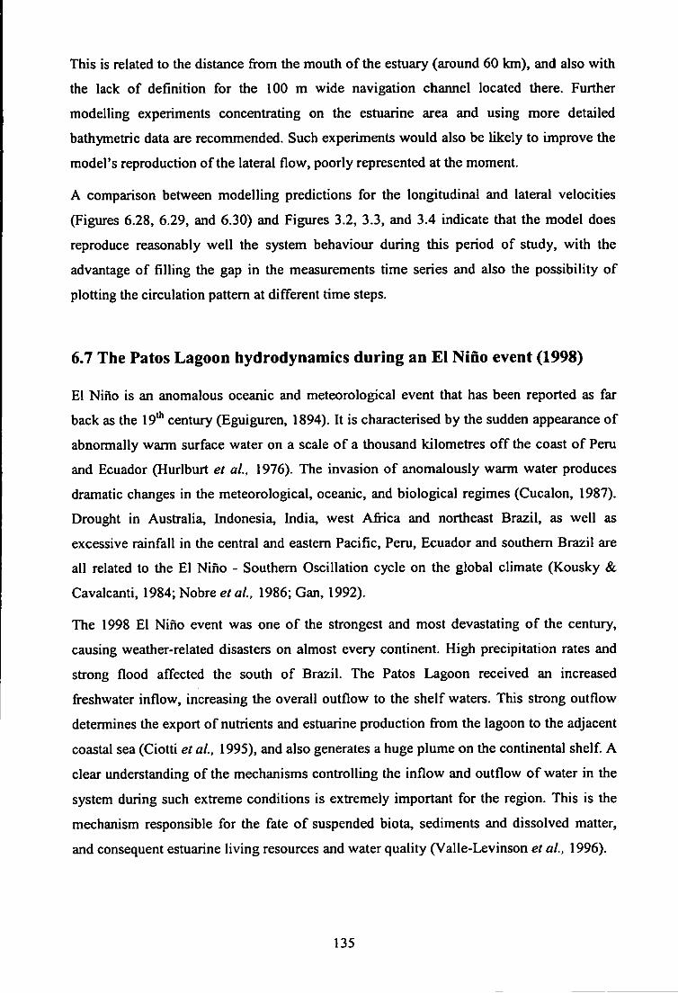
This is related to the distance from the mouth of the estuary (around 60 km), and also with
the lack of definition for the 100 m wide navigation channel located there. Further
modelling experiments concentrating on the estuarine area and using more detailed
bathymetric data are recommended. Such experiments would also be likely to improve the
model's reproduction of the lateral flow, poorly represented at the moment.
A comparison between modelling predictions for the longitudinal and lateral velocities
(Figures 6.28, 6.29, and 6.30) and Figures 3.2, 3.3, and 3.4 indicate that the model does
reproduce reasonably well the system behaviour during this period of study, with the
advantage of filling the gap in the measurements time series and also the possibility of
plotting the circulation pattern at different time steps.
6.7 The Patos Lagoon hydrodynamics during an EI Nino event (1998)
El Nino is an anomalous oceanic and meteorological event that has been reported as far
back as the 19^ century (Eguiguren, 1894). It is characterised by the sudden appearance of
abnormally warm surface water on a scale o f a thousand kilometres o f f the coast of Peru
and Ecuador (Hurlburt et al., 1976). The invasion of anomalously warm water produces
dramatic changes in the meteorological, oceanic, and biological regimes (Cucalon, 1987).
Drought in Australia, Indonesia, India, west Afi ica and northeast Brazil, as well as
excessive rainfall in the central and eastern Pacific, Peru, Ecuador and southern Brazil are
all related to the El Nino - Southern Oscillation cycle on the global climate (Kousky &
Cavalcanti, 1984; Nobre e/a/., 1986; Gan, 1992).
The 1998 El Nino event was one of the strongest and most devastating of the century,
causing weather-related disasters on almost every continent. High precipitation rates and
strong flood affected the south of Brazil. The Patos Lagoon received an increased
freshwater inflow, increasing the overall outflow to the shelf waters. This strong outflow
determines the export of nutrients and estuarine production fi-om the lagoon to the adjacent
coastal sea (Ciotti et ai, 1995), and also generates a huge plume on the continental shelf A
clear understanding of the mechanisms controlling the inflow and outflow o f water in the
system during such extreme conditions is extremely important for the region. This is the
mechanism responsible for the fate o f suspended biota, sediments and dissolved matter,
and consequent estuarine living resources and water quality (Valle-Levinson et ai., 1996).
135
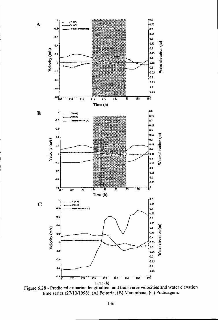
B
Vtm*)
w s o e lemon (ID)
167 170 m 176 179 182
Time (b) i&s
167 170 173 176 179 IB2
Time (h) 165
C ^
167 170
18S
Wavremaion
18S 191
UtmA) W j m e M t t n (mi
Time (h) Figure 6.28 - Predicted estuarine longitudinal and transverse velocities and water elevation
time series (27/10/1998). (A) Feitoria, (B) Marambaia, (C) Praticagem.
136
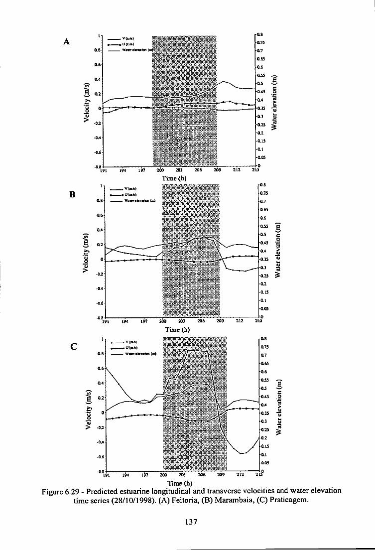
B
Waercleviton (mj
Time (h)
197 200 203 206
Time (h) 209 212 2li
Ulfnk)
191 194 197 200 203 205 209 212
Time (h) Figure 6.29 - Predicted estuarine longitudinal and transverse velocities and water elevation
time series (28/10/1998). (A) Feitoria, (B) Marambaia, (C) Praticagem.
137
B
224 227 230
Time (h)
8
•"215 218 221 224 227 230
Tinie(h)
WattratovMtan (mj
I
•"215 236 239 218 221 224 227 230 233
TuTie(h) Figure 6.30 - Predicted estuarine longitudinal and transverse velocities and water elevation
time series (29/10/1998). (A) Feitoria, (B) Marambaia, (C) Praticagem.
138
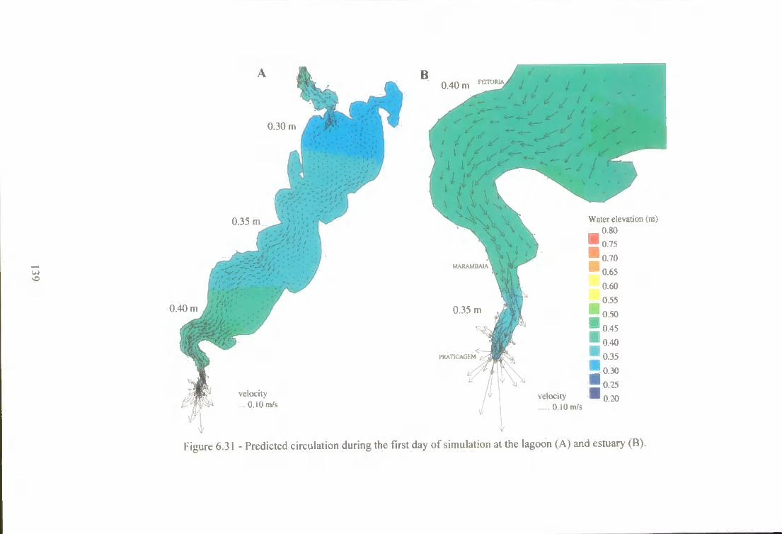
0.40 ni
0.30 m
Water elevation (m) 0.35 m
C K A I R A( .» M
velocity . 0.10 ra/!
velocity O.lOir
0.40 m
Figure 6.31 - Predicted circulation during the first day of simulation at the lagoon (A) and estuary (B).
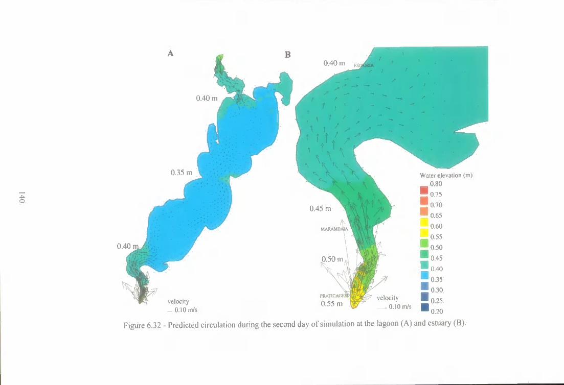
4-
0.40 m
0.40 ni
0.35 m Water elevation (m)
0.45 m
0,5
l ' k A l l L A ( . K
0.55 m velocity
. 0.10 n
0.40
velocity . 0.10 m/s
Figure 6.32 - Predicted circulation during the second day of simulation at the lagoon (A) and estuary (B).
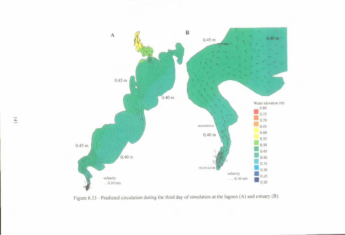
0.4. m
0.45 m
0.40 m Water clevauon (m)
0.80
l A R A M H A l A
0.40 m
0.40 ni
I ' K A I K A ( . i M
velocity 0.10 n velocity
0.10 m/i
0.45 m
Figure 6.33 - Predicted circulation during the third day of simulation at the lagoon (A) and estuary (B).
TELEMAC-2D simulations were carried out to investigate the Patos Lagoon circulation
during this period, where special attention is given to the local and non-local effects as the
most important factors controlling the exchanges between the lagoon and the continental
shelf.
Simulations were carried out based on a finite element mesh of 3697 triangles and applying
the Nikuradse law of bottom friction (^j=0.01). Imposed river flow rates of 5000, 8000 and
10000 m^ s"' were tested as the upstream boundary condition to investigate the effect o f the
freshwater discharge variation on the hydrodynamics. A time series of water elevation
measured by the Instituto Nacional de Pesquisas Hidr^ulicas (INPH) at the mouth o f the
estuary between 23/05/98 - 06/06/98 (Figure 6.34A) was prescribed at the ocean boundary,
and wind speed and direction data measured by Rio Grande Pilots (Praticagem da Barra)
for the same period of time were used to force the model (Figure 6.34B). Unfortimately, no
time series of river discharge is available.
A set-up/set-down mechanism, which combines local and non-local wind and the fluvial
discharge, is the most important factor forcing water exchanges between the lagoon and the
continental shelf. The stronger the wind and the discharge, the stronger the pressure
gradient established between the coast and Feitoria (Figuire 2.11), and the magnitude of
water advection into or out o f the lagoon (Femandes et al, in press a, c). Figure 6.35
clearly illustrates the effects of the two predominant wind situations observed in the area,
when prescribing a river inflow of 8000 m^ s * at the top end of the lagoon. When the wind
is from the SW (t=108 h), an increase in the water elevation is observed at the top of the
lagoon (Figure 6.35A), a depression is observed at the top of the estuary (Figure 6.35B),
and an increase is expected at the mouth (Figure 6.35C). The opposite behaviour is
observed at t=323 h, illustrating a NE wind event. Plots of the depth-averaged longitudinal
velocity through time indicate values around -0.3 m s"' at the top of the lagoon (Figure
6.35 A) and of the estuarine area (Figure 6.35B), and a maximum of-1.75 ms * at the mouth
of the estuary (Figure 6.35C). Moller & Castaing (1999) observed similar values for high
discharge periods. Femandes et al. (in press a, b) observed weaker velocities when
modelling the Patos Lagoon hydrodynamics under normal conditions.
Figures 6.36 and 6.37 present the spatial distribution of velocity vectors and water
elevation results after 1 and 10 days of simulation, respectively, when prescribing a river
inflow of 8000 m^ s '. The first 22 hours of simulation were dominated by wind coming
from the north quadrant, and its effect can still be observed in the lagoon after 24 hours of
142
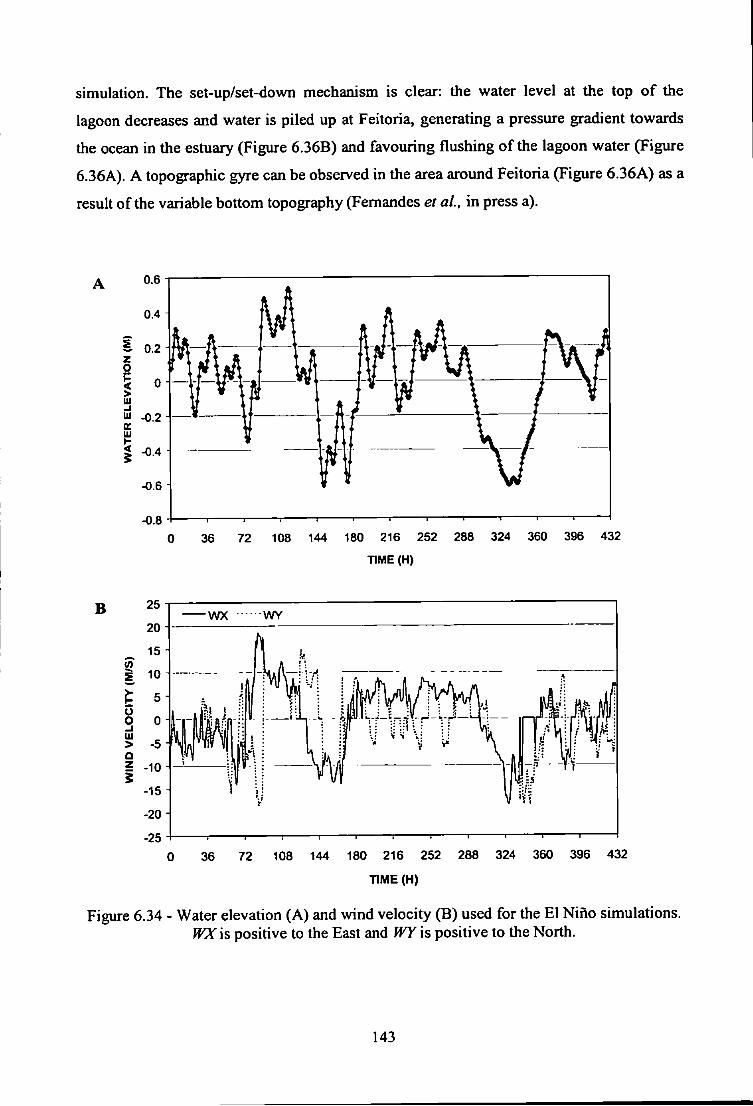
simulation. The set-up/set-down mechanism is clear: the water level at the top o f the
lagoon decreases and water is piled up at Feitoria, generating a pressure gradient towards
the ocean in the estuary (Figure 6.36B) and favouring flushing o f the lagoon water (Figure
6.36A). A topographic gyre can be observed in the area around Feitoria (Figure 6.36A) as a
result of the variable bottom topography (Femandes et al., in press a).
Ill ^.2
-0.8 0 36 72 108 144 180 216 252 288 324 360 396 432
TIME (H)
0 36 72 108 144 180 216 252 288 324 360 396 432
TIME (H)
Figure 6.34 - Water elevation (A) and wind velocity (B) used for the El Nirio simulations. WX is positive to the East and WY is positive to the North.
143
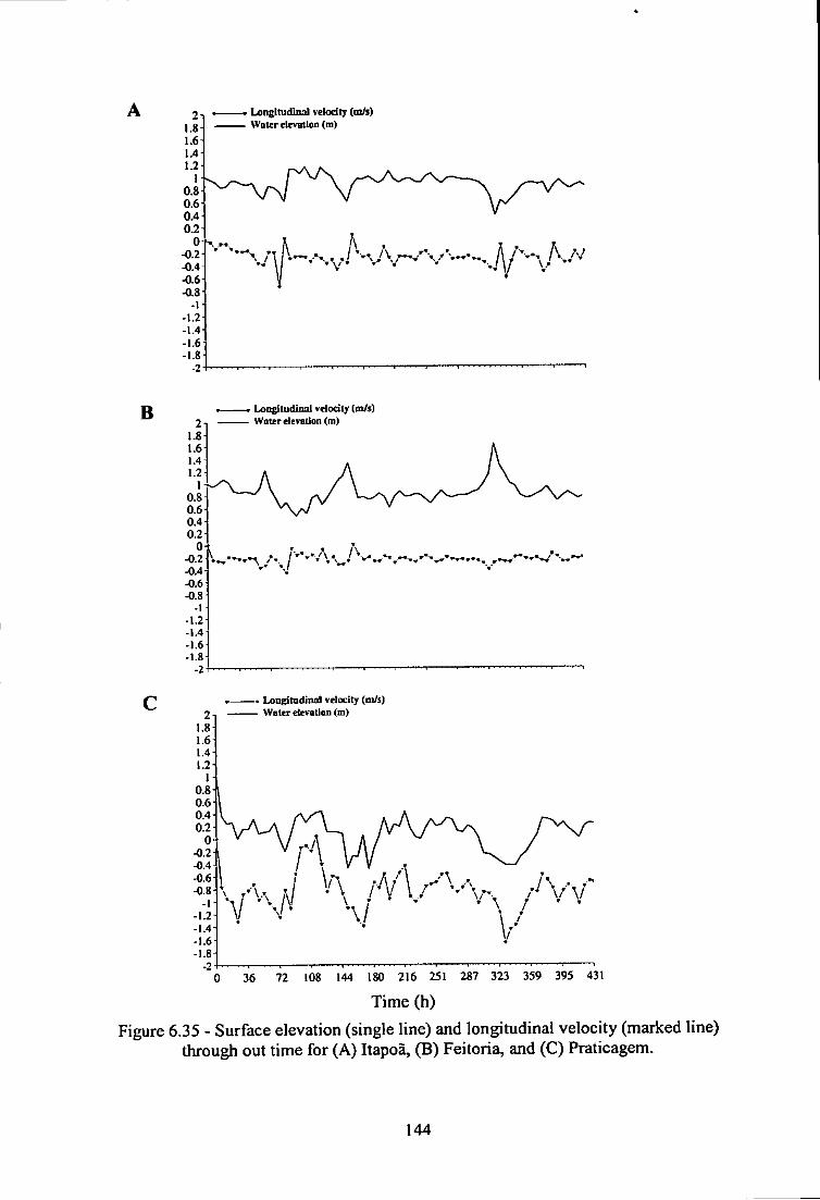
- Long[tudiiial vetodty {m/s) Water elevatloa (m)
B 2
1.8 1.6 1.4 1.2
1 0.8 0.6 0.4 0.2
0 -0.2 -0.4 -0.6 -0.8
-1 -1.2 -1.4 -1.6 -1.8
-2
Longitudiiml velocity (m^) Water elevation <ra)
2-1.8 1.6 1.4 1.2
1 0.8 0.6 0.4 0.2
0 -0.2 -0.4 -0.6 -0.8
-1.2 -1.4 -1.6 -1.8
-2
Lon^tudJnal velocity (m/s) Water ele\-atJon (m>
v
36 72 108 144 180 216 251 287 323 359 395 431
Time (h)
Figure 6.35 - Surface elevation (single line) and longitudinal velocity (marked line) through out time for (A) Itapoa, (B) Feitoria, and (C) Praticagem.
144
After 10 days of simulation (Figure 6.37), the NW wind generates a lateral set-up/set-down
mechanism inside the lagoon (Figure 6.37B), where an increase in the water elevation at
the right margin and a decrease at the left 3XQ observed when looking up the estuary. The
estuarine area maintains a pressure gradient towards the ocean. The velocity vectors along
the lagoon and estuary (Figure 6.37A) indicate that velocities are seawards everywhere and
intensified in the estuarine and nodal area (Arambare, Figure 2.3). Strong velocities can be
observed at the top of the lagoon due to the prescribed fi-eshwater discharge, and the gyres
are not observed.
The exchange of water between estuaries and the inner continental shelf occurs over a wide
range of time scales and in response to a variety of astronomical, thermodynamic and
meteorological forces (Smith, 1978). Valle-Levinson et aL, (1996) comment about the
importance of clearly understanding the inflow and outflow of water in an estuary, because
this is the mechanism responsible for the fate of suspended biota, sediments and dissolved
matter, and consequently estuarine living resources and water quality.
The lagoon residence time can be defined as the time required to replace the existing
volume of fi*eshwater at a rate equal to the river discharge (Dyer, 1997). Moller (1996)
calculated a residence time of one year and a half for a mean annual fi'eshwater discharge
of 1000 m^ s"', indicating a quite long renewal process within the lagoon. During the El
Nino hydrodynamic simulations, the Patos Lagoon had an initial volume of 58,547.27 x
10* m , resulting in a residence time of 135, 85, and 68 days when considering a river
inflow of 5000. 8000 and 10000 m^ s"', respectively.
Figure 6.38 shows the variation in the lagoon volume through fime against the water
elevation (Figure 6.38A) and wind velocity (Figure 6.38B) data used to force the model
during the El Nino simulations, when prescribing a river inflow of 5000 m s'\ The
beginning of the simulation is dominated by NE wind, favouring flushing out the lagoon
waters and decreasing the volume. The first sudden variation of volume in the lagoon
happens between 72 and 84 hours. In the beginning, the combination of the north quadrant
wind and the water elevation variation fi-om -0.14 (t=72 h) to -0.28 m (t=78 h) at the mouth
generates a pressure gradient towards the ocean, favouring flushing water out of the
lagoon. Although the wind remains fi-om the north quadrant, the water elevation between
78 and 84 hours decreases to -0.06 m due to the non-local effect, reversing the pressure
gradient landwards and increasing the volume of the lagoon by 430.8 x 10* m .
145
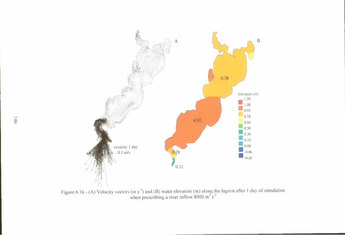
- I -0^
velocity
Elevation (m) ,.20 ..06
• 0 . 9 2 0.78
U M
• 0 . 5 0 •0.36 J 0.22
'-0.06 '-0.20
0.22
Figure 6.36 - (A) Velocity vectors (m s ') and (B) water elevation (m) along the lagoon after I day of simulation when prescribing a river inflow 8000 m s
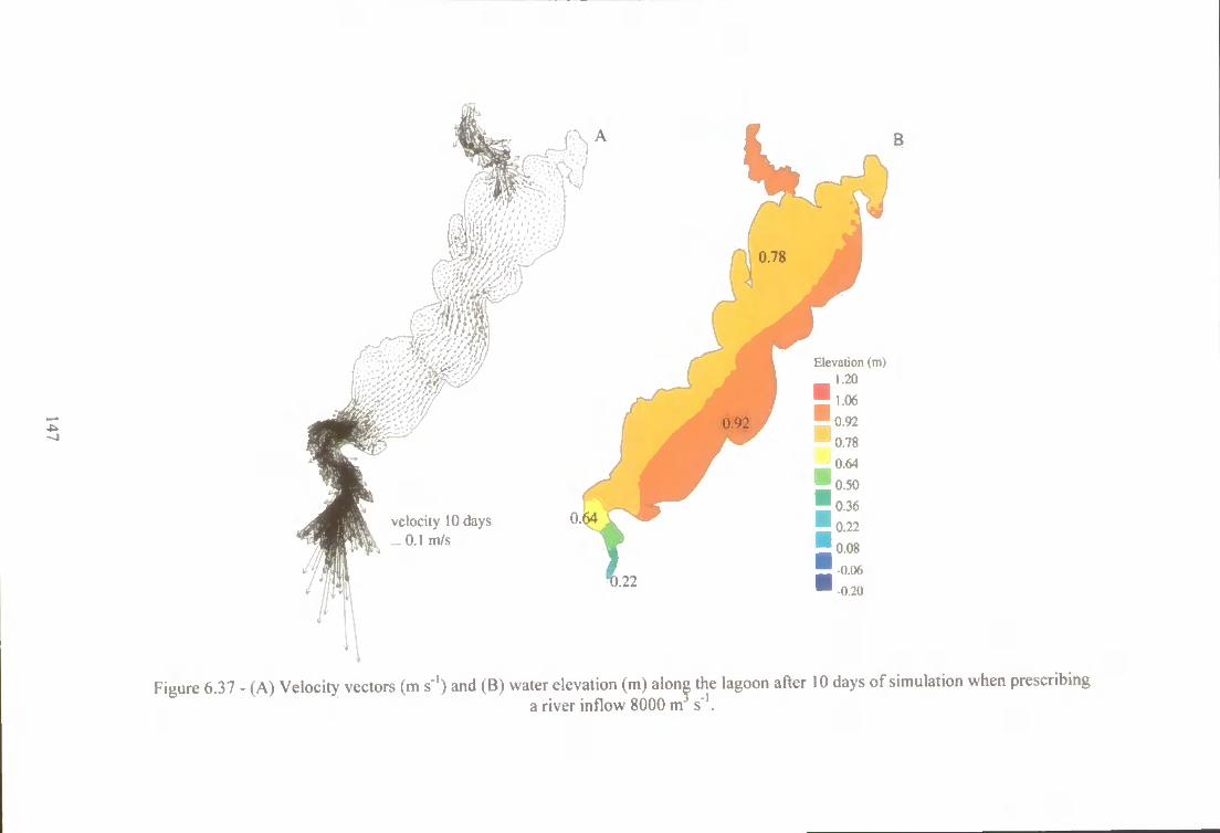
velocity 10 days O.l m/s
blevat jon ( m )
Figure 6.37 - (A) Velocity vectors (m s') and (B) water elevation (m) alone the lagoon after 10 days of simulation when prescribing a river inflow 8000m s"V
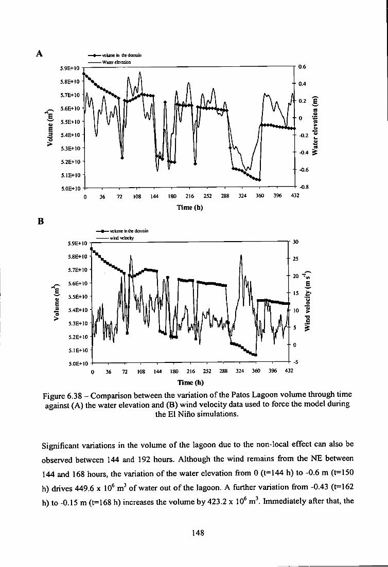
• wlime 11 the donmi •Water elcvatfan
5.9E^-10
5.8E4-10
5.7E4-10
^ 5.6E4-10
5.5E+10 i
= 5.4E4-10 1
5.3E^-10
5.2E+10
5.1E4-10
5.0E+10
B
36 72 108 144 180 216 252 288 324 360 396 432
Time (h)
• wkmK in (he doimii
•vivd vcbcty 5.9E+10
5.8E^-10
5.7E+10
5.6E+10
5.5E+10
5.4E+10
5.3E+10
5.2E+10
5.IE+10
5.0E+10 36 72 108 144 180 216 252 288 324 360 396 432
Hme (h)
Figure 6.38 - Comparison between the variation of the Patos Lagoon volume through time against (A) the water elevation and (B) wind velocity data used to force the model during
the E l Nino simulations.
Significant variations in the volume of the lagoon due to the non-local effect can also be
observed between 144 and 192 hours. Although the wind remains fi-om the NE between
144 and 168 hours, the variation of the water elevation from 0 (t=I44 h) to -0.6 m (t=150
h) drives 449.6 x 10** m of water out of the lagoon. A further variation from -0.43 (t=162
h) to -0.15 m (t=168 h) increases the volume by 423.2 x 10 m\ Immediately after that, the
148
wind slows down and a non-local variation in the water elevation promotes similar volume
variations.
A situation where the local wind forcing dominates the circulation can be observed
between 306 and 360 hours. Previously, a decrease in the water elevation from 0.08 (t=294
h) to -0.33 m (t=306 h) favours the flushing of the lagoon, but between 306 and 360 hours
the dynamics is controlled by the strong N E predominant wind and more water is pumped
out, although further variations on the water elevation were still observed. When the wind
slows down (t=360 h), the non-local effect becomes dominant again, and a variation of
water elevation from -015 (t=360 h) to -0.02 m (t=366 h) reverses the pressure gradient
landwards and increases the volume by 410.4 x 10* m .One important issue in this study is
characterising the volume of water transported through the entrance of the estuary during
the study period. A general view of the Patos Lagoon hydrodynamics during this high
discharge period shows volumes of water in the order of 420 x 10* m"', which represents
approximately 7% of the lagoon initial volume, being stored in or flushed out of the lagoon
in several events, in time intervals as small as 6 hours. When correlating the local and non
local forcing with the variation of volume in the lagoon through time, a correlation of 0.74
was observed for the water elevation and 0.39 for the longitudinal wind, indicating that the
non-local forcing dominates the exchanges between the estuary and the adjacent coastal
sea. A comparison between the initial and final volume of the lagoon indicates that outflow
dominates inflow, with a decrease of 4,215.62 x 10* m^ in the total volume during the 18
days of simulation, confirming the long-term seaward residual flow commented by Moller
(1996).
Several authors discuss the processes controlling the inflow/outflow of water in estuaries.
Weisberg (1976) observed that the wind effect in the water exchange process of the
Providence River of Narragansett Bay can be of equal or greater importance to the tidal or
the gravitational circulation. Smith (1977) conmients that Ekman transport controls the
meteorologically forced exchanges between the Gulf of Mexico and Corpus Christi Bay,
where the system looses as much as 10 % of its total volume during one specific frontal
passage. Valle-Levinson (1995) explores the baroclinic and barotropic exchanges in the
lower Chesapeake Bay, whereas Valle-Levinson et al, (1996) comment that the lower
Chesapeake Bay responds barotropically to local winds and coastal Ekman flux (Wang &
Elliot 1978; Wang 1979), producing inflows/outflows larger than those produced by the
estuarine circulation and river discharge.
149
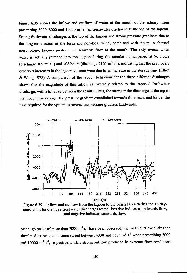
Figure 6.39 shows the inflow and outflow of water at the mouth of the estuary when
prescribing 5000, 8000 and 10000 m s"* of freshwater discharge at the top of the lagoon.
Strong freshwater discharges at the top of the lagoon and strong pressure gradients due to
the long-term action of the local and non-local wind, combined with the main channel
morphology, favours predominant seawards flow at the mouth. The only events when
water is actually pumped into the lagoon during the simulation happened at 96 hours
(discharge 369 m^ s ') and 108 hours (discharge 2161 m^ s'*), indicating that the previously
observed increases in the lagoon volume were due to an increase in the storage time (Elliot
& Wang 1978). A comparison of the lagoon behaviour for the three different discharges
shows that the magnitude of this inflow is inversely related to the imposed freshwater
discharge, with a time lag between the results. Thus, the stronger the discharge at the top of
the lagoon, the stronger the pressure gradient established towards the ocean, and longer the
time required for the system to reverse the pressure gradient landwards.
SOOOCUITBCS 8000 cunrcs 10000 cumecs
4000
2000 -
mou
l
0 -
n -2000 -
flow
3 o
-4000 -%
Infl
oi
-6000 -
8000 180 216 252 288 324 396 432
Time (h) Figure 6.39 - Inflow and outflow from the lagoon to the coastal area during the 18 day-simulation for the three freshwater discharges tested. Positive indicates landwards flow,
and negative indicates seawards flow.
Although peaks of more than 7000 m^ s * have been observed, the mean outflow during the
simulated extreme conditions varied between 4330 and 5585 m^ s * when prescribing 5000
and 10000 m^ s'\ respectively. This strong outflow produced in extreme flow conditions
150
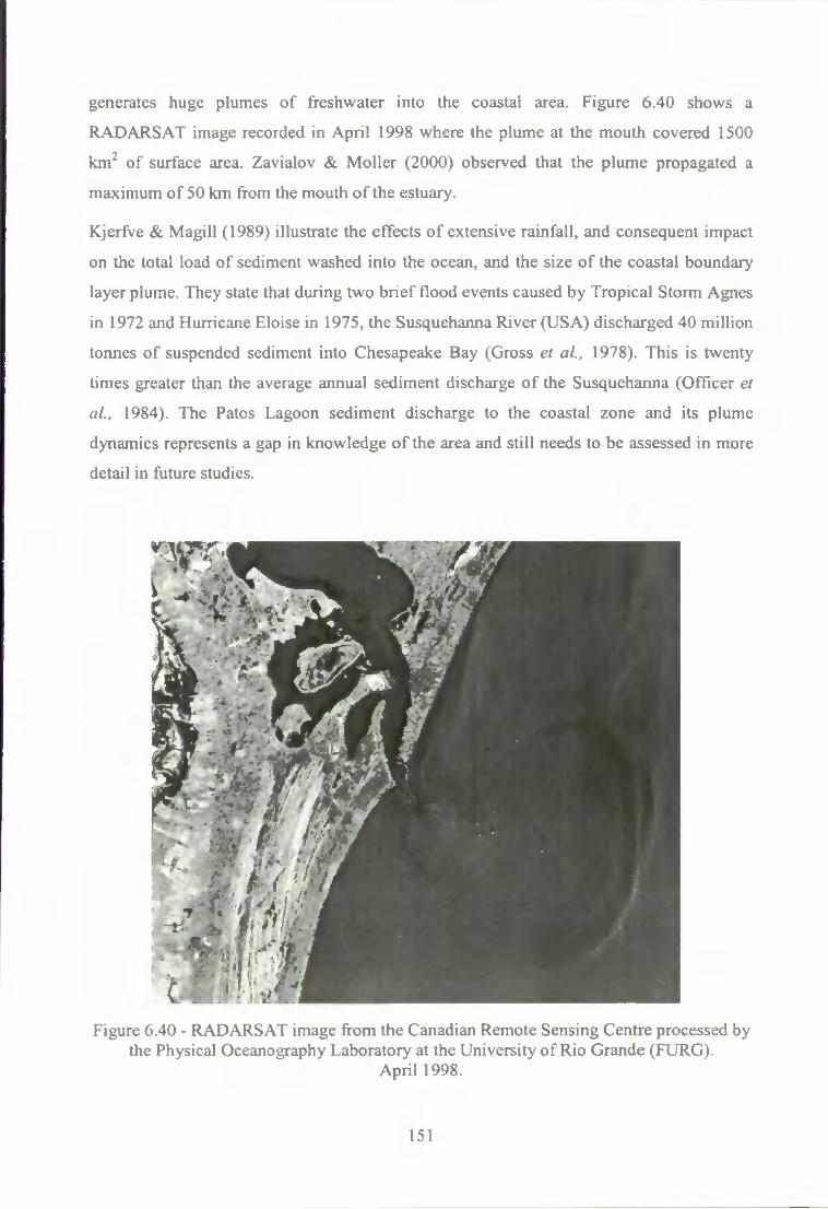
generates huge plumes of freshwater into the coastal area. Figure 6.40 shows a
RADARS AT image recorded in April 1998 where the plume at the mouth covered 1500
km^ of surface area. Zavialov & Moller (2000) observed that the plume propagated a
maximum of 50 km from the mouth of the estuary.
Kjerfve & Magill (1989) illustrate the effects o f extensive rainfall, and consequent impact
on the total load of sediment washed into the ocean, and the size of the coastal boundary
layer plume. They state that during two brief flood events caused by Tropical Storm Agnes
in 1972 and Hurricane Eloise in 1975, the Susquehanna River (USA) discharged 40 million
tonnes of suspended sediment into Chesapeake Bay (Gross et al., 1978). This is twenty
times greater than the average annual sediment discharge of the Susquehanna (Officer et
al., 1984). The Patos Lagoon sediment discharge to the coastal zone and its plume
dynamics represents a gap in knowledge of the area and still needs to be assessed in more
detail in future studies.
Figure 6.40 - RADARSAT image from the Canadian Remote Sensing Centre processed by the Physical Oceanography Laboratory at the University of Rio Grande (FURG).
April 1998.
151
Chapter 7
The Fatos Lagoon Three-dimensional Circulation
7.1. Introduction
This chapter presents the TELEMAC-3D application to the Patos Lagoon in order to better
understand its three-dimensional circulation. Initially, results from two vertical cross-
sections in the estuary are presented to illustrate the effect of barotropic forces on the
longitudinal flow and the possible mechanisms involved in the estuarine transverse
circulation diuing the two predominant wind situations. Secondly, the model takes into
account the baroclinic forces and a salinity penetration event is explained based on the
observed barotropic forces. Finally, the three-dimensional numerical modelling of salinity
distribution in the estuary is used to qualitatively estimate the intensity of mixing occurring
at difTerent times and at different positions in the estuary based on the predicted
Richardson number.
7.2. Longitudinal and Transverse Flow in the Estuary
\n order to simulate the flow features in the vertical during constant NE and SW wind
events, three-dimensional modelling experiments were carried out applying T E L E M A C -
3D. The model was forced by a dynamic boundary condition at the ocean boundary, using
water elevation data from Praticagem between 11-13/01/1992 (Figure 5.1), and by
prescribing a water inflow of 2000 m"' s'* at the top end of the lagoon. Simulations were
carried out based on a finite element mesh of 1892 triangles. Results were plotted for
vertical cross sections A and B in the estuarine area (Figure 7.1).
Figure 7.2 shows a vertical section at Feitoria (Figure 7.1, section A) when prescribing a
constant 7 m s * wind from the NE, where contours represent the along-estuary flow and
vectors represent the cross-estuary flow. Plots on the top of each cross section show the
corresponding free surface elevation. Results show seaward flow through the whole water
column (contours) after 5 h of simulation (Figure 7.2A), being stronger at the surface (0.08
m s"' in the shallow areas and 0.03 m s"* in the deep areas, and very weak at the bottom
(almost zero). During the rest of the simulation the longitudinal flow remained seawards,
152
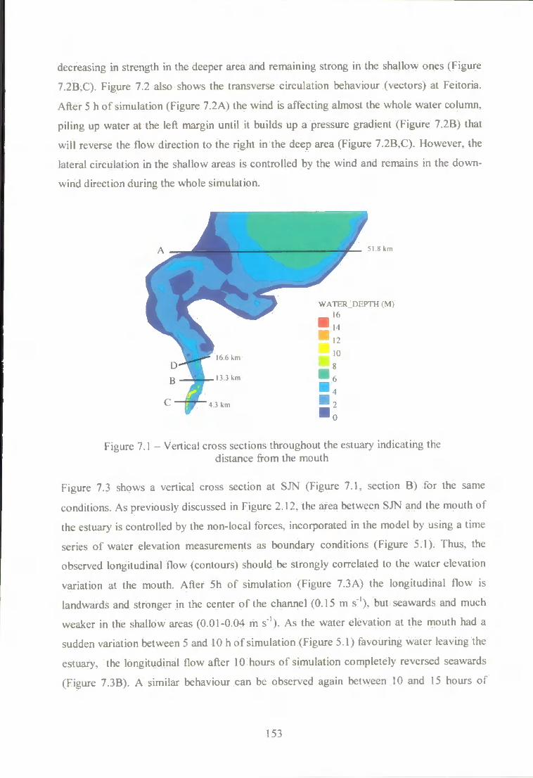
decreasing in strength in the deeper area and remaining strong in the shallow ones (Figure
7.2B.C). Figure 7.2 also shows the transverse circulation behaviour (vectors) at Feitoria.
After 5 h of simulation (Figure 7.2A) the wind is affecting almost the whole water column,
piling up water at the left margin until it builds up a pressure gradient (Figure 7.2B) that
wil l reverse the flow direction to the right in the deep area (Figure 7.2B,C). However, the
lateral circulation in the shallow areas is controlled by the wind and remains in the down
wind direction during the whole simulation.
5 1 8 k m
W A r r . R n i ' K i H ( M )
166 km
3 3 km
4 3 km
Figure 7.1 - Vertical cross sections throughout the estuary indicating the distance from the moulh
Figure 7.3 shows a vertical cross section at SJN (Figure 7.1, section B) for the same
conditions. As previously discussed in Figure 2.12, the area between SJN and the mouth of
the estuary is controlled by the non-local forces, incorporated in the model by using a time
series of water elevation measurements as boundary conditions (Figure 5.1). Thus, the
observed longitudinal flow (contours) should be strongly correlated to the water elevation
variation at the mouth. After 5h of simulation (Figure 7.3A) the longitudinal flow is
landwards and stronger in the center of the channel (0.15 m s"'), but seawards and much
weaker in the shallow areas (0.01-0.04 m s"'). As the water elevation at the mouth had a
sudden variation between 5 and 10 h of simulation (Figure 5.1) favouring water leaving the
estuary, the longitudinal flow after 10 hours of simulation completely reversed seawards
(Figure 7.3B). A similar behaviour can be observed again between 10 and 15 hours of
153
simulation, resulting in another change in the longitudinal flow direction (Figure 7.3C),
and also in the last hours of simulation (Figure 7.3D).
Figure 7,3 also shows the transverse circulation behaviour (vectors) at SJN. This
circulation seems to be related to the channel curvature and to variations in the longitudinal
flow direction. For example, the landwards flow observed in the first 5 hours of simulation
(Figure 7.3A) interacts with the curved channel and is driven to the left margin, generating
an increase in the free surface elevation. The reverse mechanism is observed everytime the
longitudinal flow changes its direction (Figure 7.3B, C. D).
Figure 7.4 shows the vertical cross section at Feitoria (Figure 7.1, section A) when
prescribing a constant 7 m s"' SW wind, where contours represent the along-estuary flow
and vectors represent the cross-estuary flow and plots on the top of each cross section
show the corresponding free surface elevation. Results show landward flow throughout the
whole water column (contours) after 5 h of simulation (Figure 7.4A), being stronger at the
surface (0.14 m s"' at the shallow areas and 0.03 m s"* in the deep areas), and very weak at
the bottom (ahnost zero). Diuing the rest of the simulation the longitudinal flow remained
landwards, always stronger in the shallow areas (Figure 7.4B,C). Figure 7.4 also shows the
transverse circulation behaviour (vectors) at Feitoria. The initial SW wind effect (Figure
7.4A) drives the secondary flow to the right in the whole water column and the
longitudinal flow accumulates water at the left margin, generating a pressure gradient
towards the right. Figure 7.4B shows that after 10 hours this pressure gradient remains, but
gets weaker, and the flow direction starts to reverse at the bottom. A comparison between
Figures 7.2 and 7.4 show that when the wind comes from NE the secondary flow has its
down-wind direction completely reversed before 10 hours of simulation (Figure 7.2B),
while for SW winds reversion of the down-wind secondary flow starts to happen after 10
hours of simulation (Figure 7.4B), being potentially related to the seaward flow observed
at the bottom. A strong pressure gradient starts to build after 10 hours of simulation (Figure
7.4B) and increases towards the end of the simulation (Figure 7.4C). However, the
secondary circulation in the shallow areas is still controlled by the wind and remains in the
down wind direction during the whole simulation.
Figure 7.5 shows the vertical cross section at SJN (Figure 7.1, section B) when prescribing
a constant 7 m s * SW wind. As commented before for Figure 7.3, the observed
longitudinal flow (contours) is expected to be strongly correlated to the water elevation
variation at the mouth. However, when prescribing the wind from the SW in the model, the
154
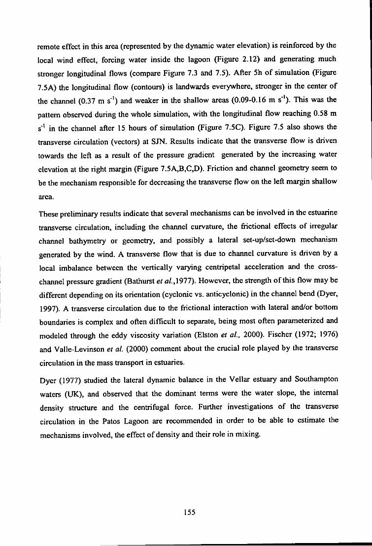
remote effect in this area (represented by the dynamic water elevation) is reinforced by the
local wind effect, forcing water inside the lagoon (Figure 2.12) and generating much
stronger longitudinal flows (compare Figure 7.3 and 7.5). After 5h of simulation (Figure
7.5A) the longitudinal flow (contours) is landwards everywhere, stronger in the center of
the channel (0.37 m s"*) and weaker in the shallow areas (0.09-0.16 m s"*). This was the
pattern observed during the whole simulation, with the longitudinal flow reaching 0.58 m
s'* in the channel after 15 hours of simulation (Figure 7.5C). Figure 7.5 also shows the
transverse circulation (vectors) at SJN. Results indicate that the transverse flow is driven
towards the left as a result of the pressure gradient generated by the increasing water
elevation at the right margin (Figure 7.5A,B,C,D). Friction and channel geometry seem to
be the mechanism responsible for decreasing the transverse flow on the left margin shallow
area.
These preliminary results indicate that several mechanisms can be involved in the estuarine
transverse circulation, including the channel curvature, the frictional effects of irregular
channel bathymetry or geometry, and possibly a lateral set-up/set-down mechanism
generated by the wind. A transverse flow that is due to channel curvature is driven by a
local imbalance between the vertically varying centripetal acceleration and the cross-
channel pressure gradient (Bathurst et a/., 1977). However, the strength of this flow may be
different depending on its orientation (cyclonic vs. anticyclonic) in the channel bend (Dyer,
1997). A transverse circulation due to the fnctional interaction with lateral and/or bottom
boundaries is complex and often difficult to separate, being most often parameterized and
modeled through the eddy viscosity variation (Elston et al., 2000). Fischer (1972; 1976)
and Valle-Levinson et al. (2000) comment about the crucial role played by the transverse
circulation in the mass transport in estuaries.
Dyer (1977) studied the lateral dynamic balance in the Vellar estuary and Southampton
waters (UK), and observed that the dominant terms were the water slope, the internal
density structure and the centrifugal force. Further investigations of the transverse
circulation in the Patos Lagoon are recommended in order to be able to estimate the
mechanisms involved, the effect of density and their role in mixing.
155
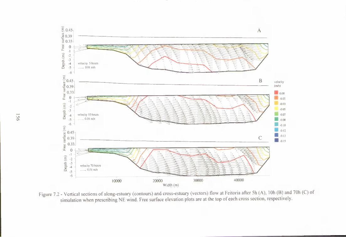
S 0.45
velocity 5 hours 0.01 m/s
(m/s)
-001
vclociiy 10 houn
. 0.01 mJi
vckxity
10000 2()(XK) Mm) 40000 Width (m)
Figure 7.2 - Vertical sections of along-estuary (contours) and cross-estuary (vectors) flow at Feitoria after 5h (A), lOh (B) and 70h (C) of simulation when prescribing NE wind. Free surface elevation plots are at the top of each cross section, respectively.
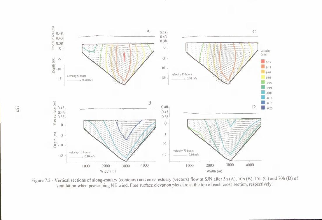
- J
E « 0.48 I 0.43 I 0.38 I 0
I |--io
-15
[ ' ' / • • Krf ' / ' •
V ' - 1 / ^ ^ . * —^ r
velocity 5 hours
> 0.10 m/s
S ^0.48 I 0.43 S 0.38
0 ]
I -5
10 \
15 velocity 10 hours
> 0.10 m/i
ICXX) 2000 Width (m)
MXK)
0.48 0.43 0.38
0
-5
-10
-15 velocity 15 hours
». 0.10 m/s
velocity
velocity 70 hours
» . 0 . 1 0 n i / 8
KKH) 2000 3000
Width (m)
4 ( X X )
Figure 7.3 - Vertical sections of along-estuary (contours) and cross-estuary (vectors) flow at SJN after 5h (A), lOh (B), 15h (C) and 70h (D) of simulation when prescribing NE wind. Free surface elevation plots are at the top of each cross section, respectively.
0 0
velocio
veliKiiv htwin
velocity 70 hours 0.01 m/i
I t K H H * 2(XXX) 30000 Widlh (m)
S(MKX)
Figure 7.4 - Vertical sections of along-estuary (contours) and cross-estuary (vectors) flow at Feitoria after 5h (A), lOh (B) and 70h (C) of simulation when prescribing SW wind. Free surface elevation plots are at the top of each cross section, respectively.
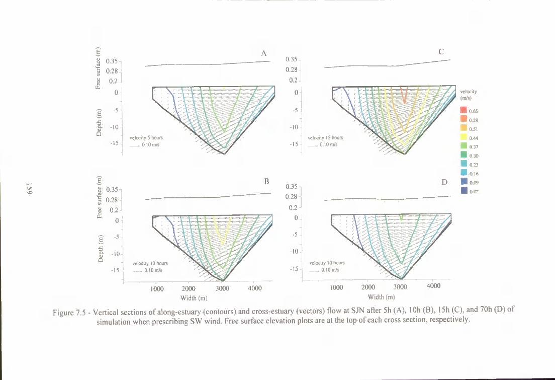
so
£
-5
0.35 0.28 0.2
0
-5
-10
-15
e \ 0.35
% 0.28
0.2
0
6 -5
•10
•15
velocity 5 hours . 0.10 m/s
velocity
velocity IS houn 0.10 m/s
velocity 70 houn
0.10 m/s velocity 10 hours
. 0.10 m/s
I ( X X ) 2000 Width (m)
3000 t(MH) 1000 2000 3000 Width (m)
4 ( K K )
Figure 7.5 - Vertical sections of along-estuary (contours) and cross-estuary (vectors) flow at SJN after 5h (A), lOh (B), 15h (C), and 70h (D) of simulation when prescribing SW wind. Free surface elevation plots are at the top of each cross section, respectively.
The knowledge of this role can help to better predict important parameters such as the
length of the salt intrusion and to determine the dispersion of larvae, sediment and
pollutants in the estuarine environment (Elston et al., 2000).
Csanady (1973) and Kjerfve & Magill (1989), among many others, have shown that the
wind stress applied at the surface of a basin of variable depth sets up a circulation pattern
characterised by relatively strong barotropic coastal currents in the direction of the wind,
with return flow occuring over the deeper regions. However, this seems not to be the case
for the Patos Lagoon when simulating simple situations of temporally and spatially
constant wind. The authors believe that when simulating the lagoon three-dimensional
behaviour with a more comprehensive data set (including density effects and time series of
wind speed and direction to force the model), a more detailed picture of the circulation can
be observed. Unfortunately a more comprehensive data set is not available for the period
between 11-13/01/1992.
Results also indicate that three-dimensional simulations are essential to study the
transverse circulation in the lagoon. Dyer (1977) comments how difficult it is to study the
components of the secondary circulation using measurements, and Fischer (1972; 1976)
comments about the limitation of a two-dimensional numerical approach for this purpose.
It is also important to notice that cross sections presented in Figures. 7.2 - 7.5 are not
normal to the mean flow direction. Further analysis of the cross section orientation is
necessary before other studies of the transverse circulation are carried out in the area.
7.3. Modelling salinity distribution in the estuary
Coastal lagoons are usually considered as a well-mixed type of estuaries. The wind action
over shallow water bodies combined with low river discharge are the main factors
responsible for that.
Stratification and destratification cycles in estuaries have been reported to be due: to
relative strength of river and wind action (Schroeder et ai, 1990), to strong v^nd events
(Goodrich et ai, 1987) and to river flow action (Smith, 1985). In the case of the Patos
Lagoon, it depends mainly on the relative strength of the barotropic circulation induced by
the wind field and river flow (MoUer & Castaing, 1999), but the morphology of the Patos
Lagoon may also play an important role. The funnelling in the lagoon section tends to
160
enhance the effect of river flow, and the access channel (14 m deep) may contribute to the
flow separation in a two-layered vertical structure. Moller & Castaing (1999) comment that
well-mixed conditions can be observed in the inlet even during periods of high river flow
(> 4000 m"* s"') during the passage of a strong cold front that forces large amounts of
coastal water to enter the lagoon.
Three-dimensional simulations were carried out for the Patos Lagoon in order to
complement the hydrodynamic information obtained for the period when measurements
were carried out in the estuary (27-29/10/1998). Results presented here are based on the
same set-up used in Section 6.6. However, salinity is now taken into account as a tracer
prescribed at the ocean boundary, having a constant value of 28 psu throughout the water
column. The time series of water elevation and wind velocity used to force the model are
presented in Figure 7.6 to better illustrate the barotropic effects during this period.
Plots throughout time from a vertical cross-section located 4.5 km from the mouth of the
estuary (section C, Figure 7.1) show the main flow direction (Figure 7.7) and salinity
distribution (Figure 7.8) during the first 34 hours of simulation. After 10 hours of
simulation, the combination of SW wind and high water elevation at the mouth (Figure
7.6) favoured a landward pressure gradient, with flood flow dominating the channel area
and starting to force salinity penetration in the channel (Figures 7,7A and 7.8A). Some ebb
flow can be observed in the surface and shallow areas as a result of a previous NE wind
period. As the prescribed SW wind and water elevation at the mouth start to decrease
(Figure 7.6), the ebb flow in the surface is enhanced after 16 hours of simulation (Figure
7.7B). A flood flow remains in the channel, enhancing salinity penetration and creating a
vertically stratified estuary with salinity varying from 28 to 12 (Figure 7.8B). The shallow
area is characterised by lateral stratification.
Winds from the SW were dominant (Figure 7.6B) and the flooding and stratified
conditions dominated the whole water column after 22 hours of simulation (Figure 7.7C
and 7,8C). The inflow of water into the channel is clear but as the SW wind velocity
decreases, the inflow becomes more homogeneous in the channel and stronger in the
shallow areas (Figure 7.7D,E). Vertical stratification in the channel also decreases (Figure
7.8D), reaching a well-mixed condition after 34 hours (Figure 7.8E), while salinity keeps
increasing in the shallow areas and maintaining the lateral stratification condition due to
stronger inflow over the area.
161
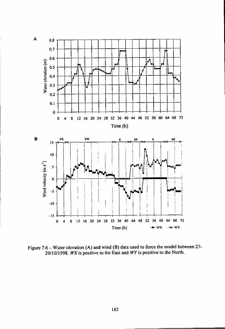
S 0.4
2 0.3
^ 0 . 2
0 4 8 12 16 20 24 28 32 36 40 44 48 52 56 60 64 68 72
Time (h)
B sw
(J
>
0 4 8 12 16 20 24 28 32 36 40 44 48 52 56 60 64 68 72
Time(h) -*-wx -fc-WY
Figure 7.6 - Water elevation (A) and wind (B) data used to force the model between 27-29/10/1998. IVX 'is positive to the East and WY is positive to the North.
162
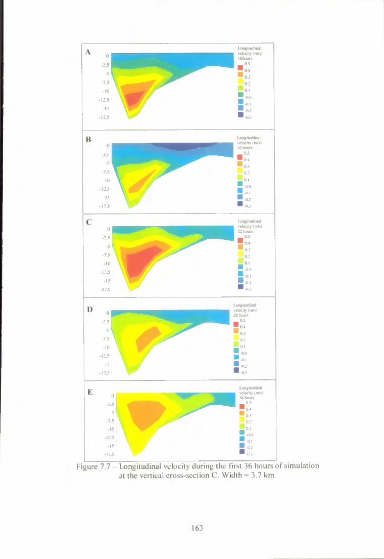
14>ngiiiKlin.il
clocil> (m/M
I t>ni.'iUKlin:il kclocil> (m/si I o h o u r s
17.5
clocity I m/M
velocity (nvM
l . o n ^ M i i H l i i u l
Figure 7.7 - Longitudinal velocity during the first 36 hours of simulation at the vertical cross-section C. Width = 3.7 km.
163
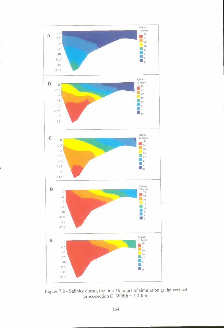
Salinit\
S.ilillil\
SalinilN
SalinilN . 8 ho i irx
Figure 7.8 - Salinity during the first 36 hours of simulation at the vertical cross-section C. Width = 3.7 km.
164
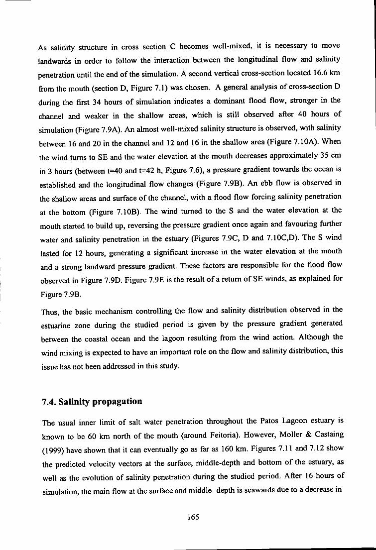
As salinity structure in cross section C becomes well-mixed, it is necessary to move
landwards in order to follow the interaction between the longitudinal flow and salinity
penetration until the end of the simulation. A second vertical cross-section located 16.6 km
from the mouth (section D, Figure 7.1) was chosen. A general analysis of cross-section D
during the first 34 hours of simulation indicates a dominant flood flow, stronger in the
channel and weaker in the shallow areas, which is still observed after 40 hours of
simulation (Figure 7.9A). An almost well-mixed salinity structure is observed, with salinity
between 16 and 20 in the channel and 12 and 16 in the shallow area (Figure 7.10A). When
the wind turns to SE and the water elevation at the mouth decreases approximately 35 cm
in 3 hours (between t=40 and t=42 h. Figure 7.6), a pressure gradient towards the ocean is
established and the longitudinal flow changes (Figure 7.9B). An ebb flow is observed in
the shallow areas and surface of the channel, with a flood flow forcing salinity penetration
at the bottom (Figure 7.1 OB). The wind turned to the S and the water elevation at the
mouth started to build up, reversing the pressure gradient once again and favouring ftirther
water and salinity penetration in the estuary (Figures 7.9C, D and 7.10C,D), The S wind
lasted for 12 hours, generating a significant increase in the water elevation at the mouth
and a strong landward pressure gradient. These factors are responsible for the flood flow
observed in Figure 7,9D. Figure 7.9E is the result of a return of S E winds, as explained for
Figure 7.9B.
Thus, the basic mechanism controlling the flow and salinity distribution observed in the
estuarine zone during the studied period is given by the pressure gradient generated
between the coastal ocean and the lagoon resulting fi-om the wind action. Although the
wind mixing is expected to have an important role on the flow and salinity distribution, this
issue has not been addressed in this study.
7.4. Salinity propagation
The usual inner limit of salt water penetration throughout the Patos Lagoon estuary is
known to be 60 km north of the mouth (around Feitoria). However, MoIIer & Castaing
(1999) have shown that it can eventually go as far as 160 km. Figures 7.11 and 7.12 show
the predicted velocity vectors at the surface, middle-depth and bottom of the estuary, as
well as the evolution of salinity penetration during the studied period. After 16 hoiu^ of
simulation, the main flow at the surface and middle- depth is seawards due to a decrease in
165
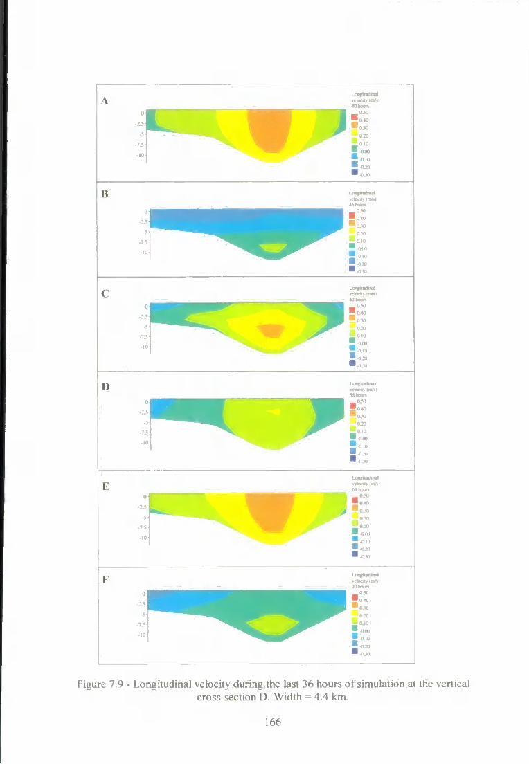
H
0 » 0.40
'OJO 020
^OIO »<ll « lO
1)
OJO O.0
I H I I
« , »
' I I Ml
-5
•10
•ttJO
Figure 7.9 - Longitudinal velocity during the last 36 hours of simulation at the vertical cross-section D. Width = 4.4 km.
166
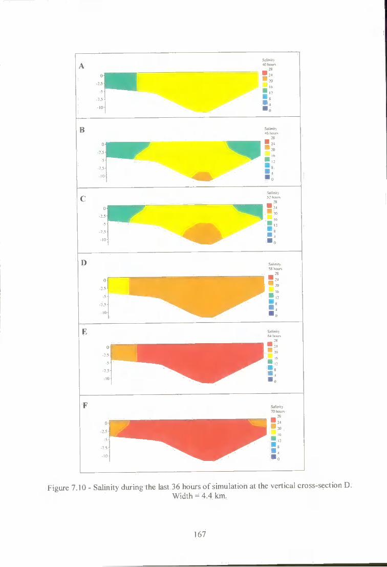
Salmiiv 40houn
!E _ 16
Salini(> 52 houn
• 2 0
SS h ,Hir\
•V-lllllllN
70 h»urv
Figure 7.10 - Salinity during the last 36 hours of simulation at the vertical cross-section D. Width = 4.4 km.
167
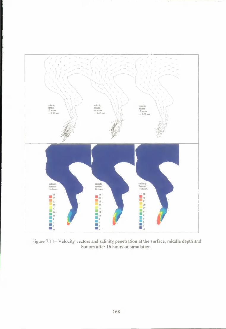
l6houn 0 lOrn^
Figure 7 .11- Velocity vectors and salinity penetration at the surface, middle depth and bottom after 16 hours of simulation.
168
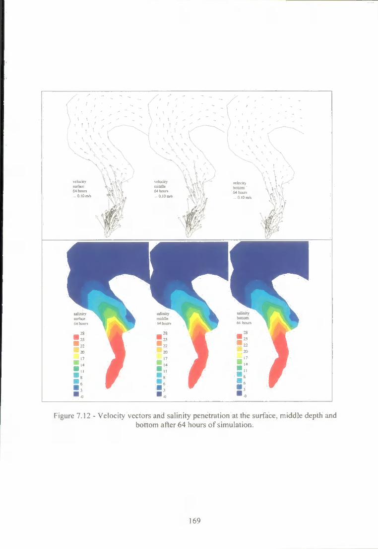
Mhoun 0 .10 m/% 0.10 n / i
Figure 7.12 - Velocity vectors and salinity penetration at the surface, middle depth and bottom after 64 hours of simulation.
169
the water elevation and wind velocity (Figure 7.6), while the flow at the bottom remains
landwards, favouring salt water penetration. Although the salt wedge reaches 5.3 km north
of the mouth at the bottom and 2.2 km at the surface, salinity is observed up to 10.6 km at
the bottom and 9.5 km in the surface (Figure 7.11).
The predominance of SW winds throughout the simulation favoured the continuous
penetration of salt water. The predicted longitudinal salinity distribution after 64 hours of
simulation indicates a homogeneous penetration of the salt wedge 18 km landwards,
although salinity can be observed up to 34 km north of the mouth (Figure 7.12).
Predictions indicate that the salt wedge is penetrating the estuary at a rate of 0.28 km h'*.
7.5. Estuarine mixing
Quantification of mixing processes and rates of turbulent exchange of salt are among the
largest outstanding problems of research in estuaries (Dyer & New, 1986). Mixing in
estuaries is caused by turbulence produced by bottom finction and by internal shear (Dyer,
1982; 1997), which are often assumed to be driven by the tidal force (Goodrich et a/.,
1987), although occasionally the wind mixing can be significant. The balance between
bottom fiiction and internal shear varies, the former being dominant in well-mixed
estuaries, the latter in highly stratified estuaries (Abrahams, 1980). In partially mixed
estuaries both are important.
Dyer & New (1986) describe the mixing mechanism driven by tidal oscillations. It is
believed that a similar mechanism applies for wind-driven systems, assuming that subtidal
oscillations of the whole water mass over the bottom roughness elements and around
topographic irregularities produce turbulence on various scales creating a vertical flux of
momentum which works against the buoyancy forces to progressively break down
stratification. When the velocity shear across the interface between the layers exceeds a
critical value, small instabilities form and grow into waves and eventually break. Dyer
(1997) comments that the form of the instabilities created at the interface depends on the
relative thicknesses of the velocity interface and the density surface, and the relative
position of the centres of the gradient zones. The instabihties thicken the interface,
decrease the gradients of density and velocity, and restabilize the stratification. The major
distinction between them is in terms of the Richardson number, which represents a
comparison of the stabilizing forces of the density stratification to the destablizing
170
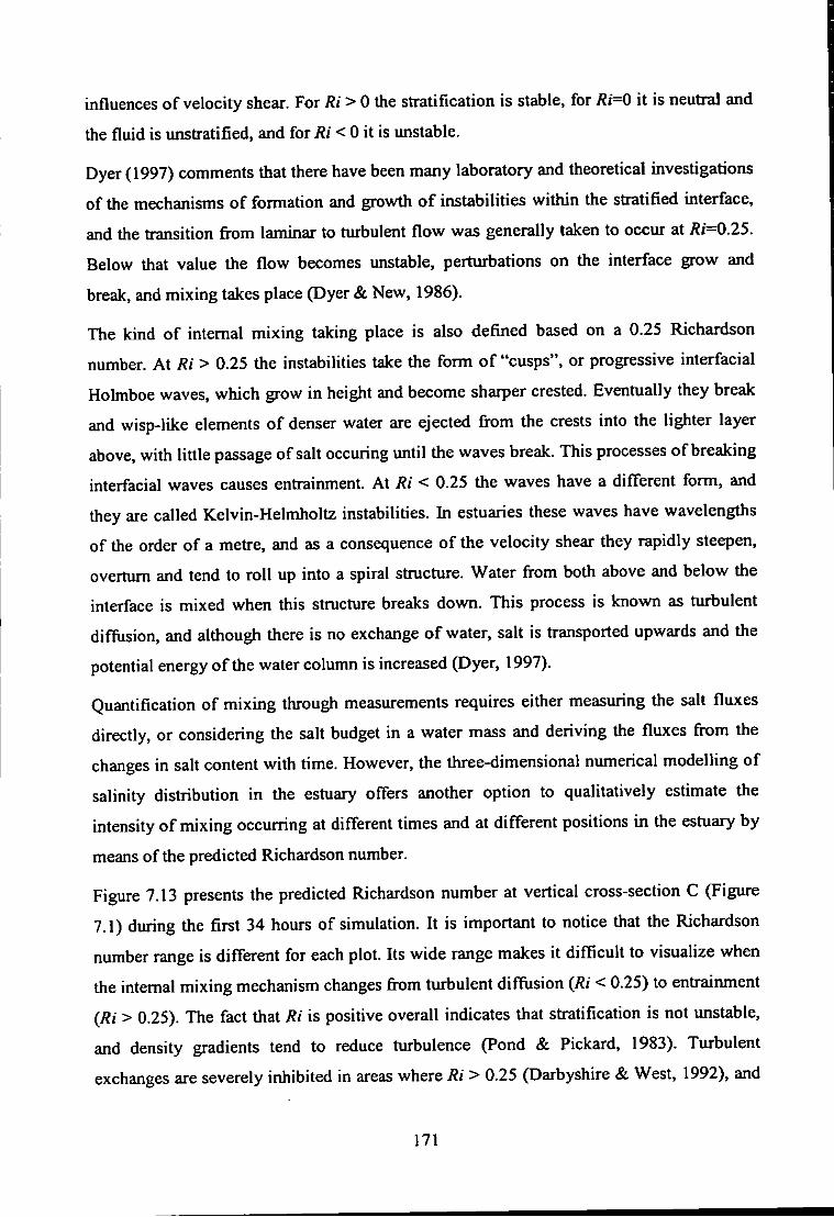
influences of velocity shear. For > 0 the stratification is stable, for Ri=0 it is neutral and
the fluid is unstratified, and for Ri < 0 it is unstable.
Dyer (1997) comments that there have been many laboratory and theoretical investigations
of the mechanisms of formation and growth of instabilities within the stratified interface,
and the transition fi-om laminar to tiu-bulent flow was generally taken to occur at Ri=0.25,
Below that value the flow becomes unstable, perturbations on the interface grow and
break, and mixing takes place (Dyer & New, 1986).
The kind of internal mixing taking place is also defined based on a 0.25 Richardson
number. At Ri > 0.25 the instabilities take the form of "cusps", or progressive interfacial
Holmboe waves, which grow in height and become sharper crested. Eventually they break
and wisp-like elements of denser water are ejected fi^om the crests into the lighter layer
above, with little passage of salt occuring until the waves break. This processes of breaking
interfacial waves causes entrainment. At Ri < 0.25 the waves have a different form, and
they are called Kelvin-Helmholtz instabilities. In estuaries these waves have wavelengths
of the order of a metre, and as a consequence of the velocity shear they rapidly steepen,
overturn and tend to roll up into a spiral structure. Water fi-om both above and below the
interface is mixed when this structiu-e breaks down. This process is known as turbulent
diffusion, and although there is no exchange of water, salt is transported upwards and the
potential energy of the water column is increased (Dyer, 1997).
Quantification of mixing through measurements requires either measuring the salt fluxes
directly, or considering the salt budget in a water mass and deriving the fluxes from the
changes in salt content with time. However, the three-dimensional numerical modelling of
salinity distribution in the estuary offers another option to qualitatively estimate the
intensity of mixing occurring at different times and at different positions in the estuary by
means of the predicted Richardson number.
Figure 7.13 presents the predicted Richardson number at vertical cross-section C (Figure
7.1) during the first 34 hours of simulation. It is important to notice that the Richardson
number range is different for each plot. Its wide range makes it difficult to visualize when
the internal mixing mechanism changes from turbulent diffusion {Ri < 0.25) to entrainment
(Ri > 0.25), The fact that Ri is positive overall indicates that stratification is not unstable,
and density gradients tend to reduce turbulence (Pond & Pickard, 1983). Turbulent
exchanges are severely inhibited in areas where Ri > 0.25 (Darbyshire & West, 1992), and
171
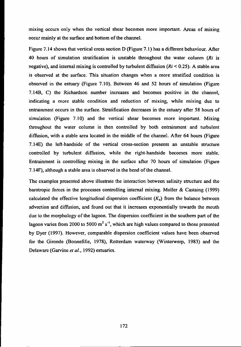
mixing occurs only when the vertical shear becomes more important. Areas of mixing
occur mainly at the surface and bottom of the channel.
Figure 7.14 shows that vertical cross section D (Figure 7.1) has a different behaviour. After
40 hours of simulation stratification is unstable throughout the water colunm (Ri is
negative), and internal mixing is controlled by turbulent diffusion {Ri < 0.25). A stable area
is observed at the surface. This situation changes when a more stratified condition is
observed in the estuary (Figure 7.10). Between 46 and 52 hours of simulation (Figure
7.14B, C) the Richardson number increases and becomes positive in the channel,
indicating a more stable condition and reduction of mixing, while mixing due to
entrainment occurs in the surface. Stratification decreases in the estuary after 58 hours of
simulation (Figure 7.10) and the vertical shear becomes more important. Mixing
throughout the water column is then controlled by both entraimnent and turbulent
diffusion, with a stable area located in the middle of the charmel. After 64 hours (Figure
7.14E) the left-handside of the vertical cross-section presents an unstable structure
controlled by turbulent diffusion, while the right-handside becomes more stable.
Entrainment is controlling mixing in the surface after 70 hours of simulation (Figure
7.14F), although a stable area is observed in the bend of the channel.
The examples presented above illustrate the interaction between salinity structure and the
barotropic forces in the processes controlling internal mixing. Moller & Castaing (1999)
calculated the effective longitudinal dispersion coefficient (Kx) from the balance between
advection and diffusion, and found out that it increases exponentially towards the mouth
due to the morphology of the lagoon. The dispersion coefficient in the southern part of the
lagoon varies fi^om 2000 to 5000 m^ s"\ which are high values compared to those presented
by Dyer (1997). However, comparable dispersion coefficient values have been observed
for the Gironde (BonnefiUe. 1978), Rotterdam waterway (Winterwerp, 1983) and the
Delaware (Garvine et a/., 1992) estuaries.
172
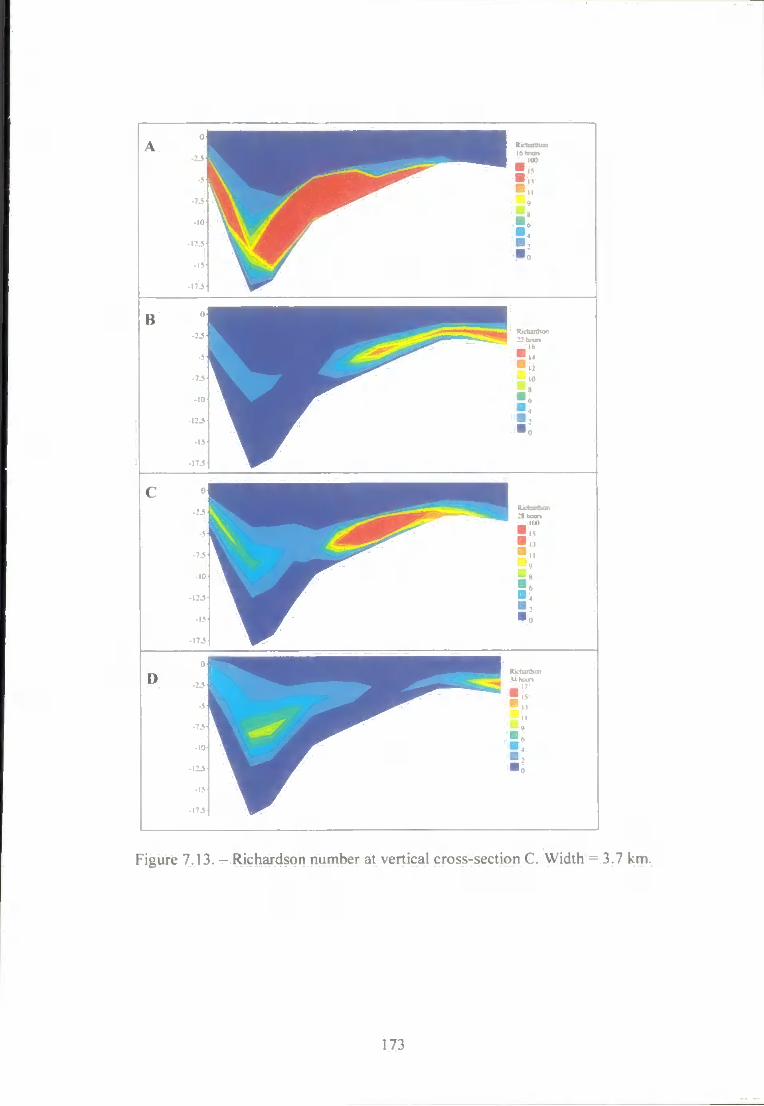
A
• 10'
- I i 5
1 1 6 ioirs
100
' I I
A
• 10'
- I i 5
6 ioirs 100
' I I
-73-
•10
- I 2 J
•15
•113
i lK-h.nK .Mi 12 houn
I I .
' 12
H>
x
J* J:
c "1
J
•73
•10
-123
•15
-173
RtchurKon
* I I
0
J :
oJ I>
• 7 3 '
•10
-123
•15
• 173
1 K k hnun
IS
I f
0
Figure 7.13. - Richardson number at vertical cross-section C. Width = 3.7 km.
173
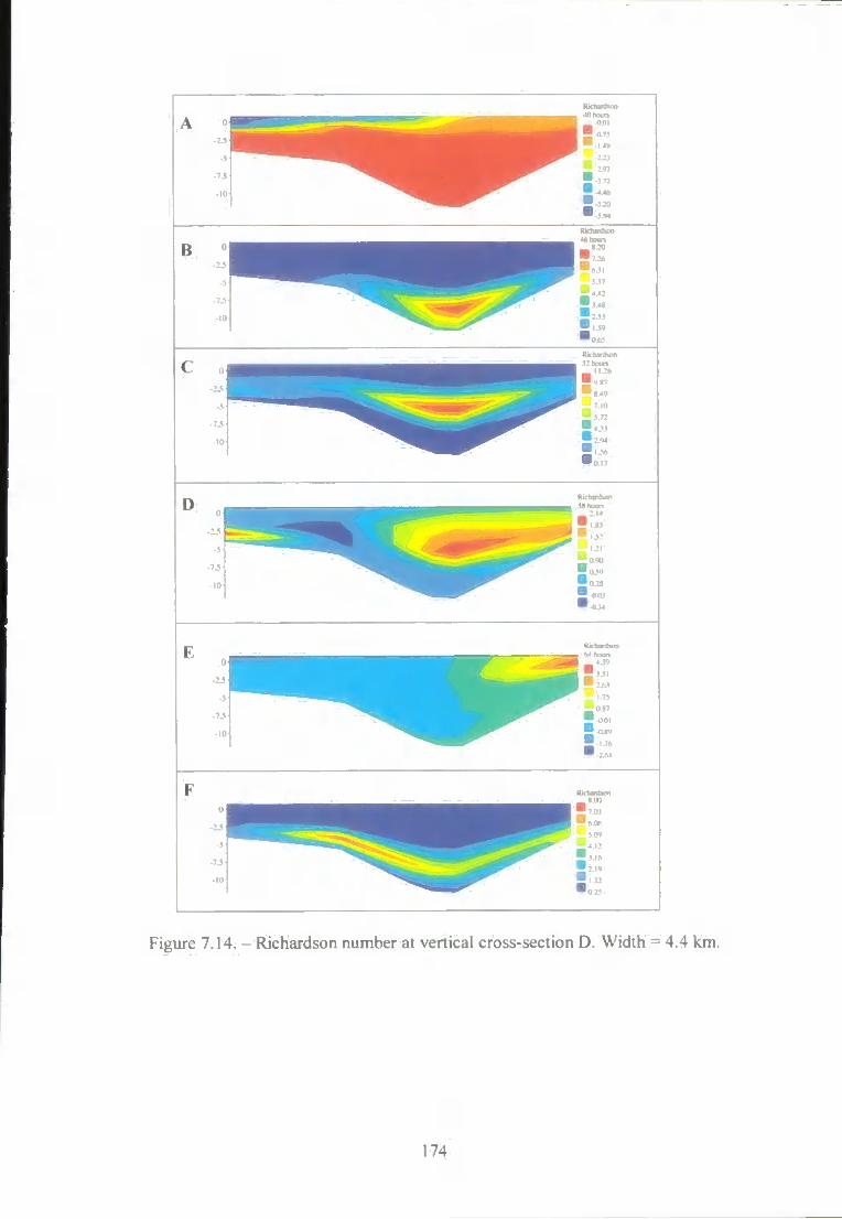
1)
Figure 7.14. - Richardson number at vertical cross-section D. Width = 4.4 km.
174
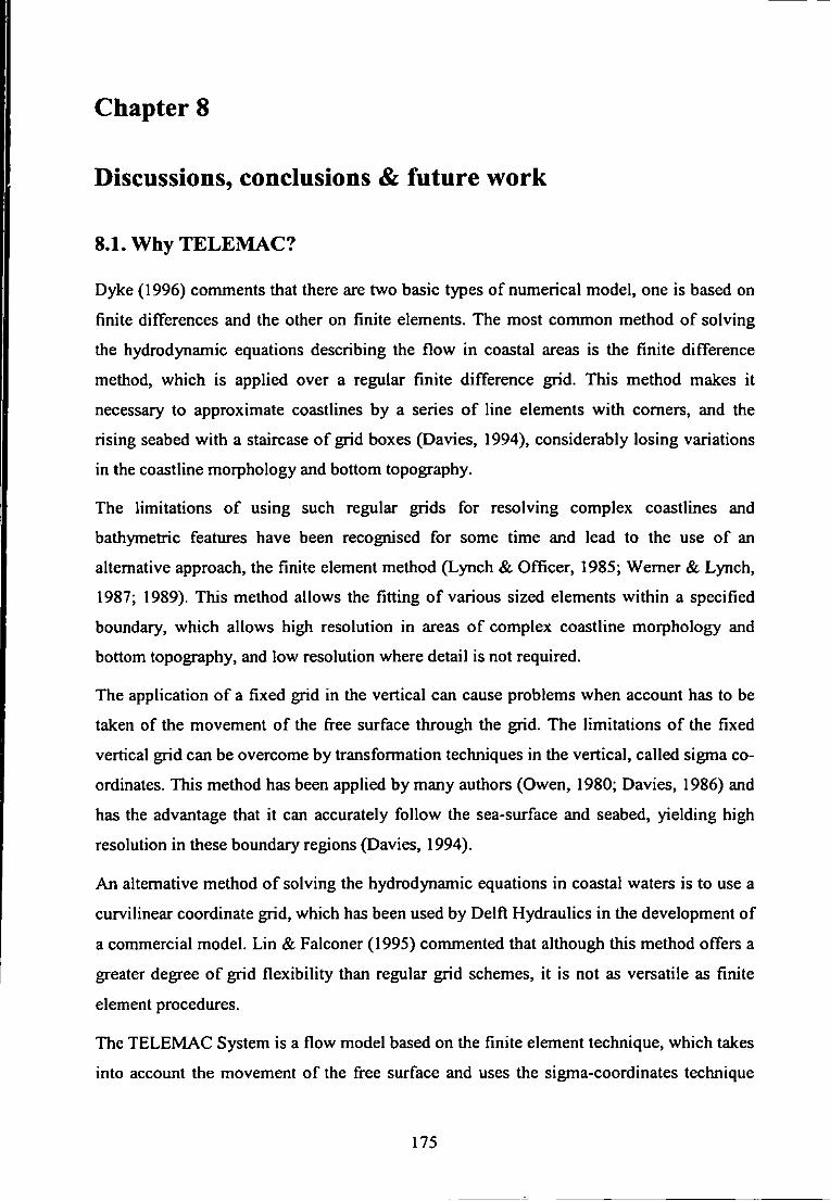
Chapter 8
Discussions, conclusions & future work
8.1. Why TELEMAC?
Dyke (1996) comments that there are two basic types of numerical model, one is based on
finite differences and the other on finite elements. The most common method of solving
the hydrodynamic equations describing the flow in coastal areas is the finite difference
method, which is applied over a regular finite difference grid. This method makes it
necessary to approximate coastlines by a series of line elements with comers, and the
rising seabed with a staircase of grid boxes (Davies, 1994), considerably losing variations
in the coastline morphology and bottom topography.
The limitations of using such regular grids for resolving complex coastlines and
bathymetric features have been recognised for some time and lead to the use of an
alternative approach, the finite element method (Lynch & Officer, 1985; Werner & Lynch,
1987; 1989). This method allows the fitting of various sized elements within a specified
boundary, which allows high resolution in areas of complex coastline morphology and
bottom topography, and low resolution where detail is not required.
The application of a fixed grid in the vertical can cause problems when account has to be
taken of the movement of the fi-ee surface through the grid. The limitations of the fixed
vertical grid can be overcome by transformation techniques in the vertical, called sigma co
ordinates. This method has been applied by many authors (Owen, 1980; Davies, 1986) and
has the advantage that it can accurately follow the sea-surface and seabed, yielding high
resolution in these boundary regions (Davies, 1994).
An alternative method of solving the hydrodynamic equations in coastal waters is to use a
curvilinear coordinate grid, which has been used by Delfl Hydraulics in the development of
a commercial model. Lin & Falconer (1995) commented that although this method offers a
greater degree of grid flexibility than regular grid schemes, it is not as versatile as finite
element procedures.
The T E L E M A C System is a flow model based on the finite element technique, which takes
into account the movement of the fi-ee surface and uses the sigma-coordinates technique
175
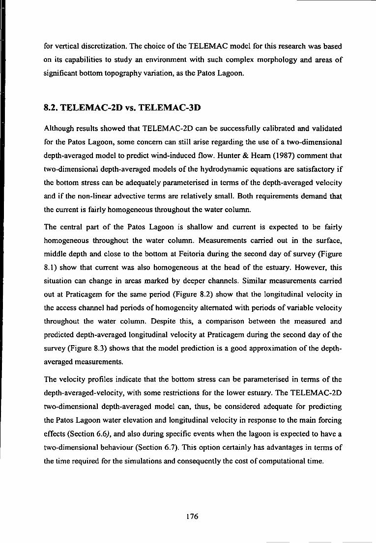
for vertical discretization. The choice of the TELEMAC model for this research was based
on its capabilities to study an environment with such complex morphology and areas of
significant bottom topography variation, as the Patos Lagoon.
8.2. TELEMAC-2D vs. TELEMAC-3D
Although results showed that TELEMAC-2D can be successfully calibrated and validated
for the Patos Lagoon, some concern can still arise regarding the use of a two-dimensional
depth-averaged model to predict wind-induced flow. Hunter & Heam (1987) comment that
two-dimensional depth-averaged models of the hydrodynamic equations are satisfactory i f
the bottom stress can be adequately parameterised in terms of the depth-averaged velocity
and i f the non-linear advective terms are relatively small. Both requirements demand that
the current is fairly homogeneous throughout the water column.
The central part of the Patos Lagoon is shallow and current is expected to be fairly
homogeneous throughout the water column. Measurements carried out in the surface,
middle depth and close to the bottom at Feitoria during the second day of survey (Figure
8.1) show that current was also homogeneous at the head of the estuary. However, this
situation can change in areas marked by deeper channels. Similar measurements carried
out at Praticagem for the same period (Figure 8.2) show that the longitudinal velocity in
the access channel had periods of homogeneity alternated with periods of variable velocity
throughout the water column. Despite this, a comparison between the measured and
predicted depth-averaged longitudinal velocity at Praticagem during the second day of the
survey (Figure 8.3) shows that the model prediction is a good approximation of the depth-
averaged measurements.
The velocity profiles indicate that the bottom stress can be parameterised in terms of the
depth-averaged-velocity, with some restrictions for the lower estuary. The TELEMAC-2D
two-dimensional depth-averaged model can, thus, be considered adequate for predicting
the Patos Lagoon water elevation and longitudinal velocity in response to the main forcing
effects (Section 6,6), and also during specific events when the lagoon is expected to have a
two-dimensional behaviour (Section 6.7). This option certainly has advantages in terms of
the time required for the simulations and consequently the cost of computational time.
176
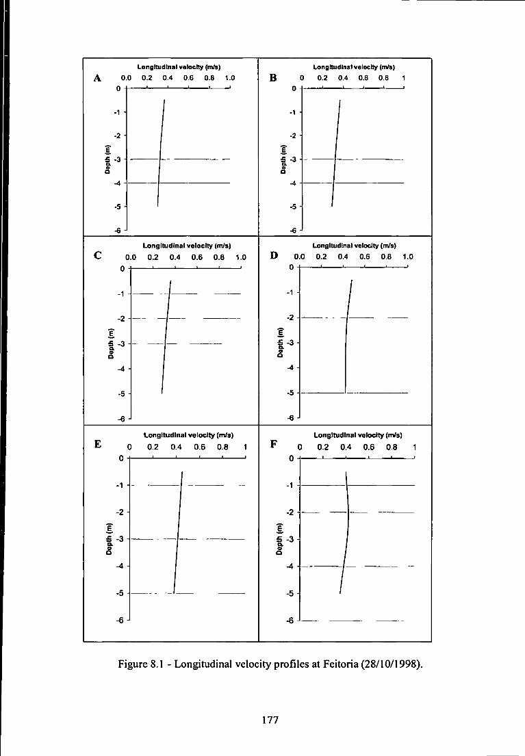
Longitudinal valocity (m/s) A 0.0 0.2 0.4 0.6 0.8 1.0
-1 H
E
t-3
-5
B Longitudinal vQloctty (m/s)
0 0.2 0.4 0.6 0.8 1
-2
? t-3
Longitudinal velocity (m/s) C 0.0 0.2 0.4 0.6 0.8 1.0
Longitudinal velocity (nVs) D 0.0 0.2 0.4 0.6 0.8 1.0
•1 H
-2
t-3
•1 H
E
i - 3
E Longitudinal velocity (m/s)
0 0.2 0.4 0.6 0.8 1
a &
-1
-2H
-3
-A H
-5
-6
Longitudinal velocity (m/s) F 0 0.2 0.4 0.6 0.8 1
0
Figure 8.1 - Longitudinal velocity profiles at Feitoria (28/10/1998).
177
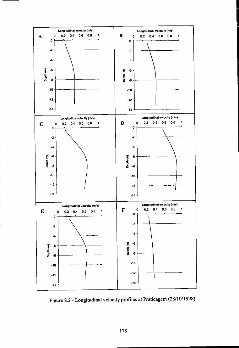
Longitudinal veloelly (m/s)
0 0.2 0.4 0.6 0.8 1
0
-2
-4
I ^ I -a
-10
-12
-14
Longitudinal Velocity (m/s)
B 0 0.2 0.4 0.6 0.8 1
0
Longitudinal velocity {mis)
Q 0 0.2 0.4 0.6 0.8 1 0
-2
-4
I ^ f -8
-10
-12
-14
Longitudinal velocity (m/s)
0 0.2 0.4 0.6 0.8 1
-6
-8
-10
•12-1
-14
Longitudinal velocity (m/s)
0 0.2 0.4 0.6 0.8 1
Longitudinal velocity (m/a)
0 0.2 0.4 0.6 0.8 1
0
-2
-4
? -6
a, a -a
10 H
•12
-14
-4 H
-6
-8
-10
-12
-14
Figure 8.2 - Longitudinal velocity profiles at Praticagem (28/10/1998),
178
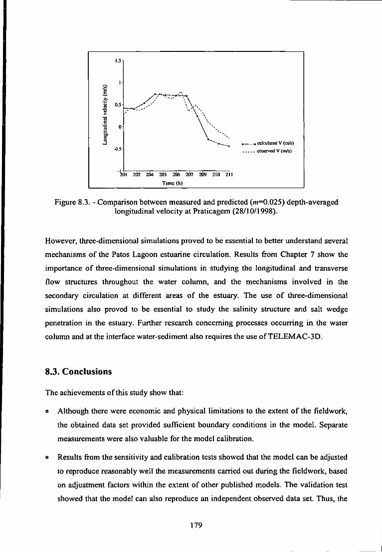
1 •g 0.5
-0.5 , calculated V (m/s)
obsoved V (nVs)
' io i 202 204 205 206 207 209 210 211
Time (h)
Figure 8.3. - Comparison between measured and predicted (/w=0.025) depth-averaged longitudinal velocity at Praticagem (28/10/1998).
However, three-dimensional simulations proved to be essential to better understand several
mechanisms of the Patos Lagoon estuarine circulation. Results from Chapter 7 show the
importance of three-dimensional simulations in studying the longitudinal and transverse
flow structures throughout the water column, and the mechanisms involved in the
secondary circulation at different areas of the estuary. The use of three-dimensional
simulations also proved to be essential to study the salinity structure and salt wedge
penetration in the estuary. Further research concerning processes occurring in the water
column and at the interface water-sediment also requires the use of TELEMAC-3D.
8.3. Conclusions
The achievements of this study show that:
o Although there were economic and physical limitations to the extent of the fieldwork,
the obtained data set provided sufficient boundary conditions in the model. Separate
measurements were also valuable for the model calibration.
o Results from the sensitivity and calibration tests showed that the model can be adjusted
to reproduce reasonably well the measurements carried out during the fieldwork, based
on adjustment factors within the extent of other published models. The validation test
showed that the model can also reproduce an independent observed data set. Thus, the
179
TELEMAC-2D model for the Patos Lagoon is considered successfully calibrated and
validated, and can then be used as a predictive tool to study the Patos Lagoon
circulation.
The main forces controlling the Patos Lagoon subtidal circulation proved to be the
barotropic pressure gradients established between the lagoon and the coastal area as a
result of the local and remote wind effect, modulated by the passage of fi-ontal systems
over the area, and the freshwater discharge.
• The local wind acts inside the lagoon through the set-up/set-down mechanism
of oscillation, as i f the lagoon was a closed basin.
• The non-local wind acts in the coastal area and drives the circulation in the
lower estuary. This causes considerable exchange of water between the
estuarine part of the lagoon and the sea.
• The river discharge controls the water elevation inside the lagoon and the
direction of the pressure gradient established within the estuary. A riverine
inflow of 2500 m** s' is required to maintain the lagoon water level at its
present mean elevation.
The entrance channel of the Patos Lagoon works as a filter and strongly reduces the
tidal and subtidal oscillations generated offshore. Estimates of the tidal attenuation
indicate that the diurnal and semi-diurnal tidal signals are similarly attenuated, while
the quarter-diurnal signal penetrates further in the lagoon. Estimates indicate that the
subtidal energy propagates further inland.
Predictions of the Patos Lagoon behaviour during an El Nifio event indicate that:
• The lagoon residence time is a function of the freshwater inflow, varying from
135 to 68 days for an inflow of 5000 and 10000 m^ s\ respectively.
• The non-local forcing dominates the water exchanges between the lagoon and
the adjacent coastal area. Approximately 7% of the lagoon volume can be
moved into or out in time intervals as small as 6 hours. The outflow of water
dominates the inflow, illustrating the lagoon's long-term seaward residual flow.
• The stronger the discharge at the top of the lagoon the stronger the pressure
gradient towards the ocean and the outflow of water, and longer the time
180
required for the non-local effects to reverse the pressure gradient landwards and
force water into the lagoon.
• Three-dimensional simulations of the longitudinal and transverse flows illustrate the
different forces controlling two areas of the estuary.
• At the top of the estuary (Feitoria) the longitudinal flow is mainly controlled by
the pressure gradients generated through the set-up/set-down mechanism of
oscillation due to the local wind effect. The transverse flow in the shallow areas
is modulated by the wind and remains in the downwind direction, while lateral
pressure gradients drive the transverse flow in the deeper areas.
• At the lower estuary (SJN) the longitudinal flow is controlled by the non-local
effect represented by the water elevation at the ocean boundary. The transverse
flow results fi^om the interaction between the longitudinal flow and the channel
curvature and geometry.
• Three-dimensional simulations indicate that the basic mechanism controlling the
advection of salt water into the estuary and the vertical salinity structure varying from
stratified to well-mixed is the barotropic pressure gradient between the lagoon and the
coast due to the wind. Estimates of the salt wedge penetration indicate a rate of 0.28
kmhV
• The use of the Richardson number was explored as an indicator of the estuarine mixing
during the studied period. When the estuary presents a high degree of stratification the
Richardson number increases and turbulence and mixing are reduced. When the estuary
is less stratified the vertical shear becomes more important breaking the stability of the
salinity structure and favouring mixing due to entrainment and turbulent diffusion. The
distribution of the Richardson number shows that mixing occurs mainly at the surface
and bottom of the channel, while more stable conditions tend to occur where
stratification is dominant.
• The use of TELEMAC-2D to study the Patos Lagoon two-dimensional depth-averaged
circulation during the period when fieldwork was carried out in the estuary proved to
be a valuable tool for future predictions of the main forcing effects. The use of
TELEMAC-3D for the same period complements the knowledge about the flow and
salinity structures throughout the water column and gives an idea about their
interaction with the barotropic forces.
181
8.4. Future Work
Based on the difficulties observed throughout the project and also the possibilities offered
by the TELEMAC model, this project comes to an end leaving several suggestions for
future work and improvements.
The major deficiency to be improved before fiirther developments in the model is the lack
of river discharge time series at the top of the lagoon. Such measurements are essential to
better predict the freshwater influence in the Patos Lagoon circulation.
Measurements of continuous time series of wind, water elevation and velocities at different
locations throughout the lagoon and estuarine area would also be recommended.
Measurements at the mouth of the estuary would provide data to be used as boundary
conditions in longer simulations, while measurements inside the lagoon and estuary could
be used as a reference for model validation. Measurements throughout the water column
would also be recommended to better represent the three-dimensional features of the
boundary conditions, especially regarding the salinity and suspended sediment structures.
The magnitude of evaporation over such a huge lagoon is certainly important, especially
during the summer months. Although this is expected to affect the volume of water
exchanged between the lagoon and the coastal area, and also the estuarine salt balance, it
was not taken into account in the present study. Evaporation is, thus, an important issue to
be included in future modelling experiments.
In three-dimensional simulations, further plots of consecutive vertical cross-sections
perpendicular to the main flow direction can give a better description of the secondary flow
throughout the lagoon and the estuarine area. The interaction between the secondary flow
and salinity stratification also deserves special attention.
Further three-dimensional simulations based on the appropriate boundary conditions are
recommended to better understand several aspects of the Patos Lagoon baroclinic
circulation. Numerical simulations can be used to study in more detail the interaction
between the subtidal flow, density-induced flow and bathymetry in establishing the
longitudinal and transverse circulation in the estuary. On the other hand, longer simulations
can be used to study the effect of the passage of weather fronts on the estuarine mixing and
on the vertical and horizontal salinity structures. The seasonal variation of the lagoon
baroclinic circulation can also be addressed.
182
Incorporating the sediment transport module (SEDI3D) in the three-dimensional
hydrodynamic module to account for the specific features of cohesive sediments is the next
step forward. The SEDI3D module accounts for processes related to suspended sediment
transport, including settling velocity and modelling of the turbulence and buoyancy effects,
processes of erosion occurring at the water-sediment interface and the consolidation
process of the bed. Such features will be valuable in studying the distribution of suspended
sediment in the lagoon, identifying areas of erosion and deposition, and also the position of
the turbidity maximum in the estuary.
The knowledge of the sediment transport processes in the lagoon is of great social and
economical importance for the region, as several studies concerning Rio Grande Harbour,
the water quality and the lagoon management can be addressed. Further three-dimensional
simulations can, for example, illustrate the effect that widening and/or deepening the
estuary access channel will have on currents, water elevation, residence time, salt water
penetration and suspended sediment behaviour. Other important issues as harbour siltation,
and minimisation of dredging and dredging disposal via sediment management can also
benefit fi^om the association between the hydrodynamic and sediment transport modules.
183
References Abrahams, G. 1980. On internally generated estuarine turbulence. 1:344-1:353. Trondheim. Proc. 2"** Int. Symp. Stratified Flows.
Aldridge, J. N. & Davies, A. M. 1993. A high-resolution three-dimensional hydrodynamic tidal model of the Eastern Irish Sea. Journal of Physical Oceanography 23, 207-224.
Almeida, M. T, A., Baumgarten, M. G. Z. & Rodrigues, R. M . S. 1993. Identificapao das possiveis fontes de contamina9ao das aguas que margeiam a cidade de Rio Grande. Documentos Tecnicos em Oceanografia, N^6, Funda9ao Universidade Federal do Rio Grande, Brazil.
Argyris, J. H. & Kelsey, S. 1960. Energy theorems and structural analysis. Butterworth, London. Collection of papers published in Aircr. Eng., 1954 and 1955.
Asmus, M. L. 1997. Coastal Plain and Patos Lagoon. In: Subtropical Convergence Environments ~ The Coast and Sea in the Southwestern Atlantic. Eds. U. Seeliger, C. Odebrecht, and J. P. Castello. pp. 9-12. Springer Veriag.
Baisch, P. R., Jouanneau, J. M. & Asmus, H. E. 1989. Chemical composition of sediments from the Patos Lagoon. Xin Int. Geoch. Expl. Symp n Braz. Geoch. Cong., pp 11-20
Barnes, R. S. K. 1980. Coastal Lagoons. Cambridge University Press.
Bates, P. D., Anderson. M. G., Price. D. A., Hardy, R. J., & Smith, C. N. 1996. Analysis and development of hydraulic models for floodplain flows. In: Floodplain Processes. Eds. M. G. Anderson, D. E. Walling, and P. D. Bates, pp. 215-254.
Bates, P. D., Anderson, M . G., Hervouet, J. M. , & Hawkes, J. C. 1997. Investigating the behaviour of two-dimensional finite element models of compound channel flow. Earth Surface Processes and Landforms 22, 3-17.
Bates, P. D., Horrit, M., & Hervouet, J. M. 1998. Investigating two-dimensional, finite element predictions of floodplain inundation using fractal generated topography. Hyrological Processes n, 1257-1277.
Bathurst, J. C, Thome, C. R., & Hey, R. D. 1977. Direct measurements of secondary flows in river bends. Nature 269, 504-506.
Bicalho, A. 1883. Relat6rio da Comissao de melhoramentos da Barra do Rio Grande. Obras do Porto e da Barra do Rio Grande do Sul. Oficina Grafica da Federa^So, Vol. 3.
Bird, E. C. F. 1967. Coastal lagoons of south-eastern Australia. In: Landform Studies from Australia and New Guinea. Eds. J, N. Jennings and J. A. Mabbutt. pp. 365-385.
184
Bird, E. C. F. 1994. Physical setting and geomorphology of coastal lagoons. In: Coastal Lagoon Processes. Ed. B. Kjerfve. pp. 9-39. Elsevier,
Blain, C. A., Westerink, J. J., & Luettich, R. A. 1994. The influence of domain size on the response characteristics of a hurricane storm surge model. Journal of Geophysical Research 99, 18467-18479.
Bonnefille, R. 1978. Residual phenomena in estuaries, application to the Gironde estuary. In: Hydrodynamics of Estuaries and Fjords. Ed. J. C. J. Nihoul. pp. 439-482.
Bordas, M . P., Casalas, A., Silveira, A., & Gon^alves, M . 1984. Circula^ao e dispersao em sistemas costeiros e oceanicos. Caso da Lagoa dos Patos. Technical Report, Instituto de Pesquisas Hidraulicas da Universidade Federal do Rio Grande do Sul, Porto Alegre, Brasil.
Brenon, I . & Le Hir, P. 1999, Modelling the turbidity maximum in the Seine estuary (France): identification of formation processes. Estuarine, Coastal and Shelf Science 49, 525-544.
Brooks, A. N. & Hughes, T. J. R, 1982. Streamline Upwind/Petrov-Galerkin formulations for convection dominated flows with particular emphasis on the incompressible Navier-Stokes Equations. Computer Methods in Applied Mechanics and Engineering 32, 199-259.
Bruun, P. 1994. Engineering projects in coastal lagoons. In: Coastal Lagoon Processes. Ed. B. Kjerfve. pp. 507-533. Elsevier
Butt, T. 1999. Sediment transport in the swash-zone of natural beaches. PhD Thesis, Institute of Marine Studies, University of Plymouth, UK.
Calliari, L. J. 1980. Aspectos sedimentol6gicos e ambientais na regiSo estuarial da Laguna dos Patos. MSc Dissertation, Universidade Federal do Rio Grande do Sul, Brazil
Calliari, L. J. & Facchin, S. 1993. Laguna dos Patos: Influencia nos depositos laminicos costeiros. Pesquisas 20, 57-69.
Calliari, L. J. 1997. Environment and Biota of the Patos Lagoon. In: Subtropical Convergence Environments - The Coast and Sea in the Southwestern Atlantic. Eds. U. Seeliger, C. Odebrecht, and J. P. Castello. pp. 13-18. Springer Veriag.
Castanares, A. & Phleger. F. B. 1969. Lagunas Costeras, un Simposio, UNAM-UNESCO. Mexico.
Castelao, R. M. (1999). Estudo da dinamica da Lagoa dos Patos atraves da modelagem numerica. MSc. Dissertation. Funda9ao Universidade Federal do Rio Grande, Brazil.
Castello, J. P. & Moller, O. O. 1977, On the oceanographic conditions in the Rio Grande do Sul State. Atldntica 2, 25-110.
Castello, J. P. & Moller, O. O. 1978. On the relationship between rainfall amd shrimp production in the estuary of Patos Lagoon (RS,Bra2il). Atldntica 3, 67-74.
185
Castello, J. P. 1985. La ecologia de los consumidores del estuario de la Lagoa dos Patos, Brasil. In: Fish Community Ecology in Estuaries and Coastal Lagoons: Towards an ecosystem integration. Ed. A. Yanes-Arancibia. pp. 386-406. DR(N) UNAN Press, Mexico.
Cheng, R, T. 1978. Modelling of hydraulic systems by finite element methods. In: Advances in Hydroscience, Vol. 11. Ed. V. T. Chow. pp. 207-284. Academic Press.
Cheng, R. T. & Walters, R. A. 1982. Modelling of estuarine hydrodynamics and field data requirements. In: Finite Elements in Fluids, Vol. 4. Eds. R. H. Gallagher, D. H. Norrie, J. T. Oden, and O. C. Zienkiewicz. pp. 89-108. John Wiley & Sons.
Cheng, R. T., Burau, J. R. & Gartner, J. W. 1991. Interfacing data analysis and numerical modeling for tidal hydrodynamic phenomena. In: Tidal Hydrodynamics. Ed. B. B. Parker, pp. 201-219. John Wiley and Sons.
Cheng, R. T., Casulli, V. & Gartner, J. W. 1993. Tidal, residual, intertidal mudflat (TRIM) Model and its applications to San Francisco Bay, California. Estuarine, Coastal and Shelf Science 36, 235-2m
Cheng, S. I . 1970. Numerical integration of the Navier-Stokes equations. AIAA 71 8, 2115-2122.
Ciotti, A. M., Odebrecht, C, Filbnann, G. & MoUer, O. O. 1995. Freshwater outflow and subtropical convergence influence on phytoplankton biomass on the southern brazilian continental shelf Continental Shelf Research 15 (14), 1737-1756.
Costa, C. S. B. & Kinas, P. G. 1988. The effect of wind velocity and direction on the salinity regime in the Lower Patos Lagoon estuary. Ciencia e Cultura 40 (9), 909-912.
Csanady, G. T. 1973. Wind-Induced barotropic motions in long lakes. Journal of Physical Oceanography 3, 429-438.
Csanady, G. T. 1982. Circidation in the Coastal Ocean. D. Reidel Publishing Company.
Cucalon, E. 1987. Oceanographic variability off Ecuador associated with an El Nifio event. Journal of Geophysical Research 92, 14,309-14,322.
Darbyshire, E. J. & West, J. R. 1992. Turbulence and shear induced mixing processes in estuaries. In: Dynamics and Exchanges in Estuaries and the Coastal Zone. Ed. D. Prandle. pp. 75-99. American Geophysical Society.
Davies, A. M. 1986. A three-dimensional model of the northwest european continental shelf, with application to the M4 tide. Journal of Physical Oceanography 16, 797-813.
Davies, A. M. 1994. Quasi-three-dimensional models using mixed finite-difference and spectral models. In: Coastal Estuarial and Harbour Engineers Reference Book. Eds. M. B. Abbott and W. A. Price, pp. 117-128. E&FN SPON.
186
Davis, J. C. 1973. Statistics and Data Analysis in Geology, John Wiley & Sons.
De Lacerda, L. D. 1994. Biogeochemistry of heavy metals in coastal lagoons. In: Coastal Lagoon Processes. Ed. B. Kjerfve. pp. 221-241. Elsevier.
Defant, F. 1961. Physical Oceanography, Volume II. Pergamon Press.
Delaney, P. 1965. Fisiografia e geologia de superficie da plamcie costeira do Rio Grande do Sul. Publica^ao Especial da Escola de Geologia da UFRGS, vol 6, pp 1-105.
Dillenburg, S. R. & Toldo, E. E. 2001. Swash bar migration at the inlet of the Lagoa dos Patos Lagoon, Brazil. Journal of Coastal Research, in press.
DNPVN. 1941. Enchentes de maio de 1941. Diretoria Nacional de Portos e Vias de Navega^ao. Porto Alegre, Brazil.
Dyer, K. R. 1977. Lateral circulation effects in estuaries. In: Estuaries, Geophysics and the Environment, pp. 22-28. National Academy of Sciences, Washington DC.
Dyer, K. R. 1982. Mixing caused by lateral internal seiching within a partially mixed estuary. Estuarine, Coastal and Shelf Science 15, 443-457.
Dyer, K. R. & New, A. L. 1986. Intemiittency in estuarine mixing. In: Estuarine variability. Ed. D. A. Wolfe, pp. 321-339.
Dyer, K. R. 1997. Estuaries. John Wiley & Sons, 195 pp.
Dyke, P. 1996. Modelling Marine Processes. Prentice Hall, 158 pp..
Eguiguren, V. 1894. Las lluvias en Piura. Bol.Soc.Geogr.Lima 4, 241-258.
Elliot, A. J. & Wang, D. P. 1978. The effect of meteorological forcing on Chesapeake Bay: the coupling between an estuary system and its adjacent waters. In: Hydrodynamics of Estuaries and Fjords. Ed. J. C. J. Nihoul. pp. 127-145.
Elston, S. A., Blanton, J. O. & Seim, H. E. 2000. Secondary circulation in curved and straight estuarine reaches. 10th International Biennial Conference on Physics of Estuaries and Coastal Seas, 7-11 October 2000, Norfolk, Virginia, USA. pp 172-175.
Femandes, E. H. L. 1997. Modelagem do Transporte de Elementos Particulados e Dissolvidos entre a Regiao Estuarina da Lagoa dos Patos e o Oceano Atlantico. MSc Dissertation, Funda^ao Universidade Federal do Rio Grande.
Femandes, E. H. L. & Niencheski, L. F. H. 1998. Um modelo de caixas simplificado para o estudo dos processos de transporte na regi|o estuarina da Lagoa dos Patos (RS-Brasil). Atlantica 20, 73-85.
Femandes, E. H. L., Dyer, K. R. & Moller, O. O. 2001. On the hydrodynamics of the world's largest choked coastal lagoon: Patos Lagoon (Brazil). Estuaries, in press.
187
Femandes, E. H. L., Dyer, K. R., & Niencheski, L. F. H. 2001. TELEMAC-2D calibration and validation to the hydrodynamics of the Patos Lagoon (Brazil). Journal of Coastal Research, in press.
Femandes, E. H. L., Dyer, K. R., Moller, O. O. & Niencheski, L. F. H. 2001. The Patos Lagoon hydrodynamics during an El Nino event (1998). Continental Shelf Research, in press.
Fetter, A. F. 1999. Estudo da Circula^ao e Processos de Mistura da Lagoa dos Patos Atraves do Modelo de Circula9ao Oceanica da Universidade de Princeton (POM). MSc Dissertation, Funda^ao Universidade Federal do Rio Grande, Brazil.
Fischer, H. B. 1972. Mass transport mechanisms in partially stratified estuaries. Journal of Fluid Mechanics 53, 671-687.
Fischer, H. B. 1976. Mixing and dispersion in estuaries. Ann.Rev.Fluid Mechanics 8, 107-133.
Fisher, R. L. 1955. Cuspate spits of St. Lawrence Island, Alaska. Journal of Geology 63, 133-142.
Fix, G. J. 1975. Finite element models for ocean circulation problems. SIAM Journal of Applied Mathematics 29, 387.
Foreman. M. G. G. & Walters, R. A. 1990. A finite element tidal model for the southwest coast of Vancouver Island. Journal of Computational Physics 52, 290-312.
Foreman, M. G. G., Baptista, A. M., & Walters, R. A. 1992. Tidal model studies of particle trajectories around a shallow coastal bank. Atmosphere-Ocean 30, 43-69.
Foreman, M. G. G., Thomson, R. E., Lynch. D. R. & Walters. R. A. 1992. A finite element model for three-dimensional flows along the west coast os Vancouver Island. Estuarine and Coastal Modelling, Proceedings of the 2" International Conference, pp 574-585.
Gafr^e, C. L. 1927. Relatorio Tecnico da Barra do Rio Grande, dirigido a Inspetoria de Portos. Rios e Canais.
Galland. J. C. Goutal, N. & Hervouet, J. M. 1991. TELEMAC: A new numerical model for solving shallow water equations. Adv. Water Resources 14(3). 138-148.
Gan, M. A. 1992. Ciclogenese e ciclones sobre a America do Sul. PhD. Thesis. Instituto Nacional de Pesquisas Espaciais, Sio Jos dos Campos, Brazil.
Garcia, C. A. E. 1997. Hydrographic Charcateristics. In: Subtropical Convergence Environments - The Coast and Sea in the Southwestern Atlantic. Eds. U. Seeliger. C. Odebrecht, and J. P. Castello. pp. 18-20. Springer Vedag.
Garvine, R. W., McCarthy, R. W. & Wong, K. C. 1992. The axial salinity distribution in the Delaware estuary. Estuarine, Coastal and Shelf Science 35, 157-162.
188
Glen, N. C. 1979. Tidal Measurement. In: Estuarine Hydrography and Sedimentation. Ed, K. R. Dyer. pp. 19-40. Cambridge University Press.
Gomes, A., Tricart, J, L. F. & Trautmann, J, 1987. Estudo ecodinamico da Estagao Ecologica do Taim e seus arredores. Editora da Universidade Federal do Rio Grande do Sul, Porto Alegre, Brazil.
Goodrich, D. M. , Boicourt, W, C, Hamilton. P. & Pritchard, D. W. 1987. Wind-induced destratification in Chesapeake Bay. Journal of Physical Oceanography 17, 2232-2240.
Gray, W. & Pinder, G. 1976. On the relationship between the finite element and finite difference methods. International Journal for Numerical Methods in Engineering 10, 893-923.
Greenberg, D. A., Loder, J. W., Shen, Y., Lynch. D. R., & Naimie, C. E. 1997. Spatial and Temporal structure of the barotropic response of the Scotian Shelf and Gulf of Maine to surface wind stress: A model-based study. Journal of Geophysical Research 102 (C9), 20,897-20,915.
Gross, M. G., Karweit, M., Cronin, W. B. & Schubel, J. R. 1978. Suspended sediment discharge of the Susquehanna river to northern Chesapeake Bay, 1966 to 1976. Estuaries 1, 106-110.
Grotkop, G. 1973. Finite element analysis of long-period water waves. Computer Methods in Applied Mechanics and Engineering 2. 147-ff.
Guilcher, A. 1981. Les etangs littoraux: azonalite d'ensemble et modalites zonales. Bulletin de la Societe Languedocienne de Geographie 15. 3-10.
Haidvogel, D. B., Robinson, A. R. & Schulman, E. E. 1980, The accuracy, efficiency, and stability of three numerical models with application to open ocean problems. Journal of Computational Physics 34, 1-53.
Heam, C. J., Lukatelich, R. J. & Hunter, J, R, 1986. Dynamical models of the Peel-Harvey estuarine system. Environmental Dynamics Report. ED-86-152. The University of western Australia, Nedlands 6009, Western Australia.
Heam, C. J. & Hunter, J. R. 1987. Modelling wind-driven flow in shallow systems on the southwest Australian coast. In: Numerical Modelling: Applications to Marine Systems. Ed. J. Noye. pp. 47-57. Elsevier Science.
Heam, C. J., Lukatelich, R. J. & McComb. A, J. 1994. Coastal lagoon ecosystem modelling. In: Coastal Lagoon Processes. Ed. B. Kjerfve. pp. 471-506. Elsevier.
Hervouet, J. M. 1993. Validating the numerical simulation of dam-breaks and floods. Advances in hydroscience and engineering 1, 754-761.
189
Hervouet, J. M, & Janin, J. M. 1994. Finite element algorithms for modelling flood propagation. In: Modelling Flood Propagation over Initially Dry Areas. Eds. P. Molinaro and L.Natale. pp. 102-113.
Hervouet, J. M. & Van Haren. 1994. TELEMAC-2D Principle Note. Electricity de France. Technical Report HE-43/94/051/B.
Hervouet, J. M. & Van Haren. 1996. Recent advances in numerical methods for fluid flows. In: Floodplain Processes. Eds. M. G. Anderson, D. E. Walling, and P. D. Bates, pp. 183-214.
Hervouet, J. M. & Van Haren, L. 1997. Recent advances in numerical methods for fluid flows. Technical report HE-43/97/023/A. Departement Laboratoire National d'Hydraulique, Electricite de France.
Hervouet, J. M. & Jankowski, J. 2000. Comparing numerical simulations of fi-ee surface flows using non-hydrostatic Navier-Stokes and Boussinesq equations. Hydroinformatics, Iowa Institute of Hydraulic Research, Iowa, 23-27 July 2000.
Herz, R. 1977. Circula^ao das aguas de superficie da Lagoa dos Patos. PhD Thesis, Universidade de Sao Paulo, Brazil.
Hulburt, H. E., Kindle, J. C. & O'Brien, J. J. 1976. A numerical simulation of the onset of El Nifio. Journal of Physical Oceanography 6, 621 -631.
Hunter, J. R. & Heam, C. J. 1987. Lateral and vertical variations in the wind-driven circulation in long, shallow lakes. Journal of Geophysical Research 92, 13,106-13,114.
IBGE. 1986. Levantamento dos recursos naturais. Folha SH 22 Porto Alegre e parte das folhas SH 21 Uruguaiana e SI 22 Lagoa Mirim. Vol. 33, Rio de Janeiro, Brazil.
Ippen, A. T. & Harleman, D. R. F. 1961. One-dimensional analysis of salinity intrusion in estuaries. Technical Bulletin No. 5, pp 1-52. Committee on Tidal Hydraulics, CORPS of Engineers, US Army.
Iskandarani, M., Haidvogel, D. B. & Boyd, J. P. 1995. A staggered spectral finite element model with application to the oceanic shallow water equations. International Journal for Numerical Methods in Fluids 20, 393-414.
Isla, F. I . 1995. Coastal Lagoons. In: Geomorphology and Sedimentology of Estuaries. Ed. G. M. Perillo. pp. 241-272. Elsevier Science.
Johnsen, M. T. & Lynch, D. R. 1994. A second-order radiation boundary condition for the shallow water wave equations on two-dimensional unstructured finite element grids. International Journal for Numerical Methods in Fluids 18, 575-604.
Johnsen, M. T. & Lynch, D. R. 1995. Assessment of a second-order radiation boundary condition for tidal and wind-driven flow. In: Quantitative Skill Assessment for Coastal Ocean Models. Eds. D. R. Lynch and A. M. Davies. American Geophysical Union, Washington DC.
190
Kawahara, M. & Umetsu, T. 1986. Finite element method for moving boundary problems in river flows. International Journal for Numerical Methods in Fluids 6, 365-386.
Kjerfi'e, B. 1979. Measurement and analysis of water current, temperature, salinity and density. In: Estuarine hydrography and sedimentation. Ed. K. R. Dyer. pp. 186-225. Cambridge University Press.
Kjerfve, B. 1986. Comparative oceanography of coastal lagoons. In: Estuarine Variability. Ed. D. A. Wolfe, pp. 63-81. Academic Press.
Kjerfve, B. & Magill, K. E. 1989. Geographic and hydrodynamic characteristics of shallow coastal lagoons. Marine Geology 88, 187-199.
Kjerfve, B., Knoppers, B., Moreira, P. & Turq, B. 1990. Hydrological regimes in Lagoa de Guarapina, a shallow brazilian coastal lagoon. Acta Limnol.Brasil. I l l , 931-949.
Kjerfve, B. & Knoppers, B. A. 1991. Tidal chocking in a coastal lagoon. In: Tidal Hydrodynamics. Ed. B. B. Parker, pp. 169-181.
Kjerfve, B. 1994. Coastal lagoons. In: Coastal Lagoon Processes. Ed. B. Kjerfve. pp. 1-8. Elsevier.
Knoppers, B. 1994. Aquatic primary production in coastal lagoons. In: Coastal Lagoon Processes. Ed. B. Kjerfve. pp. 243-286. Elsevier Science Publishers.
Knoppers, B. & Kjerfve, B. 1999. Coastal lagoons of southeastem Brazil: physical and biogeochemical characterisitics. In: Estuaries of South America - Their Dynamics and Geomorphology. Eds. G. M. Perillo, M. C. Piccolo, and M. Pino-Quivira. pp. 35-66. Springer Verlag.
Kolar, R. L., Gray, W. G., Westerink, J. J. & Luettich, R. A. 1994. Shallow water modelling in spherical coordinates: equation foraiulation, numerical implementation and application. Journal of Hydraulic Research 32, 3-24.
Kousky, V. E. & Ferreira, N. J. 1981. Interdiumal surface pressure variations in Brazil: their spatial distribution, origin and effects. Monthly Weather Review 109, 1999-2008.
Kousky, V. E. & Cavalcanti, I . F. A. 1984. Eventos Oscila^ao do Sul - El Nino: Caracteristicas, evolu^ao e anomalias de precipita^ao. Ciencia e Cultura 36, 1888-1899.
Lasserre, P. 1979. Coastal lagoons: sanctuary ecosystems, cradles of culture, targets for economic growth. Nature and Resources 15, 2-21.
Lazure, P. and Salomon, J. C. 1991. Coupled 2d-3d modelling of coastal hydrodynamics. Oceanologica Acta 14 (2), 173-180.
Le Provost, C. 1986. On the use of finite element methods for ocean modelling. In: Advances in Physical Oceanography Numerical Modelling. Ed. J. J. O'Brien, pp. 557-580. Reidel.
191
Le Provost, C. & Vincent, P. 1986. Some tests of precision for a finite element model of ocean tides. Joumal of Computational Physics 65, 273-291.
Le Provost, C, Bemier, C. & Blayo, E. 1994. A comparison of two numerical methods for integrating a quasi-geostrophic multilayer model of ocean circulation: finite element and finite difference methods. Journal of Computational Physics 110, 341-359.
Le Provost, C, Genco, M. L. & Lyard, F. 1995. Modelling and predicting tides over the world ocean. In: Quantitative Skill Assessment for Coastal Ocean Models, Eds. D. R. Lynch and A. M. Davies. American Goephysical Union, Washington DC.
Leclerc, M., Bellemare, J. F., Dumas, G. & Dhatt, G. 1990. A finite element model of estuarine and river flows with moving boundaries. Adv. Water Resources 13, 158-168.
Lin, B. & Falconer, R. A. 1995. Modelling sediment fluxes in estuarine waters using a curvilinear coordinate grid system. Estuarine, Coastal and Shelf Science 41, 413-428.
Luettich, R. A. & Weslerink, J. J. 1991. A solution for the vertical variation of stress, rather than velocity, in a 3-dimensional circulation model. International Joumal for Numerical Methods in Fluids 12, 928.
Luettich, R. A., Hu, S. & Westerink, J. J. 1994. Development of the direct stress solution technique for three-dimensional hydrodynamic models using finite elements. International Journal for Numerical Methods in Fluids 19, 295-319.
Luettich, R. A. & Westerink, J. J. 1995. Continental shelf scale convergence studies with a barotropic tidal model, hi: Quantitative Skill Assessment for Coastal Ocean Models. Eds. D. R. Lynch and A. M. Davies. American Goephysical Union, Washington, DC.
Lynch, D. R. & Gray, W. 1980. Finite element simulations of flow deforming regions. Joumal of Computational Physics 36, 135-153.
Lynch, D. R. & Officer, C. B. 1985. Analytic test cases for three-dimensional hydrodynamic models. International Journal for Numerical Methods in Fluids 5, 529-543.
Lynch, D. R., Werner, F. E., Cantos-Figurerola, A. & Parrilla, G. 1989. Finite element modelling of reduced-gravity flow in the Alboran Sea: sensitivity studies. Conferencia sobre oceanografia fisica del Estrecho de Gibraltar, 24-28 October 1988, Madrid, pp 283-295.
Lynch, D. R., Werner, F. E., Molines, J. M. & Fomerino, M. 1990. Tidal dynamics in a coupled ocean/lake system. Estuarine, Coastal and Shelf Science 31 (3), 319-343.
Lynch, D. R. & Werner, F. E. 1991. Three-dimensional velocities from a finite-element model of English Channel/Southern Bight Tides. In: Tidal Hydrodynamics. Ed. B. P. Parker, pp. 183-199. John Wiley & Sons.
192
Lynch, D. R. & Wemer, F. E. 1991. Three-dimensional hydrodynamics on finite elements. Part I I : non-linear time-stepping model. International Journal for Numerical Methods in Fluids 12, 507-533.
Lynch, D. R., Wemer, F. E., Greenberg, D. A. & Loder. J. W. 1992. Diagnostic model for baroclinic and wind-driven circulation in shallow seas. Continental Shelf Research 12 , 37-64.
Lynch, D. R., Ip, J. T. C , Naimie, C. E. & Wemer, F. E. 1995. Convergence studies of tidally-rectified circulation on Georges Bank. In: Quantitative Skill Assessment for Coastal Ocean Models. Eds. D. R. Lynch and A. M. Davies. American Geophysical Union, Washington DC.
Lynch, D. R., Ip, J. T. C . Naimie, C. E. & Wemer, F. E. 1996. Comprehensive coastal circulation model with application to the Gulf of Maine. Continental Shelf Research 16 (7), 875-906.
Ma, H. 1993. A spectral element basin model for shallow water equations. Journal of Computational Physics 109, 133-149.
Malaval, M. B. 1915. Note sur la barre de Rio Grande. Etude des ph^nomenes pendant les annees 1911, 1912, 1913 et 1914. Rapport Technique de la Social G^n^rale de Constmction. 25 pp.
Malaval, M. B. 1922. Travaux du port et de la barre de Rio Grande, Br6sil. Paris Eyrolles Editeurs.
Marchuk, G. I . 1975. Methods of Numerical Mathematics. Springer Verlag.
Mee, L. D. 1978. Coastal Lagoons. In: Chemical Oceanography, Volume 7. Eds. J. P. Riley and 0. Skirrow. pp. 441-490. Academic Press.
Mehta, A, J. 1990. Significance of bay superelevation in measurements of sea level changes. Journal of Coastal Research 6, 801-813.
Mellor, G. L. & Blumberg, A. F. 1985. Modeling vertical and horizontal difilisivities with the sigma coordinate system. Monthly Weather Review 113, 1379-1383. American Meteorological Society.
Moller, 0. O., Paim, P. S. G. & Soares, I . D. 1991. Facteurs et mechanismes de la circulation des eaux dans I'estuaire de la Lagune dos Patos (RS, Bresil). BulUnst.Geol.Bassin d'Aquitaine 49,15-21.
Moller, O. O., Lorenzzetti, J. A., Stech, J. L. & Mata, M. M. 1996. The Patos Lagoon summertime circulation and dynamics. Continental Shelf Research 16, 335-351.
Moller, O. O. 1996. Hydrodynamique de la Lagune dos Patos (30°S, Bresil). Measures et modelisation. PhD Thesis, L'Universite Bordeaux I , Ecole Doctorale des Sciences de la Terre et de la Mer.
193
Moller, O. O. & Castaing, P. 1999. Hydrodological charcateristics of the estuarine area of Patos Lagoon (30°S, Brazil). In: Estuaries of South America. Eds. G. M. Perillo, M. C. Piccolo, and M. Pino-Quivira. pp. 83-100. Springer Verlag.
Moller, O. O., Castaing, P., Salomon, J. C. & Lazure, P. 2001. The influence of local and nonlocal forcing effects on the subtidal circulation of Patos Lagoon. Estuaries 24 ,275-289.
More, N. H. & Slinn, D. J. 1984. The physical hydrology of a lagoon system on the Pacific coast of Mexico. Estuarine, Coastal and Shelf Science 19, 413-426.
Mortimer, C. H. 1953. The resonant response of stratified lakes to wind. In: Schweizerische Zeitschrift fur Hydrologie. pp. 94-151. Otto Jaag: Zurique.
Motta, V. F. 1969. Relat6rio diagn6stico sobre a melhoria e o aprofundamento do canal de acesso pela Barra do Rio Grande. Technical Report IPH/UFRGS, Brazil,
Naimie, C. E. 1995. On the modelling of the seasonal variation of the three-dimensional circulation near Georges Bank. PhD, Thesis, Dartmouth College, Hanover, New Hampshire, USA.
Nichols, M. M. & Allen, G, 1981. Sedimentary processes in coastal lagoons. Coastal Lagoon Research, Past, Present and Future. UNESCO Technical Report in Marine Science, Vol 33. pp 27-80.
Nimer, P. 1977. Clima. hi: IBGE - Geografia do Brasil, Regiao SuL SERGRAF - IBGE, Rio de Janeiro, pp 35 - 79.
Nobre, C. A., Cavalcanti, M. A. G., Nobre, P., Kayano, M. T., Rao, V. B., Bonatti, J. P., Satyamurti, P., Uvo, C. B., & Cohen, J. C. 1986. Aspectos da climatologia dinamica do Brasil. Climanalise Special Issue.
Officer, C. B., Lynch, D. R. & Setlock, D. R. 1984. Recent sedimentation rates in Chesapeake Bay. In: The Estuary as a Filter. Ed. V. S. Kennedy, pp, 131-157. Academic Press,
Owen, A, 1980. A three-dimensional model of the Bristol Charmel. Journal of Physical Oceanography 10. 1290-1302,
Paim, P. S. G. & Moller, O. O. 1986. Material em suspensao e dissolvido no estuario da Lagoa dos Patos - Ease ID, contract FURG/CIRM,
Paz, R. S. 1985. Fatores meteorologicos e sua influencia ecol6gica: um exemplo no sistema estuarial da Lagoa dos Patos. Universidade Federal do Ceara, Fortaleza. Anais do in Encontro Brasil Gerencimento Costeiro.
Phillips, N. A. 1957. A coordinate system having some special advantages for numerical forecasting. Journal of Meteorology 14, 184-185.
194
Phleger, F. B. 1969. Some general features of coastal lagoons. Castanares, A. A. Lagunas Costeras, un Simposio. Universidad Nacional Autonoma de Mexico. M6xico.pp 5-26
Phleger, F. B. 1981. A review of some general features of coastal lagoons. Coastal Lagoon Reserach, Past, Present and Future. UNESCO Technical papers in Marine Science, vol. 33. pp 7-14
Pitts, P. A. 1989. Upwind return flow in a coastal lagoon: seasonal-scale barotropic transport. Estuaries 12, 92-97.
Platzman, G. W. 1978. Nomial modes of the world ocean. Part I . Design of a finite element barotropic model. Journal of Physical Oceanography 8, 323-343.
Pond, S. & Pickard, G. 1983. Introdcutory Dynamical Oceanography, Butterworth Heinemann.
Price, W. A. 1947. Equilibrium form and forces in tidal basins of the coasta of Texas and Lousiana. Bulletin of the American Association of Petroleum Geologists 31, 1619-1663.
Rochefort, M. 1958. Rapports entre la pluviosite et I'ecoulement dans le Bresil Subtropical et le Bresil Tropical Atlantique. Travaux et Memoires de Tlnstitut des Hautes Etudes de TAm^rique Latine.
Russel, P.E. 1990. Field studies of suspended sand transport on a high energy dissipative beach. PhD Thesis, University of Wales, UK.
Schroeder, W. W., Dinnel, S. P. & Wiseman, W. J. 1990. Salinity stratification in a river-dominated estuary. Estuaries 13 (2), 145-154.
Sikora, W. B. & Kjerfve, B. 1985. Factors influencing the salinity of Lake Ponlchartrain, Louisiana, a shallow coastal lagoon: analysis of along-term data set. Estuaries 8. 170-180.
Simons, T. J. 1980. Circulation models of lakes and inland seas. Canadian Bulletin of Fisheries and Aquatic Sciences 203, 1-146.
Simpson, J. H., Brown, J., Matthews, J. & Allen, G. 1990. Tidal straining, density currents and stirring in the control of estuarine stratification. Estuaries 13, 125-132.
Smith, L. H. & Cheng, R. T. 1987. Tidal and tidally averageg circulation characteristics of Suisun Bay, California. Water Resources Research 23 (1), 143-155.
Smith, N. P. 1974. Intracoaslal tides of Corpus Christi Bay. Contributions in Marine Science 18, 205-219.
Smith, N. P. 1977. Meteorological and tidal exchanges between Corpus Christi Bay and the northwestern Gulf of Mexico. Estuarine and Coastal Marine Science 5, 511-520.
195
Smith, N. P. 1978. Long-period, estuarine-shelf exchanges in response to meteorological forcing. In: Hydordynamics of Estuaries and Fjords. Ed. J. C. J. Nihoul. pp. 147-159. Elsevier Scientific.
Smith, N. P. 1980. A comparison of tidal harmonics constants computed at and near an inlet. Estuarine and Coastal Marine Science 10, 383-391.
Smith, N. P. 1985. The decomposition and simulation of the longitudinal circulation in a coastal lagoon. Estuarine, Coastal and Shelf Science 21, 623-632.
Smith, N. P. 1990. Longitudinal transport in a coastal lagoon. Estuarine, Coastal and Shelf Science 31,
Smith, N. P. 1993. Tidal and non-tidal flushing of Florida's Indian River Lagoon. Estuaries 16, 739-746.
Smith, N. P. 1994. Water, salt and heat balance of coastal lagoons. In: Coastal Lagoon Processes. Ed. B. Kjerfve. pp. 69-101. Elsevier.
Stech, J. L. & Lorenzzetti, J. A. 1992. The response of the south Brazil bight to the passage of wintertime cold fi-onts. Journal of Geophysical Research 97 (C6), 9507-9520.
Sutherland, J. 2001. COSMOS modelling and the development of model performance statistics. TR121-EC MAST Project No. MAS3-CT97-0086. HR Wallingford, UK.
Thompson, P. 1979. Coherence significant levels. Journal of Atmospheric Sciences 36, 2020-2021.
Toldo, E. E. 1991. Morfodinamica da Laguna dos Patos, Rio Grande do SuL Pesquisas 18 (1), 58-63.
Tomazelli, L. J. 1993. O regime de ventos e a taxa de migra^ao das dunas eolicas costeiras do Rio Grande do Sul, Brasil. Pesquisas 20, 18-26.
Turner, M. J., Clough, R. W., Martin. H. C. & Topp, L. C. 1956. Stif&iess and deflection analysis of complex structures. JAerosol Sci. 23, 805-823.
Uncles, R. J. & Stephens, J. A. 1990. Computed and observed currents, elevations and salinity in a branching estuary. Estuaries 13 (2), 133-144.
UNESCO. 1981. Coastal lagoon research, present and future. Volume 32, Duke University Marine Laboratory-Beaufort,NC,USA,. 97 pages.
Valle-Levinson, A. 1995. Observations of barotropic and baroclinic exchanges in the lower Chesapeake Bay. Continental Shelf Research 15, 1631-1647.
196
Valle-Levinson, A., Klinck, J. M. & Wheless, G. H. 1996. Inflows/outflows at the transition between a coastal plain estuary and the coastal ocean. Continental Shelf Research 16, 1819-1847.
Valle-Levinson, A., Wong, K. C. & Lwiza, K. M . M. 2000. Fortnightly variability in the transverse dynamics of a coastal plain estuary. Joumal of Geophysical Research 105 , 3413-3424.
Vieira, E. F. 1983. Rio Grande - Geografia fisica, humana e economica, Editora Sagra, Porto Alegre, Brazil.
Vincent, P. & Le Provost, C. 1988. semi-diurnal tides in the north-east Atlantic from a finite element numerical model. Joumal of Geophysical Research 93, 543-555.
Von Ihering, H. 1885. Die Lagoa dos Patos. Deutsh Geogr.Blatter 2, 164-203.
Walstra, L. C, van Rijn, L. C, Blogg, H. & Van Ormondt, M. 2001. Evaluation of a hydrodynamic area model based on the COAST3D data at Teignmouth 1999. TR121-EC MAST Project No. MAS3-CT97-0086, HR Wallingford, UK.
Walters, R. 1982. Low-frequency variations in sea-level and currents in South San Fracisco Bay. Joumal of Physical Oceanography 12, 658-668.
Walters, R. 1992. A three-dimensional, finite element model for coastal and estuarine circulation. Continental Shelf Research 12 (1), 83-102.
Walters, R. & Foreman, M. G. G. 1992. A 3D, finite element model for baroclinic circulation on the Vancouver Island continental shelf Joumai of Marine Systems 3, 507-518.
Wang, D. P. & Elliot, A. J. 1978. Non-tidal variability in the Chesapeake Bay and Potomac River: evidence for non-Iocal forcing. Joumal of Physical Oceanography 8, 225-232.
Wang, D. P. 1979. Wind-driven circulation in the Chesapeake Bay, Winter 1975. Journal of Physical Oceanography 9, 564-573.
Wang, D. P. & Garvine, R. W. 1984. Observations of wind induced, subtidal variability in the Delaware estuary. Joumal of Geophysical Research 89. 10,589-10,598.
Wang, J. & Connor, J. J. 1975. Mathematical modelling of near coastal circulation. R. M. Parsons Lab. Inst, of Technology, Cambridge.
Weisberg, R. H. 1976. The nontidal flow in the Providence River of Narragansett Bay: A stochastic approach to estuarine circulation. Journal of Physical Oceanography 6 (5), 721-734.
Werner, F. E. 1987. A numerical study of secondary flows over continental shelf edges. Continental Shelf Research 7, 379-409.
197
Werner, F. E. & Lynch, D. R. 1987. Field verification of wave equation tidal dynamics in the English Channel and southem North sea. Adv. Water Resources 10, 115-130.
Werner, F. E. & Lynch, D. R. 1989. Harmonic structure of English Channel/Southern Bight tides fi-om wave equation simulation. Adv. Water Resources 12, 121-142.
Werner, F. E., Blanton, J. O., Lynch, D. R. & Savidge, D. K. 1993. A numerical study of the continental shelf circulation of the US South Atlantic Bight during the Autumn of 1987. Continental Shelf Research 13, 971-997.
Westerink, J. J., Stolzenbach, K. D, & Connor, J. J. 1989. General spectral computations of the nonlinear shallow water tidal interactions within the Bight of Abaco. Journal of Physical Oceanography 19, 1348-1371.
Westerink, J. J., Luettich, R. A., Baptista, A. M. & Schef&ier, N. W. 1992. Tide and storm surge predictions using a finite element model. ASCE Journal of Hydraulic Engineering 118, 1373-1390.
Westerink, J. J., Luettich, R. A. & Muccino, J. C. 1994. Modelling tides in the western North atlantic using unstructured graded grids. Tellus 46A, 178-199.
Winterwerp, J. C. 1983. Decomposition of the mass transport in narrow estuaries. Estuarine, Coastal and Shelf Science 16, 627-638.
Zavialov, P. O. and Moller, O. O. 2000. Ship/helicopter survey of Patos-Mirim Lagoon Plume. Proceedings of the 32 *" International Liege Colloquium on Ocean Hydrodynamics, Liege, 8-12 May 2000. pp 79.
Zenkovich, V. P. 1967. Processes of Coastal Development. Edinbiu-gh.
Zenkovich, V. P. 1969. Origin of barrier beaches and lagoon coasts. Lagunas Costeras, un Simposio, UNAM-UNESCO. Mexico, pp 27-38.
Zienkiewicz, O. C. & Ortiz, P. 1995. A split-characteristic based finite element model for the shallow water equations. International Journal for Numerical Methods in Fluids 20, 1061-1080.
198