Elmer

Beoynd ElmerGUI –

About pre- and postprocessing,

derived data and

manually working with the case

ElmerTeam

CSC – IT Center for Science Ltd.

PATC Elmer Course

CSC, August 2012

Topics

Alternative preprocessors

– ElmerGrid

Alternative postprocessors

– 2D/3D: ResultOutputSolver

Derived fields

– Many auxiliary solvers

Reduced dimensional data

– Line plotting tools

– 1D: SaveLine

– 0D: SaveScalars

Example: Twelve Solvers!

Exercise: Using an existing case as starting point

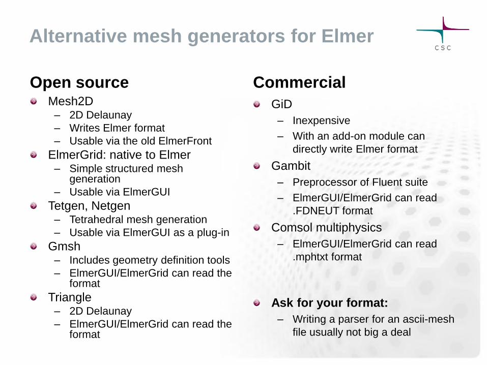
Alternative mesh generators for Elmer

Open source Mesh2D

– 2D Delaunay

– Writes Elmer format

– Usable via the old ElmerFront

ElmerGrid: native to Elmer – Simple structured mesh

generation

– Usable via ElmerGUI

Tetgen, Netgen – Tetrahedral mesh generation

– Usable via ElmerGUI as a plug-in

Gmsh – Includes geometry definition tools

– ElmerGUI/ElmerGrid can read the format

Triangle – 2D Delaunay

– ElmerGUI/ElmerGrid can read the format

Commercial

GiD

– Inexpensive

– With an add-on module can

directly write Elmer format

Gambit

– Preprocessor of Fluent suite

– ElmerGUI/ElmerGrid can read

.FDNEUT format

Comsol multiphysics

– ElmerGUI/ElmerGrid can read

.mphtxt format

Ask for your format:

– Writing a parser for an ascii-mesh

file usually not big a deal

Mesh Generation tools – Poll (May 2012)

Importing meshes with ElmerGrid

ElmerGrid has a number parsers for various formats

Each format has a ”magic number”

ElmerGUI decides the format just from the suffix, for a few formats The first parameter defines the input file format:

1) .grd : Elmergrid file format

2) .mesh.* : Elmer input format

3) .ep : Elmer output format

4) .ansys : Ansys input format

5) .inp : Abaqus input format by Ideas

6) .fil : Abaqus output format

7) .FDNEUT : Gambit (Fidap) neutral file

8) .unv : Universal mesh file format

9) .mphtxt : Comsol Multiphysics mesh format

10) .dat : Fieldview format

11) .node,.ele: Triangle 2D mesh format

12) .mesh : Medit mesh format

13) .msh : GID mesh format

14) .msh : Gmsh mesh format

15) .ep.i : Partitioned ElmerPost format

The second parameter defines the output file format:

1) .grd : ElmerGrid file format

2) .mesh.* : ElmerSolver format (also partitioned .part format)

3) .ep : ElmerPost format

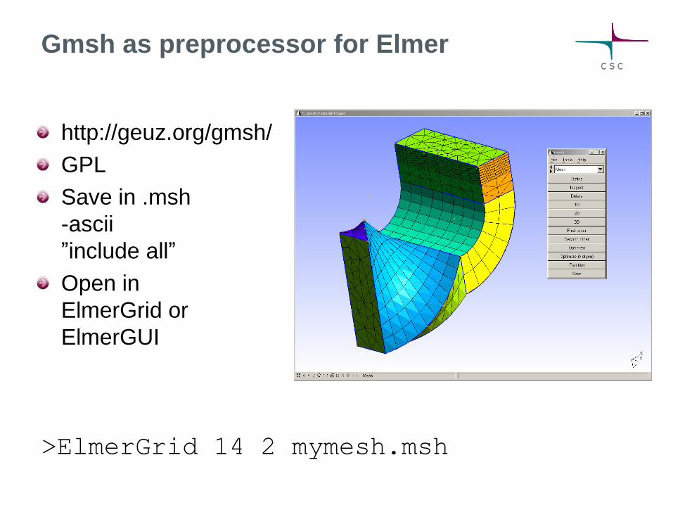
Gmsh as preprocessor for Elmer

http://geuz.org/gmsh/

GPL

Save in .msh

-ascii

”include all”

Open in

ElmerGrid or

ElmerGUI

>ElmerGrid 14 2 mymesh.msh

GiD as preprocessor to Elmer

Rather inexpensive

One month free!

Install export package

Use problemtype Elmer

Saves Elmer meshes

directly

Open source Commercial

Matlab, Excel, …

– Use SaveData to save results in

ascii matrix format

– Line plotting

Alternative postprocessors for Elmer

ElmerPost

– Postprocessor of Elmer suite

ParaView, Visit

– Use ResultOutputSolve to write

.vtu or .vtk

– Visualization of parallel data

OpenDX

– Supports some basic

elementtypes

Gmsh

– Use ResultOutputSolve to write

data

Gnuplot, R, Octave, …

– Use SaveData to save results in

ascii matrix format

– Line plotting

Visualization tools – Poll (May 2012)

Exporting 2D/3D data: ResultOutputSolve

Apart from saving the results in .ep format it is possble to use other

postrprocessing tools

ResultOutputSolve offers several formats

– vtk: Visualization tookit legacy format

– vtu: Visualization tookit XML format

– Gid: GiD software from CIMNE: http://gid.cimne.upc.es

– Gmsh: Gmsh software: http://www.geuz.org/gmsh

– Dx: OpenDx software

Vtu is the recommended format!

– offers parallel data handling capabilities

– Has binary and single precision formats for saving disk space

Exporting 2D/3D data: ResultOutputSolve

An example shows how to save data in unstructured XML VTK (.vtu) files to

directory ”results” in single precision binary format.

Solver n

Exec Solver = after timestep

Equation = "result output"

Procedure = "ResultOutputSolve" "ResultOutputSolver"

Output File Name = "case"

Output Format = String ”vtu”

Binary Output = True

Single Precision = True

End

Derived fields

Many solvers have internal options for computing derived fields (fluxes, heating powers,…)

Elmer offers several auxiliary solvers

– SaveMaterials: makes a material parameter into field variable

– Streamlines: computes the streamlines of 2D flow

– FluxComputation: given potential, computes the flux q = - c

– VorticitySolver: computes the vorticity of flow, w =

– PotentialSolver: given flux, compute the potential - c = q

– Filtered Data: compute filtered data from time series (mean, fourier coefficients,…)

– …

Usually auxiliary data need to be computed only after the iterative solution is ready

– Exec Solver = after timestep

– Exec Solver = after all

– Exec Solver = before saving

Derived lower dimensional data

Derived boundary data

– SaveLine: Computes fluxes on-the-fly

Derived lumped (or 0D) data

– SaveScalars: Computes a large number of different quantities

on-the-fly

– FluidicForce: compute the fluidic force acting on a surface

– ElectricForce: compute the electrostatic froce using the Maxwell

stress tensor

– Many solvers compute lumped quantities internally for later use

(Capacitance, Lumped spring,…)

Saving 1D data: SaveLine

Lines of interest may be defined on-the-fly

Flux computation using integration points on the

boundary – not the most accurate

By default saves all existing field variables

Saving 1D data: SaveLine…

Solver n

Equation = "SaveLine"

Procedure = File "SaveData" "SaveLine"

Filename = "g.dat"

File Append = Logical True

Polyline Coordinates(2,2) = Real 0.25 -1 0.25 2.0

End

Boundary Condition m

Save Line = Logical True

End

Saving 0D data: SaveScalars

Operators on bodies

Statistical operators

– Min, max, min abs, max abs, mean, variance, deviation

Integral operators (quadratures on bodies)

– volume, int mean, int variance

– Diffusive energy, convective energy, potential energy

Operators on boundaries

Statistical operators

– Boundary min, boundary max, boundary min abs, max abs, mean, boundary variance, boundary deviation, boundary sum

– Min, max, minabs, maxabs, mean

Integral operators (quadratures on boundary)

– area

– Diffusive flux, convective flux

Other operators

– nonlinear change, steady state change, time, timestep size,…

Saving 0D data: SaveScalars…

Solver n

Exec Solver = after timestep

Equation = String SaveScalars

Procedure = File "SaveData" "SaveScalars"

Filename = File "f.dat"

Variable 1 = String Temperature

Operator 1 = String max

Variable 2 = String Temperature

Operator 2 = String min

Variable 3 = String Temperature

Operator 3 = String mean

End

Boundary Condition m

Save Scalars = Logical True

End

Case: TwelveSolvers

Natural convection with ten auxialiary

solvers

Case: Motivation

The purpose of the example is to show the flexibility

of the modular structure

The users should not be afraid to add new atomistic

solvers to perform specific tasks

A case of 12 solvers is rather rare, yet not totally

unrealitistic

Case: preliminaries

Square with hot

wall on right and

cold wall on left

Filled with viscous

fluid

Bouyancy modeled

with Boussinesq

approximation

Temperature

difference initiates

a convection roll

COLD HOT

Case: 12 solvers

1. Heat Equation

2. Navier-Stokes

1. FluxSolver: solve the heat flux

2. StreamSolver

3. VorticitySolver

4. DivergenceSolver

5. ShearrateSolver

6. IsosurfaceSolver

7. ResultOutputSolver

8. SaveGridData

9. SaveLine

10.SaveScalars

Case: Computational mesh

10000 bilinear

elements

Case: Navier-Stokes, Primary fields

Pressure Velocity

Case: Heat equation, primary field

Case: Derived field, vorticity

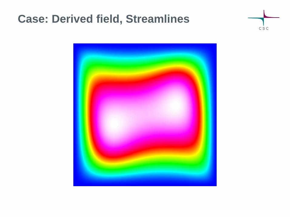
Case: Derived field, Streamlines

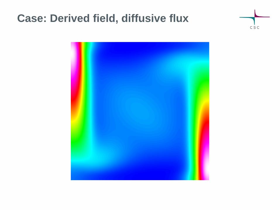
Case: Derived field, diffusive flux

Case: Derived field, Shearrate

Example:

view in GiD

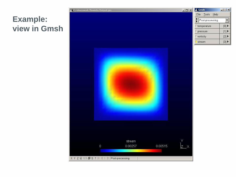
Example:

view in Gmsh

Case: View in Paraview

Conclusions

Preprocessors

– Simple structured: ElmerGrid

– Unstructured: Gmsh or netgen

– Complex: GiD or Salome

Postprocessors

– Basic use: ElmerPost

– Advanced use: Paraview