emergent 1d ising behavior in an elementary...

January 21, 2009 17:37 WSPC/141-IJMPC 01351

International Journal of Modern Physics CVol. 20, No. 1 (2009) 133–145c© World Scientific Publishing Company

EMERGENT 1D ISING BEHAVIOR IN AN ELEMENTARY

CELLULAR AUTOMATON MODEL

PAUL G. KASSEBAUM∗ and GERMANO S. IANNACCHIONE†

Physics Department, Worcester Polytechnic Instiute

100 Institute Road, Worcester, Massachusetts 01609, United States∗[email protected]

†[email protected]

Received 7 June 2008Accepted 11 July 2008

The fundamental nature of an evolving one-dimensional (1D) Ising model is investigatedwith an elementary cellular automaton (CA) simulation. The emergent CA simulationemploys an ensemble of cells in one spatial dimension, each cell capable of two mi-crostates interacting with simple nearest-neighbor rules and incorporating an externalfield. The behavior of the CA model provides insight into the dynamics of coupledtwo-state systems not expressible by exact analytical solutions. For instance, state pro-gression graphs show the causal dynamics of a system through time in relation to thesystem’s entropy. Unique graphical analysis techniques are introduced through differencepatterns, diffusion patterns, and state progression graphs of the 1D ensemble visualizingthe evolution. All analyses are consistent with the known behavior of the 1D Ising sys-tem. The CA simulation and new pattern recognition techniques are scalable (in bothdimension, complexity, and size) and have many potential applications such as complexdesign of materials, control of agent systems, and evolutionary mechanism design.

Keywords: Ising; cellular automata; automaton.

PACS Nos.: 11.25.Hf, 123.1K.

1. Introduction

Fundamentally, the Ising model consists of an ensemble of members that can exist

in one of two possible states (e.g., up or down). The state of a particular member

depends upon the states of other members of the ensemble (nearest, next-nearest

neighbors, etc. or averaged overall members) as well as its coupling to an external

field that is conjugate to the microstate. Advantages of this model are the clarity

of its construction, even in multiple dimensions, and its wide range of applicability

such as magnetic spins (the original system considered by Ising), financial markets,

robotic control, chemical reactions, etc., to name a few.

However, there are a number of difficulties with an Ising approach,1 namely,

there is no systematic formulation for determining the Ising partition function.

133


134 P. G. Kassebaum & G. S. Iannacchione

Despite the conceptual simplicity of the Ising approach, analytic solutions exist only

in one dimension and in two dimensions without an external field. These difficulties

warrant the continued and active efforts in applying and studying the Ising model.

A relatively new approach, sometimes referred to as “emergent theory,” has as

its fundamental principle that simple rules of interaction between members of an

ensemble can lead to complex behavior. This method has simple rules of member

interaction stand in for complex analytical models and allows an evolution of cellular

ensembles to be easily monitored. This principle as it applies to an Ising system is

the primary focus of this work.

1.1. Historical review

The 2004 study by Jarkko Kari2 serves as an excellent tutorial in cellular automaton

(CA) theory. This survey begins with CA models for reproduction in 1962 by E. F.

Moore up to Stephen Wolfram’s seminal work in 2002.3,4 However, perhaps the most

influential foundational work on CA theory was published by John von Neumann.5

CAs were shown to be useful in simulating the Navier–Stokes equations in the

1986 study by Frisch.10 Entropy considerations of CAs were discussed in 1992 by

Hurd.11 Conservative CA systems were investigated in 2002 by Boccara.12

Textbooks written on physical investigations utilizing CAs include the 1998

work by Chopart13 and the 2002 work by Stephen Wolfram.4

To the best of our knowledge, the earliest application of CA to statistical me-

chanics was done in 1983 by Stephen Wolfram.6 While this work was a comprehen-

sive investigation of the topic, it only alluded to the Ising model. Several papers

were independently written in response to Wolfram’s by many authors.7–9

The approaches taken by these later works eschewed the principles described by

Wolfram, viz., to keep CA models as simple as possible and to allow the complexity

to emerge despite this simplicity. The CAs in later works were very complex upon

construction. Simpler CAs equivalent to the Ising model and their fundamental

nature have not been investigated.

1.2. Findings

We show that a 1D Ising system can be realized in the form of an elementary cel-

lular automaton. Several interesting symmetries of the Ising system were revealed

by the computational experiments performed in this work. Percolations through

the system, studied by the difference and diffusion patterns, are found to exhibit

complex, stochastic behavior. In addition, we introduce state progression graphs

of these finite computational systems that lend new interpretations of the evolu-

tion of entropy and raise new questions of their graph theoretical structure. These

graphs show the causal dynamics of a system through time in relation to the sys-

tem’s entropy and provide a unique tool in the computational study of interacting

systems.


Emergent 1D Ising Behavior in an Elementary CA Model 135

1.3. Map of the paper

In what follows, each emergent methodology for studying the Ising system will be

encapsulated in its own section. Each methodology is introduced in an overview

subsection, wherein a method is briefly elucidated in terms of its functioning and

meaning. The following subsection details a procedural construction of the method

for its reproduction. Each method’s section is concluded with a discussion of results

gathered through its use. The methods considered as a whole are discussed in the

concluding section of the paper.

2. An Elementary Cellular Automaton Model

2.1. Overview

The emergent model used in this work is expressed as a cellular automaton (CA).

The progression rules in Fig. 1 describe the evolution of a cell’s state influenced

solely by its nearest neighbors, and not by a global influence. Ambivalent cases are

reconciled by symmetry considerations. Essentially, if a member’s neighbors agree

in orientation, then the member will acquiesce.

The elementary CA model shown in Fig. 1 maps onto the 1D Ising model with

only nearest-neighbor interactions. The “J” coupling between states (spins) are not

adjusted here (equivalent to being fixed to unity).

An Ising system with a global influence can be constructed by altering the

progression rule described above. With a global influence, a member more easily

acquiesces to neighbors that are in agreement with it.

2.2. Procedure

The model employs a Mathematica platform to implement and study the elementary

cellular automata. The progression rules described graphically above may be defined

as mathematical functions. The value a(t, i) for a member at position i on time step

t can be defined as

a(t, i) = f{a(t− 1, i − 1), a(t − 1, i), a(t − 1, i + 1)} , (1)

where various progression rules correspond to different choices of the function f .

The CA model given in Fig. 1 corresponds to

f(x, y, 0) = 0 and f(x, y, 1) = 1 , (2)

Fig. 1. Representation of a cellular automaton rule set that is isomorphic to an Ising system inisolation. The three top cells represent the cell of interest and its nearest neighbors. Open (0) andfilled (1) cells denote one of the two possible states. The lone bottom cell shows the resulting stateof the cell of interest.



members

time steps

cyclic boundaryt = 0

Fig. 2. The emergent behavior of the CA in Fig. 1 given a disordered initial condition of 200 mem-bers long played out for 100 progressions. The spatial dimension runs left to right; the temporal,top to bottom. The spatial dimension has cyclical boundary conditions.

where x and y represent either the value 1 or 0. This progression of number sets

can be fully enumerated as

{0, 0, 0} → 0 , {0, 0, 1} → 1 , {0, 1, 0} → 0 , {0, 1, 1} → 1 ,

{1, 0, 0} → 0 , {1, 0, 1} → 1 , {1, 1, 0} → 0 , {1, 1, 1} → 1 .

The 1D cellular automata in this study have cyclical boundary conditions, where

the left-most cell is treated as being physically adjacent to the right-most cell.

2.3. Discussion

The emergent behavior of an Ising system at zero field, depicted in Fig. 2, exhibits

grain boundary behavior. Small grains progressively coalesce into larger grains.

While most of the members tend toward the homogeneity of alternating neighborly

states, certain grains are able to persist indefinitely. Throughout the time evolution

of states, the total number of black cells remains constant, as do the white. This

is an expected consequence of conservation considerations given that the system is

isolated.

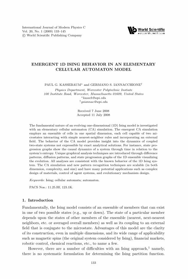
For scenarios involving a global influence, the CA progression rule-set in Fig. 1

is altered. Figure 3(a) depicts the weakest augmentation of a global influence. Grain

boundary behavior is again seen. Of course, the system eventually reaches a state

in accordance with the global influence. The time it takes for a system to reach

saturation of one state is studied later.

Figures 3(b) and 3(c) depict the expected evolution with progressively increasing

global (field). Note that each panel in Fig. 3 represents a unique, augmented rule-

set.

3. Difference Patterns

3.1. Overview

Difference patterns facilitate analysis of how a single bit of information percolates

through an Ising system. Given the emergent behavior of a system seeded by a



a)

(a)

b)

(b)

c)

(c)

Fig. 3. From (a) to (c) are progressively augmented CAs given a disordered initial condition200 members long. They are each cut off once they fully acquiesce to the external influence.

particular initial condition, the seeding may be altered by a single cell variation

and contrasted with the emergent behaviors of the two instances: hence, the term

“difference pattern”.

The transient characteristics of a CA can be readily studied using difference

patterns. As the transient behavior of information flow through a difference pattern

halts, so too does the global transient behavior of the CA.

3.2. Procedure

A difference pattern may be constructed as follows:

(i) seed a CA; record the seeding and its emergence;

(ii) alter the seeding accordingly; record a new emergence;

(iii) subtract the two emergences.

The transient period of a difference pattern may be discerned by the following

algorithm:

(i) construct a difference pattern of sufficient time length;

(ii) copy the difference pattern;

(iii) alter the copy by shifting each time instance by one spatial unit;

(iv) alter the original by removing its initial time instance;

(v) take the difference of the original and the copy;

(vi) measure the number of time steps that have a null value from the final time

instance backward;

(vii) subtract this number from the total time steps.

3.3. Discussion

Figure 4 depicts erratic percolations that fluctuate with regard to direction, speed,

and breadth. A difference pattern’s “speed” refers to the horizontal distance a



Fig. 4. Difference pattern of Ising system with no global influence. Each panel evolved from adifferent initial condition. Each evolution has been cut off where it begins to be predictable.

Fig. 5. Statistical analysis of the number of progressions required before a difference patternbecomes predictable (steady state) with no global influence and various members. All simulationswere performed for 1000 timesteps. The upper four probabilities ticked off are the maximum valuesfor each experiment. The lower four probabilities are the average values.

pattern travels in a single time step. Its “breadth” refers to the horizontal width at

a particular instant.

The erratic behavior of a percolation eventually extinguishes, giving way to

perpetual predictability. Figure 5 depicts a statistical analysis of the time it takes

for an isolated Ising system to reach a steady state. The probability is defined as the

number of evolutions that reached steady state at a particular time step normalized

by the total number of evolutions observed. At a time step equal to half the number

of members in the system, there is a time horizon beyond which the system will be

at a steady state with absolute certainty. The probability of reaching a steady state

spikes at a time near zero and a time near the horizon. The probability density

function appears to be of a stochastic nature.

Figure 6 repeats the analysis shown in Fig. 5 but on a system with a small

external field. Regardless of the number of members in the system, the probability



0.5 10.95.7 33

0.138

100 Members200 ``300 ``400 ``

Time steps

Probability

0.001

Fig. 6. Statistical analysis of the number of progressions required before the difference patternbecomes predictable with minimal global influence and various members. The statistical analysisof each system with a fixed number of members was performed over 1000 experiments. The averagetime to equilibrium and the standard deviation are shown on the abscissa. The extreme values ofthe data are shown on the ordinate.

density function (PDF) of the transient period decreases through what appears to

be an inflection point and then asymptotically approaches zero. The deviation of

the PDF around its expected value is not negligible close to time equal to zero.

4. Diffusion Patterns

4.1. Overview

Whereas a difference pattern is made by contrasting two instances differing by a

single change in initial conditions, diffusion patterns are made by numerous such

contrasts. The result is an intuitive visual representation of the statistical charac-

teristics of how information flows through a system.

4.2. Procedure

A diffusion pattern may be constructed by flipping one member of the initial con-

dition at a time and then combining the emergence of each case. This process may

be described algorithmically as follows:

(i) construct a seed; record the emergence;

(ii) copy the original seed and alter it by one bit; record its emergence;

(iii) alter the original seed by a different bit than the previous; record its emergence;

(iv) repeat until every bit has been treated;

(v) sum all of the emergences.



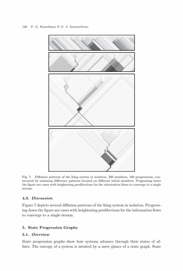
Fig. 7. Diffusion patterns of the Ising system in isolation, 200 members, 100 progressions, con-structed by summing difference patterns focused on different initial members. Progressing downthe figure are cases with heightening predilections for the information flows to converge to a singlestream.

4.3. Discussion

Figure 7 depicts several diffusion patterns of the Ising system in isolation. Progress-

ing down the figure are cases with heightening predilections for the information flows

to converge to a single stream.

5. State Progression Graphs

5.1. Overview

State progression graphs show how systems advance through their states of af-

fairs. The entropy of a system is intuited by a mere glance of a state graph. State



graphs may be constructed over a finite set of members, constituting a particular

system.

More interestingly, a finite set of members may be considered to constitute not

an actual system in reality, but rather a contiguous subset of a system isolated

artificially by an observer. Consequentially, a state graph made up of the union of

subsets represents the system independent of observation.

5.2. Procedure

State progression graphs are produced by applying a rule-set to a prescribed state

with a particular number of members and recording the resultant causal relation-

ship. After collecting all of the possible causal relationships for a system of a given

size, a graph like the one shown in Fig. 8 can be produced.

State graphs irrelevant to observation are made similarly, but require a mapping

of analogous states of affairs. For instance, a system of four members might take

on the state (0, 0, 0, 1). This state is equivalent to (0, 0, 1) in a system of three

members. Of course, the required mapping is only a statement of the equivalence

between binary numbers with arbitrarily many leading zeros.

5.3. Discussion

In the vernacular graph theory, a “community” is a connected subgraph.

Figure 8 depicts the state graph of the Ising system with eight members in isola-

tion, consisting of several communities. The simplest community is trivial, wherein

a state gives rise to itself. The next least trivial community has a periodic nature

shown in Fig. 8(d). A variation on the latter community has certain states that can

only be accessed as initial conditions, proceeded by periodicity shown in Figs. 8(b)

and 8(c). The most interesting community is displayed in Fig. 8(a).

Fig. 8. State progression graphs for an eight-member 1D Ising system in isolation. Each commu-nity is symmetric; so, only half of each is shown.



Fig. 9. Interesting communities of ten (top) and eight (bottom) member state progression graphsof the Ising system with no global influence.

Within the interesting community, the system tends toward periodicity between

two states that may be reached in numerous different ways. The community is

symmetric over reflection about the two fluctuating states. The final two states

over which it oscillates are symmetric over a shift by one spatial unit.

The less interesting communities result in a periodic progression over a number

of states equal to the number of members in the system or lesser factors of that

number. In the instance of Fig. 8, there are eight members in the system; so,

the majority of the communities result in periodicity over eight or four states.

Interesting communities only arise in systems with an even number of members.

Figure 9 depicts interesting communities of eight and ten members. Both are

symmetric over reflection about the two fluctuating states.

Figure 10 depicts interesting communities of an Ising system with eight members

and various levels of global influence.

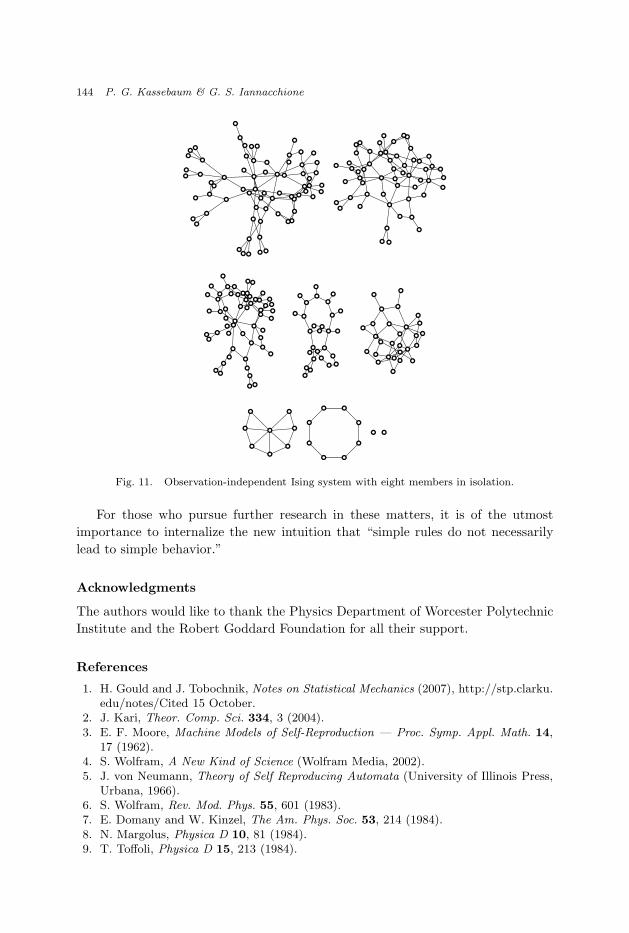
Figure 11 depicts the observation-independent state graph of an Ising system

with eight members in isolation. An “observation-independent” CA with rule-set r is

the union of N evolutions each with i members,⋃

N

iCA(r, i). Further investigations

into the nature of these graphs is necessary and will be pursued in a future work.

6. Conclusions

The 1D Ising system’s fundamental nature was partially unfurled with several new

interpretation tools. The scope of this investigation was to introduce these tools

and present a case for their merit. No analytical models, or discretizations thereof,

were used in the study. Nor were any artificial complexities imposed on the cellular

automata. Instead, cellular automata were studied in their own right as systems

equivalent to Ising systems.



Fig. 10. Interesting communities of eight member state progression graphs with increasing ex-ternal field from zero (top) to higher values (bottom). The highest global influence scenario is

omitted.

Despite the simplicity of the systems studied, each interpretation revealed un-

derlying complexity and interesting symmetries. More questions have been raised

by this investigation than were answered. What follows are suggestions for future

study:

• Rigorous characterization of the transient behavior of the 1D Ising system;

• Develop physical implications of diffusion patterns;

• Graph theoretical analysis of state progression graphs;

• Generalization of the cellular automata in terms of dimensionality and range of

neighborly influence.



Fig. 11. Observation-independent Ising system with eight members in isolation.

For those who pursue further research in these matters, it is of the utmost

importance to internalize the new intuition that “simple rules do not necessarily

lead to simple behavior.”

Acknowledgments

The authors would like to thank the Physics Department of Worcester Polytechnic

Institute and the Robert Goddard Foundation for all their support.

References

1. H. Gould and J. Tobochnik, Notes on Statistical Mechanics (2007), http://stp.clarku.edu/notes/Cited 15 October.

2. J. Kari, Theor. Comp. Sci. 334, 3 (2004).3. E. F. Moore, Machine Models of Self-Reproduction — Proc. Symp. Appl. Math. 14,

17 (1962).4. S. Wolfram, A New Kind of Science (Wolfram Media, 2002).5. J. von Neumann, Theory of Self Reproducing Automata (University of Illinois Press,

Urbana, 1966).6. S. Wolfram, Rev. Mod. Phys. 55, 601 (1983).7. E. Domany and W. Kinzel, The Am. Phys. Soc. 53, 214 (1984).8. N. Margolus, Physica D 10, 81 (1984).9. T. Toffoli, Physica D 15, 213 (1984).



10. U. Frisch, B. Hasslacher and Y. Pomeau, Phys. Rev. Lett. 56, 1505 (1986).11. L. P. Hurd, J. Kari and K. Culik, Ergodic Theor. Dyn. Syst. 12, 255 (1992).12. N. Boccara and H. Fuks, Fund. Inform. 52, 1 (2002).13. B. Chopart and M. Droz, Cellular Automata Modeling of Physical Systems (Cam-

bridge University Press, Cambridge, 1998).

emergent 1d ising behavior in an elementary...

Documents