.M414

WORKING PAPER

ALFRED P. SLOAN SCHOOL OF MANAGEMENT

EMERGING APPROACHES TO

RETAIL OUTLET MANAGEMENT

Gary L. LilienM.I.T.

Ambar G . RaoNew York University

WP 882-76 November 1976

MASSACHUSETTS

INSTITUTE OF TECHNOLOGY50 MEMORIAL DRIVE

CAMBRIDGE, MASSACHUSETTS 02139

EMERGING APPROACHES TO

RETAIL OUTLET MANAGEMENT

Gary L. LilienM.I.T.

Ambar G. RaoNew York University

WP 882-76 November 1976

M.!.T. L!B:?ARIES

APR 2 8 1977

RECEIVtLD

Abstract

Major problems faced by the multi-outlet retailer include those of

strategic planning, tactical decisions and operational control. The

strategic planning questions include: How many outlets should be built

in the next Y years? In what cities should they be built? When?

Tactical decisions concern the selection of a particular site: What is

the potential of a particular site? What are the characteristics that

lead to the success of a particular site? What will be the impact of an

outlet on neighboring outlets? Operational control procedures include

exception reporting, detection of new trends, planning and monitoring

of advertising and promotional expenditures.

This paper reviews emerging quantitative approaches to retail out-

let management and shows how a few key concepts can be and have been used

in a variety of product areas.

0731008

-1-

Introduction :

In many industries, products are offered to consumers through company

controlled retail outlets. Some examples are supermarket chains, gaso-

line, banks, and fast foods, where the outlets are supermarkets, service

stations, branch banks and franchised restaurants respectively. As in other

industries, the problems of retail outlet management can be classified

into three groups — strategic planning, tactical decisions and operational

control.

The strategic planning questions are:

- How many outlets should be built in the next Y years?

- In what cities (markets) should they be built?

- When?

The tactical decisions concern the selection of specific sites — i.e.

- What is the potential of a specific site?

- What is the impact of changes in the environment on site potential, e.g.

construction of a motel on gas station sales?

- What is the impact of an outlet on a neighboring outlet?

Operational control procedures include

- exception reporting

- detection of new trends

- planning and monitoring of advertising and promotional expenditures.

In the past much of the quantitative work has focused on tactical

problems, particularly on site evaluation (see Green and Appelbaum [5] for a briefreview)

.

Strategic issues have largely been handled in an informal way. Recently,

some researchers have recognized that site potential is related to the

-2-

product or company "image" (see Stanley and Sewall [17] but they do not

indicate how image can be changed in a way that increases potential.

The purpose of this paper is to describe some emerging quantitative

approaches to retail outlet management, and to show how a few key concepts

can be and have been successfully used in a variety of product areas. The

paper does not exhaustively review the literature in retail outlet manage-

ment, but rather, highlights the important ideas that underlie problems in

this area.

1.0 Strategic Planning

Conventional market share analysis suggests that, after a building plan

is implemented, market share will equal outlet share. If this were the case,

the planning decision rules would be simple: build where the next unit of

outlet (equal to market) share brings the highest profit (perhaps in Net

Present Value terms) , continue building until either budget is exhausted,

or additional share does not produce acceptable returns.

Life is rarely this simple as several authors have pointed out (see

Kotler [10], pp. 786-788). Several reasons have been suggested for why

market share does not seem to increase linearly with outlet share, including

inequalities in promotional and outlet-quality effectiveness among companies,

some vague economies-of-scale argument, etc. , but a simple explanation for

this behavior is still the subject of debate (see Lilien [12] for one analysis)

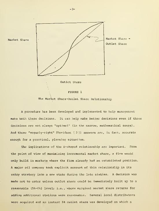
The important observation, however, is that a nonlinear, generally S-shaped

relationship exists between outlet share and market share, making the question

of how many outlets to build, and in what markets, considerably more complex

(Figure 1 illustrates this relationship)

.

-3-

Market Share

\

Outlet Share

FIGURE 1

Market Share

Outlet Share

The Market Share-Outlet Share Relationship

A procedure has been developed and implemented to help management

make both these decisions. It can help make better decisions even if those

decisions are not always "optimal" (in the narrow, mathematical sense)

.

And these "vaguely-right" (Davidson [ 3 ]) answers are, in fact, accurate

enough for a practical, planning situation.

The implications of the S-shaped relationship are important. From

the point of view of maximizing incremental market share, a firm would

only build in markets where the firm already had an established position.

A major oil company took explicit account of this relationship in its

entry strategy into a new state during the late sixties. A decision was

made not to enter unless outlet share could be immediately built up to a

reasonable (5%-6%) level; i.e., where marginal market share returns for

adding additional stations were reasonable. Several local distributors

were acquired and an instant 5% outlet share was developed on which a

-4-

building program was then based. Building up from scratch was recognized

as an unprofitable strategy. Thus when a company expands geographically,

the strategy should be to build up share quickly in each new market

before proceeding to the next. Simultaneous expansion into a large number

of new markets is likely to be unsuccessful, unless financial and managerial

constraints are non-existent.

Even after understanding this market share-outlet share relationship,

however, the development of plans are not straightforward.

1. 1 Using the S-Curve as Part of a Planning System

Suppose that a firm has empirically developed an S-curve for its

markets and now wants to know how many outlets to build in each of a large

number of markets during a several (say, five) year planning period.

Generally the first year results become budget items — building funds

are allocated in accordance with plan "year 1". The following year

results are used to prepare profit plan projections and to help allocate

outlet-site procurement funds (in anticipation of building)

.

Observe the nature of the managerial decision process: all planned

outlets may not always be built due to changing local building

codes, construction difficulties, lack of sites, etc. If an extra, "choice"

site becomes available in a desirable area, an outlet may be constructed

on it immediately, even if no money was originally allocated. What

management needs to know is whether to build five outlets or twenty outlets

in a given area. The different between (say) five and six outlets is

unimportant as it often washes out during implementation.

-5-

Before looking for a good, or "best" plan, let us examine how to

determine the value of a particular, known, plan. XYZ Company's plan for

market A may be to build three outlets this year and two in each of the

rest of the years of the planning horizon. Let us assume that the firm

has a forecast of competitive activity (building plans for all firms other

than XYZ) as well as market volume and volume growth rate, current and

forecast prices and margins, cost of land, etc. Thus XYZ has available

all the information needed to make an objective financial evaluation of

this situation as follows:

Step 1 : For each year of the planning period calculate XYZ's plans\

and industry plans. \

Step 2 : Use the S-curve relationship to find the outlet share and

thus the associated market share (MS ) for each year t.

Step 3: Multiply MS by the projected volume in the market to get

XYZ's volume, (Vol )

.

Step 4 : Multiply Vol by the projected gross margin (Mar ) to get

Gross Revenue (GRev )

.

Step 5

;

Adjust Gross Revenue by investment, debit factors to get

a cash flow associated with each year: CF .

Final Step : Determine the net present value (NPV) associated with the

plan as:

T CFNPV = I

^-—t=l (1-R)

where T is the planning horizon and R is the discount rate.

Now, if every outlet, (in NPV terms) were worth less than the one

built before it, the best building plan would be the one which first built

-6-

the outlet with the highest current incremental NPV, then the one with the

next highest, etc. But as the S-curve indicates, there are often increasing

returns in a building plan which must be considered. The procedure developed

takes this region of increasing returns into consideration. It is perhaps

best explained by an example.

Using the procedure on the preceeding page, we can calculate the NPV

associated with any building plan. Suppose XYZ has two markets to consider.

Market A and Market B, and has calculated the NPV associated with each

building plan in each market. Figure 2 displays the results:

NPV

1 2// of outlets

Market A

NPV 25

Total Building Constraint

-7-

PLAN

A B

TOTAL

NPV

15

30

45

55

TABLE 1 ; Example; Allocation Procedure Results

Note that here, if an incremental analysis were used (for Total Building

Constraint = 2) outlet number 2 would be built in Market B. This would yield

a total NPV of 25 instead of the best case, 30.

The procedure above looks not only at the value of single outlets but

of groups of outlets to assess their profitability. The actual mechanics

of the procedure, especially with building plans over time, are somewhat

technical and are treated elsewhere (see Lilien and Rao [11]). The important

point is that in practice the procedure has proved efficient, and easy to

use, producing results that are optimal or close to optimal. The procedure

was run on a 170-market, five-year planning problem considering 3,000 outlets.

The allocation procedure took less than a minute on an IBM 360-75; including

input-output and NPV calculations the entire procedure ran in well under

five minutes. This efficiency is important for allowing update runs and

sensitivity analyses at low cost.

This system has been used as an aid in outlet building planning at a

major U.S. Corporation since 1969. The procedure was used in the following

way:

-8-

(1) To generate allocation plans, given a set of assumptions and

inputs;

(2) To test the allocation against changes in those assumptions.

Step 2 is critical in implementation and use. Suppose the model-

allocation doesn't change with projected possible variation in land costs

but is very sensitive to variations in profit margin projections. Then

have your analysts spend most or all of their time firming up the margin

projection and forget about the land cost figures.

(3) To aid in determining the overall building allocation.

Outlets are an investment and firms have alternative uses for their

building capital. Then as many outlets should be built as still return

a positive NPV when discounted at the firm's cut-off or internal rate of

return. Thus, no overall building constraint is needed — rather, the

procedure should shut off when the incremental NPV for the last outlet

planned becomes zero or negative. The discount factor is another important

impact on the over-all building level as well as the allocation.

The model did not replace or transcend the manager; rather it helped

provide more meaningful inputs and thus more useful outputs. The managers

are involved at each step of shaping the final results and by being able

to control the process they grow to trust it. Managers learn a great deal

about their own decision situation and how it interacts with the firm's

problems. They become more secure in their own judgments as well.

To simmarize, the key idea here is that development of efficient

building plans requires explicit recognition of the S-curve relationship,

i.e. the impact of the new building upon the entire structure of the mar-

ket. Use of this relationship leads to significant improvements in retail

outlet building policies.

-9-

2.0 Site Selection and Site Potential

A second key problem faced by the multi-outlet retailer is, given the

decision to locate in a market area or city, where the outlet should be

placed. Approaches vary. Applebaum [2] reports that 10% of a sample of

170 large retail chains did no systematic analysis for location of retail

outlets. That same study had research expenditures varying widely, with

the average research per new location being about 1% of the site-investment

cost.

When Eastern Shopping Centers appraises a site, that location is"sub-

jected to a searching analysis covering current populations . . . population

trends, current and per capita income of the area, competing centers or re-

tailers, ... road patterns," etc. In contrast, a drug chain appraises a site

"just by taking a ride around a particular area, talking to some of the people

living there and getting a feel for the site's expansion capabilities."

(Duncan and Phillips [4]).

What seems called for is a structure for analyzing outlet site potential.

A variety of different models have been suggested to aid in the evaluation

and measurement of this potential, several of which are reviewed below.

These models share a common underlying structure, modified or customized

for the particular business or purchase situation. This structure can be

summarized as

(1) Site Potential = Local Sales Component

+

Transient Sales Component

Relationship (1) says that the sales potential at a particular site

has two separate components: those sales derived from people who live

-10-

nearby and those sales from people who are driving through, but who do not

live in the area. The nature and importance of these two components vary

considerably from product class to product class, but the basic structure

serves as a starting point for model development.

The transient component of sales is of great importance in product

classes such as gasoline and fast foods where a great deal of brand-to-brand

substitution is possible and where the purchase trip is often a secondary

part of another journey. We review models used in several different product

areas below.

2.1 Case 1: Gas Station Models

Reinitz [16] describes a model developed to estimate site potential

for gasoline. (The authors participated in several stages of the develop-

ment of this model) . In this model, the structure of which is appropriate

for the fast food business as well,

Site potential = f + f

where f = local area potential and

f = transient sales potential

The procedure used to estimate f and f is as follows:

i) Choose a local area radius, usually 1 mile. (Model results are

generally not sensitive to the size of this radius as long as it is

not too small) . Obtain the car population, gasoline usage and other

information descriptiveof the area.

ii) Obtain a census of, and ratings of, existing outlets along a number

of predetermined attributes: Let

r. . = rating of outlet i, in the trading area

along attribute j . j may be ease of

accessability , e.g.

-11-

iii) Obtain importance weights of these attributes from consumers

w. = average importance weight of attrubute j.

One key attribute to include is brand-image or market presence, linking this

model with the S-curve model in the previous section.

iv) Now estimate

(2 )

/ w.r .

.

^ 1 IDnew outlety w.r .

.

all outletsin tradingarea

X Area GasolinePotential

Fraction ofSales boughtlocally.

The other component, f , is calculated similarly, with a "road-leg"

replacing the local trading area, and traffic count data replacing "Area

Gasoline Potential".

The development for fast foods is essentially equivalent, with con-

sumption habit data replacing gasoline usage. Functional forms other than

{ 2 ) have been used as well, with no significant improvement in predictive

power.

2 -2 Case 2: Supermarket Site Potential

Much has been written on the art and science of supermarket site poten-

tial. Green and Applebaum[ 5 ] review the relevant literature. We highlight

here some important model-developments.

Applebaum [ 1 ] describes a procedure called an "analogue" approach,

based on the assumption that the drawing power of a site will be close to

that of other stores of the chain under similar conditions. A major diff-

culty is the identification of "similar" conditions.

Huff ([ 8 ] and [ 9 ]) eliminates this problem by using the following model:

-12-

P. .=

X X

S. ^T..^

J hi.

k=l'^ ^

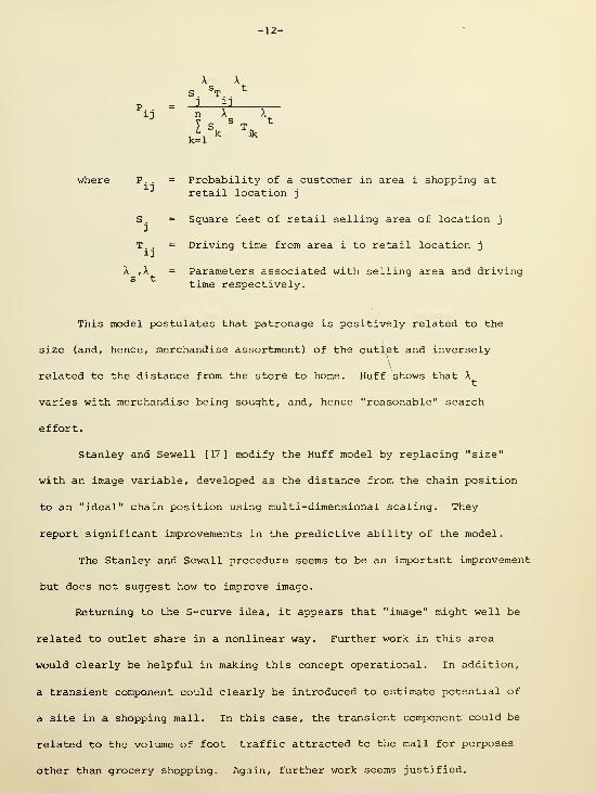
where P. . = Probability of a customer in area i shopping atij

retail location j

S. = Square feet of retail selling area of location j

T. . = Driving time from area i to retail location j

A ,X = Parameters associated with selling area and drivingtime respectively.

This model postulates that patronage is positively related to the

size (and, hence, merchandise assortment) of the outlet and inversely

related to the distance from the store to home. Huff shows that X

varies with merchandise being sought, and, hence "reasonable" search

effort.

Stanley and Sewell [17 ] modify the Huff model by replacing "size"

with an image variable, developed as the distance from the chain position

to an "ideal" chain position using multi-dimensional scaling. They

report significant improvements in the predictive ability of the model.

The Stanley and Sewall procedure seems to be an important improvement

but does not suggest how to improve image.

Returning to the S-curve idea, it appears that "image" might well be

related to outlet share in a nonlinear way. Further work in this area

would clearly be helpful in making this concept operational. In addition,

a transient component could clearly be introduced to estimate potential of

a site in a shopping mall. In this case, the transient component could be

related to the volume of foot traffic attracted to the mall for purposes

other than grocery shopping. Again, further work seems justified.

-13-

2. 3 Case 3; Automobile Dealerships

Hlavac and Little [6] describe a procedure for estimating site poten-

tial for automobile dealerships. The structure of the model is as follows:

Hlavac and Little assume that consumer selection of a dealer is related to

dealer location and customer preference for a particular auto-make, and is

relative to the attraction of all other dealers.

Consider one particular dealer, and split the region into a set of

areas, i = 1, ... I. Then define

g. = pull of the dealer on a buyer in geographic segment or area i;

h. = intrinsic pull of a dealer, independent of make (related

primarily to ease of accessability)

;

q. = make preference for the brand for buyers in segment i.

Then the pull of the dealer for buyers in geographic segment i is defined as

g. = h. * q.

and letting p. = the purchase probability for a buyer in area i then

g.

p. = V—^— (where j refers to the dealer, o to the dealer of interest)^ I ^ijJ

_ Pull of dealer x make preference

^ Pull of dealer x make preferenceall

dealers

The authors postulate an exponential drop off in dealer pull with distance

and equate make preference with brand share. A procedure is developed to

estimate the parameters of the dealer pull function and the model is shown

to fit data quite well.

-14-

This model, similar in spirit to the supermarket models, suggests a

brcind-size effect, included in the model as make-preference. And the

approach seems fruitful as the model fits data well. A limitation seems to

be the use of distance from dealership as a surrogate for convenience. And,

again, a S-curve effect might be incorporated with some benefit.

2.4 Case 4; Retail Banking

The authors have used a model similar to those above, for retail bank

outlet potential, where site-potential is modeled as

. , Site DrawSite potential = ^ Competing local site draws

Two phenomena are of interest here. The first is that a market share-

outlet share, S-type relationship exists in this market if we define market

share as share of new business.

The second phenomena is that site sales grow to long run potential faster

in areas with high property turnover. We see a relationship such as that

illustrated in Figure 3. Here area A has higher turnover and an outlet

there grows to its long term potential faster than one built in area B.

Similarly, account turnover in area A will continue to be higher than turn-

over in B throughout the life of the outlet. Management must then balance

the benefits of faster growth to potential with the continuing costs of long-

term account turnover in making site selection decisions for retail banks.

It is interesting to note the trend among local area retail banks

toward merger and adoption of a common name. Originally adopted for data-

processing economies, this move has resulted in additional benefits through

S-curve type share effects.

-15-

% ofpotential

A = high turnover area

/^ B = low turnover area

FIGURE 3:

Branch Bank Growth to Site Potential

-16-

There are many multi-outlet retailing industries not touched here

including giant retailers, hotels, and specialty item chains but the results

described are representative of the current state of knowledge and are indica-

tive of what is being used. The main point of the review in this section

is to suggest that structuring the site evaluation problem as Potential =

local + transient sales seems well adapted to problems in the retail outlet

industry, and should be exploited.

A key opportunity in this area is the integration of S-curve effects

into site evaluation. The results from the previous section suggest the

power of evaluating the total market impact of a building plan. That total

impact will not be the sum of the effect of individual sites, by themselves,

due to S-curve synergy. Thus, there is a major opportunity to improve these

models by including this synergistic effect of current market position in

evaluating building and divestment plans. Then a total market impact would

be estimated and the effect on market profitability more accurately gauged.

-17-

3 . Operat ional Control

Most multi-outlet retailers and, in fact, most commercial organizations

have sales and profit reporting systems. These systems report on various

measures of performance such as sales, cost, profits, etc. and compare what

happened in the current period with past performance. Such a comparison

implicitly assumes that this period should be like the last period or should

show some amount of growth — generally naive and uninformative assunptions.

To be meaningful and actionable, however, such comparisons must be

made to what should have happened. In order to say what should have happened

a model is required, linking control procedures to specific, quantitative

predictions of what performance should be or is expected to be like.

Modeling approaches to strategic planning and site location evaluation

have been described in the previous sections of this paper. An operational

control procedure can be built around these models. Consider a market area

in which a site expansion plan has been implemented. Using the model,

predictions of sales either in total or by product type in each period can

be developed. Thes e predictions necessarily use planned values for company

activities and estimates of competitive activity in the market. The predic-

tions can be displayed in tabular form (Figure 4) and in graphical form

(Figure 5; . The solid line in Figure 5 shows the historical sales in the

market, the dotted line the model forecasts.

In addition to the predictions, an estimate of forecast error is also

developed. This estimate can either be obtained directly from the model or

observed from the performance of the model against actual sales in the past.

Now suppose a specific marketing plan is implemented. Actual sales

for a period are reported, as are the actual values of company and competi-

tive activities. Actual sales are compared to sales predicted by the model.

\

Si

_-X

X"!^

_--X

f-t

-20-

If the difference between actual and predicted exceeds the previously determined

forecast error-limit, an exception report is issued. This report triggers

a "cause analysis" to determine why the exception occurred. (This is often

referred to as a "marketing audit".)

There are several possible circumstances that could have led to an

exception:

(a) company and competitive activities differed from assuirptions

used in the development of predictions. Management can investigate the

reasons for such differences, and develop administrative procedures to

ensure greater conformity to plans.

(b) a new type of activity (either company or competitive) not con-

sidered in the model structured occurred in the market. For example, a

novel type of promotion may have been introduced. In such cases, the model

needs to be enriched by including a factor representing the new activity.

(c) actual activities were in line with planned and estimated activities.

In such cases the model itself might be at fault. It needs to be re-examined.

In this case, the control procedure reports on itself and suggests that it be

improved.

Figure 6 shows some important types of exceptions that can occur. The

shaded area around the forecast indicates the range of variability to be

expected. As forecasts of periods further away in time are made, this range

increases. Exceptions 4, 5, and 6 in the figure are of particular interest. _

Exception 4 shows a situation where an increase in sales in one period .

Unsuccessful promotions often present such sales profiles. Exceptions 5 and

6 are early indicators of developing trends.

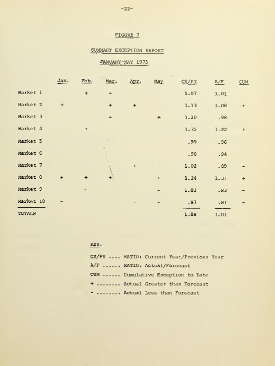
Figure 7 shows a convenient way to display the exception information,

and relate period sales, and cumulative sales to date, to predictions.

FIGURE 6

UPDATE STATUS — TREND ANALYSIS

DATA BEHAVIOR: STATUS REPORT

4.

IN CONTROL

UPDATE EXCEPTION

LAST POINT EXCEPTION,RETURN TO NORMAL TREND

UPDATE AND LAST POINTBOTH EXCEPTIONS

UPDATE AND LAST POINTBOTH EXCEPTIONS,POSSIBLE NEW TREND

CUMULATIVE EXCEPTIONNEW TREND

-22-

FIGURE 7

SUMMARY EXCEPTION REPORT

JANUARY-MAY 1975

Market 1

Market 2

Market 3

Market 4

Market 5

Market 6

Market 7

Market 8

Market 9

Market 10

TOTALS

Jan . Feb . Mar . Apr . May

+

+ + +

+

+

CY/PY

-23-

Systems such as that outlined above have been implemented by the authors

in several organizations. Yorke [18] gives details of one system that has

proven to be managerially useful. Rao and Shapiro [13] develop some new,

sophisticated forecasting methods that have proven to be useful in several

forecasting systems. Rao and Lilien [14] show how the effects of promotion

can be incorporated in a forecasting system to improve forecasting accuracy

and to better assess the relative impact of promotional programs. Rao and

Miller [15] describe some powerful methods of assessing the impact of product

advertising on sales and indicate how these methods, too, can be incorporated

into a forecasting and control system.

These developments are indicative of the state of the art. Systems

and procedures are currently available for operational reporting and control

of retail outlet performance which intelligently integrate models and data

into managerially useful information. They invariably reduce the volume of

reports, highlight important information, and indicate potential problems

and opportunities in a timely, yet routine fashion. They integrate model

building research into day to day operational control, and specify the

parameters of a useful, usable management information system, and associated

data base.

-

-24-

4.0 Conclusions

Our aim in this paper has been selective rather than exhaustive. We

point out that quantitative approaches to problems of retail outlet manage-

ment are emerging which are of use in problems of strategic and tactical

planning as well as operational control. Underlying these approaches are

a few key ideas:

1. Outlet share is generally related to share of market in a nonlinear

way. This relationship bears important impact on the development

of strategic building plans as well as in the evaluation of retail

site operations.

2. Structuring the problem of evaluating site potential as

potential = local component + transient component

has been quite successful and should be exploited.

3. The heart of a good operational control procedure is a set of

accurate forecasting models linked to exception reporting capa-

bilities. Successful models have been developed which can great-

ly inprove the operation of many such systems.

There is much need for new research in this field. However, there is

much more need for integration and implementation of existing methodology.

Many new tools and concepts are now available; the challenge to the multi-

outlet retailer is to make use of them.

-25-

REFERENCES

1. ApplebaiJin, William. "Methods for Determining Store Trade Areas,Market Penetrations and Potential Sales," Journal of MarketingResearch , Volume 3 (May 1966)

.

2. Applebaum, William. "Survey of Store Location by Retail Chains,"in Guide to Store Location Research , Curt Kornblau (ed) (Reading,MA: Addison-Wesley, 1968) .

3. Davidson, Sidney, "As I See It," Forbes (April 1, 1970).

4. Duncan, Delbert J. and Charles F. Phillips. Retailing; Principlescind Methods (Homewood, IL: Richard D. Irwin, 1967) .

5. Green, Howard L. and William Applebaum. "The Status of ComputerApplications to Store Location Research," paper presented at the 71stAnnual Meeting of the Association of American Geographers, MilwaukeeWisconsin (April 23, 1975).

6. Hlavac, Theodore E. Jr., and John D. C. little. "A Geographic Modelof an Urban Automobile Market," in Applications of Management Sciencein Marketing , Montgomery and Urban (ed.) (Englewood Cliffs: Prentice-Hall, 1970) .

7. Huff, David L. Determination of Inter-Urban Retail Trade Areas(Los Angeles: University of California, Real Estate Research Program,

1962).

8. Huff, David L. "A Probabilistic Analysis of Consumer Spatial Behavior,"in Emerging Concepts in Marketing, William S. Decker, (ed.) (Chicago:Americcin Marketing Association, 1963) .

9. Huff, David L. "Defining and Estimating a Trade Area," Journal of

Marketing, Vol. 28 (July 1964)

.

10. Kotler, Philip. Marketing Management: Analysis, Planning and Control ,

2nd edition (Englewood Cliffs: Prentice Hall, 1972).

11. Lilien, Gary L. and Ambar G. Rao. "A Model for Allocating RetailOutlet Building Resources Across Market Areas," Operations Research ,

Volume 24, Number 1 (January-February 1976)

.

12. Lilien, Gary L. "A Market Share-Outlet Share Model," Working draft,

September 1976.

13. Rao, Ambar G. and Arthur Shapiro, "Adaptive Smoothing Using Evolutionary

Spectra," Management Science, Volume 17, Number 3 (November 1970).

-26-

14. Rao, Ambar G. and Gary L. Lilian. "A System of Promotional Models,"Management Science , Volume 19, Number 2 (October 1972)

.

15. Rao, Ambar G. and Peter B. Miller. "Advertising/Sales Response Func-tions," Journal of Advertising Research , Volume 15, Number 2 (April

1975) .

16. Reinitz, Rudolph C. "A Sales Forecasting Model for Gasoline ServiceStations," private correspondence.

17. Stanley, Thomas J. and Murphy A. Sewall. "Image Inputs to a Proba-bilistic Model: Predicting Retail Potential," Journal of Marketing ,

Volume 40, Number 3 (July 1976).

18. Yorke, Carol E. "A Sales Planning and Analysis System," IEEE EngineeringManagement Review , Volume 2, Number 3 (September 1974)

.