emmemmmmmmenie periods required to … · optimized observation periods required to achieve...
TRANSCRIPT

'0,193 644 OPTIMIZED OBSERVATION PERIODS REQUIRED TO ACHIEVE 1/1 1'GEODETIC ACCURACIES USING THE GLOBAL POSITIONING SYSTEM(U) NAVAL POSTGRADUATE SCHOOL MONTEREY CA R H BOUCHARD
IUNCLASSIFIED MR 88 F/G 17/?EmmEmmmmmmEniEEEEnnEmhEEmhhElllllEllllllEEEIIEIIIEEEEIIEmhEIIIIEIIIIIIEIEEE".I

C323
1111 = L 1 1.216L
11111 1.11.-8111112 1 -. 11.6
MICROCOPY R(SOLUT"O list CHART
L FILE COP
4 NAVAL POSTGRADUATE SCHOOLm Monterey, California
spSTA %~ 00'0
~THESIS
OPTIMIZED OBSERVATION PERIODSREQUIRED TO ACHIEVE GEODETIC ACCURACIES
USING TIlE GLOBAL POSITIONING SYSTEM
by
Richard I. Bouchard
March 1988
Co-Advisor Stevens 11. TuckerCo-Advisor Narendra K. Saxena
Approved for public release; distribution is unlimited.
a,!

RLPOR r DOCUNIFNI .. lON I'M,1
n V 'r ~~~~3 Distib-u: n A~ail,'! ot R ,!,-
L1-:.2 ,*: *..t Appro-.Ckd t'r pkun!ic rcas': distribution is uniun~lJ.
-a - P~- i C .0 . Oi...e S. , nii o!. tn- r; r.
\~~~~~'~~~1 \a~'~iuae~ho ' ., . 5~al Pl\ ±dua(iL School
Mi-r CA. 'o'.43. 'ii' \iterc\. ('A~4. i"ta I::' Sr r . S . a! i O a .. r. 'o 01r . S. m Iro Prc_ ,n.L I r rurrrI Icnt N.I.n:,on
Pr'r x 11 Lemer-te\t P--- ~ " ~~' ~kI t-
.1 .: .- 2.: ,-'.'.. .1".' IlNl\1Z[D OBISERVATION P[RIODS REQUIRED) 10 ACHIEVE (iLODLTIC.*\C~~.ChS I S\( [IEGLOBAL. POSITIONING SYSTEMN
a.A..-iRichard I1. Bouchard;.wa I ve R pb-' I t C,%ertd i-4 Da', ot R!roit oeir ,p'ii jjy, I i Pace Count
\Ia'ter Ihi F.M nI)karch PAS 1 74
:S s. t!nntr \nt;,: j' [he iesexpres~sed in this thesis are those of the author and do not r taect the official policy, or po-Nltiofl of thle lDepuiment of Defense or the U.S. Government.
* - (',w: C &'s 13 Sut';ect Terms ; (011irlde 011 fe~e"te qj neeuetar.% and Jelfwf bt 6'd.- k ,Umferi
* F .~- Global Positioning System, relative geodesy. Trimible 4'JLIOSX, long baseline decteirmination.% ~triple difference, GPS, P'DOP. optimized observing periods. geodetic accuracy.
S It~a't I , m:i ,'*O e . L r #I,,, e;rY anJ iOcr.;:b Y t io7 n''M 'urnt-epNkaa uicmenis of a 1230-kmi bawli %%ere made during an eialit-week period in the fail of 1987 usingt 1rnle 44)Ij1ISX
,iusJe-frequenc%. five channel Global Positioning System (GPS) receivers. Trwent%-eight days of caxner phia-se data %%ereproczs!'ed u~ing, correlated triple dififerences %\ithi fixed satellite orbits, the broadcast ephemerides, a modified floplieldtropos.plenc model, and %%lithout ionospheric correction to determnine the accuracies and precisions of the slope distance andbas.,1ine components. lThe data %%ere processed in e'er increasing observing sessions to determine the optimized obsernationpcriod- requtrc d to achle'.e iarous orders of geodetic accuracies.
% -1 he accul acies of the Slope distances were better than 1.0 ppmn for any observing period. Il he day-to-das> repeatabilesoi thle slope dis tance measurements "were better than 1.0 ppm (2o) alter 20 minutes of observations. Accuracies and repeat-
* .ihilit.Q5 (26) of thle baseline: components were better than 10.0 ppm after 20 minutes of observations. The con-elated tripledii terence results '%sere on the order of previous GPS surveys that used higher resolution differencing or external timing aids.Di'cu'sions include the effects of ephemeris, tropospheric and ionospheric errors, and dilution of precision.
(Thseration periods and mean slope distance errors were reduced %%hen observations started close to and included thleninite peak of the Position Dilution of Precision (PDOP). The smallest variances were associated with observations about
.rthe infinite PDOP peak.
M ) i~rtribution Wlatlibr r 1 t'sract 21 Abstract Se-curty Classification!ie ,inhr j nited C ane as report 0 DTIC users U-.nclassified
"a \..:ne of Responsibie Incividual 22b Telephone ,inuude Area codei 22c Office SymbolSte, ens P. Tucker I (408)-N6-3269 16STx
DD FORM 1473.s-t MIAR 83 APR edition may be used until exhausted security classification of this pageAil other editions are obsolete
Unclassificcd
-U - 'U ~ U'U~U -. P

Approved for public relcase; distribution is unilimiited.
Optimized Observationi PeriodsRequired 1o AcINC10C (OIeOdcIC Accuracies
Using thc Global Positioning System
by
Richard 11. BlouchiardLieutcnant, United States Navy
B.S., Lyndon State College, 1979
Submtted in partial fulfillment of therctluircnctits lbr the degree of
*\AS ILR OF SCIENCE IN MLTLOROLOGY A\ND OCEANOG RAI I Y
from (liec
NAVAL POSIGRAI)IJA F SChIOOLMarch 1988
Author: H - tc/Z
RIca BI ouchard
Approved by:
Stevens 11. Tucker, Co-Advisor
Narcndra K. Saxei, CoAvia-
Curtis A. Collins, Chairman,Departmcnt of Oceanography
Gordon LE. Schacher,
D~eani of Science and lEngineering
4..

11-% %IN NIl %If, %7W
ABSTRACT
Measurements of a 1230-km baseline were made during an eight-week period in thefall of 1987 using Trimble 4.OOSX single-frequcncy. five channel Global PositioningSystem (6 PS) receivers. Twenty-eight days of carrier phase data were processed using
correlated triple differences with fixed satellite orbits, the broadcast ephemerides, amodified l-opfield tropospheric model, and without ionospheric correction to determinethe accuracies and precisions of the slope distance and baseline components. The datawere processed in ever increasing observing sessions to determine the optimized obser-
vation periods required to achieve various orders of geodetic accuracies.
The accuracies of the slope distances were better than 1.0 ppm for any observingperiod. The day-to-day repeatabilities of the slope distance measurements were betterthan 1.0 ppm (2) after 20 minutes of observations. Accuracies and repeatabilities (2a)of the baseline components were better than 10.0 ppm after 20 minutes of observations.
The correlated triple difference results were on the order of previous GPS surveys thatused higher resolution differencing or external timing aids. Discussions include the ef-
flects of ephemeris, tropospheric and ionospheric errors, and dilution of precision.Observation periods and mean slope distance errors were reduced when observations
started close to and included the infinite peak of the Position Dilution of Precision(PDOP). The smallest variances were associated with observations about the infinitePDOP peak.
Accession For
DTIC T" ElUuaanowunc od 1-Justi loatio n_.,
Distribution/__.......
Availability Codes 0
.Avail and/or111Dist Special

TABLE OF CONTENTS
I. INTRODUCTION . . . . . . . . . . . . . . . . . . . . . . .
11. BASELINE DETERMINATION USING GPS........................3
A. INTRODUCTION .......................................... 3B. THE MONTEREY-SAND POINT BASELINE......................3
1. General ............................................... 32. Monterey Coordinates.....................................S
3. Sand Point Coordinates....................................74. M ontere- -Sand Point Baseline Components......................8
C. THlE ONE WAY CARRIER BEAT PHASE.......................S8D. DIFFERENCING THE ONE-WAY CARRIER BEAT PHASE..........9
1. Single Difference ......................................... 92. D u l .1r n e .. . . . . . . . . . .. . . . . . . . . 1
2. Doule Difference ........................................ 10
3. Trpdiffrence.......................................... 10E. ERofre FFECTS ........................................ I14
I. DATAECLLECONROCESIN AND ANALYSIS.................14
A. E atiPMeN SlctonFIG..RATION............................. 14
2. PoitoDilution.of.Preci.io................................14
. PRCSoftwGr..O.........................................14
B. SATELIE O UERVTO PLA...........................15I
1. Seatel Selec.ion....................................... 15
D. tc PROCESSING SOFTWARE................................. 19
F. ANALYSIS PARAMETERS..................................20
G. DATA AVAILABILITY.................................... 21
iv

IV. RESULTS AN) DISCUSSION .................. 24
B . ACCL RA-CY ........................ 24
I. Slope Distance ..................... 24
2. Baseline Components........... ......................... 27
C. RI(:1 1L.\TA IL I TY ....................................... 3I. Slope D~istance............................................ 30
2. Baseline Components....................................... 31
3. Standard Deviation of the Mean...............................33
D. ERROR EFFECTS........................................... 33
1. 7-Day Means............................................. 33
2. Ephemeris Eirrors.......................................... 34
3. Ionospheric Errors......................................... 35
4. Tropospheric Errors........................................37
5. 7-Day Repeatability.......................................39
E. EFFECTS Or THlE C/A CODE............................... 40
F. COMPARISON wIrh PREVIOUS STUIEIS...................... 42
GI. MISSING EPOCIS.......................................... 43
11. DILUTION O1F PRECISION AND RANGE ERRORS...............46
V. CONCLUSIONS AND RECOMMENDATIONS......................50A. CONCLUSIONS.............................................S50
1B. RECOM.MENDATIONS.................................... 51
APPENDIX . BATBL.D.BAS LISTING..............................54
RE FELRENCES ................................................. 57
INITIAL DISTRIBUTION LIST ................................... 61
,v'
orS
LIST OF TABLES
Table I. MONTEREY ANTENNA LOCATION SURVEYS ................ 5
Table 2. RESULTS OF MONTEREY AN'[ENNA LOCAl ION SURVEYS .... 6
Table 3. RESULTS OF SANI) POINT ANTENNA I.OCAIION SUt RVEY . . . 7Table 4. STANDARD BASELINE I)ISTANC[:SAN[)2-SIGMA VAI.UES. .. 8
Table 5. DA YS USED IN 1 I IIE DATA ANALYSIS ..................... 22
Table 6. 01SERVATION DAYS NOT USE) IN i11E ANALYSIS .......... 22
Table 7. MEAN SLOPE DISIANCE ElRROR FOR CASES 1, 2,4, AN) 5 ... 2()
Table 8. CASE 3 M EAN ERRORS .................................. 20
Table 9. MEAN AX ERROR FOR CASES I, 2,4, AND 5 ................ 27Table 10. MEAN AY ERROR FOR CASES 1, 2, 4, AND 5 ................. 28
Table I. MEAN AZ ERROR FOR (ASES 1, 2,4, AND5 ................ 28Tablc 12. SLOPE DISTANCE 2-SIGMA VALUES FOR CASES 1, 2,4, AND 5 30
Table 13. CASE 3: 2-SIGM A VALUES ................................ 31
Table 14. AX 2-SIGMA VALUES FOR CASES 1, 2, 4, AND 5 ............. 32
Table 15. AY 2-SIGMA VALUES FOR CASES I, 2, 4, AND 5 .............. 32
Table 16. AZ 2-SIGMA VALUES FOR CASES I, 2,4, AND 5 .............. 31
Table 17. CASE I ERROR: 7-DAY MEANS ........................... 34
Table 18. GROUP 2-SIGMA VALUES FOR TIlE ERROR SOURCES ....... 39
Table 19. CASE: I: 2-SIGMA VALUES, 7-DAYGROUIINGS .............. 40
Table 20. BEST C,'A CODE RESULIS AND ERRORS ................... 41
Trable 21. CASE 1: DATA SEGMENTS BEFORE AND AFTER REI'ROCLSS-
IN G . . . . . . . . . . . . . . . . . . . . . . . . . . . . . . . . . . . . . . . . . . . . . . . . . . . 4 1
Table 22. ELEVATION ANGLES, ................................... 49
ev.
* vi
- .. '
LIST OF FIGURES
Figure 1. Mlonterey-Sand Point Baseline and environs....................... 4
Figure 2. Satellite availability.................................I........15JFigure 3. Poor and good P)OP......................................17
F.igure 4. PDOP versus time.......................................... 17
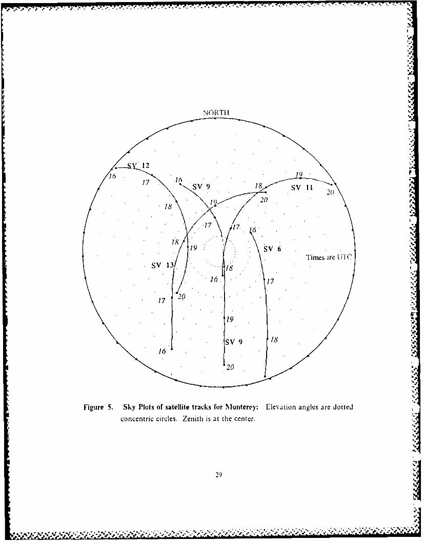
Figure 5. Sky Plots of satelIt tracks for Mlonterey........................24)
Figure 6. Mlean age of data (ephemeris).................................35
Figure 7. Difference between observation end time and 0600 PS'r........... 36Figure 8. Electron fluence........................................... 36
Figure 9. Difference in refractivity between Monterey and Sand Point.......... 38
Ficure 10. Mean M onterey- Sand Point refractivity..........................39
Figure 11. Results of station 2 offset.................................... 43Figure 12. Fraction of available triple difference observations..................44
Figure 13. Missing epochis while tracking SV 6.............................45
Figure 14. Continuous tracking without SV 6 .............................. 45Figure 15. Relative positioning geometry.................................47
vii e
MV

LIST OF SYMBOLSb Baseline distance (slope distance)
/), .Measured baseline distance
ibr True haseline distance
c Speed of light
d Day
e Elevation anolef Frequency
h Highest satellite
i Observation epoch identifier
I Integer number of epochs
1n Ref'ractivity
n,' Number of epochsn;. Number of satellites
r Receiver identifier
s Satellite identifierAngle between the vector tangent to the ellipsoid and the slope distancevector
A(r,s,i) Initial integer ambiguity
C Component or coordinate
DD(h,s.i) Double difference
E Error
E Mean error.1 ,\f Maximum number of triple difference observations
N Refractive index
SD(s.i) Single difference
TD(i) Triple difference
X X coordinate
Y Y coordinate
Z Z coordinate3(i) Difference between receiver clock times
viii
P vI. , . , , , - . - , . ,,
*,** • P ~ ~ .rv-rw~''q".,. "¢ / '*. . ,x ,,' ,,, '.'i 0 ' " *D " .- -N

V Angle between slant range '%ectors from a satellite to tw.%o ground station,;
Phase of the GPS carrier signal,
p Satellite-receiver slant rang.e
lime rate ol' chan.ce ol P
a Standard deviation
,ira~) Iropos pheric deia%
Angle between the slope distance vector and the elevation anc-le to a satel-lite
W Averagze offset of receiver clock timie
r.) Common receiver clock errors
A Difference
Ax Baseline component 'in the X direction
AY Baseline component in the Y direction
AZ Baseline component in the Z direction

LIST OF ABBREVIATIONS AND ACRONYMS
ppm parts per million
AODE Age of Data (Ephemeris)
C \ Coarse Acquisition Code
DMA Defense Mapping Agency
1)NAIITC DMA lIIdrographic Topographic Center
DOD Department of Defense
1: F Electron Fluence
GDOP Geometric Dilution of Precision
GPS Global Positioning System
Nf RY Monterev GPS antenna location
NAD83 North American Datum 1983
NGS National Geodetic Survey
NOAA National Oceanic and Atmospheric Administration
NPS Naval Postgraduate School
Ob Observin2 or observation
PDOP Position Dilution of Precision
PST Pacific Standard Time ( + 8 hours UTC
SEA-TAC Seattle-Tacoma International Airport
SPt Sand Point GPS antenna location
SV Satellite Vehicle
TDOP rime Dilution of Precision
TEC Total Electron Content
U TOW Time Of the Week
LrC Universal Coordinated Time
VLBI Very Long Baseline Interferometry
WGS84 World Geodetic System 1984
WSO National Weather Service Office
U.'
%
1. INTRODUCTION
.4 priori knowledge of the observation periods required to achieve specified orders
of Ceodetic accuracies is important in planning efticient and productive geodetic surveys.
While terrestrial Survevs have specified field and processing procedures and standards to
cate gorize the geodetic accuracies of surveys [Federal Geodetic Control Comrni.tee.
1941], only recently have standards been proposed for surveys conducted with the Global
Positioning System (GPS) [Federal Geodetic Control Conumittee, It1SO]. Among the
proposed requirements are standards for the length of observing periods and satellite
geonetry.
Field studies by Remondi [19841 and numerical simulations by Fell [1980], Langley
era!. [1984], and Landau and Eissfeller [1986] studied optinized observation periods, but
for baselines less than 100 km. Cannon et al. [19851, Bock et al. [198-41, Goad et at.
[1985]. Mader and Abell [1985], and Bertiger and Lichten [19871 conducted loP2 baseline
surveys, but did not study optimized observation periods. One of the objectives of this
thesis is to fill the gap between the above studies, i.e., exanune the optimized observatior
periods for a long baseline.
The optimized times will be examined using the correlated triple difFerence carrier
beat phase observable because of its insensitivity to integer ambiguities and loss of' lock
of the GPS carrier by the receiver. Another objective of this thesis is to add to the body.
of triple difference accuracy testing following a recommendation by Remondi [1984. p.
2591: "'More tsting is required to establish the full accuracy potential of the triple di -
ference method.
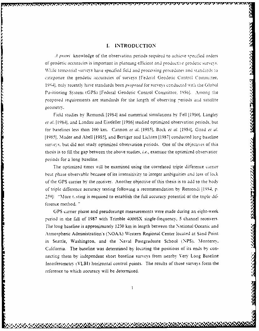
GPS carrier phase and pseudorange measurements were made during an eight-week
period in the fall of 1987 with Trimble 4000SX single-fiequency, 5 channel receivers.
The long baseline is approximately 1230 km in length between the National Oceanic and
.A\tmospheric Administration's (NOAA) Western Regional Center located at Sand Point
in Seattle, Washington, and the Naval Postgraduate School (NPS). Monterey,
California. The baseline was determined by locating the positions of its ends by con-
necting them by independent short baseline surveys from nearby Very Long Baseline
Interferometry (VLBI) horizontal control points. The results of those surveys form the
reference to which accuracy will be determined.
* '

~Additio nally, studies for repeatability were conducted following another recoz~m~en.
. dation by Remondi [1984, p. 2631 to en~hance the capabilities of GPS measurem~ents.
The reconmnendation was to perform extcnsive repeatability studies on non-\ar. mg
.-. baselines for verilking and improving the GPS modelling.
-'p
'p
5,-v
5%
I!. BASELINE DETERMINATION USING GPS
A. INTRODUCTION
The Department of Defenses IDOD) Global Positioning SN stein is intended to
provide a,-curute positioning and precise timiung for na% igation purposes by broadLastIg
codes superimposed on two radio carrier frequencies from satellites. The satellites are
* placed in a constellation so that at least four satellites are visible globally. The Precise
Code iP code) will be limited to authorized DOD users. The Coarse Acquisition (C .. )
code provides real-time accuracies to about 100 m [Baker, 19S6j and is available to
anyone.
The codes provide their transmit times, satellite orbit and clock information, and
inlormation to enable anv receiver to lock onto other GPS satellites. The orbital infor-
mation (ephemeris) provides the position of the satellite. The receiver measures the time
delay between the receipt of the C A code and its transmission time. The time delay can
be transformed into an apparent slant range from the satellite's known position to de-
ternine the location of the receiver. Since it includes delays due to receiver clock errors
and the effects of atmospheric refraction, the apparent slant range is referred to as thepseudurange. A minimum of four satellites are required to solve the system of range
equations for the receiver's coordinates and clock errors.\'While the C A code provides real-time location, it does not meet the accuracy re-
quired for precise geodetic work. Nevertheless, GPS makes possible a higher resolution
ia the carrier signal. Though the carrier itself does not contain the orbital and timing
information, which would have to be supplied by some other means, it does offer a
higher resolution because of its 19-cm wavelength
B. THE .MONTEREY-SAND POINT BASELINE
1. General
The length of the Monterey-Sand Point baseline (Figure i) was computed by
difIerencing the World Geodetic System 1984 (WGSS4) [Defense Mapping Agency,
19871 Cartesian coordinates determined for Monterey and Sand Point by short baseline
GPS surveys from known horizontal control points. The precision and agreement with
terrestrial survey results of short baseline GPS measurements using single frequency,
double difference solutions are well documented (e.g., [Remondi, 19841, [Goad and
Remondi, 19841. [Bock er al., 19841).
3
-2.5e

CJPS-
350 N+
Ora
Ca P. OR VLB
Figure 1. M~onterey-Sand Point Baseline and environs: Insets not drawni to scale.
At Sand Point, on-site meteorological measurements werc made necar the middle
of the observing session. For the Mionterey antenna determination meteorological
mecasurcfeents were made every half hour and the inean of all the measurements was
used in the processing. Trhe Tritn640 solutions were obtained using uncorrclated double
differences and estimating initial integer ambiguities. The ambiguities were fixed to the
4
1 1 1 1 ,1 1 1 1 -
VS....................S
integer values that produced the smallest residuals. A tropospheric Iactor was eltil:":ted
along with the integer ambiguities and the baseline components in th least-kquarcs
processing.
Tihe horizontal control points used for the reference stations in deternlining the
coordinates of the antennas were mobile Very Long Baseline Interferometrv (%LBI)
sites. 'fhe NADS3 Cartesian coordinates for the VLI sites were provided by the the
(iravity, Astronomy and Space Geodesy Branch of the National Geodetic Survey iNGSi
[Abell. 1987]. The NADS3 coordinates were determined in August 1987 rom a global
adjustment of VLBI surveys. Carter et al. 119851 described the NGS VLBI prograrn.
The Delernse Mapping Agency Hydrographic Topographic Office (DNIAHITC) validatedthe direct transformation of the VLBI Cartesian coordinates to WGSS4 Cartesian coor-
dinates [Kumar, 19SSI.
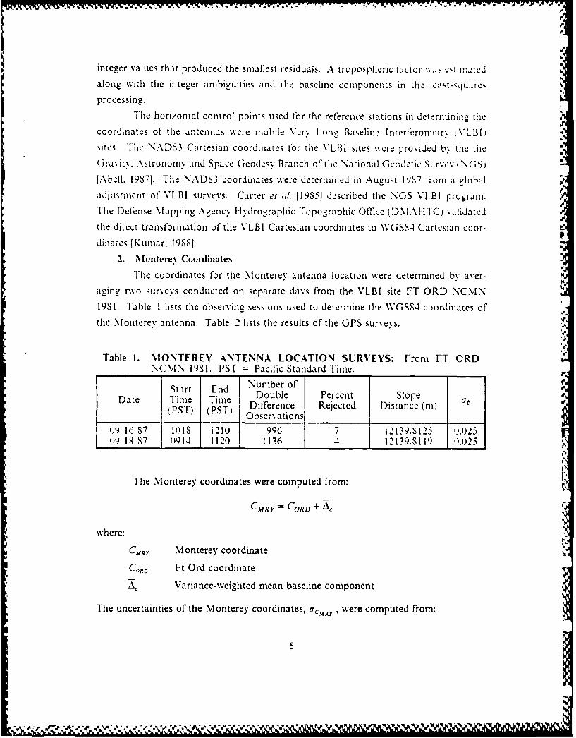
2. Monterey CoordinatesThe coordinates for the Monterey antenna location were determined by aver-
aging two surveys conducted on separate days from the VLBI site FT ORD NCMN
19S1. Table I lists the observing sessions used to determine the WGSS4 coordinates ofthe Monterey antenna. Table 2 lists the results of the GPS surveys.
Table 1. MONTEREY ANTENNA LOCATION SURVEYS: From FT ORDNCMN 1981. PST = Pacific Standard Time. _
Start End Number ofDate Time Time Double Percent SlopeDa T) 'T Difference Rejected Distance (m)(PST) (PST)Obeatn.
Observations09 16 S7 1018 1210 996 7 12139.8125 0.0250)9 18 S7 0914 1120 1136 4 12139.S119 0025
The Monterey coordinates were computed from:
C.MR = CORD + "c
where:
C.,m Monterey coordinate
C171RD Ft Ord coordinate
A, Variance-weighted mean baseline component
The uncertainties of the Monterey coordinates, ac, rY , were computed from:
5

-.V - _4 W - .... -- %.- -. v ... *. -- - .-w 7' 1~.~
Table 2. RESULTS OF MONTEREY ANTENNA LOCATION
SURVEYS: WGSS4 Cartesian Coordinates (meters).
DATE FT ORD X CORD.\ AX a~x MRY X 10Z rX
) 16 87 -2 97o)26.493 0.t)7 1 -1()313.6()l 0.032 -270734().()93 (1032,IS S7 -2o9 T26.)93 ().0()17 -11431.602 0-)37 -2707340.195 Oj37(.0.( IS -2 0 1479 -2)-,7 " ? '
Mean: -270 7340.')94 0.036
DATE FT ORD Y CORD Y AYX Y N IRY Y C.,
ok9 16 S7 -43543,93.409 0.010 9 17.693 0.048 -4353475.617 0.049()9 18 S7 -4354393.309 0.4) 917.689 0.W49 -4.3-3475.62) (1.)50
Moan: -4353475.618 0.051
DATE FT ORD Z 0ORD Z AZ Z M.MRYZ CMRYz
09 16 $7 3788},7.778 0.009 -6337.391 0.041 37S1740.387 o.042()9 IS 87 3788177.778 0.009 -6337.389 0.044 37S1740.389 0.045
.Mean: 3781740.388 0,044
2 +2
CRY = + \, a + a+
where 7,o is the uncertainty of the Ft Ord coordinate.
One month prior to the surveys originating from Ft Ord, two other surveys were
conducted from the satellite Doppler horizontal control point NAVAL POST GRAD
31965 DOPPLER. The Doppler station is approximately 300 m north of the Monterey
antenna location (Figure 1). The double differenced GPS carrier phase solutions of the
two Doppler-originating surveys yielded the following Monterey coordinates:'a
X -2707339.725 m
Y -4353475.654 m
Z 3781740.264 m
The baseline components had an uncertainty of +0.002 m, but the Doppler station has
an uncertainty of +2 m in each coordinate before transformation to WGS84. The results
of the Doppler surveys were not used in determining the Monterey coordinates because
of the large uncertainty in the Doppler station location. The three-dimensional positions
6
'P W ' V .'W"' - 4"" s V€ ''' ,
of the lonterev antenna from the Doppler and the VlBI originating suLre% 'l:rcc to
better than 0.5 m.
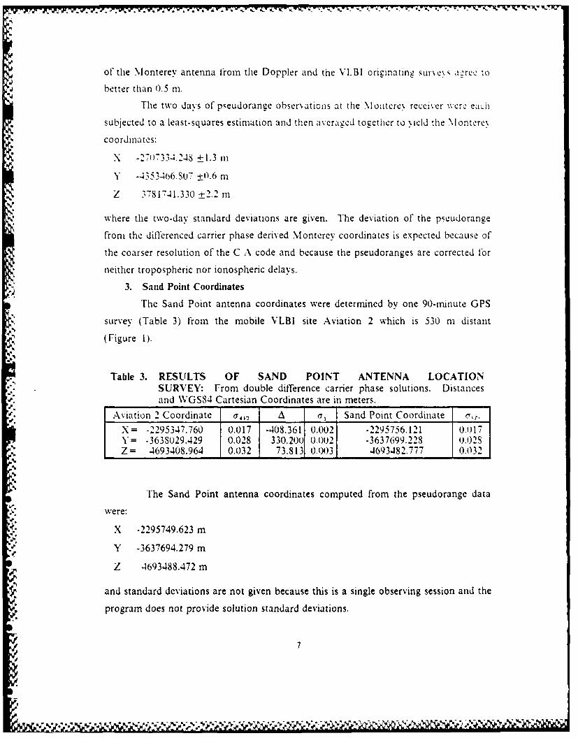
The two days of pseudorange observations at the Nlontcrey receiver were eu'.ih
subjected to a least-squares estimation and then averaged together to yteld the Monterey
coordinates:
X -27o)334.248 ±_1.3 m
Y --1353466.S07 +0.6 rn
Z 37817-41.330 -2.2 m
where the two-day standard deviations are given. The deviation of the pseudorange
from the differenced carrier phase derived Monterey coordinatcs is expected because of
the coarser resolution of the C A code and because the pseudoranges are corrected for
neither tropospheric nor ionospheric delays.
3. Sand Point Coordinates
The Sand Point antenna coordinates were determined by one 90-minute GPS
survey (Table 3) from the mobile VLBI site Aviation 2 which is 530 m distant
(Figure 1).
Table 3. RESULTS OF SAND POINT ANTENNA LOCATIONSURVEY: From double difference carrier phase solutions. Distancesand WGSS4 Cartesian Coordinates are in meters.
Aviation 2 Coordinate 0, . A (71 Sand Point Coordinate Cr.
X = -2295347.760 0.017 -408.361 0.002 -2295756.121 0.,17Y= -363S029.429 0.028 330.200 0.002 -3637699.228 0.02SZ= 4693408.964 0.032 73.813 0.003 4693482.777 0.032
The Sand Point antenna coordinates computed from the pseudorange data
were:
X .2295749.623 mY -3637694.279 m
Z 4693488.472 m
and standard deviations are not given because this is a single observing session and the
program does not provide solution standard deviations.
7
5. N.
* **.' k-A:~.%, *~%* *=*5***~**5 *S~I
I
'P
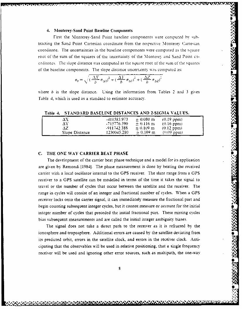
4. Monterey-Sand Point Baseline Components
First the Monterey-Sand Point baseline components were computed b% ruh-
tracting the Sand Point Cartesian coordinate from the respective Monterey CarteJan
coordinate. The uncertainties in the baseline components were computed as the square
root of the sum of the squares of the uncertainty of the MontereN and Sand Point co-
ordinates. The slope distance was computed as the square root of the sum of the squares
of the baseline components. The slope distance uncertainty was computed as:
AX" .2 A 2 AZ 2Gb = \," ( CT _I -7%1 + ( z"V,.
where b is the slope distance. Using the information from Tables 2 and 3 gives
Table 4, which is used as a standard to estimate accuracy.
Table 4. STANDARD BASELINE DISTANCES AND 2-SIGMA VALUES.
AX -411583.973 + 0.080 m (0.19 ppm)AY -715776.390 + 0.116 m (0.16 ppm)AZ -911742.388 - 0.109 m (0.12 ppm-Slope Distance 1230045.280 - 0.109 m (0.09 ppm)
C. THE ONE WAY CARRIER BEAT PHASE S
The development of the carrier beat phase technique and a model for its application -
are given by Remondi [19841. The phase measurement is done by beating the received
carrier with a local oscillator internal to the GPS receiver. The slant range from a GPS
receiver to a GPS satellite can be modelled in terms of the time it takes the signal to
travel or the number of cycles that occur between the satellite and the receiver. The
range in cycles will consist of an integer and fractional number of cycles. When a GPS
receiver locks onto the carrier signal, it can immediately measure the fractional part and
begin counting subsequent integer cycles, but it cannot measure or account for the initial
integer number of cycles that preceded the initial fractional part. These missing cycles
bias subsequent measurements and are called the initial integer ambiguity biases.
The signal does not take a direct path to the receiver as it is refracted by the
ionosphere and troposphere. Additional errors are caused by the satellite deviating from
its predicted orbit, errors in the satellite clock, and errors in the receiver clock. Anti-
cipating that the observables will be used in relative positioning, that a single frequency
receiver will be used and ignoring other error sources, such as multipath, the one-way -
8
.. ... . .S

W.- 7w .- 7.- ". V ". W ff 7
carrier beat phase, @b(r.s.i), observed at receiver, r, from satellite, s. at observation
epoch, i. can be modelled to first-order as:
Ob(r.s.i) =0,i) - Ori) - - p(rs.i)C
f I 1)+ .,,). +fr - V-bis,) 0+
- tir.i) + A~r~s.l)
vhere:
Epoch identifier
r Receiver identifier
s Satellite identifier
i Phase of received carrier signal
,5,(r,i) Phase of receiver generated carrier signal
Transnitted frequency of carrier signal
p(r.s,i) Satellite-receiver slant rangep(r,s.i) Time rate of change of slant range
c Speed of light
f Receiver generated carrier frequency
r(r,i) Tropospheric delay
,4 (r,sl ) Initial integer ambiguity
;(Ili) =i)
(2i) - (i) +
c.ti) Mean clock offset for both receivers
i(i) Clock drift between both receivers
and parentheses do not indicate factors or functions, but simply enclose identifiers.
Brackets indicate factors.
D. DIFFERENCING THE ONE-WAY CARRIER BEAT PHASE
1. Single Difference
The single difference (SD) is formed by difTerencing carrier beat phase observa-
bles from two receivers at the same observation epochs. Following Remondi [19841,
taking the difference, expanding the (ri) terms of Equation (2.1), and expressing dif-
ferences in the between-satellite and between-receiver phases as f6(i) gives:
9
le P~llp

SD(s,i) = Ot2.s.i) - P>b(l,s.i)/
m-2,3- p( I ,s.i)]
+ ". 2.s.i i(2.2)-i J2J] - AQ -JU
' ) 2.s.i) + AI .s,i) j( i)
+s[r(2,i) - r(1,i)] + A(2.s, 1) - A( I.s. 1)
where the terms are the same as Equation (2.1). Single differencing reduces or eliminates
satellite orbital and clock errors because they are common to both receivers.
2. Double Difference
A double difference (DD) is formed by differencing single differences between a
referenci.e satellite, h, and another satellite at the same epoch:
DD(h,s,i) = SD(h,i) - SD(s,i)
Because the differences at the same epoch are taken with the same reference
satellite, the double differences for each epoch are correlated. The advantage of the
double differences is that the clock dependent terms - f5(i) and [f -fj](i) - are elim-
inated. The significance of the removal of those terms is to reduce from nanoseconds
to microseconds the timing accuracy required to achieve one cicle accuracy. The
Trimble 4000SX achieves sub-nucrosecond accuracy by using the CA code tining in-
formation [Ashjaee, 19851.
3. Triple Difference
A triple difference (TD) is formed by differencing the double differences for the
same satellite pair at some integer number of succeeding epochs, I:
TD(i) = DD(h,s,i + 1) - DD(h. s,i)
The advantage of the triple difference is that it eliminates all the time inde-
pendent terms, namely the initial integer ambiguities, A(r,s,l), and becomes insensitive
to the initial ambiguities and any cycle slips when the receiver loses lock.
The disadvantages of the triple difference are: another level of correlation, loss
of resolution, and reduced number of observations. The triple differences are already
correlated with respect to satellite because of the underlying double differences, and are
10
9'.-,-,..-%%...,..;%,., ."5' '' r' ,''¢; Y -' ";6'' -:'"5",?'5 - ',:~ -
"'
further correlated with respect to time because consecutive triple dillerenced obhcr-a-
tions will have the DD(h,si + D terni in conmmon.
For short baselines, integer ambiguities can easily be resolked because unmod- belicd errors are highly correlated between the t% o antenna sites and are nostlv elinii-
nated by the differencing. Algorithms can take advantage of the integer nature of the
initial ambiguities and solve for them. At longer baselines the unmodelled errors are not
as highly correlated and not elimnated by the differencing. -liese errors fold into the
initial ambiguities, so that the ambiguities are no longer integers. In some cases the
ambiguities cannot be resolved (e.g.. Henson and Collier, 1986, Tables I and 2).
Because of the advantages the triple difference offers lor long baselines, I use the .
triple difference scheme. While the triple difference can be decorrelated by forming a
weight matrix [Remondi, 1984], only the correlated triple difference software was avail-
able to me.
E. ERROR EFFECTS
For long baseline GPS surveys, the primary errors are satellite orbit errors,
ionospheric and tropospheric delays [Remondi, 1984, and Beutler et at., 19861. Orbit
(ephemeris) errors are the result of the departure of the satellite from the broadcast
ephemeris orbit. The ephemeris is a predicted orbit for the satellite. Orbit errors prop-
agate directly into the baseline measurements when the GPS orbit coordinates are fixed
in the processing [Hothem and Williams, 1985]. Orbit errors can be the dominant error
source affecting the repeatability of long baseline measurements [Lichten and Border.
19S71.
The magnitudes of baseline errors increase with increasing baseline length because
of the increasing projection of the ephemeris error onto the baseline component [Fell,
19S0]. Estimates of the broadcast ephemeris error range from 25 m [Beutler et al.. 19S61
to 100 m [Wells et al., 1%o]. The magnitude of the effect of the ephemeris error on
baseline accuracy has been traditionally approximated [Beutler et al., 1984., Equation(2.1)]:
E ~ Eb P (2.3)b P
where:
b baseline length
p slant range (receiver to satellite)

E, error in baseline length
E, error in slant range
The slant range to a GPS satellite is about 20,000 km. which translates to a baseline er-
ror ranging froni I ppm to 4 ppm using Equation (2.3).
It is expected that the ephemeris error for the Monterey-Sand Point baseline will be
towards the lower end of the range because the ephemerides are uploaded prior to the
satellites entering the Yuma Pro ing Ground [Russell and Schaibly, 19S0J near the
California border. The ephemeris linearization error specification is to I m per day
[Wells er al., 19S61.
The ionosphere disperses the code (the group velocity) from the carrier phase (phase
velocity) because the C A code has a frequency of I Mt-Iz while the carrier signal upoll
which it is superimposed has a frequency of 1575 MHz. The effect is to increase the
pseudoranges, but decrease the carrier phase derived ranges [Smith. 1987]. Field exper-
inients [Beutler et a!., 19861 showed that ionospheric dispersion shortens baselines on the
order of a few tenths to perhaps 2 ppm.
Ionospheric error is proportional to the Total Electron Content (TEC) along the
signal path and the cosecant of the elevation angle of the satellite [Smith, 19871. Thus
the error is greatest for low elevation angles and least at the zenith. Wells et ai. [1986]
estimated that the range errors due to the ionosphere are from 150 m at the horizon to
5.) ni at the zenith.
Ionospheric activity is a function of latitude, longitude, time of day, season, and
sunspot aLtivity. Ionospheric activity increases towards the equator and towards the
sunlit portions of the earth. Diurnally, it has a minimum near 0600 local time with a
maximum around 1600 local. Ionospheric activity increases with the peak in the sunspot
cycle. The minimum in the current 11 -year sunspot cycle occurred in 19S6. Upon these
s% stematic characteristics sporadic ionospheric disturbances are superimposed.[Henson
and Collier, 1986]
The tropospheric error is proportional to the refractivity along the satellite-receiver
path and proportional to the cosecant of the elevation angle [Martin, 19801. The index
of refraction, n, is the ratio of the speed of light in a vacuum to the speed of light in a
particular medium, in this case the troposphere. Because the refractive index is a small
fraction greater than 1.0, a more convenient unit to work with is refractivity, N, where
V = (n - 1) x 106 . The magnitude of the tropospheric biases range from 20 m for 100
elevation angles to 2.3 m at the zenith [Wells et al., 1986].
12I

lenson and Collier f1986J have shown that triple difference mcasurcments are ni-
alfected by path-dependent ionospheric bias errorq, but by path-dependent cradientionospheric errors, and Martin [19S01 has estimated that the combined ionospheric andtropospheric gradient errors are on the order of meters per hour and are proportionalto the cosecant of the elevation angle.
13%
.%
I,%
-a
is
.
ba'
'a.as'a
13!
h,
a.
'a-w v ~ ~ j5a' ~ -.j~ ~ ~ ~ -~ s p ~ ~ S~f
Ill. DATA COLLECTION, PROCESSING, AND ANALYSIS
A. EQUIPMENT CONFIGURATION
1. ilardisare
A complete description of the Trinible 4u() SX receiver is gi, en bv [irnible
Navigation [(1S7a]. NPS operates three Tlimble 4(u SX GPS Surve or receivers. of
which two were used in this study. The 400oSX is capable of observing the C .\ code, ,,
integrated Doppler and carrier beat phases of up to live satellites inuitaeousiv, Its
ability to use the C A code allows the receiver to be used as a stand alone nar.:ation
system which determines position using Doppler-smoothed pseudoranges and % elocities
[AshIaee, 19851.
For precise relative positioning the 4O0QSX can transmit its data through an
RS232 port to a microcomputer for storage on floppy disk for post-processing. The4t00)SX's ability to use the C A code allows it to decode the GPS navigation rnessaces
so that it can track satellites automaticallv and determine. Most importantly. it uses the
C A code in a time transfer mode to determine any offset and drift of its own clock andthus provide accurate time tags for the observations without an external atonuc clock
or synchronization with the receiver at the other end of the baseline.
The receivers were left on continuously to allow unattended data collection. %
NIultipath-resistant Trimble microstrip antennas were installed at both the %.
Monterey and Sand Point locations.
2. Softisare
For relative positioning, the receiver is controlled from the microcomputer byVersion D of Trimble's Datalogger program. The reference position (the geodetic coor-
dinates of the antenna) and the particular options chosen must be entered into the re-
ceiver v!a the receiver keypad. The receivers were set to use the reference position height
for point positioning when less than four satellites were available.
Each observation session was initialized to log data when a minimum of four
satellites were 15* above the antenna's horizon. Five satellites were designated for each
observing session. The software logs the observables and receiver clock parameters to
a floppy disk every 15 seconds and the C A code-determined antenna position and Po-
sition Dilution of Precision (PDOP) every five minutes. The GPS navigation messageis logged to a separate file at the beginning of the session.
14
•.J•
B. SATELLITE OBSERVATION PLAN1. Satellite Selection
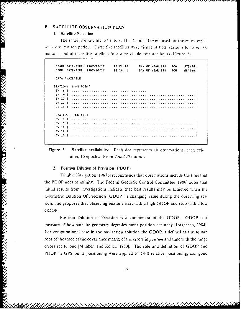
The same ti e ;atellite (SV) io. 9. 11, 12. and 13) were used for the entire e'chu-
week observation period. These flve satellites were viible at both stations lor over I(A)
nunutes. and of these live satellites four were visible for three hoUrs Figure 2 .
START DATE/TIME: 1987/10/17 15:21:15. DAY OF YEAR 290 TON 573675.
STOP DATE/TINE: 1987/10/17 18:16: 1. DAY OF YEAR 290 TON 584160.
DATA AVAILABLE:
STATION: SAND POINT
SV 6 I ...........................................SV 9 1 .... .. .. ... ... ..... .... .. ..... ... ....... .. ........ .... ... ....... .. .. .. ISV 11 I .......................................... ............................ I
$V 12 I ...................................................................... ISV 13 I ....................................................................... I
STATION: MONTEREY
SV 6 1 ....................................................
%. V 9 ...................................................................... Isv 11 I...................................................................... ISv 1 Z I .................................................. .............SV 13 I ...................................................................... I
Figure 2. Satellite availability: Each dot represents 10 observations; each ccl-
unto, 10 epochs. From Trim640 output.
2. Position Dilution of Precision (PDOP)
Irimble Navigation [1987b] reconmends that observations include the time that
the PDOP goes to infinity. The Federal Geodetic Control Conm-ittee [19861 notes that
initial results from investigations indicate that best results may be achieved when the
Geometric Dilution Of Precision (GDOP) is changing value during the observing ses-
sion. and proposes that observing sessions start with a high GDOP and stop with a low
GDOP.
Position Dilution of' Precision is a component of the GDOP. GDOP is a
imeasure of how satellite geometry degrades point position accuracy [Jorgensen, 19841.
For computational ease in the navigation solution the GDOP is defined as the square
root of the trace of the covariance matrix of the errors in position and time with the range
errors set to one [Milliken and Zoller, 1980]. The r6le and definition of GDOP and
PDOP in GPS point positioning were applied to GPS relative positioning, i.e., good
15
-b
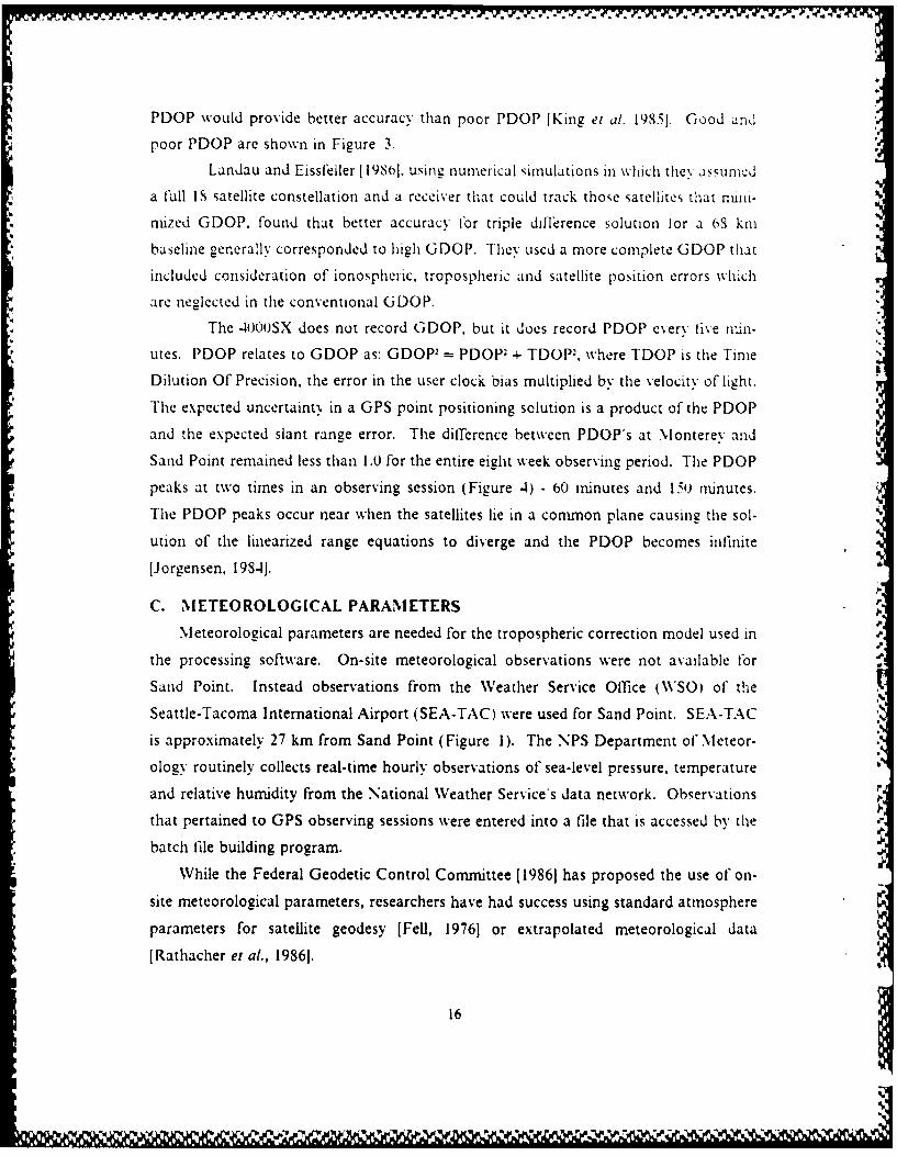
PDOP would provide better accuracy than poor PDOP [King et al. 19851. Good and
poor PDOP are shown in Figure 3.
Landau and Eissfeller [19861. usine numerical simulations in which they: assum.d
a full IS satellite constellation and a receiver that could track those satellites that nuni-
nized GDOP, found that better accuracy for triple diference solution for a 68 km
baseline generally corresponded to high GDOP. They used a more complete GDOP that
included consideration of ionospheric, tropospheric and satellite position errors which
are neglected in the conventional GDOP.
The 4000SX does not record GDOP, but it does record PDOP every five min-
utes. PDOP relates to GDOP as: GDOP2 = PDOP + TDOP2 , where TDOP is the Time
Dilution Of Precision, the error in the user clock bias multiplied by the velocity of light.
The expected uncertainty in a GPS point positioning solution is a product of the PDOP
and the expected slant range error. The difference between PDOP's at Monterey and
Sand Point remained less than 1.0 for the entire eight week observing period. The PDOP
peaks at two times in an observing session (Figure 4) - 60 minutes and 150 minutes.
The PDOP peaks occur near when the satellites lie in a common plane causing the sol-
ution of the linearized range equations to diverge and the PDOP becomes infinite
[Jorgensen, 19841.
C. METEOROLOGICAL PARAMETERS
Meteorological parameters are needed for the tropospheric correction model used in
the processing software. On-site meteorological observations were not available for
Sand Point. Instead observations from the Weather Service Office (N\'SO) of the
Seattle-Tacoma International Airport (SEA-TAC) were used for Sand Point. SEA-TAC
is approximately 27 km from Sand Point (Figure 1). The NPS Department of Meteor-
ology routinely collects real-time hourly observations of sea-level pressure, temperature
and relative humidity from the National Weather Service's data network. Observations
that pertained to GPS observing sessions were entered into a file that is accessed by the
batch file building program.
While the Federal Geodetic Control Committee [19861 has proposed the use of on-
site meteorological parameters, researchers have had success using standard atmosphere
parameters for satellite geodesy [Fell, 19761 or extrapolated meteorological data
[Rathacher et at., 19861.
16
V 1-W V4 VL^ V14,I- M ' _0 MA .- I

Jp
J.
P1
POOR POOP GOOD POOP
rigure 3. Pour and good PDOP: Fromi King et al. 11985, Fig. 3.21.
C3V
ENO.
SrA~rTSV a
*L SV a 4-
0 25 o 75 100 23 10 17
OBSEVINGTIME(min
rigur 4. DOP ersu tim
17p

...... .... . .......... 'a ,. 77777 -17777771-7777 *.17Fa a w
Hourly observations for Monterey were obtained from the NPS Department ofMeteorology. The instruments were located approximately 300 i south of the
lonterey antenna location (Figure 1).
D. PROCESSING SOFTVAREA complete description of the Trimble supplied Tritnrec software can be found in
1rimble Navigation [19S'b]. The data was processed using the Trinn-ec Frim-40 pro-gram. Revision AB. Frir.,640 limits processing to 700 epochs, so the first 700 epochs foreach observing session are used. Sand Point was used as the reference station and itscoordinates kept fixed in the least-squares processing. Sand Point was chosen as thereference station because four satellite availability occurred later at Sand Point than atMonterey. This avoided having to load the not-in-common epochs from Monterey at
each processing.
Trimn640 uses the C A code derived positions obtained at the lowest PDOP for theinitial estimates of the baseline components. Tritn640 culls the best C A code positionduring the data loading. No ionospheric correction is provided by the software, and only
the broadcast ephemeris can be used to compute fixed orbit satellite positions. In thetriple difference processing, the only parameters estimated by the least-squares process-
ing are the baseline components, AX, AY and AZ.
A modified H-opfield tropospheric model [Goad and Goodman, 19741 is used tocorrect the carrier phase delay caused by the troposphere. The correction is a functionof the atmospheric refractivity computed from surface meteorological values of pressure,temperature, and hunidity, and the elevation angle of the satellite. Larger correctionsare required for low elevation angles, as the signal travels a longer path through thetroposphere. The model corrects for at least 90% of the tropospheric delay [Remondi,19S .. Tritn640 allows only one pressure, temperature and humidity entry for each site
per session.
E. PROCESSING PROCEDURES
1. GeneralTo study optimized times, the data from each observing session were segmented.
Each successive segment contained 10 ninutes more data than its predecessor. For ex-ample, for an entire observing session that started when four satellites were available and
stopped when less than four were available provides 175 minutes of observations. Thefirst segment will use the first 10 minutes of data , the sixth segment will use the filst 60
ninutes, while the eighteenth will use all 175 minutes. For each segment, the entire
% .a
.m o - * --- . . . a i. a. ~. - - - -- - . a . . . . .. . - • a . .
".
processing was restarted from the data loading. Reloading the data for each seinent "
takes considerably longer than using the Trim640 option to flag data Ior processing. but
reloading was done so that the processing does riot use a best C A code position from
later in the observing session. -
Convergence of the least-squares solution was achieved by doing live iterations
using exery tenth triple difference formed from every tenth double difference, lbolowed
by five iterations decreasing the triple and double diflrence increneIts to live. and
finally five iterations using all triple differences forned from all double differences.
Trim640 rejects those observations whose residuals exceed a multiple of the
mean residual. The multiple of the mean residual is known as the edit multiplier.
Trim640 uses 3.5 as the default value for the edit multiplier. I used the default value for
the initial processing.
Any segment that had more than ten percent of its observations rejected or
whose solution slope distance standard deviation (a,) was greater than 10 m was re-
processed. The reprocessing was identical to the initial processing except that before I
invoking the triple difference process the pseudoranges for both stations were subjected
to separate least-squares adjustment. The pseudorange processing improves the C A
code derived initial estimates for the baseline components and corrects the carrier beat
phase time tags. The carrier beat phase time tags are computed from the C A code
times, and are earlier than the C A code times.
If the pseudorange processing failed to lower the rejections to ten percent, the .'
edit multiplier was increased until the rejections reached ten percent. A ten percent re-
jection level was observed for a few sessions and always occurred within the first thirty
inutes of observations. The data were transferred to the Naval Postgraduate School's
IBM 3033 computer for analysis. The data were analysed and graphics produced using
the APL-based GRAFSTAT program.
To study the effects of reducing observation time, five case studies were under-
taken in which the observation start times were changed fbr processing. Each case study
followed the processing procedures outlined above.
2. Batch Processing
Processing is performed in a batch mode. A batch file passes parameters to atemplate. Trimble supplies command tiles that tell the Trim640 to use the template pa-
rameters in processing.
19
I
7- W. )* -7.7-
The batch file is built using the program Bathfd (Aprendix A I. Baihid builds a
batch file by providing the appropriate file names and start and stop times. Bald/I
computes the appropriate meteorological parameters for each segment by locating the
applicable weather observations orom the weather observation lile, interpolating values
at the start time, computing running means from each hourly weather observation, theninterpolating the running means to the stop time of each segment. Two millibars wore
subtracted from the SEA-TAC sea-level pressure to compensate for the 20-rn elevation
above sea-level for the Sand Point antenna.
Initially, processing was done on an IBM XT with a math coprocessor and a
hard disk. Processing the 18 segments of an observing session took ten hours of con-
puting time. Later, processing was performed on an 80286 based mcrocomputer run-
ning at 10 .Mflz with an S0287-8 math coprocessor that reduced the processing time to
three hours.
Two minor problems with Tritn640 were discovered during the processing.
First, large values in range differences were found when using the range differences
rathcr than the pseudoranges to improve the C A code positions. The data were for-
warded to Trimble Na,,igation for evaluation and an error was found in their software.
Slhe error had no apparent effect upon carrier phase difference processing. Second, '?
Frum640 is incompatible with one or more of the AST Research, Inc. device drivers
supplied with the S0286 microcomputer: ram disk. print spooler, and extended memory,.
Removing the drivers allowed Trim640 to execute normally.
At the conclusion of the batch processing, the slope distance, the baseline
components, their standard deviations (o,1, the number of observations, the number of
observations rejected, and the RMS cycle fits were extracted from the Trim640 output,,'
file and collected into files that held the data for a particular segment for each case study.P
F. ANALYSIS PARAMETERS
The statistical parameters that will be used to evaluate the results are the error, the5-
sample mean and the standard deviation defined as [Davis et al., 1981]:
Ed= Cd- CS (5.1)
20 .
,ft.

a'--- .- E--E)
-7.7-
5517'- ,5.,.
whiere:
E, Error for day d
C, Measured component for day d
C, Expected values
E Mean error or bias
G2 Variance
G Standard deviation of F,
(Z7 Standard deviation of E
Accuracy describes the closeness between the measurements and the expected values
[Davis et al., 19811. The degree of accuracy is determined to the magnitude of the meanerror (E). The repeatability of the measurements will be expressed in terms of 2a because
it approximates the 951o confidence level for single-dimension measurements [Federal
Geodetic Control Committee, 19861. The slope distance and individual baseline con-
ponents are one-dimensional measurements.
G. DATA AVAILABILITY
Observations were made simultaneously at Monterey and Sand Point for an eight-
week period beginning 29 September 1987. Observations were made Tuesday through
Saturday except the days after federal holidays. Forty observing sessions were con-
ducted of which 2S were used in the analysis and are listed in Table 5. The remaining
12 dai s of observations were not used in the analysis for various reasons, which are
listed in Table 6.
For brevity the observing days will be referred to by their Julian day. Times in
Table 5 are given in Pacific Standard Time (PST) rather than Universal Coordinated
Time UTC) for ease in the later discussions on diurnal effects.
21
% %

Table 5. DAYS USED IN THE DATA ANALYSIS-._
Date Julian Day St lime Lid lime \umker ofSPSI) rple DatIr1
()9 29 S7 . .,33 1129 15 ) .4
Th~~~ nsI1n 1 l 5- 2- )), " 1121 1-311,, u2 57 2" (s22 I11 14-
1 3 2 '., - 1113 I1
In) uS " 2.1 ('7Iu53 5)'.
JIN o IC .3_ (14 144 1 12
1W) 14 ( 2 r32 1)2S 1 ;,2414) I $S 2'kY ( 21 1) 16 1 )4.1141 2) S7 2Q3 )'.4 1(,)2 15411 21 I.7 204 !7 95" 156211) 22 S, 21)S, i(9f)3i1S I11) 2-4 S_ 2 " 0(31 40946 14)311 27 S7 3)) 4)638 4)34 15671() 28 S7 3441 (N 3-.4 3) 151614.) 29 87 302 (q31 0926 10 ,111 03 87 3)7 1)613 ()s ISIS11 04 87 3 S )( 5 (9 )1 155311 05 87 3o9 1Th)) I.)$57 1695I1I () 87 314 0541 )837 153511 I1 7 315 11 36 U832 192711 13 87 317 ()528 ()S24 192311 1-4 87 318 )i24 )819 15,11 21 87 25 0455 750 1595112 5 87 329 1)438 0)34 1S54
Table 6. OBSERVATION DAYS NOT USED IN THE ANALYSIS.
Date Reason for not analyzing
I() 15 S7 No SEA-TAC weather observationsI[ 16 87 No satellites at Monterey for first 10 minutes10 23 87 Slope distance a, > lo m For first 10 minutes10 30 87 Disk error10 31 87 No SEA-TAC weather observations11 06 87 Unhealthy satellites11 07 87 Unhealth. satellites11 17 87 Unhealthy satellitesI I 18 87 Unhealthy satellites11 19 87 Unhealthy satellites11 2) 87 Unhealthy satellitesI 1 24 87 No satellites at Monterey for first 20 minutes
%p
22 J
-S.
Day 2S3 w'as processed with Nlonltere% as the fixed reference station because thelata set would not partition into Q-nut semnt hen Sand Point was used as tlhe
reterem~e station.
Ilie da% s that were nussing one or two segmients were excluded fromn the analy sis.
so that ii~\n the sample variances would not be dueC to unequal sample populations
het wcc:n the sea-men Cs.
Re!processiiig the first segment for 23 October failed to reduce the slope diStance
sit:n11 to less than lip m because that segment had only nine triple diflerence observa-
tion, heLause the recei'~er frequentl lost lock on the satellites. That dav was not used
in the analysis. e~ en thouzh its other segaments had slope distance sigma's less than 10
in wuizhout reprOLCsSrng.
2 3
WA.
10.

IV. RESULTS AND DISCUSSION
A. GENERAL
To ;tidk optimized times, five cases are studied:
I Process all data when four satellites at least 15" above horizon
2 Begin processing when five satellites at least 130 above the horizon
3 Begin processing as in 2. but delete fifth satellite
4 Begin processing data 40 minutes later than in 1
5 Begin processing data 70 minutes later than in I
Case I is essentially the processing of the full data set. Each of the other cases is a
subset of'Case 1. Trim640 allows the user to designate at what time within the full ob-
serxing period that the data loading should begin. For Case 3. Trun640"s ability to flag
data was used to exclude the fifth satellite (SV 12) from the processing. Each day of
Table 5 was processed for each of the live cases.
l)uring the course of the discussions it will be necessary to distinguish between ob-
servation periods and the time of the observations fixed with respect to satellite geom-
etrv. As the satellite geometry (PDOP) begins with tile availability of four satellites, the
time of observations can be defined in terms of the Case I start time. Observation pe-
riods are determined from the start time for each case. Times of observations will given
as equivalent Case I times and is obtained by adding the case observation length to the
cae s time offset from Case I (Case 2 and 3's offsets are 20 minutes Case 4., .4i) minutes
and Case 5. "0 minutes).
B. ACCURACY
1. Slope Distance
The slope distance errors for Cases 1, 2, .4. and 5 are presented in Table 7. Then
results show that accuracy to better than 1.9 ppm is achieved for any observation period,
but that there are differences among the cases and with changing observation periods
within each case.
Cases 1, 2. and .4 exhibit similar behavior as the observation period increases -
they become less positive (or more negative) as the obserxation period increases until
they reach a ninimum, then they reverse their trends and become less negative. Positive
error indicates that the measured baseline is longer than the standard values, so that the
24
* ~ 1 -v--,'

measured baselines are exhibiting an accordion effect as they shorten then iene::;en ,'p-
more observations are included in the -olutions. Wh:le the 1n11.1 O11.U1r1 ,.!ter d r1,ferent observine periods 1 1-.0. 11. ,4) minutes f,,r (ases 1, 2. and 4 respe.tI c!x .tii
occur at about the same absolute time with respect to the Case I ;tart time I 141). 13'.
and 13M minutes for Cases 1.2. and 4 respectise ). As the start times occur la:er with
eaLh caLC. the errors for shorter obser'.ing periods become less positie and tle ran.es
of the errors or each case decrease ithe range of Case 1 errors is - lo to -lS.-4 .m -.
to -IS.1 cm. for Case 2. and -1.3 to -15.1 cm, for Case 4). 1he error a!ter the entire
observation session decreases with later observing start times i -14.S cm. -9.1 cim. and
.1)-4 cm for Cases 1. 2. and 4 respectively?.
Case S behaxes imilarl% to the previous cases except that its unimum occurs
after only I0 nunutes of observations and adding more observations causes the error to
become positive. The error is largest after the entire observing session (3S.4 cm). Cases
1 2, and -4 start their observations prior to the first PDOP peak that occurs at 01) min-
utes (lieure 4) while Case 5 starts after the PDOP peak, so that starting the obsersa-
tions close to the larger PDOP peak and including the PDOP peak observations can
reduce the error and the required observaton period. The effect of the PDOP peak upon
the mean slope distance error is readily apparent in comparing Cases 4 and 5. Case 4
remains negative without the early positive error, and Case 5 remains positive as i: lacks
most of the observations from about the first PDOP peak.
The first PDOP peak at 60 minutes differs from the second PDOP peak in that %
it has a higher value, is synmetric, and occurs farther from the four satellite observation
start time than the second peak is from the four satellite observation stop time, i.e.. the
second peak occurs with lower elevation angles than the first which implies larger
tropospheric and ionospheric errors.
Ihe results for Case 3 (excluding the fifth satellite) slope distance errors are
presented in Table 8. Case 3 was studied because the Case 2 results showed a decrease
in the initial slope distance errors, and Case 3 was to study the effiects of observing five
satellites. The results show that using only four satellites makes a difference of only a
few centimeters from the results using all available satellites. It should be noted that
Case 3 uses only three satellites once SV 6 sets after 100 minutes of observations. The
Case 3 minimum, -11.5 cm, was less negative than the Case 2 minimum of -18. 1 cm.
25

Table 7. MIEAN SLOPE DISTANCE ERROR FOR CASES 1. 2.4. AND
Obser% ation Case I Case 2 Cas 4 ac5Period r
mii Icm ppm j1 cm ppmn cm 11 c ppm
0.299.4.S'.25 I6 - 2.'1
3u21." .~ -'4 -44' -12.2 rj J2 'I
4')15. 1 1.21310~ l~U ~ - 4
o. -
89-3.o -99 lT I 2~.. 4
(4-6.o) -90:1.2'.2j V1 -'2 22 ''
-4 7.S -0.96)( -16.3 -"'1 -134 7
II)-12.1 -9.)9 -13.1 -,1. 1-4 1 -11 2 ;'.'J 35 43120~ -15. -913 -I7.2 *' 14 -i 44
139 ~ - -8. -0)15 -116.7 '.3 -. )4
160) -. 0 -. 14 -9.1 -1(7 - - -
17u -15;.6 -o111'7 -1-4.8 -0.12 -.
Table S. CASE 3SNEAN ERRORS _RRRFR__SE 1._._. _____
'5,'
Observation Slope A5Period Distance
Lm pprim cm ppm cm ppm cm
In8.8 0..o7 -287i.o -6.97 177.6 2.43S -21.7 -4)243.7 9.03 -,27.') -6.0" 155.5 2.17 -15.6 -0.17
3- -0.4 -0500 -214.3 -5.21 126.3 1.76 -1.9 -"'440 -4.6 -0.04 -199.4 -S4 11 .-1 1.54 9.5 44.1-. -8.5 -0.0 -170.6 -4.15 8l.6 . 19.7 .)I
60 -10.9 -0.09 -142.2 -. 4 4.9 0.91 27.9 04.3070 -11.5 -0-10 -115.7 -2.-82 44,8 0.63 32.6 (.36So -10.1 -0.08 -9o.4 -2.11) 2-4.5 0.-34 35.1 .I'90 -10.3 -0.08 -58.7 -1.43 7.2 0.1o 34.7 0.33
100 -10.0 -0.08 -38.5 -0.95 9.2 0.13 3.7 0.26110 -10.3 -o.08 -15.8 -0.39 3.9 0.05 13.0 'Q.20120 -10.2 -0.08 5.9 0.15 -1.0 -0(.1 11.8 ).13130 -9.7 -0.08 28.7 0.70 -7.3 -0.10 5.9 04.06140 -8.8 -0.07 52.9 1.29 -18.6 -0.26 2.5 0.0175 -7.5 -0.06 737 1LSO -29.8 -0.42 0.3 00410) -5.2 -004 972 236 -45.0 -0.63 -1.5 -4.02
26
.;.. -.'40 6 9 177. . . 7 .(). 5.

2.Baseline Components
'I tie AX and AY accuracies are better than I0f.0 rpm or all obserxiniz renoulswhile AZ accuracx is better than 1 .1) ppmn lor all obser% ing period,. The acc:uracv of' tilebaseline components is expected- to be less than thle accuracY' of the baseline becauLsete
ba~cline errors are mostl% perpendic:ular to the baseilne itself- IReinondl. Il)S4!. The
baseline compornent results (Tables 14, 1o. and I I ) how that thle -1X and AY* errors are
-reater than tile baseline components M~ ille the AZ erriors are about the same order of'
niagnitude as the slope distanC en cr5. The AX anid AN' errors arc neizative~v correlated
which is the result of the correlations of the triple differences and the senmi-circular tracks
of' the satellites (Fieure . Case 3 (Table S' shio"s little difference From Case 2 In the
AX error. and a more nezati~e AY error is offset by a less necative AZ error.
The smallest mean errors for the baseline coniponents are Found at various ob-serving periods. Zero mean error for all the baseline components is achieved with fewer
observations as the observing start t imes occur closer to and before the larger PDOP
peak.
Table 9. MIEAN AX ERROR FOR CASES 1, 2. 4. AND 5 %_____
Observation Case I Case 2 Case 4 C a e 5Period
Cm1 ppm c m ppm c m PPM cmi ppmn
II0 -252.4 -6.13 -296.3 -7. 19 -136.3 -3. 30 29.o (j. 73lo-2 55.4 -6.21 -256.0 -6. 22 -136.4 -3.') S83.9 2.04
3() -2 ,55.5 -6.21 -212.1 -5.15 -107.6 ..6 2 1312.9 3.2341 -23S.0 -5. 78 -194.8 -4. 74 -80.1 -1.94 183.9 -4.47
I) -2 1.2 -5.12 -167.8 -4.08 -52.7 -1i.29 191.7 4.oo00 -197.0 -4.79 -137.4 -3.33 -24.8 -0.61 192.9 -4.69U -171.8S -4. 17 -107.3 -2.60 21.9 0.531 193.4 41.70
So -145.1 -3.52 -76.8 -1.S7 48.4 1.17 19 5.-4 4.75)o-116.9 -2.84 -31.8 -0.78 67.7 1.65 201.7 4.91
10)0 -87.3 -2.11 3.1 O.US 82.3 1.99 208. 7 5.08I11o -45.2 -1.09 28.4 0.70 96.2 2.33 221.0 5.307120 -10.7 -0. 27 48.6 1.18 112. 0 2.72 -
130 15.2 0.36 65.7 1.60 124.8 3. 0.4140 35.6 0.87 83.3 21.021 139.9 3.40 -
150 53.6 1.30 97.7 2.37 - - -
160 710. 7 1.72 110.1 2.67 - - -
170 84.3 2.04 - -
1 175 1 91.7 2.24 - - -
27

".'
Table 10. MEAN AY ERROR FOR CASES 1. 2.4. AND .
Observation Case 1 lCde 2 Case -1 Case 5Pe riod1 ""I min cm ppni cni ppm ci ppm cl ppm l
11) ISS. 2.63 199.2 2.- 11(). 1.54 9.1 (131S1.2 2.53 1 1.4 2.53 1 .6.3 1.-;9 -2s.0 -).39
30 179.3 2.50 152.4 2.13 3. 1.31 -S.6 -0I)04o 171.2 2.19 1_,9.- 1.)i "79. S 1.11 ' "
2. 153.) 2.14 125.3 15 (-(1.6 0).93 -Q2.6 -1.29141 1.97 1'.'. 1 5().-3 -91.9 -1.2"
- 127.7 1.7S 94.3 1.32 29.3 ().41 -9.7 -1.25-14.) 1.59 79.3 1.11 21.o ).30 -89.3 -1.25
94) 100 5 1.4 5S.4 Q.S2 11.1 ().16 -95.6 -1.331( 86.4 1.21 46.4 0.65 -4.() 06 - 105, . 4 - 1.4"
110 t,67 4)93 34.0 t.4 7 -3.3 -).u) -121.0 -1.o91255 S 28 23.5 0.33 -15.S -0.22 - -
130 43.3 4).64 14.S o.21 -27.7 -(.39 -_-
1404 133.9 (.47 2.9 ().1).4 -42.5 -(. 9 -
15( 25.5 ().36 -9.0 -0.13 -
10) 14.4 ).20 -17.0 -0.2- -..
170 4.0 (.406 ---17i -1. -o. 3 -".,
Table 11. MEAN AZ ERROR FOR CASES !. 2. 4. AND 5
Observation Case I Case 2 Case 4 Case 5Period[nunj cm ppm cm ppm cm ppm cm ppn,
14) -82.2 -0.90 -33.2 -03.6 -11.0 -4) 12 -l-.4 - 1920 -68.0 -0.75 -30.2 -0.33 -7.3 -44 448 -3 , ._3 -54.8 -0.60 -23.4 -0.36 -8.5 -44.)9 -2 -4 *'-
40 -47.3 -0.52 -17.0 -0.19 -8.9 -0.14) -34.S -443',-38.1 -0.42 -14.6 -0.16 -11.1 -0.12 37 - -
60 -28.9 -0.32 -12.3 -0.13 -15.1 -0.17 -39.1 -11.127() -23.8 -0.26 -ii1.6 -0.13 -15.1 -0.17 -- 4-.7 -jq .so -20.0 -0.22 -13.1 -0.14 -18.5 -).2(.) --;95 ., 4 •90 -18.1 -0.20 -12.4 -0.14 -18.9 -0.2() .'" -).5"
14t) -17.9 -0.20 -15.1 -0.17 -22.2 -) .24 -5-. -''
110 -15.6 -0.17 -15.1 -0.17 -25.7 -o.2S -56.5 -().(,2120 -17.5 -0.19 -17.2 -0.19 -27.3 -0)30) -"-
130 -16.4 -0.18 -19.8 -0.22 -28.0 -. 31140 -17.9 -0.20 -21.0 -0.23 -29.3 -0.32 -
150 -19.9 -0.22 -21.3 -0.23 -- ,160 -2).3 -0.22 -21.9 -0.24 -
170 -20.1 -0.22 ,- -'
175 -20.1 -0.22 --
284"
.4. .4%
N C)RTI I
188
16 17 1
177
19
Figure 5. Sky Plots of satellite tracks for Mionterey: Elevation angles are dotted
concentric circles. Zenith is at the center.
295

C. REPEATABILITY
I. Slope Distance
The day-to-day repeatabilities. represented as the 2e level. for Cases 1, 2. 4. and
5 are presented in Table 12, and for Case 3, in Table 13. All the cases achieve 1.1) ppm
repeatablity for any observing period except Case I which requires 20 minutes of ob-
servations. Repeatability eventually reaches better than 0.5 ppm after 60 minutes of
observations for any case.
The minimun 2a levels for all cases are reached at the So to 91) minute time of
observation, which is about 30 minutes after the larger PDOP peak. A slight increase
in the 2a level is centered about the 120 to 130 minute time of observation for all caseswhich is near the PDOP minimum, after which the 2c level decreases slightly as obser-
vations from the second PDOP peak are included in the solutions. Case 4 had the
narrowest range of 2a values, and Case I had the widest range of 2a values.
Table 12. SLOPE DISTANCE 2-SIGMA VALUES FOR CASES 1. 2. 4, AND 5Observation Case I Case 2 Case 4 Case 5
Period cm ppm cm ppm cm ppm cm ppmImini ___ ___ ____ ________ ___
10 176.8 1.44 64.8 0.53 5".S 0.47 52.0 0.4220 118.2 0.96 63.2 0.51 56.8 0.46 53.4 o.4330 84.1 4..68 58.6 0.4S 59.2 0.48 61.8 0.4q40 69.8 U.57 58.4 0.47 53.8 0.44 57.(j 0.4650 64.0 0.52 58.6 0.48 54.4 0.44 55.4 0.4560 61.8 0.50 55.2 0.45 57.6 0.47 55.0 0.4570 60.4 0.49 55.0 0.44 59.6 0.48 53.6 01.4480 57.4 0.47 56.8 0.46 60.4 0.49 53.6 0.4490 56.2 0.46 59.0 0.48 60.8 0.49 57.6 0.46
10)) 57.2 0.47 60.0 0.49 59.6 0.48 62.6 0.51110 59.2 0.48 60.4 0.49 57.8 0.47 67.8 0.55120 60.0 0.49 59.6 0.48 56.2 0.46 -130 61.0 0.50 59.0 0.48 56.0 0.46140 60.6 0.49 58.2 0.47 55.4 0.45150 60.0 0.49 57.8 - - -160 59.0 0.48 58.4170 58.6 0.48 -
175 58.6 0.43
p3
30

I
Table 13. CASE 3: 2-SIGMA VALUES
Observation SlopePeriod Distnce AX AY AZ
I min] C1 ppn C1 ppm cni ppm cm ppm ",.
10 62.4 0.51 326.o 7.92 10., 1.97 7o.6 o.8421) 59.4 0.49 30)4.2 7.3 j 135.S 1.90 8J.S 1I.S "3() 57.8 0.47 318.8 7.75 09.0 2.3o .6 1'.s441) 58.0 (0.47 (0).0 7.31 093.4 2.42 .2 0.9)
;J)5S.8 0.48 287.4 6.98 l)5.S 2.i0 )5.4 1. 4o 54.0 0.4-4 272.2 6.61 197.0 2.75 1)7.) I.0670 53.0 0.43 251.8 6.12 199.8 2,79 95.8 1.()5SO 53.6 0.44 244.6 5.94 199.4 2.79 S.) 0).9890 56.4 0.46 235.6 5.72 187.0 2.61 83.4 0.91
10) 5S. 0.47 219.8 5.34 165.8 2.32 76.2 0.8411) 59.2 0.48 199.2 4.84 13S.8 1.94 71.8 ().7912 59.0 0.48 188.8 4.59 127.4 1.78 68.2 0.75130 59.0 0.48 184.2 4.48 122.6 1.71 65.0 0.71140 58.S 0.48 IS8.4 4.58 127.2 1.7S 65.4 0.7215') 58.8 0.48 190.4 4.62 128.4 1.79 64.8 0,71160) 57.R 0.47 203.0 4-93 137.0 1.91 63.8 0.70
2. Baseline ComponentsAll the baseline components have repeatabilities better than 10.0 ppm for any
observing period except for the Case I AX, which required 20 minutes of observations
iTables 13, 14. 15. and 16).
It is interesting to note that while the AX 2a values for the first segment of
Cases 2. 3, 4, and 5 are less than Case I's first segment, the final Case 1 2a value is less
than the final segment of any other Case. The final 2a values for Cases 2, 3, 4, and 5
are greater than the Case 1 2e values after an equivalent number of observations.
The minimum 2a levels for AX and AY occur at or near the end of the observing
sessions for Cases 1,2, 4 and 5. For Case 3 the minimum 2a levels occur after 130 min-
utes of observations. The minimum AZ 2a level occurs after various observation peri-
ods, but generally in the vicinity of 130 to 150 minute observation time, which is between
the PDOP minimum and the second PDOP peak. Case 3 behaves in an opposite fashion
from the other cases in that its minimum AX and AY 2a levels occur at the 150-minute
time of observation while its AZ minimum occurs at the end of the observation period.
31
. %
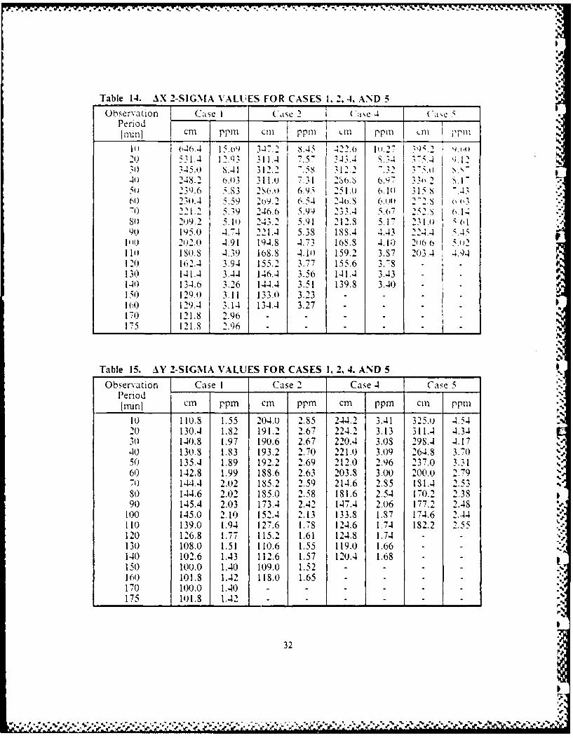
Table 14. AX 2-SIGMA VALUES FOR CASES 1. 2..4. AND 5
Observation Case I Case 2 (.ase 4 ('i,,5Period '[rai] cm ppm cm ppm -Im ppm L I ppm
11 46.4 15.o9 317.2 S.45 422.0 1"..27 .,.0 -.. .... 1o 2 5:w.2o 31.4 12.93 311.4 7.57 343.4 S.34 .4 .12
345.0 .41 312.2 312.2 ".32 -. s-248.2 6.03 311.0 7 1 2S-.- .9, 3,.2 SI
51 2301.6 5S3 2S0. 6.95 25 o1.0 .1 3 15.S -. 3360 230.4 5.59 2o9.2 6.54 24o.S 00 2"2.s o
0 221.2 5.39 246.6 5.914 23 3.4 5.67 25 14SO 2o9.2 5.1P 243.2 5.91 212.8 5.17 231 ,( 0 1"90 195.0 4.74 221.4 5.38 188.4 4.43 224.4 5.45
11) 202.0 4.91 194.8 4.73 168.8 4.1) 2(160 5 .1211) 1s0.S 4.39 168.8 4.10 159.2 3.87 203.4 4.94120 162.4 3.94 155.2 3.77 155.6 3.8 -
130 141.4 3.44 146.4 3.56 141.4 3.43 -
140 134.6 3.26 144.4 3.51 139.8 3.40150 129.0 3.11 133.0 3.23 - -
1() 129.4 3.14 134.4 3.27 - -,
170 121.8 2.96 - ,175 121.8 2.96 1,_
Table 15. AY 2-SIGMA VALUES FOR CASES 1. 2. 4. AND 5 P
Observation Case I Case 2 Case 4 Case 5Period -'
[minj cm ppm cm ppm cm ppm cm ppm-"
10 110.8 1.55 204.0 2.85 244.2 3.41 325.o 4.5420 130.4 1.82 191.2 2.67 224.2 3.13 311.4 4.3430 140.8 1.97 190.6 2.67 220.4 3.08 29S.4 4.1740 130.8 1.83 193.2 2.70 221.0 3.09 264.8 3.7050 135.4 1.89 192.2 2.69 212.0 2.96 237.0 3.3160 142.8 1.99 188.6 2.63 203.8 3.00 200.0 2.7970 144.4 2.02 185.2 2.59 214.6 2.85 181.4 2.5380 144.6 2.02 185.0 2.58 181.6 2.54 170.2 2.3890 145.4 2.03 173.4 2.42 147.4 2.06 177.2 2.48
100 145.0 2.10 152.4 2.13 133.8 1.87 174.6 2.44110 139.0 1.94 127.6 1.7S 124.6 1.74 182.2 2.55120 126.8 1.77 115.2 1.61 124.8 1.74 '--130 108.0 1.51 110.6 1.55 119.0 1.66 ,,-140 102.6 1.43 112.6 1.57 120.4 1.68150 100.0 1.40 109.0 1.52 - -
160 101.8 1.42 118.0 1.65 -"170 100.0 1.40 - -
175 101.8 1.42 "
32I

I.
f. "
Table 16. AZ 2-SIGMA VALUES FOR CASES 1. 2. 4. AND 5Observation Case I Cie 2 (ae 4 (Cae 5
Period Incm j ppm cm ppm clm ppm cn rrm
-3. 08 6i.2 (1.76 92.S 1.')2 S1.. ,S-S.O 06 73.4 h9SI S7.4 ()6 74.6 (.52
3 o s3.S ().59 o9.S ).7- S2.8 (. I ( .2 o"401 54.6 0 .) 71.6 (1.79 7S.4 l).6 57.5 .5t) 55.4 ).61 71.6 .9. 72.1) 0.-9 4').2 ' 3(,I )00.2 0.66 6S.4 ).' 68.4 0.75 47.5 . ,7() 62.6 1.09 63.3 ).70 65.0 7. 52.2,.
S61.0 ().67 59.S 0.7 .59.S .6 53.2 (..58I59.2 0.65 5S.2 (5.64 5. 2 .. 2 1.62
10) 5 .u (.).64 55.4 Q.61 53.2 0.5S 5S.2 (.64110 56.6 0.62 53.4 o.59 52.2 1.57 59.4 0(6512) 55.8 0.61 52.8 0.;S 53.6 0.-5 9130 54.4 0).60 52.4 0. S i4.0 ( ).59140 53.8 i.59 54.2 0.59 53.6 0.59150 53.6 0.59 54.4 ().61) -16) 56.) 0.61 53.4 0.59 •17) 56.6 0..62 - -
1V.5 56.0 0.61 - - .
.4
3. Standard Deviation of the Mean )
The repeatability values can be used to estimate the standard deviations of the
mean errors given in Tables 7 through II by using Equation (5.2). The values of Tables
12 through 16 should be divided by , 28 (where 28 is the sample population) to compute
the standard deviations of the means (at the 2 level). Generally, the repeatabilities were
about five times the magnitudes of the mean errors; therefore, the uncertainties of the
mean errors are on the order of the mean errors themselves. Allowing for the 0.1 ppm
uncertainty in the baseline and the baseline components and for the possible standard
deviation of the means, accuracies to better than 1.0 ppm for the slope distances and
10.0 ppm for the baseline components remain valid.
D. ERROR EFFECTS
1. 7-Day Means
Because of the observations were made over a long period of time, Case I was
subdivided into four groups comprised of seven consecutive observation days to study
trends in the slope distance error to identify the contribution of various error sources to
33
. "" N
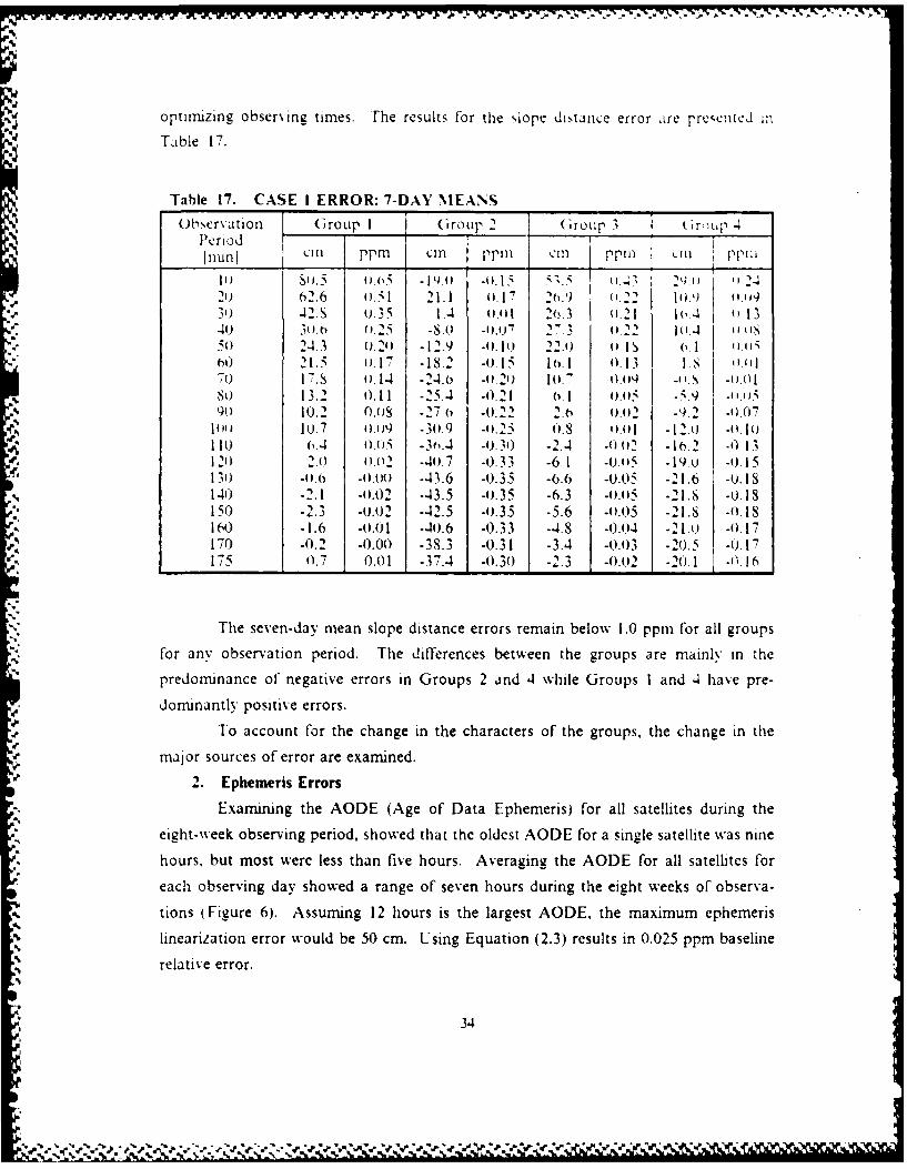
optimizing observing times. The results for the slope distance error are presented in
Table 17.
Table 17. CASE I ERROR: 7-DAY MEANS
Obhservation GroupI (iroup 2 Group 3 Or, up -Period I i
Ln1n1 rpm 1 cm ppi cm ppnrII) 54.4.5 44.6.5 -1*4.) -44.15 53.5 ''4d~ 29.n ,2420 62.6 I 21.1 0.17 2 .9 (122 10.1) 4 .q30 -12.S o.35 1.-1 .i01 26.3 1.21 1(,.. j 1 3.40 3o .25 -S.) -(oI_ 2- .3 .. 10.4 11'uS50 2-4.3 ).2) -12.9 Io.1) 22.0 ().s 6. (),o60 21.5 .17 -18.2 -0.15 16.1 0.13 I.S 0.07o 17.8 o.1.4 -24.o -or2' 1t.7 _o(I -ION -11lSO 13.2 0. 11 -25.. -o.21 6.1 (.(I5 -. 9 -4,.i1590) 10.2 0.0s -27.6 -0.2 2.( 0)02 -9.2 -0.071044 10.7 ().1)9 -3).9 -'1.25 0.S I 1. 1 -12.0 - ( I)
110 6.4 0.5 -3Th..4 -0.30 -2.4 -0).(2 -16.2 .o,13120 2.0 o.412 -4.7 -0.33 -6.1 -0.415 -19.0 -0. 15134) -o.6 .4).1) -43.6 -0.35 -0.6 -0.(15 -21.6 -O. I8141) -2.1 -o.02 -43.5 -o.35 -6.3 .).5 -21.8 -0.18150 -2.3 -U.02 -42.5 -0.35 -5.6 -. 0W5 -21.8 -0.1S160 -1.6 -o.01 -40.6 -0.33 -.4.8 -0.0.4 -21.0 -). 17170 -0.2 -0.00 -38.3 -0.31 -3.4 -0.43 -20.5 -0.17175 0.7 0.01 -37.4 -0.30 -2.3 -0.02 .20.1 -0 16
The seven-day mean slope distance errors remain below 1.0 ppm for all groups
for any observation period. The differences between the groups are mainly in the
predominance of negative errors in Groups 2 and 4 while Groups I and 4 have pre-
dominantly positive errors.
To account for the change in the characters of the groups, the change in the
major sources of error are examined.
2. Ephemeris Errors
Examining the AODE (Age of Data Ephemeris) for all satellites during the
eight-week observing period, showed that the oldest AODE for a single satellite was nine
hours, but most were less than five hours. Averaging the AODE for all satellites for
each observing day showed a range of seven hours during the eight weeks of observa-
tions (Figure 6). Assuming 12 hours is the largest AODE, the maximum ephemeris
linearization error would be 50 cm. Using Equation (2.3) results in 0.025 ppm baselinerelative error.
34
~~Z~lip,' W _. f j?~~. ~-e

II II I II ! I III T I! III 11 14 1
7-CAY YiEAN I .
272 27 8 9 0 3 2 2
a ,
27 2.79 2117 214 301 .306 315 325 32DAY
Figure 6. Mean age of data {ephenaeris)
The changes in the seven-day mean AODEs do not correspond well to the
changes in the groupings. especially as the largest change in AODE from group 3 to 4
does not correspond to a similar change in the group 3 to 4 mean slope distance errois.
his is not surprising because while the change is relatively large. the magnitude of the
orhital errors is expected to be small.
The ephemeris error will appear as a bias during any one observing session. By
averaging over eig .t weeks some of the errors will cancel and appear as variance. Be-
cause of the short observing sessions, little variation in the ephemeris error is expected
durine any single sessions
3. Ionospheric Errors
All the observing sessions completed well before 1600 local standard time and
approached the normally ionospheric activity minimum of O6)O (Figure 7). The near
north-south orientation of the Monterey-Sand Point baseline places both stations in the
same time zone, so that ionospheric errors between the two stations will be correlated
to some degree and reduced in the differencing.
35
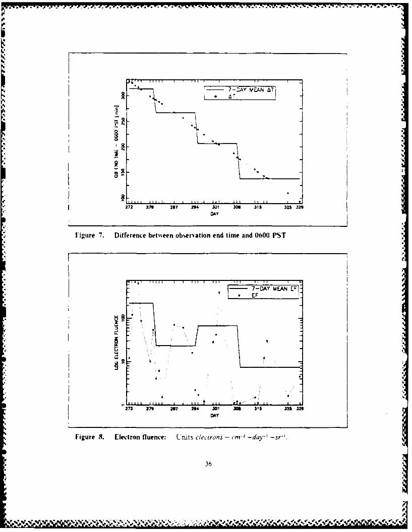
7-ZAY VEAN &T 1
Je T I 1 I f I I I I I I I I " I I " t I I
- 4A AN[l
" F.L
272 279 237 2 4 301 300 315 325 329
DAY
Figure 7. Difference beteen obsenration end time and 0600 PST
TDAYtMN EF
Il
• EF
* 36
0p
mp
- -~~ ~~q' V'v. %%!'i .(/~
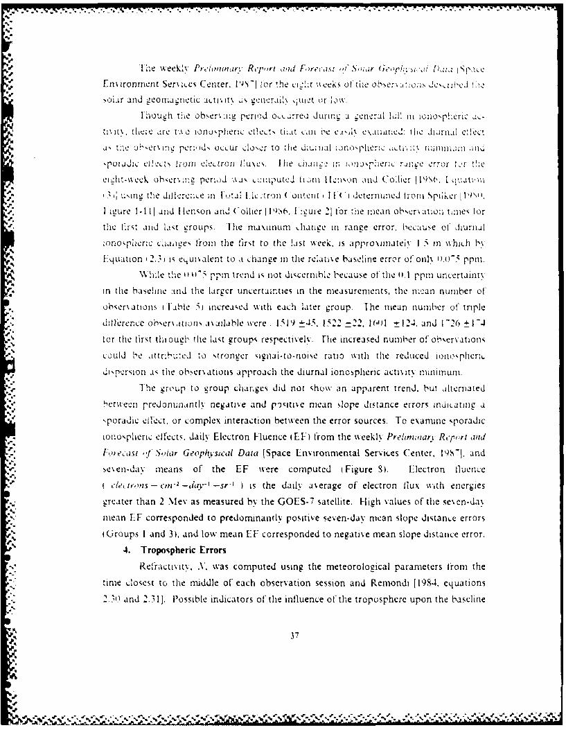
ihe weekv PreloimnarY R'l,,ri and Freca. ,,( S,),ar (.c ' sia'a I 1,
Enironment Ser,,ices Center. IV'r)S ior 'he ciht "eeks of the obthre ::os Jc',riKc t1:
SoLar and geornagnetic a 1t'.l tv as gneraU. ,it.uit or ow
Fhough the obser;.:n period o,.cirred duII- 1 .enlral lull ,I icno,.pt.L ric ,,-
t .it there arc t'o ianu,pheric Cl!ectu, tilt cii INC CA,11, C l ifmCd: thk d1rn,1l e !eCt
,is the oh-er, inc period, occ ur lo',er to the diU;iial an, io." r; 1. ti \Illflhlll i uI ti
,poladic CI 1 .t ;-011) el.. tron 1:u\CsV I he claia 1:1 on uspo erac rli e error ter the
ei-it-oeek ohser', :ri period 'ao i, Iuted I t in llicson ald Collier 1lg(O, Iquati1ii
'1 u;,ing the diliere:l .e In Futal Ilc ron (ontent - [FF ) deternined tro i Spiler I 1'9 1.
I gure 1-111 and H lenson and Collier I 19i6. I :-ure 21 for tile mean obcr-,ation nii eo tor
tile lirst and ltSt groups, The ma\iinum inhane range error, iecause of diurnal
;ono,p;iec crILes from the first to the !ast week. is appro\lwateiy 1.5 in w hJcfh by
Equation 12.3, is equi' alent to a chance in the relative baseline error olfonl% ,l w" pptn.
WhLe the I ()'5 ppm trend is not discernbhlc because of the 0. l ppm uncertainty
in tile basehine and the larger uncertainties in the measurements, the ncan number of
ohser ations iTable 5) increased with each later group. The mean number of triple
ditlerence oh~ervat.owi aailable were: 1519 .-, 1522 -22 .' 16921 . and 1-26 -V4
for the first througl the last groups respectively rile increased number of observations
could be attr-hu:ed to stronger si2nai-to-noise ratio with the reduced ionospher;c
dpersion as the obherations approach the diurnal ionospheric acti\ity miiml1"uL.
The group to group changes did not show an apparent trend. but ;ilterriated
between predonunantly negative and pgsitive mean slope distance errors indicating a
,poradic el'i;ct, or complex interaction between the error sources. To exanune sporadic
Ionospheric effects. dally Electron Fluence iEF) from the weekly Prehmnimary Rc,,prt and
Fortccast ,Y" Solar Geophysical Data [Space Environmental Services Center, 19S71, and
seen-dav means of the EF were computed (Figure S). Electron fluence
{c4'erns - cm-a y' -sr -' ) is the dally a'erage of electron flux with energies
greater than 2 Mev as measured by the GOES-7 satellite. High values of the sexen-day
mean EF corresponded to predominantly positive seven-day mean slope distance errors
(Groups I and 3), and low mean EF corresponded to negative mean slope distance error.
4. Tropospheric Errors
Reli-activit, .V. was computed using the meteorological parameters from the
time closest to the middle of each observation session and Remondi [198.4. equations
2034 and 2.311. Possible indicators of the influence of the troposphere upon the baseline
,37
laA- -- I. .

solution are the difference mn retrac:ti it'. ANY. between the bseline station,, Iand the mecan N of' both statkuns (IiL tere I' I: d,;!krCnIe La-,:iat ~ C! I
correlation of' tie troposphermc errors. (orre~aicJ tr' po,eri,: vru- tirc
Jil~eenin.The mean N (. Nwil ldli-Ite :he rMAI'litUde 01 The rei t.On c i !,,
"IOI'll to ioth sItes.
111 [he tiiL,.es IIn the dillerence in the se~ en-da' mean A I I keirc ji ki.! i
an apparent _orrespondenlce to the IIIn~ in ie Se~ el-da% group meaCn ,'lope eer rors. Instead N shows a pattern similar to the grouIp SlOpe d:'t,11nCe err1ors
ILUre 10.1Izimean rtatii-,crrcespoiided to positi% e mean slope it-Anle elrOrs
(GrouIps I and S), and low, mean refrda.tiw% ztvcmresponided \% ith negative mleanl slope
distance errors. ['he dillerence between thie high and the law mnean .\are small and do
not readilly ACcount far the nuwnitude at the .h~amzes.
7-A MA'4A
404
DAY
Figure 9. Difference in refractivity betiteen Monterey and Sand Point
38

I"S
S
U p UST
i*.
7 DAY EAjJ
272 271 2a7 314 301 306 315 325 329
DAY
Figure 10. Mean Monterey-Sand Point refractivitv
5. 7-Day Repeatability -U
The Group repeatabilities could not be given a general characterization as theI
Group means were because the was no consistent pattern to the Group-to-Group
,.hanges in their repeatabilities. For completeness. the 2e values for the various error
sources are presented in Table 18, and the Group 2c values are presented in Table 19.
Table 18. GROUP 2-SIGMA VALUES FOR THE ERROR SOURCES
Error Source Group I Group 2 Group 3 Group 4iODE 1.6 2.0 1.6 2.4
[hoursl
Observation End Time- 0600 PST 24.8 45.0 37.6 56.8kninutes]
Electron Fluence 69.[electrons - crn- -day-' -sr-J 610.0 59.6 294.8 21.4_ _.-,
27.4 21.2 27.8 23.8
- 15.2 10.6 ().0 17.8
39
,,'~U - . .., . ~ " n ", - . . . .-P .- ,- - -,, .-.- ' V,, r"v " • , " ,",' ,
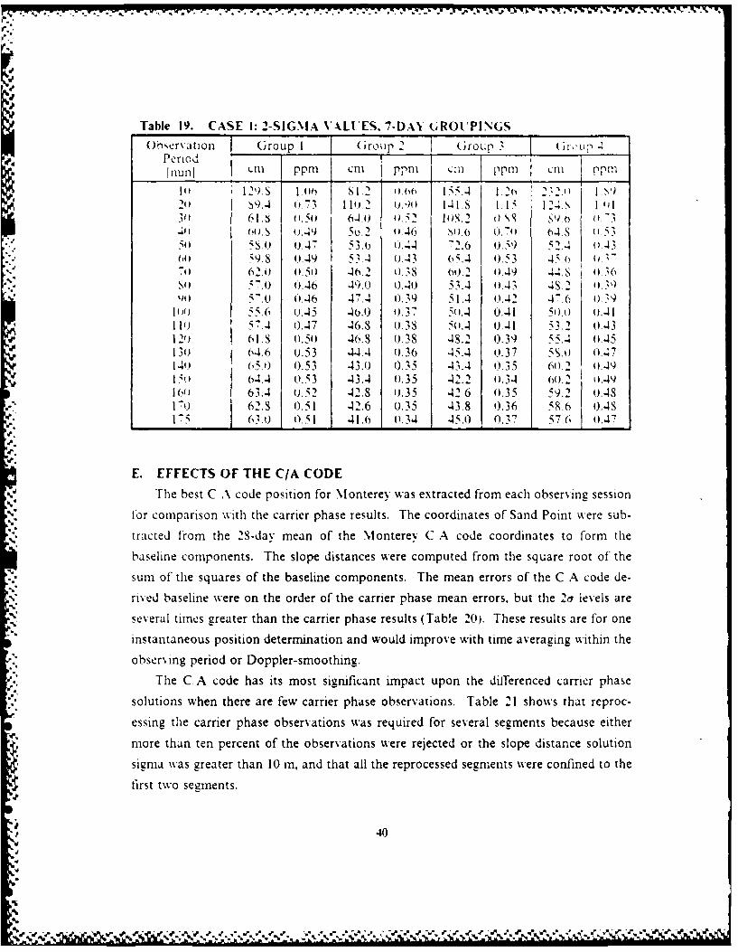
.W. v. . ~ 6 . - - -
Table 19. CASE 1: 2-SIGMIA %'XkL[ ES. 7-DAY GROUPINGSOhbser~ atioii Group I 1 rouT 2 Group 3 [ (iy-
Period ~ p m pmT ~ pm c pI mnil t}1 p i c i p n :11 p rl L1 pl
1it 129-S 1.44 8f 1.2 11.w, I1i..4 l.2 N I 4 1l..1*2'' 89.4 o.71 111.'12 (uA44 1-41.S 1.151 124.1' 141d
3061.8 N).5 6.4.0 05 10.2 44 8 s . o .44464.s 0.49 5o).2 (.46 .4, 074 o-4.S 5
;S.o ) ,.47 3.6 -.4 2.6 0.59 52.4 0464) 9. S 0.49 5.4 4143 6 5..4 0(153 4 5,~4J71) 62.0) 4). ) 46(. 2 1. 3S ('40.2 4.,49 .44.8 4 1.6
So5.;-) W.46 49.4) 0440 53. 4 (1.43 4S.2 11 19S40 'o 0.46 47.4 o.19 5 1.4 0.42 47.6) o.39
10o) 5 5.6 o.45 .4o.4)0.3 . 0.41 50)) .4 1*110 5 7.4 o.47 .46.8 (03 54.4 0)41 53.2 o..43
121) 61.S 0.50) 46.8 0J3s -1S.2 0.39 55-. 4 o.45131) 6-4.6 4)53 4.4.4 0.36 45.4 o.37 S( (o.47144.) (y-.4) 0.53 .43.0 o.)35 43.4 0).3 5 60.2 ().49
1611 63.4 o. i 42.8 oj.35 42.6 (0.35 59.2 (J.48162.8 0).51 42.6 0.35 43.8 0.36 ;8.6 j 4.4S
175 63.0 0.51 41.0 0-34 .450o 0.'7 76 o(47
E. EFFECTS OF THE C/A CODE
The best C A\ code position for Monterey was extracted from each observing session
fo r comparison with the carrier phase results. The coordinates of Sand Point were sub-
tracted from the 28-dav mean of the Monterev C A code coordinates to form the
baseline components. The slope distances were computed from the square root of the
sumn of the squares of the baseline components. The mean errors of the C A code de-
-. rived baseline were on the order of the carrier phase mean errors, but the .1C levels areseveral times greater than the carrier phase results (Table 20). These results are for one
instantaneous position determination and would improve with time averaging within the
observing period or Doppler-smoothing.
The C A code has its most significant impact upon the differenced carrier phase
solutions when there are few carrier phase observations. Table 21 shows that reproc-
essing the carrier phase observations was required for several segments because either
more than ten percent of the observations ,vere rejected or the slope distance solution
sigmia was greater than 10 m, and that all the reprocessed segments were confined to the
first two segments.
1 40
-- p V 'e 1 u
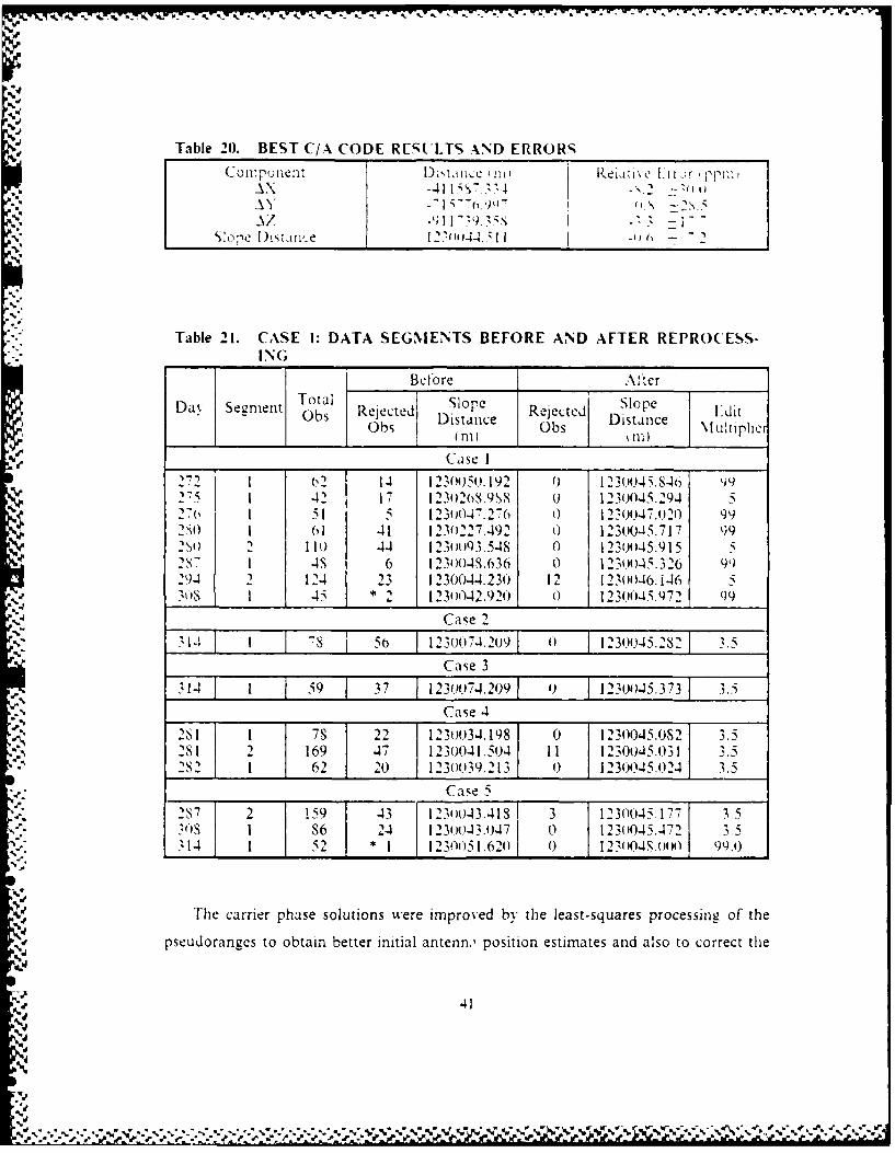
Table 20. BEST C/A CODE RESt'LTS AND ERRORS
(.owpulent l)\tlt . ,c I r 1, ',_AX -411 . 334 -\.2
_\Z -'11539.S -.33 -1- -
So ' [)0 starv.e 12.''44., f -i -
Table 21. CASE I: DATA SEGMENTS BEFORE AND AFTER REPROCESS-ING o_ _ __
_ Betore After
Day Segment Total Reetd lp Rejected S lope I'Llt)Obs DDistance liiOs Distanceultpler
_ __ _ Case l
1 6,2 14 1230050. 192 0 1230oU45.846 99-17i 1 42 17 "2 1(.I S 8 Q 230045.294 527T 1 51 5 16 0 12'0O47.020 992S( 1 61 41 1230227.492 0 1230045.717 992S1) 2 11o 44 123o()93).548 0 1230()45.915 "2S7 1 4S 6 123004S.636 0 1230045.326 9')294 2 124 23 1230044.230 12 123o0-0.1.638 1 45 * 2 123u042.920 0 1230045.972 99
Case 237I I !s 5() 123007-.2o9 0 1230045.2S2 3.5
Case 3
_314 1 59 37 1231074.209 1 ) 123o045.373 3.5
Case 4
2SI 1 78 22 123o()34.198 0 1230045.0S2 3. 5281 2 169 47 1230041.504 11 1230.45.0312S2 1 62 20 1230)039.213 0 1230045.024 3.5
Case 5
.159 43 12343.418 f 3 1230045.177 3.5T)S 1 I S6 24 123w-43.0-17 0 123(0045.472 3.5
114 1 52 * 1 230051.620 0 123(04S.000 99.0
The carrier phase solutions were improved by the least-squares processing of the
pseudoranges to obtain better initial antenn,, position estimates and also to correct the
UL %

carrier phase time-tags. All the Case I reprocessed segments were improved by f-orcing
the processing program to accept more carrier phase observations by increasing the edit
n'ultiplier.
Because of the success of improving the solutions by the pseudorange pre-
processin,. all segments for three days (276, 2S7. and 29-4) were reprocessed to see if their
already Acceptable solutions would improve. The solutions either did not change or
became slightiv less accurate.
F. COMPARISON WITH PREVIOUS STUDIES
Remondi 119S41 concluded that Ju) ppm acLuracy was achievable In () minutes and
10 ppm, in one hour - regardless of baseline length - based upon single-frequency, sinle
ditifrence solutions using precise ephemerides over baselines lcss than 100 ki. To study
the required observation times for various accuracies, he partitioned his data into
15-minute observation spans. While decorrelated triple differences would be capable ofperforming relative geodesy at I ppm level, correlated triple differences may provide 5-10
ppm or better [Remondi, 19851.
Some long baseline surveys include:
Bock et at. [19841 achieved 2 ppm accuracy in closure of a transcontinental net aidedby external atomic clocks using 10 hours of single frequency, single difference obser-vations.
Cannon et at. [1985] achieved 0.1 to 0.7 ppm repeatability using single frequencynon-dilferenced network solutions without ionospheric correction for 1700-ktn.baselines between two California stations and Calgary. Alberta. Canada over a four- rday period. The range in repeatability was attributed to satellite clock errors. T-heyalso found that the largest errors occurred in the AX component.
Mader and Abell [1985] found that single frequency long baseline GPS results usingsingle differenced carrier phase observables agreed to one ppm with VLBI measuredbaseline lengths. Their 2-day repeatability was 0.24 ppm.
Goad et a! [1985] measured a 1302-km baseline between California and Texas to betterthan 1.0 ppm compared to the VLBI measured distance, and their two-day repeat-ability was better than 0.5 ppm.
Bertiger and Lichten [1987] achieved 6 parts per billion repeatability over a 1314-km,east-west baseline over separate four and seven-day periods using dual-frequency re-ceivers with a fiducial network for orbit determination, and some water vaporradiometers.
Except for the Bertiger and Lichten [1987] results, the Case I results are competitive
with the above studies despite the inherent low resolution and the added burden of the
correlations of the correlated triple differences. A possibility for the optimum results of
Case I is that a good solution is insured by setting both receivers to their known WGSS4
42

coordinates. For real-time surveys,, one end of the baseline will USLILIV not be r1%1hJVf
to one meter accuracy. -
Durine,- the eiet-t-week obser; ation period, the thirdL A'uuSX was delivered' to MIPS.The antenna was installed on the same, rooftop, but approximately 15 in to the ner~h
of' lie NI onterev antenna. Two days Of data usHig Nonterev as the ref-rence sti* on
'.vere used :o 1Ax the loc:ation of' the newv antenna. On Dav 29-4. thc new rcceiv er c cour-
dinaes wvere oliset 3- in. eqjui~alcnt to S9Ppm baseline error. I-he di1ferenice twe
the otixet antenna and Monterey SOILUtionS for the baseline to Sand Ploint Is I7ppmn '.orthe Ii tsC-inent i iirle I I
z*
_ _ _ _ _ _ _ _ _ _ _ _ _ _ _ _ _ _ _S
CL I I I
CLa
4A 0010 6OBEVN0TM mn
Figue 11 Resltsof satio 2 ofse
For he emaiingsegentsthediferene i abot 005 pm. he irs segentwilbe mre ffeted v rceier ofse beaus thesmal nmberof arrer paseobsrva
tzn Svl esniiet h nta oiinetmt rvddb h oe h
coe intr.wl.esniietotercie1oriae ecuetercie ilcm
G.ERN MISSIE [mOCH
43/
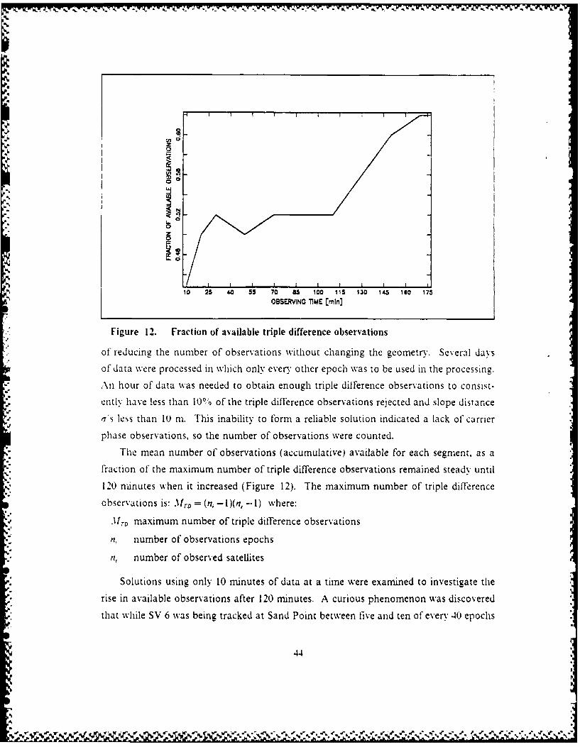
%
z
d
10 25 40 55 70 85 100 115 130 146 160 175OBSERVING TiME [mln]
Figure 12. Fraction of available triple difference observations
of reducing the number of observations without changing the geometry. Several days
of data were processed in which only every other epoch was to be used in the processing.
An hour of data was needed to obtain enough triple difference observations to consist-
ently have less than 10% of the triple difference observations rejected and slope distance
as less than 10 m. This inability to form a reliable solution indicated a lack of carrier
phase observations, so the number of observations were counted.
The mean number of observations (accumulative) available for each segment, as a
fraction of the maximum number of triple difference observations remained steady until
, 120 minutes when it increased (Figure 12). The maximum number of triple difference
observations is: -ITD = (n, - l)(n, - 1) where:
Mro maximum number of triple difference observations
n, number of observations epochs
n, number of observed satellites
Solutions using only 10 minutes of data at a time were examined to investigate the
rise in available observations after 120 minutes. A curious phenomenon was discovered
that while SV 6 was being tracked at Sand Point between five and ten of everv 40 epochs
44

were lost ( Figure 13). As soon as SV 6 was no longer being tracked at Sand Point. no
complete loss of epochs was observed I Figure 141.
ISTART DATE/TIME: 1987/10/21 16:43:07. DAY OF YEAR 294 TON 319380.
STOP DATE/TIME: 1987/10/21 16:52:b0. DAY OF YEAR 294 TCH 319980.
DATA AVAILABLE
STATION: SAND POINT
SV6 ................... ....... f.
SV 9 ...................................
SVI. I......................................
SV12 1... ................................
SV13 .........................................
STATION: MONTEREY
SV 6 1........................................................
SV 9 1 .. . . .. . .. ... . ... . .. ........ . ... . ...................
svl. ........................................................
SV1z1 .................... .............. .................
Sv13 I.......... ........................... ..................
Figure 13. Missing epochs %shile tracking SV 6: Each dot represents one obser-
vation: each colunn. one epoch. Sand Point is nussing epochs 4. 8, 14, 0
26, 30. 34, and 40. From Trim640 owput.
START DATE/TIME: 1987/10/21 17:03:04.. DAY OF YEAR 29 TON 320580.
STOP DATE/TIME: 1987/10/21 17:12:60. DAY OF YEAR 294 TON 321180.
DATA AVAILABLE
STATION: SAND POINTSV 9 .. . . .. . .. . .. . . .. . .. . . .. . .. . . .. . .. . .. . . .
SV il I .. . . .. . .. . .. . . .. . .. . . .. . .. . . .. . .. . .. . ..
SV12 ...... ..................................................
SV13 .... ............. .................. ..................
SV 61
STATION: MONTEREY
SV 1 . . . .. ... . .. .. .. . .. . . . . . . . . .. . .. . .. . . .. .Svl . .....................................................
SV12 I ................................... ..................
SV13 ........................................ ...........
SV 6 1..... ... ........ ................................
Figure 14. Continuous tracking isithout SV 6.: No missing epochs at Sand Point.
The phenomenon is not multipath interference because it affects all satellite at each
epoch. A simultaneous outage would suggest interference from some other emitter at
or near 1541) \lIIz, if the outages continued throughout the observation session rather
than being limited to when SV 6 was being tracked. No physical cause for the outages
45
-wS
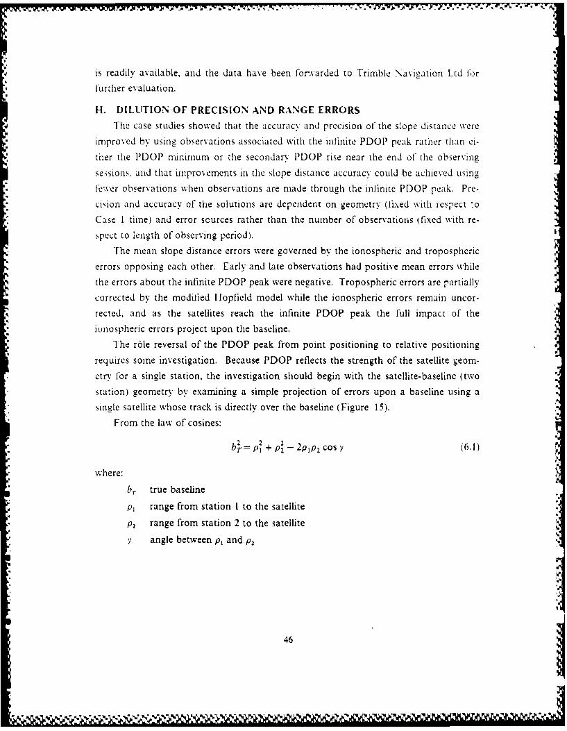
9,, . -m. ., -,,,= ,,,-.vn.¢'
, .,, , . :. . . P -J ...,.J,.t .t ft ,,,,,t ,,,,- t,. -, - '-
, . .." "P.,, J, ',' . ft.'X , .-. f t
* -
' ' - " ".
- - "-
is readily available, and the data have been forwarded to Trimble Navigation Ltd for
further evaluation.
H. DILUTION OF PRECISION AND RANGE ERRORS
The case studies showed that the accuracy and precision of the slope distance were
improved by using observations associated with the infinite PDOP peak rather than ei-
ther the PDOP ninimum or the secondary PDOP rise near the end of the observing
sessions. and that improvements in the slope distance accuracy could be achicved using
ffever observations when observations are made through the infinite PDOP peak. Pre-
cision and accuracy of the solutions are dependent on geometry (fixed vith respect :o
Case I time) and error sources rather than the number of observations (fixed with re-
spect to length of observing period).
The mean slope distance errors were governed by the ionospheric and tropospheric
errors opposing each other. Early and late observations had positive mean errors while
the errors about the infinite PDOP peak were negative. Tropospheric errors are partially
corrected by the modified H-opfield model while the ionospheric errors remain uncor-
rected, and as the satellites reach the infinite PDOP peak the full impact of the
ionospheric errors project upon the baseline.
The r6le reversal of the PDOP peak from point positioning to relative positioning
requires some investigation. Because PDOP reflects the strength of the satellite geom-
etry for a single station, the investigation should begin with the satellite-baseline (two
station) geometry by examining a simple projection of errors upon a baseline using a
single satellite whose track is directly over the baseline (Figure 15).
From the law of cosines:
bl- PI + P- 2pIp 2 cos Y (6.1)
where:
br true baseline
p1 range from station 1 to the satellite
p2 range from station 2 to the satellite
y angle between p, and P2
46
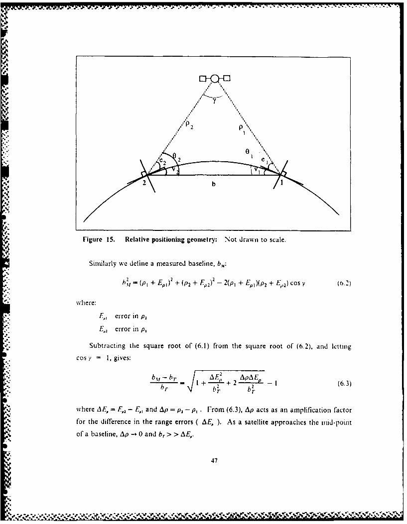
" 7 " ' W' ' W '
d: . ;'. ,-._ . -- . - -. , ltL _, ..- .p. ,, . .. . . ; . ,.-. .- ,,,, .-.-
"p
ala! Y |
2 b
Sinuilarlz we deieamasrdbslie.,
b 2|
* II
b ,=(p, + Fo,)' + (p, + F-,,)' - 2(p, + L-",)(p 2 + Et)2)co COS,2
where:
F,, error in ,
E,, error in p,
Subtracting the square root of (6.1) from th surroto(.2 adetIng
cos 1 , gives:
bN,,- b+ +f 2E ApE 2 _ 1 (6.3)
- 1+
where A E, = ,, - E,,, and Ap = p, - p, . lFrom (6.3), Ap acts as an amplification factorfor theie in the range errors AE, ). As a satellite approaches the id-poit
of a baseline, di a- 0 and br > > AE,l
4"7
= ( 1 +E,,) 2 (P +FP22-2(p + ~ 1)p2 + E,2)cosy (.2

Sirni11ar aig~urnents can be extended to point pa 'tIOi11ine U'.112 -%jiti~tsa
epochl or txo ep~sof' one sazelhte . inverting thle o~conictrn )I I i,_-ire I > Mit t ,c
reuc ian ran,_e e~rror, v' ould alppl% to point p0a tic:iine, L, %c.L
I a Ie e :'een pi'o red beca.use sz aal I ia:ni the Loiw ot : e
where 0) e . i, the ele\ aton anglc to tile satehrite and -is tlCerca anc he be-t" cell the Il'. n r C nce and tlie I o .a I ho'::on. I- \,-A ld mg sii IIt) s
"siiit' LOI, - Cos'. e',si V ,aIld sin ctCo' .1 > > ( osesi C i he .ausec o n:1 ~ is - "' to,
tile 12 31) kmi base~ine ~.then sin 0 an be approximated b\ ,in e .-\ppro\;nmatunelg~
1 23o km and p tlk 211)K kmn. then. h\ the jaw af' sinles, . is approxiniatel\ I' v% hien e is
I 3h; wThle law at' cosines, -is approximiatelyv 2.5 when thle sate!'Ilte is at the baseline
n id painlt.
With cos l>n:0.999S and cos 2.~)~9,a ven. insignificant change, most of the
deviation of- the measured baseline from the true baseline must come from the error dif-
terence factor. AE,. Most importantly has ing satellites at high elevation angles with re-
NpeCt to the ternuni of' the baseline is not detrimental to relative positioning as high %elevation angles are tar point positioning.
A second area of mx estication is tile path dependent erOrS. The Ionospheric andtropospheric errors. approximated by cosecant functions of' the elevation angle. are
minimized at hich elevation angles. Simultaneous high elevation angles for both stations
is~ another by-product of high PDOP.
Finally, the effects of differencing must be explored. Qualitatively, whenl the satel-
lites are bunchied close together at high PDOP (Figure 3), some of thle correlation in
errors that was lost in lengthening the baseline is restored. The change in tropospheric
and Ionospheric errors with time will also be miinimized because:%
d csc e -Cose d e()dt sin 2e dt
and high elevation angles minimize Equation i(6-5). Such time derivative minimization
of errors, will greatly affect the triple difference because the triple difference is itself a
timne dilference.
The sum of the elevation aneles for all satellites at both stations (Table 22) reaches
a maximum after 70 mninutes of observations, which is ten minutes later than the PDOP
L&, Z

pe-ik. The m-uinium vairtance I- achileed in the So to 94) minute111 Case I 111ne. I-he run-
nine mean of' the sumn of thie eie\ uticn ani-!e peaiks at the 1(M minute ol-er\i~
%%lite the runnig mean ele,.ut ion amiele reaL hes a local ma \111U II i te S1) to 1Ii'1i!IL1Z
I c . I hie runnling nieans provide a beter estimator ol the lreha\ :or or the Lra
1111J PreiioI1 becaulse of the accuIIJmutioI of ObSer\adtionls.
Tible 22. ELEVATION ANGLES _____ __________
OL-eration \umber FSem OfI [1-. d1in Meni 0 R1enI line a1 SVs '~s Fl\ncl Sam n
4t 511 40i- 5 4(043V S .404 5i.S .425 3
2')1' 50 54.9.43 p233' 1n55 5 2.5 .41 52.3
I)5-4, 5 -. 7 .4S6 2
00) 3t)7'9 569 50h 93~0 05o2 5 6. 2 515 4;4.2
So II)i57 j5. 52 4.410;545 4 513 ;4.4Ia53 53.5 524 ;I
11t0 I) 5 17 .51.7 523 54.1:o0 S i44 50.5 5 19 5-4.7II) s 5 ~ 5.0 516 SI)4.9
141452 56.5 5 11 55;.o01) s 441 55.1 507 55. 1
16( S418 52.3 502 55.0)I-0. s -06 594496 ~ .
494
V-
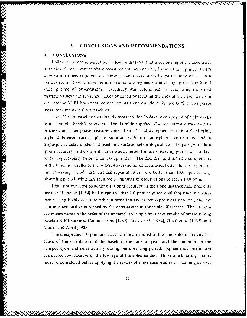
* ~ ~ ~ ~ V CO CUIN AN RECOMMENDATIONS- .. *.**, .'.~***..
4
hehnilu~,es ai reerende aun btaneodi by tocat moe estifi0the acsuroie
sery precise VLBI horizontal control points using double difference GPIS c.Irrier pilase
mneasuremients o~er short baselines.
I-le 12Sf1-kmn baseline was di.rectly measured f-or 28 da~ s o'er a period of eight weeks
Using Trimble 40041tSX receivers. The Trimble supplied Frumec software waS Used to
process the carrier phase measurements. Using broadc-ast ephemerides in a !1,,-d orbit,* triple difference carrier phase solution wkith no Ionospheric corrections and a
tropospheric dcla% model that used only surface meteorological data. 1.11 part pj:r million
ppno accuracy in the slope distance was achie~ed for any obser~ ing period with a day-
to-day repeatability better than 1.1) ppm (2a). The AX. IN', and NZ tUhe components
* . ot thme baseline parallel to the WGSS4 axes) achieved accuracies better than 111.0 ppmn for
anY obser~in,: period. AN' and AZ repeatabilities weie better than 10(.) ppmn I-or an',
oserv iii period while AX required 34) minutes of observ ations to reach 10.0 ppni.
I had not expected to achieve 1.0 ppm accuracy in the slope distance measurements
because Remondi [19841 had suggested that 1.0 ppm required dual frequency measure-
mnrts using igehly accurate orbit information and water vapor measuren --nts, and my
Solutions are further burdened by the correlat Ions of the triple differences. The 1.0 ppmi
accuracies were on the order of the uncorrelated single freqUenc% results of previous long
baseline GPS surveys: Canne-l 181 okc ! [19841. Goad ei al. [,19S51. and
Miader and Abell 119851.The unexpected 1.0 ppm accuracy can be attributed to low ionospheric activity be-
cause of the orientation of the baseline, the time of year, and the minimum in the
sunspot c~cle and solar activity during the observing period. Ephemerides errors are
considered low because of the low age of the ephemerides. Those ameliorating factors
must be considered before applying the results of these case studies to planning surveys
50
der W If
on different ba,;elnes at Jillerent times of !av and ,car. Ionospheric errors %%n cii n tu
ordcr of the tropospheric errors. -'lhe surerpoSILIOUIa 01'he CPpoS. !!on''hr_' ~ocin, n i ropospherl ic ler.gtiicn1 -Iri *e1rors redaL,.eJ mnean -iore Jista:.ic en roy
sl )Pe distance errors and ob~cr ation periud, Acere redULed A nel 0 PSOrI'er\ atlun1s
startekd niear tlie infinite. s nuiietric: PDOP peail. I LICU ed a 1 of ic ',N Or" -'c Ot t ic
1'1)01f' ;'eA k faii 1 1-c ci tt d ZO the ,,:11,11 ,,1 e - is4 1,4.1_'C.iic 0!: ia : i(rs. :11c
r:e..tioil ct' ranie eriors ama0 a hJ~cifLe1. sdte;1:c- ard Cpuii I p CiJr,1!o 11.\ii A 1I nm 1,1
() [te itele saton loec'I.r a siizle %tation can t:.,o he usckl to Ic;i; r
aL'Ile uihser',.ini tie. aI iultaneous lu.-h le,-a tioll angles correspciud to hi,-1i IP1) )l
%1% resUlts reconfirm [rii'le \as igation's I lYS7bj recommiendation to inclIUde tile
infinite PiDOP peak in the o'bsersinz session, however. I could not confirm the redeial
UcadeJtic Control Commttee s I19SO] proposal to stop at a GDOP of' 5.0. 1 could no0t
identif an% consis tent obsers mng stop point that improved accuracy other than to stop 4
%l heni four satellites were no loncer al ailabie.
When less than '() minute's of data are used. the goodness of the C A code has a
1_reat ellect upon theC carier phase solution because C A -ode positions are used to es-
ziniate thle carrier phase solution and to compute the time tags of' the carrier phiase
11meas1Urenienrs. The number of re;ected triple difference measurements pros ided the I-est
th:inLator of' thle quadlt% of' the C A code estimates and the carrier phase solutions. lIn-
cidenmces of poor accuracy of the carrier phase solution were Ibund to be caused b% poor PC A\ code estimates. The carrier phase solutions could then be improved by, correctillp
thle C A code solutions, and in turn the carrier phase time tags, by pre-processing the
C A code measurements or accepting more carrier phase measurements. Pre-processinge
the C A code measurements did not improve the accuracy of the carrier phase solutions
%%hen the numrber of rejected triple differences was less than 10%0 or when thle soILution
standard deviation of the slope distance was less than 10 m.The long-term average of the best pseudorangze solutions produced results conmpa-
rable to the mean carrier phase solution, except that the pseudorange solutions had
sariances several times the magnitude of the carrier phase solutions.
B. RECOMMNENDATIONS
The results of these case studies should be tested on surveys conducted with
baselines, of varying orientation and length arid with different satellite configurations.
51

4.
-. Currently, TRI.If 'EC does not support the use of precise ephiemcrides or zhe cor-
putation of uncorrelated triple dillerenies. Should those capchiiitlie, be :niplenntcd IIthc future, or pro% ided by third-part -olitware, the dita should he repro.esed anid In-
alvzed to isolate the tropospheric and ionosphenic error con'ributions and to improxe
the baseline component results. Both of those ..apabiities would allow !-et:er lIcht', into the el-ccts of geometry and the tropospheric and iunospheric errors.
Tfihe usual r6le of the correlated triple diflerence is to aid in fixng cicle slips ',hen" the receiver loses lock and to provide the initial estniates for the double dif erence
lcast-sqUares processing. The current data should be reprocessed in the double diller-
ence mode to determine whether the correlated triple difference solution provides sufl -
cient accuracy to fix the cycle slips and estimate the initial integer ambiguities in long
baseline sur evs.
The standard values used to estimate accuracy could be improved by a more rigor-ous fixing of the antenna locations. Both sites should be subjected to a network ad-
justment. either locally or simultaneously (possibly in conjunction with the NGS VLBI
crustal motion studies). The extra baselines required for a network solution could be
measured using the third Naval Postgraduate School receiver.
Studies should be conducted to determine the effects of using meteorological obser-
*ations far removed from the Sand Point antenna site. A temporary meteorological
station could be set up near the antenna site (possibly in cooperation with the Weather
Service Forecast Office (WVSFO) located on the grounds of the Western Regional Center
or with the nearby University of Washington). Future Naval Postgraduate School GPS
surveys would be aided by portable meteorological instruments, preferably that made
digital records of the temperature, humidity. and pressure.
Because of the importance of elevation angles to accurate results, studies should beconducted to determine the performance of the TRIM VEC supplied tropospheric mod-
els( modified Hopfield and Marini ) at various elevation angles.
While this study has shown the utility of the single-station PDOP, a more complete
DOP may provide a better satellite selection aid. Such a complete DOP ( or Dilution
Of Relative Position (DORP)) should incorporate covariances for baseline components,
satellite orbital errors, receiver timing errors, ionospheric and tropospheric delays, un-
certainties in the reference station coordinates, and cross-covariances. The DORP
would also be formulated with respect to the type of differencing to be used.
52

Lastly, the amount of' data processed for thiese case studies 'Ads hnuteJ b te -,ced
of' the microcomputer and t!he neLessItv Ot trans torrig *he re, uhs to the: \a'%, P,~ t
eraduarie School1 maintframe ta r ina~ is. As; more GTPS \%~ ~ ill !-e ccad'UtC! 111th
ILiture. the demiands for procesig rower %%ill icee.It wXil 1CLbee praie:l:
the prokxssing SOl tWare be ported to the nuin'raMle Or to a n1etwkedk itUn-cOnyuer.
Those k.0111tilers wNl1 allow multiple access to the soh w.are as %% ell as %eiee
pru.ess inu,. As an interim lneISure, the -\ NI ol tle current enseiiiile of nucrocOinput-
Or', shOUld be increased to sev eral niegab~ tes. T1his increase in R.\NI will alow the uise
ot .\ NI -dikS WhicLh %%IlI speed Up theC dc Iloaih!M UL 1hchi the nmost timeh COiisL1nu1' 1
of the processing procedures.
b
53 1

APPENDIX. BATBLD.BAS LISTING
10 REM PROGRAM BATBLD. BAS BY R. BOUCHARD NOV8720 REM PROGRAM BATBLD: BUILDS THE BATCH FILE FOR TRIMVEC PROCESSING.30 REM READS WX OHS FROM SEA. MEI FILE40 REMI DAY 283 REQUIRES ITS OWN BATBLD PROGRAM.50 INPUT "batch file name"; OFL$60 SP$5' "
70 5S$"comnand /c tbf nodd. tern80 OPEN OFL$ FOR APPEND AS #290 DIM A$(18),JD$(29),MtI$(29),DD$C29),PI!(29),PM(29)95 REM initialize Julian Day array100 JDS( 1,="272": J)$( 2) ="273": JL$( 3)="274": JD$(4)="275"
JDS(5)' 276"110 JD$( 6)='279": JD$( 7)="280": JD$(8)="281": JD$9)="282"
JD$( 10)="287" .120 JD$( 11)"290": JD$( 12)="293": JD$( 13)="294": JD$( 14)="295"-.JD$( 15 )="297" I
130 JD$( 16)='300": JD$( 17)='301": JD$( 18)="302": JD$( 19)="307",140 JD$( 20)="308": J)$( 21 )="309": JD$( 22)"3 14"145 JD(23)="3I5": JD$(24)="317": JD(25)="318"147 JD$(26)='325": JD$(27)="329" : JD$C28)='321"150 IM$( 1)='-09": MM$( 2)="09"160 FOR I=3 TO 18: MHSCI)="1O": NEXT I a
170 FOR I=19 TO 28: MM$(I)="1l": NEXT I180 DD$(l 1?"29": DD$( 2)="30": DD$( 3)="O1": DD$(4)="02": DD$(5 )='03" '
:DDS(6)= 06": DD$(7)="07": DD$( 8)="08": DD$(9)="09':. DD$( 1O)="I4":. DD$( 11)='17"
DD(12)="20"190 DD$( 13)="21": DD$( 14)="22": DD$( 15)="24':: DD$( 6)"'27": DDS( 17)='28"200 DD$( 18)="29": DD$( 19)="03": DD$(20)="04": DD$(21)="05": DD$(22)="10"205 DD$(23)="-11": DD$(24)="13": DD$(25)="14"207 DD$(26)="21": DD$(27)="25":. DD$(28)="17"210 AS( 11= a~l": A$(2)= a02 : A$(3)="a03". A$(4)="a04": A$(5)="a05":A$(6)='a06"
220 A$(7)="a07": A$(8)="a08": A$(9)="a09": A$(lO)="alO": A$(ll)"all",A$( 12)="a12" a
A$( 17)="a17": A$( 18)-"a18"240 FOR I=1 TO 7: PH(I)=19: NEXT 1250 FOR I=8 TO 13: PH(I)=18: NEXT I260 FOR I=14 TO 21: PH(I)=17: NEXT I270 FOR I=22 TO 25: PH(I)=16: NEXT I p
275 FOR I=26 TO 28: PH(I)=15: NEXT I280 PM~l)=34: PH(2)=31: PM(3)=26: PM(4)=23: PM(5)=18: PMC6)=5: PM(7)=1290 PM(8)=58: PM(9)=54: PMC1O)=33: PM(11)=22: PM(12)=8: PM(13)=3
:PM(14)=59300 PM(15)=5l: PM(16)=39: PM(17)=35: Pt(18)=31: PII(19)=14310 PMC2O)=6: PM(21)=2: PMC22)=42315 PM(23)=37: PM(24)=29: PM(25)=24: PM(26)=56: PM(27)=39: PM(28)=8317 REM begin building the batch file for each day.320 FOR 1K1l TO 28
330 OPEN "i",l,"sea.met" 54I
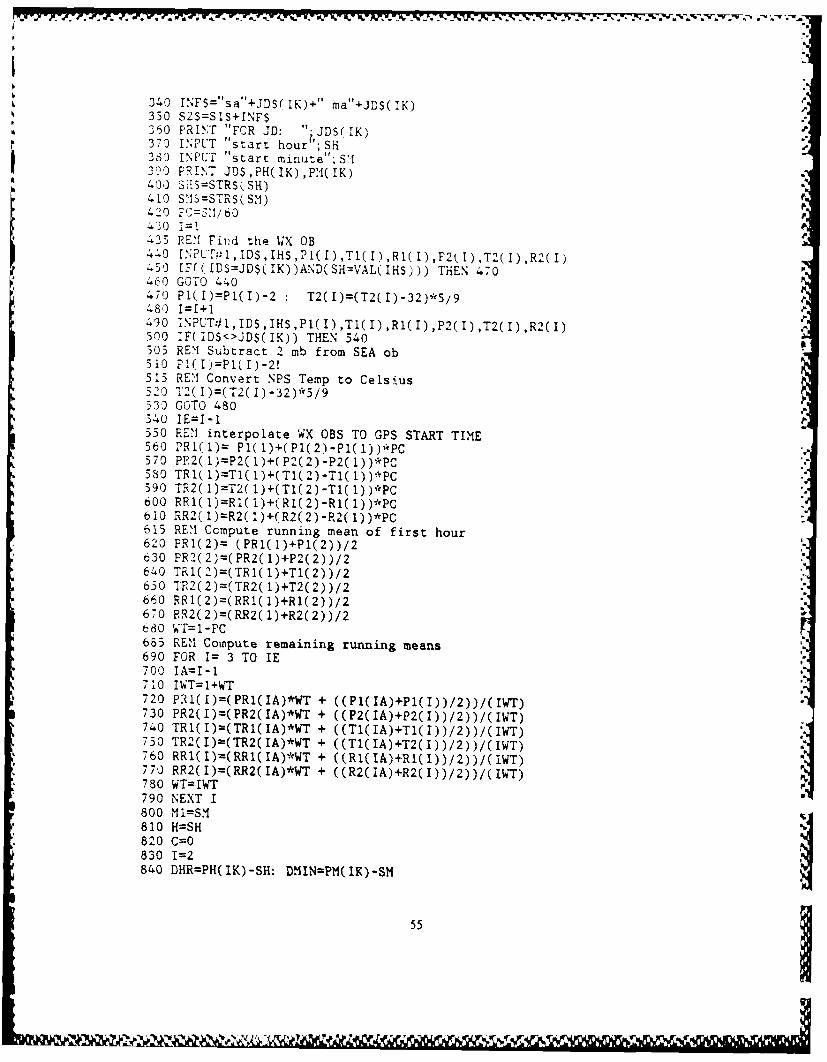
- C - - C - .
340 INF$='sa"+JDS( 'IK)+" ma"+JDS$( 1K)330 SZS=S1S+INFS
*360 PRINT "FOR TJD: "; JDS( 1K'370 I*NPUT "start hour"; SH-3680 INPUT "start minute'; SA390 PRINT JDS,PH(IK),PM-(IK)
1Ail425 FE'l Fiiud the WX 0OB
450 IF((IDS=JD$(IK))A.ND(SH=VAL(IHS))) THEN 470*460 GOTO 440
470 P1(I)=P1(I)-2 T2(I)=(T2(I)-32)*5,9483 I=I+1490 INPUT:P'l,ID$,IHS,Pl(I ),T1(I) ,Rl(I),P2(I) ,T2(I),.(I)500 IF(IDS<>JD$(IK)) THEN 540503 REMI Subtract 2 mb from SEA ob510 F1(I)=P1(IJ-2!515 RE:! Convert NPS Temp to Celsius
5Th0 T2( I )(T"(I1) -32)*5/953) COTO 480540 1E1I-l550 REM interpolate WX OBS TO GPS START TIME563) PRI(l)= Pl(l)+(Pl(2)-Pl(l))*PC570 PR,2(1)=P2(l)+(P2(2)-P2(l))*%PC580 TRl(l)=Tl(l)+(Tl(2)-Tl(l))*-PC
600 RFl(1)=Rl(!)+(Rl(2)-Rl(l))*PC610 RR2(l)=R2(1)+R2(2)-R2(l))*PC615 REM Compute running mean of first hour
630 PR2(2)=(PR2(l)+P2(2))/2640 TRl(2)=(TR1(1)+Tl(2))/2650 TR,2(2)=\(TR2(1)+T2(42))/2660 RRl(2)=(RRl(l)+R(2))/2670 RRZ2(2)=(RR2(1)+R2(2))/2680 WTF=1- PC655 REM Compute remaining running means690 FOR I= 3 TO IE700 1A=I-1710 IWT=1+WT720 Pql(I)=(PR1(IA)*WT + ((Pl( IA)+Pl(I))/2))/(IWT)730 PR2(I)=(PR2(IA)*WT + ((P2(IA)+P2(I))/2))/(IWT)740 TR1(I)=CTRl(IA)*WT + ((Tl(IA)+Tl(I))/2))/(IWT)750 TRZ(I)-(TR2CIA)*WT + ((TI( IA)+T2(I))/2))/(IWT)760 RRI(I)=(RRl(IA)*WT + ((RI(IA)+-RI(I))/2))/(IWT)770 RR2(I)=CRR2(IA)*WT + ((R2(IA)+R2(I))/2))/(IW T)780 WT=IWT790 NEXT I800 M1=SM810 H=SH
820 C=0 830 I=840 DHR=PH(IK)-SH: DMIN=PM(IK)-SM
55

850 IF(DMIN<0) THEN DHR=DHR-1: DMIN=DMIN+60860 NP=DHR*6+(DMIN/1O)865 REM Interpolate hourly running means to 10 minute intervals
*8 7-j FOR 1L=1 TO NP880 M 1=,M1+10890 IF(M1>60) THEN M1=Ml-60: H=H+l: 1=1+19 00 WT=!11/60910 IF(M1=60) THEN 41=M1-60: H=H+1: 1=1+1921) NF11I930 HP=H94.0 IWT=1-WT950 IA=I-l960 FW1=PR1(IA)*(IWT)+PRI(I)*WT
*97) PV.'= INT( ( 10'.-PW I)+. 5) /10980 PW2=PR2( IA)*( IWT)+PR2( I)*WT990 PW2=INT(( 1O*FW2)+. 5)/101000 Tlh1ITR1(IA)*(IWT)+TR1(I)*WT1010 T11INT( ( 10rTW 1) +. 5) / 101020 IV2=TR2( IA)*( IWT)+TR2( I)*WT1030 TV2=INT((1O*TW2)+. 5)/101040 RW1=RR1( IA)c( IWT)+RR1( I)*WT1050 RW1=INT((1O*RW1)+. 5)/101060 RW2=RR2(IA)p-'(IWT)+RR2(I)*WT1070 RW2=INT((1O*RW2)+.5)/101080 REM convert to strings1090 PS1$=LEFT$(STR$(PW1),7)1100 PS2S=LEFT$(STR$(PW2),7)
If 1.1110 TS1$=LEFT$(STR$(TVI),5)1120 TS2S=LEFT$(STR$(TWi2),5)1130 RS1S=LEFT$(STR$(RWI),S)1140 RS2S=LEFT$(STR$(RW2),5)1150 HSS=STR$(HP)1160 S3$=S2$+SP$+A$(IL)+". "+JD$(IK)
*1170 MS$=STRS(MP)1180 PRINT S3$+PS1$+TS1$+RS1$+PS2$+TS2$+RS2$+SP$+MM$(IK)+SP$+DDS( IK)+HSS+MS$+SH$+Stl$1190 PRINTA2, S3$+PS1$+TS1$+RS1$+PS2$+TS2$+RS2$+SP$+M1$(IK)+SPS+DDS( IK)+HS$+MS$+SH$+SM$1200 LPRINT S3$+PS1$+TS1$+RS1$+PS2$+TS2$+RS2$+SP$+MM$( IK)+SP$+DDS( IK)+HS$+MS$+SH$+SM$1210 NEXT IL1220 CLOSE #k11230 NEXT IK1240 CLOSE #A21250 END
56

REFER EN CES
Abel). %1.. National Geodetic Survey, private cominunicatiun.l.
Ashijaee, J., New reSults on the accuracv of' the C A code GPS receiver, in Proc. First
Inleptlati'na iw 'V17:0sizUf upM Precise PosavioiI with the (loba! Posliotiiag 5 t
1. 2(-)-21l4. U.S. Departmnent of Commrerce. Rock,.ille, MD, Apr. 15 to 19. 19S5.
Baker. P. J.. Global Positionfig Systemn (GPS) policy, In Pt-ac, a'ihe [Ouik Ittterih.11wzal
Geudetic s'.-nposiunm on satellite Posiriw'iag, 1, 51-04. Sponsored by tile lDefiinse
Mapping Ag~ency and the National Geodetic Survey, at Austin. TX, A\pr, _S to Mlay
2. 19S6.
Bertiger, WV.. and S. MI. Lichiten, Demonstration of 5 to 20 parts per billion repeatabihitv
for a continental baseline estimated with multi-day GPS orbits (abstraL ', EQS
Trans. .-GU. 6.3, 123S-1239, 1987.Beutler, G.. D. A. Da'idson. R. B. Langley, R. Santerre, P. Vanicek, and D. E. XWells.
Some theoretical and practical aspects of geodetic positioning using carrier phase
difference observations of GPS satellites, Tech. Rep. 109, 79 pp.. Department of'
Surveying Engineering, University of' New Brunswick. Fredericton. Canada, Jul.
iBeUtler. G., XV. Guirtner. MI. Rothacher. T. Scildkniect, and 1. Bauersima, Using the
Global Positioning System (GPS) for high precision geodetic suirveys: highlights and
problem areas, in IEEE PLA4.VS 56 Record, 243-250. Sponsored by IEEE AES So-
cietv. at Las Vegas, Nov. 4-7, 1986.
Bock. Y.. R. 1. Abbott, C. C. Counselman, S. A. Gourevitch. R. WV. King. and A. R.
Paradis, Geodetic accuracy of the Macrometer Model V-1000, Bulletin Gt~od~sique,5S, 211-221, 1984.
Cannon, E., G. Lachapelle, and C. Goad, Recovery of a 1700-km baseline using dual
frequency GPS carrier phase measurements, in Proc. First International Symposium
on Precise Positioning with the Global Positioning Sy-stetn, 11, 593-602. U.S. Depart-ament of Commrerce, Rockville, M D, Apr. 15 to 19, 1985.
Carter, WX. E.. D. S. Robertson, and J. R. MacKay, Geodetic radio interferometric sur-
veying: applications and results., Journal of Geophysical Research, 90, 4577-4587,
1985.
57LI

-- ;, .WE P.- - S - M a.. V T-a Y7PV
Davis, R. E., F. S. Foote, J. \I. Anderson. and E. M. Mikhail, Surv'eing: Ther:',, andPractice, Sixth Edition, 992 pp., McGraw-lfill, New York, 19S6.
Dellense Mapping Agency. Department of Defense World Geodetic Sisteni 198-1. D.-A
Tech. Rep. 8350.2, 121 pp.. Washington, DC. 1987.
Federal Geodetic Committee, Staldards and SpeciJ7cations f,,r Geodetic Control
.\evo)rks, 3-4 pp.. National Geodetic Information Center, NOAA. Rock-ille. MD.
19S4.
Federal Geodetic Conmittee, Proposed Geometric Geodetic Survey Standards and Spec-
iycations Jor Geodetic Surveys Using GPS Relative Positioning Techniques, 50 pp..
National Geodetic Information Center, NOAA, Rockville, MD, 1986.
Fell. P. J., The use of standard weather values and refraction bias parameters in orbit
determination, The Canadian Surveyor, 29 3,, 301-305, Sep. 1975.
Fell, P. J.. Geodetic Positioning using a Global Positioning System of satellites, Reports
of the Department of Geodetic Science, Report No. 299, 279 pp., The Ohio State Re-
search Foundation, Columbus, OH, Jun. 1980.
Goad, C. C., and L. Goodman, A modified Hopfield tropospheric refraction correction
model (abstract), EOS Trans. AGU, 55, 1106, 1974.
Goad, C. C.. and B. W. Remondi, Initial relative positioning results using the Global
Positioning System, Bulletin Geodksique, 58, 193-210, 1984.
% Goad, C. C., M. L. Sims, and L. E. Young, A comparison of four precise Global Posi-
tioning System geodetic receivers, IEEE Trans. on Geoscience and Remote Sensing,
GE-23 4,, 458-465, 1985.
Henson, D. J., and E. A. Collier, Effects of the ionosphere on GPS relative geodesy, in
IEEE PLANS 86 Record, 230-237. Sponsored by IEEE AES Society, at Las Vegas,
Nov. 4-7, 1986.
Hothem. L. D. and G. E. Williams, Factors to be considered in development of specifi-
cations for geodetic surveys using relative positioning GPS techniques, in Proc. First
International Symposium on Precise Positioning with the Global Positioning System,
II. 633-644. U.S. Department of Commerce, Rockville, MD, Apr. 15 to 19, 1985.Jorgensen, P. S., Navstar,'Global Positioning System 18-satellite constellation, in Global
Positioning System, II, 1-12. Institute of Navigation, Washington, DC. 1984.
King, R. W., E. G. Masters, C. Rizos, A. Stolz, and J. Collins, Surveying with GPS,
128 pp., School of Surveying, The University of New South Wales, Kensington,
N.S.W, Australia, 1985.
58
- ,., .
Ku~niar. M.. Defense Nlapping Agency I kdrographic IopographliL (ientcr. letter to the
author, dlated Feb. 10. 19SS.
LandULI. I I., arid B. Eis\Feller. Optimizationi of' (GPS satcilite ,eicctioii for high preciunol
dili~rential positioning, in GPS Research at thre laviiwu' I ar u'~oic Il ('1d Ph v'sical
Geoics-v. edited bvH. Landau, .13 ssfellcr. anid (. W. Hein 6i- lu), L'l1\rsr\
F.\F, Nfunich,. FRG. 19Si. r.
Langley. R. B., G. BeUtler, 1). Delikaraoizlou. B. Nickerson, R. Santerrec. P. Vanicek, a.nd
D. E. Wells. Studies in the application of' the Global Positioning Systemn to dilikr-
ential positioning. Deparitment of Survevimg Engineerig Tech. Rep. I') . 2(16 pp..
University of New Brunswick, Fredericton, Canada, 1985.
Lichten. S. )vl., and J. S. Border. Strategies for high-precision Global Positioning S% stem
orbit determination, Journal of Geophysical Research, 93, B121,, 12751-12762, Nov.
10, 1987.
Miader. G. L., and NI. D. Abell, A comparison between Global Positioning System arid
Very Long Baseline Interferometry Surveys in Alaska and Canada. in Pruc. First
International Svinposi um on Precise Positioning ivith the Global Positioning Sy stem,
11, 549-556. U.S. Department of Commerce, Rockville, MD, Apr. 15 to 19, 1985.
%Ilartin. E. H., User equipment error miodels, Global Positioning System. 1, 109-113, I n-
stitute of Navigation, WVashington, DC, 1980.
Mlilliken, R. J., and C. J. Zoller. Principle of'operation of NAVSTAR and system chiar-
acteristics, in Global Positioning System, 1, 3-14. Institute of Navigation,
Washington, DC, 1980.
Rathacher, M0., G. Beutler, and WV. Gurtner, The 1985 Swiss GPS -Campaign,in Proc.
of the Fourth International Geodetic Symposium on Satellite Positioning, 2. 979-991.
Sponsored by the Defense Mapping Agency and the National Geodetic Survey, at
Austin, TX, Apr. 28 to May 2, 1986.
Remondi, B. W., Using the Global Positioning System (GPS) phase observable for rel-
ative geodesy: modelling, processing, and results, Phi.D. Dissertation, 361 pp.. -fie
University of Texas at Austin, May 1984.
Remondi, B. W., Global Positioning System carrier phase: description and use, Bulletin
Geodesique, 59, 361-377, 1985.
Russell, S. S., and J. Ii. Schaibly, Control segment and user performance, in Global Po-
sitioning Systemn, 1, 74-10.2. Institute of Navigation, Washington, DC. 1980.
59
Smith, C, A., Ionospheric total electron content estimation for sin-gle-f-requency Global
Positioning System receivers. Ph.D. Dissertation. 11 pp., kniversitv of Ca!lfornlia,
Los Angeles. 1987.
Space Environment Services Center, PreluinarY Report and Forecast of" Solar
Geoph'sical Data, SESC PRF's 631 through 640. Boulder. CO, 06 Oct. to 08 Dec.
1987.
Spilker, J. J., GPS signal structure and performance characteristics, in Global Positioniig
Svstem, 1, 29-54. Institute of Navigation, Washington, DC. 19S0.
Trimble Navigation. Trimble Model 4000SX GPS Surveyor - PRELIAIlN,.IR Y - Instal-
lation and Operation lanual Rev. 8 1 87, 96 pp., Sunnyvale. CA, 19S7a.
Trimble Navigation, TRIMV EC GPS Survey Sojtware Preliminary User's Manual,
Rev. B, 62 pp., Sunnyvale. CA, 1987b.
Wells, D. E. (Ed.). Guide to GPS Positioning, Canadian GPS Associates, Fredericton,
New Brunswick, Canada, 1986.
I60
PA
'II
60 60
4
INITIAL DISTRIB3UTION Lisr
\a. Copies
i. lpeiene echnical lnfornxion CenterCamieron Station.\ie\aidria. VA 223(W4,1-45
2. LihrarY. Code 01-421\aval PostoLradkujte SchoolMlonterey, C:A 939-43-501)
3. Chiman jCode 6SCo)Diepartmenot of OceanographyNa~ al Postg~raduate School\Iontere%, CA 93943
4. Prof Stevens P. '[ucker 31)epartnient of Oceanographyv (Code 68Tx)Naval Postizraduate SchoolMlonterey, CA 939-43
S . Prof Narendra K. Saxena 3Department of Civil Engineering
-~ 1niversitv of Ilawaji at ManoaW% 2,540 Dole Street. Holmes 3S3
Honolulu, HI 96822
6. LT Richard H. Bouchard. USN 3NAVOCEANCOMCEN JTWCCOMSvNAVMIARIANAS Box 12FPO San Francisco966310-2926
7. Dircctor Naval Oceanography DivisionNaval Observatory34th and Mvassachusetts Avenue NWWashington, DC 20390
8. CommnanderNaval Oceanography Comm-andNSTL StationBay St. Louis, MS 39522
9. Commanding OfficerIA Naval Oceanographic Office
NSTL StationBay St. Louis, MS 39522
61
. . . . .
Iv,1 Q 4 , 1 o r ,r 11111111 11N.-A ,1. .A .

10. Commianding, OfficerNav-al Ocean Research and Development AtvtNSTL StationBar St. Louis. NIS 39522 b
11. Chairman. Oc.eanographiy DepartmentIU .S. N\aval Acadenn'Annapolis. MID 21-4o2
12. Chief of'Nav-al Research (Code 420) 1Naval Ocean Research and Deveiopmient Activity,SIA) N. QUIncy StreetArhinvon. VA 22127
13. Director i Code PPH)Defense Mapping AgencyBld2. 56. L.S. NavalObservatoryWashington. DC 200305
14. Director (Code U10) rDefense MIapping .Agency 11ydrographic, Topographic Centerr6300)I B~rookes Lane J
Washington. DC 20315
15. Director (Code PSD-NIC) IDefense Mapping SchoolFt. Belvoir, VA 22060
16. Director, Charting and Geodetic Services (N, CG) SNational Ocean and Atmospheric Administration 5
Rockville, MD 20852
17. Chief, Program Planning, Liaison and Training (NC2)National Oceanic and Atmospheric AdministrationRockville, MD 20852
18. LTJG James Waddell, NOAAISMIC 2590Naval Postgraduate SchoolMonterey. CA 93943
19. Mr. Gary Fredrick1NOAA, NOSCode N'MOP 222Bin C157007600 Sand Point Way, NESeattle, WA 98115-0070
20. Mfr. Paul PerraultITrimble Navigation, Ltd.585 North M~arv AvenueSunnyvale, CA 94088-3642
62
S\Ic 2221)Nalal 1PotcraJuace School\Iontercy, CA: 1)3943;
22. D~r. Stephen MI. LidhtenIJ1et Prouukil Lahorator,
(a tor ' u t f 1 e i n l
4Y911 Ujk' (Jio~ Drie
Pa,,adna. C 9 11
63 V

A *-* **-~-~- - -~ -.-
0
"A
"I'S
.1*
5%5%
Si-.. w~Y t-
,p% ~.rV
u~k
S.5 'p
~- U-.'
U..U- is
i.~'. b5%
.
S*5 - 5S 4* ffU
HE
S'p
'p UU
'p U
U 1~IS
U
w w w w w w w w w S- '~ .is~* 'w U',