Emotions in Macroeconomic News and their Impact on

the European Bond Market

Sergio Consoli∗ Luca Tiozzo Pezzoli† Elisa Tosetti‡

This version: March, 2021.

Summary

We show how emotions extracted from macroeconomic news can be used to explain and forecast future behaviour of sovereign

bond yield spreads in Italy and Spain. We use a big, open-source, database known as Global Database of Events, Language

and Tone to construct emotion indicators of bond market affective states. We find that negative emotions extracted from

news improve the forecasting power of government yield spread models during distressed periods even after controlling for the

number of negative words present in the text. In addition, stronger negative emotions, such as panic, reveal useful information

for predicting changes in spread at the short-term horizon, while milder emotions, such as distress, are useful at longer time

horizons. Emotions generated by the Italian political turmoil propagate to the Spanish news affecting this neighbourhood

market.

Keywords: Sovereign bond yield spreads, news, text analysis, emotions extraction, GDELT.

JEL classification: G12, G17, E43

The views expressed are purely those of the writers and may not in any circumstance be regarded as stating an official position

of the European Commission. The authors declare that there is no conflict of interest that could be perceived as prejudicing

of the research reported. This research did not receive any specific grant from funding agencies in the public, commercial, or

non-for-profit sectors.

∗European Commission, Joint Research Centre, Directorate A - Strategy, Work Programme and Resources, Scientific Devel-opment Unit, Via E. Fermi 2749. I-21027 Ispra (VA), Italy [E-mail: sergio.CONSOLI@ec.europa.eu].

†Corresponding author: European Commission, Joint Research Centre, Directorate A - Strategy, Work Programmeand Resources, Scientific Development Unit, Via E. Fermi 2749. I-21027 Ispra (VA), Italy [E-mail: luca.TIOZZO-PEZZOLI@ec.europa.eu]

‡Ca Foscari University, Italy [E-mail: elisa.tosetti@unive.it].

1

arX

iv:2

106.

1569

8v1

[ec

on.G

N]

15

Jun

2021

1 Introduction

The turbulence in government yield spreads observed since the intensification of the financial crisis in 2009

in countries within the Euro area has originated an intense debate about the drivers of the sovereign bond

market. Traditionally, factors such as public debt sustainability, liquidity of sovereign bonds, and global

risk aversion as well as other macroeconomic variables like countries’ GDP growth and inflation have been

indicated as important determinants of government yield spreads. Recently, an emerging literature having

its roots in behavioural finance points at human perception, instinct and sentiment of investors as important

elements that may guide their judgement and decision making, ultimately impacting their investment deci-

sions (Blommestein et al. (2012)). To account for these factors, recent studies propose to measure sentiment

from pieces of text such as news, blogs and other forms of written communication and use it to model and

predict developments in the financial market (Tetlock (2007), Garcia (2013)). News often contain unan-

ticipated information about the state of the economy in the form of description of the state of markets,

comments on their evolution or about possible interventions in monetary policy. Through the lenses of news

articles, market participants learn about recent economic events and trends, and adjust their perception

and expectations on the dynamics of financial markets. A number of studies extract sentiment indicators

from news and use it to model and forecast sovereign bond spreads (see, for example, Liu (2014), Apergis

(2015), and Bernal et al. (2016)). These works calculate their sentiment measures by looking at how many

positive and negative words can be found in the text according to a predefined lexicon, such as the Loughran

and McDonald (2011) word lists. Empirical findings provide evidence that news’ sentiment conveys useful

additional information over quantitative financial data for predicting government yield spreads.

In this paper we extend this line of inquiry by focusing on emotions extracted from macroeconomic

news and their role in anticipating movements in sovereign bond spreads. Emotions, or affective states, are

responses to interpretation and evaluation of events and hence reveal useful information about investors’s

behaviour (Ackert et al. (2003)). Different news for the same economic fact may express varying emotional

states, depending on their interpretation of events and situations, inducing different reactions on the readers

and leading them to different decisions. While commonly used sentiment measures are generally built from

a binary classification (negative versus positive words), emotion extraction points at recognising the multi-

variate emotional content expressed by the text. As also stated by several works within the psychological

literature, the tone and intensity of emotional words affect the processing, comprehension and memorisation

of information (Megalakaki et al. (2019)). In this paper we argue that affective states such as distress, or fear,

extracted from macroeconomic news may better capture, relative to simple univariate sentiment indicators

used in previous studies, elements linked to human perception and mood that influence the behaviour and

decision making of investors.

We compute news-based emotion indicators from macroeconomic news for two countries, Italy and Spain,

and employ them to forecast daily changes in 10-years government bond spreads dynamics over the period

March 2015 until end of August 2019. We use a novel, real-time, open-source news database, known as

1

Global Knowledge Graph (GKG) provided by the Global Dataset of Events, Language and Tone (GDELT)

data platform (Leetaru and Schrodt (2013)). We extract the emotional content of macroeconomic news by

applying the WordNet-Affect dictionary1 by Strapparava et al. (2004) and Strapparava and Valitutti (2004).

By adopting such classification scheme we are able to measure the presence of specific emotions in the se-

lected macroeconomic news and use them as predictors of market investor’s expectations and behaviour. We

focus on negative emotions, conveying varying intensities of fear and linked to the different affective states

of investors within part of the so-called cycle of market emotions (Taffler (2018)).

We exploit GDELT’s locations extraction algorithm to determine if an article from a national outlet is

predominantly talking about domestic events or foreign ones. The aim is to distinguish emotions caused

by domestic facts from those elicited by foreign events and evaluate their impact on the national yield

spread, thus allowing us to investigate contagion effects across economies. We adopt a quantile regressions

approach (Koenker and Hallock (2001)), and carry an out-of-sample analysis focusing on the 95th percentile

of sovereign bond spread. One motivation for using quantile regression is that we expect emotions to affect

the spread particularly during distressed periods, potentially impacting on the right tail of our variable of

interest. Another reason is that quantile regressions is a useful tool for dealing with non-linearity and pa-

rameter instability that are present in our data given the high political turbolent period of 2018.

We evaluate the predictive performance of our emotion-augmented model with respect to a benchmark

model where we include the traditional determinants of government bond spreads as well as the Loughran

and McDonald (2011) (LM) overall measure of negativity. The rationale for including the LM indicator in

our regression specification is to test whether there is any statistically significant incremental information

from including emotions relative to an overall measure of negativity. We look specifically at the length of

the time effect of the different emotions with the intent to verify whether emotions intensity is linked to the

forecasting horizon of government spreads predictions. We use the Fluctuation test by Giacomini and Rossi

(2010) to evaluate the predictive power of our emotional measures.

Our results show that augmenting quantile regression with selected daily news emotions improves signif-

icantly the in-sample prediction of the spread right tail relative to the benchmark model during distressed

periods for both Italy and Spain. While the Italian spread is mostly affected by emotions triggered by do-

mestic facts, variations in the Spanish spread are generally anticipated by emotions elicited by foreign events.

We also find that negative emotions extracted from news improve the forecasting power of government yield

spread models during turbolent periods, although this is only valid for Italy. One interesting result is that

the time length of news effects on the spread seems linked to the intensity of the emotion, at least for Italy.

In particular, relatively lower intensity emotions can help predict fluctuations in the spread as long as a week

after, while relatively higher intensity emotions are able to predict one-day ahead changes in the spread.

This could be explained by the fact that a rise in relatively lower intensity emotions tend to precede an

1See http://wndomains.fbk.eu/wnaffect.html (last access 27 September 2020)

2

increase in relatively higher intensity emotions (Taffler (2018)).

The remainder of the paper is structured as follows. Section 2 reviews existing literature on this topic.

Section 3 introduces the data, while Section 4 is devoted to the construction of emotion indicators. Section

5 briefly describes the methods and Section 6 comments on empirical results. Finally, Section 7 concludes

with some concluding remarks.

2 Background literature

2.1 Extracting sentiment from economic text

In the last two decades, a growing body of literature has been studying the role of textual sentiment ex-

tracted from economic news on stock returns and trading volume. A critical aspect of these studies is the

choice of the method used for extracting a sentiment score from the text of the news analyzed. One simple

approach consists of searching specific keywords of interest within the text of the article to devise news’

sentiment. In the influential paper by Baker et al. (2016), the authors searched the terms: “economic”,

“policy”, “uncertainty”, in a set of newspapers articles, in order to construct an indicator of policy-related

economic uncertainty, known as EPU2, for the US economy. The authors found that a rise in the EPU

index for the US predicts a decline in investment, output, and employment, while it raises US stock price

volatility. The EPU index has been used extensively as a proxy for economic uncertainty in various economic

and financial applications (see, among others, Chen et al. (2017) and Bernal et al. (2016)).

A number of works calculate the sentiment of news by adopting lexicon-based approaches. These meth-

ods require the use of a predefined dictionary, or lexicon, of words carrying on a certain positive or negative

sentiment polarity, and involve counting dictionary words found in the article text to compute an over-

all sentiment score for the entire article. A commonly used source for sentiment word classification is the

“Harvard IV-4 dictionary”3, listing negative and positive words categorized from a general or psychological

perspective. For example, Tetlock et al. (2008) showed that the fraction of negative words from the Harvard

IV-4 negative word list found in firm-specific news stories helps forecasting firms’ stock prices. Loughran

and McDonald (2011) emphasized that the Harvard IV-4 word list might not be suitable for finance and

accounting applications, given that many terms that the list classifies as positive or negative from a general

or psychological point of view might not have the same connotation within a financial context. Hence, the

authors extended this list to include negative, positive and uncertain terms categorized from a business and

finance perspective by parsing 10-K reports and creating the so-called “Loughran and McDonald Sentiment

Word Lists” dictionary4. Garcia (2013) computed the fraction of Loughran and McDonald’s positive and

negative words extracted from New York Times articles to predict variations in the Dow Jones stock market

2EPU index: https://www.policyuncertainty.com/ (last access 27 September 2020)3For the Harvard IV-4 dictionary, see: http://www.wjh.harvard.edu/∼inquirer/homecat.htm (last access 27 September 2020)4For the “Loughran and McDonald Sentiment Word Lists” dictionary, see: https://sraf.ndanalysis/resources/(last access 27

September 2020)

3

index. The author showed that predictability is stronger during recession since investors are more sensitive

to negative news stories during periods of economic troubles (see also Goetzmann et al. (2016) on this point).

Recently, more sophisticated techniques from the Natural Language Processing (NLP) literature have

been employed to extract information from news and analyze its impact on financial and economic variables.

We refer to Gentzkow et al. (2019) for a recent overview on the subject. Some studies have adopted La-

tent Dirichlet Allocation to classify articles in topics and calculate simple measures of sentiment based on

the topic classification to predict economic activity (Thorsrud (2016), Thorsrud (2018) and Shapiro et al.

(2018)). Dridi et al. (2018) developed a fine-grained sentiment analysis algorithm to predict optimistic and

pessimistic market moods from micro-blog and Twitter messages, where with the term “fine-grained” (Re-

forgiato Recupero et al. (2015)) is intended that the detected sentiment polarity is given by means of a

continuous value within a certain range (e.g. [−1,+1]). Barbaglia et al. (2020) proposed an unsupervised,

rule-based procedure that exploits the semantic structure of pieces of news to calculate the sentiment for

a given economic concept mentioned in the news text. The range of tools available from the most recent

NLP literature is very wide and its use in the area of economics and finance is still largely unexplored, with

significant potentials for further study.

Rather than calculating an univariate sentiment score, a recent strand of research attempts at detecting

emotions from text as well as other media sources, looking at their impact on economic outcomes.

In particular, Mayew and Venkatachalam (2012) measured managers’ emotional state by analyzing their

earnings conference call audio files in 2007. The authors measured the positive (e.g., happiness, excitement,

and enjoyment) and negative (e.g., fear, tension, and anxiety) dimensions of a manager’s affective or emo-

tional state. Even after controlling for the number of negative words present in the speech, as measured by

the Loughran and McDonald (2011) negative words list5, Mayew and Venkatachalam (2012) showed that

higher levels of negative affect expressed by the voice of managers conveys bad news about future firm per-

formance. We refer to Allee and DeAngelis (2015) for further work on this. Yuan et al. (2018) developed a

method to extract the distribution of eight public’s emotions from textual postings on online social media

to supplement common financial indicators (e.g., return-on-assets) for predicting corporate credit ratings.

Using real-world data crawled from Twitter, the authors showed that the extracted emotion dimensions

enhance the prediction of corporate credit ratings by using an ensemble learning model with random forest

as the basis classifier. Griffith et al. (2020) explored the interaction between media content, market returns

and volatility. They selected four measures of investor emotions that reflect both pessimism and optimism of

small investors (i.e. “fear”, “gloom”, “joy”, and “stress”) from Thomson Reuters MarketPsych6, a propriety

set of investors’ emotional measures calculated from news and social media. The authors explored the ability

of these emotional measures to predict both level and change in market returns.

5Available at: https://sraf.nd.edu/textual-analysis/ (last access 27 September 2020)6Thomson Reuters MarketPsych Indeces: https://www.marketpsych.com/ (last access 27 September 2020)

4

2.2 News sentiment and government yield spreads

Existing studies on government bond yields modelling generally point at three important drivers for bond

interest rates spreads, namely credit risk, liquidity risk and global risk aversion (see Codogno et al. (2003),

Attinasi et al. (2009), Schwarz (2019) among others). In particular, credit risk refers to the probability of

a country to default on its debt, and is often approximated by Credit Default Swaps (CDS) spreads (see

Baber et al. (2009) and Favero (2013)), although some other authors use the daily return of the domes-

tic stock market of the country (see Afonso et al. (2012), Oliveira et al. (2012) and Bernal et al. (2016),

among others). Liquidity risk captures the possibility of capital losses due to early liquidation or significant

price reductions resulting from a small number of transactions. This variable is usually approximated using

bid-ask spreads, transaction volumes and the share of a country’s debt within the global sovereign debt

(De Santis (2012) and Favero (2013), among others). Finally, global risk aversion measures the level of

perceived financial risk and its unit price. This variable is empirically approximated using indexes of stock

market implied volatility (Kliponen et al. (2015), Baber et al. (2009) and Bernal et al. (2016), among others).

More recently, a new strand of literature from the field of behavioural finance (Shiller (2003)) have tried

to incorporate in their models for government yield spread factors related to human perception, mood and

emotional reaction. These may guide judgement and risk aversion of investors, particularly during periods

of crisis, ultimately affecting their decision making (Ackert et al. (2003), Fenton-O’Creevy et al. (2011)).

Recently, a number of studies have focused on sentiment extracted from pieces of text to account for mood

and emotional states of investors. Mohl and Sondermann (2013) scanned news agency reports for statements

about “restructuring”, “bailout” and the “European Financial Stability Mechanism” in the years 2010-2011.

They found that the tone of these statements impacted negatively bond spreads in five peripheral Euro area

countries. Using news media releases over the period from 2009 to 2011, Gade et al. (2013) studied the im-

pact of political communication on the sovereign bond spreads of three peripheral European countries. The

authors developed an algorithm based on keyword search and basic semantic analysis to quantify whether

political communication has a positive or negative tone, founding that this has a contemporaneous effect on

yield spreads. Beetsma et al. (2013) extracted information from daily morning news briefings of European

media to construct a set of risk variables based on the volume of news released in a country in a given

date. According to the study, an increase in the volume of bad news amplify the turbulence in the market

with a consequent raise in the country-specific interest rate and spillover effects to other economies. The

volume of news and their pessimism calculated using the Loughran and McDonald negative word list has

been examined also by Liu (2014) for the GIIPS countries over the period 2009 to 2012. The author found

that higher media pessimism coupled with larger volume of news yield spreads move upwards, causing price

to fall. Bernal et al. (2016) exploited the EPU index developed by Baker et al. (2016) to study the impact of

economic policy uncertainty on risk spillovers within the Euro zone. The authors showed that an increased

level of uncertainty in one economy raises the risk that shocks in that country would affect the entire Euro

area. Apergis (2015) explored the forecasting performance of sentiment extracted from newswire messages

for Credit Default Swaps (CDS) for five European countries. The author showed the better forecasting

5

performance of an ARIMA model for CDS augmented with news sentiment relative to a pure time series

model, pointing at the importance of news sentiment for better risk profiling of a country. Similar results

have been obtained by Apergis et al. (2016), using a panel ARDL and asymmetric conditional volatility

modelling methods.

Despite the different approaches and frameworks, there is general consensus in the studies reviewed

above that sentiment and emotions extracted from news convey valuable information in addition to financial

variables for explaining and predicting stock and bond markets dynamics. Most of studies extract sentiment

from news by searching specific keywords in the text, or by looking at how many positive and negative words

can be found in the text according to a predefined lexicon. In addition, most of the studies reviewed above

carry in-sample analyses, while the power of textual sentiment for forecasting future movements of bond

markets in out-of-sample studies has been largely overlooked and will be the object of this work.

3 Data

3.1 Yield spread

We extracted data from Bloomberg on the Italian and the Spanish 10-year government bond daily yield

spreads over the period 2 March 2015 to 31 August 2019. The sovereign bond yield spread for a country is

defined as 10-year government bond index minus the German counterpart, where German bonds are consid-

ered as the risk-free asset for Europe (see, for example, Afonso et al. (2015)). We take the most recently issued

bonds, i.e. on-the-run bonds, given that these are the most traded bonds with the smallest liquidity premium.

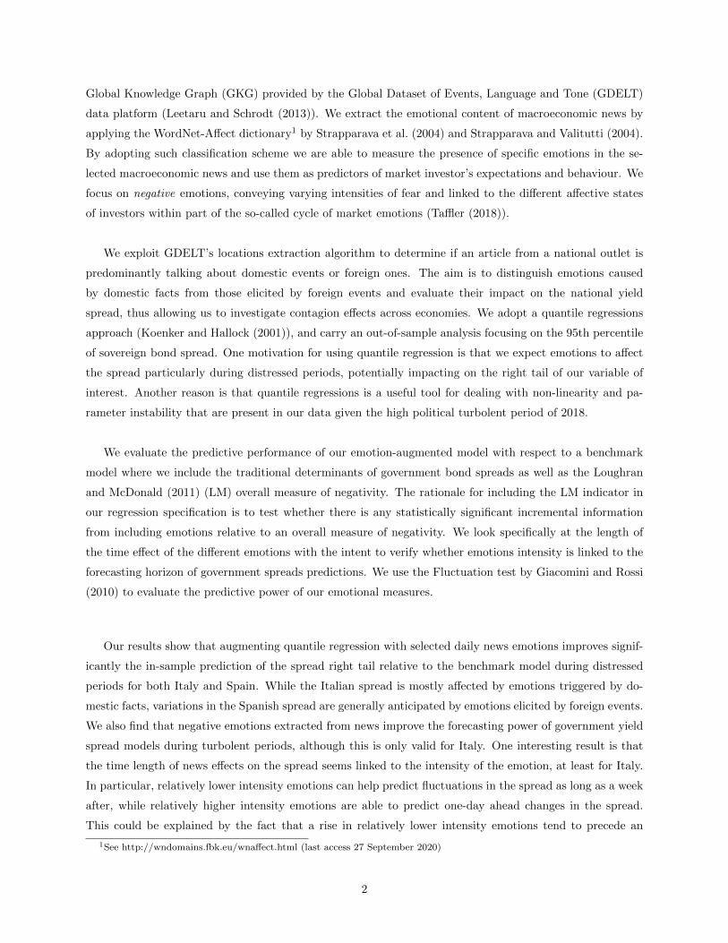
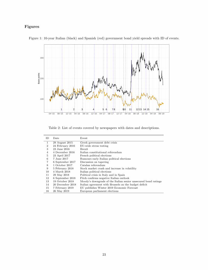
The temporal dynamics of the yield spread for the two countries over the sample period are plotted

in Figure 1, with the vertical dashed lines indicating the timing of some important, stressing, events that

are listed in Table 2. The behaviour of the Italian and Spanish spreads moved closely till late June 2016

when they started diverging in occasion of the Brexit referendum and Spanish elections, when a wave of

uncertainty hit investors, that moved away from the riskier Italian market. At the end of May 2018, a period

of high political turmoil started in both countries. In Spain a motion of no confidence was held against the

prime minister. In Italy the spread sharply rose, passing from around 100 basis points and reaching a peak

of over 250 basis point on the 29th of May 2018, and remained well above 200 basis points afterwards. The

Italian spread lowered in June when the government was formed, but it rose again reaching 350 base points

on the 19th of October, followed by another peak in November when investors started worrying about deficit

spending engagements of the new government and possible conflicts with the European fiscal rules. In the

same period, a wave of anxiety propagated in Europe, causing an increase in borrowing costs especially in

countries from Southern Europe. In 2019, the Italian and the Spanish spreads generally declined, although

some events hit the Italian economy, such as the EU negative economic outlook towards Italy and the Eu-

ropean parliament elections. These facts contributed to a temporary increase of Italian rates in February,

May and August. Although, the Italian interest rates jumped much higher than their Spanish counterparts

6

and risk spillovers seemed to be contained7, Southern European economies appeared to be closely related to

the evolution of the political situation in Italy. The timing of these events are indicated in Figure 1 with

blue vertical dotted lines. The events can be interpreted as stressing events, namely a set of economic and

political events, both domestic and international, that are likely to have triggered a reaction on investors

and hence on the Italian and Spanish spreads.

In our model for forecasting sovereign bond yields spreads, we also include a set of variables that are

traditionally included as determinants of sovereign bond yields spreads, namely credit risk, liquidity risk and

global risk aversion (see Section 2.2). In particular, we use daily returns of FTSEMIB and IBEX for Italy

and Spain, respectively as proxies for credit risk, we measure liquidity risk by taking the bid-ask spread of a

country 10-year government bond yield, and we approximate global risk aversion by the European Implied

volatility index (V STOXX). These variables have been collected from Bloomberg. Summary statistics by

year and by country for these variables are reported in Table 3. We note that, since V STOXX is calculated

at European level, we only report statistics for this variable for Italy as it is identical for Spain. Figures 2-3

show the temporal evolution of spread (expressed in first differences), domestic market returns and liquidity

risk (expressed in first differences) for Italy and Spain, respectively. In Figure 4 we have also plotted the

European investor’s risk aversion (expressed in first differences). It is interesting to observe that in both

countries, credit risk reacts to some of the events listed in Table 2 and having an impact on government

spread across-countries, such as the Greek crisis, the EU stress test, or the Brexit referendum. By building

our news-based indicators we aim at explaining variations in the government yield spread due to national

facts that are not captured by conventional determinants.

3.2 News data

GDELT (Global Database of Events, Language and Tone) is an open, big data platform of meta-information

extracted from broadcast, print, and web news collected at worldwide level and translated nearly in real-

time into English from over 65 different languages (Leetaru and Schrodt (2013)).8 It collects, translates into

English, and processes news worldwide, and updates them on a dedicated web-platform every 15 minutes.9

Three primary data streams are created, one codifying human activities around the world in over 300 cate-

gories, one recording people, places, organizations, millions of themes and thousands of emotions underlying

those events and their interconnection, and one codifying the visual narratives of the world’s news imagery.

Extracted and processed information are stored into different databases, with the most comprehensive among

these being the GDELT Global Knowledge Graph (GKG). GKG is a news-level data set, containing a rich

and diverse array of information. Specifically, for each news GKG extracts information on people, locations

and organizations mentioned in the news, it retrieves counts, quotes, images and themes present in the news

7This phenomenon was also remarked by the president of the European Central Bank, Mario Draghi, during the ECBGovernor Council meeting in Riga in June 15, 2018

8https://www.gdeltproject.org/ (last access 27 September 2020)9See http://data.gdeltproject.org/gdeltv2/lastupdate.txt for the English version, while

http://data.gdeltproject.org/gdeltv2/lastupdate-translation.txt for the translated version (last access 27 September 2020).

7

using a number of popular topical taxonomies, such as the World Bank Topical Taxonomy (WB)10, or the

GDELT built-in topical taxonomy. Finally, it computes a large number of emotional dimensions expressed

by means of commonly used dictionaries, such as the Harvard IV-4 Psycho-social dictionary, the Loughran

and McDonald word list, or the WordNet-Affect dictionary. Specifically, it extracts over 2,200 dimensions,

known as Global Content Analysis Measures (GCAM). The output of such processing is updated on the

GDELT website every fifteen minutes and is freely available to users by means of custom REST APIs. In

terms of volume, GKG analyses over 88 million articles a year and more than 150,000 news outlets. Its

dimension is around 8 TB, growing approximately 2 TB each year. To be able to process the huge amount of

unstructured documents coming from GDELT, we built an ad-hoc Elasticsearch infrastructure (see Gormley

and Tong (2015) for more details). Elasticsearch is a popular and efficient document-store built on the

Apache Lucene11 search library, providing real-time search and analytics for different types of complex data

structures. News data have been downloaded from the GDELT website, re-engineered and stored into our

Elasticsearch platform. This has allowed us to efficiently store and index data in a way that supports fast

search, data retrieval and processing via simple REST APIs.

We have extracted news information from GKG from a set of around 20 newspapers for each of the

examined countries, Italy and Spain, published over the sample period. The chosen newspapers include both

generalist national newspapers with the widest circulation in that country, as well as specialized financial and

economic outlets (Appendix A provides the list of newspapers considered in the analysis). Once collected

the news data, we have mapped these to the relevant trading day. Specifically, we assign to a given trading

day all the articles published during the opening hours of the bond market, namely between 9.00am and

17.30pm. Articles that have been published after the closure of the bond market or overnight are assigned

to the following trading day.12 Following Garcia (2013), we assign the news published during weekends to

Monday trading days, and omit articles published during holidays or in weekends preceding holidays. Once

extracted news information from GKG, we have cleaned the data in various ways. First, to obtain a pool

of news that are not too heterogeneous in length, we have retained only articles that are long at least 100

words.13 Given that we wish to measure emotions related to events concerning bond market investors, rather

then event in general, we have exploited information from the World Bank Topical Taxonomy to understand

the primary focus (theme) of each article and select the relevant news. Such taxonomy is a classification

schema for describing the World Bank’s areas of expertise and knowledge domains representing the language

used by domain experts. Hence, we have selected only articles such that the topics extracted by GDELT fall

into one of the following WB areas of interest: Macroeconomic Vulnerability and Debt, and Macroeconomic

and Structural Policies. In particular, we have retained news that contain in their text at least four keywords

belonging to these themes. The aim is to select news that focus on topics relevant for the bond market,

10https://vocabulary.worldbank.org/taxonomy.html (last access 27 September 2020).11https://lucene.apache.org/ (last access 24 March 2021)12Since the GKG operates on the UTC time, https://blog.gdeltproject.org/new-gkg-2-0-article-metadata-fields/ (last access

27 September 2020), we made a one-hour lag adjustment according to Italian and Spanish time zone.13Such cleaning operation implies dropping only a very small number of articles. For Italy the total number of articles

without the 100 limit on the word count is 9,234 while with such limit is 9,119 (1.26% increment). For Spain we pass from12,209 without the word limit to 12,203 (0.05% increment).

8

while excluding news that only briefly report macroeconomic, debt and structural policies issues.14

A final filter that we applied to our news selection concerns the locations extracted from the text of the

news. Given that we wish to analyze news in a country that predominantly talk about national events, we

have only retained articles for which the main location was, respectively, Italy or Spain. To this end, we

have used the locations information in GKG to infer the main location mentioned in an article. Specifically,

to obtain, for example, all articles that talk about events in Italy, we have only retained those articles that

mention Italy more frequently than all other remaining mentioned countries. The same procedure has been

followed for Spain. After this selection procedure we have obtained a data set of 9,119 articles for Italy, and

12,203 for Spain. In a separate analysis, we have also considered Italian and Spanish articles that mention

Spain and Italy together in the same article, thus having an international focus. This is done with the idea

of capturing domestic emotions triggered by foreign events, possibly due to information contagion effects.

To select such set of articles we have taken all Italian news with main location Italy or Spain or both, and

then all Spanish news with main location Spain or Italy or both. By doing this we have selected a total of

9,458 articles for Italy, and 14,479 for Spain.

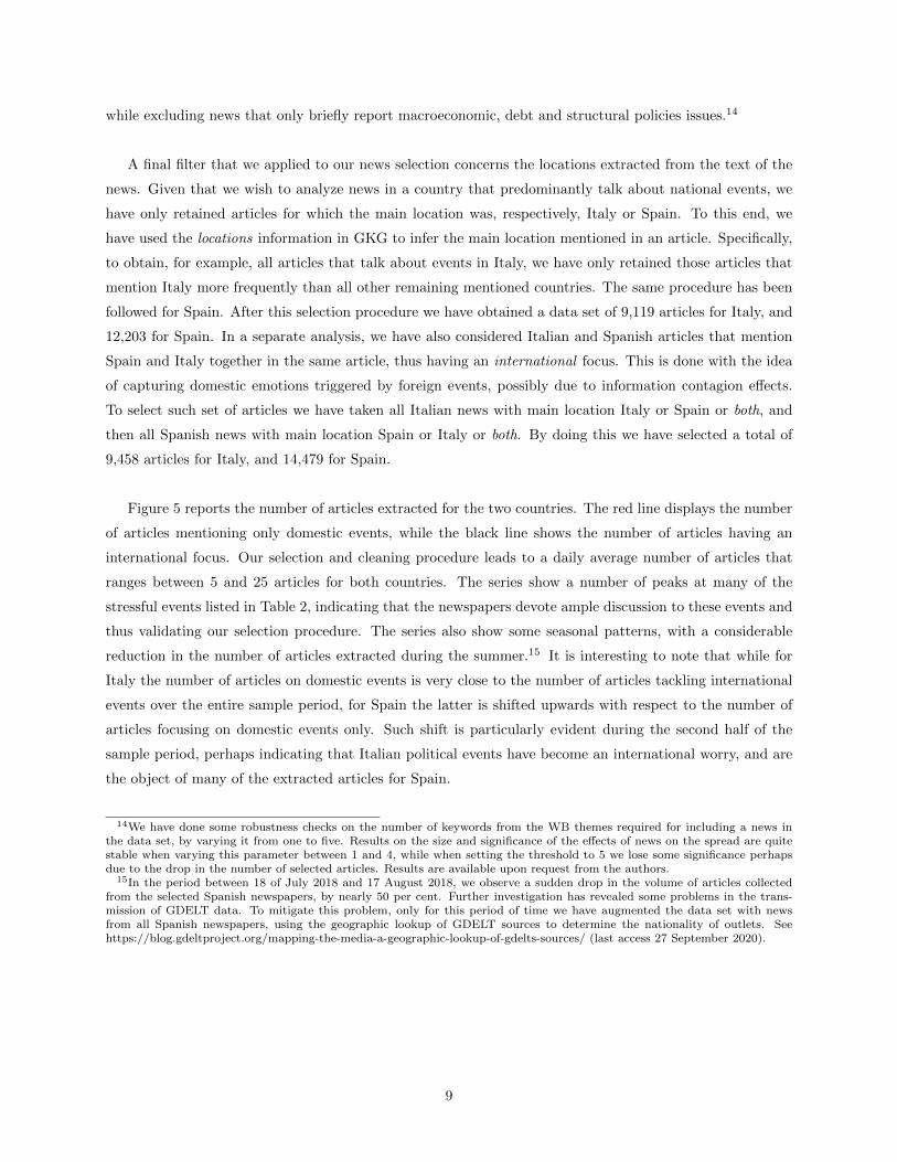
Figure 5 reports the number of articles extracted for the two countries. The red line displays the number

of articles mentioning only domestic events, while the black line shows the number of articles having an

international focus. Our selection and cleaning procedure leads to a daily average number of articles that

ranges between 5 and 25 articles for both countries. The series show a number of peaks at many of the

stressful events listed in Table 2, indicating that the newspapers devote ample discussion to these events and

thus validating our selection procedure. The series also show some seasonal patterns, with a considerable

reduction in the number of articles extracted during the summer.15 It is interesting to note that while for

Italy the number of articles on domestic events is very close to the number of articles tackling international

events over the entire sample period, for Spain the latter is shifted upwards with respect to the number of

articles focusing on domestic events only. Such shift is particularly evident during the second half of the

sample period, perhaps indicating that Italian political events have become an international worry, and are

the object of many of the extracted articles for Spain.

14We have done some robustness checks on the number of keywords from the WB themes required for including a news inthe data set, by varying it from one to five. Results on the size and significance of the effects of news on the spread are quitestable when varying this parameter between 1 and 4, while when setting the threshold to 5 we lose some significance perhapsdue to the drop in the number of selected articles. Results are available upon request from the authors.

15In the period between 18 of July 2018 and 17 August 2018, we observe a sudden drop in the volume of articles collectedfrom the selected Spanish newspapers, by nearly 50 per cent. Further investigation has revealed some problems in the trans-mission of GDELT data. To mitigate this problem, only for this period of time we have augmented the data set with newsfrom all Spanish newspapers, using the geographic lookup of GDELT sources to determine the nationality of outlets. Seehttps://blog.gdeltproject.org/mapping-the-media-a-geographic-lookup-of-gdelts-sources/ (last access 27 September 2020).

9

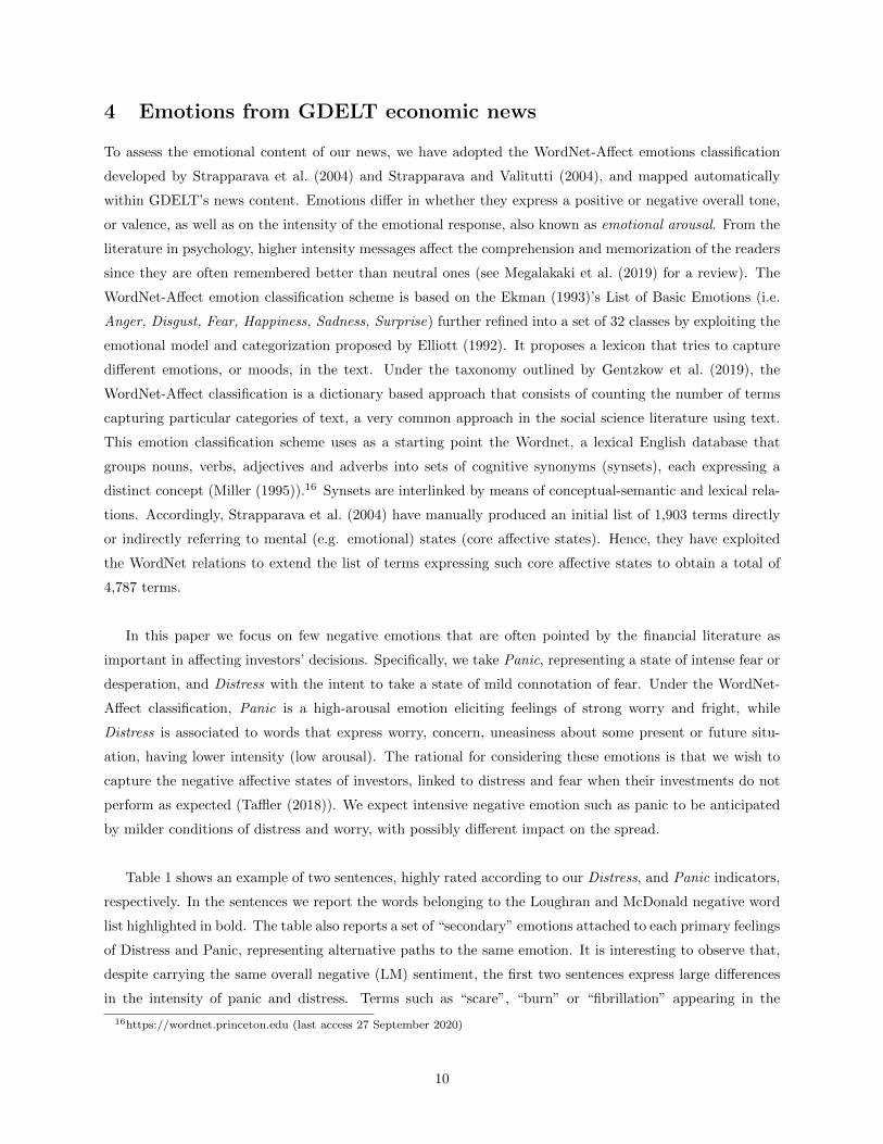
4 Emotions from GDELT economic news

To assess the emotional content of our news, we have adopted the WordNet-Affect emotions classification

developed by Strapparava et al. (2004) and Strapparava and Valitutti (2004), and mapped automatically

within GDELT’s news content. Emotions differ in whether they express a positive or negative overall tone,

or valence, as well as on the intensity of the emotional response, also known as emotional arousal. From the

literature in psychology, higher intensity messages affect the comprehension and memorization of the readers

since they are often remembered better than neutral ones (see Megalakaki et al. (2019) for a review). The

WordNet-Affect emotion classification scheme is based on the Ekman (1993)’s List of Basic Emotions (i.e.

Anger, Disgust, Fear, Happiness, Sadness, Surprise) further refined into a set of 32 classes by exploiting the

emotional model and categorization proposed by Elliott (1992). It proposes a lexicon that tries to capture

different emotions, or moods, in the text. Under the taxonomy outlined by Gentzkow et al. (2019), the

WordNet-Affect classification is a dictionary based approach that consists of counting the number of terms

capturing particular categories of text, a very common approach in the social science literature using text.

This emotion classification scheme uses as a starting point the Wordnet, a lexical English database that

groups nouns, verbs, adjectives and adverbs into sets of cognitive synonyms (synsets), each expressing a

distinct concept (Miller (1995)).16 Synsets are interlinked by means of conceptual-semantic and lexical rela-

tions. Accordingly, Strapparava et al. (2004) have manually produced an initial list of 1,903 terms directly

or indirectly referring to mental (e.g. emotional) states (core affective states). Hence, they have exploited

the WordNet relations to extend the list of terms expressing such core affective states to obtain a total of

4,787 terms.

In this paper we focus on few negative emotions that are often pointed by the financial literature as

important in affecting investors’ decisions. Specifically, we take Panic, representing a state of intense fear or

desperation, and Distress with the intent to take a state of mild connotation of fear. Under the WordNet-

Affect classification, Panic is a high-arousal emotion eliciting feelings of strong worry and fright, while

Distress is associated to words that express worry, concern, uneasiness about some present or future situ-

ation, having lower intensity (low arousal). The rational for considering these emotions is that we wish to

capture the negative affective states of investors, linked to distress and fear when their investments do not

perform as expected (Taffler (2018)). We expect intensive negative emotion such as panic to be anticipated

by milder conditions of distress and worry, with possibly different impact on the spread.

Table 1 shows an example of two sentences, highly rated according to our Distress, and Panic indicators,

respectively. In the sentences we report the words belonging to the Loughran and McDonald negative word

list highlighted in bold. The table also reports a set of “secondary” emotions attached to each primary feelings

of Distress and Panic, representing alternative paths to the same emotion. It is interesting to observe that,

despite carrying the same overall negative (LM) sentiment, the first two sentences express large differences

in the intensity of panic and distress. Terms such as “scare”, “burn” or “fibrillation” appearing in the

16https://wordnet.princeton.edu (last access 27 September 2020)

10

second sentence are much more emotionally arousing than milder expressions like “concern”, “risky” present

in the first sentence. One possibility to capture such different intensity in negativity of news would be to

adopt a graded system that measures how negative/positive a specific term is. However, the calculation of

an average, daily, tonality could weep out the effect of specific segments of the polarity. On the contrary,

measuring the emotional content of news, can help disentangle the contribution of specific components of

the polarity to the total forecasting ability.

Table 1: Example of sentences conveying emotions of Distress and Panic

Primary SecondaryEmotion Emotion Example

Distress Apprehension, Worry, The signals expressed by the financial markets are beginningUneasiness, Concern to be a source of concern and certainlyNegative suspense reflect a fundamental medium-long term risky situation.

Panic Fright, The final bill scares the investors: burnedShock, Scare, 12 billion euros in one dayTerror, Horror, since the fibrillation began forHysteria the political situation.

Notes: The first sentence is taken form https://www.investireoggi.it/obbligazioni/politica-monetaria-e-incertezza-politica-in-italia/, while the second from http://www.ilgiornale.it/news/politica/voto-fa-paura-spread-235-borsa-brucia-tutto-2018-1533515.html.

For each day in the sample, we calculate the total number of words that carry the negative emotions

Distress and Panic appearing in the selected articles published on that day. We standardize these variables

by dividing their values by the total number of words in a given day. We then calculate moving averages

with a rolling window of 5 open-market days, with the intent to incorporate in our regression model news

information referring to the last week. A number of studies also include information on the sentiment for

the previous 5 days in their regression (see, for example, Liu (2014), or Tetlock (2007) and Garcia (2013)).

In particular, for a specific country, we set:

Emotiont =

t∑s=t−4

1

5

WCemotion,s

WCs, (1)

where WCemotion,s is the words count of the specific emotion for selected articles published in the country

at time s according to the Wordnet-Affect lexicon, and WCs is the total words count of all articles published

in the day.17 To facilitate interpretation of regression coefficients, we rescale our indicator to have unit

variance.

We next move to our emotion-augmented statistical model for government yield spreads.

17We have done some robustness checks and run several regressions by varying the smoothing parameter in equation (1)between 3 and 20. Results are similar to those reported in the paper and are available upon request.

11

5 Methods

The main objective of the analysis is to assess how negative emotions impact on the yield spreads during

stressed periods.

Following Bernal et al. (2016), we assume that the qth percentile of sovereign bond spread expressed in

first differences represents a situation of financial distress. Accordingly, let ∆Spreadqt+h be the qth percentile

of sovereign bond spread for a given country expressed in first differences. We adopt a quantile regression

approach and consider the following emotion-augmented quantile regression (Koenker and Bassett (1978)):

∆Spreadt+1 = αq + δq0∆Spreadt + δq1Xt + γqLMt−h + βqEmotiont−h + εt+1 (2)

where Xt includes the variables that are traditionally included in models for government bond spreads to

control for various sources of risk, namely credit risk, liquidity risk and risk aversion. LMt is the LM negative

indicator expressed as the fraction of the words belonging to the LM negative word list present in the text of

the selected articles, and Emotiont is our emotion variable, as defined in (1). We note that we have included

the variable ∆Spreadt amongst the regressors to account for the state of the market.18 Further, in our

regression we also control for LM with the aim to test whether including our emotion indicators provide any

statistically significant incremental information to such general measure of negativity. In Equation (2), h is

the length of time needed for our news variables to take effect on the dependent variable. In our empirical

exercise we try different time horizons, varying from 1 day (h = 1) up to 1 week lag (h = 5) for the news

to impact on the dynamics of the spread. As for the choice of the quantile level, q, following Bernal et al.

(2016), we focus on the right tail of sovereign bond spread expressed in first differences, and set q = 0.95.

In fact, this measure represents a situation of financial distress where we believe news are most important

in anticipating variations in the spread. However, in Section 6 we also carry a small exploratory analysis to

evaluate how the size and significance of estimated regression coefficients attached to the emotion indicators

in equation 2 vary across quantiles.

We estimate and evaluate the performance of Model (2) against the benchmark model containing only

financial variables and LM indicator (i.e., where we set βq = 0) in an in-sample and an out-of-sample exercise.

In the in-sample analysis, we calculate the R2 following the procedure outlined by Koenker and Machado

(1999). Finally, we compute confidence intervals for the estimated coefficients by using the Koenker (1994)

approach based on inversion of a rank test.

To evaluate the forecasting performance of Model (2) against that of the benchmark model, we split the

sample into two sub-samples of similar size: we take T0 = 569 observations for estimation for h = 1 (567

for h = 5) and use the remaining observations for testing. Specifically, for each time horizon h, and for

18We have also tried a specification where we have included the variable Spreadt rather than ∆Spreadt amongst the regressors.The main results are similar to those reported in the paper, and hence we have decided not to show them, but are availableupon request.

12

t = T0 + 1, T0 + 2, ..., T the forecast errors using information up to time t are:

εemotiont+1 = ρq(∆Spreadt+1 − ∆Spreadt+1,emotion) (3)

εbenchmarkt+1 = ρq(∆Spreadt+1 − ∆Spreadt+1,benchmark) (4)

where ρq is the so-called check function, given by ρq(z) = (q− I(z < 0))z, ∆Spreadt+1,emotion is the forecast

of the spread using the emotion-augmented quantile regression (2), and ∆Spreadt+1,benchmark is the forecast

of the spread using the benchmark model.

Our sample covers a period of high political turmoil, as also evident from Figure 1 and Table 3. The

large variations in the yield spreads occurring particularly during the second half of the sample period hide

important changes in the impact of our regressors on the spread over time, and undermine the validity of

standard forecasting tests. As also pointed by Giacomini and Rossi (2010), in the presence of structural

instability, the relative performance of the two models may itself be time-varying, and thus averaging this

evolution over time will result in a loss of information. By selecting the model that performed best on average

over a particular historical sample, one may ignore the fact that the competing model produced more accurate

forecasts when considering only the recent past. To account for this time variability, in this paper we carry

a rolling-windows analysis. Specifically, we re-estimate the unknown parameters in Equation (2) at each

t = T0 + h, T0 + h+ 1, ..., T over a rolling window of T0 days including data indexed t− h− T0 + 1, ..., t− h,

where we set T0 = 569 observations for estimation for h = 1 (567 for h = 5). For each rolling window,

we plot the estimated coefficients, confidence intervals and R2 against time. For evaluating the forecasting

performance of our models, we adopt the Fluctuation test proposed by Giacomini and Rossi (2010) in order

to assess over time, the ability of our news-based emotional indicators to track and anticipate the emotional

state of markets over classical predictors during periods of turmoil. The Fluctuation test statistics consists

of calculating the Diebold and Mariano (1995) (DM) test statistics statistic over a rolling out-of sample

window of size m. When computing this test, we set the ratio between the rolling window length and the

out-of-sample length, µ = m/(T − T0), equal to 0.30, as in Giacomini and Rossi (2010), and use the HAC

estimator for the long-run variance. Finally, in selecting the relevant critical values for the Fluctuation test

we consider a two-sided test and assume a nominal size of 5 per cent (see Table I in Giacomini and Rossi

(2010)).

13

6 Empirical results

6.1 Dynamics of emotions

Figure 6 displays the time series of our emotion variables for Italy (top) and Spain (bottom). The dashed

lines in these graphs indicate our emotion indicators calculated on articles that speak about both domestic

and international events. Articles extracted carry a daily average of 3 to 18 words conveying Distress and

2 to 8 words carrying Panic, hence, articles contain on average relatively more Distress than Panic. This

result could be explained by the fact that milder emotions, are likely to appear more frequently relative to

high arousal emotions, such as Panic, that are only elicited in extremely stressing situations. The graph

shows important time variation in Distress and Panic variables for both Italy and Spain, with the two vari-

ables spiking at many of the stressing events listed in Table 2. Specifically, we observe peaks in the Italian

emotions series during the Greece debt crisis in August 201519, the Italian constitutional referendum in

December 2016 and Italian political elections in March 2018, as well during the period of political turmoil

from May to October 2018. Over these months we not only observe spikes but also a rising trend in our

emotional variables, indicating an overall increase in negativity. As for Spain, the emotion indicators peak

during the Spanish general elections (and Brexit Referendum) in June 2016, in occurrence of the October

2017 Catalan referendum, and during the Spanish political crisis in May 2018.

Looking at the evolution of the dashed lines in the bottom graph, it is interesting to observe that,

during the period of Italian political turmoil and successively, when Italy was discussing deficit spending

engagements with the European Union, emotions from Spanish articles speaking about international events

considerably diverge from those that focus on domestic facts alone. One explanation for this result is that

negative emotions in Spanish national news are mainly triggered by Italian political events. If we compare the

peaks in Distress with those in Panic, we also observe that both series move upwards almost simultaneously,

although Distress tends to rise faster than Panic, and Panic seems to revert back to zero more speedily than

Distress. This evidence is in line with the financial emotional cycle, where mild worry turns into stronger

feelings of fear. Figure 7 shows the temporal evolution of the LM indicator. It is interesting to observe

that the behaviour of the LM follows a pattern that is similar to that of our emotional variables, rising in

correspondence of the majority of the stressing events previously identified. Another interesting features

that emerges from these graphs is that there are on average more negative words in Spanish news stories

when international events are taken into account, suggesting attention bias towards what happens abroad.

19Although in our articles considers predominantly Italian events, the Greece debt crisis emerges as an important issue inthis period.

14

6.2 Regression analysis

Figure 8 displays the size and significance of the estimated coefficients attached to our news indicators Panic

and Distress in (1) when varying the parameter q between 0.05 and 0.95 at intervals of 0.05. It is interesting

to observe that the news indicators are significantly different from zero for q that lies either near zero or

near 1, while they are not significant for quantiles around 0.5. This result seems to indicate that news are

most important in anticipating variations in the spreads particularly during period of high uncertainty and

distress, and support the choice of q = 0.95 in the estimation of equation (1). Accordingly, the rest of the

analysis focuses in the case q = 0.95. We now turn to the rolling-window regression analysis.

Figure 9 visualises the evolution over the rolling windows of the estimated coefficients from Equation (2)

and associated confidence intervals. It shows results for Italy and Spain when setting h = 0, 1, 5 and the

news focus on domestic events, while Figure 10 show the same graphs when the focus is on domestic and

international events.20 The rolling-window estimation uncovers important time variations both in the size

and significance of coefficients. For Italy, we observe that starting from the beginning of the political crisis

in May 2018, all estimated coefficients turn strongly significant for all values of h until the end of the sample.

Over this period of time, the estimated coefficients attached to our emotion variables are always positive.

Specifically, one standard deviation shock to the Distress variable produces a change in the spread that range

between 2.5 and 6 basis points, while such change ranges between 2.5 and 5 basis points for a shock of the

same amplitude on the Panic indicator. For all indicators, the coefficients tend to rise when using larger

values of h, although the associated confidence bands also tend to widen. Similar results are obtained when

extending the focus to international events, indicating that the predictive performance of the Italian news is

mainly driven by concern and scare triggered by domestic events. This result is somewhat expected, given

that for Italy, as evident from Figure 6, our news indicators are almost identical when focusing on domestic

or international events.

Moving to Spain, Figure 9 shows that when focusing on domestic news, only the coefficients attached

to Panic, for h = 0 (and to some extend for h = 1) are statistically significant. However, it is interesting

to observe from Figure 10 that when expanding the focus to international events, Panic and Distress turn

strongly significant in May 2018. This result seems to support the view that for Spain, the power of news

in predicting variations in government spread is mostly explained by emotions triggered by international

rather than domestic events. The effects of one standard deviation shock to our emotion variables produces

a change on the Spanish spread that range between 1 and 2 basis points with values that can reach 3 basis

points for Panic at short time horizons. While the statistical significance of parameters attached to Panic

is maintained till the end of the sample, for Distress it is mainly concentrated in the second part of 2018.

We also notice a deterioration of the forecasting performance at longer horizons. While for h = 0, 1 the

parameters attached to Panic are strongly significant over a long interval of time, it turns insignificant for

h = 5. We also observe that the values of the estimated coefficients are overall smaller relative to the Italian

20For ease of exposition, results for the case h = 2, 3, 4 are not reported but are available upon request.

15

case.

Figures 11 and 12 plots the difference in adjusted R2 between the models with our news indicators and

the benchmark over the rolling windows. For ease of exposition, in the rest of the paper we only report the

case of domestic news for Italy and the case of domestic and international news for Spain. In correspondence

of the Italian political crisis in May 2018, the in-sample performance of the model improves. In particular,

while Distress seems to boost the in-sample performance at longer forecasting horizons (i.e., h = 5), Panic is

more important in explaining contemporaneous reactions of Italian spread (i.e., for h = 0). Hence, according

to our results, milder emotions seem to capture the stressed state of the market with predictive power at

longer time horizons, as opposed to stronger emotions that have important instantaneous effects. This re-

sult supports the view that milder emotions trigger stronger ones that are then associated to instantaneous

variations in the spread. For Spain, Panic is the emotion that mostly contributes to the in-sample fitting

performance for h = 0, 1, while Distress is more important at h = 5, although the rolling R2 quickly reduces

after the peak in the May 2018. Clearly, the Spanish spread is driven by strong emotions triggered by

international events.

We now turn to the results of the Giacomini and Rossi (2010) Fluctuation test, reported in Figures

13 and 14 for h = 1, 5. This test, by calculating the DM test over a rolling out-of sample window of a

pre-specified size is more reliable than the simple DM statistics calculated by pooling observations from

the full sample. The graphs show strong empirical evidence of time variation in the relative performance

of the news-augmented models relative to the benchmark model that includes only financial variables. For

Italy, and when setting h = 1, the Fluctuation test for our emotion variables turns significant relative to

the benchmark soon after at the start of the political crisis, with Panic turning significant on the 5th of

June, followed by Distress on the 8th of June. For Panic we observe an increase in the significance of the

test starting from late October 2018, when Moody’s downgraded the Italian senior unsecured bond rating,

until the end of January 2019. As for Distress, it remains significant until mid-August 2018. In the case

of the 5-steps ahead forecasts, only Distress falls below the critical value line, over the period starting in

mid-August and ending in November 2018 with the exception of a few days at the beginning of October. We

observe that this is a period of persistent concern for market participants given the negative outlook for the

Italian economy provided by Fitch in September 2018 and the tension between Italy and the European Union

concerning the Italian financial and economic budget plan later that year. Overall, these graphs confirm the

better forecasting ability of Panic at a short time horizon (h = 1) and of Distress at a longer time horizon

(h = 5). As for Spain, our emotions do not provide statistically significance neither at long nor at short

time horizon. While distress and panic triggered by international events contribute to the in-sample fitting

performance of our model for Spain, the predictive power of our emotions vanishes in the out-of-sample

exercise.

16

7 Conclusions

In this paper we studied the effect of news emotions to help predicting changes in government yield bond

spread in Italy and Spain. Empirical results suggested that augmenting quantile regression with selected

daily news emotions significantly improve the predictive power of conventional models for government yield

bond spread, for both Italy and Spain, also after controlling for the overall negativity in the news text

measured by the Loughran and McDonald (2011) dictionary. One interesting finding is that the focus of

news seems to play an important role in explaining variations in the government yield spreads, with Italy

mostly worried about the domestic economic situation, and Spanish anxiety mostly triggered by interna-

tional events. When using our news-based indicators for forecasting future variations of government yield

bond spreads, our emotion variables showed some forecasting ability only for Italy. In particular, for this

country the relatively lower intensity emotion of Distress was able to forecast fluctuations in the spread as

long as a week after, while the relatively higher intensity emotion of Panic improved forecasts of one day

ahead changes in the spread.

Overall, the analysis of emotions extracted from news seems a promising area of research, particularly

useful for capturing future intentions of agents in financial markets. One interesting extension of this work

is to consider a wider set of emotions, both positive and negative, and use them to forecast both tails of

the distribution of government yield spreads. Future work could also consider adopting machine learning

techniques to look at additional features of articles and their non-linear effect on the dependent variable.

This will be the object of a future study.

17

Acknowledgments

The authors would like to thank the colleagues of the Centre for Advanced Studies at the Joint Research

Centre of the European Commission for helpful guidance and support during the development of this re-

search work.

We would like to thank Sebastiano Manzan, Luca Barbaglia, Javier J. Perez, Barbara Rossi, Fabio Trojani,

Leonardo Iania, Laurent Callot, Guillaume Chavillon as well as the participants at the JRC Workshop on

Big Data and Economic Forecasting 2019, New Techniques and Technologies for Official Statistics 2019, the

Smart Statistics for Smart Application Conference of the Italian Statistical Society in Milan, Mining Data

for Financial Application Workshop in Wurzburg, CFE 2019 Conference in London for helpful comments

and remarks.

18

References

Ackert, L., Bryan, C., Deaves, R., 2003. Emotion and financial markets. Economic Review 88, 33–41.

Afonso, A., Arghyrou, M. G., Kontonikas, A., 2015. The determinants of sovereign bond yield spreads in the

EMU. ECB Working Paper 1781.

Afonso, A., Furceri, D., Gomes, P., 2012. Sovereign credit ratings and financial markets linkages: Application

to european data. Journal of International Money and Finance 31, 606 – 638.

Allee, K. D., DeAngelis, M. D., 2015. The structure of voluntary disclosure narratives: Evidence from tone

dispersion. Journal of Accounting Research 53 (2), 241–274.

Apergis, N., 2015. Forecasting credit default swaps (cdss) spreads with newswire messages: Evidence from

european countries under financial distress. Economics Letters 136, 92 – 94.

Apergis, N., Lau, M. C. K., Yarovaya, L., 2016. Media sentiment and CDS spread spillovers: Evidence from

the GIIPS countries. International Review of Financial Analysis 47 (C), 50–59.

Attinasi, M.-G., Checherita, C., Nickel, C., 2009. What explains the surge in euro area sovereign spreads

during the financial crisis of 2007-09? ECB Working Paper 1131.

Baber, A., Brandt, M. W., Kavajecz, K. A., 2009. Flight-to-quality or flight-to-liquidity? Evidence from the

Euro-area bond market. The Review of Financial Studies 22 (3), 925–957.

Baker, S. R., Bloom, N., Davis, S. J., 2016. Measuring economic policy uncertainty. Quarterly Journal of

Economics 131 (4), 1593–1636.

Barbaglia, L., Consoli, S., Manzan, S., 2020. Monitoring the business cycle with fine-grained, aspect-based

sentiment extraction from news. Lecture Notes in Computer Science (including subseries Lecture Notes in

Artificial Intelligence and Lecture Notes in Bioinformatics) 11985 LNAI, 101–106.

Beetsma, R., Giuliodori, M., de Jong, F., Widijanto, D., 2013. Spread the news: The impact of news on

the European sovereign bond markets during the crisis. Journal of International Money and Finance 34,

83–101.

Bernal, O., Gnabo, J.-Y., Guilmin, G., 2016. Economic policy uncertainty and risk spillover in the Eurozone.

Journal of International Money and Finance 65 (C), 24–45.

Blommestein, H., Eijffinger, S., Qian, Z., 08 2012. Animal Spirits in the Euro Area Sovereign CDS Market.

CEPR Discussion Paper.

Chen, J., Jiang, F., Tong, G., 2017. Economic policy uncertainty in China and stock market expected returns.

Accounting & Finance 57 (5), 1265–1286.

Codogno, L., Favero, C., Missale, A., 2003. Yield spreads on EMU government bonds. Economic Policy

18 (37), 503–532.

19

De Santis, R. A., 2012. The Euro area sovereign debt crisis: Safe haven, credit rating agencies and the spread

of the fever from Greece, Ireland and Portugal. Tech. rep., ECB Working Papers.

Diebold, F. X., Mariano, R. S., 1995. Comparing predictive accuracy. Journal of Business & Economic

Statistics 13 (3), 253–263.

Dridi, A., Atzeni, M., Reforgiato Recupero, D., 2018. FineNews: Fine-grained semantic sentiment analysis

on financial microblogs and news. International Journal of Machine Learning and Cybernetics, 1–9.

Ekman, P., 1993. Facial expression and emotion. American Psychologist 48 (4), 384–392.

Elliott, C., 1992. The affective reasoner: A process model of emotions in a multi-agent system. Tech. Rep. 32,

The Institute for the Learning Sciences, PhD Thesis, Northwestern University.

Favero, C., 2013. Modelling and forecasting government bond spreads in the Euro area: A GVAR model.

Journal of Econometrics 177 (2), 343–356.

Fenton-O’Creevy, M., Soane, E., Nicholson, N., Willman, P., 2011. Thinking, feeling and deciding: The influ-

ence of emotions on the decision making and performance of traders. Journal of Organizational Behavior

32 (8), 1044–1061.

Gade, T., Salines, M., Glockler, G., Strodthoff, S., 2013. Loose lips sinking markets? The impact of political

communication of on sovereign bond spreads. Tech. rep., ECB Occasional Paper Series n. 150.

Garcia, D., 2013. Sentiment during recessions. The Journal of Finance 68 (3), 1267–1300.

Gentzkow, M., Kelly, B., Taddy, M., 2019. Text as data. Journal of Economic Literature 57 (3), 535–574.

Giacomini, R., Rossi, B., 2010. Forecast comparisons in unstable environments. Journal of Applied Econo-

metrics 25 (4), 595–620.

Goetzmann, W., Kim, D., Shiller, R., 2016. Crash beliefs from investor surveys. NBER Working Papers

22143, National Bureau of Economic Research, Inc.

Gormley, C., Tong, Z., 2015. Elasticsearch: The definitive guide. O’Reilly, Media.

Griffith, J., Najand, M., Shen, J., 2020. Emotions in the stock market. Journal of Behavioral Finance 21 (1),

42–56.

Kliponen, J., Laakkonen, H., Vilmunen, J., 2015. Sovreign risk, european crisis-resoultion policies and bond

yields. International Journal of Central Banking 11, 285–323.

Koenker, R., 1994. Confidence intervals for regression quantiles. In: Mandl, P., Huskova, M. (Eds.), Asymp-

totic Statistics. Physica-Verlag HD, Heidelberg, pp. 349–359.

Koenker, R., Bassett, G., 1978. Regression quantiles. Econometrica 46 (1), 33–50.

Koenker, R., Hallock, K., 2001. Quantile regression. Journal of Economic Perspectives 15, 143–156.

20

Koenker, R., Machado, J. A. F., 1999. Goodness of fit and related inference processes for quantile regression.

Journal of the American Statistical Association 94 (448), 1296–1310.

Leetaru, K., Schrodt, P. A., 2013. GDELT: global data on events, location and tone, 1979-2012. Tech. rep.,

KOF Working Papers.

Liu, S., 2014. The impact of textual sentiment on sovereign bond yield spreads: Evidence from the Eurozone

crisis. Multinational Finance Journal 18 (3/4), 215–248.

Loughran, T., McDonald, B., 2011. When is a liability not a liability? Textual analysis, dictionaries and

10-ks. Journal of Finance 66 (1), 35–65.

Mayew, W. J., Venkatachalam, M., 2012. The power of voice: Managerial affective states and future firm

performance. The Journal of Finance 67 (1), 1–43.

Megalakaki, O., Ballenghein, U., Baccino, T., 2019. Effects of valence and emotional intensity on the com-

prehension and memorization of texts. Frontiers in Psychology 10, 179.

Miller, G. A., Nov. 1995. Wordnet: A lexical database for english. Commun. ACM 38 (11), 39–41.

Mohl, P., Sondermann, D., 2013. Has political communication during the crisis impacted sovereign bond

spreads in the Euro area? Applied Economics Letters 20 (1), 48–61.

Oliveira, L., Curto, J. D., Pedro, N. J., 2012. The determinants of sovereign credit spread changes in the

Euro-area zone. Journal of International Financial Markets, Institutions and Money 22 (2), 278–304.

Reforgiato Recupero, D., Presutti, V., Consoli, S., Gangemi, A., Nuzzolese, A., 2015. Sentilo: Frame-based

sentiment analysis. Cognitive Computation 7 (2), 211–225.

Schwarz, K., 2019. Mind the gap: Disentangling credit and liquidity in risk spreads. Review of Finance

23 (3), 557–597.

Shapiro, A. H., Sudhof, M., Wilson, D., 2018. Measuring news sentiment. Federal Reserve Bank of San

Francisco Working Paper.

Shiller, R. J., 2003. From efficient markets theory to behavioral finance. The Journal of Economic Perspectives

17 (1), 83–104.

Strapparava, C., Valitutti, A., 2004. WordNet-Affect: An affective extension of WordNet. Proceedings of the

4th International Conference on Language Resources and Evaluation (LREC 2004), 1083–1086.

Strapparava, C., Valitutti, A., Stock, O., 2004. Developing affective lexical resources. PsychNology Journal.

Taffler, R., 2018. Emotional finance: Investment and the unconscious. The European Journal of Finance

24 (7-8), 630–653.

Tetlock, P. C., 2007. Giving content to investor sentiment: The role of media in the stock market. Journal

of Finance 62 (3), 1139–1168.

21

Tetlock, P. C., Saar-Tsechansky, M., Macskassy, S., 2008. More than words: Quantify language to measure

firms’ fundamentals. Journal of Finance 63 (3), 1437–1467.

Thorsrud, L. A., 2016. Nowcasting using news topics. Big Data versus Big Bank. Norges Bank Working

Paper.

Thorsrud, L. A., 2018. Words are the new numbers: A news coincident index of the business cycle. Journal

of Business & Economic Statistics, 1–17.

Yuan, H., Lau, R. Y. K., Wong, M. C., Li, C., 2018. Mining emotions of the public from social media

for enhancing corporate credit rating. In: Proceedings - 2018 IEEE 15th International Conference on

e-Business Engineering, ICEBE 2018. No. 8592626. pp. 25–30.

22

Figures

Figure 1: 10-year Italian (black) and Spanish (red) government bond yield spreads with ID of events.

1 2 3 4 5 6 7 8 910 11 12 13 14 15 16

100

200

300

04−15 08−15 12−15 04−16 08−16 12−16 04−17 08−17 12−17 04−18 08−18 12−18 04−19 08−19

Bas

is p

oint

s

Table 2: List of events covered by newspapers with dates and descriptions.

ID Date Event

1 29 August 2015 Greek government debt crisis2 24 February 2016 EU-wide stress testing3 23 June 2016 Brexit4 4 December 2016 Italian constitutional referendum5 23 April 2017 French political elections6 7 June 2017 Rumours early Italian political elections7 6 September 2017 Discussion on tapering8 1 October 2017 Catalan referendum9 5 February 2018 Stock market crash and increase in volatility10 4 March 2018 Italian political elections11 29 May 2018 Political crisis in Italy and in Spain12 6 September 2018 Fitch confirms negative Italian outlook13 19 October 2018 Moody’s downgrade of the Italian senior unsecured bond ratings14 20 December 2018 Italian agreement with Brussels on the budget deficit15 7 February 2019 EU publishes Winter 2019 Economic Forecast16 26 May 2019 European parliament elections

23

Figure 2: Government yield spread (in first differences), credit risk (market’s returns), liquidity risk (in firstdifferences) for Italy.

−20

0

20

04−15 08−15 12−15 04−16 08−16 12−16 04−17 08−17 12−17 04−18 08−18 12−18 04−19 08−19

∆spread Italy

−10

−5

0

04−15 08−15 12−15 04−16 08−16 12−16 04−17 08−17 12−17 04−18 08−18 12−18 04−19 08−19

CRD (FTSEMIB index)

−2

−1

0

1

2

3

04−15 08−15 12−15 04−16 08−16 12−16 04−17 08−17 12−17 04−18 08−18 12−18 04−19 08−19

∆Liq Italy

24

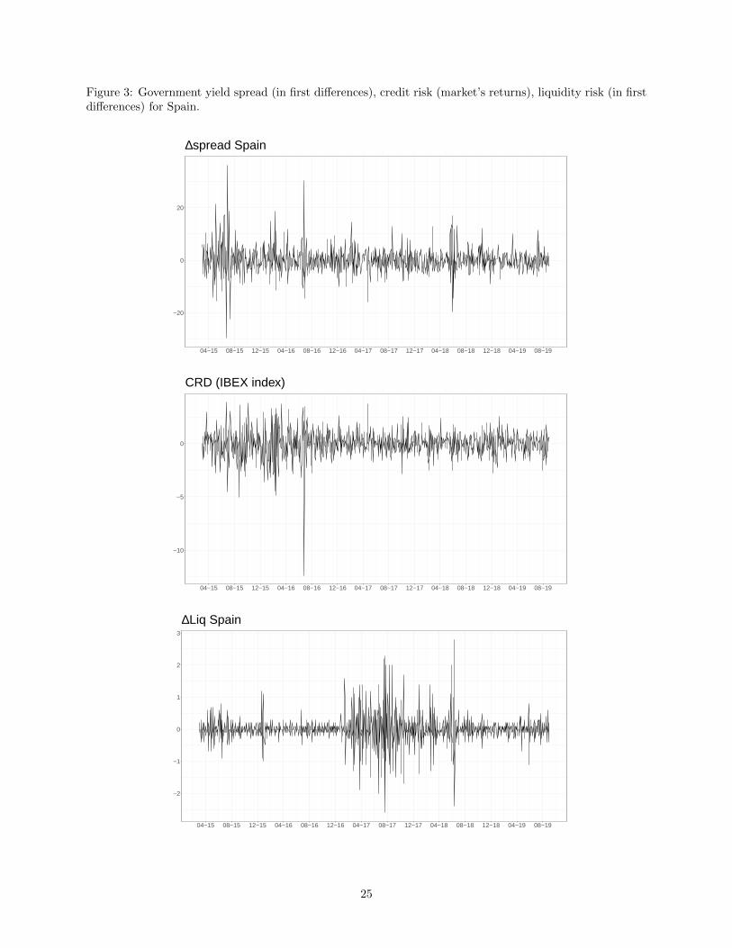
Figure 3: Government yield spread (in first differences), credit risk (market’s returns), liquidity risk (in firstdifferences) for Spain.

−20

0

20

04−15 08−15 12−15 04−16 08−16 12−16 04−17 08−17 12−17 04−18 08−18 12−18 04−19 08−19

∆spread Spain

−10

−5

0

04−15 08−15 12−15 04−16 08−16 12−16 04−17 08−17 12−17 04−18 08−18 12−18 04−19 08−19

CRD (IBEX index)

−2

−1

0

1

2

3

04−15 08−15 12−15 04−16 08−16 12−16 04−17 08−17 12−17 04−18 08−18 12−18 04−19 08−19

∆Liq Spain

25

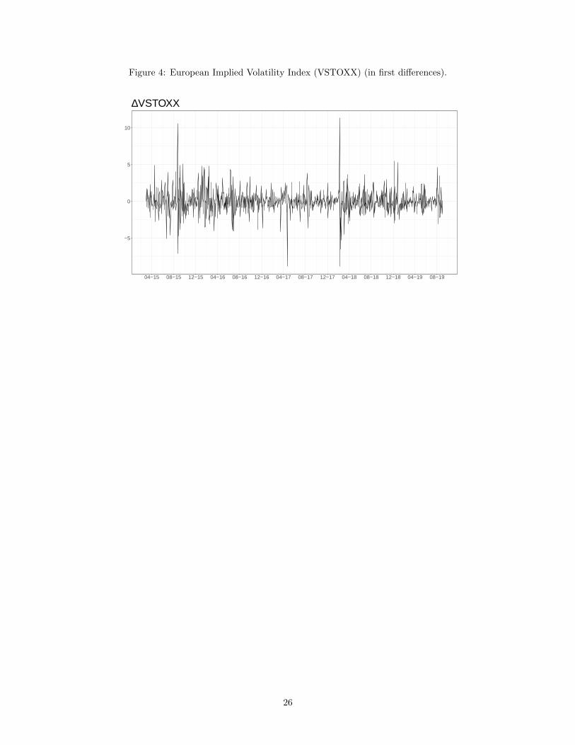
Figure 4: European Implied Volatility Index (VSTOXX) (in first differences).

−5

0

5

10

04−15 08−15 12−15 04−16 08−16 12−16 04−17 08−17 12−17 04−18 08−18 12−18 04−19 08−19

∆VSTOXX

26

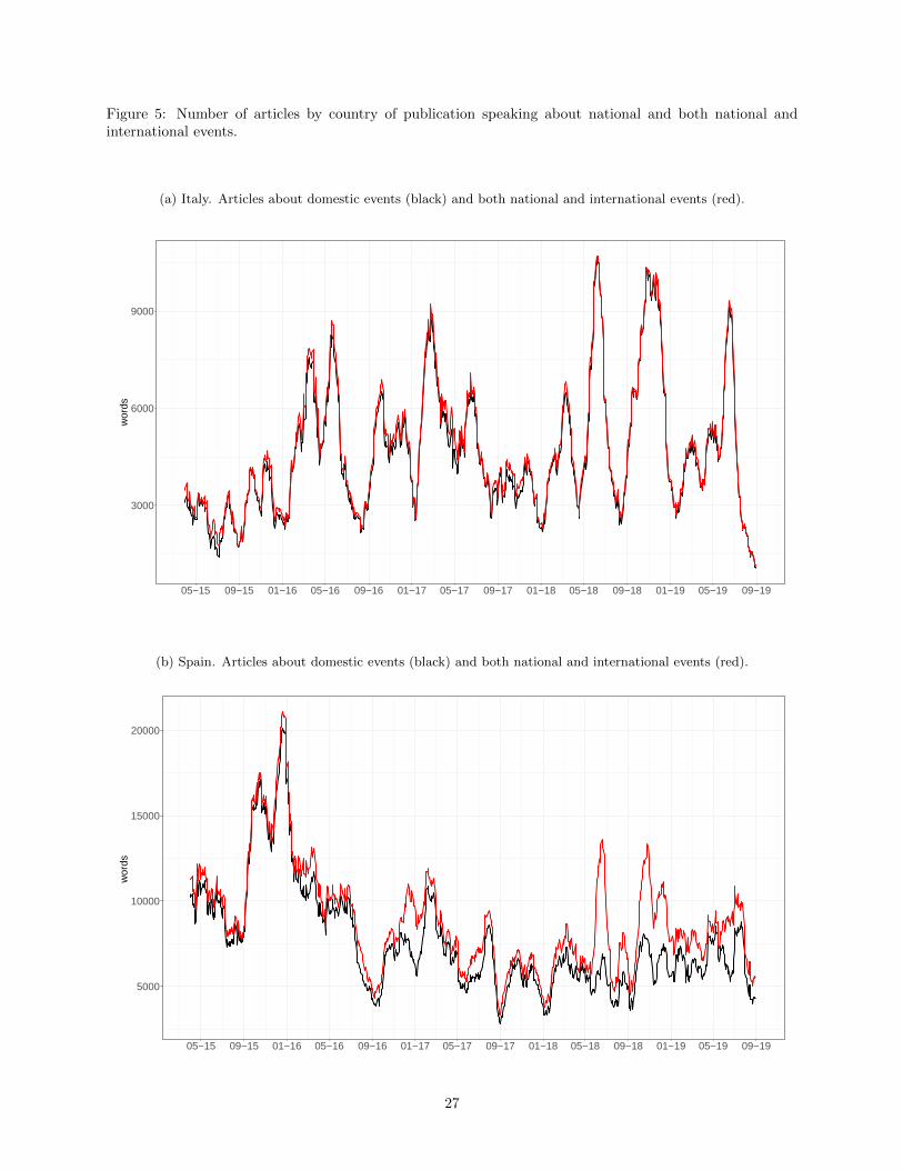
Figure 5: Number of articles by country of publication speaking about national and both national andinternational events.

(a) Italy. Articles about domestic events (black) and both national and international events (red).

3000

6000

9000

05−15 09−15 01−16 05−16 09−16 01−17 05−17 09−17 01−18 05−18 09−18 01−19 05−19 09−19

wor

ds

(b) Spain. Articles about domestic events (black) and both national and international events (red).

5000

10000

15000

20000

05−15 09−15 01−16 05−16 09−16 01−17 05−17 09−17 01−18 05−18 09−18 01−19 05−19 09−19

wor

ds

27

Figure 6: Distress (green) and panic (red) indicators extracted from GDELT economic news.

(a) Italy

0

5

10

15

05−15 09−15 01−16 05−16 09−16 01−17 05−17 09−17 01−18 05−18 09−18 01−19 05−19 09−19

wor

ds

(b) Spain

0

5

10

05−15 09−15 01−16 05−16 09−16 01−17 05−17 09−17 01−18 05−18 09−18 01−19 05−19 09−19

wor

ds

Notes: Solid lines refer to news on national events, dashed lines refer to news on national and international events.

28

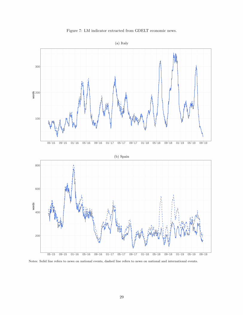
Figure 7: LM indicator extracted from GDELT economic news.

(a) Italy

100

200

300

05−15 09−15 01−16 05−16 09−16 01−17 05−17 09−17 01−18 05−18 09−18 01−19 05−19 09−19

wor

ds

(b) Spain

200

400

600

800

05−15 09−15 01−16 05−16 09−16 01−17 05−17 09−17 01−18 05−18 09−18 01−19 05−19 09−19

wor

ds

Notes: Solid line refers to news on national events, dashed line refers to news on national and international events.

29

Figure 8: Coefficients and confidence intervals from quantile regression estimation for Italy and Spain, whenvarying the quantile level q between 0.05 and 0.95.

(a) Italy

●

●●

●● ●

● ●● ● ● ● ● ● ● ●

● ●

●

●

●

● ● ●● ● ●

● ● ● ● ● ● ● ●●

●

●

Panic

Distress

0.05 0.15 0.25 0.35 0.45 0.55 0.65 0.75 0.85 0.95

−2

0

2

4

−2

0

2

4

(b) Spain

●

●● ● ●

●● ●

● ● ● ● ● ● ●●

● ●

●

● ● ●●

● ● ● ● ● ● ● ● ●● ● ●

●

●

●

Panic

Distress

0.05 0.15 0.25 0.35 0.45 0.55 0.65 0.75 0.85 0.95

0

1

0

1

Notes: In the graphs we report estimated coefficients and associated confidence intervals for βq on from Equation 2:

∆Spreadt+1 = αq + δq0∆Spreadt + δq1Xt + γqLMt−h + βqEmotiont−h + εt+1 with q = 0.05, 0.1, 0.15, ..., 0.95, for h = 0.

30

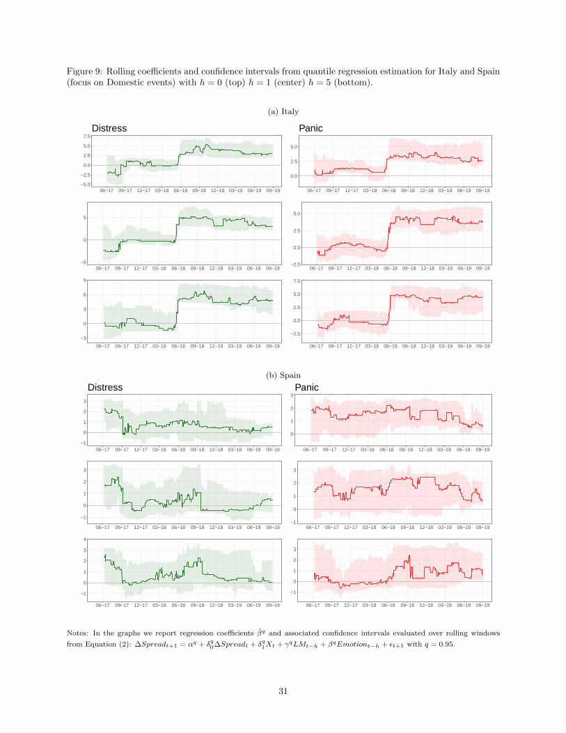
Figure 9: Rolling coefficients and confidence intervals from quantile regression estimation for Italy and Spain(focus on Domestic events) with h = 0 (top) h = 1 (center) h = 5 (bottom).

(a) Italy

−5.0

−2.5

0.0

2.5

5.0

7.5

06−17 09−17 12−17 03−18 06−18 09−18 12−18 03−19 06−19 09−19

Distress

0.0

2.5

5.0

06−17 09−17 12−17 03−18 06−18 09−18 12−18 03−19 06−19 09−19

Panic

−5

0

5

06−17 09−17 12−17 03−18 06−18 09−18 12−18 03−19 06−19 09−19−2.5

0.0

2.5

5.0

06−17 09−17 12−17 03−18 06−18 09−18 12−18 03−19 06−19 09−19

−3

0

3

6

9

06−17 09−17 12−17 03−18 06−18 09−18 12−18 03−19 06−19 09−19

−2.5

0.0

2.5

5.0

7.5

06−17 09−17 12−17 03−18 06−18 09−18 12−18 03−19 06−19 09−19

(b) Spain

−1

0

1

2

3

06−17 09−17 12−17 03−18 06−18 09−18 12−18 03−19 06−19 09−19

Distress

0

1

2

3

06−17 09−17 12−17 03−18 06−18 09−18 12−18 03−19 06−19 09−19

Panic

−1

0

1

2

3

06−17 09−17 12−17 03−18 06−18 09−18 12−18 03−19 06−19 09−19−1

0

1

2

3

06−17 09−17 12−17 03−18 06−18 09−18 12−18 03−19 06−19 09−19

−1

0

1

2

3

4

06−17 09−17 12−17 03−18 06−18 09−18 12−18 03−19 06−19 09−19

−1

0

1

2

3

06−17 09−17 12−17 03−18 06−18 09−18 12−18 03−19 06−19 09−19

Notes: In the graphs we report regression coefficients βq and associated confidence intervals evaluated over rolling windows

from Equation (2): ∆Spreadt+1 = αq + δq0∆Spreadt + δq1Xt + γqLMt−h + βqEmotiont−h + εt+1 with q = 0.95.

31

Figure 10: Rolling coefficients and confidence intervals from quantile regression estimation for Italy andSpain (Domestic and International events) with h = 0 (top) h = 1 (center) h = 5 (bottom).

(a) Italy

−5.0

−2.5

0.0

2.5

5.0

7.5

06−17 09−17 12−17 03−18 06−18 09−18 12−18 03−19 06−19 09−19

Distress

0.0

2.5

5.0

06−17 09−17 12−17 03−18 06−18 09−18 12−18 03−19 06−19 09−19

Panic

−5.0

−2.5

0.0

2.5

5.0

7.5

06−17 09−17 12−17 03−18 06−18 09−18 12−18 03−19 06−19 09−19−2.5

0.0

2.5

5.0

06−17 09−17 12−17 03−18 06−18 09−18 12−18 03−19 06−19 09−19

−3

0

3

6

9

06−17 09−17 12−17 03−18 06−18 09−18 12−18 03−19 06−19 09−19

−2

0

2

4

6

06−17 09−17 12−17 03−18 06−18 09−18 12−18 03−19 06−19 09−19

(b) Spain

−2

0

2

4

06−17 09−17 12−17 03−18 06−18 09−18 12−18 03−19 06−19 09−19

Distress

0

2

4

06−17 09−17 12−17 03−18 06−18 09−18 12−18 03−19 06−19 09−19

Panic

0

2

4

06−17 09−17 12−17 03−18 06−18 09−18 12−18 03−19 06−19 09−19

0

2

4

06−17 09−17 12−17 03−18 06−18 09−18 12−18 03−19 06−19 09−19

0

2

4

06−17 09−17 12−17 03−18 06−18 09−18 12−18 03−19 06−19 09−19

−2

0

2

06−17 09−17 12−17 03−18 06−18 09−18 12−18 03−19 06−19 09−19

Notes: In the graphs we report regression coefficients βq and associated confidence intervals evaluated over rolling windows

from Equation (2): ∆Spreadt+1 = αq + δq0∆Spreadt + δq1Xt + γqLMt−h + βqEmotiont−h + εt+1 with q = 0.95.

32

Figure 11: Rolling R2 for Italy (Domestic events) with h = 0 (top) h = 1 (center) h = 5 (bottom).

0.00

0.05

0.10

05−17 07−17 09−17 11−17 01−18 03−18 05−18 07−18 09−18 11−18 01−19 03−19 05−19 07−19 09−19

0.00

0.05

0.10

05−17 07−17 09−17 11−17 01−18 03−18 05−18 07−18 09−18 11−18 01−19 03−19 05−19 07−19 09−19

0.00

0.05

0.10

0.15

05−17 07−17 09−17 11−17 01−18 03−18 05−18 07−18 09−18 11−18 01−19 03−19 05−19 07−19 09−19

Notes: The rolling R2 displayed are calculated as a difference of the R2 for the regression ∆Spreadt+1 = αq + δq0∆Spreadt +

δq1Xt + γqLMt−h + βqEmotiont−h + εt+1 from the R2 of the benchmark model ∆Spreadt+1 = αq + δq0∆Spreadt + δq1Xt +

γqLMt−h + εt+1 where βq is set to zero and with q = 0.95. The red line is for Emotiont = Panict, the green line is

Emotiont = Distresst.

33

Figure 12: Rolling R2 for Spain (Domestic and international events) with h = 0 (top) h = 1 (center) h = 5(bottom).

0.00

0.02

0.04

0.06

0.08

05−17 07−17 09−17 11−17 01−18 03−18 05−18 07−18 09−18 11−18 01−19 03−19 05−19 07−19 09−19

0.00

0.02

0.04

0.06

05−17 07−17 09−17 11−17 01−18 03−18 05−18 07−18 09−18 11−18 01−19 03−19 05−19 07−19 09−19

0.00

0.01

0.02

0.03

05−17 07−17 09−17 11−17 01−18 03−18 05−18 07−18 09−18 11−18 01−19 03−19 05−19 07−19 09−19

Notes: The rolling R2 displayed are calculated as a difference of the R2 for the regression ∆Spreadt+1 = αq + δq0∆Spreadt +

δq1Xt + γqLMt−h + βqEmotiont−h + εt+1 from the R2 of the benchmark model ∆Spreadt+1 = αq + δq0∆Spreadt + δq1Xt +

γqLMt−h + εt+1 where βq is set to zero and with q = 0.95. The red line is for Emotiont = Panict, the green line is

Emotiont = Distresst.

34

Figure 13: Fluctuation test for Italy (Domestic events) with h = 1 (top) h = 5 (bottom).

−4

−2

0

2

03−18 05−18 07−18 09−18 11−18 01−19 03−19 05−19 07−19 09−19

−2

0

2

03−18 05−18 07−18 09−18 11−18 01−19 03−19 05−19 07−19 09−19

Notes: The Fluctuation test compares the forecasting performance of equation (2): ∆Spreadt+1 = αq + δq0∆Spreadt + δq1Xt +

γqLMt−h+βqEmotiont−h+εt+1 against the one of the benchmark model ∆Spreadt+1 = αq+δq0∆Spreadt+δq1Xt+γqLMt−h+

εt+1 where βq is set to zero and with q = 0.95. The red line is for Emotiont = Panict, the green line is Emotiont = Distresst.

Negative values indicate that model in equation (2) outperforms the benchmark model. The dashed line indicates the critical

value of the Fluctuation test statistic at the 5 per cent significance level. When the estimated test statistic is below the negative

critical value line, the model forecasts significantly better than the benchmark.

35

Figure 14: Fluctuation test for Spain (Domestic and international events) with h = 1 (top) h = 5 (bottom).

−2

0

2

03−18 05−18 07−18 09−18 11−18 01−19 03−19 05−19 07−19 09−19

−2

0

2

03−18 05−18 07−18 09−18 11−18 01−19 03−19 05−19 07−19 09−19

Notes: The Fluctuation test compares the forecasting performance of equation (2): ∆Spreadt+1 = αq + δq0∆Spreadt + δq1Xt +

γqLMt−h+βqEmotiont−h+εt+1 against the one of the benchmark model ∆Spreadt+1 = αq+δq0∆Spreadt+δq1Xt+γqLMt−h+

εt+1 where βq is set to zero and with q = 0.95. The red line is for Emotiont = Panict, the green line is Emotiont = Distresst.

Negative values indicate that model in equation (2) outperforms the benchmark model. The dashed line indicates the critical

value of the Fluctuation test statistic at the 5 per cent significance level. When the estimated test statistic is below the negative

critical value line, the model forecasts significantly better than the benchmark.

36

Appendix A

Below we report the list of outlets by country of origin that have been selected for the analysis.

Italy

Il Sole 24 Ore, Borsa Italiana, Italia Oggi, Milano Finanza, Ansa, il Giornale, Finanza, Wall Street Italia,

la Repubblica, Investire Oggi, Libero Quotidiano, il Messaggero Economia, il Fatto Quotidiano, il Corriere

della Sera, La Stampa Finanza, Huffington Post Italy, La Stampa, trend-online.com, teleborsa, tradelink, il

Tempo, finanza on-line, il Sussidiario.

Spain

ABC, El Mundo, El Pais, El Economista, Cincodias, Expansion, Libre mercado, Finanzas, Economia Finan-

zas, Bolsa, Info Bolsa, El Comercio, El dia, El progreso, El confidencial, El Confidencial Digital, Huffington

Post Spain, La razon, Negocios, El Diario.

37

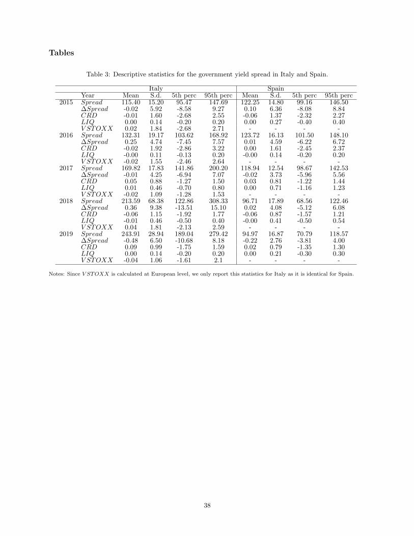
Tables

Table 3: Descriptive statistics for the government yield spread in Italy and Spain.

Italy SpainYear Mean S.d. 5th perc 95th perc Mean S.d. 5th perc 95th perc

2015 Spread 115.40 15.20 95.47 147.69 122.25 14.80 99.16 146.50∆Spread -0.02 5.92 -8.58 9.27 0.10 6.36 -8.08 8.84CRD -0.01 1.60 -2.68 2.55 -0.06 1.37 -2.32 2.27LIQ 0.00 0.14 -0.20 0.20 0.00 0.27 -0.40 0.40V STOXX 0.02 1.84 -2.68 2.71 - - - -

2016 Spread 132.31 19.17 103.62 168.92 123.72 16.13 101.50 148.10∆Spread 0.25 4.74 -7.45 7.57 0.01 4.59 -6.22 6.72CRD -0.02 1.92 -2.86 3.22 0.00 1.61 -2.45 2.37LIQ -0.00 0.11 -0.13 0.20 -0.00 0.14 -0.20 0.20V STOXX -0.02 1.55 -2.46 2.64 - - - -

2017 Spread 169.82 17.83 141.86 200.20 118.94 12.54 98.67 142.53∆Spread -0.01 4.25 -6.94 7.07 -0.02 3.73 -5.96 5.56CRD 0.05 0.88 -1.27 1.50 0.03 0.81 -1.22 1.44LIQ 0.01 0.46 -0.70 0.80 0.00 0.71 -1.16 1.23V STOXX -0.02 1.09 -1.28 1.53 - - - -

2018 Spread 213.59 68.38 122.86 308.33 96.71 17.89 68.56 122.46∆Spread 0.36 9.38 -13.51 15.10 0.02 4.08 -5.12 6.08CRD -0.06 1.15 -1.92 1.77 -0.06 0.87 -1.57 1.21LIQ -0.01 0.46 -0.50 0.40 -0.00 0.41 -0.50 0.54V STOXX 0.04 1.81 -2.13 2.59 - - - -

2019 Spread 243.91 28.94 189.04 279.42 94.97 16.87 70.79 118.57∆Spread -0.48 6.50 -10.68 8.18 -0.22 2.76 -3.81 4.00CRD 0.09 0.99 -1.75 1.59 0.02 0.79 -1.35 1.30LIQ 0.00 0.14 -0.20 0.20 0.00 0.21 -0.30 0.30V STOXX -0.04 1.06 -1.61 2.1 - - - -

Notes: Since V STOXX is calculated at European level, we only report this statistics for Italy as it is identical for Spain.

38