empirical guidance on scatterplot and dimension reduction ... · 2 2d, 3d, splom: justifications...

1077-2626/13/$31.00 © 2013 IEEE Published by the IEEE Computer Society

Accepted for publication by IEEE. ©2013 IEEE. Personal use of this material is permitted. Permission from IEEE must be obtained for all other uses, in any current or future media, including reprinting/republishing this material for advertising or promotional purposes, creating new collective works, for resale or redistribution to servers or lists, or reuse of any copyrighted component of this work in other works.

Empirical Guidance on Scatterplot and Dimension ReductionTechnique Choices

Michael Sedlmair, Member, IEEE, Tamara Munzner, Member, IEEE, and Melanie Tory

Abstract—To verify cluster separation in high-dimensional data, analysts often reduce the data with a dimension reduction (DR)technique, and then visualize it with 2D Scatterplots, interactive 3D Scatterplots, or Scatterplot Matrices (SPLOMs). With the goalof providing guidance between these visual encoding choices, we conducted an empirical data study in which two human codersmanually inspected a broad set of 816 scatterplots derived from 75 datasets, 4 DR techniques, and the 3 previously mentionedscatterplot techniques. Each coder scored all color-coded classes in each scatterplot in terms of their separability from other classes.We analyze the resulting quantitative data with a heatmap approach, and qualitatively discuss interesting scatterplot examples. Ourfindings reveal that 2D scatterplots are often ‘good enough’, that is, neither SPLOM nor interactive 3D adds notably more clusterseparability with the chosen DR technique. If 2D is not good enough, the most promising approach is to use an alternative DRtechnique in 2D. Beyond that, SPLOM occasionally adds additional value, and interactive 3D rarely helps but often hurts in terms ofpoorer class separation and usability. We summarize these results as a workflow model and implications for design. Our results offerguidance to analysts during the DR exploration process.

Index Terms—Dimensionality reduction, scatterplots, quantitative study

1 INTRODUCTION

High-dimensional data analysis is a common challenge amongst ex-perts from many application domains such as science, engineering orfinance. When conducting visual analysis of high-dimensional data,one typical approach is to transform the original dataset using a di-mensionality reduction (DR) technique to create a lower-dimensionalversion that preserves as much information as possible from the orig-inal, and then visually encode only the reduced data [34]. Many DRtechniques exist [45]; the most commonly used for visual data analysisinclude Principal Component Analysis (PCA) [22] and many variantsof Multidimensional Scaling (MDS) [5, 16]. The most common visualencoding (VE) technique for showing the dimensionally reduced datais scatterplots. The three major variants are static 2D scatterplots (ab-breviated here as 2D), interactive 3D scatterplots (i3D for short), andstatic 2D scatterplot matrices (SPLOMs) showing axis-aligned viewsfor every possible pair of reduced dimensions.

A significant amount of previous research has focused on provid-ing broad guidance for high-dimensional data analysis [1, 36, 38, 53],and some has focused more narrowly on guidance for DR in particu-lar [20]. However, there is insufficient empirical guidance on how tovisually encode dimensionally reduced data. Although the use of scat-terplots for non-reduced data has been extensively studied [29, 31],these findings focus on their use for judging correlation and thus donot generalize to their use with dimensionally reduced data becausethe new, synthetic dimensions are typically not correlated [34]. While2D scatterplots have been shown to be more effective than landscapesfor both visual search [40] and visual memory [41] tasks with dimen-sionally reduced data, the different scatterplot variants have not beencompared to each other for different types of datasets.

We conducted an empirical study to investigate the interplay be-tween visual encoding and dimensionality reduction techniques. Wecompared the three scatterplot VE variants (2D, i3D, and SPLOM)over 75 datasets reduced with four different DR techniques: PCA [22],

• Michael Sedlmair is with the University of Vienna. E-mail:[email protected].

• Tamara Munzner is with the University of British Columbia. E-mail:[email protected].

• Melanie Tory is with the University of Victoria. E-mail: [email protected].

Manuscript received 31 March 2013; accepted 1 August 2013; posted online13 October 2013; mailed on 4 October 2013.For information on obtaining reprints of this article, please sende-mail to: [email protected].

robust PCA [39], Glimmer MDS [21], and t-SNE [44]. In contrast toa typical user study collecting the judgements of a large number ofpeople over a small number of datasets, we conducted a data study tocollect judgements over a very broad set of data from a small numberof trained coders [35]. Two coders judged the class separation of 5460color-coded classes across 816 scatterplot visualizations.

We then engaged in generating a workflow model that can guidescatterplot choices in the DR exploration process. The workflowmodel reflects the main findings and implications of our study that2D is often ‘good enough’; that is, i3D and SPLOM do not notablyimprove visual class separability. If 2D is not good enough, the mostpromising approach is to keep the same visual encoding but to try an-other DR technique. Switching to a SPLOM as a next step does occa-sionally help. Switching to i3D, however, rarely helps and often hurts;that is, it has higher time costs and often provides less class separabil-ity, even for artificial datasets specifically designed for 3D.

This work is part of a larger project investigating questions at theintersection of DR and visualization. Our understanding of this inter-section is informed by a previous field study of DR and visualizationusage across multiple application domains, leading to a better under-standing of DR-related visual analysis tasks [34]. Here, we focus onthe task of visual cluster verification, one of several core tasks iden-tified in that work. The most direct precursor to this work was a tax-onomy of factors that contribute to visual cluster separation in scat-terplots with DR data [35]. The study presented here was conductedin parallel with the previous data study. It is based on the same setof 816 scatterplots and was conducted by the same two coders. De-spite these commonalities, however, the two studies are fundamentallydifferent: we gathered different data, used other analysis techniques,and pursued different research goals. For the cluster separation tax-onomy, we collected and analyzed qualitative characteristics, with thegoal of identifying how interactions between classes occurred within asingle scatterplot. For this work, we collected and analyzed quantita-tive judgements of class separation to compare between the scatterplotvariants of 2D, i3D, and SPLOM.

The primary contribution of this paper is the results of a data studyacross 816 scatterplots, featuring the comparison of three scatterplotvisual encoding techniques and four dimension reduction techniques.The secondary contribution is implications for design and usage ofscatterplots in visual data analysis with dimensionally reduced data,and an iterative workflow model to guide this use.

2 2D, 3D, SPLOM: JUSTIFICATIONS AND ASSUMPTIONS

Our study focuses on three scatterplot techniques: 2D, interactive3D, and scatterplot matrices. Reducing to 2 dimensions and using astatic 2D scatterplot is a very common practice [34]. However, an-other surprisingly frequent practice is reducing to three dimensionsand visually encoding with 3D scatterplots that are interactively in-spected [12, 13, 23], despite the known perceptual disadvantages ofvisualizing non-spatial, abstract data in 3D [9]. Our own previouswork has advocated the use of SPLOMs in conjunction with reducingto a moderate number of dimensions rather than assuming that eithertwo or three dimensions suffices for the reduced dimensionality [20].

A typical justification for the use of 3D scatterplots is that the in-trinsic dimensionality of a dataset is likely to be greater than 2; that is,that it would take more than just 2 dimensions to closely approximatethe information in the dataset. The scree plot analysis technique [20],where the fidelity of the reduced data to the original is plotted againstthe number of dimensions used, is a visual representation of exactlythis property: the intrinsic dimensionality of a dataset is estimated byfinding a knee in this curve.

Although estimating intrinsic dimensionality is a useful step in theDR analysis process, we focus on a somewhat different task: exam-ining the visual separation of clusters after visually encoding the re-duced data. We have observed that reducing to far fewer dimensionsthan the dataset’s intrinsic dimensionality often suffices to make clus-ters clearly visible after visually encoding. For example, a datasetwith an intrinsic dimensionality of 10 might have all of its clusters vi-sually separated even if it is reduced to 2 dimensions and shown witha single 2D scatterplot. We thus reaffirm Kruskal’s long-ago sugges-tion that the idea of appropriate dimensionality might be more usefulthan intrinsic dimensionality [25]. Our data study thus focuses on thequestion of the interplay between reducing to an appropriate dimen-sionality, and the VE technique used to show that reduced data.

A different rationale for the use of 3D scatterplots is that a choice ofreducing the original dataset to three dimensions dictates the choice ofvisually encoding that data using 3D. However, SPLOMs are an alter-native VE technique that can encode three dimensions of data into twospatial dimensions by trading off space for time; that is, they requiremore screen real estate than a single scatterplot, rather than requiringthat the user spend time interacting with them. Moreover, they can beused for more than three dimensions of data.

The idea that interaction imposes significant time cost has beennoted by many previous authors [26, 46]. We similarly argue that thereare different time costs to using the three scatterplot variants of 2D,i3D and SPLOMs. A single static 2D scatterplot has a very low timecost: all of the information is directly visible in one region without theneed to interact with the representation or mentally relate the views.A SPLOM has medium cost: there is no interaction, but a user mustswitch visual attention between regions and mentally relate the infor-mation in different views [26]. To our knowledge, the costs of using aSPLOM have not been studied empirically, but we conjecture that thiscost increases as the number of views within the SPLOM increase.The time cost of an interactive 3D scatterplot is high because the usermust spend significant time rotating the view to see the structure fromdifferent angles in order to see relationships hidden by occlusion inany single viewpoint. We conjecture that these interaction costs in 3Dare substantially higher than view-change costs in SPLOMs.

One obvious question is whether a SPLOM might also incur a timecost if a viewer needs time to mentally reconstruct overall shape fromaxis-aligned projections; in this case, the interaction support of i3Dwould probably reduce the cognitive load, and thus the total time cost,compared to a non-interactive SPLOM. We argue that shape recon-struction is similar to correlation: important for the general case ofnon-reduced data but not for the special case of reduced data. That is,it is not an important aspect for analysts engaged in the task of visualcluster separation with dimensionally reduced data.

These cost assumptions are based on an extensive body of workthat suggests the superiority of 2D visualizations over 3D ones fornon-spatial data [6, 8, 10, 30, 40, 41, 51]. We summarize this relatedwork in Section 3.1.

Based on this reasoning, we were skeptical that i3D would be avaluable visual encoding technique for DR data. We hypothesized thatthe less costly 2D and SPLOM VE techniques would be good enoughfor the majority of cases; that is, they would show the class structure ina sufficient way. Our analysis approach is based on the idea that whenmultiple VE techniques are good enough, the one with least time costis the best alternative.

3 RELATED WORK

We review related work on empirical evidence about 3D vs. 2D visu-alizations, and empirical studies and guidelines for high-dimensionaldata analysis involving DR.

3.1 3D vs. 2D: Empirical EvidenceOur work relies on the assertion that 3D scatterplots incur much higherinteraction costs than 2D ones. We do not test this assertion directly; itis based on a substantial body of empirical evidence about the appro-priateness of 2D and 3D representations for different tasks, of whichwe describe some below:

Three-dimensional visualizations, particularly 3D scatterplots, suf-fer from several limitations: occlusion of objects by other objects inthe scene [6, 37], scene complexity [6], depth ambiguity [30], perspec-tive distortion of distances and angles [37], and difficulty of interact-ing and navigating in 3D [30, 6, 51]. Clouds of disconnected pointsare perhaps one of the worst possible cases for 3D, since depth cuessuch as shadows and shape from shading [49] cannot be used.

2D and 3D visualizations have been experimentally compared fora wide variety of tasks and data types. For 3D spatial data and tasks,most empirical evidence suggests that interactive 3D visualizations of-ten outperform 2D projections [32, 37]. In terms of non-spatial data,however, there exists an extensive body of previous work that suggeststhat 2D visualizations are superior to interactive 3D [8, 10, 40, 41].DR data falls in the latter category of non-spatial data.

Our work specifically focuses on scatterplots. For scatterplots ofnon-DR data, there is some limited evidence that 3D may be help-ful for questions requiring integrated knowledge of 3 dimensions [52].(The data set used in this study was tiny by modern standards, withonly six data points.) However, we are interested only in scatterplotsof DR data, where there is substantial empirical evidence that 3D scat-terplots are ineffective. In a usability study of 3D DR scatterplots(with no comparison to 2D), Newby [30] reported that people couldmanage to use the 3D scatterplot representation to navigate an infor-mation space, but had difficulty judging distances between items andbecame disoriented when navigating through 3D space. Chalmers [6]similarly reported that a 3D point cloud representation of a documentspace suffered from occlusion, and users found it difficult to orientthemselves and navigate. In a direct comparison between 2D and 3Dscatterplots of DR data, Westerman and Cribbin [51] found that 2Doutperformed 3D for a search task. In fact, they reported that 2D wasas good or better than 3D even when the data variance accounted forby the 2D representation was only 50-70% of that of the 3D repre-sentation. Similarly, Fabrikant [14] demonstrated that 3D DR scat-terplots were ineffective compared to 2D DR scatterplots and 2D or3D information landscapes, for distance judgment and spatial arrange-ment tasks. A later study by Westerman et al. [50] on a browsing taskwas less conclusive, but showed that people needed to do significantlymore navigation in 3D compared to 2D, and were able to complete amore exhaustive search in 2D within approximately the same amountof time as 3D.

This paper provides complementary evidence that 3D scatterplotsare not suitable for cluster verification with DR data, from the per-spective of a data study rather than a user study.

3.2 DR: Studies and GuidanceThere is very little related work regarding empirical studies comparinghuman judgement of projections produced by different DR techniques.One notable exception is Lewis et al., who compared how experts andnovices judged the quality of 2D scatterplot projections from differentDR [28]. In a study with 36 participants, seven datasets and nine

DR techniques, they found that experts agreed in their DR judgementsbut novice users did not. While the focus of this study was on DRtechniques, user differences and a generic quality judging task, wespecifically focus on visual encodings of the data, on the breadth ofdatasets, and the interaction between VE and DR choices for visualcluster separation tasks.

On the other hand, there is a substantial body of previous workproviding guidelines for how to explore high-dimensional data usingscatterplots. Recent advances in the visualization literature specifi-cally have focused on finding interesting 2D scatterplots by computingand comparing a score for each 2D projection [36, 38, 53]. Wilkinsonet. al., for instance, specified nine measures to judge 2D projections,such as stringy, outlying or clumpy. More recently, similar approacheshave been proposed that were specifically designed for cluster verifi-cation tasks, that is, to find 2D projections that nicely separate pointsof given classes [1, 36, 38]. While these efforts focus on designingmeasures, our work aims to develop a workflow model to help userschoose among DR and VE techniques. In that sense, our work is sim-ilar in spirit to DimStiller [20], a system that provides workflows toguide steps in the high-dimensional data analysis process includingchoices on selecting and parameterizing DR techniques.

4 METHODS

To empirically evaluate visual encodings for DR data, we conducteda data study, where two trained coders inspected 816 scatterplot vi-sualizations and judged the visual separability of color-coded classesof these datasets. The study was conducted together with a previousdata study which was based on the same 816 scatterplots inspected bythe same two coders [35]. In our previous work, we reported on datathat we collected for qualitatively assessing class separation factorsand for evaluating automatic separation measures. Here, we analyze adifferent set of data we gathered, for which the two coders judged andquantified visual class separability.

We first explain how our research interest led to the methodologicalchoice of a data study. We then describe the data study in terms of ourguiding hypothesis, the 816 scatterplots, the data we gathered basedon these scatterplots, and how we analyzed this data.

4.1 Method RationaleOur methodological choice to conduct a data study was informed by along and thorough exploration of other evaluation methods.

Initially, we planned to conduct a user study in order to compare 2D,i3D and SPLOMs for DR data. However, we found that a user studywas not the right methodological approach for this research question;a pilot user study with five participants, six datasets and one DR tech-nique, revealed that the results strongly depended on the characteris-tics of the data as viewed in the scatterplots and not on differencesbetween participants. This finding suggested that it is imperative toinclude a broad set of dataset characteristics to make generalizableclaims; subjective differences and timing costs, as mainly tested intraditional user studies with many users and few datasets, are only ofmarginal interest for studying class separability across DR and VEchoices.

Judging class separability on a very broad set of datasets, DR tech-niques, and VE choices requires a significant amount of work. Wetherefore sought automatic class separation measures to conduct theseclass separability judgements. Such quality measures have gained re-cent attention [4] and researchers have proposed using them for eval-uation purposes [3]. We used two state-of-the-art measures to judgeclass separability for our study [36, 38], however, we found that theyproduced unreliable results. By comparing these automatic measuresto our human judgment, we identified strong discrepancies in classseparation judgments for half of our 816 scatterplots [35]. These fail-ure rates are not acceptable for our purposes.

Since reliable automatic separation measures were not available, wedecided to conduct a data study in which class separation is judged bya small number of trained human coders. This decision is supportedby recent empirical evidence that humans are consistent in their visualcluster evaluation tasks, especially if they are trained experts as in our

case [27]. Consistency among expert coders, or inter-coder reliability,is a crucial precondition for the methodological approach we took.

While conducting such studies with one coder is not uncommon,we followed the recommended practice of using two coders and as-sessing objectivity through inter-coder reliability. Given the significantworkload of such studies, more than two coders would be unusual.

4.2 Guiding HypothesisOur data collection and analysis was informed by a guiding hypothe-sis. We call it guiding to mean that it expressed our intuitions at thebeginning of this project, and not to reflect unambiguous and testablecause-effect relations. Our guiding hypothesis was that:• 2D is often good enough for showing visible class structure;• SPLOM sometimes adds more information;• i3D rarely provides additional benefits in real-world datasets,

but sometimes does for specifically designed synthetic datasets;• sometimes none of these visual encodings reveals visible class

structure.The major goals of our study were to get a better understanding of

how often these four situations occur, that is, the quantification of “of-ten”, “sometimes”, and “rarely”, and of how they change under differ-ent circumstances, such as choosing between different DR techniquesor for datasets with different characteristics.

4.3 Scatterplot samplesThe basis for the quantitative judgements of the coders was the sameset of 816 scatterplot samples that we generated for previous workin which coders made qualitative judgements about them [35]. Thesesamples resulted from the combination of 75 datasets reduced with 4DR techniques (PCA, Robust PCA, Glimmer MDS, and t-SNE) andvisualized with 3 scatterplot VE techniques (2D, i3D, and SPLOM).We call them scatterplot samples to emphasize that while the SPLOMcontains many individual scatterplots as subcomponents, we count theentire SPLOM as a single scatterplot sample rather than separatelyadding each subcomponent to the total. We summarize the generationprocess briefly here and provide further details in the supplementalmaterial.

We used a set of 75 datasets divided into four different cate-gories: 31 real datasets from our colleagues and collaborators [19,36, 38] or online data repositories [17, 33, 42, 47, 48]; 16 synthetic-gaussian datasets with 3 to 5 randomly distributed gaussian clusters;24 synthetic-entangled datasets with higher-dimensionally entangledclasses; and 4 synthetic-grid datasets that are simply regular high-dimensional grids, to provide a baseline of known and highly regu-lar dataset structure. Figure 5 shows examples of entangled datasets;these were specifically designed so that they could not be untangledwith linear DR techniques, and were intended to be the best possiblecase for 3D scatterplots.

These four categories are ordered from very realistic to highly artifi-cial, and are presented in this order throughout the paper. The datasetsranged from 77 to 43,500 points (median=500), from 3 to 159 originaldimensions (median=7), and between 2 and 53 classes (median=5).All datasets were pre-classified, either in our generation process, byusing clustering algorithms, or as provided with the data.

We carefully selected a set of four representative DR techniques toreduce these 75 datasets: The venerable PCA [22] technique, whichfinds linear projections based on variance, is the first choice of manyanalysts in the real world [34]. As PCA is known to be vulnerable tooutliers, we included another linear technique, Robust PCA [39] thathas been found to be tolerant of outliers. Given the limitations of linearDR techniques, we additionally included two non-linear techniques:Glimmer MDS [21] is a representative of the well-known family ofmultidimensional scaling techniques that seek to optimally map pointdistances from the high-dimensional space into a low-dimensionalprojection. The recent approach of t-Distributed Stochastic Neigh-bor Embedding (t-SNE) [44] is a non-linear DR approach specificallydesigned to separate clusters well—the task we are interested in.

The result of running these 4 DR techniques on the 75 datasets was272 dimension reduction operations rather than 300; in the remaining

28 cases, the computations did not complete because the techniqueassumptions were not met by the dataset characteristics. All computa-tions were done in R.

The dimensionally reduced data was then visually encoded withthree scatterplot techniques: 2D, i3D and SPLOMs. Points in all scat-terplot samples were color-coded based on the given class structure.For 2D scatterplots we reduced the data to two dimensions, and fori3D to three dimensions. For SPLOMs, we generated a set of n-waySPLOMs per dataset, where n is the number of dimensions shownin the SPLOM. The value of n ranged from 3 to dmax, a maximumvalue determined by a combination of the original dimensionality ofthe dataset and the values of class separation measures [36], with a capof 15 dimensions as the upper limit. We introduced this cap to keep thestudy manageable in terms of time costs for the coders. From this setof SPLOMs, each coder individually selected one SPLOM for the datacollection process, by making a judgement about when adding moredimensions to the SPLOM stopped providing any benefits in terms ofclass separation. The outcome of this process was a set of 816 scatter-plot samples.

4.4 Data Collection

The data collection was conducted by the same two trained coders1

and in parallel with the study in our previous work [35]. For the studyreported here, the coders used their in-depth manual inspection of 816scatterplot samples to rate how visually separable each of the color-coded classes were within these scatterplots. Data gathering took twomonths, with a total of approximately 80 hours of coding time foreach person. In the first six weeks, the coders met two to four timesa week to discuss many scatterplot samples and iteratively adapt thecoding schemes and strategies, re-coding samples as necessary as theschemes changed. This iterative development of the coding scheme isa lengthly process but is crucial for scientific rigor [7, 18].

With the number of classes being variable across datasets, eachcoder made a total of 5460 classwise ratings. Each of these classeswas given a score between 1 and 5, where 1 means the class is notseparated at all and 5 means the class is nicely separated. Initially, wehad only three categories, but in the iterative coding process we foundthat a 3-point scale did not provide enough depth for representing theseparability of clusters.

Figure 1 shows examples of different classes and how they werejudged by the coders. The coders’ definition of visual class separabil-ity followed our previously proposed taxonomy of visual cluster sep-aration factors [35]. The most important separability factors we tookinto account were the amount of spatial overlap between classes andfactors related to connectedness between points of a class. A classof points that is connected to each other and that has no overlap withany other class, for instance, gets a “5”. Larger spatial overlaps anddisconnectedness of points reduce the score. Our manual coding wasalso robust with respect to a variety of factors that are not reliablytestable with state-of-the-art separation measures, such as the shapeof a class, the variance of size, point count or point density betweenclasses. That is, as long as a class is connected and without overlay,its shape, size, point count, or density had no negative impact on itsrating score. Classes with only 1 point were not judged because theseparation of a one-point class is not meaningful. The supplementalmaterial contains a full set of all examples and ratings.

To asses the objectivity of these class-wise ratings, we computedthe inter-coder reliability using Krippendorff’s alpha. In contrast toother inter-coder measures, Krippendorff’s alpha can be used for anynumber of coders, is robust to missing values, and works with dif-ferent data types such as nominal, ordinal or ratio; for our classwiseratings Krippendorff’s alpha was 0.858 for ordinal data; a score of .8or greater is considered acceptable in most situations [24].

We also recorded other data that we intended to use to address ourresearch questions. In particular, the coders additionally recorded theirsubjective preference of (a) which combinations of DR and VE they

1One of the coders is the first author of this paper, as is standard practicewith the methodological approach we took.

−1.0 −0.5 0.0 0.5 1.0

−1.0

−0.5

0.0

0.5

1.0

.x

.y

(a) max sep: (5,5,5)−2 −1 0 1 2 3

−4−2

02

.x

.y

(b) no sep: (1,1,1)−1.0 −0.5 0.0 0.5 1.0

−1.0

−0.5

0.0

0.5

1.0

.x

.y

(c) mixed: (4,3,2,1)

Fig. 1. 2D scatterplot samples and class codings from the data study.(a) entangled3-m-3d-smallOverlap reduced with PCA represent-ing three classes that were each coded as 5, nicely separated; (b)gauss-n100-5d-3largeCl reduced with Glimmer MDS represent-ing three classes that were each coded as 1, not separated at all. (c)entangled2-4d-overlap reduced with robust PCA showing an ex-ample in between these: the green class got a 4, the red class a 3, theblue class a 2, and the black class, which is completely mixed with theother classes, a 1. Both coders agreed on all these ratings. As with allfollowing scatterplot figures, point sizes have been increased for easierreadability in the paper.

considered the best for each dataset, and (b) which VE they foundmost helpful for a dataset ×DR combination2. However, this datashowed effects of personal preference, with Krippendorff’s alpha for(a) being 0.32 and for (b) 0.461. In particular, we found that one codertended to subjectively pick 3D scatterplots, and the other one tendedto prefer 2D and SPLOM. We therefore excluded this data from ouranalysis. However, as shown above, the low-level classwise ratingswere resistant to such subjective biases and provide therefore reliableand un-biased data for our methodological approach.

4.5 Data Analysis

We undertook extensive exploratory analysis of the collected data. Wereport only the most interesting results here.

The analysis in Sections 5.1 through 5.3 is primarily presentedusing heatmaps that either directly show the classwise ratings orshow derived data about differences between VE and DR techniques.Heatmaps in the paper show averaged ratings of both coders; the sup-plemental material contains larger and labeled versions of these aver-aged heatmaps, as well as separate heatmaps for each coder. We usedthese representations for our own exploratory analysis and found themvery useful. They make visible as many of the class-wise ratings aspossible, and allow readers to make their own judgements about thedata at both overview and detail levels. Moreover, we also did notwant to impose our own opinion of what constitutes ‘better’. For in-stance, is a ‘better’ VE one where at least one class is more separable,or one where more classes improve than decline? To allow for suchdiffering interpretations, we decided to show the rating data that wegathered in as much detail as possible.

We complemented the heatmap analysis with inferential statistics.Because our rating data are ordinal and not normally distributed, weused the non-parametric Wilcoxon signed rank test (two tailed). Bon-ferroni correction was applied within each group of tests.

We used the results of the quantitative analysis to select a set ofinteresting example scatterplots for further qualitative discussion; thesupplemental material again contains more of these examples. Ourdata analysis is thus in the spirit of mixed methods approaches [11].

5 RESULTS AND DISCUSSION

We first present the base data from the averaged classwise ratings. Wethen present the within-DR analysis of the data for each of the four DRtechniques separately, followed by the cross-DR analysis across all ofthem together. After a quantification of results into the four bins givenby our guiding hypothesis, we briefly discuss secondary results on theusage of SPLOMs that support our usability assumption.

2(a) was collected as nominal data, and (b) as ordinal rankings.

abalone 1.0 1.0 1.0 1.0 1.0 1.0 1.0 1.0 1.0 1.0 1.0 1.0 1.0 1.0 1.0 1.0 NA 1.0 1.0 1.0 1.0 1.0 1.0 1.0 1.0 1.0 1.0 1.0 1.0 1.0 1.0 1.0 1.0 NA 1.0 1.0 1.0 1.0 1.0 1.0 1.0 1.0 1.0 1.0 1.0 1.0 1.0 1.0 1.0 1.0 NA NA NA NA NA NA NA NA NA NA NA NA NA NA NA NA NA NA

cars03Cropped_d2 1.0 1.0 1.0 1.0 1.0 1.0 1.0 1.0 1.0 1.0 1.0 1.0 1.0 1.0 1.0 1.0 NA 1.0 1.0 1.0 1.0 1.0 1.0 1.0 1.0 1.0 1.0 1.0 1.0 1.0 1.0 1.0 1.0 NA 1.0 1.0 1.0 1.0 1.0 1.0 1.0 1.0 1.0 1.0 1.0 1.0 1.0 1.0 1.0 1.0 NA NA NA NA NA NA NA NA NA NA NA NA NA NA NA NA NA

italianwines 1.0 1.0 1.0 1.0 1.0 1.0 1.0 1.0 1.0 1.0 1.0 1.0 1.0 NA NA NA NA 1.0 1.0 1.0 1.0 1.0 1.0 1.0 1.0 1.0 1.0 1.0 1.0 1.0 NA NA NA NA 1.5 1.0 1.0 1.5 1.0 1.0 1.5 2.0 2.0 1.0 2.0 4.0 3.5 NA NA NA NA 2.0 1.0 1.0 1.0 1.0 2.0 1.5 1.0 1.0 1.0 2.0 2.0 2.0 NA NA NA NA

worldmap 5.0 5.0 3.0 4.0 99.0 5.0 5.0 3.0 5.0 2.5 4.0 5.0 5.0 NA NA NA NA 5.0 5.0 5.0 3.0 99.0 2.0 4.0 2.0 3.5 4.5 5.0 5.0 3.0 NA NA NA NA 1.0 4.5 5.0 5.0 99.0 5.0 5.0 2.0 5.0 5.0 5.0 5.0 5.0 NA NA NA NA 5.0 5.0 5.0 5.0 99.0 5.0 5.0 5.0 5.0 5.0 5.0 5.0 4.0 NA NA NA NA

cars03Cropped_d3 1.0 2.0 1.0 2.0 1.0 1.0 1.5 1.0 3.0 3.0 1.0 2.5 NA NA NA NA NA 1.0 1.0 1.0 2.0 1.0 1.0 1.0 1.0 1.0 1.0 1.0 1.0 NA NA NA NA NA 1.0 1.0 1.0 1.0 1.0 1.0 1.0 1.0 1.0 2.5 1.0 1.0 NA NA NA NA NA NA NA NA NA NA NA NA NA NA NA NA NA NA NA NA NA NA

fisheries_clusteredByEscapementTarget 1.0 1.0 1.0 1.0 1.0 1.0 1.0 1.0 1.0 1.0 1.0 NA NA NA NA NA NA 4.5 4.5 4.5 4.5 4.5 4.5 4.5 4.5 4.5 4.5 4.5 NA NA NA NA NA NA 2.5 3.5 3.5 3.5 4.0 4.5 4.5 4.5 4.5 4.5 4.5 NA NA NA NA NA NA 1.5 2.5 2.5 2.5 2.5 1.5 2.5 2.5 1.5 1.5 2.0 NA NA NA NA NA NA

fisheries_clusteredByHarvestRule 5.0 4.5 3.0 1.0 1.0 1.0 1.0 1.0 1.0 1.0 1.0 NA NA NA NA NA NA 5.0 4.5 3.0 1.0 1.0 1.0 1.0 1.0 1.0 1.0 1.0 NA NA NA NA NA NA 5.0 5.0 5.0 5.0 5.0 5.0 5.0 5.0 5.0 5.0 5.0 NA NA NA NA NA NA 5.0 5.0 5.0 4.0 3.5 3.5 3.5 3.5 3.5 3.0 3.0 NA NA NA NA NA NA

yeast 1.0 1.0 1.0 1.0 1.0 2.0 1.5 1.0 1.0 1.0 NA NA NA NA NA NA NA NA NA NA NA NA NA NA NA NA NA NA NA NA NA NA NA NA NA NA NA NA NA NA NA NA NA NA NA NA NA NA NA NA NA NA NA NA NA NA NA NA NA NA NA NA NA NA NA NA NA NA

ecoliproteins 4.0 3.0 1.0 1.0 2.0 1.5 1.0 2.5 NA NA NA NA NA NA NA NA NA NA NA NA NA NA NA NA NA NA NA NA NA NA NA NA NA NA 4.0 2.0 1.0 1.0 2.0 2.0 5.0 2.0 NA NA NA NA NA NA NA NA NA NA NA NA NA NA NA NA NA NA NA NA NA NA NA NA NA NA

efashion 1.0 1.0 1.0 1.0 1.5 1.0 1.0 2.0 NA NA NA NA NA NA NA NA NA 1.0 1.0 1.0 1.0 1.5 1.0 1.0 2.0 NA NA NA NA NA NA NA NA NA 1.0 1.0 1.0 1.0 1.5 1.0 1.0 1.5 NA NA NA NA NA NA NA NA NA NA NA NA NA NA NA NA NA NA NA NA NA NA NA NA NA NA

tse300 4.5 4.0 3.0 4.5 4.5 2.5 4.0 99.0 NA NA NA NA NA NA NA NA NA 4.5 4.0 2.5 4.5 4.5 2.5 4.0 99.0 NA NA NA NA NA NA NA NA NA 5.0 2.5 2.5 2.5 5.0 1.5 1.5 99.0 NA NA NA NA NA NA NA NA NA 1.0 1.0 1.0 1.0 1.0 1.0 1.0 99.0 NA NA NA NA NA NA NA NA NA

cereal 1.0 1.0 1.0 1.0 1.0 1.0 1.0 NA NA NA NA NA NA NA NA NA NA NA NA NA NA NA NA NA NA NA NA NA NA NA NA NA NA NA 1.0 1.0 1.0 1.0 1.0 1.0 1.0 NA NA NA NA NA NA NA NA NA NA 1.0 1.0 1.0 1.0 1.0 1.0 1.0 NA NA NA NA NA NA NA NA NA NA

shuttle_big 1.0 1.0 1.0 1.0 1.0 1.5 1.5 NA NA NA NA NA NA NA NA NA NA NA NA NA NA NA NA NA NA NA NA NA NA NA NA NA NA NA 1.0 1.0 1.0 1.5 1.5 1.0 1.0 NA NA NA NA NA NA NA NA NA NA NA NA NA NA NA NA NA NA NA NA NA NA NA NA NA NA NA

shuttle_small 1.5 1.0 1.0 1.0 1.5 5.0 5.0 NA NA NA NA NA NA NA NA NA NA NA NA NA NA NA NA NA NA NA NA NA NA NA NA NA NA NA 1.0 1.0 1.0 2.0 1.5 2.0 1.5 NA NA NA NA NA NA NA NA NA NA NA NA NA NA NA NA NA NA NA NA NA NA NA NA NA NA NA

musicnetgroups 99.0 5.0 99.0 4.0 5.0 5.0 NA NA NA NA NA NA NA NA NA NA NA 99.0 5.0 99.0 5.0 5.0 5.0 NA NA NA NA NA NA NA NA NA NA NA 99.0 5.0 99.0 3.5 4.0 5.0 NA NA NA NA NA NA NA NA NA NA NA 99.0 5.0 99.0 1.0 1.0 2.5 NA NA NA NA NA NA NA NA NA NA NA

hiv NA NA NA NA NA NA NA NA NA NA NA NA NA NA NA NA NA NA NA NA NA NA NA NA NA NA NA NA NA NA NA NA NA NA 2.0 1.5 1.0 2.5 1.0 99.0 NA NA NA NA NA NA NA NA NA NA NA 1.0 1.5 2.0 3.0 1.0 99.0 NA NA NA NA NA NA NA NA NA NA NA

bbdm13 4.0 3.0 1.0 2.0 3.0 NA NA NA NA NA NA NA NA NA NA NA NA NA NA NA NA NA NA NA NA NA NA NA NA NA NA NA NA NA 1.0 1.0 1.0 1.0 1.0 NA NA NA NA NA NA NA NA NA NA NA NA 1.5 1.0 1.0 1.0 1.0 NA NA NA NA NA NA NA NA NA NA NA NA

white_ballance 1.0 1.0 3.0 1.5 2.5 NA NA NA NA NA NA NA NA NA NA NA NA 1.0 1.0 3.0 1.0 2.5 NA NA NA NA NA NA NA NA NA NA NA NA 1.0 2.0 2.5 1.0 2.0 NA NA NA NA NA NA NA NA NA NA NA NA NA NA NA NA NA NA NA NA NA NA NA NA NA NA NA NA NA

world_11d 4.5 2.5 1.5 3.0 4.0 NA NA NA NA NA NA NA NA NA NA NA NA 4.5 3.5 1.0 2.5 2.5 NA NA NA NA NA NA NA NA NA NA NA NA 5.0 4.0 3.5 3.0 4.5 NA NA NA NA NA NA NA NA NA NA NA NA 2.5 2.5 1.0 2.0 2.5 NA NA NA NA NA NA NA NA NA NA NA NA

world_9d 3.0 2.0 1.0 3.0 3.5 NA NA NA NA NA NA NA NA NA NA NA NA NA NA NA NA NA NA NA NA NA NA NA NA NA NA NA NA NA 4.0 3.5 4.5 2.5 4.5 NA NA NA NA NA NA NA NA NA NA NA NA 1.0 1.0 1.0 1.0 1.5 NA NA NA NA NA NA NA NA NA NA NA NA

boston 3.5 2.0 1.0 NA NA NA NA NA NA NA NA NA NA NA NA NA NA 4.0 2.5 1.0 NA NA NA NA NA NA NA NA NA NA NA NA NA NA 4.5 3.5 4.0 NA NA NA NA NA NA NA NA NA NA NA NA NA NA 5.0 3.0 4.0 NA NA NA NA NA NA NA NA NA NA NA NA NA NA

iris 5.0 5.0 5.0 NA NA NA NA NA NA NA NA NA NA NA NA NA NA 5.0 4.5 4.5 NA NA NA NA NA NA NA NA NA NA NA NA NA NA 5.0 4.0 4.0 NA NA NA NA NA NA NA NA NA NA NA NA NA NA 5.0 2.5 2.5 NA NA NA NA NA NA NA NA NA NA NA NA NA NA

olive 3.0 5.0 3.5 NA NA NA NA NA NA NA NA NA NA NA NA NA NA 3.0 5.0 3.5 NA NA NA NA NA NA NA NA NA NA NA NA NA NA 4.5 5.0 4.5 NA NA NA NA NA NA NA NA NA NA NA NA NA NA 5.0 5.0 5.0 NA NA NA NA NA NA NA NA NA NA NA NA NA NA

swanson 1.0 1.0 2.0 NA NA NA NA NA NA NA NA NA NA NA NA NA NA NA NA NA NA NA NA NA NA NA NA NA NA NA NA NA NA NA 1.0 1.0 1.0 NA NA NA NA NA NA NA NA NA NA NA NA NA NA 1.0 1.0 2.5 NA NA NA NA NA NA NA NA NA NA NA NA NA NA

wine 3.5 2.0 2.0 NA NA NA NA NA NA NA NA NA NA NA NA NA NA 4.5 2.0 2.0 NA NA NA NA NA NA NA NA NA NA NA NA NA NA 4.0 3.5 4.5 NA NA NA NA NA NA NA NA NA NA NA NA NA NA 4.5 3.0 3.5 NA NA NA NA NA NA NA NA NA NA NA NA NA NA

breast-cancer-wisconsin 4.0 4.0 NA NA NA NA NA NA NA NA NA NA NA NA NA NA NA NA NA NA NA NA NA NA NA NA NA NA NA NA NA NA NA NA 4.0 4.0 NA NA NA NA NA NA NA NA NA NA NA NA NA NA NA 3.5 3.0 NA NA NA NA NA NA NA NA NA NA NA NA NA NA NA

cars03Cropped_d1 3.0 3.0 NA NA NA NA NA NA NA NA NA NA NA NA NA NA NA 4.5 4.5 NA NA NA NA NA NA NA NA NA NA NA NA NA NA NA 3.0 3.0 NA NA NA NA NA NA NA NA NA NA NA NA NA NA NA NA NA NA NA NA NA NA NA NA NA NA NA NA NA NA NA NA

ionosphere 2.0 2.0 NA NA NA NA NA NA NA NA NA NA NA NA NA NA NA NA NA NA NA NA NA NA NA NA NA NA NA NA NA NA NA NA NA NA NA NA NA NA NA NA NA NA NA NA NA NA NA NA NA 2.5 2.5 NA NA NA NA NA NA NA NA NA NA NA NA NA NA NA

parkinsons_abs_croped 1.5 2.0 NA NA NA NA NA NA NA NA NA NA NA NA NA NA NA 1.5 2.0 NA NA NA NA NA NA NA NA NA NA NA NA NA NA NA 3.0 3.5 NA NA NA NA NA NA NA NA NA NA NA NA NA NA NA NA NA NA NA NA NA NA NA NA NA NA NA NA NA NA NA NA

spambase 1.5 2.0 NA NA NA NA NA NA NA NA NA NA NA NA NA NA NA NA NA NA NA NA NA NA NA NA NA NA NA NA NA NA NA NA 1.5 1.5 NA NA NA NA NA NA NA NA NA NA NA NA NA NA NA NA NA NA NA NA NA NA NA NA NA NA NA NA NA NA NA NA

wdbc_class_1_2 3.5 3.5 NA NA NA NA NA NA NA NA NA NA NA NA NA NA NA 4.0 4.0 NA NA NA NA NA NA NA NA NA NA NA NA NA NA NA 4.0 4.0 NA NA NA NA NA NA NA NA NA NA NA NA NA NA NA 1.5 2.0 NA NA NA NA NA NA NA NA NA NA NA NA NA NA NA

n100-d10-c5-spr0.1-out0 4.0 5.0 5.0 5.0 4.0 NA NA NA NA NA NA NA NA NA NA NA NA 1.0 5.0 1.0 5.0 1.0 NA NA NA NA NA NA NA NA NA NA NA NA 2.0 3.0 2.0 2.5 1.5 NA NA NA NA NA NA NA NA NA NA NA NA 3.5 4.5 4.0 3.5 3.5 NA NA NA NA NA NA NA NA NA NA NA NA








n100-d10-c3-spr0.1-out0 5.0 5.0 5.0 NA NA NA NA NA NA NA NA NA NA NA NA NA NA 5.0 5.0 5.0 NA NA NA NA NA NA NA NA NA NA NA NA NA NA 5.0 4.5 5.0 NA NA NA NA NA NA NA NA NA NA NA NA NA NA 3.5 3.0 4.0 NA NA NA NA NA NA NA NA NA NA NA NA NA NA








interleaved_100_200_15d_0_notcramped_notrotated 3.0 2.5 1.0 1.0 2.0 3.5 1.0 2.5 1.0 3.0 1.5 1.0 3.0 1.5 3.5 NA NA 2.5 2.5 1.0 1.0 1.5 4.0 1.0 2.5 1.0 3.5 1.5 1.0 3.5 1.5 4.0 NA NA 1.0 1.0 1.0 1.0 1.0 1.0 1.0 1.0 1.0 1.0 1.0 1.0 1.0 1.0 1.0 NA NA 5.0 5.0 5.0 5.0 5.0 5.0 5.0 5.0 5.0 5.0 5.0 5.0 5.0 5.0 5.0 NA NA

interleaved_100_200_15d_25_cramped_rotated 1.0 3.0 1.0 3.5 1.0 1.0 1.0 1.0 1.0 3.0 2.0 2.0 2.0 2.0 3.5 NA NA 1.0 3.0 1.0 3.5 1.0 1.0 1.0 1.0 1.0 3.0 2.0 2.0 2.0 2.0 3.5 NA NA 1.0 1.0 1.0 1.0 1.0 1.0 1.0 1.0 1.0 1.0 1.0 1.0 1.0 1.0 1.0 NA NA 5.0 5.0 5.0 5.0 5.0 4.0 5.0 5.0 5.0 5.0 5.0 5.0 5.0 4.0 5.0 NA NA

interleaved_100_200_10d_0_notcramped_notrotated 4.5 5.0 3.0 5.0 1.0 1.0 3.0 4.5 1.5 1.5 NA NA NA NA NA NA NA 4.0 5.0 3.0 5.0 1.0 1.0 3.0 4.5 1.5 1.0 NA NA NA NA NA NA NA 2.0 3.0 1.5 3.0 1.5 1.5 1.5 3.0 1.5 1.5 NA NA NA NA NA NA NA 5.0 5.0 4.5 5.0 5.0 5.0 5.0 5.0 5.0 5.0 NA NA NA NA NA NA NA

interleaved_100_200_10d_25_cramped_rotated 2.5 3.0 2.0 1.0 2.5 4.0 2.5 4.0 4.0 1.0 NA NA NA NA NA NA NA 2.5 2.5 2.0 1.0 2.0 4.0 2.5 4.0 4.0 1.0 NA NA NA NA NA NA NA 1.0 1.0 1.5 1.0 1.0 1.0 1.5 1.0 1.0 1.0 NA NA NA NA NA NA NA 5.0 5.0 5.0 5.0 5.0 5.0 5.0 5.0 5.0 5.0 NA NA NA NA NA NA NA

interleaved_100_200_6d_0_notcramped_notrotated 2.0 2.5 3.0 3.5 2.5 4.5 NA NA NA NA NA NA NA NA NA NA NA 2.0 3.5 3.0 3.0 3.0 4.5 NA NA NA NA NA NA NA NA NA NA NA 1.0 3.5 3.5 2.0 2.5 4.5 NA NA NA NA NA NA NA NA NA NA NA 4.5 4.5 5.0 4.0 4.0 4.5 NA NA NA NA NA NA NA NA NA NA NA

interleaved_100_200_6d_25_cramped_rotated 4.0 3.0 2.5 4.0 4.0 2.5 NA NA NA NA NA NA NA NA NA NA NA 4.0 3.0 2.5 4.0 4.0 2.5 NA NA NA NA NA NA NA NA NA NA NA 3.5 3.0 2.5 3.0 3.5 2.5 NA NA NA NA NA NA NA NA NA NA NA 4.0 4.5 3.5 4.5 4.5 4.0 NA NA NA NA NA NA NA NA NA NA NA

interleaved_100_200_5d_0_notcramped_notrotated 2.5 3.0 3.0 3.5 3.5 NA NA NA NA NA NA NA NA NA NA NA NA 2.5 3.5 3.0 3.5 3.5 NA NA NA NA NA NA NA NA NA NA NA NA 4.5 1.5 3.5 3.0 3.0 NA NA NA NA NA NA NA NA NA NA NA NA 4.5 4.5 4.5 4.5 4.5 NA NA NA NA NA NA NA NA NA NA NA NA

interleaved_100_200_5d_25_cramped_rotated 3.5 3.0 3.5 4.0 4.0 NA NA NA NA NA NA NA NA NA NA NA NA 3.0 3.0 4.0 4.0 4.0 NA NA NA NA NA NA NA NA NA NA NA NA 2.5 2.5 3.5 3.5 1.5 NA NA NA NA NA NA NA NA NA NA NA NA 3.5 4.5 4.0 4.5 4.5 NA NA NA NA NA NA NA NA NA NA NA NA

JavierGeneratedData_3dinterleaved_5classes 4.0 4.0 5.0 4.0 5.0 NA NA NA NA NA NA NA NA NA NA NA NA 4.5 4.5 4.0 4.5 4.0 NA NA NA NA NA NA NA NA NA NA NA NA 4.0 4.0 5.0 4.0 5.0 NA NA NA NA NA NA NA NA NA NA NA NA 4.5 5.0 5.0 5.0 5.0 NA NA NA NA NA NA NA NA NA NA NA NA

interleaved_100_200_4d_0_notcramped_notrotated 4.0 4.0 4.0 3.0 NA NA NA NA NA NA NA NA NA NA NA NA NA 4.0 4.0 4.0 3.0 NA NA NA NA NA NA NA NA NA NA NA NA NA 3.5 3.0 3.5 2.0 NA NA NA NA NA NA NA NA NA NA NA NA NA 4.5 5.0 4.5 3.0 NA NA NA NA NA NA NA NA NA NA NA NA NA

interleaved_100_200_4d_25_cramped_rotated 1.0 3.0 2.0 4.0 NA NA NA NA NA NA NA NA NA NA NA NA NA 1.0 3.0 2.0 4.0 NA NA NA NA NA NA NA NA NA NA NA NA NA 3.5 4.0 2.0 3.5 NA NA NA NA NA NA NA NA NA NA NA NA NA 3.5 4.0 4.0 4.5 NA NA NA NA NA NA NA NA NA NA NA NA NA

JavierGeneratedData_3dinterleaved_4classes 4.5 4.5 5.0 4.5 NA NA NA NA NA NA NA NA NA NA NA NA NA 4.5 4.0 4.5 4.0 NA NA NA NA NA NA NA NA NA NA NA NA NA 5.0 5.0 5.0 5.0 NA NA NA NA NA NA NA NA NA NA NA NA NA 5.0 5.0 5.0 5.0 NA NA NA NA NA NA NA NA NA NA NA NA NA

interleaved_100_500_3_25_cramped_rotated 4.5 4.5 4.5 NA NA NA NA NA NA NA NA NA NA NA NA NA NA 4.5 4.5 4.5 NA NA NA NA NA NA NA NA NA NA NA NA NA NA 4.5 4.5 4.5 NA NA NA NA NA NA NA NA NA NA NA NA NA NA 4.5 4.5 4.0 NA NA NA NA NA NA NA NA NA NA NA NA NA NA

interleaved_250_500_3_0_notCramped_rotated 5.0 5.0 5.0 NA NA NA NA NA NA NA NA NA NA NA NA NA NA 5.0 5.0 5.0 NA NA NA NA NA NA NA NA NA NA NA NA NA NA 5.0 5.0 5.0 NA NA NA NA NA NA NA NA NA NA NA NA NA NA 4.5 4.5 4.0 NA NA NA NA NA NA NA NA NA NA NA NA NA NA

JavierGeneratedData_3dinterleaved_3classes 4.5 4.5 4.5 NA NA NA NA NA NA NA NA NA NA NA NA NA NA 4.5 4.5 4.5 NA NA NA NA NA NA NA NA NA NA NA NA NA NA 5.0 5.0 5.0 NA NA NA NA NA NA NA NA NA NA NA NA NA NA 5.0 5.0 5.0 NA NA NA NA NA NA NA NA NA NA NA NA NA NA

ms_interleaved_120_240_3d_25_centeredClusters 5.0 5.0 5.0 NA NA NA NA NA NA NA NA NA NA NA NA NA NA 5.0 5.0 5.0 NA NA NA NA NA NA NA NA NA NA NA NA NA NA 4.5 4.5 4.5 NA NA NA NA NA NA NA NA NA NA NA NA NA NA 4.0 3.0 3.5 NA NA NA NA NA NA NA NA NA NA NA NA NA NA


ms_interleaved_40_80_3d_0 5.0 5.0 5.0 NA NA NA NA NA NA NA NA NA NA NA NA NA NA 5.0 5.0 5.0 NA NA NA NA NA NA NA NA NA NA NA NA NA NA 5.0 5.0 5.0 NA NA NA NA NA NA NA NA NA NA NA NA NA NA 3.5 3.5 4.5 NA NA NA NA NA NA NA NA NA NA NA NA NA NA







grid6_4d 1.0 1.0 1.0 1.0 1.0 1.0 1.0 1.0 1.0 1.0 1.0 1.0 1.0 1.0 1.0 1.0 NA 1.0 1.0 1.0 1.0 5.0 5.0 5.0 1.0 1.0 1.0 1.0 1.0 5.0 5.0 5.0 5.0 NA 1.5 1.5 1.5 1.5 1.5 1.5 1.5 1.5 1.5 1.5 1.5 1.5 1.5 1.5 1.5 1.5 NA 4.5 3.5 3.5 4.5 3.5 3.0 5.0 5.0 4.0 5.0 4.5 4.0 5.0 5.0 5.0 4.5 NA

grid10_3d 1.0 1.0 1.0 1.0 5.0 5.0 5.0 5.0 NA NA NA NA NA NA NA NA NA 4.0 4.0 4.0 1.5 1.5 4.0 4.0 4.0 NA NA NA NA NA NA NA NA NA 2.5 2.5 3.0 2.5 2.5 3.0 2.5 2.5 NA NA NA NA NA NA NA NA NA 4.0 5.0 3.5 5.0 4.0 5.0 3.5 4.5 NA NA NA NA NA NA NA NA NA

twosquare-noName 1.0 2.0 5.0 5.0 NA NA NA NA NA NA NA NA NA NA NA NA NA 1.0 2.0 5.0 5.0 NA NA NA NA NA NA NA NA NA NA NA NA NA 1.0 1.0 1.0 1.0 NA NA NA NA NA NA NA NA NA NA NA NA NA 4.5 4.5 4.5 4.5 NA NA NA NA NA NA NA NA NA NA NA NA NA

UnEvenDensity-noName 5.0 5.0 NA NA NA NA NA NA NA NA NA NA NA NA NA NA NA NA NA NA NA NA NA NA NA NA NA NA NA NA NA NA NA NA 5.0 5.0 NA NA NA NA NA NA NA NA NA NA NA NA NA NA NA 4.5 5.0 NA NA NA NA NA NA NA NA NA NA NA NA NA NA NA

75 d

atas

ets

real

gaus

sian

enta

ngle

dgr

id

4 DR techniquesPCA robust PCA glimmer MDS t-SNE

each cell represents one class

1.0 11.5 1.52.0 22.5 2.53.0 33.5 3.54.0 44.5 4.55.0 5

99.0 one point

Averaged ratings

one Scatterplot

(a) 2D

PCA robust PCA glimmer MDS t-SNEabalone 1.0 1.0 1.0 1.0 1.0 1.0 1.0 1.0 1.0 1.0 1.0 1.0 1.0 1.0 1.0 1.0 NA 1.0 1.0 1.0 1.0 1.0 1.0 1.0 1.0 1.0 1.0 1.0 1.0 1.0 1.0 1.0 1.0 NA 1.0 1.0 1.0 1.0 1.0 1.0 1.0 1.0 1.0 1.0 1.0 1.0 1.0 1.0 1.0 1.0 NA NA NA NA NA NA NA NA NA NA NA NA NA NA NA NA NA NA







































































grid6_4d 1.0 1.0 1.0 1.0 1.0 1.0 1.0 1.0 1.0 1.0 1.0 1.0 1.0 1.0 1.0 1.0 NA 2.0 2.0 2.0 2.0 2.0 2.0 2.0 2.0 2.0 2.0 2.0 2.0 2.0 2.0 2.0 2.0 NA 2.0 2.0 2.0 2.0 2.0 2.0 2.0 2.0 2.0 2.0 2.0 2.0 2.0 2.0 2.0 2.0 NA 3.0 3.0 3.0 3.0 3.0 3.0 3.0 3.0 3.0 3.0 3.0 3.0 3.0 3.0 3.0 3.0 NA




(b) i3D

abalone 1.0 1.0 1.0 1.0 1.0 1.0 1.0 1.0 1.0 1.0 1.0 1.0 1.0 1.0 1.0 1.0 NA 1.0 1.0 1.0 1.0 1.0 1.0 1.0 1.0 1.0 1.0 1.0 1.0 1.0 1.0 1.0 1.0 NA 1.0 1.0 1.0 1.0 1.0 1.0 1.0 1.0 1.0 1.0 1.0 1.0 1.0 1.0 1.0 1.0 NA NA NA NA NA NA NA NA NA NA NA NA NA NA NA NA NA NA







































































grid6_4d 1.0 1.0 1.0 1.0 1.0 1.0 1.0 1.0 1.0 1.0 1.0 1.0 1.0 1.0 1.0 1.0 NA 1.5 1.0 1.0 5.0 5.0 5.0 5.0 5.0 5.0 5.0 1.0 1.0 5.0 1.0 5.0 5.0 NA 2.5 1.5 3.0 2.5 2.0 3.0 2.5 2.0 2.0 2.0 1.5 2.0 2.0 3.0 2.5 3.0 NA 3.5 4.0 4.0 4.5 4.5 4.5 4.0 4.0 4.0 4.0 4.0 4.0 4.0 4.0 3.5 3.5 NA




PCA robust PCA glimmer MDS t-SNE

(c) SPLOM

Fig. 2. Base data showing classwise ratings for each scatterplot variant, shown as heatmaps. (a) 2D scatterplots, annotated to show the meaningof the visual representation. (b) Interactive 3D scatterplots. (c) SPLOM. Ratings range from 1 (not separated at all) to 5 (nicely separated).

5.1 Base DataFigure 2(a) shows an annotated heatmap with 75 rows, representingthe average score of both coders on 2D Scatterplots. Each row rep-resents one dataset. The columns are organized into four sections,one per DR technique, ordered as PCA, then Robust PCA, followedby Glimmer MDS, and finally t-SNE. Within these sections one rowreflects one scatterplot, in this case 2D, with k cells representing thenumber of classes of this dataset. The length of these within-sectionrows vary, as not all datasets have the same number of classes. This en-coding enables the visibility of (almost) all classes, and makes datasetswith many classes more visually salient. As the task of cluster verifica-tion indeed becomes more difficult as the number of classes increases,we decided to normalize the amount of screen space used to classesrather than datasets. These encoding choices should be taken into ac-count when interpreting the heatmaps.

Within a cell, the average rating of a class is encoded with a white-to-green color ramp, with 1 (not separable) in light green, to 5 (nicelyseparable) in dark green. Yellow cells indicate that this class consistedof only 1 point. The heatmaps cap the number of classes to 16 tomaintain legibility. The two topmost rows are the only two datasetsthat have more than 16 classes; we deemed that the additional infor-mation was not crucial for the analysis, as both have consistently lowclasswise scores for all VEs and DRs.

The rows are sorted by dataset classification, starting with real atthe top, then synthetic-gaussian, synthetic-entangledand finally synthetic-grid at the bottom, reflecting our orderingfrom very realistic to highly artificial. Within each category, rows arefurther sorted by the number of classes.

Figures 2(b) and 2(c) show the base data for 3D scatterplots andSPLOMs encoded in the same way. All subsequent heatmaps also usethe same spatial encoding. Intuitively, this visual representation is a4× 4 matrix, with the four different dataset categories on the verticalaxis, and the four DR techniques on the horizontal axis.

We will use the following naming convention as notation for de-scribing heatmaps and the sections within them:• ve, with ve ∈ {2d, 3d, splom}, refers to the three visual encoding

heatmaps in Figure 2(a), 2(b), and 2(c) respectively;• ve : dr, with dr ∈ {pca,rob,mds, tsne}, refers to the vertical DR-

technique sections within these heatmaps, e.g. 2d : pca;• ve : type, with type ∈ {real,gauss,entangled,grid}, refers

to the horizontal dataset-category sections in the heatmaps,e.g. 2d : real;

• ve : dr× type thus refers to one of the 16 sections of the matrix,e.g. 2d : pca× real.

Visually comparing the base data of 2D, i3D, and SPLOM revealssome interesting insights. We can observe situations where all classesof a dataset are nicely separable, reflected by only dark green cells

(e.g., 2d : tsne× entangled); situations with only un-separable classes,only light green cells; and situations where some classes are sepa-rable and some classes are not, a mix of dark and light green. The2d : pca× entangled section contains an example of the latter. Thereis also a noticable difference between the three VE techniques. For in-stance, comparing the different ve : pca× entangled across the threeheatmaps reveals that in general the cells in this section are darker fori3D and SPLOM than for 2D. Finally, there are also notable differ-ences between DR choices that we can see by comparing the four DRsections along a particular row. Consider again the 2D : entangleddatasets in Figure 2(a): while in the PCA, robust PCA and GlimmerMDS sections we can see many light cells, in the rightmost t-SNE sec-tion there are mainly dark green cells indicating that this DR techniqueperformed well on nearly all of these datasets.

We continue by deriving ∆-heatmaps that directly show the differ-ences between heatmaps, revealing further results and implications ina way that is perceptually easier to interpret than simply visually com-paring the base maps side by side.

5.2 Scatterplot Choices: Within-DR

We first compare the class separation performance of the three visualencoding techniques for each DR technique separately. Our analysisis based on the cost assumptions discussed in Section 2, that 2D isless costly than SPLOM, which is in turn less costly than i3D. Wethus analyze our results as two comparisons of the base heatmaps: thedifference between SPLOM and 2D, and the difference between i3Dand the best of those two.

5.2.1 Within-DR: SPLOM

We first show the difference between the SPLOM and 2D classwiseratings for each DR technique separately. Visually speaking, we showa cell-wise subtraction of Figure 2(c) (SPLOM) and Figure 2(a) (2D).This comparison shows both how many classes scored better in theSPLOM compared to 2D within a specific DR technique, and howmuch better they scored. Using the notation specified above, we for-mally specify this first data derivation ∆(1) as:

∆(1) = splom−2d

The mathematical operator “–” refers to a cell-wise subtraction. Weomit line and column indices for notational simplicity and clarity, inthis and all following formulae.

The resulting range of cell values val from this ∆-computation isval ∈ {−4,−3.5, ...,4}. The fractional values arise because thesescores are averaged between the two coders. In our discussion, wefurther classify this scale into three bins: when val ≥ 3 we call the

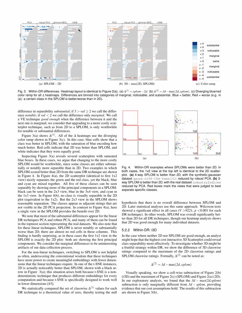
real

gaus

sian

enta

ngle

dgr

id

PCA robust PCA glimmer MDS t-SNEpca - splompca - splompca - splompca - splompca - splompca - splompca - splompca - splompca - splompca - splompca - splompca - splompca - splompca - splompca - splompca - splom robpca - splomrobpca - splomrobpca - splomrobpca - splomrobpca - splomrobpca - splomrobpca - splomrobpca - splomrobpca - splomrobpca - splomrobpca - splomrobpca - splomrobpca - splomrobpca - splomrobpca - splomrobpca - splom glimmer - splomglimmer - splomglimmer - splomglimmer - splomglimmer - splomglimmer - splomglimmer - splomglimmer - splomglimmer - splomglimmer - splomglimmer - splomglimmer - splomglimmer - splomglimmer - splomglimmer - splomglimmer - splom tsne - splomtsne - splomtsne - splomtsne - splomtsne - splomtsne - splomtsne - splomtsne - splomtsne - splomtsne - splomtsne - splomtsne - splomtsne - splomtsne - splomtsne - splomtsne - splom

abalone 0.0 0.0 0.0 0.0 0.0 0.0 0.0 0.0 0.0 0.0 0.0 0.0 0.0 0.0 0.0 0.0 0.0 0.0 0.0 0.0 0.0 0.0 0.0 0.0 0.0 0.0 0.0 0.0 0.0 0.0 0.0 0.0 0.0 0.0 0.0 0.0 0.0 0.0 0.0 0.0 0.0 0.0 0.0 0.0 0.0 0.0 0.0 0.0

cars03Cropped_d2 0.0 0.0 0.0 0.0 0.0 0.0 0.0 0.0 0.0 0.0 0.0 0.0 0.0 0.0 0.0 0.0 0.0 0.0 0.0 0.0 0.0 0.0 0.0 0.0 0.0 0.0 0.0 0.0 0.0 0.0 0.0 0.0 0.0 0.0 0.0 0.0 0.0 0.0 0.0 0.0 0.0 0.0 0.0 0.0 0.0 0.0 0.0 0.0

italianwines 4.0 3.0 1.0 1.0 1.5 3.0 2.5 3.0 3.0 2.5 3.5 4.0 4.0 4.0 3.0 1.0 1.0 2.5 3.0 2.5 3.0 2.5 2.5 3.0 4.0 4.0 -0.5 0.5 1.5 0.0 0.5 0.5 0.0 -0.5 -0.5 0.0 0.5 0.0 1.0 0.5 1.0 1.0 0.5 0.5 -1.0 0.5 0.5 0.0 0.0 0.5 0.5 1.5

worldmap 0.0 0.0 2.0 1.0 0.0 0.0 0.0 2.0 0.0 2.0 1.0 0.0 0.0 0.0 0.0 0.0 2.0 0.0 3.0 1.0 3.0 1.5 0.5 0.0 0.0 1.5 4.0 0.5 0.0 0.0 0.0 0.0 0.0 3.0 0.0 0.0 0.0 0.0 0.0 0.0 0.0 0.0 0.0 0.0 0.0 0.0 0.0 0.0 0.0 0.0 0.0 1.0

cars03Cropped_d3 0.0 0.0 0.0 0.0 0.0 0.5 1.5 0.5 0.5 0.5 0.0 -0.5 0.0 1.5 0.0 0.0 0.5 0.0 2.5 0.0 0.5 2.5 0.0 0.0 0.0 0.0 0.0 0.0 0.0 0.0 0.0 0.0 0.0 -0.5 0.0 0.0

fisheries_clusteredByEscapementTarget 2.5 2.5 2.5 3.0 3.0 3.0 3.0 3.0 3.0 3.0 3.0 0.0 0.0 0.0 0.0 0.0 0.0 0.0 0.0 0.0 0.0 0.0 2.0 1.0 1.5 1.0 0.5 0.0 0.0 0.5 0.5 0.5 0.5 1.5 1.0 1.0 1.0 1.5 2.0 1.0 1.0 2.0 1.5 1.0

fisheries_clusteredByHarvestRule 0.0 0.5 2.0 4.0 4.0 4.0 4.0 4.0 4.0 4.0 4.0 0.0 0.5 2.0 4.0 3.5 4.0 4.0 4.0 4.0 4.0 4.0 0.0 0.0 0.0 0.0 0.0 0.0 0.0 0.0 0.0 0.0 0.0 0.0 0.0 0.0 1.0 0.5 -2.0 -2.0 -2.0 -2.0 -1.0 -1.0

yeast 0.0 0.0 0.0 0.0 0.0 -1.0 -0.5 0.0 0.0 0.0

ecoliproteins 0.0 0.0 0.0 4.0 0.0 3.0 4.0 0.5 0.0 0.5 0.0 1.0 -0.5 2.0 0.0 2.0

efashion 0.0 0.0 0.0 0.0 0.0 0.0 0.0 0.0 0.0 0.0 0.0 0.0 0.0 0.0 0.0 0.0 0.0 0.0 0.0 0.0 -0.5 0.0 0.0 -0.5

tse300 0.0 0.0 -0.5 0.0 0.0 0.5 0.0 0.0 0.0 0.0 0.0 0.0 0.0 1.0 0.0 0.0 -0.5 0.0 0.0 0.0 -0.5 2.0 0.5 0.0 0.0 0.0 0.0 0.0 0.0 0.0 0.0 0.0

cereal 0.0 0.0 0.0 0.0 0.0 0.0 0.0 0.0 0.0 0.0 0.0 0.0 0.0 0.0 0.0 0.0 0.0 0.0 0.0 0.0 0.0

shuttle_big 0.0 0.0 0.0 0.0 0.0 0.0 0.0 0.0 0.0 0.0 -0.5 -0.5 0.0 0.0

shuttle_small 0.5 0.0 0.5 1.0 0.5 0.0 0.0 0.0 0.0 0.0 -1.0 -0.5 -1.0 -0.5

musicnetgroups 0.0 0.0 0.0 0.5 0.0 0.0 0.0 0.0 0.0 0.0 0.0 0.0 0.0 0.0 0.0 0.0 0.5 0.0 0.0 0.0 0.0 3.0 1.0 2.0

hiv 1.0 1.0 0.0 1.0 0.5 0.0 1.0 1.0 0.0 0.0 0.0 0.0

bbdm13 1.0 1.0 2.5 1.5 2.0 0.0 0.0 0.0 0.0 0.0 0.0 0.0 0.0 0.0 0.0

white_ballance 2.0 1.5 0.0 0.0 0.5 0.5 2.0 0.5 2.0 0.5 0.0 0.5 0.5 1.0 0.0

world_11d 0.5 1.5 2.5 0.5 0.5 0.0 0.5 3.0 0.5 2.0 0.0 0.5 1.5 1.5 0.5 1.5 0.5 2.0 0.5 1.5

world_9d 1.0 1.5 3.0 0.0 1.5 0.0 0.5 -0.5 -0.5 0.5 2.0 2.0 1.0 0.5 3.0

boston 1.0 2.5 3.5 0.0 0.0 0.0 0.0 1.0 0.5 -0.5 1.0 0.5

iris 0.0 0.0 0.0 0.0 0.0 0.0 0.0 0.5 0.5 0.0 1.0 0.5

olive 0.0 0.0 0.0 0.0 0.0 0.0 0.0 0.0 0.0 0.0 0.0 0.0

swanson 0.0 0.0 0.0 0.0 0.0 0.0 0.0 0.0 0.0

wine 0.5 1.5 1.5 0.0 2.0 2.0 0.0 0.0 0.5 0.5 1.0 1.5

breast-cancer-wisconsin 0.0 0.0 0.0 0.0 1.0 1.5

cars03Cropped_d1 1.0 1.0 0.0 0.0 0.5 0.5

ionosphere 1.0 1.5 0.0 0.0

parkinsons_abs_croped 0.0 -0.5 0.5 0.0 0.0 -0.5

spambase 2.0 1.5 0.5 0.5

wdbc_class_1_2 1.0 1.0 0.0 0.0 0.0 0.0 1.0 1.0

n100-d10-c5-spr0.1-out0 1.0 0.0 0.0 0.0 0.5 4.0 0.0 3.5 0.0 3.5 2.5 1.0 3.0 1.0 2.0 1.0 0.0 0.5 0.0 0.5

n100-d10-c5-spr0.2-out0 0.5 0.0 1.5 0.0 1.5 -0.5 -0.5 1.5 0.0 2.0 0.5 0.5 1.5 0.5 1.5 0.5 1.0 2.0 2.0 1.5

n100-d5-c5-spr0.1-out0 0.0 0.0 0.0 0.0 0.0 0.0 0.0 0.0 0.0 0.0 0.0 0.5 0.0 -0.5 0.0 0.5 1.5 0.5 1.0 0.5

n100-d5-c5-spr0.2-out0 0.0 0.0 0.0 0.0 0.0 0.0 0.5 1.0 0.5 0.0 0.0 0.0 0.0 0.0 -1.0 0.0 0.5 0.0 1.0 0.5

n500-d10-c5-spr0.1-out0 0.0 1.5 1.5 1.0 0.0 0.0 1.5 1.5 0.5 0.0 0.5 0.5 0.5 0.0 0.0 0.0 -0.5 -1.0 0.0 0.0

n500-d10-c5-spr0.2-out0 0.0 0.5 1.0 2.0 0.0 0.5 0.0 1.0 2.5 0.0 0.0 1.0 0.5 1.0 0.5 1.0 0.5 0.0 0.0 -0.5

n500-d5-c5-spr0.1-out0 0.0 0.0 0.5 0.0 0.5 0.0 0.0 0.5 0.0 0.5 0.0 0.5 0.0 1.0 0.0 0.0 0.5 0.0 0.5 1.0

n500-d5-c5-spr0.2-out0 0.0 0.0 1.0 0.0 0.0 -0.5 0.0 0.5 0.0 0.5 0.0 0.5 0.5 1.0 1.5 0.5 1.0 1.0 0.5 1.5

n100-d10-c3-spr0.1-out0 0.0 0.0 0.0 0.0 0.0 0.0 0.0 0.5 0.0 1.5 1.0 0.0

n100-d10-c3-spr0.2-out0 0.0 0.0 0.0 0.5 0.0 0.0 0.5 0.5 1.5 2.0 1.0 1.0

n100-d5-c3-spr0.1-out0 0.0 0.0 0.0 0.0 0.5 0.0 0.0 0.0 0.0 0.0 1.0 0.5

n100-d5-c3-spr0.2-out0 0.5 0.0 0.0 1.0 0.0 0.0 1.5 1.5 1.5 0.5 0.5 1.0

n500-d10-c3-spr0.1-out0 0.0 0.0 0.0 0.0 0.0 0.0 0.0 0.0 0.0 0.0 0.0 0.0

n500-d10-c3-spr0.2-out0 0.0 0.0 0.0 0.0 0.0 0.0 0.5 0.5 0.5 0.0 0.5 -0.5

n500-d5-c3-spr0.1-out0 0.0 0.0 0.0 0.0 0.0 0.0 0.0 0.0 0.0 0.0 0.0 0.0

n500-d5-c3-spr0.2-out0 0.0 0.0 0.0 0.0 0.0 0.0 0.0 0.0 0.0 0.0 0.0 0.0

interleaved_100_200_15d_0_notcramped_notrotated 1.0 1.0 1.5 2.0 0.5 0.0 2.0 1.5 1.5 0.5 3.0 3.0 -0.5 1.0 0.0 1.0 0.5 1.0 2.5 0.0 0.0 2.5 1.5 1.5 0.5 3.0 2.5 -0.5 1.0 0.0 1.0 1.5 1.0 0.5 1.5 1.5 2.0 2.5 1.5 1.0 1.5 0.5 1.5 1.0 2.0 0.0 0.0 0.0 0.0 0.0 0.0 0.0 0.0 0.0 0.0 0.0 0.0 0.0 0.0 0.0

interleaved_100_200_15d_25_cramped_rotated 0.0 0.5 1.0 0.0 3.5 1.5 1.5 2.0 1.0 1.0 0.5 1.0 -0.5 -0.5 0.0 0.0 0.5 1.0 0.0 3.5 2.0 1.5 1.5 1.0 0.5 0.5 0.5 -0.5 -0.5 0.0 1.0 1.5 0.5 1.5 2.5 1.0 2.5 2.5 1.0 1.5 1.0 0.5 1.0 0.0 1.0 0.0 0.0 0.0 0.0 0.0 0.5 0.0 0.0 0.0 0.0 0.0 0.0 0.0 0.0 0.0

interleaved_100_200_10d_0_notcramped_notrotated 0.0 0.0 0.0 0.0 4.0 4.0 0.0 0.0 2.0 1.5 0.5 -0.5 0.0 0.0 4.0 3.5 0.0 0.0 1.0 1.5 1.0 0.0 1.0 0.0 2.5 1.5 1.5 0.5 1.0 2.0 0.0 -0.5 -0.5 0.0 0.0 0.0 -1.0 0.0 0.0 0.0

interleaved_100_200_10d_25_cramped_rotated 1.0 0.0 3.0 2.5 2.0 -0.5 0.5 -0.5 0.5 2.0 1.0 0.5 3.0 2.0 2.5 -1.0 0.5 -0.5 0.0 2.0 2.0 0.5 1.5 1.5 2.5 1.5 2.0 1.5 2.0 1.0 0.0 -1.0 0.0 0.0 0.0 0.0 0.0 0.0 0.0 0.0

interleaved_100_200_6d_0_notcramped_notrotated 1.0 1.5 1.5 0.0 1.0 0.0 1.0 0.5 1.0 0.0 0.0 0.0 1.5 0.5 0.5 1.0 1.0 -0.5 0.0 0.0 0.0 0.5 0.5 0.0

interleaved_100_200_6d_25_cramped_rotated 0.0 0.5 0.0 0.0 0.0 1.0 0.0 0.5 0.0 0.0 0.0 1.0 -0.5 0.5 0.0 -0.5 0.0 1.0 0.5 0.0 0.5 0.0 0.0 0.5

interleaved_100_200_5d_0_notcramped_notrotated 0.0 0.0 1.0 0.5 0.5 0.5 0.0 0.5 0.5 0.5 0.0 2.0 0.5 1.5 0.5 0.0 0.0 0.0 0.0 0.0

interleaved_100_200_5d_25_cramped_rotated 0.0 1.5 0.5 -0.5 -0.5 0.0 1.5 0.0 0.0 0.0 0.5 2.0 0.0 0.5 2.0 0.0 0.0 0.5 0.0 0.0

JavierGeneratedData_3dinterleaved_5classes 0.5 0.5 0.0 1.0 0.0 0.0 0.0 1.0 0.5 1.0 0.5 1.0 0.0 0.5 -0.5 0.5 0.0 0.0 0.0 0.0

interleaved_100_200_4d_0_notcramped_notrotated 0.0 0.5 0.0 0.5 0.0 0.5 0.0 0.5 -0.5 1.0 0.0 1.5 0.0 0.0 0.0 1.0

interleaved_100_200_4d_25_cramped_rotated 2.5 0.5 1.0 0.0 2.5 0.5 1.0 0.0 0.5 0.0 1.0 0.5 0.5 0.0 0.5 0.0

JavierGeneratedData_3dinterleaved_4classes 0.0 0.0 0.0 0.0 0.0 0.5 0.0 0.0 0.0 0.0 -1.0 0.0 0.0 0.0 0.0 0.0

interleaved_100_500_3_25_cramped_rotated 0.0 0.0 0.0 0.0 0.0 0.0 0.0 0.0 -0.5 0.0 0.0 0.5

interleaved_250_500_3_0_notCramped_rotated 0.0 0.0 0.0 0.0 0.0 0.0 -0.5 -0.5 -0.5 0.0 -0.5 0.5

JavierGeneratedData_3dinterleaved_3classes 0.0 0.0 0.0 0.0 0.0 0.0 0.0 -0.5 -0.5 0.0 0.0 0.0

ms_interleaved_120_240_3d_25_centeredClusters -0.5 -0.5 -0.5 -0.5 -0.5 -0.5 -0.5 0.0 0.0 0.5 1.5 0.5

ms_interleaved_120_240_3d_50_centeredClusters 0.0 0.0 0.0 0.0 0.0 0.0 0.0 0.0 0.0 0.0 0.0 0.0

ms_interleaved_40_80_3d_0 0.0 0.0 0.0 0.0 0.0 0.0 -0.5 -0.5 -0.5 1.5 1.5 0.5

ms_interleaved_40_80_3d_50 0.0 0.0 0.0 0.0 0.0 0.0 -0.5 -0.5 -0.5 0.0 0.0 0.0

ms_interleaved_400_800_3d_0 0.0 0.0 0.0 0.0 0.0 0.0 -0.5 -0.5 -0.5 0.0 0.0 1.0

ms_interleaved_400_800_3d_50 0.0 0.0 0.0 0.0 0.0 0.0 -0.5 0.0 0.0 0.0 0.0 0.0




grid6_4d 0.0 0.0 0.0 0.0 0.0 0.0 0.0 0.0 0.0 0.0 0.0 0.0 0.0 0.0 0.0 0.0 0.5 0.0 0.0 4.0 0.0 0.0 0.0 4.0 4.0 4.0 0.0 0.0 0.0 -4.0 0.0 0.0 1.0 0.0 1.5 1.0 0.5 1.5 1.0 0.5 0.5 0.5 0.0 0.5 0.5 1.5 1.0 1.5 -1.0 0.5 0.5 0.0 1.0 1.5 -1.0 -1.0 0.0 -1.0 -0.5 0.0 -1.0 -1.0 -1.5 -1.0

grid10_3d 0.5 0.5 0.5 0.5 0.0 0.0 0.0 0.0 0.0 0.0 0.5 3.0 3.0 0.5 0.0 0.0 1.5 0.5 1.0 1.5 1.5 1.0 1.0 1.5 1.0 -1.5 1.5 -0.5 1.0 -1.5 0.5 -1.0

twosquare-nome 4.0 3.0 0.0 0.0 4.0 3.0 0.0 0.0 3.5 3.5 3.5 3.5 0.0 0.0 0.0 0.0

UnEvenDensity-nome 0.0 0.0 0.0 0.0 0.5 -0.5

(a) SPLOM – 2D

PCA robust PCA glimmer MDS t-SNEpca - 3Dpca - 3Dpca - 3Dpca - 3Dpca - 3Dpca - 3Dpca - 3Dpca - 3Dpca - 3Dpca - 3Dpca - 3Dpca - 3Dpca - 3Dpca - 3Dpca - 3Dpca - 3D robpca - 3Drobpca - 3Drobpca - 3Drobpca - 3Drobpca - 3Drobpca - 3Drobpca - 3Drobpca - 3Drobpca - 3Drobpca - 3Drobpca - 3Drobpca - 3Drobpca - 3Drobpca - 3Drobpca - 3Drobpca - 3D glimmer - 3Dglimmer - 3Dglimmer - 3Dglimmer - 3Dglimmer - 3Dglimmer - 3Dglimmer - 3Dglimmer - 3Dglimmer - 3Dglimmer - 3Dglimmer - 3Dglimmer - 3Dglimmer - 3Dglimmer - 3Dglimmer - 3Dglimmer - 3D tsne - 3Dtsne - 3Dtsne - 3Dtsne - 3Dtsne - 3Dtsne - 3Dtsne - 3Dtsne - 3Dtsne - 3Dtsne - 3Dtsne - 3Dtsne - 3Dtsne - 3Dtsne - 3Dtsne - 3Dtsne - 3D

abalone 0.0 0.0 0.0 0.0 0.0 0.0 0.0 0.0 0.0 0.0 0.0 0.0 0.0 0.0 0.0 0.0 0.0 0.0 0.0 0.0 0.0 0.0 0.0 0.0 0.0 0.0 0.0 0.0 0.0 0.0 0.0 0.0 0.0 0.0 0.0 0.0 0.0 0.0 0.0 0.0 0.0 0.0 0.0 0.0 0.0 0.0 0.0 0.0

cars03Cropped_d2 0.0 0.0 0.0 0.0 0.0 0.0 0.0 0.0 0.0 0.0 0.0 0.0 0.0 0.0 0.0 0.0 0.0 0.0 0.0 0.0 0.0 0.0 0.0 0.0 0.0 0.0 0.0 0.0 0.0 0.0 0.0 0.0 0.0 0.0 0.0 0.0 0.0 0.0 0.0 0.0 0.0 0.0 0.0 0.0 0.0 0.0 0.0 0.0

italianwines -2.0 -1.0 1.0 1.0 0.5 -1.0 -0.5 -1.0 -1.0 -0.5 -0.5 -0.5 -0.5 -2.5 -1.5 0.5 0.5 -1.0 -1.5 -1.0 -1.5 -1.0 -1.0 -0.5 -0.5 -0.5 -0.5 0.5 0.5 -0.5 -0.5 0.0 0.5 -1.0 -1.0 0.0 0.0 0.5 -0.5 -0.5 0.0 -1.0 -0.5 -0.5 -1.0 -0.5 -0.5 0.0 0.0 -1.0 -0.5 0.0

worldmap 0.0 0.0 0.0 0.0 0.0 0.0 0.0 0.0 0.0 0.5 0.0 0.0 0.0 0.0 0.0 0.0 0.0 0.0 0.0 0.0 0.0 0.0 0.0 0.0 0.0 0.5 0.0 0.0 0.0 0.0 0.0 0.0 0.0 0.0 0.0 0.0 0.0 0.0 0.0 0.0 0.0 0.0 0.0 0.0 0.0 0.0 0.0 0.0 -0.5 -1.0 0.0 -0.5

cars03Cropped_d3 1.0 -1.0 0.5 -1.0 0.0 -0.5 -1.5 0.0 -1.0 0.0 0.0 -1.5 0.5 -1.0 0.0 0.0 -0.5 0.0 -2.0 0.0 -0.5 -2.5 0.0 0.0 0.5 0.0 0.0 0.5 0.0 0.0 1.5 0.5 0.0 1.0 0.0 1.5

fisheries_clusteredByEscapementTarget -1.0 -1.0 -1.0 -1.5 -1.5 -1.5 -2.0 -2.0 -2.0 -2.0 -2.0 0.0 0.0 0.0 0.0 0.0 0.0 0.0 0.0 0.0 0.0 0.0 -0.5 0.0 -0.5 0.0 0.0 0.0 0.0 -0.5 -0.5 -0.5 -0.5 -1.0 -0.5 -0.5 -1.0 -1.5 -0.5 -0.5 -1.0 -1.0 -0.5 -0.5

fisheries_clusteredByHarvestRule 0.0 -0.5 -0.5 -0.5 -0.5 -0.5 -1.0 -2.0 -2.0 -2.0 -2.0 0.0 0.0 0.0 0.0 0.5 0.0 -0.5 -1.0 -2.0 -2.0 -2.0 0.0 0.0 0.0 0.0 0.0 0.0 0.0 0.0 0.0 0.0 0.0 0.0 0.0 0.0 0.0 0.5 1.0 1.0 1.0 1.0 1.5 1.5

yeast 0.0 0.5 1.0 0.0 0.0 0.0 0.5 0.0 0.0 0.0

ecoliproteins 0.0 1.0 0.0 -4.0 0.5 -3.0 -3.5 0.5 -1.0 -1.5 0.0 -1.0 0.0 -0.5 -0.5 -0.5

efashion 0.0 0.0 0.0 0.0 0.0 0.0 0.0 0.0 0.0 0.0 0.0 0.0 1.0 0.0 0.0 0.5 0.0 0.0 0.0 0.0 0.0 0.0 0.0 0.0

tse300 0.0 -0.5 0.0 -0.5 0.5 1.5 0.0 0.0 0.0 -0.5 0.5 -0.5 0.5 1.0 0.0 0.0 -0.5 0.0 0.0 0.0 -0.5 -1.0 0.0 0.0 0.0 0.0 0.0 0.0 0.0 0.0 0.0 0.0

cereal 0.0 0.0 0.0 0.0 0.0 0.0 0.0 0.0 0.0 0.0 0.0 0.0 0.0 0.0 0.0 0.0 0.0 0.0 0.0 0.0 0.0

shuttle_big 0.0 0.0 0.0 0.0 0.0 -0.5 -0.5 0.0 0.0 0.0 -0.5 -0.5 0.0 0.0

shuttle_small -0.5 0.0 0.0 0.0 0.5 0.0 0.0 0.0 0.0 0.0 -1.0 -0.5 -1.0 -0.5

musicnetgroups 0.0 0.0 0.0 0.0 0.0 0.0 0.0 0.0 0.0 0.0 0.0 0.0 0.0 0.0 0.0 1.0 0.5 0.0 0.0 0.0 0.0 -1.5 -1.0 -2.0

hiv -0.5 0.5 0.0 -1.0 -0.5 0.0 -1.0 -0.5 -1.0 -1.0 0.0 0.0

bbdm13 0.0 0.5 0.5 0.5 0.0 0.0 0.0 0.0 0.0 0.0 -0.5 0.0 0.0 0.0 0.0

white_ballance -1.0 -1.5 -0.5 -0.5 -0.5 -0.5 -2.0 -1.0 -2.0 -0.5 1.0 -0.5 -1.0 0.5 0.0

world_11d -0.5 -0.5 -1.5 -0.5 -0.5 0.5 -0.5 -1.0 0.0 -0.5 0.0 0.0 0.0 -1.0 0.0 0.0 0.0 0.0 -0.5 0.5

world_9d 0.0 0.0 -3.0 0.0 -1.0 0.0 0.0 0.0 0.5 -0.5 -1.0 -1.0 -1.0 0.0 0.5

boston -0.5 -1.5 -2.5 0.5 0.5 0.5 0.5 0.0 0.0 -0.5 0.0 -0.5

iris 0.0 0.0 0.0 0.0 0.5 0.5 0.0 0.0 0.0 0.0 -0.5 -0.5

olive 0.5 0.0 0.5 0.0 0.0 0.5 0.5 0.0 0.5 0.0 0.0 -0.5

swanson 0.0 0.0 -1.0 0.0 0.0 0.0 0.0 0.0 -1.5

wine -0.5 -1.5 -1.5 0.0 -1.5 -1.5 0.5 0.5 0.0 -1.0 -0.5 -1.5

breast-cancer-wisconsin 0.0 0.0 0.0 -0.5 -0.5 -0.5

cars03Cropped_d1 1.0 1.0 -0.5 0.0 0.5 0.5

ionosphere 0.5 0.0 0.0 0.0

parkinsons_abs_croped 0.0 0.0 -0.5 -0.5 0.0 -0.5

spambase -2.0 -2.0 0.0 0.0

wdbc_class_1_2 -1.0 -0.5 0.0 0.0 0.0 0.0 -1.5 0.0

n100-d10-c5-spr0.1-out0 0.0 0.0 0.0 0.0 0.5 0.0 0.0 0.0 0.0 -0.5 0.0 0.5 -0.5 0.5 1.0 0.0 -0.5 -0.5 1.0 0.5

n100-d10-c5-spr0.2-out0 -1.5 -1.0 -1.0 0.0 0.0 0.0 -2.0 -1.5 -1.0 0.0 -0.5 -1.0 -1.0 -1.0 -1.5 0.0 -0.5 -1.5 -1.5 -1.0

n100-d5-c5-spr0.1-out0 -0.5 0.5 0.0 -0.5 0.5 -0.5 0.0 -0.5 -0.5 0.5 0.0 1.0 -0.5 0.0 -0.5 -0.5 -1.5 -0.5 -0.5 1.0

n100-d5-c5-spr0.2-out0 0.0 0.0 0.0 0.0 -1.0 0.5 0.5 0.0 0.0 0.0 -0.5 -0.5 0.5 -0.5 -1.5 0.5 0.5 1.0 0.0 0.5

n500-d10-c5-spr0.1-out0 0.0 -1.0 -0.5 -0.5 -0.5 0.0 -1.5 -1.0 -0.5 -1.0 0.0 2.0 1.5 0.5 -0.5 0.0 0.5 0.5 0.5 0.0

n500-d10-c5-spr0.2-out0 1.5 0.0 1.5 1.0 0.5 1.5 0.5 1.0 0.5 0.5 0.0 -1.0 -0.5 -1.0 -0.5 -0.5 0.5 0.5 0.0 0.5

n500-d5-c5-spr0.1-out0 0.5 0.5 0.5 0.5 0.5 0.5 1.0 0.5 1.0 0.5 0.5 1.0 1.5 -0.5 0.5 0.0 -0.5 0.0 0.0 -0.5

n500-d5-c5-spr0.2-out0 0.5 0.5 0.0 1.0 0.5 0.0 1.0 0.0 0.0 0.0 0.5 0.5 0.0 -0.5 -0.5 0.0 -1.0 -0.5 0.0 -1.0

n100-d10-c3-spr0.1-out0 0.0 0.0 0.0 0.0 0.0 0.0 0.0 0.0 0.0 0.0 0.5 0.5

n100-d10-c3-spr0.2-out0 0.5 0.0 0.5 0.0 0.0 0.5 -0.5 -0.5 -1.0 -0.5 -0.5 -0.5

n100-d5-c3-spr0.1-out0 0.0 0.0 0.0 0.0 0.0 0.0 0.0 0.0 0.0 0.0 0.0 0.0

n100-d5-c3-spr0.2-out0 0.0 0.0 0.0 0.5 0.5 0.0 0.5 1.0 0.5 -1.5 -1.0 -1.0

n500-d10-c3-spr0.1-out0 0.0 0.0 0.0 0.0 0.0 0.0 0.0 0.0 0.0 0.0 0.0 0.0

n500-d10-c3-spr0.2-out0 0.0 0.5 0.0 0.0 0.5 0.0 -0.5 0.0 -0.5 0.0 -0.5 -1.0

n500-d5-c3-spr0.1-out0 0.0 0.0 0.0 0.0 0.0 0.0 0.0 0.5 0.5 0.0 0.0 0.0

n500-d5-c3-spr0.2-out0 -0.5 0.5 0.5 0.0 0.5 0.0 0.5 0.5 0.5 0.0 0.0 0.0

interleaved_100_200_15d_0_notcramped_notrotated 1.0 1.5 2.5 -0.5 -0.5 1.5 0.5 1.0 0.0 0.5 -2.0 0.0 1.0 0.5 1.0 1.5 2.0 3.0 -0.5 0.5 1.0 -0.5 1.0 -0.5 0.5 -2.0 0.0 0.0 1.5 0.5 0.5 -1.0 0.0 0.0 -1.0 -1.0 -2.0 -2.0 -1.0 0.0 -0.5 0.0 -0.5 -0.5 -0.5 0.0 0.0 0.0 0.0 0.0 0.0 0.0 0.0 0.0 0.0 0.0 0.0 0.0 0.0 0.0

interleaved_100_200_15d_25_cramped_rotated 1.5 1.0 0.5 1.0 -2.0 0.5 0.0 1.5 -0.5 0.5 -0.5 0.5 0.5 1.0 0.5 2.0 0.5 0.5 1.5 -1.5 0.0 0.0 1.5 -0.5 1.0 -0.5 1.5 1.0 1.0 0.5 -1.0 -1.5 -0.5 -1.5 -2.5 -1.0 -2.5 -2.5 -1.0 -1.5 -1.0 -0.5 -1.0 0.0 -1.0 0.0 0.0 0.0 0.0 0.0 0.0 0.0 0.0 0.0 0.0 0.0 0.0 0.0 0.5 0.0

interleaved_100_200_10d_0_notcramped_notrotated 0.5 0.0 0.5 0.0 -0.5 -2.0 0.5 0.5 -1.5 0.0 0.5 0.0 0.5 0.0 -0.5 -2.0 -0.5 0.5 -0.5 0.0 0.0 0.5 0.5 1.0 -2.0 -1.0 -1.0 0.5 -0.5 -1.5 0.0 0.0 0.0 0.0 0.0 0.0 0.0 0.0 0.0 0.0

interleaved_100_200_10d_25_cramped_rotated 0.5 1.0 0.0 -1.5 0.5 1.0 0.5 1.0 0.0 -1.0 1.0 0.5 0.0 -1.0 0.5 1.0 0.5 1.0 0.0 -1.0 0.5 2.0 0.5 1.0 0.0 1.0 0.0 1.0 0.5 1.5 0.0 0.0 0.0 0.0 0.0 0.0 0.0 0.0 0.0 0.0

interleaved_100_200_6d_0_notcramped_notrotated 0.5 1.0 0.0 0.5 0.5 0.5 0.5 1.0 0.5 1.0 1.0 0.5 1.0 0.5 0.5 0.5 0.0 0.0 0.0 0.5 -0.5 -0.5 0.0 0.5

interleaved_100_200_6d_25_cramped_rotated 0.0 0.5 1.5 0.0 0.0 1.0 0.0 0.5 1.5 0.0 0.0 0.5 0.5 0.5 1.5 1.0 0.5 0.5 0.0 0.0 0.5 0.0 0.0 0.0

interleaved_100_200_5d_0_notcramped_notrotated 2.5 2.0 0.5 1.0 0.5 2.0 1.5 1.0 1.0 0.5 0.5 1.5 0.5 0.5 1.0 0.0 0.0 0.0 0.0 0.0

interleaved_100_200_5d_25_cramped_rotated 1.5 0.5 1.0 1.0 1.0 2.0 0.5 1.0 1.0 1.0 1.0 0.0 1.0 0.5 1.0 0.5 0.5 -0.5 0.5 0.0

JavierGeneratedData_3dinterleaved_5classes 0.5 0.5 0.0 0.0 0.0 0.5 0.5 0.0 0.0 0.0 0.5 0.0 0.0 0.5 0.0 0.0 0.0 0.0 0.0 0.0

interleaved_100_200_4d_0_notcramped_notrotated 1.0 0.5 1.0 1.0 1.0 0.5 1.0 1.0 1.5 1.0 1.5 1.5 0.0 0.0 0.0 0.0

interleaved_100_200_4d_25_cramped_rotated 1.0 1.0 1.5 0.5 1.0 1.0 1.5 0.5 0.5 0.5 1.0 0.5 0.5 0.5 0.0 0.0

JavierGeneratedData_3dinterleaved_4classes 0.5 0.5 0.0 0.5 0.5 0.5 0.5 1.0 0.0 0.0 0.0 0.0 0.0 0.0 0.0 0.0

interleaved_100_500_3_25_cramped_rotated 0.0 0.0 0.0 0.0 0.0 0.0 0.0 0.0 0.0 -0.5 -0.5 -1.0

interleaved_250_500_3_0_notCramped_rotated 0.0 0.0 0.0 0.0 0.0 0.0 0.0 0.0 0.0 0.5 0.0 0.5

JavierGeneratedData_3dinterleaved_3classes 0.5 0.5 0.5 0.5 0.5 0.5 0.0 0.0 0.0 0.0 0.0 0.0

ms_interleaved_120_240_3d_25_centeredClusters 0.0 0.0 0.0 0.0 0.0 0.0 0.5 0.5 0.5 0.0 -0.5 0.0


ms_interleaved_40_80_3d_0 0.0 0.0 0.0 0.0 0.0 0.0 0.0 0.0 0.0 0.0 0.0 0.0

ms_interleaved_40_80_3d_50 0.0 0.0 0.0 0.5 0.5 0.5 0.0 0.0 0.0 0.0 0.0 0.0

ms_interleaved_400_800_3d_0 0.0 0.0 0.0 0.0 0.0 0.0 0.0 0.0 0.0 0.0 0.0 -0.5

ms_interleaved_400_800_3d_50 0.5 0.5 0.5 0.5 0.5 0.5 0.0 0.0 0.0 0.0 0.0 0.0



ms_interleaved_60_120_3d_50_centeredClusters 0.5 0.5 0.5 0.5 0.5 0.5 -0.5 -0.5 -0.5 1.0 1.0 1.0

grid6_4d 0.0 0.0 0.0 0.0 0.0 0.0 0.0 0.0 0.0 0.0 0.0 0.0 0.0 0.0 0.0 0.0 0.5 1.0 1.0 -3.0 -3.0 -3.0 -3.0 -3.0 -3.0 -3.0 1.0 1.0 -3.0 -3.0 -3.0 -3.0 -0.5 0.5 -1.0 -0.5 0.0 -1.0 -0.5 0.0 0.0 0.0 0.5 0.0 0.0 -1.0 -0.5 -1.0 -1.5 -1.0 -1.0 -1.5 -1.5 -1.5 -2.0 -2.0 -1.0 -2.0 -1.5 -1.0 -2.0 -2.0 -2.0 -1.5

grid10_3d 3.0 3.0 3.0 3.0 -0.5 -0.5 -0.5 -0.5 0.5 0.5 0.0 0.0 0.0 0.0 0.5 0.5 0.5 1.5 0.5 0.5 0.5 0.5 1.0 0.5 0.0 -0.5 0.0 0.0 0.0 -0.5 0.5 -1.0

twosquare-nome 0.0 0.0 0.0 0.0 0.0 0.0 0.0 0.0 0.5 0.5 0.5 0.5 0.5 0.5 0.5 0.5

UnEvenDensity-nome 0.0 0.0 0.0 0.0 0.0 -0.5

(b) 3D – max(2D, SPLOM)

ID

123456789

101112131415161718192021222324252627282930313233343536373839404142434445464748495051525354555657585960616263646566676869707172737475

1 abalone17 bbdm1321 boston26 breast-cancer-wisconsin27 cars03Cropped_d12 cars03Cropped_d25 cars03Cropped_d3

12 cereal9 ecoliproteins

10 efashion6 fisheries_clusteredByEscapementTarget7 fisheries_clusteredByHarvestRule

73 grid10_3d72 grid6_4d16 hiv50 interleaved_100_200_10d_0_notcramped_notrotated51 interleaved_100_200_10d_25_cramped_rotated48 interleaved_100_200_15d_0_notcramped_notrotated49 interleaved_100_200_15d_25_cramped_rotated57 interleaved_100_200_4d_0_notcramped_notrotated58 interleaved_100_200_4d_25_cramped_rotated54 interleaved_100_200_5d_0_notcramped_notrotated55 interleaved_100_200_5d_25_cramped_rotated52 interleaved_100_200_6d_0_notcramped_notrotated53 interleaved_100_200_6d_25_cramped_rotated60 interleaved_100_500_3_25_cramped_rotated61 interleaved_250_500_3_0_notCramped_rotated28 ionosphere22 iris3 italianwines

62 JavierGeneratedData_3dinterleaved_3classes59 JavierGeneratedData_3dinterleaved_4classes56 JavierGeneratedData_3dinterleaved_5classes63 ms_interleaved_120_240_3d_25_centeredClusters64 ms_interleaved_120_240_3d_50_centeredClusters65 ms_interleaved_40_80_3d_066 ms_interleaved_40_80_3d_5067 ms_interleaved_400_800_3d_068 ms_interleaved_400_800_3d_5069 ms_interleaved_60_120_3d_0_centeredClusters70 ms_interleaved_60_120_3d_25_centeredClusters71 ms_interleaved_60_120_3d_50_centeredClusters15 musicnetgroups40 n100-d10-c3-spr0.1-out041 n100-d10-c3-spr0.2-out032 n100-d10-c5-spr0.1-out033 n100-d10-c5-spr0.2-out042 n100-d5-c3-spr0.1-out043 n100-d5-c3-spr0.2-out034 n100-d5-c5-spr0.1-out035 n100-d5-c5-spr0.2-out044 n500-d10-c3-spr0.1-out045 n500-d10-c3-spr0.2-out036 n500-d10-c5-spr0.1-out037 n500-d10-c5-spr0.2-out046 n500-d5-c3-spr0.1-out047 n500-d5-c3-spr0.2-out038 n500-d5-c5-spr0.1-out039 n500-d5-c5-spr0.2-out023 olive29 parkinsons_abs_croped13 shuttle_big14 shuttle_small30 spambase24 swanson11 tse30074 twosquare-nome75 UnEvenDensity-nome31 wdbc_class_1_218 white_ballance25 wine19 world_11d20 world_9d4 worldmap8 yeast

4.0 4 4substantially3.0 < 4 3 / 3.5 substantially

2.0 < 3 2 / 2.5 noticeable1.0 < 2 1 / 1.5

marginal0.5 < 1 0.5 marginal0.0 0 same-0.5 > -1 -0.5

marginal-1.0 > -2 -1 / -1.5 marginal-2.0 > -3 -2 / -2.5 noticeable-3.0 > -4 -3 / -3.5

substantially-4.0 -4 -4 substantially

4.0 = 4 substantial3.0 < 4 substantial2.0 < 3 noticeable1.0 < 2 marginal0.5 < 1 marginal0.0 = 0 same-0.5 > -1 marginal-1.0 > -2 marginal-2.0 > -3 noticeable-3.0 > -4 substantial-4.0 = -4 substantial

(c) Color ramp

Fig. 3. Within-DR differences. Heatmap layout is identical to Figure 2(a). (a) ∆(1) = splom−2d. (b) ∆(2) = 3d−max(2d,splom). (c) Diverging blue/redcolor ramp for all ∆ heatmaps. Differences are binned into categories of marginal, noticeable, and substantial. Blue = better, Red = worse (e.g. in(a): a certain class in the SPLOM is better/worse than in 2D).

difference in separability substantial; if 3 > val ≥ 2 we call the differ-ence notable; if val < 2 we call the difference only marginal. We calla VE technique good enough when the difference between it and thenext one is marginal; we consider that upgrading to a more costly scat-terplot technique, such as from 2D to a SPLOM, is only worthwhilefor notable or substantial differences.

Figure 3(a) shows ∆(1). All of the ∆ heatmaps use the divergingcolor ramp shown in Figure 3(c). In this case, blue cells show that aclass was better in SPLOM, with the saturation of blue encoding howmuch better. Red cells indicate that 2D was better than SPLOM, andwhite indicates that they were equally good.

Inspecting Figure 3(a) reveals several scatterplots with saturatedblue boxes. In these cases, we argue that changing to the more costlySPLOM would be worthwhile, since some classes are either substan-tially or notably more separable than in 2D. Two examples in whichSPLOM scored better than 2D from the same DR technique are shownin Figure 4. In Figure 4(a), the 2D scatterplot (identical to first 1x2view) nicely separates the green and the red class, yet the black, blueand cyan are mixed together. All five of these classes can be seenseparably by showing more of the principal components in a SPLOM:black can be seen in the 2x3 view, blue in the 3x4 view, and cyan inthe 1x3 view. In Figure 4(b), no class is visually separable in the 2Dplot (equivalent to the 1x2). But the 2x3 view in the SPLOM showsreasonable separation. The classes appear as adjacent strings that arenot visible in the 2D PCA projection. In contrast to Figure 4(a), herea single view in the SPLOM provides the benefit over 2D.

We note that most of the substantial differences appear for the linearDR techniques PCA and robust PCA, and many of them can be foundin the topmost section representing the real datasets. We also note thatfor these linear techniques, SPLOM is never notably or substantiallyworse than 2D; there are almost no red cells in these columns. Thisfinding is hardly surprising, as in these cases the first 1x2 view in theSPLOM is exactly the 2D plot: both are showing the first principalcomponents. We consider the marginal differences to be uninterestingartifacts of our data collection process.

For the non-linear techniques, switching to SPLOM is not helpfulas often, underscoring the conventional wisdom that these techniqueshave more power to create meaningful embeddings with fewer dimen-sions that the linear techniques require. In one of the t-SNE instances,2D is actually noticeably better than SPLOM, shown with a black ar-row in Figure 3(a); this situation arises both because t-SNE is a non-deterministic technique that produces different embeddings for everycomputation and because t-SNE is specifically designed to work wellin lower dimensions [43].

We statistically compared the set of classwise ∆(1) values for eachDR technique to a theoretical value of zero, thereby testing the null

−1.0 −0.5 0.0 0.5 1.0

−0.5

0.0

0.5

.x

.y

1x2−1.0 −0.5 0.0 0.5 1.0

−1.0

−0.5

0.0

0.5

.x

.y

−1.0 −0.5 0.0 0.5 1.0

−1.0

−0.5

0.0

0.5

1.0

.x

.y

−1.0 −0.5 0.0 0.5

−1.0

−0.5

0.0

0.5

1.0

.x

.y

−1.0 −0.5 0.0 0.5

−0.5

0.0

0.5

.x

.y

−1.0 −0.5 0.0 0.5 1.0

−0.5

0.0

0.5

.x

.y

1x4

1x3 2x3

2x4 3x4

(a)

1x2

1x3 2x3

(b)

Fig. 4. Within-DR examples where SPLOMs were better than 2D. Inboth cases, the 1x2 view at the top left is identical to the 2D scatter-plot. (a) 4-way SPLOM is better than 2D, with the synthetic-gaussiandataset gauss-n100-10d-5smallCl reduced by robust PCA. (b) 3-way SPLOM is better than 2D, with the real dataset industryIndicesreduced by PCA. Red boxes mark the views that were judged to bestseparate specific classes.

hypothesis that there is no overall difference between SPLOM and2D. Later statistical analyses use this same approach. Wilcoxon testsshowed a significant effect in all cases (V >9221, p <0.001 for eachDR technique). In other words, SPLOM was overall significantly bet-ter than 2D for all DR techniques, though our heatmap analysis showsthat 2D was good enough for many individual datasets.

5.2.2 Within-DR: i3D

In the case where neither 2D nor SPLOM are good enough, an analystmight hope that the highest cost interactive 3D Scatterplot could revealclass separability more effectively. To investigate whether 3D might bea fruitful strategy within-DR, we show the difference of 3D classwiseratings compared to the maximum of the 2D classwise ratings andSPLOM classwise ratings. Formally, ∆(2) can be noted as:

∆(2) = 3d−max(2d,splom)

Visually speaking, we show a cell-wise subtraction of Figure 2(b)(i3D) and the maximum of Figure 2(c) (SPLOM) and Figure 2(a) (2D).In our exploratory analysis, we found that the 3d – max(2d,splom)subtraction is only marginally different from 3d – splom, providingevidence that our cost assumptions hold. The results of this subtractionare shown in Figure 3(b).

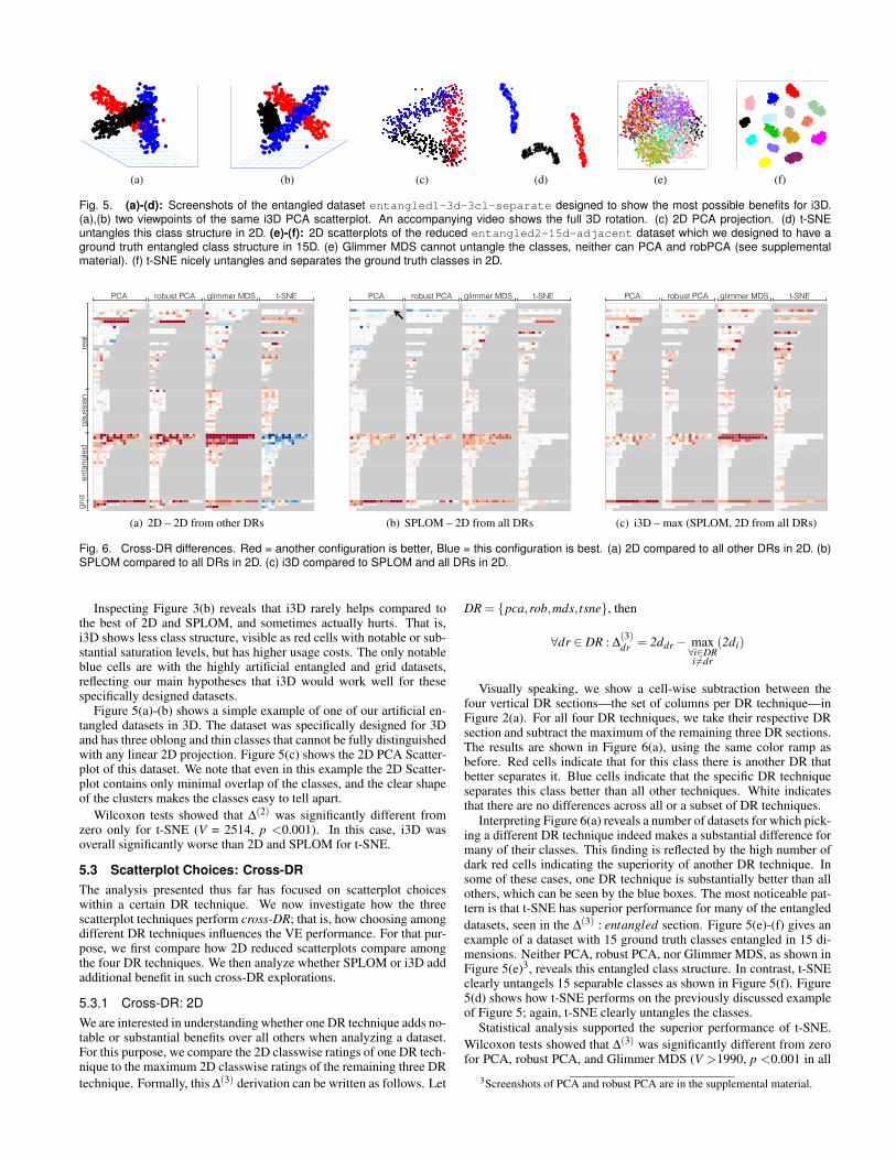
test

one

two

three

●●

●

● ●●

●

●

●

●

● ●

●

●

●

●

●

●

●●

●

●

●●

●

●

●

●

●

●

●

●

●

●

●

●

●

●

●

●

●

●

●

●

●●

●

●

●

●

●

●

●

●

●

●

●

●

●

●

●

●

●

●

●

●●●

●

●

●

●●

●

●

●

●

●

●

●

●

●

●

●

●

●

●

● ●●

●

●●

● ●

●●

●

●

●

●

●

●

●

●

●

●●

●

●●

●

●

●

●

●

●●

●

●

●

●

●

●

●

●

●

●

●

●

●

●

●●● ●

●

●

●

●

●

●

●

●

●

●

●

●

●

●●

●

●

●

●●

●

●

●●

●

●

●

●●

●

●●

●

●

●

●

● ●

●

●

●

●

●●

●

●

●

●

●

●

●

● ●

●●

●

●

●

●

●●

●

●

●

●

●

●●

●

●

●

●

●

●

●

●

● ●

● ●

●

●

●

●●

●

●

●

●

●

●●

●

●

●

●

●

●

●

●

●

●

●

●●

●

●● ●

●

●

●

●

●

●

●

●

●

●

●

●

●

●●

● ●

●

●

●

●

●

●●

●

●

●●●

●

●

●●

●

●

●

●

●

●

●

●

●

●

●

●

●

●

●●

●●

●

●

●

●

●

●●

●

●●

●●

●

●● ●

●●

● ●

●

●

●

●

●

●

●

●

●

●

●

●●

●●

●

●●●

●

●●

●●

●●

●●

●

●

●

●

●

●●

●

●●●

●●●

●

●●

●●

●●

●●

●

●

●

●

●●●

●

●

●

●

●●

●

●

●●

●●

●

●●●●

●

●●

●

●

●●

●●

●●

●

●●

●●

●●

●

●●

●●●●

●

●

●

●●

●● ●

●

●●

●●●

●

●

●

●

●

●●

●●

●

●

●

●

●

●

● ●

●

●●

●

●

●

●

●

●

●

●

●

● ●

●

● ●●

●●

●

●

●

●

●

●

●

●

●

●

●

●

●

●

●

●

●●●

●

●

●

●

●●

●

●

● ●

●

● ●

●

●

●

●

●

●

●●

●

●

●

●●

●

●

●

●●

●●

●

●●

●●

●

●

●

●

●

●

●

● ●

●

●●

●

●

●

●

●

●

●

●

●

●

●

●

●

●●●

●

●●

●

●

●

●

●

●

●●

●●

●●

●●

●

●

●

●

●

●

●

●

●●

●

●

●

●●●

●

●●

●●

●

●●

● ●●

●

●

●

●

(a)

test

one

two

three

●●

●

● ●●

●

●

●

●

● ●

●

●

●

●

●

●

●●

●

●

●●

●

●

●

●

●

●

●

●

●

●

●

●

●

●

●

●

●

●

●

●

●●

●

●

●

●

●

●

●

●

●

●

●

●

●

●

●

●

●

●

●

●●●

●

●

●

●●

●

●

●

●

●

●

●

●

●

●

●

●

●

●

● ●●

●

●●

● ●

●●

●

●

●

●

●

●

●

●

●

●●

●

●●

●

●

●

●

●

●●

●

●

●

●

●

●

●

●

●

●

●

●

●

●

●●● ●

●

●

●

●

●

●

●

●

●

●

●

●

●

●●

●

●

●

●●

●

●

●●

●

●

●

●●

●

●●

●

●

●

●

● ●

●

●

●

●

●●

●

●

●

●

●

●

●

● ●

●●

●

●

●

●

●●

●

●

●

●

●

●●

●

●

●

●

●

●

●

●

● ●

● ●

●

●

●

●●

●

●

●

●

●

●●

●

●

●

●

●

●

●

●

●

●

●

●●

●

●● ●

●

●

●

●

●

●

●

●

●

●

●

●

●

●●

● ●

●

●

●

●

●

●●

●

●

●●●

●

●

●●

●

●

●

●

●

●

●

●

●

●

●

●

●

●

●●

●●

●

●

●

●

●

●●

●

●●

●●

●

●● ●

●●

● ●

●

●

●

●

●

●

●

●

●

●

●

●●

●●

●

●●●

●

●●

●●

●●

●●

●

●

●

●

●

●●

●

●●●

●●●

●

●●

●●

●●

●●

●

●

●

●

●●●

●

●

●

●

●●

●

●

●●

●●

●

●●●●

●

●●

●

●

●●

●●

●●

●

●●

●●

●●

●

●●

●●●●

●

●

●

●●

●● ●

●

●●●●

●

●

●

●

●

●

●●

●●

●

●

●

●

●

●

● ●

●

●●

●

●

●

●

●

●

●

●

●

● ●

●

● ●●

●●

●

●

●

●

●

●

●

●

●

●

●

●

●

●

●

●

●●●

●

●

●

●

●●

●

●

● ●

●

● ●

●

●

●

●

●

●

●●

●

●

●

●●

●

●

●

●●

●●

●

●●

●●

●

●

●

●

●

●

●

● ●

●

●●

●

●

●

●

●

●

●

●

●

●

●

●

●

●●●

●

●●

●

●

●

●

●

●

●●

●●

●●

●●

●

●

●

●

●

●

●

●

●●

●

●

●

●●●

●

●●

●●

●

●●

● ●●

●

●

●

●

(b) (c)−30 −20 −10 0 10 20 30

−20

−10

010

2030

.x

.y

(d)−6 −4 −2 0 2 4 6

−4−2

02

46

.x

.y

(e)−30 −20 −10 0 10 20 30

−30

−20

−10

010

2030

.x

.y

(f)

Fig. 5. (a)-(d): Screenshots of the entangled dataset entangled1-3d-3cl-separate designed to show the most possible benefits for i3D.(a),(b) two viewpoints of the same i3D PCA scatterplot. An accompanying video shows the full 3D rotation. (c) 2D PCA projection. (d) t-SNEuntangles this class structure in 2D. (e)-(f): 2D scatterplots of the reduced entangled2-15d-adjacent dataset which we designed to have aground truth entangled class structure in 15D. (e) Glimmer MDS cannot untangle the classes, neither can PCA and robPCA (see supplementalmaterial). (f) t-SNE nicely untangles and separates the ground truth classes in 2D.

real

gaus

sian

enta

ngle

dgr

id

PCA robust PCA glimmer MDS t-SNEPCAPCAPCAPCAPCAPCAPCAPCAPCAPCAPCAPCAPCAPCAPCAPCA robPCArobPCArobPCArobPCArobPCArobPCArobPCArobPCArobPCArobPCArobPCArobPCArobPCArobPCArobPCArobPCA GLIMMERGLIMMERGLIMMERGLIMMERGLIMMERGLIMMERGLIMMERGLIMMERGLIMMERGLIMMERGLIMMERGLIMMERGLIMMERGLIMMERGLIMMERGLIMMER t-SNEt-SNEt-SNEt-SNEt-SNEt-SNEt-SNEt-SNEt-SNEt-SNEt-SNEt-SNEt-SNEt-SNEt-SNEt-SNE

abalone 0.0 0.0 0.0 0.0 0.0 0.0 0.0 0.0 0.0 0.0 0.0 0.0 0.0 0.0 0.0 0.0 0.0 0.0 0.0 0.0 0.0 0.0 0.0 0.0 0.0 0.0 0.0 0.0 0.0 0.0 0.0 0.0 0.0 0.0 0.0 0.0 0.0 0.0 0.0 0.0 0.0 0.0 0.0 0.0 0.0 0.0 0.0 0.0

cars03Cropped_d2 0.0 0.0 0.0 0.0 0.0 0.0 0.0 0.0 0.0 0.0 0.0 0.0 0.0 0.0 0.0 0.0 0.0 0.0 0.0 0.0 0.0 0.0 0.0 0.0 0.0 0.0 0.0 0.0 0.0 0.0 0.0 0.0 0.0 0.0 0.0 0.0 0.0 0.0 0.0 0.0 0.0 0.0 0.0 0.0 0.0 0.0 0.0 0.0

italianwines -1.0 0.0 0.0 -0.5 0.0 -1.0 -0.5 -1.0 -1.0 0.0 -1.0 -3.0 -2.5 -1.0 0.0 0.0 -0.5 0.0 -1.0 -0.5 -1.0 -1.0 0.0 -1.0 -3.0 -2.5 -0.5 0.0 0.0 0.5 0.0 -1.0 0.0 1.0 1.0 0.0 0.0 2.0 1.5 0.5 0.0 0.0 -0.5 0.0 1.0 0.0 -1.0 -1.0 0.0 0.0 -2.0 -1.5

worldmap 0.0 0.0 -2.0 -1.0 0.0 0.0 0.0 -2.0 0.0 -2.5 -1.0 0.0 0.0 0.0 0.0 0.0 -2.0 0.0 -3.0 -1.0 -3.0 -1.5 -0.5 0.0 0.0 -2.0 -4.0 -0.5 0.0 0.0 0.0 0.0 0.0 -3.0 0.0 0.0 0.0 0.0 0.0 0.0 0.0 0.0 0.0 0.0 0.0 0.0 2.0 0.0 0.0 0.0 0.0 -1.0

cars03Cropped_d3 0.0 1.0 0.0 0.0 0.0 0.0 0.5 0.0 2.0 0.5 0.0 1.5 0.0 -1.0 0.0 0.0 0.0 0.0 -0.5 0.0 -2.0 -2.0 0.0 -1.5 0.0 -1.0 0.0 -1.0 0.0 0.0 -0.5 0.0 -2.0 -0.5 0.0 -1.5

fisheries_clusteredByEscapementTarget -3.5 -3.5 -3.5 -3.5 -3.5 -3.5 -3.5 -3.5 -3.5 -3.5 -3.5 2.0 1.0 1.0 1.0 0.5 0.0 0.0 0.0 0.0 0.0 0.0 -2.0 -1.0 -1.0 -1.0 -0.5 0.0 0.0 0.0 0.0 0.0 0.0 -3.0 -2.0 -2.0 -2.0 -2.0 -3.0 -2.0 -2.0 -3.0 -3.0 -2.5

fisheries_clusteredByHarvestRule 0.0 -0.5 -2.0 -4.0 -4.0 -4.0 -4.0 -4.0 -4.0 -4.0 -4.0 0.0 -0.5 -2.0 -4.0 -4.0 -4.0 -4.0 -4.0 -4.0 -4.0 -4.0 0.0 0.0 0.0 1.0 1.5 1.5 1.5 1.5 1.5 2.0 2.0 0.0 0.0 0.0 -1.0 -1.5 -1.5 -1.5 -1.5 -1.5 -2.0 -2.0

yeast 1.0 1.0 1.0 1.0 1.0 2.0 1.5 1.0 1.0 1.0

ecoliproteins 0.0 1.0 0.0 0.0 0.0 -0.5 -4.0 0.5 0.0 -1.0 0.0 0.0 0.0 0.5 4.0 -0.5

efashion 0.0 0.0 0.0 0.0 0.0 0.0 0.0 0.0 0.0 0.0 0.0 0.0 0.0 0.0 0.0 0.0 0.0 0.0 0.0 0.0 0.0 0.0 0.0 -0.5

tse300 -0.5 0.0 0.5 0.0 -0.5 0.0 0.0 0.0 -0.5 0.0 -0.5 0.0 -0.5 0.0 0.0 0.0 0.5 -1.5 -0.5 -2.0 0.5 -1.0 -2.5 0.0 -4.0 -3.0 -2.0 -3.5 -4.0 -1.5 -3.0 0.0

cereal 1.0 0.0 0.0 0.0 0.0 0.0 0.0 0.0 0.0 0.0 0.0 0.0 0.0 0.0 0.0 0.0 0.0 0.0 0.0 0.0 0.0

shuttle_big 0.0 0.0 0.0 -0.5 -0.5 0.5 0.5 0.0 0.0 0.0 0.5 0.5 -0.5 -0.5

shuttle_small 0.5 0.0 0.0 -1.0 0.0 3.0 3.5 -0.5 0.0 0.0 1.0 0.0 -3.0 -3.5

musicnetgroups 0.0 0.0 0.0 -1.0 0.0 0.0 0.0 0.0 0.0 1.0 0.0 0.0 0.0 0.0 0.0 -1.5 -1.0 0.0 0.0 0.0 0.0 -4.0 -4.0 -2.5

hiv 1.0 0.0 -1.0 -0.5 0.0 0.0 -1.0 0.0 1.0 0.5 0.0 0.0

bbdm13 2.5 2.0 0.0 1.0 2.0 -3.0 -2.0 0.0 -1.0 -2.0 -2.5 -2.0 0.0 -1.0 -2.0

white_ballance 0.0 -1.0 0.0 0.5 0.0 0.0 -1.0 0.0 -0.5 0.0 0.0 1.0 -0.5 -0.5 -0.5

world_11d -0.5 -1.5 -2.0 0.0 -0.5 -0.5 -0.5 -2.5 -0.5 -2.0 0.5 0.5 2.0 0.0 0.5 -2.5 -1.5 -2.5 -1.0 -2.0

world_9d -1.0 -1.5 -3.5 0.5 -1.0 1.0 1.5 3.5 -0.5 1.0 -3.0 -2.5 -3.5 -2.0 -3.0

boston -1.5 -1.5 -3.0 -1.0 -1.0 -3.0 -0.5 0.5 0.0 0.5 -0.5 0.0

iris 0.0 0.5 0.5 0.0 -0.5 -0.5 0.0 -1.0 -1.0 0.0 -2.5 -2.5

olive -2.0 0.0 -1.5 -2.0 0.0 -1.5 -0.5 0.0 -0.5 0.5 0.0 0.5

swanson 0.0 0.0 -0.5 0.0 0.0 -1.5 0.0 0.0 0.5

wine -1.0 -1.5 -2.5 0.0 -1.5 -2.5 -0.5 0.5 1.0 0.0 -0.5 -1.0

breast-cancer-wisconsin 0.0 0.0 0.0 0.0 -0.5 -1.0

cars03Cropped_d1 -1.5 -1.5 1.5 1.5 -1.5 -1.5

ionosphere -0.5 -0.5 0.5 0.5

parkinsons_abs_croped -1.5 -1.5 -1.5 -1.5 1.5 1.5

spambase 0.0 0.5 0.0 -0.5

wdbc_class_1_2 -0.5 -0.5 0.0 0.0 0.0 0.0 -2.5 -2.0

n100-d10-c5-spr0.1-out0 0.5 0.0 1.0 0.0 0.5 -3.0 0.0 -4.0 0.0 -3.0 -2.0 -2.0 -3.0 -2.5 -2.5 -0.5 -0.5 -1.0 -1.5 -0.5

n100-d10-c5-spr0.2-out0 0.0 -1.0 0.0 0.0 0.0 0.0 1.0 0.0 0.0 0.0 -1.0 -2.0 -0.5 -1.5 -0.5 -1.0 -2.5 -0.5 -2.5 -0.5

n100-d5-c5-spr0.1-out0 0.0 0.0 0.0 0.0 -0.5 0.0 0.0 0.0 0.0 -0.5 -0.5 -2.0 -0.5 -1.0 0.5 -0.5 -2.0 -1.0 -2.0 -1.5

n100-d5-c5-spr0.2-out0 0.0 -0.5 0.0 0.5 -0.5 -0.5 -1.0 -0.5 -1.0 -0.5 0.0 0.5 0.0 -0.5 0.5 -1.0 -1.0 -0.5 -1.0 -0.5

n500-d10-c5-spr0.1-out0 0.0 -1.5 -1.5 -0.5 0.0 0.0 -1.5 -1.5 -0.5 0.0 -1.0 -3.0 -2.0 -0.5 0.0 0.0 1.5 1.5 0.5 0.0

n500-d10-c5-spr0.2-out0 0.0 0.0 -0.5 -1.5 0.0 0.0 0.0 -0.5 -1.5 0.0 -1.0 -1.5 -0.5 -1.5 -1.5 -1.0 -1.0 0.5 1.5 -1.0

n500-d5-c5-spr0.1-out0 -0.5 0.0 -0.5 0.0 0.0 -0.5 0.0 -0.5 0.0 0.0 -0.5 -1.0 0.0 0.0 0.0 0.5 -1.0 0.0 -0.5 0.0

n500-d5-c5-spr0.2-out0 -1.0 0.0 -0.5 -0.5 -0.5 1.0 0.0 0.5 0.5 0.5 -1.0 -0.5 -0.5 -0.5 -2.0 -1.0 -0.5 -0.5 -0.5 -2.0

n100-d10-c3-spr0.1-out0 0.0 0.0 0.0 0.0 0.0 0.0 0.0 -0.5 0.0 -1.5 -2.0 -1.0

n100-d10-c3-spr0.2-out0 0.0 0.0 0.0 0.0 0.0 0.0 -0.5 -1.0 -1.0 -2.5 -1.5 -1.5

n100-d5-c3-spr0.1-out0 0.0 0.0 0.0 0.0 -0.5 0.0 0.0 0.0 0.0 0.0 -1.0 -0.5

n100-d5-c3-spr0.2-out0 0.0 0.5 0.0 -0.5 -0.5 0.0 -2.0 -2.5 -2.5 0.0 -1.0 -1.0

n500-d10-c3-spr0.1-out0 0.0 0.0 0.0 0.0 0.0 0.0 0.0 0.0 0.0 0.0 0.0 0.0

n500-d10-c3-spr0.2-out0 0.0 0.0 0.0 0.0 0.0 0.0 -1.0 -1.0 -1.0 -2.0 -1.5 -1.0

n500-d5-c3-spr0.1-out0 0.0 0.0 0.0 0.0 0.0 0.0 0.0 -0.5 -0.5 0.0 -0.5 -0.5

n500-d5-c3-spr0.2-out0 0.5 0.0 -0.5 -0.5 0.0 0.5 -1.5 -0.5 -1.0 -1.5 -0.5 -1.0

interleaved_100_200_15d_0_notcramped_notrotated -2.0 -2.5 -4.0 -4.0 -3.0 -1.5 -4.0 -2.5 -4.0 -2.0 -3.5 -4.0 -2.0 -3.5 -1.5 -2.5 -2.5 -4.0 -4.0 -3.5 -1.0 -4.0 -2.5 -4.0 -1.5 -3.5 -4.0 -1.5 -3.5 -1.0 -4.0 -4.0 -4.0 -4.0 -4.0 -4.0 -4.0 -4.0 -4.0 -4.0 -4.0 -4.0 -4.0 -4.0 -4.0 2.0 2.5 4.0 4.0 3.0 1.0 4.0 2.5 4.0 1.5 3.5 4.0 1.5 3.5 1.0

interleaved_100_200_15d_25_cramped_rotated -4.0 -2.0 -4.0 -1.5 -4.0 -3.0 -4.0 -4.0 -4.0 -2.0 -3.0 -3.0 -3.0 -2.0 -1.5 -4.0 -2.0 -4.0 -1.5 -4.0 -3.0 -4.0 -4.0 -4.0 -2.0 -3.0 -3.0 -3.0 -2.0 -1.5 -4.0 -4.0 -4.0 -4.0 -4.0 -3.0 -4.0 -4.0 -4.0 -4.0 -4.0 -4.0 -4.0 -3.0 -4.0 4.0 2.0 4.0 1.5 4.0 3.0 4.0 4.0 4.0 2.0 3.0 3.0 3.0 2.0 1.5

interleaved_100_200_10d_0_notcramped_notrotated -0.5 0.0 -1.5 0.0 -4.0 -4.0 -2.0 -0.5 -3.5 -3.5 -1.0 0.0 -1.5 0.0 -4.0 -4.0 -2.0 -0.5 -3.5 -4.0 -3.0 -2.0 -3.0 -2.0 -3.5 -3.5 -3.5 -2.0 -3.5 -3.5 0.5 0.0 1.5 0.0 3.5 3.5 2.0 0.5 3.5 3.5

interleaved_100_200_10d_25_cramped_rotated -2.5 -2.0 -3.0 -4.0 -2.5 -1.0 -2.5 -1.0 -1.0 -4.0 -2.5 -2.5 -3.0 -4.0 -3.0 -1.0 -2.5 -1.0 -1.0 -4.0 -4.0 -4.0 -3.5 -4.0 -4.0 -4.0 -3.5 -4.0 -4.0 -4.0 2.5 2.0 3.0 4.0 2.5 1.0 2.5 1.0 1.0 4.0

interleaved_100_200_6d_0_notcramped_notrotated -2.5 -2.0 -2.0 -0.5 -1.5 0.0 -2.5 -1.0 -2.0 -1.0 -1.0 0.0 -3.5 -1.0 -1.5 -2.0 -1.5 0.0 2.5 1.0 1.5 0.5 1.0 0.0

interleaved_100_200_6d_25_cramped_rotated 0.0 -1.5 -1.0 -0.5 -0.5 -1.5 0.0 -1.5 -1.0 -0.5 -0.5 -1.5 -0.5 -1.5 -1.0 -1.5 -1.0 -1.5 0.0 1.5 1.0 0.5 0.5 1.5

interleaved_100_200_5d_0_notcramped_notrotated -2.0 -1.5 -1.5 -1.0 -1.0 -2.0 -1.0 -1.5 -1.0 -1.0 0.0 -3.0 -1.0 -1.5 -1.5 0.0 1.0 1.0 1.0 1.0

interleaved_100_200_5d_25_cramped_rotated 0.0 -1.5 -0.5 -0.5 -0.5 -0.5 -1.5 0.0 -0.5 -0.5 -1.0 -2.0 -0.5 -1.0 -3.0 0.0 1.5 0.0 0.5 0.5

JavierGeneratedData_3dinterleaved_5classes -0.5 -1.0 0.0 -1.0 0.0 0.0 -0.5 -1.0 -0.5 -1.0 -0.5 -1.0 0.0 -1.0 0.0 0.0 0.5 0.0 0.5 0.0

interleaved_100_200_4d_0_notcramped_notrotated -0.5 -1.0 -0.5 0.0 -0.5 -1.0 -0.5 0.0 -1.0 -2.0 -1.0 -1.0 0.5 1.0 0.5 0.0

interleaved_100_200_4d_25_cramped_rotated -2.5 -1.0 -2.0 -0.5 -2.5 -1.0 -2.0 -0.5 0.0 0.0 -2.0 -1.0 0.0 0.0 2.0 0.5

JavierGeneratedData_3dinterleaved_4classes -0.5 -0.5 0.0 -0.5 -0.5 -1.0 -0.5 -1.0 0.0 0.0 0.0 0.0 0.0 0.0 0.0 0.0

interleaved_100_500_3_25_cramped_rotated 0.0 0.0 0.0 0.0 0.0 0.0 0.0 0.0 0.0 0.0 0.0 -0.5

interleaved_250_500_3_0_notCramped_rotated 0.0 0.0 0.0 0.0 0.0 0.0 0.0 0.0 0.0 -0.5 -0.5 -1.0

JavierGeneratedData_3dinterleaved_3classes -0.5 -0.5 -0.5 -0.5 -0.5 -0.5 0.0 0.0 0.0 0.0 0.0 0.0

ms_interleaved_120_240_3d_25_centeredClusters 0.0 0.0 0.0 0.0 0.0 0.0 -0.5 -0.5 -0.5 -1.0 -2.0 -1.5

ms_interleaved_120_240_3d_50_centeredClusters 0.0 0.0 0.0 0.0 0.0 0.0 0.0 0.0 0.0 -1.5 -1.5 -1.5

ms_interleaved_40_80_3d_0 0.0 0.0 0.0 0.0 0.0 0.0 0.0 0.0 0.0 -1.5 -1.5 -0.5

ms_interleaved_40_80_3d_50 0.0 0.0 0.0 0.0 0.0 0.0 0.0 0.0 0.0 -0.5 -0.5 -0.5

ms_interleaved_400_800_3d_0 0.0 0.0 0.0 0.0 0.0 0.0 0.0 0.0 0.0 -0.5 -0.5 -2.5

ms_interleaved_400_800_3d_50 -0.5 -0.5 -0.5 -0.5 -0.5 -0.5 0.5 0.5 0.5 -1.5 -1.5 -1.5


ms_interleaved_60_120_3d_25_centeredClusters 0.0 0.0 0.0 0.0 0.0 0.0 0.0 -0.5 -0.5 -0.5 -1.0 -0.5

ms_interleaved_60_120_3d_50_centeredClusters -0.5 -0.5 -0.5 -0.5 -0.5 -0.5 0.5 0.5 0.5 -2.0 -2.0 -2.0

grid6_4d -3.5 -2.5 -2.5 -3.5 -4.0 -4.0 -4.0 -4.0 -3.0 -4.0 -3.5 -3.0 -4.0 -4.0 -4.0 -4.0 -3.5 -2.5 -2.5 -3.5 1.5 2.0 0.0 -4.0 -3.0 -4.0 -3.5 -3.0 0.0 0.0 0.0 0.5 -3.0 -2.0 -2.0 -3.0 -3.5 -3.5 -3.5 -3.5 -2.5 -3.5 -3.0 -2.5 -3.5 -3.5 -3.5 -3.5 3.0 2.0 2.0 3.0 -1.5 -2.0 0.0 3.5 2.5 3.5 3.0 2.5 0.0 0.0 0.0 -0.5

grid10_3d -3.0 -4.0 -3.0 -4.0 1.0 0.0 1.0 0.5 0.0 -1.0 0.5 -3.5 -3.5 -1.0 -1.0 -1.0 -1.5 -2.5 -1.0 -2.5 -2.5 -2.0 -2.5 -2.5 0.0 1.0 -0.5 2.5 -1.0 0.0 -1.5 -0.5

twosquare-nome -3.5 -2.5 0.0 0.0 -3.5 -2.5 0.0 0.0 -3.5 -3.5 -4.0 -4.0 3.5 2.5 -0.5 -0.5

UnEvenDensity-nome 0.0 0.0 0.0 0.0 -0.5 0.0

(a) 2D – 2D from other DRs

PCA robust PCA glimmer MDS t-SNEdataset family pca -SPLOM better than 2dpca -SPLOM better than 2dpca -SPLOM better than 2dpca -SPLOM better than 2dpca -SPLOM better than 2dpca -SPLOM better than 2dpca -SPLOM better than 2dpca -SPLOM better than 2dpca -SPLOM better than 2dpca -SPLOM better than 2dpca -SPLOM better than 2dpca -SPLOM better than 2dpca -SPLOM better than 2dpca -SPLOM better than 2d robpca -SPLOM better than 2drobpca -SPLOM better than 2drobpca -SPLOM better than 2drobpca -SPLOM better than 2drobpca -SPLOM better than 2drobpca -SPLOM better than 2drobpca -SPLOM better than 2drobpca -SPLOM better than 2drobpca -SPLOM better than 2drobpca -SPLOM better than 2drobpca -SPLOM better than 2drobpca -SPLOM better than 2drobpca -SPLOM better than 2drobpca -SPLOM better than 2d glimmer - SPLOM better than 2dglimmer - SPLOM better than 2dglimmer - SPLOM better than 2dglimmer - SPLOM better than 2dglimmer - SPLOM better than 2dglimmer - SPLOM better than 2dglimmer - SPLOM better than 2dglimmer - SPLOM better than 2dglimmer - SPLOM better than 2dglimmer - SPLOM better than 2dglimmer - SPLOM better than 2dglimmer - SPLOM better than 2dglimmer - SPLOM better than 2dglimmer - SPLOM better than 2d tsne - SPLOM better than 2dtsne - SPLOM better than 2dtsne - SPLOM better than 2dtsne - SPLOM better than 2dtsne - SPLOM better than 2dtsne - SPLOM better than 2dtsne - SPLOM better than 2dtsne - SPLOM better than 2dtsne - SPLOM better than 2dtsne - SPLOM better than 2dtsne - SPLOM better than 2dtsne - SPLOM better than 2dtsne - SPLOM better than 2dtsne - SPLOM better than 2d

abalone real 0.0 0.0 0.0 0.0 0.0 0.0 0.0 0.0 0.0 0.0 0.0 0.0 0.0 0.0 0.0 0.0 0.0 0.0 0.0 0.0 0.0 0.0 0.0 0.0 0.0 0.0 0.0 0.0 0.0 0.0 0.0 0.0 0.0 0.0 0.0 0.0 0.0 0.0 0.0 0.0 0.0 0.0 0.0 0.0 0.0 0.0 0.0 0.0

cars03Cropped_d2 real 0.0 0.0 0.0 0.0 0.0 0.0 0.0 0.0 0.0 0.0 0.0 0.0 0.0 0.0 0.0 0.0 0.0 0.0 0.0 0.0 0.0 0.0 0.0 0.0 0.0 0.0 0.0 0.0 0.0 0.0 0.0 0.0 0.0 0.0 0.0 0.0 0.0 0.0 0.0 0.0 0.0 0.0 0.0 0.0 0.0 0.0 0.0 0.0

italianwines real 3.0 3.0 1.0 0.5 1.5 2.0 2.0 2.0 2.0 2.5 2.5 1.0 1.5 3.0 3.0 1.0 0.5 2.5 2.0 2.0 2.0 1.5 2.5 2.0 1.0 1.5 -1.0 0.5 1.5 0.0 0.5 -0.5 0.0 -0.5 -0.5 0.0 0.5 0.0 1.0 0.5 1.0 1.0 0.0 0.5 -1.0 0.5 -0.5 -1.0 0.0 0.5 -1.5 0.0

worldmap real 0.0 0.0 0.0 0.0 0.0 0.0 0.0 0.0 0.0 -0.5 0.0 0.0 0.0 0.0 0.0 0.0 0.0 0.0 0.0 0.0 0.0 0.0 0.0 0.0 0.0 -0.5 0.0 0.0 0.0 0.0 0.0 0.0 0.0 0.0 0.0 0.0 0.0 0.0 0.0 0.0 0.0 0.0 0.0 0.0 0.0 0.0 0.0 0.0 0.0 0.0 0.0 0.0

cars03Cropped_d3 real 0.0 0.0 0.0 0.0 0.0 0.5 1.5 0.5 0.5 0.5 0.0 -0.5 0.0 0.5 0.0 0.0 0.5 0.0 2.0 0.0 -1.5 0.5 0.0 -1.5 0.0 -1.0 0.0 -1.0 0.0 0.0 -0.5 0.0 -2.0 -1.0 0.0 -1.5

fisheries_clusteredByEscapementTarget real -1.0 -1.0 -1.0 -0.5 -0.5 -0.5 -0.5 -0.5 -0.5 -0.5 -0.5 0.0 0.0 0.0 0.0 0.0 0.0 0.0 0.0 0.0 0.0 0.0 0.0 0.0 0.5 0.0 0.0 0.0 0.0 0.5 0.5 0.5 0.5 -1.5 -1.0 -1.0 -1.0 -0.5 -1.0 -1.0 -1.0 -1.0 -1.5 -1.5

fisheries_clusteredByHarvestRule real 0.0 0.0 0.0 0.0 0.0 0.0 0.0 0.0 0.0 0.0 0.0 0.0 0.0 0.0 0.0 -0.5 0.0 0.0 0.0 0.0 0.0 0.0 0.0 0.0 0.0 0.0 0.0 0.0 0.0 0.0 0.0 0.0 0.0 0.0 0.0 0.0 0.0 -1.0 -3.5 -3.5 -3.5 -3.5 -3.0 -3.0

yeast real 0.0 0.0 0.0 0.0 0.0 -1.0 -0.5 0.0 0.0 0.0

ecoliproteins real 0.0 0.0 0.0 4.0 0.0 2.5 0.0 0.5 0.0 -0.5 0.0 1.0 -0.5 2.0 0.0 1.5

efashion real 0.0 0.0 0.0 0.0 0.0 0.0 0.0 0.0 0.0 0.0 0.0 0.0 0.0 0.0 0.0 0.0 0.0 0.0 0.0 0.0 -0.5 0.0 0.0 -1.0

tse300 real -0.5 0.0 -0.5 0.0 -0.5 0.5 0.0 0.0 -0.5 0.0 -0.5 0.0 -0.5 1.0 0.0 0.0 -0.5 -1.5 -0.5 -2.0 -0.5 1.0 -2.0 0.0 -4.0 -3.0 -2.0 -3.5 -4.0 -1.5 -3.0 0.0

cereal real 0.0 0.0 0.0 0.0 0.0 0.0 0.0 0.0 0.0 0.0 0.0 0.0 0.0 0.0 0.0 0.0 0.0 0.0 0.0 0.0 0.0

shuttle_big real 0.0 0.0 0.0 -0.5 -0.5 0.0 0.0 0.0 0.0 0.0 -0.5 -0.5 -0.5 -0.5

shuttle_small real 0.5 0.0 0.5 0.0 0.5 0.0 0.0 -0.5 0.0 0.0 -1.0 -0.5 -4.0 -4.0

musicnetgroups real 0.0 0.0 0.0 -0.5 0.0 0.0 0.0 0.0 0.0 0.0 0.0 0.0 0.0 0.0 0.0 -1.5 -0.5 0.0 0.0 0.0 0.0 -1.0 -3.0 -0.5

hiv real 1.0 1.0 -1.0 0.5 0.5 0.0 0.0 1.0 0.0 0.0 0.0 0.0

bbdm13 real 1.0 1.0 2.5 1.5 2.0 -3.0 -2.0 0.0 -1.0 -2.0 -2.5 -2.0 0.0 -1.0 -2.0

white_ballance real 2.0 0.5 0.0 0.0 0.5 0.5 1.0 0.5 1.5 0.5 0.0 0.5 0.0 0.5 -0.5

world_11d real 0.0 0.0 0.5 0.5 0.0 -0.5 0.0 0.5 0.0 0.0 0.0 0.5 1.5 1.5 0.5 -1.0 -1.0 -0.5 -0.5 -0.5

world_9d real 0.0 0.0 -0.5 0.0 0.5 0.0 0.5 -0.5 -1.0 0.5 -1.0 -0.5 -2.5 -1.5 0.0

boston real -0.5 1.0 0.5 -1.0 -1.0 -3.0 -0.5 1.0 0.5 -0.5 0.5 0.5

iris real 0.0 0.0 0.0 0.0 -0.5 -0.5 0.0 -0.5 -0.5 0.0 -1.5 -2.0

olive real -2.0 0.0 -1.5 -2.0 0.0 -1.5 -0.5 0.0 -0.5 0.0 0.0 0.0

swanson real 0.0 0.0 -0.5 0.0 0.0 -1.5 0.0 0.0 0.0

wine real -0.5 0.0 -1.0 0.0 0.5 -0.5 -0.5 0.0 0.5 0.5 0.5 0.5

breast-cancer-wisconsin real 0.0 0.0 0.0 0.0 0.5 0.5

cars03Cropped_d1 real -0.5 -0.5 0.0 0.0 -1.0 -1.0

ionosphere real 0.5 1.0 0.0 0.0

parkinsons_abs_croped real -1.5 -2.0 -1.0 -1.5 0.0 -0.5

spambase real 2.0 1.5 0.5 0.0

wdbc_class_1_2 real 0.5 0.5 0.0 0.0 0.0 0.0 -1.5 -1.0

n100-d10-c5-spr0.1-out0 gaussian 1.0 0.0 0.0 0.0 0.5 1.0 0.0 -0.5 0.0 0.5 0.5 -1.0 0.0 -1.5 -0.5 0.5 -0.5 -0.5 -1.5 0.0

n100-d10-c5-spr0.2-out0 gaussian 0.5 -1.0 1.5 0.0 1.5 -0.5 -0.5 1.5 0.0 2.0 -0.5 -1.5 1.0 -1.0 1.0 -0.5 -1.5 1.5 -0.5 1.0

n100-d5-c5-spr0.1-out0 gaussian 0.0 0.0 0.0 0.0 -0.5 0.0 0.0 0.0 0.0 -0.5 -0.5 -1.5 -0.5 -1.5 0.0 0.0 -0.5 -0.5 -1.0 -1.0

n100-d5-c5-spr0.2-out0 gaussian 0.0 -0.5 0.0 0.0 -0.5 -0.5 -0.5 0.5 -0.5 -0.5 0.0 0.0 0.0 -0.5 -1.0 -1.0 -0.5 -0.5 0.0 0.0

n500-d10-c5-spr0.1-out0 gaussian 0.0 0.0 0.0 0.5 0.0 0.0 0.0 0.0 0.0 0.0 -0.5 -2.5 -1.5 -0.5 0.0 0.0 -0.5 -1.0 0.0 0.0

n500-d10-c5-spr0.2-out0 gaussian 0.0 0.5 0.5 0.5 0.0 0.5 0.0 0.5 1.0 0.0 -1.0 -0.5 0.0 -0.5 -1.0 0.0 -0.5 0.0 0.0 -1.5

n500-d5-c5-spr0.1-out0 gaussian -0.5 0.0 0.0 0.0 0.5 -0.5 0.0 0.0 0.0 0.5 -0.5 -0.5 0.0 1.0 0.0 0.0 -0.5 0.0 0.0 1.0

n500-d5-c5-spr0.2-out0 gaussian -1.0 0.0 0.5 -0.5 -0.5 -0.5 0.0 0.5 0.0 0.5 -1.0 0.0 0.0 0.5 -0.5 -0.5 0.5 0.5 0.0 -0.5

n100-d10-c3-spr0.1-out0 gaussian 0.0 0.0 0.0 0.0 0.0 0.0 0.0 0.0 0.0 0.0 -1.0 -1.0

n100-d10-c3-spr0.2-out0 gaussian 0.0 0.0 0.0 0.5 0.0 0.0 0.0 -0.5 0.5 -0.5 -0.5 -0.5

n100-d5-c3-spr0.1-out0 gaussian 0.0 0.0 0.0 0.0 0.0 0.0 0.0 0.0 0.0 0.0 0.0 0.0

n100-d5-c3-spr0.2-out0 gaussian 0.5 0.0 0.0 0.5 -0.5 0.0 -0.5 -1.0 -1.0 0.5 -0.5 0.0


n500-d10-c3-spr0.2-out0 gaussian 0.0 0.0 0.0 0.0 0.0 0.0 -0.5 -0.5 -0.5 -2.0 -1.0 -1.5

n500-d5-c3-spr0.1-out0 gaussian 0.0 0.0 0.0 0.0 0.0 0.0 0.0 -0.5 -0.5 0.0 -0.5 -0.5

n500-d5-c3-spr0.2-out0 gaussian 0.0 0.0 -0.5 -0.5 0.0 0.0 -1.5 -0.5 -1.0 -1.5 -0.5 -1.0

interleaved_100_200_15d_0_notcramped_notrotated interleaved -1.0 -1.5 -2.5 -2.0 -2.5 -1.5 -2.0 -1.0 -2.5 -1.5 -0.5 -1.0 -2.5 -2.5 -1.5 -1.5 -2.0 -3.0 -1.5 -3.5 -1.0 -1.5 -1.0 -2.5 -1.0 -0.5 -1.5 -2.0 -2.5 -1.0 -3.0 -2.5 -3.0 -3.5 -2.5 -2.5 -2.0 -1.5 -2.5 -3.0 -2.5 -3.5 -2.5 -3.0 -2.0 0.0 0.0 0.0 0.0 0.0 0.0 0.0 0.0 0.0 0.0 0.0 0.0 0.0 0.0 0.0

interleaved_100_200_15d_25_cramped_rotated interleaved -4.0 -1.5 -3.0 -1.5 -0.5 -1.5 -2.5 -2.0 -3.0 -1.0 -2.5 -2.0 -3.5 -2.5 -1.5 -4.0 -1.5 -3.0 -1.5 -0.5 -1.0 -2.5 -2.5 -3.0 -1.5 -2.5 -2.5 -3.5 -2.5 -1.5 -3.0 -2.5 -3.5 -2.5 -1.5 -2.0 -1.5 -1.5 -3.0 -2.5 -3.0 -3.5 -3.0 -3.0 -3.0 0.0 0.0 0.0 0.0 0.0 0.5 0.0 0.0 0.0 0.0 0.0 0.0 0.0 0.0 0.0

interleaved_100_200_10d_0_notcramped_notrotated interleaved -0.5 0.0 -1.5 0.0 0.0 0.0 -2.0 -0.5 -1.5 -2.0 -0.5 -0.5 -1.5 0.0 0.0 -0.5 -2.0 -0.5 -2.5 -2.5 -2.0 -2.0 -2.0 -2.0 -1.0 -2.0 -2.0 -1.5 -2.5 -1.5 0.0 -0.5 -0.5 0.0 0.0 0.0 -1.0 0.0 0.0 0.0

interleaved_100_200_10d_25_cramped_rotated interleaved -1.5 -2.0 0.0 -1.5 -0.5 -1.5 -2.0 -1.5 -0.5 -2.0 -1.5 -2.0 0.0 -2.0 -0.5 -2.0 -2.0 -1.5 -1.0 -2.0 -2.0 -3.5 -2.0 -2.5 -1.5 -2.5 -1.5 -2.5 -2.0 -3.0 0.0 -1.0 0.0 0.0 0.0 0.0 0.0 0.0 0.0 0.0

interleaved_100_200_6d_0_notcramped_notrotated interleaved -1.5 -0.5 -0.5 -0.5 -0.5 0.0 -1.5 -0.5 -1.0 -1.0 -1.0 0.0 -2.0 -0.5 -1.0 -1.0 -0.5 -0.5 0.0 0.0 0.0 0.5 0.5 0.0

interleaved_100_200_6d_25_cramped_rotated interleaved 0.0 -1.0 -1.0 -0.5 -0.5 -0.5 0.0 -1.0 -1.0 -0.5 -0.5 -0.5 -1.0 -1.0 -1.0 -2.0 -1.0 -0.5 0.5 0.0 0.5 0.0 0.0 0.5

interleaved_100_200_5d_0_notcramped_notrotated interleaved -2.0 -1.5 -0.5 -0.5 -0.5 -1.5 -1.0 -1.0 -0.5 -0.5 0.0 -1.0 -0.5 0.0 -1.0 0.0 0.0 0.0 0.0 0.0

interleaved_100_200_5d_25_cramped_rotated interleaved 0.0 0.0 0.0 -1.0 -1.0 -0.5 0.0 0.0 -0.5 -0.5 -0.5 0.0 -0.5 -0.5 -1.0 0.0 0.0 0.5 0.0 0.0

JavierGeneratedData_3dinterleaved_5classes interleaved 0.0 -0.5 0.0 0.0 0.0 0.0 -0.5 0.0 0.0 0.0 0.0 0.0 0.0 -0.5 -0.5 0.5 0.0 0.0 0.0 0.0

interleaved_100_200_4d_0_notcramped_notrotated interleaved -0.5 -0.5 -0.5 0.5 -0.5 -0.5 -0.5 0.5 -1.5 -1.0 -1.0 0.5 0.0 0.0 0.0 1.0

interleaved_100_200_4d_25_cramped_rotated interleaved 0.0 -0.5 -1.0 -0.5 0.0 -0.5 -1.0 -0.5 0.5 0.0 -1.0 -0.5 0.5 0.0 0.5 0.0

JavierGeneratedData_3dinterleaved_4classes interleaved -0.5 -0.5 0.0 -0.5 -0.5 -0.5 -0.5 -1.0 0.0 0.0 -1.0 0.0 0.0 0.0 0.0 0.0

interleaved_100_500_3_25_cramped_rotated interleaved 0.0 0.0 0.0 0.0 0.0 0.0 0.0 0.0 -0.5 0.0 0.0 0.0

interleaved_250_500_3_0_notCramped_rotated interleaved 0.0 0.0 0.0 0.0 0.0 0.0 -0.5 -0.5 -0.5 -0.5 -1.0 -0.5

JavierGeneratedData_3dinterleaved_3classes interleaved -0.5 -0.5 -0.5 -0.5 -0.5 -0.5 0.0 -0.5 -0.5 0.0 0.0 0.0

ms_interleaved_120_240_3d_25_centeredClusters interleaved -0.5 -0.5 -0.5 -0.5 -0.5 -0.5 -1.0 -0.5 -0.5 -0.5 -0.5 -1.0

ms_interleaved_120_240_3d_50_centeredClusters interleaved 0.0 0.0 0.0 0.0 0.0 0.0 0.0 0.0 0.0 -1.5 -1.5 -1.5

ms_interleaved_40_80_3d_0 interleaved 0.0 0.0 0.0 0.0 0.0 0.0 -0.5 -0.5 -0.5 0.0 0.0 0.0

ms_interleaved_40_80_3d_50 interleaved 0.0 0.0 0.0 0.0 0.0 0.0 -0.5 -0.5 -0.5 -0.5 -0.5 -0.5

ms_interleaved_400_800_3d_0 interleaved 0.0 0.0 0.0 0.0 0.0 0.0 -0.5 -0.5 -0.5 -0.5 -0.5 -1.5

ms_interleaved_400_800_3d_50 interleaved -0.5 -0.5 -0.5 -0.5 -0.5 -0.5 -0.5 0.0 0.0 -1.5 -1.5 -1.5

ms_interleaved_60_120_3d_0_centeredClusters interleaved 0.0 0.0 0.0 0.0 0.0 0.0 0.0 0.0 0.0 0.0 0.0 0.0

ms_interleaved_60_120_3d_25_centeredClusters interleaved 0.0 0.0 0.0 0.0 0.0 0.0 0.0 -0.5 -0.5 0.0 -0.5 0.0

ms_interleaved_60_120_3d_50_centeredClusters interleaved -0.5 -0.5 -0.5 -0.5 -0.5 -0.5 0.0 0.0 0.0 -1.0 -1.0 -1.0

grid6_4d grid -3.5 -2.5 -2.5 -3.5 -4.0 -4.0 -4.0 -4.0 -3.0 -4.0 -3.5 -3.0 -4.0 -4.0 -4.0 -4.0 -3.0 -2.5 -2.5 0.5 0.0 0.0 0.0 0.0 1.0 0.0 -3.5 -3.0 0.0 -4.0 0.0 0.0 -2.0 -2.0 -0.5 -2.0 -3.0 -2.0 -2.5 -3.0 -2.0 -3.0 -3.0 -2.0 -3.0 -2.0 -2.5 -2.0 -1.0 0.5 0.5 0.0 -0.5 -0.5 -1.0 -1.0 0.0 -1.0 -0.5 0.0 -1.0 -1.0 -1.5 -1.5

grid10_3d grid -2.5 -3.5 -2.5 -3.5 0.0 0.0 0.0 0.0 0.0 -1.0 0.5 -0.5 -0.5 -0.5 -1.0 -1.0 0.0 -2.0 0.0 -1.0 -1.0 -1.0 -1.5 -1.0 1.0 -1.5 1.0 -0.5 0.0 -1.5 -1.0 -1.5

twosquare-nome grid 0.5 0.5 0.0 0.0 0.5 0.5 0.0 0.0 0.0 0.0 -0.5 -0.5 0.0 0.0 -0.5 -0.5

UnEvenDensity-nome grid 0.0 0.0 0.0 0.0 0.0 -0.5

(b) SPLOM – 2D from all DRs

PCA robust PCA glimmer MDS t-SNEdataset family pca- 3d better than 2D / PCA SPLOMpca- 3d better than 2D / PCA SPLOMpca- 3d better than 2D / PCA SPLOMpca- 3d better than 2D / PCA SPLOMpca- 3d better than 2D / PCA SPLOMpca- 3d better than 2D / PCA SPLOMpca- 3d better than 2D / PCA SPLOMpca- 3d better than 2D / PCA SPLOMpca- 3d better than 2D / PCA SPLOMpca- 3d better than 2D / PCA SPLOMpca- 3d better than 2D / PCA SPLOMpca- 3d better than 2D / PCA SPLOMpca- 3d better than 2D / PCA SPLOMpca- 3d better than 2D / PCA SPLOMpca- 3d better than 2D / PCA SPLOMpca- 3d better than 2D / PCA SPLOM robpca- 3d better than 2D / PCA SPLOMrobpca- 3d better than 2D / PCA SPLOMrobpca- 3d better than 2D / PCA SPLOMrobpca- 3d better than 2D / PCA SPLOMrobpca- 3d better than 2D / PCA SPLOMrobpca- 3d better than 2D / PCA SPLOMrobpca- 3d better than 2D / PCA SPLOMrobpca- 3d better than 2D / PCA SPLOMrobpca- 3d better than 2D / PCA SPLOMrobpca- 3d better than 2D / PCA SPLOMrobpca- 3d better than 2D / PCA SPLOMrobpca- 3d better than 2D / PCA SPLOMrobpca- 3d better than 2D / PCA SPLOMrobpca- 3d better than 2D / PCA SPLOMrobpca- 3d better than 2D / PCA SPLOMrobpca- 3d better than 2D / PCA SPLOM glimmer - 3d better than 2D / glimmer SPLOMglimmer - 3d better than 2D / glimmer SPLOMglimmer - 3d better than 2D / glimmer SPLOMglimmer - 3d better than 2D / glimmer SPLOMglimmer - 3d better than 2D / glimmer SPLOMglimmer - 3d better than 2D / glimmer SPLOMglimmer - 3d better than 2D / glimmer SPLOMglimmer - 3d better than 2D / glimmer SPLOMglimmer - 3d better than 2D / glimmer SPLOMglimmer - 3d better than 2D / glimmer SPLOMglimmer - 3d better than 2D / glimmer SPLOMglimmer - 3d better than 2D / glimmer SPLOMglimmer - 3d better than 2D / glimmer SPLOMglimmer - 3d better than 2D / glimmer SPLOMglimmer - 3d better than 2D / glimmer SPLOMglimmer - 3d better than 2D / glimmer SPLOM tsne - 3d better than 2D / tsne SPLOMtsne - 3d better than 2D / tsne SPLOMtsne - 3d better than 2D / tsne SPLOMtsne - 3d better than 2D / tsne SPLOMtsne - 3d better than 2D / tsne SPLOMtsne - 3d better than 2D / tsne SPLOMtsne - 3d better than 2D / tsne SPLOMtsne - 3d better than 2D / tsne SPLOMtsne - 3d better than 2D / tsne SPLOMtsne - 3d better than 2D / tsne SPLOMtsne - 3d better than 2D / tsne SPLOMtsne - 3d better than 2D / tsne SPLOMtsne - 3d better than 2D / tsne SPLOMtsne - 3d better than 2D / tsne SPLOMtsne - 3d better than 2D / tsne SPLOMtsne - 3d better than 2D / tsne SPLOM

abalone real 0.0 0.0 0.0 0.0 0.0 0.0 0.0 0.0 0.0 0.0 0.0 0.0 0.0 0.0 0.0 0.0 0.0 0.0 0.0 0.0 0.0 0.0 0.0 0.0 0.0 0.0 0.0 0.0 0.0 0.0 0.0 0.0 0.0 0.0 0.0 0.0 0.0 0.0 0.0 0.0 0.0 0.0 0.0 0.0 0.0 0.0 0.0 0.0

cars03Cropped_d2 real 0.0 0.0 0.0 0.0 0.0 0.0 0.0 0.0 0.0 0.0 0.0 0.0 0.0 0.0 0.0 0.0 0.0 0.0 0.0 0.0 0.0 0.0 0.0 0.0 0.0 0.0 0.0 0.0 0.0 0.0 0.0 0.0 0.0 0.0 0.0 0.0 0.0 0.0 0.0 0.0 0.0 0.0 0.0 0.0 0.0 0.0 0.0 0.0

italianwines real -2.0 -1.0 0.5 1.0 -0.5 -1.0 -0.5 -1.0 -1.0 -0.5 -0.5 -0.5 -0.5 0.0 -1.5 0.0 0.5 -1.0 -1.5 -1.0 -1.5 -1.5 -1.0 -1.0 -0.5 -0.5 -4.0 -2.0 0.5 -1.0 -2.5 -2.5 -1.5 -3.0 -3.0 -2.5 -2.0 -0.5 -1.0 -3.0 -2.0 -1.5 -1.0 -2.5 -3.0 -2.0 -3.0 -3.0 -2.5 -3.0 -3.0 -1.5

worldmap real 0.0 0.0 0.0 0.0 0.0 0.0 0.0 0.0 0.0 0.0 0.0 0.0 0.0 0.0 0.0 0.0 0.0 0.0 0.0 0.0 0.0 0.0 0.0 0.0 0.0 0.0 0.0 0.0 0.0 0.0 0.0 0.0 0.0 0.0 0.0 0.0 0.0 0.0 0.0 0.0 0.0 0.0 0.0 0.0 0.0 0.0 0.0 0.0 -0.5 -1.0 0.0 -0.5

cars03Cropped_d3 real 1.0 -1.5 0.5 -1.0 -0.5 -0.5 -2.0 0.0 -1.0 0.0 0.0 -1.5 0.0 -1.0 0.0 0.0 -0.5 -0.5 -2.0 -0.5 -2.5 -2.5 0.0 -1.5 0.5 -1.5 0.0 -0.5 -0.5 -0.5 -1.0 0.0 -2.5 0.0 0.0 0.0

fisheries_clusteredByEscapementTarget real -2.0 -2.0 -2.5 -2.0 -2.0 -2.0 -2.5 -3.0 -3.0 -3.0 -3.0 0.0 0.0 -0.5 0.0 0.0 0.0 0.0 -0.5 -0.5 -0.5 -0.5 -0.5 0.0 -0.5 0.0 0.0 0.0 0.0 -0.5 -0.5 -0.5 -0.5 -2.5 -1.5 -2.0 -2.0 -2.0 -1.5 -1.5 -2.5 -2.5 -2.5 -2.5

fisheries_clusteredByHarvestRule real 0.0 -0.5 -0.5 -0.5 -0.5 -0.5 -1.0 -2.0 -2.0 -2.0 -2.0 0.0 0.0 0.0 0.0 0.0 0.0 -0.5 -1.0 -2.0 -2.0 -2.0 0.0 0.0 0.0 0.0 0.0 0.0 0.0 0.0 0.0 0.0 0.0 0.0 0.0 0.0 0.0 -0.5 -0.5 -0.5 -0.5 -0.5 -0.5 -0.5

yeast real 0.0 0.5 1.0 0.0 0.0 0.0 0.5 0.0 0.0 0.0

ecoliproteins real 0.0 1.0 0.0 -4.0 0.5 -3.0 -3.5 -0.5 -1.0 -2.0 0.0 -4.0 0.0 -1.0 -0.5 -0.5

efashion real 0.0 0.0 0.0 0.0 0.0 0.0 0.0 0.0 0.0 0.0 0.0 0.0 1.0 0.0 0.0 0.5 0.0 0.0 0.0 0.0 0.0 0.0 0.0 -0.5

tse300 real -0.5 -0.5 0.0 -0.5 0.0 1.0 0.0 0.0 0.0 -0.5 0.0 -0.5 0.0 1.0 0.0 0.0 -0.5 -1.5 -0.5 -2.0 -0.5 -1.0 -2.0 0.0 -4.0 -3.0 -2.0 -3.5 -4.0 -2.5 -3.0 0.0

cereal real -4.0 0.0 0.0 0.0 0.0 0.0 0.0 0.0 0.0 0.0 0.0 0.0 0.0 0.0 0.0 0.0 0.0 0.0 0.0 0.0 0.0

shuttle_big real 0.0 0.0 0.0 -0.5 -0.5 -0.5 -0.5 0.0 0.0 0.0 -0.5 -0.5 -0.5 -0.5

shuttle_small real -0.5 0.0 0.0 0.0 0.5 0.0 0.0 -1.0 0.0 -0.5 -1.0 -1.0 -4.0 -4.0

musicnetgroups real 0.0 0.0 0.0 -0.5 0.0 0.0 0.0 0.0 0.0 0.0 0.0 0.0 0.0 0.0 0.0 -0.5 0.0 0.0 0.0 0.0 0.0 -2.5 -4.0 -2.5

hiv real -0.5 0.5 -1.0 -1.0 -0.5 0.0 -2.0 -0.5 -1.0 -1.5 -0.5 0.0

bbdm13 real 0.0 0.5 0.5 0.5 0.0 -4.0 -3.0 -2.5 -2.5 -4.0 -4.0 -3.0 -2.5 -2.5 -4.0

white_ballance real -1.0 -2.0 -1.0 -2.0 -0.5 0.0 -2.0 -1.0 -2.0 -0.5 -1.0 -1.0 -1.5 -0.5 -1.0

world_11d real -0.5 -1.0 -2.5 -1.5 -1.0 0.0 -1.0 -2.0 -1.5 -1.0 0.0 0.0 0.0 -1.0 0.0 -1.0 -1.5 -2.0 -2.5 -0.5

world_9d real 0.0 -0.5 -3.5 0.0 -1.0 0.0 0.0 0.0 0.0 -0.5 -2.0 -2.0 -3.5 -1.5 0.0

boston real -1.0 -1.5 -2.5 0.0 -1.5 -3.0 0.0 0.0 0.0 -0.5 -0.5 -0.5

iris real 0.0 0.0 0.0 0.0 0.0 0.0 0.0 -0.5 -0.5 0.0 -2.0 -2.5

olive real -1.5 0.0 -1.0 0.0 0.0 -1.0 0.0 0.0 0.0 0.0 0.0 -0.5

swanson real 0.0 0.0 -1.5 0.0 0.0 -1.5 0.0 0.0 -1.5

wine real -1.5 -2.0 -3.0 0.0 -1.5 -2.5 -0.5 0.0 0.0 -1.0 -0.5 -1.5

breast-cancer-wisconsin real -0.5 -0.5 -0.5 -1.0 -0.5 -0.5

cars03Cropped_d1 real 0.5 0.5 0.0 0.0 -0.5 -0.5

ionosphere real 0.5 0.0 -0.5 -1.0

parkinsons_abs_croped real -1.5 -1.5 0.0 -2.0 0.0 -0.5

spambase real -2.0 -2.0 -1.5 -1.5

wdbc_class_1_2 real -1.0 -0.5 0.0 -0.5 -0.5 -0.5 -3.5 -1.5

n100-d10-c5-spr0.1-out0 gaussian 0.0 0.0 0.0 0.0 0.5 0.0 0.0 -0.5 0.0 -0.5 -0.5 -0.5 -0.5 -1.0 0.0 -0.5 -1.0 -1.0 -0.5 0.0

n100-d10-c5-spr0.2-out0 gaussian -1.5 -2.0 -1.0 0.0 -0.5 0.0 -2.0 -1.5 -1.0 0.0 -1.5 -2.5 -1.5 -2.0 -2.5 -1.0 -2.0 -1.5 -2.0 -2.0

n100-d5-c5-spr0.1-out0 gaussian -0.5 0.5 0.0 -0.5 0.0 0.0 0.0 -0.5 -0.5 0.0 -0.5 -0.5 -1.0 -1.0 -0.5 -0.5 -2.0 -1.0 -1.5 0.0

n100-d5-c5-spr0.2-out0 gaussian 0.0 -0.5 -0.5 0.0 -1.5 0.0 0.0 0.0 -0.5 -0.5 -0.5 -0.5 0.0 -1.0 -1.5 -0.5 0.0 0.0 0.0 0.5

n500-d10-c5-spr0.1-out0 gaussian 0.0 -1.0 -0.5 -0.5 -0.5 0.0 -1.5 -1.0 -1.0 -1.0 -0.5 -0.5 0.0 -0.5 -0.5 0.0 0.5 0.5 0.0 0.0

n500-d10-c5-spr0.2-out0 gaussian 1.0 0.0 1.5 0.5 0.5 0.0 0.0 1.0 0.5 0.5 -1.5 -2.0 -1.0 -2.5 -1.5 -1.0 -0.5 0.0 -1.0 -0.5

n500-d5-c5-spr0.1-out0 gaussian 0.0 0.5 0.5 -0.5 0.0 0.0 1.0 0.5 0.0 0.0 0.0 0.5 1.5 -0.5 -0.5 0.0 -1.0 0.0 -1.0 -0.5

n500-d5-c5-spr0.2-out0 gaussian -0.5 0.0 0.0 0.0 -0.5 0.0 0.5 0.0 -0.5 0.0 -0.5 0.0 -0.5 -0.5 -1.5 -0.5 -1.0 -0.5 -0.5 -2.0




n100-d5-c3-spr0.2-out0 gaussian 0.0 0.0 0.0 0.0 0.0 0.0 -0.5 0.0 -0.5 -1.5 -1.5 -1.0




n500-d5-c3-spr0.2-out0 gaussian -0.5 0.5 0.0 0.0 0.5 0.0 -1.0 0.0 -0.5 -1.5 -0.5 -1.0

interleaved_100_200_15d_0_notcramped_notrotated interleaved 0.0 0.0 0.0 -2.5 -3.0 0.0 -1.5 0.0 -2.5 -1.0 -2.5 -1.0 -1.0 -2.0 -0.5 0.0 0.0 0.0 -2.0 -3.0 0.0 -2.0 0.0 -3.0 -0.5 -2.5 -1.5 -1.5 -1.0 -0.5 -2.5 -3.5 -3.0 -3.5 -3.5 -3.5 -4.0 -3.5 -3.5 -3.0 -3.0 -3.5 -3.0 -3.5 -2.5 0.0 0.0 0.0 0.0 0.0 0.0 0.0 0.0 0.0 0.0 0.0 0.0 0.0 0.0 0.0

interleaved_100_200_15d_25_cramped_rotated interleaved -2.5 -0.5 -2.5 -0.5 -2.5 -1.5 -2.5 -0.5 -3.5 -0.5 -3.0 -1.5 -2.5 -1.0 -1.0 0.0 -1.0 -2.5 0.0 -2.0 -1.5 -2.5 -1.0 -3.5 -0.5 -3.0 -1.0 -2.0 -1.0 -1.0 -4.0 -4.0 -4.0 -4.0 -4.0 -3.5 -4.0 -4.0 -4.0 -4.0 -4.0 -4.0 -4.0 -3.0 -4.0 0.0 0.0 0.0 0.0 0.0 0.0 0.0 0.0 0.0 0.0 0.0 0.0 0.0 0.5 0.0

interleaved_100_200_10d_0_notcramped_notrotated interleaved 0.0 0.0 -1.0 0.0 -0.5 -2.0 -1.5 0.0 -3.0 -2.0 0.0 0.0 -1.0 0.0 -0.5 -2.5 -2.5 0.0 -3.0 -2.5 -2.0 -1.5 -1.5 -1.0 -3.0 -3.0 -3.0 -1.0 -3.0 -3.0 0.0 0.0 0.0 0.0 0.0 0.0 0.0 0.0 0.0 0.0

interleaved_100_200_10d_25_cramped_rotated interleaved -1.0 -1.0 0.0 -3.0 0.0 0.0 -1.5 0.0 -0.5 -3.0 0.0 -1.5 0.0 -3.0 0.0 0.0 -1.5 0.0 -1.0 -3.0 -1.5 -1.5 -1.5 -1.5 -1.5 -1.5 -1.5 -1.5 -1.5 -1.5 0.0 0.0 0.0 0.0 0.0 0.0 0.0 0.0 0.0 0.0

interleaved_100_200_6d_0_notcramped_notrotated interleaved -1.0 0.5 -0.5 -0.5 -0.5 0.5 0.0 0.5 -0.5 -0.5 -0.5 0.5 -1.0 0.0 -0.5 -1.0 -1.0 0.0 0.0 0.5 -0.5 -0.5 0.0 0.5

interleaved_100_200_6d_25_cramped_rotated interleaved -0.5 -0.5 0.0 -0.5 -0.5 0.0 0.0 -0.5 0.0 -0.5 -0.5 -0.5 -0.5 -0.5 0.0 -0.5 -0.5 -0.5 0.0 0.0 0.5 0.0 0.0 0.0

interleaved_100_200_5d_0_notcramped_notrotated interleaved 0.5 0.5 0.0 0.5 0.0 0.0 0.5 0.0 0.5 0.0 0.5 0.5 0.0 0.5 0.0 0.0 0.0 0.0 0.0 0.0

interleaved_100_200_5d_25_cramped_rotated interleaved 1.5 0.5 0.5 0.5 0.5 0.0 0.5 0.5 0.5 0.5 0.5 0.0 0.0 0.0 0.0 0.5 0.5 -0.5 0.5 0.0

JavierGeneratedData_3dinterleaved_5classes interleaved 0.0 0.0 0.0 0.0 0.0 0.0 0.0 0.0 0.0 0.0 0.0 0.0 0.0 0.0 0.0 0.0 0.0 0.0 0.0 0.0

interleaved_100_200_4d_0_notcramped_notrotated interleaved 0.5 0.0 0.5 0.5 0.0 0.0 0.5 0.5 0.5 0.0 0.5 1.0 0.0 0.0 0.0 0.0

interleaved_100_200_4d_25_cramped_rotated interleaved 0.5 0.5 0.0 0.0 0.0 0.5 0.0 0.0 0.5 0.5 -0.5 0.0 0.5 0.5 0.0 0.0

JavierGeneratedData_3dinterleaved_4classes interleaved 0.0 0.0 0.0 0.0 0.0 0.0 0.0 0.0 0.0 0.0 0.0 0.0 0.0 0.0 0.0 0.0

interleaved_100_500_3_25_cramped_rotated interleaved 0.0 0.0 0.0 0.0 0.0 0.0 0.0 0.0 0.0 -0.5 -0.5 -1.0

interleaved_250_500_3_0_notCramped_rotated interleaved 0.0 0.0 0.0 0.0 0.0 0.0 0.0 0.0 0.0 0.0 -0.5 0.0

JavierGeneratedData_3dinterleaved_3classes interleaved 0.0 0.0 0.0 0.0 0.0 0.0 0.0 0.0 0.0 0.0 0.0 0.0



ms_interleaved_40_80_3d_0 interleaved 0.0 0.0 0.0 0.0 0.0 0.0 0.0 0.0 0.0 0.0 0.0 0.0

ms_interleaved_40_80_3d_50 interleaved 0.0 0.0 0.0 0.0 0.5 0.5 0.0 0.0 0.0 -0.5 -0.5 -0.5





ms_interleaved_60_120_3d_50_centeredClusters interleaved 0.0 0.0 0.0 0.0 0.0 0.0 -0.5 -0.5 -0.5 0.0 0.0 0.0

grid6_4d grid -3.5 -3.0 -3.0 -4.0 -4.0 -4.0 -4.0 -4.0 -4.0 -4.0 -3.5 -3.0 -4.0 -4.0 -4.0 -4.0 0.0 -2.0 -2.0 -3.0 -3.0 -3.0 -3.0 -3.0 -3.0 -3.0 -2.5 -2.0 -3.0 -3.0 -3.0 -3.0 -2.5 -2.0 -2.0 -3.0 -3.0 -3.0 -3.0 -3.0 -3.0 -3.0 -2.5 -2.0 -3.0 -3.0 -3.0 -3.0 -1.5 -1.0 -1.0 -2.0 -2.0 -2.0 -2.0 -2.0 -2.0 -2.0 -1.5 -1.0 -2.0 -2.0 -2.0 -2.0

grid10_3d grid -0.5 -0.5 -0.5 -0.5 -0.5 -0.5 -0.5 -0.5 0.0 -0.5 -0.5 -0.5 -0.5 -0.5 -0.5 -0.5 -0.5 -0.5 -0.5 -0.5 -0.5 -0.5 -0.5 -0.5 0.0 -0.5 0.0 0.0 0.0 -0.5 -0.5 -1.5

twosquare-nome grid 0.0 0.0 0.0 0.0 0.0 0.0 0.0 0.0 0.0 0.0 0.0 0.0 0.0 0.0 0.0 0.0

UnEvenDensity-nome grid 0.0 0.0 0.0 0.0 0.0 -0.5

(c) i3D – max (SPLOM, 2D from all DRs)

Fig. 6. Cross-DR differences. Red = another configuration is better, Blue = this configuration is best. (a) 2D compared to all other DRs in 2D. (b)SPLOM compared to all DRs in 2D. (c) i3D compared to SPLOM and all DRs in 2D.

Inspecting Figure 3(b) reveals that i3D rarely helps compared tothe best of 2D and SPLOM, and sometimes actually hurts. That is,i3D shows less class structure, visible as red cells with notable or sub-stantial saturation levels, but has higher usage costs. The only notableblue cells are with the highly artificial entangled and grid datasets,reflecting our main hypotheses that i3D would work well for thesespecifically designed datasets.

Figure 5(a)-(b) shows a simple example of one of our artificial en-tangled datasets in 3D. The dataset was specifically designed for 3Dand has three oblong and thin classes that cannot be fully distinguishedwith any linear 2D projection. Figure 5(c) shows the 2D PCA Scatter-plot of this dataset. We note that even in this example the 2D Scatter-plot contains only minimal overlap of the classes, and the clear shapeof the clusters makes the classes easy to tell apart.

Wilcoxon tests showed that ∆(2) was significantly different fromzero only for t-SNE (V = 2514, p <0.001). In this case, i3D wasoverall significantly worse than 2D and SPLOM for t-SNE.

5.3 Scatterplot Choices: Cross-DRThe analysis presented thus far has focused on scatterplot choiceswithin a certain DR technique. We now investigate how the threescatterplot techniques perform cross-DR; that is, how choosing amongdifferent DR techniques influences the VE performance. For that pur-pose, we first compare how 2D reduced scatterplots compare amongthe four DR techniques. We then analyze whether SPLOM or i3D addadditional benefit in such cross-DR explorations.

5.3.1 Cross-DR: 2DWe are interested in understanding whether one DR technique adds no-table or substantial benefits over all others when analyzing a dataset.For this purpose, we compare the 2D classwise ratings of one DR tech-nique to the maximum 2D classwise ratings of the remaining three DRtechnique. Formally, this ∆(3) derivation can be written as follows. Let

DR = {pca,rob,mds, tsne}, then

∀dr ∈ DR : ∆(3)dr = 2ddr− max

∀i∈DRi 6=dr

(2di)

Visually speaking, we show a cell-wise subtraction between thefour vertical DR sections—the set of columns per DR technique—inFigure 2(a). For all four DR techniques, we take their respective DRsection and subtract the maximum of the remaining three DR sections.The results are shown in Figure 6(a), using the same color ramp asbefore. Red cells indicate that for this class there is another DR thatbetter separates it. Blue cells indicate that the specific DR techniqueseparates this class better than all other techniques. White indicatesthat there are no differences across all or a subset of DR techniques.

Interpreting Figure 6(a) reveals a number of datasets for which pick-ing a different DR technique indeed makes a substantial difference formany of their classes. This finding is reflected by the high number ofdark red cells indicating the superiority of another DR technique. Insome of these cases, one DR technique is substantially better than allothers, which can be seen by the blue boxes. The most noticeable pat-tern is that t-SNE has superior performance for many of the entangleddatasets, seen in the ∆(3) : entangled section. Figure 5(e)-(f) gives anexample of a dataset with 15 ground truth classes entangled in 15 di-mensions. Neither PCA, robust PCA, nor Glimmer MDS, as shown inFigure 5(e)3, reveals this entangled class structure. In contrast, t-SNEclearly untangels 15 separable classes as shown in Figure 5(f). Figure5(d) shows how t-SNE performs on the previously discussed exampleof Figure 5; again, t-SNE clearly untangles the classes.

Statistical analysis supported the superior performance of t-SNE.Wilcoxon tests showed that ∆(3) was significantly different from zerofor PCA, robust PCA, and Glimmer MDS (V >1990, p <0.001 in all

3Screenshots of PCA and robust PCA are in the supplemental material.

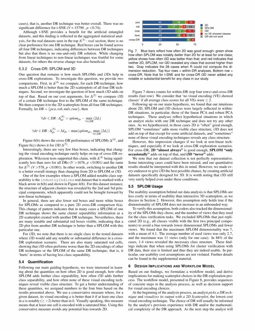
cases), that is, another DR technique was better overall. There was nosignificant difference for t-SNE (V = 15790 , p <0.74).

Although t-SNE provides a benefit for the artificial entangleddatasets, and this finding is reflected in the aggregated statistical anal-ysis, for the real datasets seen in the top ∆(3) : real section, there is noclear preference for one DR technique. Red boxes can be found acrossall four DR techniques, indicating differences between DR techniquesbut also that there is no one-and-only DR solution. While changingfrom linear techniques to non-linear techniques was fruitful for somedatasets, for others the reverse change was also beneficial.

5.3.2 Cross-DR: SPLOM and 3DOne question that remains is how much SPLOMs and i3Ds help incross-DR explorations. To investigate this question, we provide twocomparisons. First, in ∆(4) we compare, for each DR-technique, howmuch a SPLOM is better than the 2D scatterplots of all four DR tech-niques. Second, we investigate the question of how much i3D adds ontop of that. Based on our cost arguments, for ∆(5) we compare i3Dof a certain DR technique first to the SPLOM of the same technique.We then compare it to the 2D scatterplots from all four DR techniques.Formally, let DR = {pca,rob,mds, tsne}, then

∀dr ∈ DR : ∆(4)dr = splomdr− max

∀i∈DR(2di)

∀dr ∈ DR : ∆(5)dr = 3ddr−max(splomdr, max

∀i∈DR(2di))

Figure 6(b) shows the cross-DR performance of SPLOMs ∆(4), andFigure 6(c) shows it for i3D ∆(5).

Interestingly, there are very few blue boxes, indicating that chang-ing the visual encoding technique rarely helps on top of cross-DR ex-ploration. Wilcoxon tests supported this claim, with ∆(4) being signif-icantly less than zero for all DRs (V >1676, p <0.001) and the samefor ∆(5) (V >578, p <0.001). In other words, switching to another DRis a better overall strategy than changing from 2D to SPLOM or i3D.

One of the few examples where a SPLOM added notable class sep-arability is the industryIndices real dataset that is marked with ablack arrow in 6(b) and shown in Figure 4(b). For this dataset instance,the structure of adjacent clusters was revealed by the 2nd and 3rd prin-cipal components, which apparently could not be brought forward bynon-linear techniques.

In general, there are also fewer red boxes and more white boxesfor SPLOMs as compared to a pure 2D cross-DR comparison 6(a).This change of pattern indicates that in many cases a SPLOM of oneDR technique shows the same cluster separability information as a2D scatterplot created with another DR technique. Nevertheless, thereare many notable and substantial red boxes visible, indicating that a2D plot from another DR technique is better than a SPLOM with thisparticular one.

For i3D, we note that there is no single class in the tested datasetswhere i3D would add any notable or substantial difference in a cross-DR exploration scenario. There are also many saturated red cells,showing that i3D often performs worse than the 2D encodings of otherDR techniques or the SPLOM of the same DR technique; that is, it‘hurts’ in terms of having less class separability.

5.4 QuantificationFollowing our main guiding hypothesis, we were interested in learn-ing about the quantities on how often 2D is good enough, how oftenSPLOM adds further class separability, how often i3D adds furtherclass separability, and how often none of these visual encoding tech-niques reveal visible class structure. To get a better understanding ofthese quantities, we assigned numbers to the four bins based on theresults presented above. We use a conservative measure where, for agiven dataset, its visual encoding a is better than b if at least one classin a is notably (≥+2) better than in b. Visually speaking, this measuremeans that at least one cell is encoded with a saturated blue. Using thisconservative measure avoids any potential bias towards 2D.

pca rob mds tsne cross-DR2DSPLOM3DnothingDR not worked

43 36 47 49 6318 17 12 6 6

3 4 3 0 010 5 11 8 6

1 13 2 12 0

pca

rob

mds

tsne

cross-DR

0 25 50 75

2DSPLOMi3Dno VE showed classesDR did not work

43

364749

63

18

17126

6

3

43

10

511

8

13

12

6

1

2

Fig. 7. Blue bars reflect how often 2D was good enough; green showhow often SPLOM was notably better than 2D for at least for one class;yellow shows how often i3D was better than that; and red indicates thatneither 2D, SPLOM, nor i3D revealed any class that scored higher thantwo. Gray indicates the 28 cases when R could not compute the di-mension reduction. Top four rows = within-DR analyses, Bottom row =cross-DR. Note that for t-SNE and for cross-DR i3D never added anynotable or substantial benefit for any class in our study.

Figure 7 shows counts for within-DR (top four rows) and cross-DRresults (last row). We consider that ‘no visual encoding (VE) showedclasses’ if all average class scores for all VEs were ≤ 2.

Following up on our main hypothesis, we found that our intuitionsabout 2D, SPLOM and i3D choices were largely reflected in within-DR situations, in particular, those of the linear PCA and robust PCAtechniques. These analyses reflect hypothetical situations in whichan analyst sticks with one DR technique and does not try any otherones. As we hypothesized, in those cases 2D is “often” good enough,SPLOM “sometimes” adds more visible class structure, i3D does notadd on top of that except for some artificial datasets, and “sometimes”none of these visual encoding techniques reveals any class structure.

However, this impression changes if we look at non-linear tech-niques, and especially if we look at cross-DR exploration scenarios.For cross-DR, 2D “almost always” is good enough, SPLOM “onlyoccasionally” adds on top of that, and i3D “never” adds.

We note that our dataset collection is not perfectly representative.Some interesting cases could have been missed, and our quantitativeresults should be interpreted with this in mind. However, we made ev-ery endeavor to give i3D the best possible chance, by creating artificialdatasets specifically designed for 3D. It is worth noting that i3D stillvery rarely helped even under these conditions.

5.5 SPLOM UsageThe usability assumption behind our data analysis is that SPLOMs areless costly in terms of usability than interactive 3D scatterplots, as wediscuss in Section 2. However, this assumption only holds true if thedimensionality of SPLOM does not increase in an unbounded way.

To verify this assumption, both coders also tracked the dimensional-ity of the SPLOMs they chose, and the number of views that they usedfor the class verification tasks. We excluded SPLOMs that just repli-cated 2D (e.g., all classes visible with the first two principal compo-nents) to avoid a bias towards lower dimensional SPLOMs and fewerviews. We found that the maximum SPLOM dimensionality was 7,with a mean of 4.1. The average number of used views was only 2.7,and the maximum was 11 views (only for one case). In 88% of thecases, 1-4 views revealed the necessary class structure. These find-ings indicate that when using SPLOMs for cluster verification withDR data, their size is limited and thus they are indeed usable. In par-ticular, our usability cost assumptions are not violated. Further detailscan be found in the supplemental material.

6 DESIGN IMPLICATIONS AND WORKFLOW MODEL

Based on our findings, we formulate a workflow model, and deriveimplications for making scatterplot choices in the DR exploration pro-cess. The workflow model, presented in Figure 8, provides sequencesof concrete steps in the analysis process, as well as decision supportfor visual encoding choices.

At the beginning of the analysis process, an analyst picks a DR tech-nique and visualizes its output with a 2D Scatterplot, the lowest costvisual encoding technique. The choice of DR will usually be informedby the analyst’s previous experience with DR and/or the mathemati-cal complexity of the DR approach. As the next step the analyst will

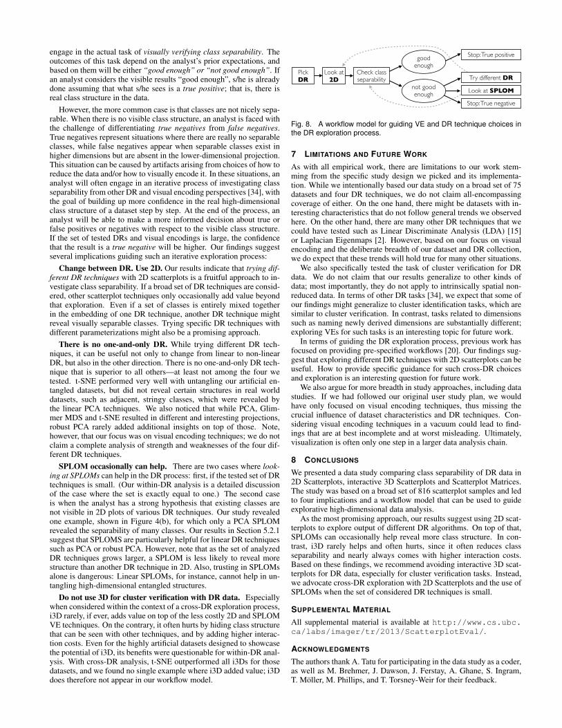
engage in the actual task of visually verifying class separability. Theoutcomes of this task depend on the analyst’s prior expectations, andbased on them will be either “good enough” or “not good enough”. Ifan analyst considers the visible results “good enough”, s/he is alreadydone assuming that what s/he sees is a true positive; that is, there isreal class structure in the data.

However, the more common case is that classes are not nicely sepa-rable. When there is no visible class structure, an analyst is faced withthe challenge of differentiating true negatives from false negatives.True negatives represent situations where there are really no separableclasses, while false negatives appear when separable classes exist inhigher dimensions but are absent in the lower-dimensional projection.This situation can be caused by artifacts arising from choices of how toreduce the data and/or how to visually encode it. In these situations, ananalyst will often engage in an iterative process of investigating classseparability from other DR and visual encoding perspectives [34], withthe goal of building up more confidence in the real high-dimensionalclass structure of a dataset step by step. At the end of the process, ananalyst will be able to make a more informed decision about true orfalse positives or negatives with respect to the visible class structure.If the set of tested DRs and visual encodings is large, the confidencethat the result is a true negative will be higher. Our findings suggestseveral implications guiding such an iterative exploration process:

Change between DR. Use 2D. Our results indicate that trying dif-ferent DR techniques with 2D scatterplots is a fruitful approach to in-vestigate class separability. If a broad set of DR techniques are consid-ered, other scatterplot techniques only occasionally add value beyondthat exploration. Even if a set of classes is entirely mixed togetherin the embedding of one DR technique, another DR technique mightreveal visually separable classes. Trying specific DR techniques withdifferent parameterizations might also be a promising approach.

There is no one-and-only DR. While trying different DR tech-niques, it can be useful not only to change from linear to non-linearDR, but also in the other direction. There is no one-and-only DR tech-nique that is superior to all others—at least not among the four wetested. t-SNE performed very well with untangling our artificial en-tangled datasets, but did not reveal certain structures in real worlddatasets, such as adjacent, stringy classes, which were revealed bythe linear PCA techniques. We also noticed that while PCA, Glim-mer MDS and t-SNE resulted in different and interesting projections,robust PCA rarely added additional insights on top of those. Note,however, that our focus was on visual encoding techniques; we do notclaim a complete analysis of strength and weaknesses of the four dif-ferent DR techniques.

SPLOM occasionally can help. There are two cases where look-ing at SPLOMs can help in the DR process: first, if the tested set of DRtechniques is small. (Our within-DR analysis is a detailed discussionof the case where the set is exactly equal to one.) The second caseis when the analyst has a strong hypothesis that existing classes arenot visible in 2D plots of various DR techniques. Our study revealedone example, shown in Figure 4(b), for which only a PCA SPLOMrevealed the separability of many classes. Our results in Section 5.2.1suggest that SPLOMS are particularly helpful for linear DR techniquessuch as PCA or robust PCA. However, note that as the set of analyzedDR techniques grows larger, a SPLOM is less likely to reveal morestructure than another DR technique in 2D. Also, trusting in SPLOMsalone is dangerous: Linear SPLOMs, for instance, cannot help in un-tangling high-dimensional entangled structures.

Do not use 3D for cluster verification with DR data. Especiallywhen considered within the context of a cross-DR exploration process,i3D rarely, if ever, adds value on top of the less costly 2D and SPLOMVE techniques. On the contrary, it often hurts by hiding class structurethat can be seen with other techniques, and by adding higher interac-tion costs. Even for the highly artificial datasets designed to showcasethe potential of i3D, its benefits were questionable for within-DR anal-ysis. With cross-DR analysis, t-SNE outperformed all i3Ds for thosedatasets, and we found no single example where i3D added value; i3Ddoes therefore not appear in our workflow model.

Look at SPLOM

Try different DR

Stop: True positive

Stop: True negative

Look at 2D

Pick DR

1

good enough

not good enough

Check class separability

Fig. 8. A workflow model for guiding VE and DR technique choices inthe DR exploration process.

7 LIMITATIONS AND FUTURE WORK

As with all empirical work, there are limitations to our work stem-ming from the specific study design we picked and its implementa-tion. While we intentionally based our data study on a broad set of 75datasets and four DR techniques, we do not claim all-encompassingcoverage of either. On the one hand, there might be datasets with in-teresting characteristics that do not follow general trends we observedhere. On the other hand, there are many other DR techniques that wecould have tested such as Linear Discriminate Analysis (LDA) [15]or Laplacian Eigenmaps [2]. However, based on our focus on visualencoding and the deliberate breadth of our dataset and DR collection,we do expect that these trends will hold true for many other situations.

We also specifically tested the task of cluster verification for DRdata. We do not claim that our results generalize to other kinds ofdata; most importantly, they do not apply to intrinsically spatial non-reduced data. In terms of other DR tasks [34], we expect that some ofour findings might generalize to cluster identification tasks, which aresimilar to cluster verification. In contrast, tasks related to dimensionssuch as naming newly derived dimensions are substantially different;exploring VEs for such tasks is an interesting topic for future work.

In terms of guiding the DR exploration process, previous work hasfocused on providing pre-specified workflows [20]. Our findings sug-gest that exploring different DR techniques with 2D scatterplots can beuseful. How to provide specific guidance for such cross-DR choicesand exploration is an interesting question for future work.

We also argue for more breadth in study approaches, including datastudies. If we had followed our original user study plan, we wouldhave only focused on visual encoding techniques, thus missing thecrucial influence of dataset characteristics and DR techniques. Con-sidering visual encoding techniques in a vacuum could lead to find-ings that are at best incomplete and at worst misleading. Ultimately,visualization is often only one step in a larger data analysis chain.

8 CONCLUSIONS

We presented a data study comparing class separability of DR data in2D Scatterplots, interactive 3D Scatterplots and Scatterplot Matrices.The study was based on a broad set of 816 scatterplot samples and ledto four implications and a workflow model that can be used to guideexplorative high-dimensional data analysis.

As the most promising approach, our results suggest using 2D scat-terplots to explore output of different DR algorithms. On top of that,SPLOMs can occasionally help reveal more class structure. In con-trast, i3D rarely helps and often hurts, since it often reduces classseparability and nearly always comes with higher interaction costs.Based on these findings, we recommend avoiding interactive 3D scat-terplots for DR data, especially for cluster verification tasks. Instead,we advocate cross-DR exploration with 2D Scatterplots and the use ofSPLOMs when the set of considered DR techniques is small.

SUPPLEMENTAL MATERIAL

All supplemental material is available at http://www.cs.ubc.ca/labs/imager/tr/2013/ScatterplotEval/.

ACKNOWLEDGMENTS

The authors thank A. Tatu for participating in the data study as a coder,as well as M. Brehmer, J. Dawson, J. Ferstay, A. Ghane, S. Ingram,T. Moller, M. Phillips, and T. Torsney-Weir for their feedback.

http://www.cs.ubc.ca/labs/imager/tr/2013/ScatterplotEval/

http://www.cs.ubc.ca/labs/imager/tr/2013/ScatterplotEval/

REFERENCES

[1] A. Anand, L. Wilkinson, and T. N. Dang. Visual Pattern Discovery usingRandom Projections. In Proc. IEEE Conf. Visual Analytics Science andTechnology (VAST), pages 43–52, 2012.

[2] M. Belkin and P. Niyogi. Laplacian eigenmaps and spectral techniquesfor embedding and clustering. Advances in neural information processingsystems, 14:585–591, 2001.

[3] E. Bertini and G. Santucci. Visual Quality Metrics. In Proc. AVI Work-shop on BEyond time and errors: novel evaluation methods for informa-tion visualization (BELIV). ACM, 2006.

[4] E. Bertini, A. Tatu, and D. A. Keim. Quality metrics in high-dimensionaldata visualization: an overview and systematization. IEEE Trans. on Vi-sualization and Computer Graphics (InfoVis), 17(12):2203–2212, 2011.

[5] I. Borg and P. Groenen. Modern multidimensional scaling: Theory andapplications. Springer, 2005.

[6] M. Chalmers. Using a landscape metaphor to represent a corpus of docu-ments. In Proc. European Conf. Spatial Information Theory (COSIT ’93),pages 377–390. Springer LNCS 716, 1993.

[7] K. Charmaz. Constructing grounded theory. A practical guide throughqualitative analysis. Sage Publications, Inc, 2006.

[8] A. Cockburn and B. McKenzie. An evaluation of cone trees. In Peopleand Computers XIV: Usability or Else. British Computer Society Conf. onHuman Computer Interaction, pages 425–436. Springer, 2000.

[9] A. Cockburn and B. McKenzie. 3D or not 3D?: evaluating the effectof the third dimension in a document management system. In Proc.ACM Conf. Human Factors in Computing Systems (CHI), pages 434–441,2001.

[10] A. Cockburn and B. McKenzie. Evaluating the effectiveness of spa-tial memory in 2D and 3D physical and virtual environments. In Proc.ACM Conf. Human Factors in Computing Systems (CHI), pages 203–210,2002.

[11] J. W. Creswell and V. L. P. Clark. Designing and conducting mixed meth-ods research. Wiley Online Library, 2007.

[12] I. Doyle, M. Ratcliffe, A. Walding, E. V. Bon, M. Dymond, W. Tomlin-son, D. Tilley, P. Shelton, and I. Dougall. Differential gene expressionanalysis in human monocyte-derived macrophages: impact of cigarettesmoke on host defence. Molecular immunology, 47(5):1058, 2010.

[13] A. L. Duran, J. Yang, L. Wang, and L. W. Sumner. Metabolomics spectralformatting, alignment and conversion tools (msfacts). Bioinformatics,19(17):2283–2293, 2003.

[14] S. Fabrikant. Spatial metaphors for browsing large data archives. PhDthesis, University of Colorado Boulder, 2000.

[15] R. A. Fisher. The use of multiple measurements in taxonomic problems.Annals of Human Genetics, 7(2):179–188, 1936.

[16] S. L. France and J. Carroll. Two-way multidimensional scaling: A re-view. IEEE Transactions on Systems, Man, and Cybernetics, Part C,41(5):644–661, 2011.

[17] A. Frank and A. Asuncion. University of California Irvine (UCI) MachineLearning Repository, 2010.

[18] D. Furniss, A. Blandford, and P. Curzon. Confessions from a GroundedTheory PhD: Experiences and Lessons Learnt. In ACM Trans. Computer-Human Interaction (ToCHI), pages 113–122, 2011.

[19] C. Holt and M. Bradford. Evaluating benchmarks of population statusfor Pacific salmon. North American Journal of Fisheries Management,31(2):363–378, 2011.

[20] S. Ingram, T. Munzner, V. Irvine, M. Tory, S. Bergner, and T. Moller.DimStiller: Workflows for dimensional analysis and reduction. In Proc.IEEE Conf. Visual Analytics Science and Technology (VAST), 2010.

[21] S. Ingram, T. Munzner, and M. Olano. Glimmer: Multilevel MDS onthe GPU. IEEE Trans. Visualization and Computer Graphics (TVCG),15(2):249–261, 2009.

[22] I. T. Jolliffe. Principal Component Analysis, 2nd ed. Springer, 2002.[23] H. S. Kim, J. P. Schulze, A. C. Cone, G. E. Sosinsky, and M. E. Mar-

tone. Dimensionality reduction on multi-dimensional transfer functionsfor multi-channel volume data sets. Information visualization, 9(3):167–180, 2010.

[24] K. Krippendorff. Content Analysis: An Introduction to Its Methodology.Sage, 2004.

[25] J. Kruskal and M. Wish. Multidimensional Scaling. Sage, 1978.[26] H. Lam. A framework of interaction costs in information visualization.

IEEE Trans. Visualization and Computer Graphics (InfoVis), 14(6):1149–1156, 2008.

[27] J. M. Lewis, M. Ackerman, and V. de Sa. Human cluster evaluation andformal quality measures: A comparative study. In Proc. 34th Conf. of theCognitive Science Society (CogSci), pages 1870–1875, 2012.

[28] J. M. Lewis, L. van der Maaten, and V. de Sa. A behavioral investigationof dimensionality reduction. In Proc. 34th Conf. of the Cognitive ScienceSociety (CogSci), pages 671–676, 2012.

[29] J. Li, J.-B. Martens, and J. J. van Wijk. Judging correlation from scatter-plots and parallel coordinate plots. Information Visualization, 9(1):13–30,2008.

[30] G. Newby. Empirical study of a 3D visualization for information retrievaltasks. J. Intelligent Information Systems, 18(1):31–53, 2002.

[31] R. Rensink and G. Baldridge. The perception of correlation in scatter-plots. Computer Graphics Forum (EuroVis), 29(3):1203–1210, 2010.

[32] T. Sando, M. Tory, and P. Irani. Effects of animation, user-controlledinteractions, and multiple static views in understanding 3d structures. InProc. Symp. Applied Perception in Graphics and Visualization (APGV),pages 69–76, 2009.

[33] SAP. HANA, 2010. http://www.sap.com/hana/, last accessed 01/10.[34] M. Sedlmair, M. Brehmer, S. Ingram, and T. Munzner. Dimensionality

reduction in the wild: Gaps and guidance. Technical report, Dept. ofComputer Science, University of British Columbia, 2012.

[35] M. Sedlmair, A. Tatu, M. Tory, and T. Munzner. A taxonomy of vi-sual cluster separation factors. Computer Graphics Forum (EuroVis),31(3):1335–1344, 2012.

[36] M. Sips, B. Neubert, J. P. Lewis, and P. Hanrahan. Selecting good viewsof high-dimensional data using class consistency. Computer GraphicsForum (EuroVis), 28(3):831–838, 2009.

[37] M. St. John, M. B. Cowen, H. S. Smallman, and H. M. Oonk. The useof 2-D and 3-D displays for shape understanding versus relative positiontasks. Human Factors, 43(1):79–98, 2001.

[38] A. Tatu, G. Albuquerque, M. Eisemann, J. Schneidewind, H. Theisel,M. Magnor, and D. Keim. Combining automated analysis and visu-alization techniques for effective exploration of high-dimensional data.In Proc. IEEE Symp. Visual Analytics Science and Technology (VAST),pages 59–66, 2009.

[39] V. Todorov and P. Filzmoser. An object oriented framework for robustmultivariate analysis. Journal of Statistical Software, 32(3):1–47, 2009.

[40] M. Tory, D. Sprague, F. Wu, W. Y. So, and T. Munzner. Spatializationdesign: comparing points and landscapes. IEEE Trans. on Visualizationand Computer Graphics (InfoVis), 13(6):1262–9, 2007.

[41] M. Tory, C. Swindells, and R. Dreezer. Comparing dot and landscape spa-tializations for visual memory differences. IEEE Trans. on Visualizationand Computer Graphics (InfoVis), 15(6):1033–9, 2009.

[42] University of Massachusetts. Statistical Data and Software Help, 2011.http://www.umass.edu/statdata/statdata/, last accessed 11/11.

[43] L. van der Maaten. Learning a parametric embedding by preserving localstructure. Proc. Int. Conf. on Artificial Intelligence and Statistics (AI-STATS), 5:384–391, 2009.

[44] L. van der Maaten and G. Hinton. Visualizing data using t-SNE. Journalof Machine Learning Research, 9(2579-2605):85, 2008.

[45] L. Van der Maaten, E. Postma, and H. Van Den Herik. Dimensionalityreduction: A comparative review. Journal of Machine Learning Research,10:1–41, 2009.

[46] J. J. van Wijk. Views on visualization. IEEE Trans. Visualization andComputer Graphics (TVCG), 12(2):421–432, 2006.

[47] VisuMap Technologies Inc. VisuMap Data Repository, 2011.http://www.visumap.net/, last accessed 11/11.

[48] M. O. Ward. Xmdv data repository, 2011.http://davis.wpi.edu/xmdv/datasets.html, last accessed 11/11.

[49] C. Ware. Designing with a 2 1/2 D Attitude. Information Design Journal,10(3):255–262, 2001.

[50] S. Westerman. Browsing a document collection represented in two- andthree-dimensional virtual information space. Intl. Journal Human Com-puter Studies (IJHCS), 62(6):713–736, 2005.

[51] S. Westerman and T. Cribbin. Mapping semantic information in virtualspace: dimensions, variance and individual differences. Intl. Journal Hu-man Computer Studies (IJHCS), 53(5):765–787, 2000.

[52] C. Wickens and E. Merwin, D.H.and Lin. Implications of graphics en-hancements for the visualization of scientific data: Dimensional integral-ity, stereopsis, motion, and mesh. Human Factors, 36(1):44–61, 1994.

[53] L. Wilkinson and A. Anand. Graph-theoretic scagnostics. Proc. IEEESymp. Information Visualization (InfoVis), pages 157–164, 2005.

empirical guidance on scatterplot and dimension reduction ... · 2 2d, 3d, splom: justifications...

Documents