empirical methods of linguistics research - …x4diho/script empirical methods... · 2007-10-17 ·...

1

Empirical Methods of Linguistics

ResearchScript WS 2007/8

Holger Diessel

Criteria for empirical research

a. Objectivityb. Reliabilityc. Internally validityd. Externally validitye. Occam’s Razor

Stages of an empirical investigation

1. Exploration phasea. Literature researchb. Impressionistic analysis of observational datac. Informal pretest

2. Theoretical phasea. State your hypotheses (informally)b. Are your hypotheses falsifiable?c. Are your hypotheses compatible with your theoretical framework?

3. Planning phasea. Select a methodb. Define and operationalize the variablesc. Select the appropriate statistical measure

4. Data collectionData collection has to follow a predetermined procedure. Don’t change the procedure in the middle of your study.

5. Analysis and decisiona. Describe the frequency datab. Submit the frequency data to statistical analysis

2

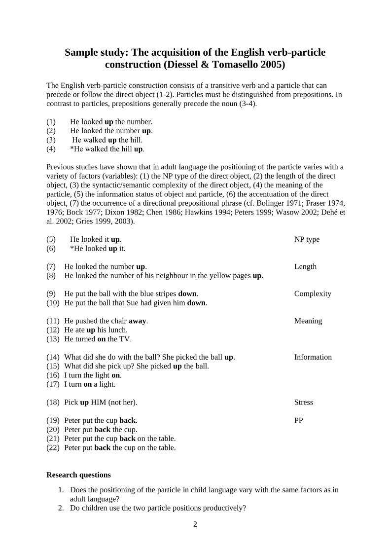
Sample study: The acquisition of the English verb-particle construction (Diessel & Tomasello 2005)

The English verb-particle construction consists of a transitive verb and a particle that can precede or follow the direct object (1-2). Particles must be distinguished from prepositions. In contrast to particles, prepositions generally precede the noun (3-4).

(1) He looked up the number.(2) He looked the number up.(3) He walked up the hill.(4) *He walked the hill up.

Previous studies have shown that in adult language the positioning of the particle varies with a variety of factors (variables): (1) the NP type of the direct object, (2) the length of the direct object, (3) the syntactic/semantic complexity of the direct object, (4) the meaning of the particle, (5) the information status of object and particle, (6) the accentuation of the direct object, (7) the occurrence of a directional prepositional phrase (cf. Bolinger 1971; Fraser 1974, 1976; Bock 1977; Dixon 1982; Chen 1986; Hawkins 1994; Peters 1999; Wasow 2002; Dehé et al. 2002; Gries 1999, 2003).

(5) He looked it up. NP type(6) *He looked up it.

(7) He looked the number up. Length(8) He looked the number of his neighbour in the yellow pages up.

(9) He put the ball with the blue stripes down. Complexity(10) He put the ball that Sue had given him down.

(11) He pushed the chair away. Meaning(12) He ate up his lunch.(13) He turned on the TV.

(14) What did she do with the ball? She picked the ball up. Information(15) What did she pick up? She picked up the ball.(16) I turn the light on.(17) I turn on a light.

(18) Pick up HIM (not her). Stress

(19) Peter put the cup back. PP(20) Peter put back the cup. (21) Peter put the cup back on the table.(22) Peter put back the cup on the table.

Research questions

1. Does the positioning of the particle in child language vary with the same factors as in adult language?

2. Do children use the two particle positions productively?

3

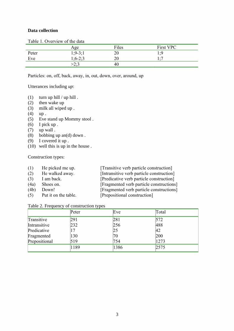
Data collection

Table 1. Overview of the dataAge Files First VPC

PeterEve

1;9-3;11;6-2;3

2020

1;91;7

>2;3 40

Particles: on, off, back, away, in, out, down, over, around, up

Utterances including up:

(1) turn up hill / up hill .(2) then wake up(3) milk all wiped up .(4) up .(5) Eve stand up Mommy stool .(6) I pick up .(7) up wall .(8) bobbing up an(d) down .(9) I covered it up .(10) well this is up in the house .

Construction types:

(1) He picked me up. [Transitive verb particle construction](2) He walked away. [Intransitive verb particle construction](3) I am back. [Predicative verb particle construction](4a) Shoes on. [Fragmented verb particle constructions](4b) Down! [Fragmented verb particle constructions](5) Put it on the table. [Prepositional construction]

Table 2. Frequency of construction typesPeter Eve Total

TransitiveIntransitivePredicativeFragmentedPrepositional

291 232 17 130 519

281256 25 70 754

572488422001273

1189 1386 2575

4

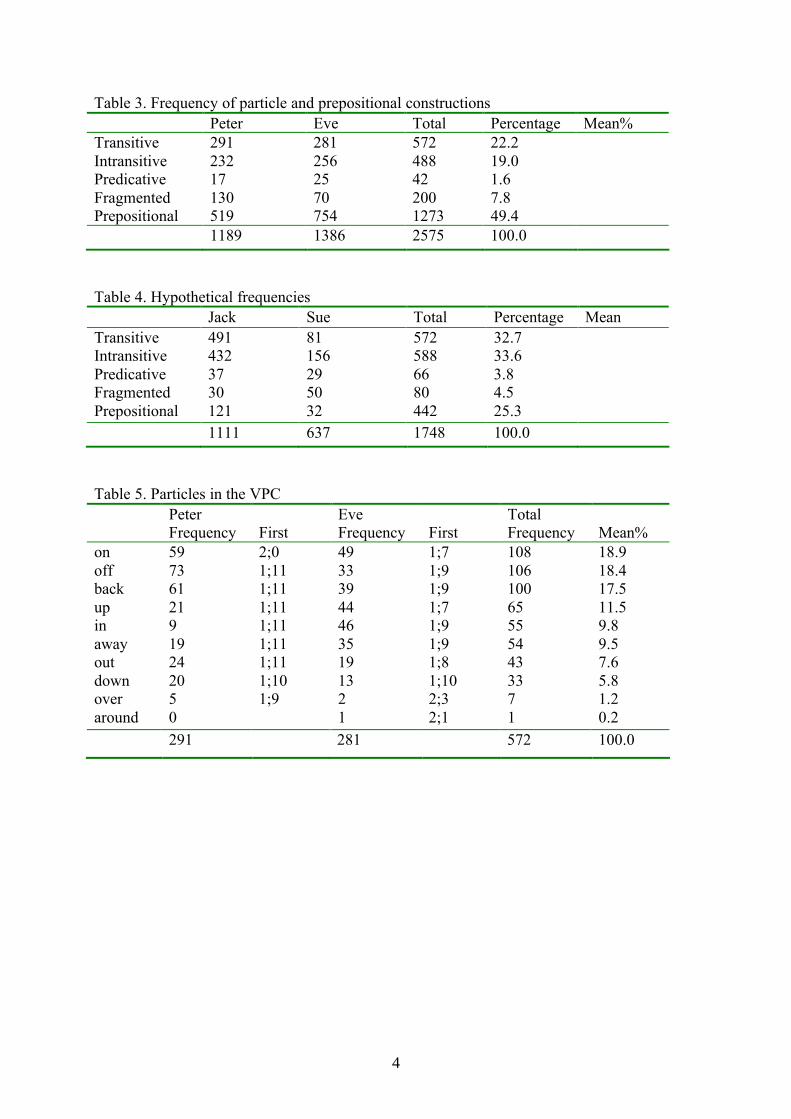
Table 3. Frequency of particle and prepositional constructions Peter Eve Total Percentage Mean%


29123217130519

2812562570754

572488422001273

22.219.01.67.849.4

1189 1386 2575 100.0

Table 4. Hypothetical frequencies Jack Sue Total Percentage Mean


4914323730121

81156295032

5725886680442

32.733.63.84.525.3

1111 637 1748 100.0

Table 5. Particles in the VPCPeterFrequency First

EveFrequency First

TotalFrequency Mean%

onoffbackupinawayoutdownoveraround

59736121919242050

2;01;111;111;111;111;111;111;101;9–

493339444635191321

1;71;91;91;71;91;91;81;102;32;1

108106100655554433371

18.918.417.511.59.89.57.65.81.20.2

291 281 572 100.0

5

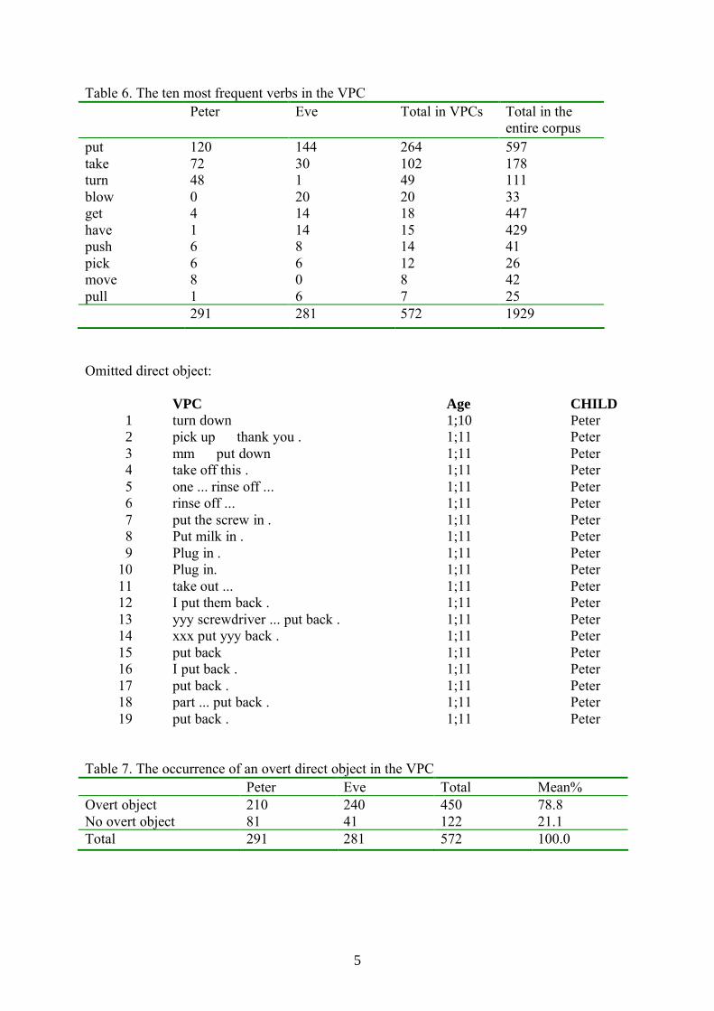
Table 6. The ten most frequent verbs in the VPCPeter Eve Total in VPCs Total in the

entire corpusputtaketurnblowgethavepushpickmovepull

12072480416681

1443012014148606

26410249201815141287

5971781113344742941264225

291 281 572 1929

Omitted direct object:

VPC Age CHILD1 turn down 1;10 Peter2 pick up … thank you . 1;11 Peter3 mm … put down … 1;11 Peter4 take off this . 1;11 Peter5 one ... rinse off ... 1;11 Peter6 rinse off ... 1;11 Peter7 put the screw in . 1;11 Peter8 Put milk in . 1;11 Peter9 Plug in . 1;11 Peter

10 Plug in. 1;11 Peter11 take out ... 1;11 Peter12 I put them back . 1;11 Peter13 yyy screwdriver ... put back . 1;11 Peter14 xxx put yyy back . 1;11 Peter15 put back 1;11 Peter16 I put back . 1;11 Peter17 put back . 1;11 Peter18 part ... put back . 1;11 Peter19 put back . 1;11 Peter

Table 7. The occurrence of an overt direct object in the VPC Peter Eve Total Mean%

Overt objectNo overt object

21081

24041

450122

78.821.1

Total 291 281 572 100.0

6

Coding

Spalte1 Construction Lenght Complexity Definiteness Meaning1 take off this .2 put the screw in .3 Put milk in .4 I put them back .5 put em back ... ok .6 turn it over .7 turn it over .8 turn on a light off .9 ... turn on a light off .

10 pick up my cup .11 take off wheels .12 telephone ... put back ... telephone .13 pick am up .14 close it up .15 close it … up .16 I turn the light on .17 turn it on … 18 turn it on … xxx .19 uhhuh … we have to put our coats on.20 take this … put it on .21 my put barrette on .22 a turn on a light !23 turn it on … 24 there put it on .25 right there … turn the light on .26 put it on … .27 a put it on … 28 my put it on .29 ...... got engine off .30 don't take a wheels off ... 31 turn it off ... there .32 I turn that off .33 push it off ... 34 get your hand off .35 take it out .36 take a out .37 turn a light out ... xxx .38 let’s take a piece out .39 put it back .40 put a back .41 I put the pen back in my pocketbook .42 put more back .43 my out put ... xxx ... put more back ....44 in a box ... gonna put a back too .45 put it back .46 let's put it back right there .47 ... put xxx away ....48 put these away .49 put toys away ... go home ... 50 turn it over ?51 a turn it over ... uhoh .52 all finished put it on a tape recorder on.53 I do it … turn on the light on .

7

Coding scheme

Column Category Values ExampleA CHILD 1 = Peter

2 = EveB CONSTRUCTIO 1 = V NP P

2 = V P NPLook the number upLook up the number

C LENGTH 1 = 1 word2 = 2 words3 = 3+ words

Pick it upPick the ball upPick the blue ball up

D COMPLEXITY 0 = simple1 = intermediate2 = complex

Pick it up [PRO, (ART)-N]Pick my ball up [GEN-N, N-PP, N and N]Pick up the one I want [N-CLAUSE]

E DEFINITENESS 0 = no determiner1 = def. determiner2 = indef. determin

Pick book up [PRO, bare N]Pick the ball up [the, my, this, etc.]Pick a ball up [a]

F NP-Type 1 = unstressed PRO2 = stressed PRO3 = lexical

Pick it upPick this upPick the ball up

G MEANING 0 = spatial1 = non-spatial

Pick me upEat it up

H PP 0 = no PP1 = PP

Put it back on the floorPut it back

I PARTICLE 1 = up2 = down3 = on4 = off5 = in6 = out7 = back8 = away9 = over0 = around

Pick it upPut it downPut it onPut it offPut in itTake it outPut it backPut it awayTurn it overTurn it around

Results

Table 1. Frequency of the different particle positions in the VPCPeter Eve Total Mean%

V NP PV P NP

19515

22614

29421

93.56.5

210 240 572 100.0

8

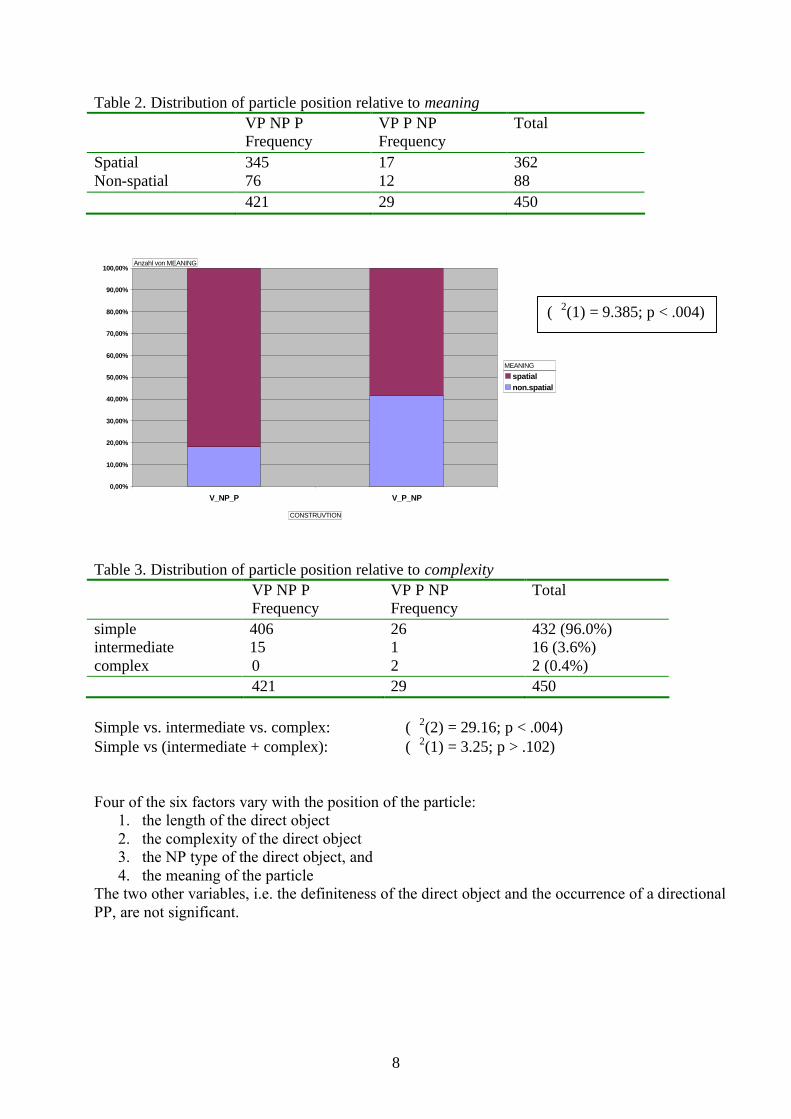
Table 2. Distribution of particle position relative to meaningVP NP PFrequency

VP P NPFrequency

Total

SpatialNon-spatial

34576

1712

36288

421 29 450

0,00%

10,00%

20,00%

30,00%

40,00%

50,00%

60,00%

70,00%

80,00%

90,00%

100,00%

V_NP_P V_P_NP

spatialnon.spatial

Anzahl von MEANING

CONSTRUVTION

MEANING

Table 3. Distribution of particle position relative to complexityVP NP PFrequency

VP P NPFrequency

Total

simpleintermediatecomplex

406150

2612

432 (96.0%)16 (3.6%)2 (0.4%)

421 29 450

Simple vs. intermediate vs. complex: (2(2) = 29.16; p < .004) Simple vs (intermediate + complex): (2(1) = 3.25; p > .102)

Four of the six factors vary with the position of the particle: 1. the length of the direct object2. the complexity of the direct object3. the NP type of the direct object, and 4. the meaning of the particle

The two other variables, i.e. the definiteness of the direct object and the occurrence of a directional PP, are not significant.

(2(1) = 9.385; p < .004)

9

Multifactorial analysis: Logistic regression

Table 1. Result of the logistic regression Factor Odds ratio p value

NP type

Meaning

lexical Ns vs. personal PROsother PROs vs. personal PROslexical Ns vs. other PROSspatial vs. non-spatial

= 72.46= 22.04= 3.29= 7.1

.001

.029

.156

.001

Discussion

Hypothesis 1:Children as young as 2,0 years of age process the verb-particle construction in the same way as adult speakers (except maybe that they do not take all factors into account).

Hypothesis 2:Children ‘re-produce’ the verb-particle constructions they encounter in the ambient language without processing the factors that influence particle placement in adult language.

complexity

length

meaning

NP type

PP

definiteness

V_NP_P

V_P_NP

10

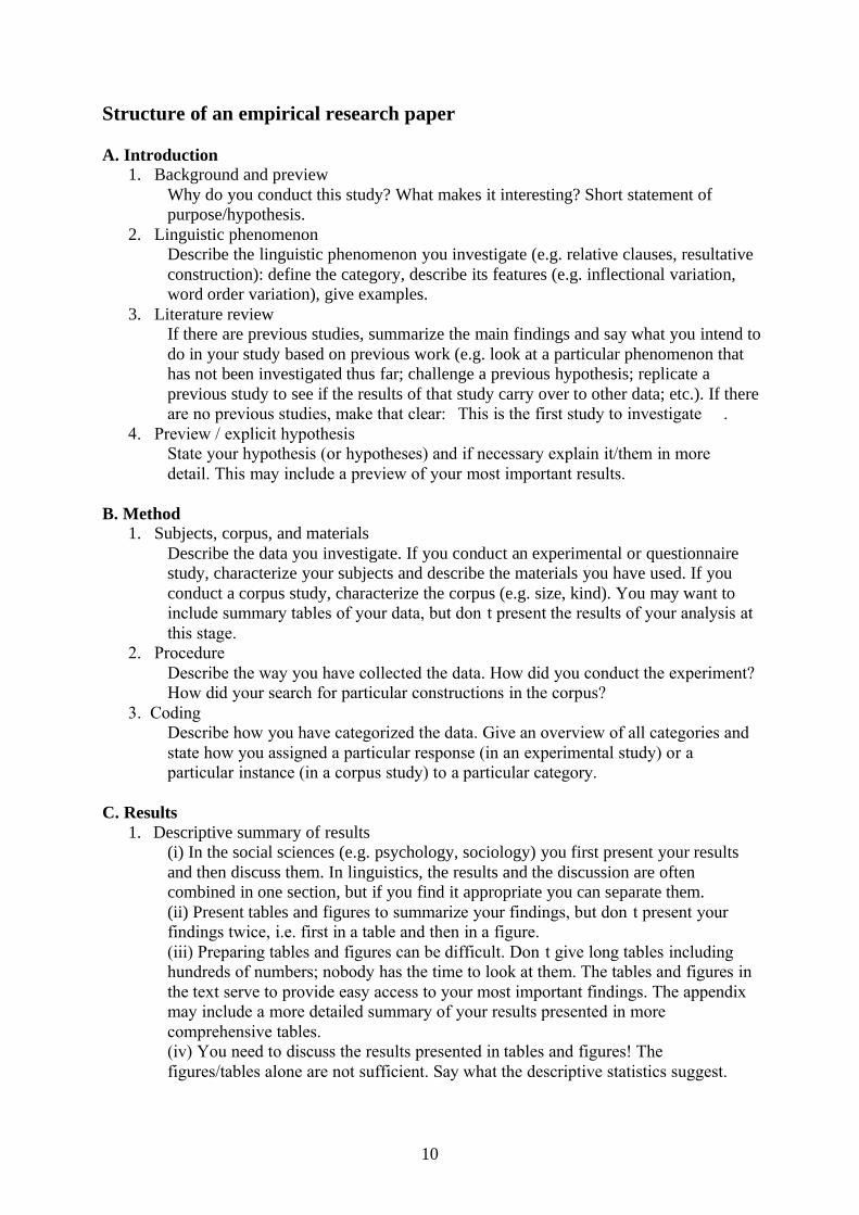
Structure of an empirical research paper

A. Introduction1. Background and preview

Why do you conduct this study? What makes it interesting? Short statement of purpose/hypothesis.

2. Linguistic phenomenonDescribe the linguistic phenomenon you investigate (e.g. relative clauses, resultative construction): define the category, describe its features (e.g. inflectional variation, word order variation), give examples.

3. Literature reviewIf there are previous studies, summarize the main findings and say what you intend to do in your study based on previous work (e.g. look at a particular phenomenon that has not been investigated thus far; challenge a previous hypothesis; replicate a previous study to see if the results of that study carry over to other data; etc.). If there are no previous studies, make that clear: “This is the first study to investigate ….”

4. Preview / explicit hypothesisState your hypothesis (or hypotheses) and if necessary explain it/them in more detail. This may include a preview of your most important results.

B. Method1. Subjects, corpus, and materials

Describe the data you investigate. If you conduct an experimental or questionnaire study, characterize your subjects and describe the materials you have used. If you conduct a corpus study, characterize the corpus (e.g. size, kind). You may want to include summary tables of your data, but don’t present the results of your analysis at this stage.

2. ProcedureDescribe the way you have collected the data. How did you conduct the experiment? How did your search for particular constructions in the corpus?

3. CodingDescribe how you have categorized the data. Give an overview of all categories and state how you assigned a particular response (in an experimental study) or a particular instance (in a corpus study) to a particular category.

C. Results1. Descriptive summary of results

(i) In the social sciences (e.g. psychology, sociology) you first present your results and then discuss them. In linguistics, the results and the discussion are often combined in one section, but if you find it appropriate you can separate them.(ii) Present tables and figures to summarize your findings, but don’t present your findings twice, i.e. first in a table and then in a figure.(iii) Preparing tables and figures can be difficult. Don’t give long tables including hundreds of numbers; nobody has the time to look at them. The tables and figures in the text serve to provide easy access to your most important findings. The appendix may include a more detailed summary of your results presented in more comprehensive tables. (iv) You need to discuss the results presented in tables and figures! The figures/tables alone are not sufficient. Say what the descriptive statistics suggest.

11

2. Inferential statisticsOnce you have described your data, submit them to statistical analysis. Say what type of test you have used and present the relevant measures (e.g. p-value, F-value, degrees of freedom, effect size, confidence intervals). If it is not obvious, why you used a particular test, explain your decision, but don’t describe obvious choices (e.g. I have used a chi-square test because the data is frequency data). Say also what the statistical analysis suggests, i.e. how the result should be interpreted.

D. Discussion1. Provide a short summary of your results2. Theoretical implications: If possible consider your paper from a broader theoretical

perspective and mention implications of your study for related questions.4. Future direction of research: Mention open questions: What should be done in the next

step? Ideas for an experiment. Etc.

AppendixIf the data are too comprehensive to be included in the text, include them in the appendix. If the data are very comprehensive, you might only present parts of your data in the appendix.

ReferencesList all articles and books you have cited.

12

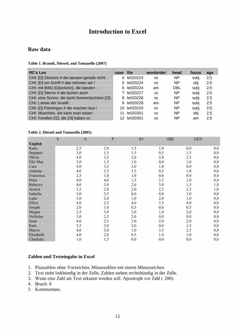
Introduction to Excel

Raw data

Table 1. Brandt, Diessel, and Tomasello (2007)

RC's Leo case file wordorder head focus ageCHI: [D] Glocken # die laeuten gerade nicht . 4 le020223 vs NP subj 2;5CHI: [D] ein Schiff # das nehmen wir ! 5 le020224 vs NP obj 2;5CHI: mit [MA] (G)locke(n), die laeuten . 6 le020224 am OBL subj 2;5CHI: [D] Sterne # die lachen auch . 7 le020227 vs NP subj 2;5CHI: eine Sonne, die lacht Sonnen(sch)ein [/2]. 8 le020228 vs NP subj 2;5CHI: Loewe der bruellt . 9 le020228 am NP subj 2;5CHI: [D] Flamingos # die machen laut ! 10 le020229 vs NP subj 2;5CHI: Muscheln, die kann man essen . 11 le020301 vs NP obj 2;5CHI: Forellen [/2], die [/3] haben xx . 12 le020301 vs NP am 2;5

Table 2. Diessel and Tomasello (2005)

EnglishS A P IO OBL GEN

Katie 2,5 2,0 1,5 1,0 0,0 0,0Stepanie 3,0 1,5 1,5 0,5 1,5 0,0Olivia 4,0 3,5 2,0 2,0 2,5 0,0Elle Mae 3,0 1,5 1,0 0,0 1,0 0,0Cara 4,0 3,5 2,0 1,0 0,0 0,0Antonia 4,0 2,5 3,5 0,5 1,0 0,0Francesca 2,5 1,0 1,0 0,0 0,0 0,0Peter 4,0 4,0 1,5 2,5 1,0 0,0Rebecca 4,0 3,0 2,0 3,0 1,5 1,0Jessica 3,5 2,0 2,0 2,5 2,5 1,0Isabella 3,0 3,5 0,0 0,0 1,0 0,0Luke 3,0 2,0 1,0 2,0 1,0 0,0Elliot 4,0 2,5 4,0 3,5 4,0 0,0Joseph 2,0 1,0 0,5 0,0 0,5 0,0Megan 3,5 3,0 2,0 1,0 2,0 0,0Nicholas 3,0 2,5 2,0 0,0 0,0 0,0Sean 4,0 2,5 3,0 2,0 2,0 0,0Kate 3,5 2,0 2,0 0,0 1,5 0,0Maeve 4,0 3,0 1,0 3,5 2,5 0,0Elizabeth 4,0 2,0 0,5 1,0 1,0 0,0Charlotte 1,0 1,5 0,0 0,0 0,0 0,0

Zahlen und Texteingabe in Excel

1. Pluszahlen ohne Vorzeichen; Minuszahlen mit einem Minuszeichen.2. Text steht linkbündig in der Zelle, Zahlen stehen rechtsbündig in der Zelle.3. Wenn eine Zahl als Text erkannt werden soll: Apostroph vor Zahl (’200).4. Bruch: 0 ¾ 5. Kommentare.

13

Funktionen Daten sortieren Taschenrechnerfunktionen Funktionsassistent

Pivot-Bericht

Aufgabe 1 (Daten: Gries 2003)1. Erstellen Sie eine Graphik, die die Anzahl von belebten und unbelebten Objekten in

den beiden Konstruktionen zeigt.2. Erstellen Sie eine Graphik, die den prozentualen Anteil von lexikalischen,

pronominalen, semi-pronominalen, und Eigennamen in den beiden Konstruktionen zeigt.

3. Erstellen Sie eine Graphik, die die mittlere Länge der Objekte in den beiden Konstruktionen zeigt.

Aufgabe 2 (Daten: Brandt, Diessel, and Tomasello in press)Head(1) Der Mann, den ich gesehen habe, war blond.(2) Peter sieht den Jungen, mit dem ich gesprochen habe.(3) Peter sitzt auf dem Stuhl, auf dem ich gestern gesessen habe.(4) Das ist der Junge, der mir die Tür aufgemacht hat.(5) Das Bild, das ich gemalt habe.Focus(1) Der Mann, der mich gesehen hat.(2) Der Mann, den ich gesehen habe.(3) Der Mann, mit dem ich gesprochen habe.

Word order Head focus Agevf (verb final)vs (verb second)am (ambiguous)

SUBJOBJOBLPNNP

subjobjoblam

2;53;03;54;04;5

1. Erstellen Sie ein Liniendiagramm, das die Entwicklung der beiden Wortstellungskonstruktionen zeigt.

2. Erstellen Sie ein Säulendiagramm, das die Anzahl der verschiedenen Relativsatzarten (Focus) im Gesamtkorpus zeigt.

3. Erstellen Sie ein Säulendiagramm, das den prozentualen Anteil der Foci in den beiden Wortstellungskonstruktionen zeigt.

Aufgaben 3 (Daten: Brandt, Diessel, and Tomasello in press)1. Erstellen Sie ein Säulendiagramm, das den Anteil der verschiedenen Köpfe im

Gesamtkorpus zeigt.2. Erstellen Sie ein Liniendiagramm, das die Entwicklung der verschiedenen Köpfe in

den verschiedenen Alterstufen zeigt.3. Erstellen Sie ein Säulendiagramm, das den prozentualen Anteil der Köpfe in den

beiden Wortstellungskonstruktionen zeigt.Lassen Sie in allen Graphiken die Variablenausprägung ‘am’ unberücksichtigt.

14

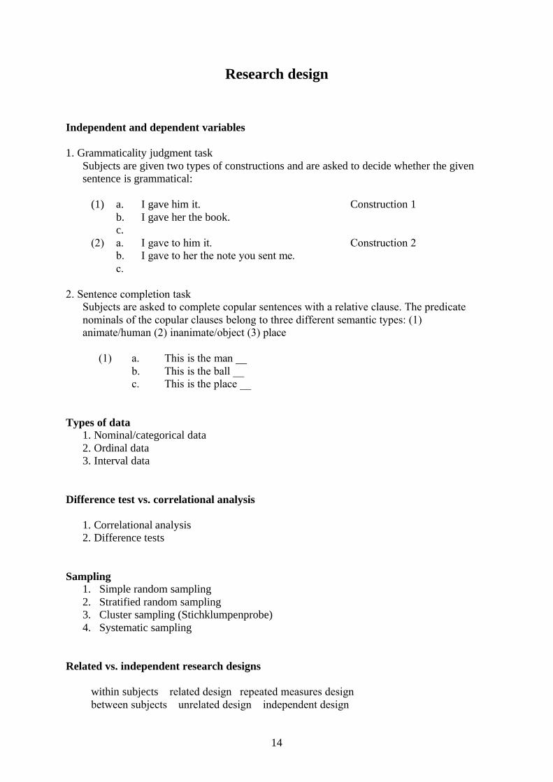
Research design

Independent and dependent variables

1. Grammaticality judgment taskSubjects are given two types of constructions and are asked to decide whether the given sentence is grammatical:

(1) a. I gave him it. Construction 1b. I gave her the book.c. …

(2) a. I gave to him it. Construction 2b. I gave to her the note you sent me.c. …

2. Sentence completion taskSubjects are asked to complete copular sentences with a relative clause. The predicate nominals of the copular clauses belong to three different semantic types: (1) animate/human (2) inanimate/object (3) place

(1) a. This is the man __ b. This is the ball __c. This is the place __

Types of data1. Nominal/categorical data2. Ordinal data3. Interval data

Difference test vs. correlational analysis

1. Correlational analysis2. Difference tests

Sampling1. Simple random sampling2. Stratified random sampling3. Cluster sampling (Stichklumpenprobe)4. Systematic sampling

Related vs. independent research designs

within subjects – related design –repeated measures designbetween subjects – unrelated design – independent design

15

Experimental design

A child language researcher wants to find out if the acquisition of relative clauses is affected by its syntactic structure. The structure of a relative clause is defined by two features: The syntactic function of the head, i.e. the main clause element that is modified by a relative clause, and the syntactic function of the gap, i.e. the element in the relative clause that is omitted. As can be seen in examples (1) to (4), both head and gap can function as subject or object.

(1) Peter saw the man who talked to Sally last night. OS(2) Jack noticed the man who Sally met yesterday. OO(3) The man who talked to Sally last night saw Peter. SS(4) The man who Sally met yesterday noticed Jack. SO

A very simple, but frequently used experimental method to test children’s comprehension of linguistic structures is the sentence repetition task, in which children have to repeat a linguistic structure they may find difficult to understand. If a child is not able to understand the structure, s/he is not able to repeat it. Nobody, neither children nor adults, are able to memorize more than 7 randomly combined words. In order to memorize and repeat longer word sequences, the sequence must make sense, i.e. you must be able to understand it. If you are not able to understand it, you either don’t respond or you change the given structure to a structure you understand.

Table 1. Schematic token setHeadschematic token set

SUBJ OBJSUBJ a (s+s) b (s+b)Gap OBJ c (b+s) d (b+b)

Table 2. Concrete token setsHEAD

token set 1 subject objectSUBJ The man who met Sally talked to me. I talked to the man who met Sally.

REL PRO OBJ The man who Sally met talked to me. I talked to the man who Sally met.

HEADtoken set 2 subject object

SUBJ The girl who saw Jack kissed Bill. Bill saw the girl who kissed Jack.REL PRO OBJ The girl who Jack saw kissed Bill. Bill saw the girl who Jack kissed.


SUBJ The cat that chased the dog scared the horse. The cat chased the dog that scared the horse.REL PRO OBJ The cat that the dog chased scared the horse. The cat chased the dog that the horse scared.


SUBJ The car that hit the bus pumped into the van. The car hit the bus that pumped into the van.REL PRO OBJ The car that the bus hit pumped into the van. The car hit the bus that pumped into the van.

16

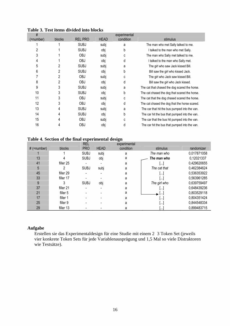
Table 3. Test items divided into blocks#

(=number) blocks REL PRO HEADexperimental

condition stimulus1 1 SUBJ subj a The man who met Sally talked to me.2 1 SUBJ obj b I talked to the man who met Sally.3 1 OBJ subj c The man who Sally met talked to me.4 1 OBJ obj d I talked to the man who Sally met.5 2 SUBJ subj a The girl who saw Jack kissed Bill.6 2 SUBJ obj b Bill saw the girl who kissed Jack.7 2 OBJ subj c The girl who Jack saw kissed Bill.8 2 OBJ obj d Bill saw the girl who Jack kissed.9 3 SUBJ subj a The cat that chased the dog scared the horse.

10 3 SUBJ obj b The cat chased the dog that scared the horse.11 3 OBJ subj c The cat that the dog chased scared the horse.12 3 OBJ obj d The cat chased the dog that the horse scared.13 4 SUBJ subj a The car that hit the bus pumped into the van.14 4 SUBJ obj b The car hit the bus that pumped into the van.15 4 OBJ subj c The car that the bus hit pumped into the van.16 4 OBJ obj d The car hit the bus that pumped into the van.

Table 4. Section of the final experimental design

# (=number) blocksREL PRO HEAD

experimental condition stimulus randomizer

1 1 SUBJ subj a The man who … 0,01787105813 4 SUBJ obj a The man who … 0,1202133741 filler 25 - - a [...] 0,4296206555 2 SUBJ subj a The cat that … 0,462384624

45 filler 29 - - a [...] 0,53635392233 filler 17 - - a [...] 0,5639612859 3 SUBJ obj a The girl who … 0,639759497

37 filler 21 - - a [...] 0,64843923621 filler 5 - - a [...] 0,80352911817 filler 1 - - a [...] 0,80435142425 filler 9 - - a [...] 0,84454833429 filler 13 - - a [...] 0,899483715

AufgabeErstellen sie das Experimentaldesign für eine Studie mit einem 23 Token Set (jeweils vier konkrete Token Sets für jede Variablenausprägung und 1,5 Mal so viele Distraktoren wie Testsätze).

17

Mean and variance

Central tendency

Data: 2,3,3,3,4,6,6,9,12,13,13

1. Mean(2+3+3+3+4+6+6+9+12+13+13)/11 = 6.72

2. MedianThe middle score (i.e. 6). If there is no data value that represents the middle score, you add the two closest data points and divide them by 2.

3. ModeThe most frequent score (i.e. 3).

Variance and standard deviation

Exercise: Determine the mean number of words and their variation.

S words (=X1 – Xmean) d1 d12 (residuals)

12345678

3749129114

3 – 7.4 7 – 7.44 – 7.49 – 7.412 – 7.49 – 7.411 – 7.44 – 7.4

–4.4–0.4–3.41.64.61.63.6–3.4

19.360.1611.562.5621.162.5612.9611.56

59 / 8 = 7.4 (mean)

0 / 8 = 0 81.87

Variance: 81.87 / (8-1) = 11.7Standard deviation: 11.7 = 3.42

z-scores

Suppose you want to compare the relative success of two individuals, who have been tested in two different language proficiency tests. A has a score of 41 in test 1, and B has a score of 53 in test B. Which candidate performed better?

Table 1. DataTest 1 – candidate A Test 2 – candidate B

Scenario Score Mean SD Score Mean SD1 41 49 53 492 41 49 53 583 41 49 8 53 58 5

18

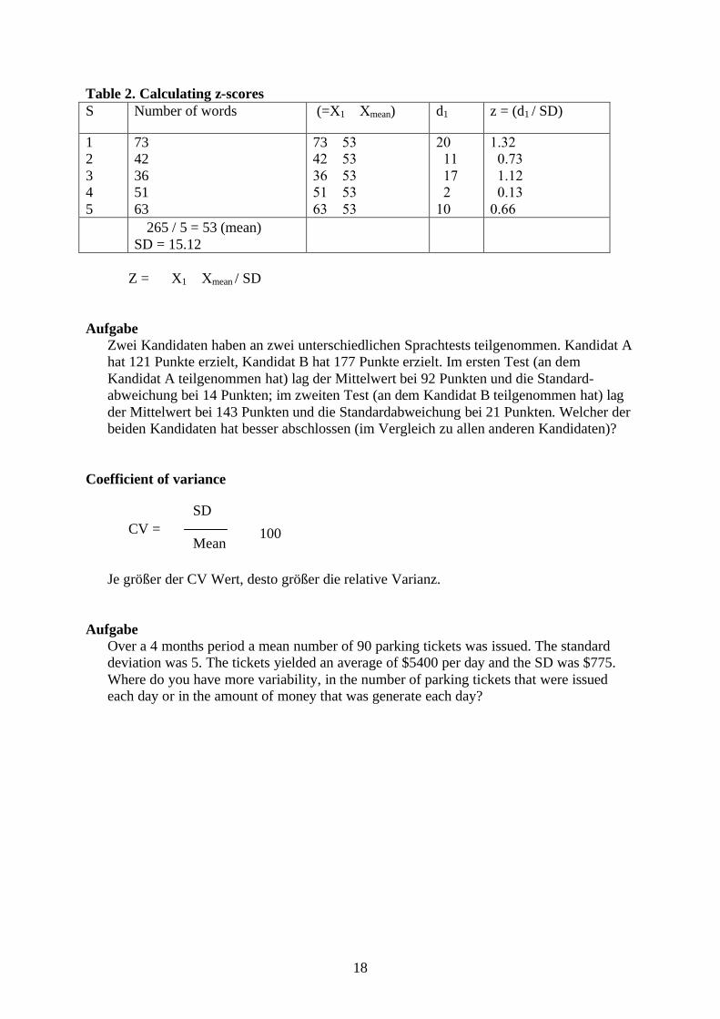
Table 2. Calculating z-scoresS Number of words (=X1 – Xmean) d1 z = (d1 / SD)

12345

7342365163

73 – 53 42 – 5336 – 5351 – 5363 – 53

20–11–17–210

1.32–0.73–1.12–0.130.66

265 / 5 = 53 (mean)SD = 15.12

Z = X1 – Xmean / SD

AufgabeZwei Kandidaten haben an zwei unterschiedlichen Sprachtests teilgenommen. Kandidat A hat 121 Punkte erzielt, Kandidat B hat 177 Punkte erzielt. Im ersten Test (an dem Kandidat A teilgenommen hat) lag der Mittelwert bei 92 Punkten und die Standard-abweichung bei 14 Punkten; im zweiten Test (an dem Kandidat B teilgenommen hat) lag der Mittelwert bei 143 Punkten und die Standardabweichung bei 21 Punkten. Welcher der beiden Kandidaten hat besser abschlossen (im Vergleich zu allen anderen Kandidaten)?

Coefficient of variance

CV =

Je größer der CV Wert, desto größer die relative Varianz.

AufgabeOver a 4 months period a mean number of 90 parking tickets was issued. The standard deviation was 5. The tickets yielded an average of $5400 per day and the SD was $775. Where do you have more variability, in the number of parking tickets that were issued each day or in the amount of money that was generate each day?

SD

Mean 100

19

Introduction to SPSS

Dateneingabe

Die Variablen werden auf dem Blatt ‘Variablenansicht’ eingegeben. Dabei sind bestimmte Konventionen zu beachten. Die Eingaben dürfen

1. nicht länger als 8 Zeichen sein2. nicht mit einer Zahl beginnen (z.B. 1group)3. nicht mit einem Punkt enden4. nicht ein Leerzeichen beinhalten5. nicht die folgenden Zeichen beinhalten: !, ?, *

Correlational analysis

Case Head size Intelligence1 55 1252 59 1323 48 944 60 1105 62 1406 50 96

Experiment (within-subjects)

CASE CONDITION 1 CONDITION 2 CONDITION 31 220 300 2602 250 290 3003 260 280 2904 230 340 1905 190 300 2506 220 270 2407 250 320 2708 280 290 2609 270 340 25010 240 300 350

Experiment (between-subjects)

Case Group Score1 1 32 1 53 1 34 1 25 1 46 1 67 1 98 1 39 1 8… … …

20

Frequency data

DisapproveSex Yes NoFemale 30 20Male 10 40

SEX DISAPPROVE FREQUENCY1 1 30,001 2 20,002 1 10,002 2 40,00

Tables and Figures

bloodgroup

Häufigkeit ProzentGültige

ProzenteKumulierte Prozente

Group A 6 18,8 18,8 18,8Group AB 3 9,4 9,4 28,1

Group B 6 18,8 18,8 46,9Group O 17 53,1 53,1 100,0

Gültig

Gesamt 32 100,0 100,0

sex

Häufigkeit ProzentGültige

ProzenteKumulierte Prozente

Female 16 50,0 50,0 50,0Male 16 50,0 50,0 100,0

Gültig

Gesamt 32 100,0 100,0

21

Group A Group AB Group B Group O

bloodgroup

0

5

10

15

20

Häu

figke

it

bloodgroup

bloodtype * sex Kreuztabelle

Anzahl sex

Female Male GesamtGroup A 3 3 6Group AB 1 2 3Group B 3 3 6

bloodtype

Group O 9 8 17Gesamt 16 16 32

Säulendiagramm

Group A Group AB Group B Group O

bloodgroup

0

2

4

6

8

10

Anz

ahl

sexFemaleMale

22

Histogramm

140 150 160 170 180 190 200

height

0

1

2

3

4

5

6

Häu

figke

it

Mean = 170,28Std. Dev. = 13,679N = 32

Histogramm

Box-and-leaf Plots

Female Malesex

140

150

160

170

180

190

200

heig

ht

3

Streudiagramm Liniendiagramm

140 150 160 170 180 190 200height

40

60

80

100

120

wei

ght

48 50 51 53 55 59 60 62 64 65 67 68 69 70 71 72 75 77 78 80 85 90 95 100

120

weight

140

150

160

170

180

190

200

Mitt

elw

ert h

eigh

t

23

Error Bars Kreisdiagramm

S A P IO OBL GEN

0

1

2

3

4

95%

CI

bloodgroupG r o u p A

G r o u p AB

G r o u p B

G r o u p O

24

Probability and statistical hypothesis testing

Probability

Prior probability

(1) P(6) = 1/6 = 0.166

Probability values range from 0 to 1. Adding all probabilities of the sample yields 1. The probability that an event A will not occur is 1 minus the probability of A. If two events are independent, the probability that one or the other event occurs is the

sum of their individual probabilities. Two events A and B are independent if knowing that the occurrence of A does not

change the probability of the occurrence of B.

Joint probability

(2) a. P(A,B) = P(A) P(B)b. P(5,6) = (0.166) P(0.166) = 0.0277

Conditional probability

(3) P(AB) = P (A B) / P (A)

(4) a. P(NA) = P(A N) / P(N)b. P(NA) = 2.000 / 12.000 = 0.1666

Exercises

(1) In a corpus including 12.000 nouns and 3.500 adjectives, 2.000 adjectives precede a noun. (1) What is the likelihood that a noun occurs after an adjective? (2) What is the likelihood that an adjective precedes a noun?

(2) Determine the probability that a transitive sentence includes a pronominal subject.

0.8 pronominaltransitive

0.2 lexical0.4

0.6 0.6 pronominalintransitive

0.4 lexical

25

Probability distributions

H T

HH HT TH TT

1. 0 girl = HH

2. 1 girl = HT + TH

3. 2 girls = TT

Events Ramdom Variable

Cumulative outcome Probability

012

0.250.500.25

P(x) = 1

ExerciseA coin is tossed three times. Determine the probability of obtaining exactly 2 tails.

HH

HT

TH

TT

0

1

3

26

Binomial distribution

A Bernouli trail has the following properties:

1. two possible outcomes on each trail2. the outcomes are independent of each other3. the probability ratio is constant across trails

The binomial distribution has the following properties: It is based on categorical / nominal data. There are exactly two outcomes for each trail. All trials are independent. The probability of the outcomes is the same for each trail. A sequence of Bernoulli trails gives us the binominal distribution.

Normal distribution

Wenn sie eine Münze 8 Mal werfen, wie hoch ist die Wahrscheinlichkeit, dass sie 8 Mal Kopf bekommen, 7 Mal Kopf, 6 Mal Kopf … ? Die Graphik zeigt, dass die Wahrscheinlichkeit, dass sie 4 Mal Kopf und 4 Mal Zahl bekommen, am größten ist.

27

The normal distribution has the following properties: The center of the curve represents the mean, median, and mode. The curve is symmetrical around the mean. The tails meet the x-axis in infinity. The curve is bell-shaped. The total area under the curve is equal to 1 (by definition).

Other distributions

Empirical rule

28

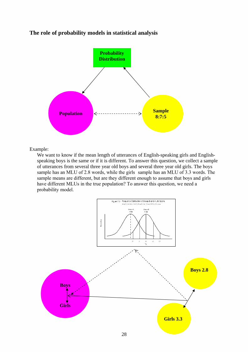
The role of probability models in statistical analysis

Example: We want to know if the mean length of utterances of English-speaking girls and English-speaking boys is the same or if it is different. To answer this question, we collect a sample of utterances from several three year old boys and several three year old girls. The boys’ sample has an MLU of 2.8 words, while the girls’ sample has an MLU of 3.3 words. The sample means are different, but are they different enough to assume that boys and girls have different MLUs in the true population? To answer this question, we need a probability model.

Population Sample8:7:5

Probability Distribution

Boys

Girls

Boys 2.8

Girls 3.3

29

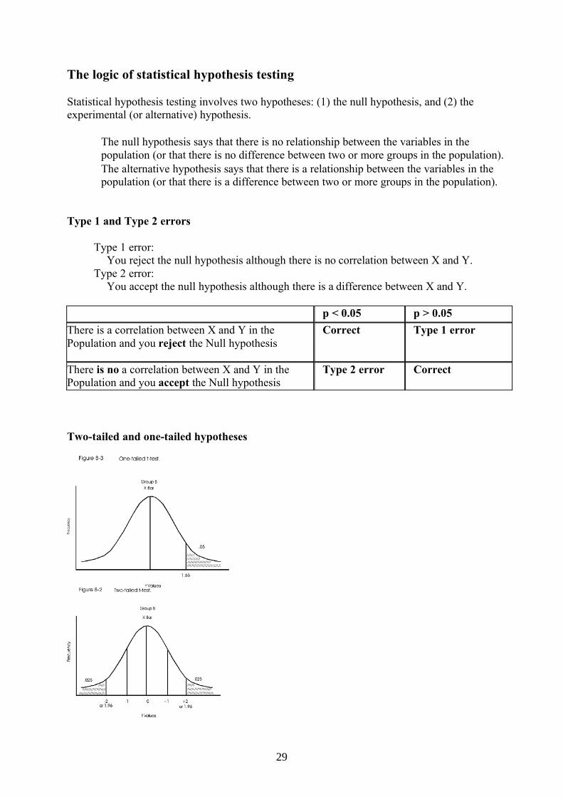
The logic of statistical hypothesis testing

Statistical hypothesis testing involves two hypotheses: (1) the null hypothesis, and (2) the experimental (or alternative) hypothesis.

The null hypothesis says that there is no relationship between the variables in the population (or that there is no difference between two or more groups in the population).

The alternative hypothesis says that there is a relationship between the variables in thepopulation (or that there is a difference between two or more groups in the population).

Type 1 and Type 2 errors

Type 1 error: You reject the null hypothesis although there is no correlation between X and Y.

Type 2 error: You accept the null hypothesis although there is a difference between X and Y.

p < 0.05 p > 0.05There is a correlation between X and Y in thePopulation and you reject the Null hypothesis

Correct Type 1 error

There is no a correlation between X and Y in the Population and you accept the Null hypothesis

Type 2 error Correct

Two-tailed and one-tailed hypotheses

30

Classification of statistical tests

Correlational tests vs. difference test Parametric tests vs. non-parametric tests Between subjects tests vs. within subjects tests Number of conditions Number of independent variables

Power

Factors determining the power level of a test: [the effect size (which is what we are interested in)] [the level of significance that we assume (e.g. p < 0.05)] the sample size: the more subjects the more power the type of test: parametric tests are more powerful than non-parametric test the experimental design: a within-subject design is more powerful than a between-subject

design the direction of the experimental hypothesis: a test involving a one-tailed hypothesis is

more powerful than a test involving a two-tailed hypothesis

Aufgabe1 (p 152)2 (p 153)

31

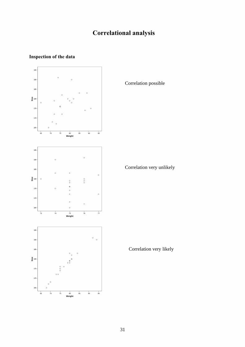
Correlational analysis

Inspection of the data

65 70 75 80 85 90 95

Weight

165

170

175

180

185

190

195

Siz

e

73 74 75 76 77

Weight

165

170

175

180

185

190

195

Siz

e

65 70 75 80 85 90 95

Weight

165

170

175

180

185

190

195

Siz

e

Correlation possible

Correlation very unlikely

Correlation very likely

32

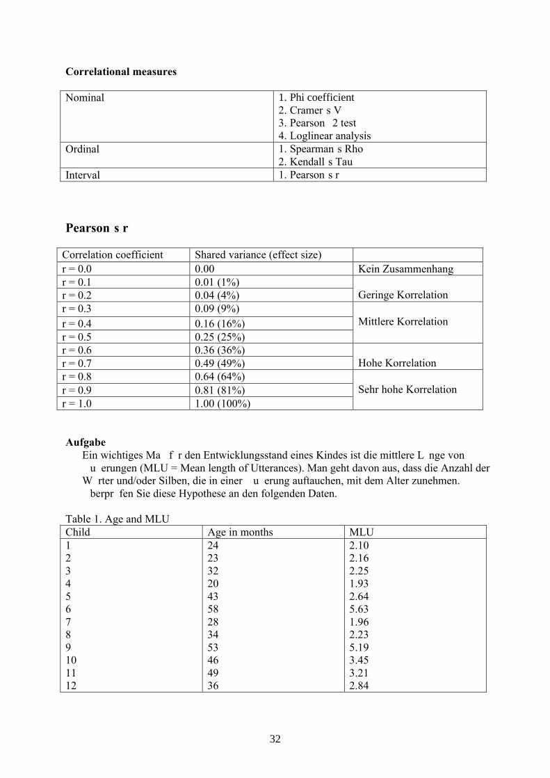
Correlational measures

Nominal 1. Phi coefficient2. Cramer’s V3. Pearson ø2 test4. Loglinear analysis

Ordinal 1. Spearman’s Rho2. Kendall’s Tau

Interval 1. Pearson’s r

Pearson’s r

Correlation coefficient Shared variance (effect size)r = 0.0 0.00 Kein Zusammenhangr = 0.1 0.01 (1%)r = 0.2 0.04 (4%) Geringe Korrelationr = 0.3 0.09 (9%)r = 0.4 0.16 (16%)r = 0.5 0.25 (25%)

Mittlere Korrelation

r = 0.6 0.36 (36%)r = 0.7 0.49 (49%) Hohe Korrelationr = 0.8 0.64 (64%)r = 0.9 0.81 (81%)r = 1.0 1.00 (100%)

Sehr hohe Korrelation

AufgabeEin wichtiges Maß für den Entwicklungsstand eines Kindes ist die mittlere Länge von Äußerungen (MLU = Mean length of Utterances). Man geht davon aus, dass die Anzahl der Wörter und/oder Silben, die in einer Äußerung auftauchen, mit dem Alter zunehmen. Überprüfen Sie diese Hypothese an den folgenden Daten.

Table 1. Age and MLUChild Age in months MLU123456789101112

242332204358283453464936

2.102.162.251.932.645.631.962.235.193.453.212.84

33

Kendell’s Tau and Spearman’s Rho

Beispiel:In einer Studie zur lexikalischen Semantik mussten 15 Probanden eine List von 10 Wörtern danach beurteilen, wie typisch das jeweilige Wort für die Kategorie ‘Fahrzeug’ ist. Dazu mussten sie die Wörter sortieren: 1=sehr typisch, 10=sehr untypisch. Jedes Fahrzeug durfte nur einer Zahl zugewiesen werden. Parallel dazu wurde eine zweite Liste erstellt, in der die Wörter aufgrund ihrer Häufigkeit in einem Korpus geordnet wurden (von 1 bis 10). Frage: Gibt es einen Zusammenhang zwischen der Häufigkeit der Wörter und dem Urteil der Probanden?

Table 1. DataWords Typicality rank Frequency rankcartrucksports carmotor biketrainbicycleshipboatscat boardspace shuttle

12345678910

12653487910

KorrelationenTypicality Frequency

Kendall-Tau-b Typicality Korrelationskoeffizient 1,000 ,733(**)Sig. (2-seitig) . ,003N 10 10

Frequency Korrelationskoeffizient ,733(**) 1,000Sig. (2-seitig) ,003 .N 10 10

Spearman-Rho Typicality Korrelationskoeffizient 1,000 ,879(**)Sig. (2-seitig) . ,001N 10 10

Frequency Korrelationskoeffizient ,879(**) 1,000Sig. (2-seitig) ,001 .N 10 10

** Die Korrelation ist auf dem 0,01 Niveau signifikant (zweiseitig).

34

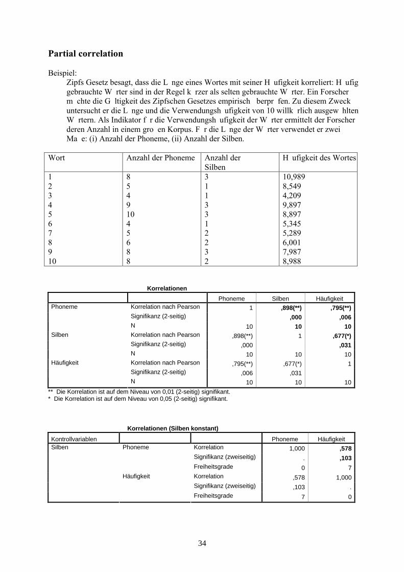
Partial correlation

Beispiel:Zipfs Gesetz besagt, dass die Länge eines Wortes mit seiner Häufigkeit korreliert: Häufig gebrauchte Wörter sind in der Regel kürzer als selten gebrauchte Wörter. Ein Forscher möchte die Gültigkeit des Zipfschen Gesetzes empirisch überprüfen. Zu diesem Zweck untersucht er die Länge und die Verwendungshäufigkeit von 10 willkürlich ausgewählten Wörtern. Als Indikator für die Verwendungshäufigkeit der Wörter ermittelt der Forscher deren Anzahl in einem großen Korpus. Für die Länge der Wörter verwendet er zwei Maße: (i) Anzahl der Phoneme, (ii) Anzahl der Silben.

Wort Anzahl der Phoneme Anzahl derSilben

Häufigkeit des Wortes

12345678910

85491045688

3113312232

10,9898,5494,2099,8978,8975,3455,2896,0017,9878,988

KorrelationenPhoneme Silben Häufigkeit

Korrelation nach Pearson 1 ,898(**) ,795(**)Signifikanz (2-seitig) ,000 ,006

Phoneme

N 10 10 10Korrelation nach Pearson ,898(**) 1 ,677(*)Signifikanz (2-seitig) ,000 ,031

Silben

N 10 10 10Korrelation nach Pearson ,795(**) ,677(*) 1Signifikanz (2-seitig) ,006 ,031

Häufigkeit

N 10 10 10** Die Korrelation ist auf dem Niveau von 0,01 (2-seitig) signifikant.* Die Korrelation ist auf dem Niveau von 0,05 (2-seitig) signifikant.

Korrelationen (Silben konstant)

Kontrollvariablen Phoneme HäufigkeitKorrelation 1,000 ,578Signifikanz (zweiseitig) . ,103

Phoneme

Freiheitsgrade 0 7Korrelation ,578 1,000Signifikanz (zweiseitig) ,103 .

Silben

Häufigkeit

Freiheitsgrade 7 0

35

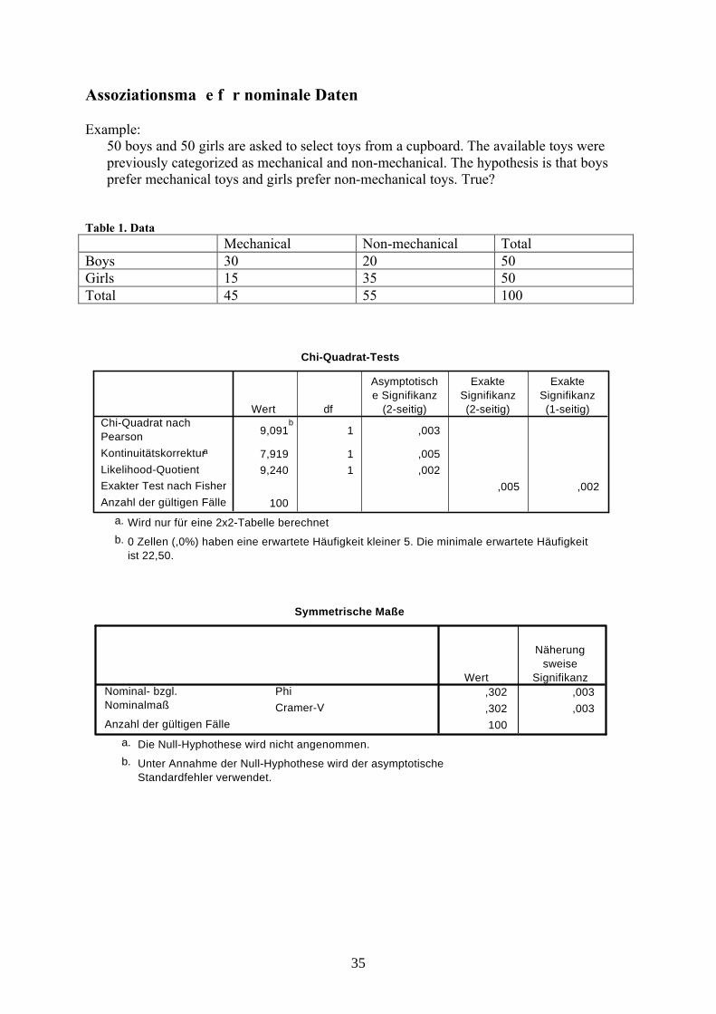
Assoziationsmaße für nominale Daten

Example:50 boys and 50 girls are asked to select toys from a cupboard. The available toys were previously categorized as mechanical and non-mechanical. The hypothesis is that boys prefer mechanical toys and girls prefer non-mechanical toys. True?

Table 1. DataMechanical Non-mechanical Total

Boys 30 20 50Girls 15 35 50Total 45 55 100

Chi-Quadrat-Tests

9,091b

1 ,003

7,919 1 ,0059,240 1 ,002

,005 ,002100

Chi-Quadrat nachPearsonKontinuitätskorrektura

Likelihood-QuotientExakter Test nach FisherAnzahl der gültigen Fälle

Wert df

Asymptotische Signifikanz

(2-seitig)

ExakteSignifikanz(2-seitig)


Wird nur für eine 2x2-Tabelle berechneta.

0 Zellen (,0%) haben eine erwartete Häufigkeit kleiner 5. Die minimale erwartete Häufigkeitist 22,50.

b.

Symmetrische Maße

,302 ,003,302 ,003100

PhiCramer-V

Nominal- bzgl.Nominalmaß

Anzahl der gültigen Fälle

Wert

Näherungsweise

Signifikanz

Die Null-Hyphothese wird nicht angenommen.a.

Unter Annahme der Null-Hyphothese wird der asymptotischeStandardfehler verwendet.

b.

36

Regression

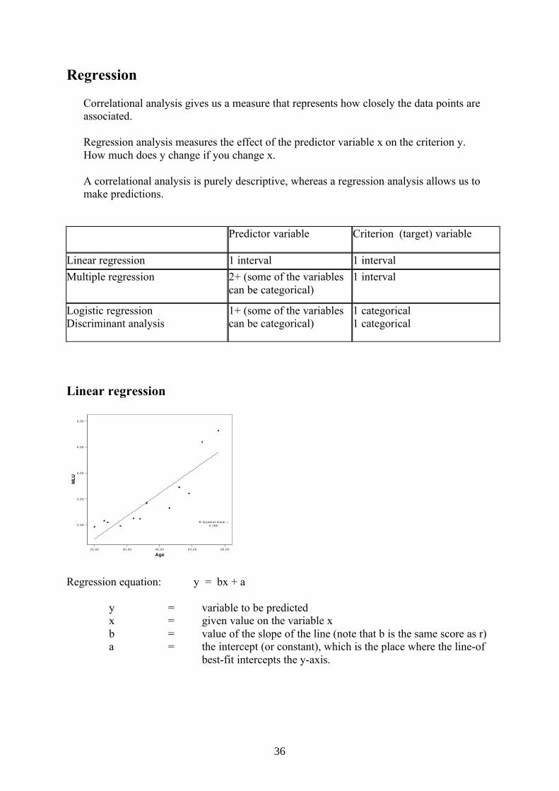
Correlational analysis gives us a measure that represents how closely the data points are associated.

Regression analysis measures the effect of the predictor variable x on the criterion y. –How much does y change if you change x.

A correlational analysis is purely descriptive, whereas a regression analysis allows us to make predictions.

Predictor variable Criterion (target) variable

Linear regression 1 interval 1 intervalMultiple regression 2+ (some of the variables

can be categorical)1 interval

Logistic regressionDiscriminant analysis

1+ (some of the variables can be categorical)

1 categorical1 categorical

Linear regression

20,00 30,00 40,00 50,00 60,00

Age

2,00

3,00

4,00

5,00

6,00

MLU

R-Quadra t l inear = 0,786

Regression equation: y = bx + a

y = variable to be predictedx = given value on the variable xb = value of the slope of the line (note that b is the same score as r)a = the intercept (or constant), which is the place where the line-of

best-fit intercepts the y-axis.

37

ExampleThe table below shows the age of 10 children and their MLU scoure at this age. Use these data to predict how much the MLU score increases relative to the children’s age.

Table 1. Children’s age and MLUChild Age in months MLU123456789101112

242332204358283453464936

2.102.162.251.932.645.631.962.235.193.453.212.84

Modellzusammenfassung

,887a ,786 ,765 ,60242Modell1

R R-QuadratKorrigiertesR-Quadrat

Standardfehler desSchätzers

Einflußvariablen : (Konstante), Agea.

ANOVAb

13,369 1 13,369 36,838 ,000a

3,629 10 ,36316,998 11

RegressionResiduenGesamt

Modell1

Quadratsumme df

Mittel derQuadrate F Signifikanz

Einflußvariablen : (Konstante), Agea.

Abhängige Variable: MLUb.

Koeffizientena

-,304 ,566 -,536 ,603,088 ,014 ,887 6,069 ,000

(Konstante)Age

Modell1

BStandardf

ehler

Nicht standardisierteKoeffizienten

Beta

Standardisierte

Koeffizienten

T Signifikanz

Abhängige Variable: MLUa.

38

Multiple regression

y = b1x1 + b2x2 + b3x3 + … a

1. Simultaneous multiple regression


,875a ,765 ,731 16,913Modell1



Einflußvariablen : (Konstante), Project, Age, IQ,Entrance

a.

ANOVAb

26067,689 4 6516,922 22,783 ,000a

8009,220 28 286,04434076,909 32

RegressionResiduenGesamt

Modell1

Quadratsumme df


Einflußvariablen : (Konstante), Project, Age, IQ, Entrancea.

Abhängige Variable: Finalb.

Koeffizientena

-267,843 48,263 -5,550 ,0002,492 ,459 ,576 5,431 ,0001,057 1,059 ,099 ,998 ,3271,511 ,328 ,447 4,606 ,000

,503 ,355 ,141 1,417 ,168

(Konstante)EntranceAgeIQProject

Modell1

BStandardf

ehler


Beta

Standardisierte

Koeffizienten

T Signifikanz

Abhängige Variable: Finala.

39

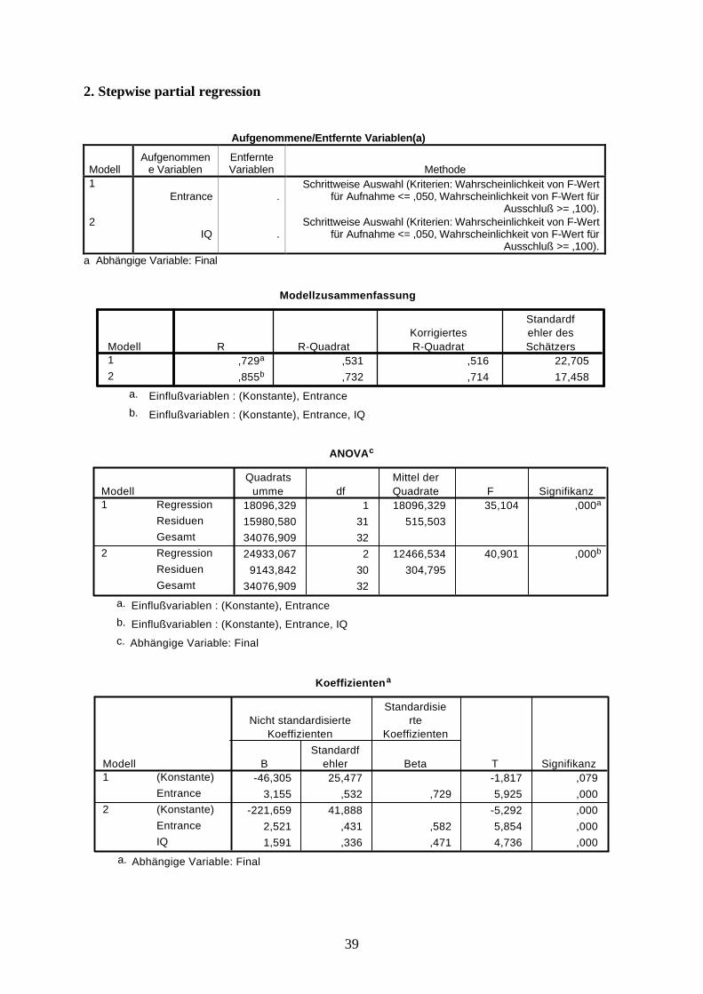
2. Stepwise partial regression

Aufgenommene/Entfernte Variablen(a)

ModellAufgenommen

e VariablenEntfernte Variablen Methode

1Entrance .

Schrittweise Auswahl (Kriterien: Wahrscheinlichkeit von F-Wert für Aufnahme <= ,050, Wahrscheinlichkeit von F-Wert für

Ausschluß >= ,100).2

IQ .Schrittweise Auswahl (Kriterien: Wahrscheinlichkeit von F-Wert

für Aufnahme <= ,050, Wahrscheinlichkeit von F-Wert für Ausschluß >= ,100).

a Abhängige Variable: Final


,729a ,531 ,516 22,705,855b ,732 ,714 17,458

Modell12



Einflußvariablen : (Konstante), Entrancea.

Einflußvariablen : (Konstante), Entrance, IQb.

ANOVAc

18096,329 1 18096,329 35,104 ,000a

15980,580 31 515,50334076,909 3224933,067 2 12466,534 40,901 ,000b

9143,842 30 304,79534076,909 32

RegressionResiduenGesamtRegressionResiduenGesamt

Modell1

2

Quadratsumme df


Einflußvariablen : (Konstante), Entrancea.

Einflußvariablen : (Konstante), Entrance, IQb.

Abhängige Variable: Finalc.

Koeffizientena

-46,305 25,477 -1,817 ,0793,155 ,532 ,729 5,925 ,000

-221,659 41,888 -5,292 ,0002,521 ,431 ,582 5,854 ,0001,591 ,336 ,471 4,736 ,000

(Konstante)Entrance(Konstante)EntranceIQ

Modell1

2

BStandardf

ehler


Beta

Standardisierte

Koeffizienten

T Signifikanz

Abhängige Variable: Finala.

40

One-sample tests

A difference test is often used to find out if there is a difference between two or more groups.

Boys 2.8

Girls 3.3

Boys

Girls

However, sometimes you do not want to know if there is a difference between two samples (or groups), but rather if a sample matches a known distribution.

Sample

The Binomial test

A linguist has collected a sample of sentences including ditransitive verbs from a corpus. Overall, there are 46 sentences in his sample; in 27 sentences the verb occurs with two NP objects, in 19 sentences the verb occurs with an NP and a PP.

(1) a. He gives Peter the ball. V NP NPb. He gives the ball to Peter. V NP PP

41

Test auf Binomialverteilung

Kategorie NBeobachteter

Anteil Testanteil

Asymptotische Signifikanz (2-

seitig)Gruppe 1 27,00 27 ,59 ,50 ,302(a)Gruppe 2 19,00 19 ,41

Frequency

Gesamt 46 1,00a Basiert auf der Z-Approximation.

AufgabeA researcher examined the effectiveness of two new drugs on chronic pain. The first drug was given and pain assessed (Pain1); then a month later the second drug was given and again pain assessed (Pain2). Following the study the researcher wanted to know if the proportions of men and women in the sample used were what would be expected by chance, i.e. 50:50. 15 subjects participated in the study, 10 male and 5 female.

Case Group Pain 1 Pain 2123456789101112131415

111121211221121

252345234123423

232224334243211

Runs test

a. ABABABAABABBABABABABAAABABAb. AAAAAAABAAAAAAABBBBBBBBABBB

Kolmogorov-Smirnov

Used to test if the distribution in your sample is still in the range of what you would expect if the sample is drawn from a normal distribution.

42

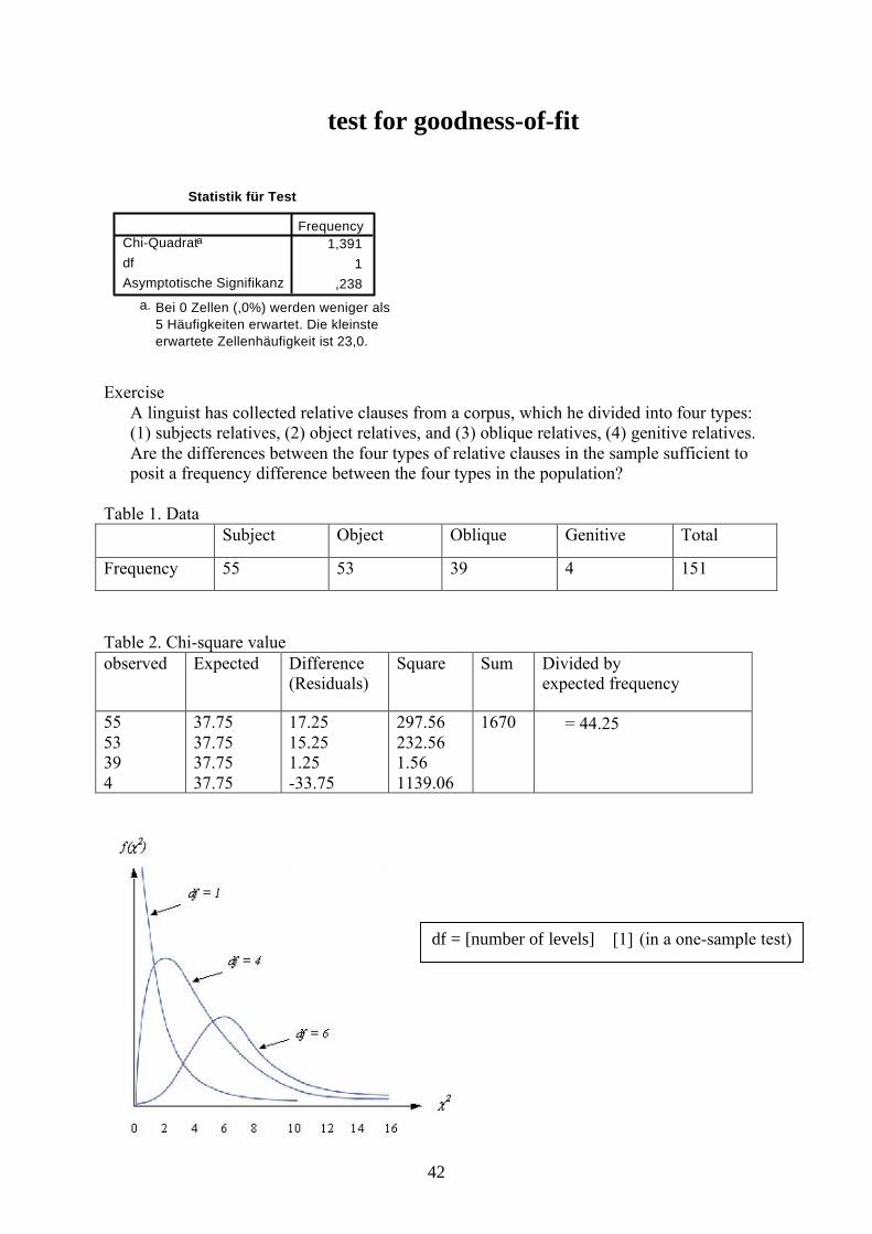
test for goodness-of-fit

Statistik für Test

1,3911

,238

Chi-Quadrata

dfAsymptotische Signifikanz

Frequency

Bei 0 Zellen (,0%) werden weniger als5 Häufigkeiten erwartet. Die kleinsteerwartete Zellenhäufigkeit ist 23,0.

a.

ExerciseA linguist has collected relative clauses from a corpus, which he divided into four types: (1) subjects relatives, (2) object relatives, and (3) oblique relatives, (4) genitive relatives. Are the differences between the four types of relative clauses in the sample sufficient to posit a frequency difference between the four types in the population?

Table 1. DataSubject Object Oblique Genitive Total

Frequency 55 53 39 4 151

Table 2. Chi-square valueobserved Expected Difference

(Residuals)Square Sum Divided by

expected frequency

5553394

37.7537.7537.7537.75

17.2515.251.25-33.75

297.56232.561.561139.06

1670 = 44.25

df = [number of levels] – [1] (in a one-sample test)

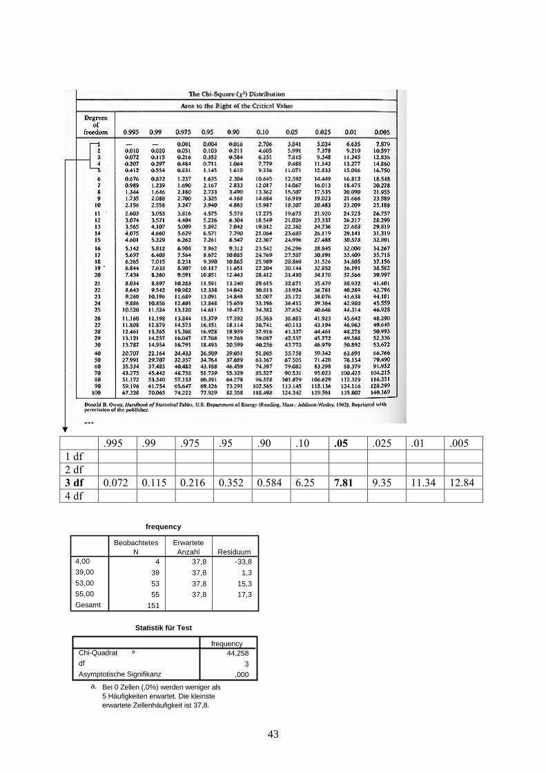
43

.995 .99 .975 .95 .90 .10 .05 .025 .01 .0051 df2 df3 df 0.072 0.115 0.216 0.352 0.584 6.25 7.81 9.35 11.34 12.844 df

frequency

4 37,8 -33,839 37,8 1,353 37,8 15,355 37,8 17,3

151

4,0039,0053,0055,00Gesamt

BeobachtetesN

ErwarteteAnzahl Residuum

Statistik für Test

44,2583

,000

Chi-Quadrat a

dfAsymptotische Signifikanz

frequency

Bei 0 Zellen (,0%) werden weniger als5 Häufigkeiten erwartet. Die kleinsteerwartete Zellenhäufigkeit ist 37,8.

a.

44

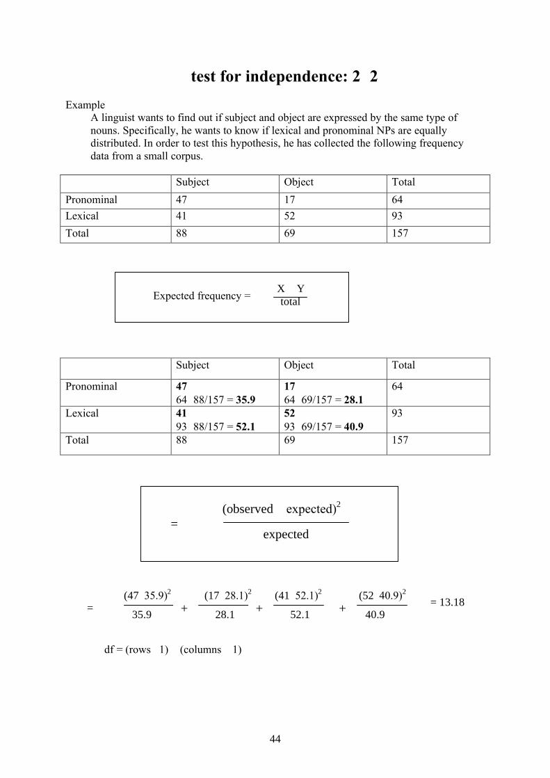
test for independence: 22Example

A linguist wants to find out if subject and object are expressed by the same type of nouns. Specifically, he wants to know if lexical and pronominal NPs are equally distributed. In order to test this hypothesis, he has collected the following frequency data from a small corpus.

Subject Object TotalPronominal 47 17 64Lexical 41 52 93Total 88 69 157

Subject Object Total

Pronominal 476488/157 = 35.9

176469/157 = 28.1

64

Lexical 419388/157 = 52.1

529369/157 = 40.9

93

Total 88 69 157

(47–35.9)2 (17–28.1)2 (41–52.1)2 (52–40.9)2

35.9 28.1 52.1 40.9

df = (rows –1) (columns – 1)

=(observed – expected)2

expected

= = 13.18+ + +

Expected frequency = X Ytotal

45

NPtype * Role KreuztabelleRole

OBJ SUBJ GesamtAnzahl 52 41 93NErwartete Anzahl 40,9 52,1 93,0

Anzahl 17 47 64

NPtype

PROErwartete Anzahl 28,1 35,9 64,0

Anzahl 69 88 157GesamtErwartete Anzahl 69,0 88,0 157,0

Chi-Quadrat-Tests

13,258b

1 ,000

12,094 1 ,00113,628 1 ,000

,000 ,000157

Chi-Quadrat nachPearsonKontinuitätskorrektura

Likelihood-QuotientExakter Test nach FisherAnzahl der gültigen Fälle

Wert df


(2-seitig)



Wird nur für eine 2x2-Tabelle berechneta.

0 Zellen (,0%) haben eine erwartete Häufigkeit kleiner 5. Die minimale erwartete Häufigkeitist 28,13.

b.

Symmetrische Maße

,291 ,000,291 ,000157

PhiCramer-V

Nominal- bzgl.Nominalmaß

Anzahl der gültigen Fälle

Wert

Näherungsweise

Signifikanz

Die Null-Hyphothese wird nicht angenommen.a.

Unter Annahme der Null-Hyphothese wird der asymptotischeStandardfehler verwendet.

b.

Prerequisites of the test of independence:1. each subject provides a score for only one cell2. none of the cells is empty3. not more than 25% of the cells has an expected frequency of less than 5

(which is one cell in a 2 by 2 table)

Fisher exacthttp://www.matforsk.no/ola/fisher.htm

46

McNemar

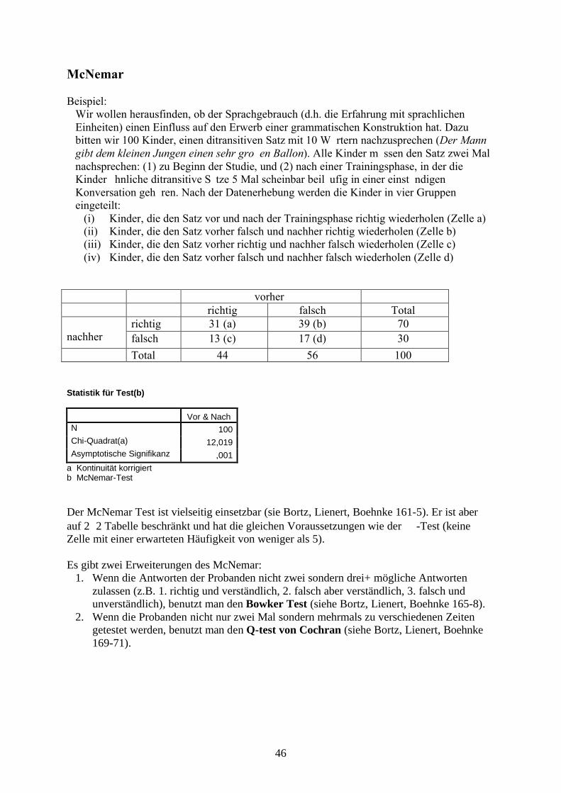
Beispiel:Wir wollen herausfinden, ob der Sprachgebrauch (d.h. die Erfahrung mit sprachlichen Einheiten) einen Einfluss auf den Erwerb einer grammatischen Konstruktion hat. Dazu bitten wir 100 Kinder, einen ditransitiven Satz mit 10 Wörtern nachzusprechen (Der Mann gibt dem kleinen Jungen einen sehr großen Ballon). Alle Kinder müssen den Satz zwei Mal nachsprechen: (1) zu Beginn der Studie, und (2) nach einer Trainingsphase, in der die Kinder ähnliche ditransitive Sätze 5 Mal scheinbar beiläufig in einer einstündigen Konversation gehören. Nach der Datenerhebung werden die Kinder in vier Gruppen eingeteilt:

(i) Kinder, die den Satz vor und nach der Trainingsphase richtig wiederholen (Zelle a)(ii) Kinder, die den Satz vorher falsch und nachher richtig wiederholen (Zelle b)(iii) Kinder, die den Satz vorher richtig und nachher falsch wiederholen (Zelle c)(iv) Kinder, die den Satz vorher falsch und nachher falsch wiederholen (Zelle d)

vorherrichtig falsch Total

richtig 31 (a) 39 (b) 70nachher falsch 13 (c) 17 (d) 30

Total 44 56 100

Statistik für Test(b)

Vor & NachN 100Chi-Quadrat(a) 12,019Asymptotische Signifikanz ,001

a Kontinuität korrigiertb McNemar-Test

Der McNemar Test ist vielseitig einsetzbar (sie Bortz, Lienert, Boehnke 161-5). Er ist aber auf 22 Tabelle beschränkt und hat die gleichen Voraussetzungen wie der -Test (keine Zelle mit einer erwarteten Häufigkeit von weniger als 5).

Es gibt zwei Erweiterungen des McNemar:1. Wenn die Antworten der Probanden nicht zwei sondern drei+ mögliche Antworten

zulassen (z.B. 1. richtig und verständlich, 2. falsch aber verständlich, 3. falsch und unverständlich), benutzt man den Bowker Test (siehe Bortz, Lienert, Boehnke 165-8).

2. Wenn die Probanden nicht nur zwei Mal sondern mehrmals zu verschiedenen Zeiten getestet werden, benutzt man den Q-test von Cochran (siehe Bortz, Lienert, Boehnke 169-71).

47

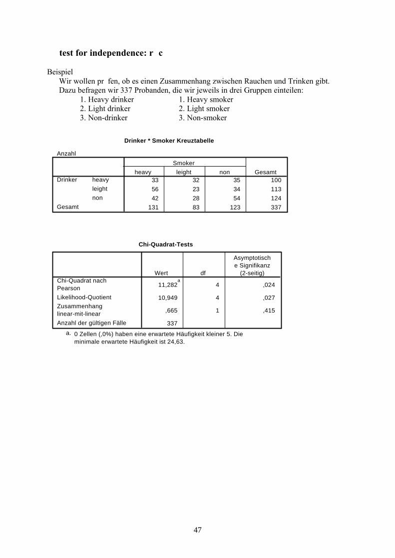
test for independence: rc

BeispielWir wollen prüfen, ob es einen Zusammenhang zwischen Rauchen und Trinken gibt. Dazu befragen wir 337 Probanden, die wir jeweils in drei Gruppen einteilen:

1. Heavy drinker 1. Heavy smoker2. Light drinker 2. Light smoker3. Non-drinker 3. Non-smoker

Drinker * Smoker Kreuztabelle

Anzahl

33 32 35 10056 23 34 11342 28 54 124

131 83 123 337

heavyleightnon

Drinker

Gesamt

heavy leight nonSmoker

Gesamt

Chi-Quadrat-Tests

11,282a

4 ,024

10,949 4 ,027

,665 1 ,415

337

Chi-Quadrat nachPearsonLikelihood-QuotientZusammenhanglinear-mit-linearAnzahl der gültigen Fälle

Wert df


(2-seitig)

0 Zellen (,0%) haben eine erwartete Häufigkeit kleiner 5. Dieminimale erwartete Häufigkeit ist 24,63.

a.

48

Nominaldaten mit zwei oder mehr unabhängigen Variablen

Declarative clauses QuestionsTransitive Intransitive Transitive Transitive Total

Written 23 45 56 12 136Spoken 34 56 32 22 144Total 57 101 88 34 280

Drei Variablen: 1. spoken – written2. declarative – interrogative 3. transitive – intansitive

Um Nominaldaten mit zwei oder mehr unabhängigen Variablen bearbeiten zu können werden besondere statistische Verfahren verwendet:

1. Konfigurationsfrequenzanalyse (KFA)2. Log-lineare Analyse

Konfigurationsfrequenzanalyse (KFC)

BeispielIm Englischen gibt es die Möglichkeit, Relationen zwischen Possessor und Possessed mit zwei Konstruktionen auszudrücken:

1. of-Genitive The cover of the book2. s-Genitive The book’s cover

Die Wahl der Konstruktionen wird durch verschiedene Faktoren bestimmt. Ganz wichtig ist die Semantik der beiden beteiligten NPs. Gries (2002) unterscheidet drei Typen:

1. Abstrakte NPs2. Konkrete NPs3. Menschliche NPs

Daraus ergibt sich folgende Variablenausprägung:

Possessed Abstract Concrete Human TotalPossessor of s of s of s of s TotalAbstract 80 37 9 8 3 2 92 47 139Concrete 22 0 20 1 0 0 42 1 43Human 9 58 1 35 6 9 16 102 118

111 95 30 44 9 11Total206 74 20

150 150 300

Eine KFC prüft, ob die Häufigkeiten bestimmter Konfigurationen höher oder niedriger sind als man vom Zufall her erwarten würde. Ist eine Konfiguration signifikant häufiger, wird sie als Typ bezeichnet; ist eine Konfiguration signifikant seltener, wird sie als Antitypbezeichnet. Die folgende Tabelle zeigt, dass die KFA auf einem Chi-Quadrat Test basiert.

49

Possessor Possessed Type Observed Expected Residuals

Abstract Abstract of 80 130206150 3002

(80 – 47.72)2

47.72

Abstract Abstract s 37 47.72 2,41Abstract Concrete of 9 17.14 3.87Abstract Concrete s 8 17.14 4.88Abstract Human of 3 4.63 0.58Abstract Human s 2 4.63 1.5Concrete Concrete s 22 14.76 3.55Concrete Concrete of 0 14.76 14.76Concrete Abstract s 20 5.3 40.73Concrete Abstract of 1 5.3 3.49Concrete Human s 0 1.43 1.43Concrete Human s 0 1.43 1.43Human Abstract s 9 40.51 24.51Human Abstract of 58 40.51 7.55Human Concrete s 1 14.55 12.62Human Concrete of 35 14.55 28.73Human Human s 5 3.93 1.09Human Human s 9 3.93 6.53

Summen 300 300 181,54 ()

In der Spalte expected Frequency sind die erwarteten Häufigkeiten ausgerechnet worden, indem man wie beim -test alle Randhäufigkeiten einer Konfiguration multipliziert und durch N dividiert. Die -Werte, die über einem bestimmten Signifikanzniveaus liegen, sind signifikante Typen bzw. Antitypen:

Typen1. [abstract possessor] [abstract possessed] of2. [concrete possessor] [concrete possessed] of3. [human possessor] [concrete possessed] sAntitypen1. [concrete possessor] [abstrcat possessed] s2. [human possessor] [concrete possessed] of3. [humn possessor] [abstract possessed] of

Anders als beim einfachen -Test sind die -Komponenten der einzelnen Felder bei der KFA nicht voneinander unabhängig. Die KFA ist deshalb in erster Linie ein heuristisches Verfahren, das dazu dient besonders auffällige Typen und Antitypen aufzuspüren, die dann anhand von neuen Daten nochmals überprüft werden müssen (siehe Bortz, Lienert, Boehnke 155-157).

= 21.83= 47.72

50

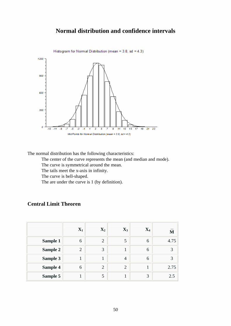
Normal distribution and confidence intervals

The normal distribution has the following characteristics: The center of the curve represents the mean (and median and mode). The curve is symmetrical around the mean. The tails meet the x-axis in infinity. The curve is bell-shaped. The are under the curve is 1 (by definition).

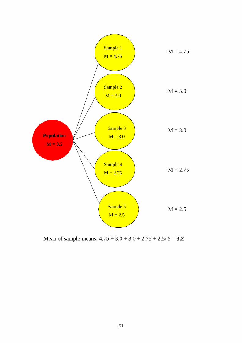
Central Limit Theoren

X1 X2 X3 X4 M

Sample 1 6 2 5 6 4.75

Sample 2 2 3 1 6 3

Sample 3 1 1 4 6 3

Sample 4 6 2 2 1 2.75

Sample 5 1 5 1 3 2.5

51

M = 4.75

M = 3.0

M = 3.0

M = 2.75

M = 2.5

Mean of sample means: 4.75 + 3.0 + 3.0 + 2.75 + 2.5/ 5 = 3.2

Population

M = 3.5

Sample 1

M = 4.75

Sample 2

M = 3.0

Sample 3

M = 3.0

Sample 4

M = 2.75

Sample 5

M = 2.5

52

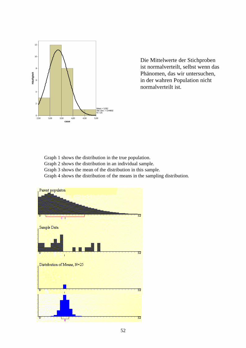
Graph 1 shows the distribution in the true population. Graph 2 shows the distribution in an individual sample. Graph 3 shows the mean of the distribution in this sample. Graph 4 shows the distribution of the means in the sampling distribution.

2,50 3,00 3,50 4,00 4,50 5,00case

0

2

4

6

8

10

12

Häu

figke

it

Mean = 3,352Std. Dev. = 0,44802N = 25

Die Mittelwerte der Stichproben ist normalverteilt, selbst wenn das Phänomen, das wir untersuchen, in der wahren Population nicht normalverteilt ist.

53

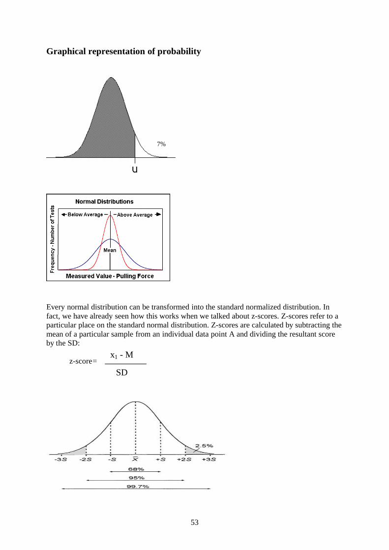
Graphical representation of probability

Every normal distribution can be transformed into the standard normalized distribution. In fact, we have already seen how this works when we talked about z-scores. Z-scores refer to a particular place on the standard normal distribution. Z-scores are calculated by subtracting the mean of a particular sample from an individual data point A and dividing the resultant score by the SD:

z-score=

7%

x1 - M

SD

54

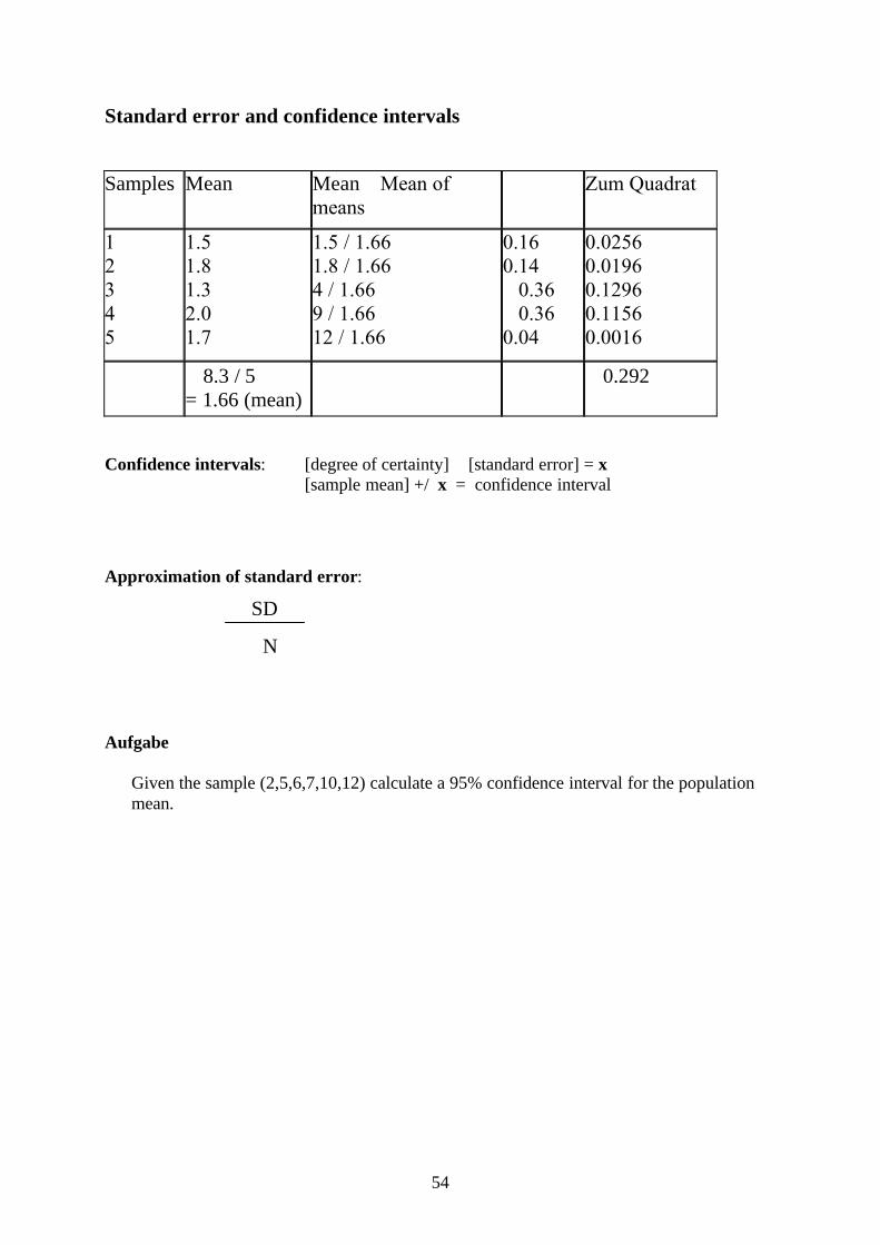
Standard error and confidence intervals

Samples Mean Mean – Mean of means

Zum Quadrat

12345

1.51.81.32.01.7

1.5 / 1.661.8 / 1.664 / 1.669 / 1.6612 / 1.66

0.160.14– 0.36– 0.360.04

0.02560.01960.12960.11560.0016

8.3 / 5= 1.66 (mean)

0.292

Confidence intervals: [degree of certainty] [standard error] = x[sample mean] +/–x = confidence interval

Approximation of standard error:

SD

N

Aufgabe

Given the sample (2,5,6,7,10,12) calculate a 95% confidence interval for the population mean.

55

T-test, U-test, Wilcoxon

Overview of tests

Parametric Non-parametricbetween / independent / unrelated

Independent t-test Mann-Whitney U

within / dependent / related / repeated measures

Paired t-test Wilcoxon

Independent t-test

Example (from the textbook): 24 people were involved in an experiment to determine whether background noise (e.g. music) affects short-term memory (recall of words). Half of the sample was randomly allocated to the NOISE condition, and half to the NO NOISE condition. The participants in the NOISE condition tried to memorize a list of 20 words in two minutes, while listening to pre-recorded noise through earphones. The other participants wore earphones but heard no noise as they attempted to memorize the words. Immediately after this, they were tested to see how many words they recalled. Table 1 shows the raw results.

Mean1 = 2.34

Mean2 = 2.01

One category or two?

Does the difference between mean 1 and mean 2 reflect a difference in the population?

56

Table 1. Data for a t-testNOISE (group 1) NO NOISE (group 2)5.0010.006.006.007.003.006.009.005.0010.0011.009.00

15.009.0016.0015.0016.0018.0017.0013.0011.0012.0013.0011.00

=87X=7.3SD=2.5

=166X=13.8SD=2.8

1,00 2,00

Group

3,00

6,00

9,00

12,00

15,00

18,00

Sco

re

Within group variance (SD)

Between group variance (difference) between M1 and M2

57

Effect size of t-test

M1 – M2: 7.3 – 13.8 = –6.5

Mean SD: SD 1 – SD 2 / 2 = 2.5 2.8 / 2 = 2.65

M1 – M2

Mean SD

6.5

2.65

Table 1. Effect size of t-testEffect size d Percentage of overlapSmallMediumLarge

0.20.50.8

856753

Prerequisites of the t-test1. For small samples (i.e. N < 15), the data must be normally distributed.2. The data must be continuous (though the t-test is also often used for ordinal data.3. Homogeneity-of-variance (Levene’s test)

d =

= 2.45= d =

58

ExampleThe word that is ambiguous. Among other things, it can be a demonstrative (e.g. That’s my car) and a complementizer (e.g. I regret that I didn’t go). The two categories tend to occur in different contexts. At the beginning of a sentence, that tends to be a demonstrative and is only rarely a complementizer, but after verbs that is usually a complementizer and only rarely a demonstrative. A psycholinguist wants to know if the different frequencies of the demonstrative and complementizer affect the interpretation of that in different contexts. In order to test this hypothesis, he measures the reading times (i.e. the time it takes to move from one word to another while reading a sentence) of the complementizer and the demonstrative after verbs that frequently occur with sentential complements but may also occur with an NP including a demonstrative (e.g. find, know, regret). Since the complementizer is more frequent in this context than the demonstrative, it is reasonable to assume that the complementizer has shorter reading times than the demonstrative. Twenty subjects were tested: 10 subjects listened to sentences in which the verbs were followed by a that-clause, and 10 subjects listened to sentences that were followed by an NP including a that-determiner. Table 1 shows the reading times.

(1) Peter know that she was coming.(2) Peter know that guy.

Group 1 That-clauses Group 2 That-NPs12345678910

500513300561483502539467420480

11121314151617181920

392445271523421489501388411467

Test bei unabhängigen Stichproben

Levene-Test T-Test für die Mittelwertgleichheit

F Sig T dfSig. (2-seitig)

Mittlere Differenz

Standardfehler der Differenz

95% Konfidenzintervall der

Differenz

Untere ObereScore Varianzen

sind gleich ,068 ,797 1,401 18 ,178 45,70000 32,61903 -22,83004 114,23004

Varianzen sind nicht gleich

1,401 18,00 ,178 45,70000 32,61903 -22,83012 114,23012

59

Test bei unabhängigen Stichproben

Levene-Test T-Test für die Mittelwertgleichheit

F Sig T df

Sig. (2-

seitig)Mittlere

Differenz

Standard-fehler der Differenz

95% Konfidenzintervall der

Differenz

Untere ObereScore Varianzen

sindgleich

,997 ,333 2,229 16 ,040 47,55556 21,33500 2,32738 92,78373

Varianzen sind nicht gleich

2,229 15,504 ,041 47,55556 21,33500 2,20960 92,90151

Paired t-test

ExerciseAnalyze the same data using a paired t-Test.

Statistik bei gepaarten Stichproben

476,5000 10 73,08329 23,11096430,8000 10 72,79316 23,01922

Condition1Condition2

Paaren1

Mittelwert NStandardabweichung

Standardfehler des

Mittelwertes

Korrelationen bei gepaarten Stichproben

10 ,899 ,000Condition1 & Condition2Paaren 1N Korrelation Signifikanz

Test bei gepaarten Stichproben

Gepaarte Differenzen T dfSig.

(2-seitig)

MittelwertStandard-

abweichung

Standardfehler des

Mittelwertes

95% Konfidenzintervall

der Differenz

Untere OberePaaren 1

Condition1 Condition2 45,70000 32,72121 10,34736 22,292

65 69,10735 4,417 9 ,002

60

Non-parametric equivalents of the t-test

Non-parametric equivalents of the t-tests must be used:1. when we have ordinal data2. when we have interval data, but the samples are very small3. when we have interval data, but the distribution is skewed (i.e. not normal)4. when we have interval data, but unequal sample sizes.

Mann-Whitney

Example:When children begin to speak, there is often great variation in the pronunciation of particular speech sounds. A researcher wants to find out if a two-year old child pronounces /g/ and /k/ differently or if the two speech sounds are basically pronounced in the same way at this age. In adult language, /g/ and /k/ are primarily distinguished by voice onset time, i.e.VOT. In order to decide if two-year old children pronounce /g/ and /k/ differently, the researcher collects a (very small) corpus of 13 words, six words including /g/ in adult language and seven words including /k/ in adult language. The words were selected such that /g/ and /k/ are surrounded by the same speech sounds (i.e. they occur in the same phonetic environment). For each word, the researcher measured the voice onset time in milliseconds. Are the two speech sounds significantly different in the child’s speech?

Table 1. Data for Mann-WhitneySpeech sound VOT in msc Ranks/g//g//g//g//g//g//k//k//k//k//k//k//k/

381955635189125731383551190169

313614.58971024.51211

61

1,00 2,00

group

0,00

50,00

100,00

150,00

200,00m

sc2

Ränge

6 5,92 35,507 7,93 55,50

13

group1,002,00Gesamt

mscN Mittlerer Rang Rangsumme


mscMann-Whitney-U 14,500Wilcoxon-W 35,500Z -,930Asymptotische Signifikanz (2-seitig)

,352

Exakte Signifikanz [2*(1-seitig Sig.)],366(a)

a Nicht für Bindungen korrigiert.b Gruppenvariable: group

Wilcoxon

Example:Nurses were asked to rate their sympathy on a scale between 1 and 10 for MS patients before and after talking to them. Table 1 shows the nurses’ sympathy scores before and after they have talked to them. Have the scores changed?

62

Table 1. Data for the WilcoxonBefore After

5.006.002.004.006.007.003.005.005.005.00

7.006.003.008.007.006.007.008.005.008.00

Mean: 4.8SD: 1.48Median: 5

Mean: 6.5SD: 1.58Median: 7

Table 2. Intermediate results of the WilcoxonDifference between scores from individual

subjectsRanking of the scores in the left-hand

column–20

–1–4–1+1–4–30

–3

4–2

7.522

7.55.5–

5.57 minuses, 1 plus

2,00 3,00 4,00 5,00 6,00 7,00

Before

0

1

2

3

4

Häu

figke

it

Mean = 4,80Std. Dev. = 1,47573N = 10

3,00 4,00 5,00 6,00 7,00 8,00

After

0,0

0,5

1,0

1,5

2,0

2,5

3,0

Häu

figke

it

Mean = 6,50Std. Dev. = 1,58114N = 10

63

Ränge

1a 2,00 2,007b 4,86 34,002c

10

Negative RängePositive RängeBindungenGesamt

After - BeforeN Mittlerer Rang Rangsumme

After < Beforea.

After > Beforeb.

After = Beforec.

Statistik für Test b

-2,257a

,024

ZAsymptotischeSignifikanz (2-seitig)

After - Before

Basiert auf negativen Rängen.a.

Wilcoxon-Testb.

Experimental design

The t-test is a parametric test that should only be used for interval data. Many psycholinguistic experiments involve interval data: reaction time studies, eye-tracking studies, etc. Interval data provides more information than ordinal data or simple frequency counts and it can be analyzed by means of the most powerful tests. Therefore psychologists always try to work with interval data. But of course, not all experimental tasks generate interval data. There are tasks in which subjects are asked to make a choice between alternatives (forced choice tasks) and there are tasks in which the experimenter divides the subjects’ responses into discrete categories (e.g. correct vs. incorrect).

In such a case, we have to use statistical tests for the analysis of frequency data or ordinal data; but that should always be the last resort. If possible we would like to base our analysis on normally distributed interval data. So what can we do?

We can design the experiment in such a way that frequency or ordinal data approximates interval data. There are several things we can do:

1. We can try to find a reasonable coding scheme that distinguishes more than two categories.

2. We can test subjects multiple times on the same condition.

For instance, in a study on the acquisition of relative clauses, we wanted to know if subject and object relative clause cause different problems for pre-school children. So we designed an experiment in which each child had to repeat subject and object relative clauses. We then assigned one of three possible scores to each response:

1.0 score for correct repetition0.5 for partially correct repetitions0.0 for incorrect repetitions

64

Each child was given 4 subject relative clauses and 4 object relative clauses (presented in random order and separated by filler sentences). Thus, four each of the two categories (SUBJ and OBJ) a child could obtain a score between zero and four on a scale with 9 possible outcomes:

0.0 – 0.5 – 1.0 – 1.5 – 2.0 – 2.5 – 3.0 – 3.5 – 4.0

This procedure yields a scale that approximates interval data and allows you to calculate amean score for each child. For instance, assume a child obtained the following 4 scores:

1 – 0 – 0.5 – 1 = 2.5/4 = 0.625 (mean score on each trail)

In this way, you get a mean score for each category for each child. Moreover, if you look at the data, you find that they are approximately normally distributed.

Exercise:First, determine if the A and P relative clauses are normally distributed in the Diessel&Tomasello (2005) study. Second, determine if the children of this study performed differently on A and P relative clauses.

65

One-sample t-test

Example:Previous research has shown that English-speaking children have an MLU of 3.0 at age 3;2. A researcher wants to know if SLI children (i.e. children with a specific language impairment) have a lower (or higher MLU) at this age. We know that SLI children have difficulties in processing morphological units, but it is unclear if their MLUs are lower than in normally developing children. In order to test this hypothesis, the researcher collected data from 24 SLI children aged 3;1 to 3;3 and determined the MLU for each child.

Table 1. MLU of 24 SLI children aged 3;1-3;3Child MLU123456789101112131415161718192021222324

2,73,02,82,93,13,03,12,53,23,12,92,92,83,13,22,42,32,83,12,52,72,92,93,0

66

Univariate Statistiken (confidence intervals)

StatistikStandardfe

hlerMittelwert 2,8708 ,05089

Untergrenze 2,765695% Konfidenzintervall des Mittelwerts

Obergrenze2,9761

5% getrimmtes Mittel 2,8833Median 2,9000Varianz ,062Standardabweichung ,24931Minimum 2,30Maximum 3,20Spannweite ,90Interquartilbereich ,38Schiefe -,812 ,472

Score

Kurtosis -,029 ,918

Statistik bei einer Stichprobe

N MittelwertStandardabweich

ungStandardfehler

des MittelwertesScore 24 2,8708 ,24931 ,05089

Test bei einer Sichprobe

-4,503 23 ,000 -,22917 -,3344 -,1239ScoreT df Sig. (2-seitig)

MittlereDifferenz Untere Obere

95% Konfidenzintervallder Differenz

Testwert = 3.1

67

ANOVA

Table 1. Overview of one-way testsParametric Non-parametric

Between subjects Independent ANOVA Kruskal Wallis

Within subjects Repeated measures ANOVA Friedman’s ANOVA

Independent one-way ANOVA

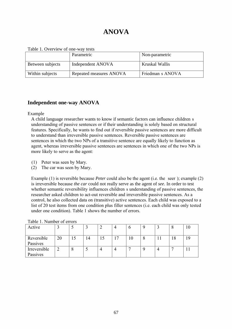
ExampleA child language researcher wants to know if semantic factors can influence children’s understanding of passive sentences or if their understanding is solely based on structural features. Specifically, he wants to find out if reversible passive sentences are more difficult to understand than irreversible passive sentences. Reversible passive sentences are sentences in which the two NPs of a transitive sentence are equally likely to function as agent, whereas irreversible passive sentences are sentences in which one of the two NPs is more likely to serve as the agent:

(1) Peter was seen by Mary.(2) The car was seen by Mary.

Example (1) is reversible because Peter could also be the agent (i.e. the ‘seer’); example (2) is irreversible because the car could not really serve as the agent of see. In order to test whether semantic reversibility influences children’s understanding of passive sentences, the researcher asked children to act-out reversible and irreversible passive sentences. As a control, he also collected data on (transitive) active sentences. Each child was exposed to a list of 20 test items from one condition plus filler sentences (i.e. each child was only tested under one condition). Table 1 shows the number of errors.

Table 1. Number of errorsActive 3 5 3 2 4 6 9 3 8 10

ReversiblePassives

20 15 14 15 17 10 8 11 18 19

IrreversiblePassives

2 8 5 4 4 7 9 4 7 11

68

1,00 2,00 3,00

Group

0,00

5,00

10,00

15,00

20,00

Scor

es

The ANOVA is based on the following measures:1. mean of each group2. the grand mean, i.e. the mean of the three means3. the variation within each group4. the deviation of each group mean from the grand mean 5. the total variance, which is the combined variability of within-group variation and

between-group variation.

The ANOVA calculates a test statistics, i.e. the F-value, which represents something like the average of (1) the within groups variance, (2) the between groups variance, and (3) the total variance of the three group.

You can also think of the F-value as the ratio of the between-groups variance and the within-groups variance:

Between-groups variance

Within groups varianceF ratio =

69

Post hoc tests

(i) Planned comparisons:1. active – reversible passive2. active – irreversible passive3. reversible passive – irreversible passive

1 test: .05 / 1 = .0502 tests .05 / 2 = .0253 tests .05 / 3 = .016

(ii) Post hoc tests(1) Tukey Honstly Significance Difference (HSD)(2) Least Significant Difference (LSD)

ONEWAY deskriptive Statistiken

N MittelwertStandardabweichung

Standardfehler

95%-Konfidenzintervall für den Mittelwert Minimum Maximum

Untergrenze

Obergrenze

1,00 10 5,3000 2,83039 ,89505 3,2753 7,3247 2,00 10,002,00 10 14,7000 4,00139 1,26535 11,8376 17,5624 8,00 20,003,00 10 6,1000 2,76687 ,87496 4,1207 8,0793 2,00 11,00Total 30 8,7000 5,34435 ,97574 6,7044 10,6956 2,00 20,00

ONEWAY ANOVA

Scores

543,200 2 271,600 25,722 ,000285,100 27 10,559828,300 29

Zwischen den GruppenInnerhalb der GruppenGesamt

Quadratsumme df


Mehrfachvergleiche

Abhängige Variable: Scores

-9,40000* 1,45322 ,000 -13,0031 -5,7969-,80000 1,45322 ,847 -4,4031 2,80319,40000* 1,45322 ,000 5,7969 13,00318,60000* 1,45322 ,000 4,9969 12,2031

,80000 1,45322 ,847 -2,8031 4,4031-8,60000* 1,45322 ,000 -12,2031 -4,9969-9,40000* 1,45322 ,000 -12,3818 -6,4182

-,80000 1,45322 ,587 -3,7818 2,18189,40000* 1,45322 ,000 6,4182 12,38188,60000* 1,45322 ,000 5,6182 11,5818

,80000 1,45322 ,587 -2,1818 3,7818-8,60000* 1,45322 ,000 -11,5818 -5,6182

(J) Group2,003,001,003,001,002,002,003,001,003,001,002,00

(I) Group1,00

2,00

3,00

1,00

2,00

3,00

Tukey-HSD

LSD

MittlereDifferenz (I-J)

Standardfehler Signifikanz Untergrenze Obergrenze

95%-Konfidenzintervall

Die mittlere Differenz ist auf der Stufe .05 signifikant.*.

Zusammenhangsmaße

,810 ,656Scores * GroupEta Eta-Quadrat

70

Kruskal-Wallis

BeispielEin Linguist möchte wissen, ob sich die Länge von vorangestellten Adverbialsätzen mit dem Diskurstyp verändert. Drei Diskurstypen werden untersucht: (1) informeller mündlicher Diskurs, (2) akademischer mündlicher Diskurs, (3) Verkaufsgespräch. Um diese Frage zu beantworten, wertet der Linguist Transkriptionen von 15 Personen aus: 4 akademische Diskurse, 7 informelle Diskurse, und 4 Verkaufsgespräche.

Gesprächstype Durchschnittliche Länge des ADV-SatzesAkademischAkademischAkademischAkademischInformellInformellInformellInformellInformellInformellInformellVerkaufsgesprächVerkaufsgesprächVerkaufsgesprächVerkaufsgespräch

131511124462534910105

Ränge

Group N Mittlerer RangLength 1,00 4 13,50

2,00 7 4,213,00 4 9,13Gesamt 15

Statistik für Test a,b

11,4422

,003

Chi-QuadratdfAsymptotische Signifikanz

Length

Kruskal-Wallis-Testa.

Gruppenvariable: Groupb.

71

Statistik für Testb

,00028,000-2,670

,008

,006a

Mann-Whitney-UWilcoxon-WZAsymptotischeSignifikanz (2-seitig)Exakte Signifikanz[2*(1-seitig Sig.)]

Length

Nicht für Bindungen korrigiert.a.



LengthMann-Whitney-U ,000Wilcoxon-W 10,000Z -2,323Asymptotische Signifikanz (2-seitig) ,020

Exakte Signifikanz [2*(1-seitig Sig.)] ,029(a)

a Nicht für Bindungen korrigiert.b Gruppenvariable: Group


1,50029,500-2,395

,017

,012a

Mann-Whitney-UWilcoxon-WZAsymptotischeSignifikanz (2-seitig)Exakte Signifikanz[2*(1-seitig Sig.)]

Length

Nicht für Bindungen korrigiert.a.


1. Akademisch – Informell z=2.67; p<0.006

2. Akademisch – Verkaufsgespräch z=2.32; p<0.020

3. Informell – Verkaufsgespräch z=2.40; p<0.012

Akademisch vs. Informell

Akademisch vs. Verkaufsgespräch

Informell vs. Verkaufsgespräch

72

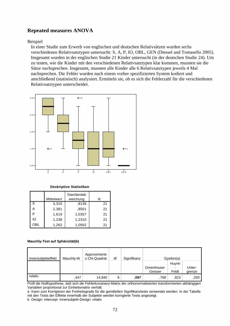
Repeated measures ANOVA

BeispielIn einer Studie zum Erwerb von englischen und deutschen Relativsätzen wurden sechs verschiedenen Relativsatztypen untersucht: S, A, P, IO, OBL, GEN (Diessel and Tomasello 2005). Insgesamt wurden in der englischen Studie 21 Kinder untersucht (in der deutschen Studie 24). Um zu testen, wie die Kinder mit den verschiedenen Relativsatztypen klar kommen, mussten sie die Sätze nachsprechen. Insgesamt, mussten alle Kinder alle 6 Relativsatztypen jeweils 4 Mal nachsprechen. Die Fehler wurden nach einem vorher spezifizierten System kodiert und anschließend (statistisch) analysiert. Ermitteln sie, ob es sich die Fehlerzahl für die verschiedenen Relativsatztypen unterscheidet.

S A P IO O B L G E N

0,0

1,0

2,0

3,0

4,0

2 1

1 3

1 0

Deskriptive Statistiken

3,310 ,8136 212,381 ,8501 211,619 1,0357 211,238 1,2310 211,262 1,0562 21

SAPIOOBL

MittelwertStandardabweichung N

Mauchly-Test auf Sphärizität(b)

Innersubjekteffekt Mauchly-WApproximiertes Chi-Quadrat df Signifikanz Epsilon(a)

Greenhouse-Geisser

Huynh-

FeldtUnter-grenze

relativ ,447 14,840 9 ,097 ,768 ,923 ,250

Prüft die Nullhypothese, daß sich die Fehlerkovarianz-Matrix der orthonormalisierten transformierten abhängigen Variablen proportional zur Einheitsmatrix verhält.a Kann zum Korrigieren der Freiheitsgrade für die gemittelten Signifikanztests verwendet werden. In der Tabelle mit den Tests der Effekte innerhalb der Subjekte werden korrigierte Tests angezeigt.b Design: Intercept Innersubjekt-Design: relativ

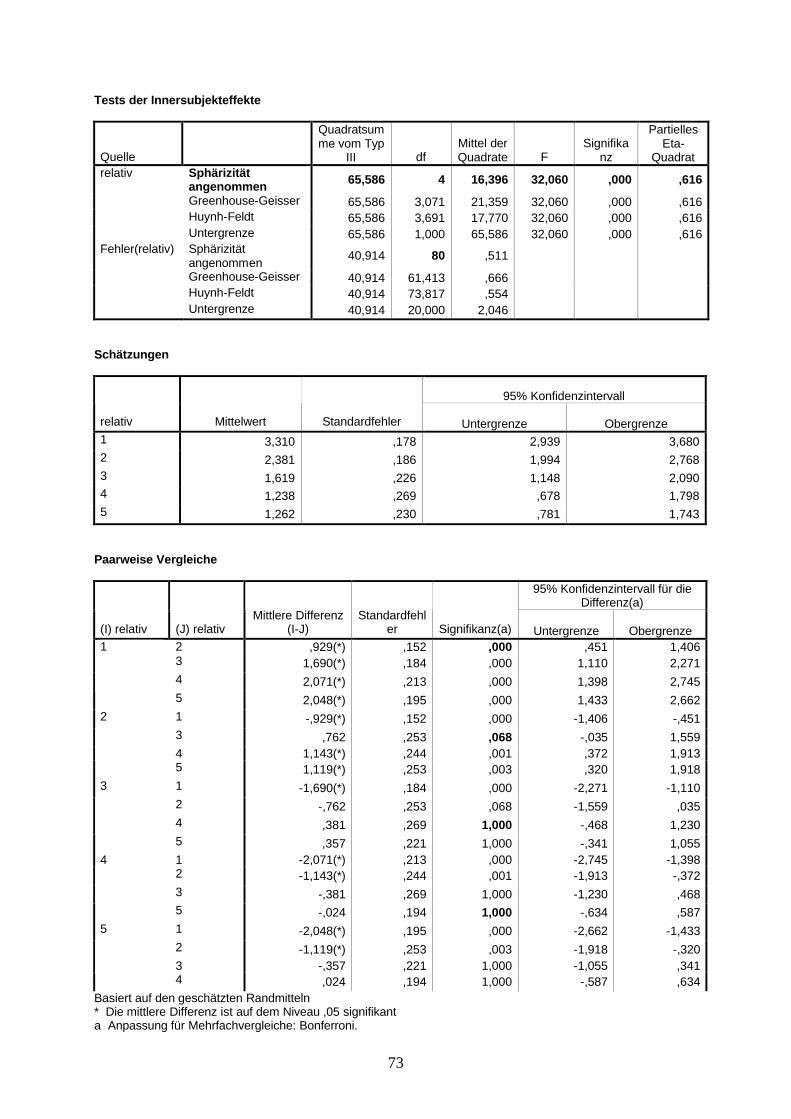
73

Tests der Innersubjekteffekte

Quelle

Quadratsumme vom Typ

III dfMittel der Quadrate F

Signifikanz

Partielles Eta-

Quadratrelativ Sphärizität

angenommen 65,586 4 16,396 32,060 ,000 ,616

Greenhouse-Geisser 65,586 3,071 21,359 32,060 ,000 ,616Huynh-Feldt 65,586 3,691 17,770 32,060 ,000 ,616Untergrenze 65,586 1,000 65,586 32,060 ,000 ,616

Fehler(relativ) Sphärizität angenommen 40,914 80 ,511

Greenhouse-Geisser 40,914 61,413 ,666Huynh-Feldt 40,914 73,817 ,554Untergrenze 40,914 20,000 2,046

Schätzungen

95% Konfidenzintervall

relativ Mittelwert Standardfehler Untergrenze Obergrenze1 3,310 ,178 2,939 3,6802 2,381 ,186 1,994 2,7683 1,619 ,226 1,148 2,0904 1,238 ,269 ,678 1,7985 1,262 ,230 ,781 1,743

Paarweise Vergleiche

95% Konfidenzintervall für die Differenz(a)

(I) relativ (J) relativMittlere Differenz

(I-J)Standardfehl

er Signifikanz(a) Untergrenze Obergrenze2 ,929(*) ,152 ,000 ,451 1,4063 1,690(*) ,184 ,000 1,110 2,2714 2,071(*) ,213 ,000 1,398 2,745

1

5 2,048(*) ,195 ,000 1,433 2,6622 1 -,929(*) ,152 ,000 -1,406 -,451

3 ,762 ,253 ,068 -,035 1,5594 1,143(*) ,244 ,001 ,372 1,9135 1,119(*) ,253 ,003 ,320 1,918

3 1 -1,690(*) ,184 ,000 -2,271 -1,1102 -,762 ,253 ,068 -1,559 ,0354 ,381 ,269 1,000 -,468 1,2305 ,357 ,221 1,000 -,341 1,055

4 1 -2,071(*) ,213 ,000 -2,745 -1,3982 -1,143(*) ,244 ,001 -1,913 -,3723 -,381 ,269 1,000 -1,230 ,4685 -,024 ,194 1,000 -,634 ,587

5 1 -2,048(*) ,195 ,000 -2,662 -1,4332 -1,119(*) ,253 ,003 -1,918 -,3203 -,357 ,221 1,000 -1,055 ,3414 ,024 ,194 1,000 -,587 ,634

Basiert auf den geschätzten Randmitteln* Die mittlere Differenz ist auf dem Niveau ,05 signifikanta Anpassung für Mehrfachvergleiche: Bonferroni.

74


Gepaarte Differenzen95%

Konfidenzintervall der Differenz

Mittelwert

Standardabweichun

g

Standardfehler des Mittelwert

es Untere Obere T dfSig. (2-seitig)

Paaren 1

S - A ,9286 ,6944 ,1515 ,6125 1,2446 6,128 20 ,000

Paaren 2

A - P ,7619 1,1578 ,2527 ,2349 1,2889 3,016 20 ,007

Paaren 3

P - IO ,3810 1,2339 ,2693 -,1807 ,9426 1,415 20 ,173

Paaren 4

IO -OBL -,0238 ,8871 ,1936 -,4276 ,3800 -,123 20 ,903

Friedman’s ANOVA

BeispielEin Linguist möchte wissen, ob sich die Stellung von Adverbialsätzen mit ihrer Bedeutung verändert. Dafür untersucht er die Adverbialsätze von 15 Personen in Transkriptionen gesprochener Sprache. Die Adverbialsätze werden in drei große semantische Klassen eingeteilt: (1) Konditionalsätze, (2) Temporalsätze, (3) Kausalsätze. Für jede Klasse wurde ermittelt, wie häufig ein Sprecher den Satz jeweils vor und nach dem Hauptsatz verwendethat. Eingeschobene Adverbialsätze, die ohnehin nur sehr selten vorkommen, wurden ignoriert.

Konditional Kausal TemporalVor Nach Vor Nach Vor Nach

123456789101112131415

42,7072,7075,0063,6088,9070,0072,7060,0066,7064,0057,1045,5070,60100,0055,50

57,3027,3025,0036,6011,1030,0027,3040,0033,3036,0042,9054,5029,40,00

45,50

12,509,10,00

20,00,00,00,00

37,50,00,00

10,0023,1033,30,007,70

87,5090,90100,0080,00100,00100,00100,0062,50100,00100,0090,0076,9066,70100,0092,30

28,1036,6026,7010,3041,7036,0056,0028,6052,6015,4010,9026,2066,6041,7034,30

71,9063,4073,3089,7058,3064,0044,0071,4047,4084,6089,1073,8033,4058,3065,70

75

Ränge

Mittlerer RangConditional 3,00Causal 1,13Temporal 1,87

Statistik für Testa

1526,533

2,000

NChi-QuadratdfAsymptotische Signifikanz

Friedman-Testa.


Causal -Conditional

Z -3,408(a)Asymptotische Signifikanz (2-seitig) ,001

a Basiert auf positiven Rängen.b Wilcoxon-Test


Temporal -Conditional

Z -3,408(a)Asymptotische Signifikanz (2-seitig) ,001

a Basiert auf positiven Rängen.b Wilcoxon-Test


-3,011a

,003

ZAsymptotischeSignifikanz (2-seitig)

Temporal -Causal

Basiert auf negativen Rängen.a.

Wilcoxon-Testb.

Conditional-Causal

Conditional-Temporal

Causal-Temporal

76

Multifactorial ANOVA

In einem faktorial Design untersucht man einmal den Effekt jeder einzelnen IV (main effects) und zum anderen die Interaktionen zwischen den beiden IVs (interaction). Außerdem werden für jede IV die Effekte berechnet, die erzielt werden, wenn man dieanderen IV auf einem bestimmten Level konstant hält (simple main effects).

Animacy

Type of NP Inanimate Animate averageLexical 00 10 5Pronominal 20 30 25average 10 20 15

0

5

10

15

20

25

30

35

Inanimate Animate

LexicalPronominal

Main Effect beschreibt den Unterschied zwischen den beiden Levels der beiden IVs:1. Main Effect (NP type): 25 – 5 = 20 2. Main Effect (Syntactic Function): 20 – 10 = 10

Simple Main Effect beschreibt den Effekt eines bestimmten Faktors, auf einem bestimmten Level des anderen Faktors. Bei einem 22 Design gibt es 4 Simple Main Effects:

1. Wenn wir uns nur die Subjekte anschauen, dann sind pronominale NPs um 20 Punkte häufiger als lexikalische NPs: 20 – 0 = 20.

2. Wenn wir uns nur die Objekte anschauen, dann sind pronominale NPs auch um 20 Punkte häufiger als lexikalische NPs: 30 – 10 = 20.

3. Wenn wir uns nur Lexikalische NPs anschauen, dann sind Objekte um 10 Punkte häufiger als Subjekte: 30 – 20 = 10.

4. Wenn wir uns nur pronominale NPs anschauen, dann sind Objekte auch um 10 Punkte häufiger als Subjekte: 10 – 0 = 10.

Interaction: Wenn die Simple Main Effects auf den beiden Levels der anderen IV konstant bleiben, dann gibt es zwischen den beiden IVs keine Interaktion.

77

Graphische Darstellung der Simple Main Effects

Animacy

Type of NP Inanimate Animate averageLexical 00 10 5Pronominal 20 40 25average 10 25 17.5

0

5

10

15

20

25

30

35

40

45

Inanimate Animate

LexicalPronominal

0

5

10

15

20

25

30

35

0 0,5 1 1,5 2 2,5

LexicalPronominal

0

5

10

15

20

25

30

35

0 0,5 1 1,5 2 2,5

LexicalPronominal

0

5

10

15

20

25

30

35

0 0,5 1 1,5 2 2,5

LexicalPronominal

0

5

10

15

20

25

30

35

0 0,5 1 1,5 2 2,5

LexicalPronominal

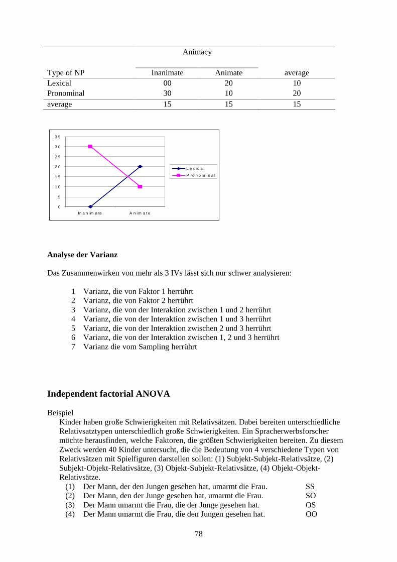
78

Animacy

Type of NP Inanimate Animate averageLexical 00 20 10Pronominal 30 10 20average 15 15 15

0

5

1 0

1 5

2 0

2 5

3 0

3 5

In a n im a te A n im a t e

L e x i c a l

P ro n o m in a l

Analyse der Varianz

Das Zusammenwirken von mehr als 3 IVs lässt sich nur schwer analysieren:

1 Varianz, die von Faktor 1 herrührt2 Varianz, die von Faktor 2 herrührt3 Varianz, die von der Interaktion zwischen 1 und 2 herrührt4 Varianz, die von der Interaktion zwischen 1 und 3 herrührt5 Varianz, die von der Interaktion zwischen 2 und 3 herrührt6 Varianz, die von der Interaktion zwischen 1, 2 und 3 herrührt7 Varianz die vom Sampling herrührt

Independent factorial ANOVA

BeispielKinder haben große Schwierigkeiten mit Relativsätzen. Dabei bereiten unterschiedliche Relativsatztypen unterschiedlich große Schwierigkeiten. Ein Spracherwerbsforscher möchte herausfinden, welche Faktoren, die größten Schwierigkeiten bereiten. Zu diesem Zweck werden 40 Kinder untersucht, die die Bedeutung von 4 verschiedene Typen von Relativsätzen mit Spielfiguren darstellen sollen: (1) Subjekt-Subjekt-Relativsätze, (2) Subjekt-Objekt-Relativsätze, (3) Objekt-Subjekt-Relativsätze, (4) Objekt-Objekt-Relativsätze.

(1) Der Mann, der den Jungen gesehen hat, umarmt die Frau. SS(2) Der Mann, den der Junge gesehen hat, umarmt die Frau. SO(3) Der Mann umarmt die Frau, die der Junge gesehen hat. OS(4) Der Mann umarmt die Frau, die den Jungen gesehen hat. OO

79

In der Literatur gibt es zwei Hypothesen, die in diesem Zusammenhang von Interesse sind: (a) die Non-Interruption-Hypothesis, die besagt, dass Relativsätze, die dem Hauptsatz folgen, weniger Schwierigkeiten bereiten, als Relativsätze, die in den Hauptsatz eingebetet sind (OS+OO einfacher als SS+SO); (b) die Parallel-Function-Hypothesis, die besagt, dass Relativsätze, in denen der Kopf des Relativsatzes und das Relativpronomen die gleiche syntaktische Funktion haben, leichter zu verstehen sind als Relativsätze, in denen der Kopf des Relativsatzes und das Relativpronomen unterschiedliche syntaktische Funktionen haben (SS+OO einfacher als SO+OS). Die folgende Tabelle zeigt die Anzahl der Fehler, die die Kinder bei der Darstellung der vier Relativsatztypen gemacht haben. Die 40 Kinder wurden in vier Gruppen aufgeteilt und jedes Kind hat jeweils 15 Relativsätze eines bestimmten Typs nachgespielt. Zusammen mit den Relativsätzen mussten die Kinder 30 Distraktoren nachspielen. Die folgende Tabelle zeigt die Anzahl der Fehler.

Subjekt-Kopf Objekt-KopfSubjekt-Pronomen 4,5

4,565

5,54,54

6,577

0111

1,51,51,522

1,5Objekt-Pronomen 11

10119

10,510,59,579

10

13,55,53,544444

4,5

SS 1:1 OS 2:1SO 1:2 OO 2:2

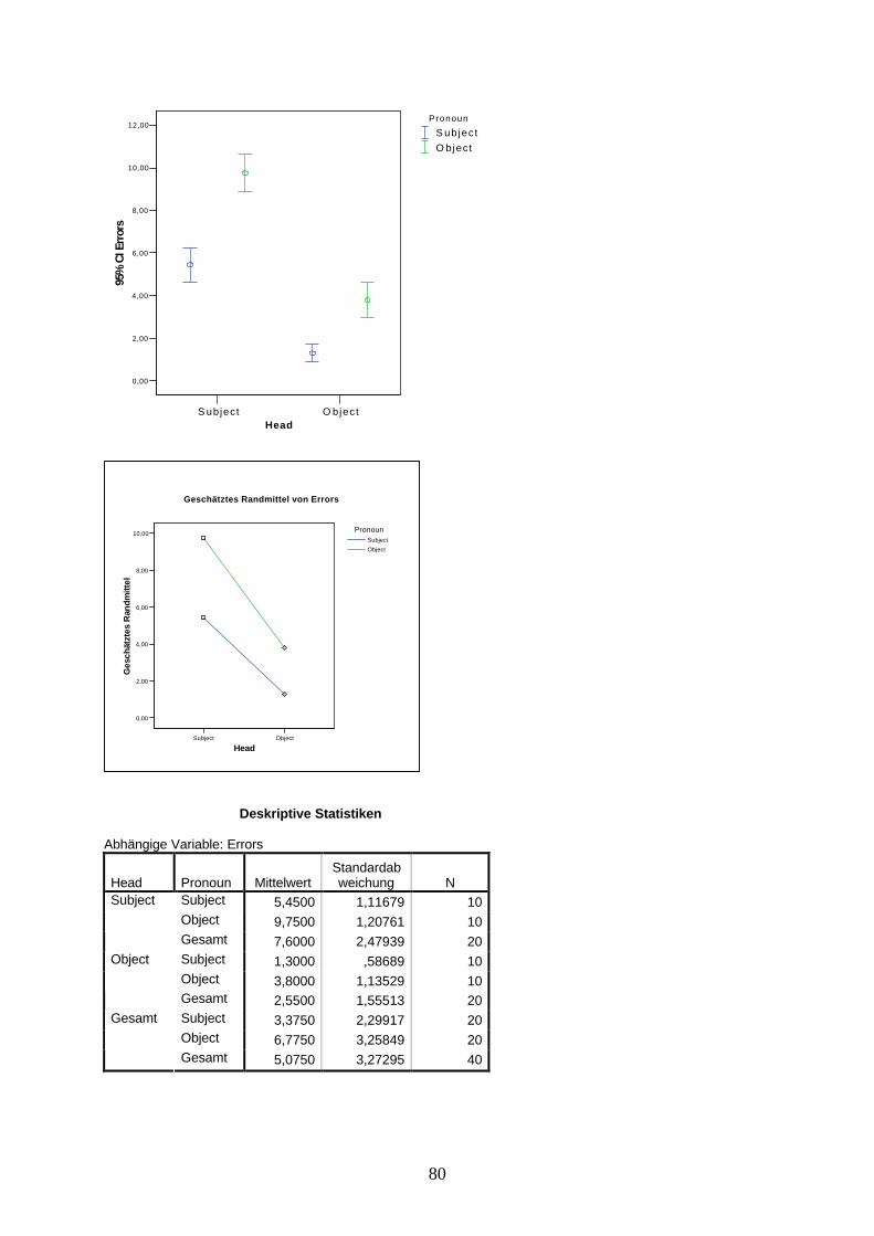
80

S ubject O bjectHead

0,00

2,00

4,00

6,00

8,00

10,00

12,0095

% C

I Err

ors

Pronoun

S ubjec tO bject

Deskriptive Statistiken

Abhängige Variable: Errors

Head Pronoun MittelwertStandardabweichung N

Subject 5,4500 1,11679 10Object 9,7500 1,20761 10

Subject

Gesamt 7,6000 2,47939 20Subject 1,3000 ,58689 10Object 3,8000 1,13529 10

Object

Gesamt 2,5500 1,55513 20Subject 3,3750 2,29917 20Object 6,7750 3,25849 20

Gesamt

Gesamt 5,0750 3,27295 40

Subject Object

Head

0,00

2,00

4,00

6,00

8,00

10,00

Ges

chät

ztes

Ran

dmitt

el

PronounSubjectObject

Geschätztes Randmittel von Errors

81

Tests der Zwischensubjekteffekte

Abhängige Variable: Errors

QuelleQuadratsumme vom Typ III df

Mittel der Quadrate F Signifikanz

Partielles Eta-Quadrat

Korrigiertes Modell 378,725(a) 3 126,242 116,382 ,000 ,907Konstanter Term 1030,225 1 1030,225 949,759 ,000 ,963Head 255,025 1 255,025 235,106 ,000 ,867Pronoun 115,600 1 115,600 106,571 ,000 ,747Head * Pronoun 8,100 1 8,100 7,467 ,010 ,172Fehler 39,050 36 1,085Gesamt 1448,000 40Korrigierte Gesamtvariation 417,775 39

a R-Quadrat = ,907 (korrigiertes R-Quadrat = ,899)

Planned comparisons:

Test bei unabhängigen Stichprobena

,031 ,862 -8,267 18 ,000 -4,30000 ,52015 -5,39279 -3,20721

-8,267 17,891 ,000 -4,30000 ,52015 -5,39327 -3,20673

Varianzen sind gleichVarianzen sind nichtgleich

ErrorsF Signifikanz

Levene-Test derVarianzgleichheit

T df Sig. (2-seitig)Mittlere

DifferenzStandardfehler der Differenz Untere Obere


T-Test für die Mittelwertgleichheit

Head = Subjecta.


,637 ,435 -6,186 18 ,000 -2,50000 ,40415 -3,34908 -1,65092

-6,186 13,490 ,000 -2,50000 ,40415 -3,36989 -1,63011


ErrorsF Signifikanz






Head = Objecta.


6,959 ,017 10,402 18 ,000 4,15000 ,39896 3,31182 4,98818

10,402 13,619 ,000 4,15000 ,39896 3,29207 5,00793


ErrorsF Signifikanz






Pronoun = Subjecta.


,363 ,554 11,352 18 ,000 5,95000 ,52414 4,84882 7,05118

11,352 17,932 ,000 5,95000 ,52414 4,84852 7,05148


ErrorsF Signifikanz






Pronoun = Objecta.

82

Paired factorial ANOVA

BeispielDas gleiche Experiment kann natürlich auch mit einem within-subjects Design durchgeführt werden. Dazu müssen die Daten jedoch anders eingegeben werden.

SS SO OS OO12345678910

4,54,565

5,54,54

6,577

1110119

10,510,59,579

10

0111

1,51,51,522

1,5

13,55,53,544444

4,5

Mauchly-Test auf Sphärizitätb

Maß: MASS_1

1,000 ,000 0 . 1,000 1,000 1,0001,000 ,000 0 . 1,000 1,000 1,0001,000 ,000 0 . 1,000 1,000 1,000

Innersubjekteffektheadprohead * pro

Mauchly-WApproximiertes Chi-Quadrat df Signifikanz

Greenhouse-Geisser Huynh-Feldt Untergrenze

Epsilona

Prüft die Nullhypothese, daß sich die Fehlerkovarianz-Matrix der orthonormalisierten transformierten abhängigen Variablenproportional zur Einheitsmatrix verhält.

Kann zum Korrigieren der Freiheitsgrade für die gemittelten Signifikanztests verwendet werden. In der Tabelle mitden Tests der Effekte innerhalb der Subjekte werden korrigierte Tests angezeigt.

a.

Design: Intercept Innersubjekt-Design: head+pro+head*pro

b.

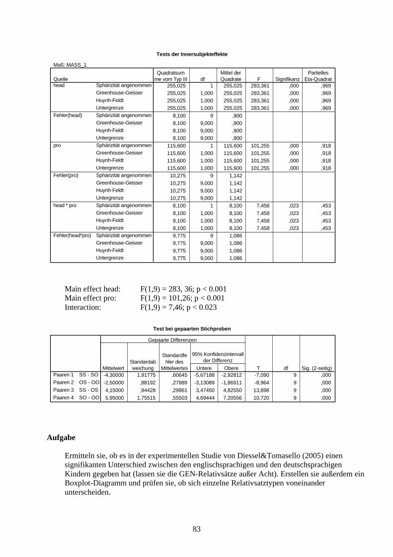
83

Tests der Innersubjekteffekte

Maß: MASS_1

255,025 1 255,025 283,361 ,000 ,969255,025 1,000 255,025 283,361 ,000 ,969255,025 1,000 255,025 283,361 ,000 ,969255,025 1,000 255,025 283,361 ,000 ,969

8,100 9 ,9008,100 9,000 ,9008,100 9,000 ,9008,100 9,000 ,900

115,600 1 115,600 101,255 ,000 ,918115,600 1,000 115,600 101,255 ,000 ,918115,600 1,000 115,600 101,255 ,000 ,918115,600 1,000 115,600 101,255 ,000 ,91810,275 9 1,14210,275 9,000 1,14210,275 9,000 1,14210,275 9,000 1,1428,100 1 8,100 7,458 ,023 ,4538,100 1,000 8,100 7,458 ,023 ,4538,100 1,000 8,100 7,458 ,023 ,4538,100 1,000 8,100 7,458 ,023 ,4539,775 9 1,0869,775 9,000 1,0869,775 9,000 1,0869,775 9,000 1,086

Sphärizität angenommenGreenhouse-GeisserHuynh-FeldtUntergrenzeSphärizität angenommenGreenhouse-GeisserHuynh-FeldtUntergrenzeSphärizität angenommenGreenhouse-GeisserHuynh-FeldtUntergrenzeSphärizität angenommenGreenhouse-GeisserHuynh-FeldtUntergrenzeSphärizität angenommenGreenhouse-GeisserHuynh-FeldtUntergrenzeSphärizität angenommenGreenhouse-GeisserHuynh-FeldtUntergrenze

Quellehead

Fehler(head)

pro

Fehler(pro)

head * pro

Fehler(head*pro)

Quadratsumme vom Typ III df


PartiellesEta-Quadrat

Main effect head: F(1,9) = 283, 36; p < 0.001Main effect pro: F(1,9) = 101,26; p < 0.001Interaction: F(1,9) = 7,46; p < 0.023


-4,30000 1,91775 ,60645 -5,67188 -2,92812 -7,090 9 ,000-2,50000 ,88192 ,27889 -3,13089 -1,86911 -8,964 9 ,0004,15000 ,94428 ,29861 3,47450 4,82550 13,898 9 ,0005,95000 1,75515 ,55503 4,69444 7,20556 10,720 9 ,000

SS - SOPaaren 1OS - OOPaaren 2SS - OSPaaren 3SO - OOPaaren 4

MittelwertStandardabweichung

Standardfehler des

Mittelwertes Untere Obere


Gepaarte Differenzen

T df Sig. (2-seitig)

Aufgabe

Ermitteln sie, ob es in der experimentellen Studie von Diessel&Tomasello (2005) einen signifikanten Unterschied zwischen den englischsprachigen und den deutschsprachigen Kindern gegeben hat (lassen sie die GEN-Relativsätze außer Acht). Erstellen sie außerdem ein Boxplot-Diagramm und prüfen sie, ob sich einzelne Relativsatztypen voneinander unterscheiden.

empirical methods of linguistics research - …x4diho/script empirical methods... · 2007-10-17 ·...

Documents