empirical mo deling of extreme ev - statistics.berkeley.edu
TRANSCRIPT

Empirical Modeling of Extreme Events from Return{VolumeTime Series in Stock Market
Peter B�uhlmann �
Department of Statistics
University of California BerkeleyBerkeley, CA 94720-3860
June 1996
Abstract
We propose the discretization of real-valued �nancial time series into few ordinalvalues and use non-linear likelihood modeling for sparse Markov chains within theframework of generalized linear models for categorical time series.
We analyze daily return and volume data and estimate the probability structureof the process of extreme lower, extreme upper and the complementary usual events.Knowing the whole probability law of such ordinal-valued vector processes of extremeevents of return and volume allows us to quantify non-linear associations. In particu-lar, we �nd a (new kind of) asymmetry in the return{volume relationship which is apartial answer to a research issue given by Karpo� (1987).
We also propose a simple prediction algorithm which is based on an empiricallyselected model.
Keywords: Asymmetric volume{return relation; Finance; Generalized linear model; Markov
chain; Non-linear association; Prediction
�Research supported in part by the Swiss National Science Foundation.
1

1 Introduction
Many of the time series occurring in �nance su�er from the fact that there are no simplemechanistic models which substantially reduce the complexity of the data and still explainit well. Either the models are too simple to explain the nature of �nancial phenomena orthe model is too complex so that over-�tting occurs. Over-�tting results in high variabilityof estimates and reproducibility in a similar situation cannot be satisfactorily achieved.
If we believe in an intrinsic high complexity of the �nancial nature, we seem to beforced to work with models having many parameters and hence with estimates being highlyvariable. We propose one way out of this impasse by the following question: Why modelingthe whole structure of an observed �nancial time series, rather than modeling only somestructure, such as extreme events? We propose here a discretization of a real-valued�nancial time series into only three ordinal categories, corresponding to extreme lower,extreme upper and the complementary (usual) events. This results in a huge reduction ofthe number of parameters for a model and still allows to explore questions about extremeevents, such as unusual values or large positive or negative increments.
We exemplify the method by analyzing daily data of return from the Dow Jones indexand volume from the New York Stock Exchange (NYSE). For analyzing the three events(lower extreme, upper extreme and usual) we use a likelihood modeling approach basedon a higher order Markovian assumption, and model cumulative probabilities within theframework of generalized linear models with lagged variables treated as factors. Theword `linear' can be misleading, our model class is very general and broad, since we aretreating lagged variables as factors. This then includes processes similar to arbitrary �niteorder Markov chains. By putting a natural hierarchy on such models we typically modelsparse rather than full Markov chains, which allows to avoid the curse of dimensionality,cf. section 3.1. Such models are very exible, one can also include continuous covariatesand explanatory exogenous factors for describing the dynamics. For a good overview inthe independent set-up, cf. McCullagh and Nelder (1989). Within this model class, theselection of a model can be supported by considering measures of predictive power suchas Akaike's information criterion (AIC), cf. Akaike (1973). Having selected a model, wealso propose a simple prediction algorithm.
By discretizing we pay a price by restricting the focus to extreme events (and thecomplementary usual events). On the other hand we gain a lot in the process of empiricalmodel searching and �tting. Moreover, our conclusions are probabilistic statements ratherthan the often used correlation which measures only linear association.
We obtain by our method fully probabilistic interpretations for the relationship ofextreme events of return from the Dow Jones and volume from the NYSE. This gives newinsight into the structure of �nancial markets. In particular, our empirical results are ananswer to a research question posed by Karpo� (1987): for our data, the volume{returnrelationship, at least for extreme events, is in a new sense asymmetric.
This paper is organized as follows. In section 2 we describe the data set, in section 3we explain the modeling and prediction techniques, in section 4 we report our empirical�ndings for the analyzed data set, in section 5 we draw some conclusions and in section 6we brie y outline some more mathematical and computational details.
2

2 The data
The data is about daily return of the Dow Jones index and daily volume of the New YorkStock Exchange (NYSE). The daily measurements are from the period July 1962 throughJune 1988, corresponding to 6430 days 2. What we term `volume' is the standardizedaggregate turnover on the NYSE,
Volt = log(Ft)� log(t�1X
s=t�100
Fs=100);
where Fs equals the fraction of shares traded on day s.The return is de�ned as
Rett = log(Dt)� log(Dt�1);
where Dt is the index of the Dow Jones on day t. This is the same data with the samestandardization as in Weigend and LeBaron (1994). Figure 1 shows these standardized�nancial time series; the time t=6253, where return Rett < �0:2 corresponds to the 1987crash. Besides this special structure around the crash, both series look quite stationary.
3 Modeling
Since mechanistic theories for volume or return are not broadly accepted, we want to usea modeling approach which is in a nonparametric spirit. Our models in sections 3.3 and3.4 can easily be extended to include some usual parametric parts, yielding then a kind ofsemiparametric model.
3.1 The curse of dimensionality for full Markov chains
The most natural model for a stationary process fXtgt2ZZ (Xt 2 IR), assuming no particularunderlying mechanistic system, is maybe a full Markov chain of order p, i.e.,
IP[Xt � xjXt�1; Xt�2; : : :] = IP[Xt � xjXt�1; : : : ; Xt�p]; x 2 IR; 1 � p <1:
This implies the only implicit assumption, namely that the process fXtgt2ZZ has a �nitememory of length p.
Such models are very general and usually too complex. Even if Xt would only takevalues in a �nite space S of cardinality jSj, these models involve jSjp+1�1 free parametersto estimate. For example, jSj = 5; p = 5 yields 15624 free parameters, which is prohibitive!Such an explosion of parameters corresponds to a space which is very hard to cover withdata points. This phenomenon is called the curse of dimensionality.
We learn that full Markov chains with values in a space S with about jSj � 4 do oftennot yield a big reduction of the complexity in the data, unless the sample size is huge.
2This data is publicly available via the internet:http://ssdc.ucsd.edu/ssdc/NYSE.Date.Day.Return.Volume.Vola.text
3
3.2 Discretizing into ordinal values
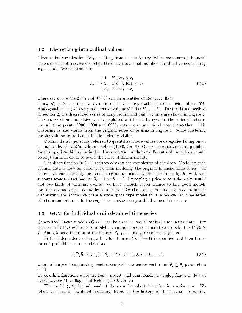
Given a single realization Ret1; : : : ;Retn from the stationary (which we assume), �nancialtime series of returns, we discretize the data into a small number of ordinal values yieldingR1; : : : ; Rn. We propose here
Rt =
8<:1; if Rett � c12; if c1 < Rett � c23; if Rett > c2
; (3.1)
where c1; c2 are the 2.5% and 97.5% sample quantiles of Ret1; : : : ;Retn.Thus, Rt 6= 2 describes an extreme event with expected occurrence being about 5%.Analogously as in (3.1) we can discretize volume yielding V1; : : : ; Vn. For the data describedin section 2, the discretized series of daily return and daily volume are shown in Figure 2.The more extreme activities can be exploited a little bit by eye: for the series of returnsaround time points 3000, 5000 and 6200, extreme events are clustered together. Thisclustering is also visible from the original series of returns in Figure 1. Some clusteringfor the volume series is also but less clearly visible.
Ordinal data is generally referred to quantities whose values are categories falling on anordinal scale, cf. McCullagh and Nelder (1989, Ch. 5). Other discretizations are possible,for example into binary variables. However, the number of di�erent ordinal values shouldbe kept small in order to avoid the curse of dimensionality.
The discretization in (3.1) reduces already the complexity of the data. Modeling suchordinal data is now an easier task than modeling the original �nancial time series. Ofcourse, we can now only say something about `usual events', described by Rt = 2, andextreme events, described by Rt = 1 or Rt = 3. By paying a price to consider only `usual'and two kinds of `extreme events', we have a much better chance to �nd good modelsfor such ordinal data. We address in section 3.6 the issue about loosing information bydiscretizing and introduce there a state space type model for the real-valued time seriesof return and volume. In the sequel we consider only ordinal-valued time series.
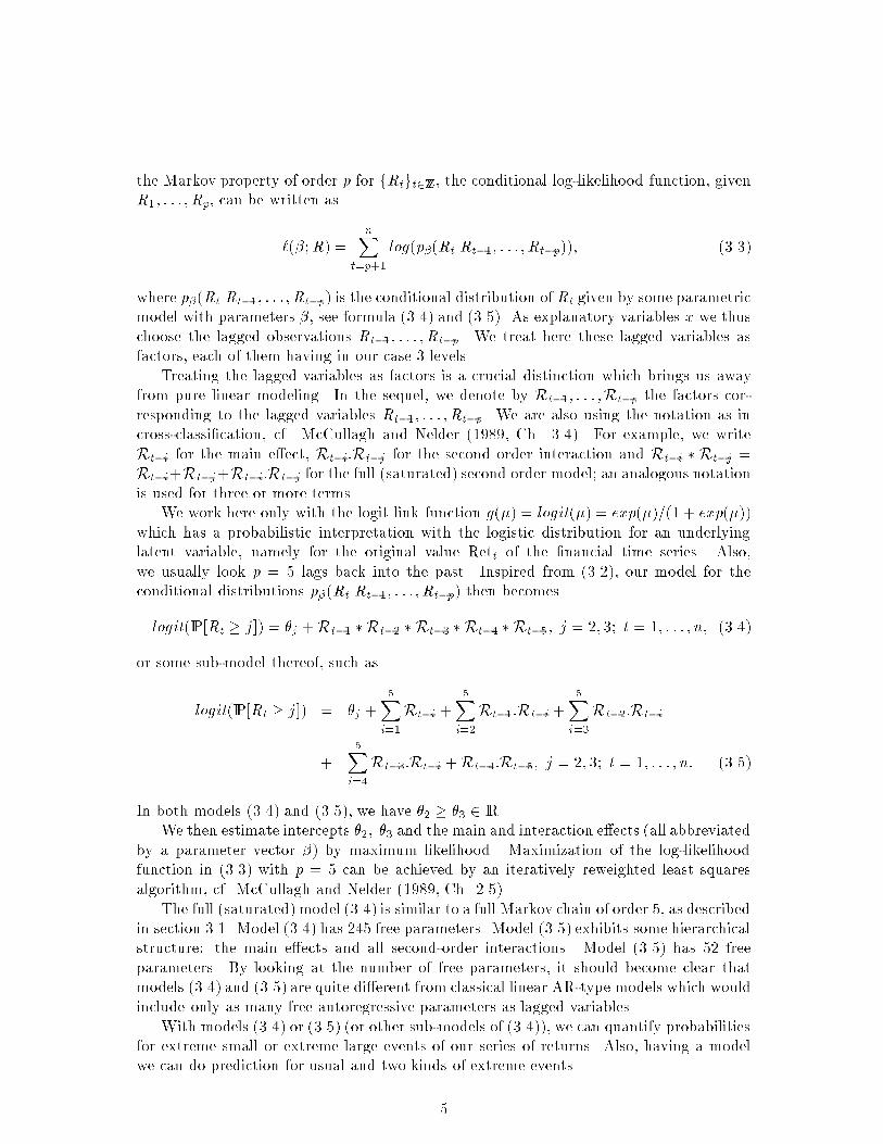
3.3 GLM for individual ordinal-valued time series
Generalized linear models (GLM) can be used to model ordinal time series data. Fordata as in (3.1), the idea is to model the complementary cumulative probabilities IP[Rt �
j] (j = 2; 3) as a function of the history Rt�1; : : : ; Rt�p for some 1 � p <1.
In the independent set-up, a link function g : (0; 1) ! IR is speci�ed and then trans-formed probabilities are modeled as
g(IP[Rt � jjx]) = �j + x0�; j = 2; 3; t = 1; : : : ; n; (3.2)
where x is a p� 1 explanatory vector, � a p� 1 parameter vector and �2 � �3 parametersin IR.Typical link functions g are the logit-, probit- and complementary loglog-function. For anoverview, see McCullagh and Nelder (1989, Ch. 5).
The model (3.2) for independent data can be adapted to the time series case. Wefollow the idea of likelihood modeling, based on the history of the process. Assuming
4
the Markov property of order p for fRtgt2ZZ, the conditional log-likelihood function, givenR1; : : : ; Rp, can be written as
`(�;R) =nX
t=p+1
log(p�(RtjRt�1; : : : ; Rt�p)); (3.3)
where p�(RtjRt�1; : : : ; Rt�p) is the conditional distribution of Rt given by some parametricmodel with parameters �, see formula (3.4) and (3.5). As explanatory variables x we thuschoose the lagged observations Rt�1; : : : ; Rt�p. We treat here these lagged variables asfactors, each of them having in our case 3 levels.
Treating the lagged variables as factors is a crucial distinction which brings us awayfrom pure linear modeling. In the sequel, we denote by Rt�1; : : : ;Rt�p the factors cor-responding to the lagged variables Rt�1; : : : ; Rt�p. We are also using the notation as incross-classi�cation, cf. McCullagh and Nelder (1989, Ch. 3.4). For example, we writeRt�i for the main e�ect, Rt�i:Rt�j for the second order interaction and Rt�i � Rt�j =Rt�i+Rt�j+Rt�i:Rt�j for the full (saturated) second order model; an analogous notationis used for three or more terms.
We work here only with the logit link function g(�) = logit(�) = exp(�)=(1 + exp(�))which has a probabilistic interpretation with the logistic distribution for an underlyinglatent variable, namely for the original value Rett of the �nancial time series. Also,we usually look p = 5 lags back into the past. Inspired from (3.2), our model for theconditional distributions p�(RtjRt�1; : : : ; Rt�p) then becomes
logit(IP[Rt � j]) = �j +Rt�1 � Rt�2 � Rt�3 � Rt�4 � Rt�5; j = 2; 3; t = 1; : : : ; n; (3.4)
or some sub-model thereof, such as
logit(IP[Rt � j]) = �j +5X
i=1
Rt�i +5X
i=2
Rt�1:Rt�i +5X
i=3
Rt�2:Rt�i
+5X
i=4
Rt�3:Rt�i +Rt�4:Rt�5; j = 2; 3; t = 1; : : : ; n: (3.5)
In both models (3.4) and (3.5), we have �2 � �3 2 IR.We then estimate intercepts �2; �3 and the main and interaction e�ects (all abbreviated
by a parameter vector �) by maximum likelihood. Maximization of the log-likelihoodfunction in (3.3) with p = 5 can be achieved by an iteratively reweighted least squaresalgorithm, cf. McCullagh and Nelder (1989, Ch. 2.5).
The full (saturated) model (3.4) is similar to a full Markov chain of order 5, as describedin section 3.1. Model (3.4) has 245 free parameters. Model (3.5) exhibits some hierarchicalstructure: the main e�ects and all second-order interactions. Model (3.5) has 52 freeparameters. By looking at the number of free parameters, it should become clear thatmodels (3.4) and (3.5) are quite di�erent from classical linear AR-type models which wouldinclude only as many free autoregressive parameters as lagged variables.
With models (3.4) or (3.5) (or other sub-models of (3.4)), we can quantify probabilitiesfor extreme small or extreme large events of our series of returns. Also, having a modelwe can do prediction for usual and two kinds of extreme events.
5

3.4 Joint GLM for two ordinal-valued time series
There is a substantial interest to quantify the dependence or association between returnand volume, cf. Karpo� (1987). Most of the previous work was done by looking atcross-correlations, a measure for linear dependence. We will develop here joint likelihoodmodeling, resulting in estimates for the joint probability of discretized return and dis-cretized volume. In other words, we will track down the ultimate aim in this set-up,namely the knowledge of the whole probability structure for usual and extreme events ofreturn and volume.
As in (3.1) we discretize return and volume into 3 ordinal values, yielding R1; : : : ; Rn
for discretized return and V1; : : : ; Vn for discretized volume. We study �rst the relationshipof return given volume, according to a Wall Street saying that `it takes volume to makeprices move'. This means that Rt should depend on Vt for the same time point t.
For likelihood modeling, we again assume the Markov property of order p for theordinal-vector process f(Rt; Vt)
0gt2ZZ. The log-likelihood function, conditional onR1; : : : ; Rp,V1; : : : ; Vp, then becomes
`(�;R; V ) =nX
t=p+1
log(p�(Rt; VtjRt�1; Vt�1; : : : ; Rt�p; Vt�p))
=nX
t=p+1
log(p�R(RtjVt; Rt�1; Vt�1; : : : ; Rt�p; Vt�p))
+nX
t=p+1
log(p�V (VtjRt�1; Vt�1; : : : ; Rt�p; Vt�p))
= `(�R;R; V ) + `(�V ;R; V ); (3.6)
where the p�(:j:)'s are the conditional probabilities given by some parametric model withparameters � as in formula (3.7).
We thus introduce an explanatory factor Vt with 3 levels corresponding to the vari-able Vt. Additionally, the factors for the lagged variables are denoted by Rt�i and Vt�i(i=1,: : : ,5). Similarly as in models (3.4) and (3.5) we model
logit(IP[Rt � j]) = �Rj + Vt +5X
i=1
Rt�i +5X
i=2
Rt�1:Rt�i +5X
i=3
Rt�2:Rt�i
+5X
i=4
Rt�3:Rt�i +Rt�4:Rt�5;
logit(IP[Vt � j]) = �Vj +5X
i=1
Vt�i +5X
i=1
Rt�i; j = 2; 3; t = 1; : : : ; n; (3.7)
where �R2 � �R3 ; �V2 � �V3 .
Of course, other models than (3.7) are possible. In particular, the model for IP[Vt � j]could be thought to be without the factors Rt�i (i = 1; : : : ; 5). Model (3.7) has for theRt-part the same structure as model (3.5), except that we include now in addition the nolagged cross-dependence factor Vt. This model (3.7) exhibits again a hierarchical structure,involving 76 free parameters.
6

The factorization of the likelihood function in (3.6) which yields the separation ofthe parameters �R from �V , has the computational advantage, that the maximum like-lihood estimates can be found by maximizing each of the two parts in the log-likelihoodfunction separately. Note, that putting a logit-link function as in (3.7) on each of theterms p�R(RtjVt; Rt�1; Vt�1; : : : ; Rt�p; Vt�p) and p�V (VtjRt�1; Vt�1; : : : ; Rt�p; Vt�p) in thelog-likelihood function in (3.6) is di�erent than using a logit-link function for the jointdistribution p�(Rt; VtjRt�1; Vt�1; : : : ; Rt�p; Vt�p).
With model (3.7) we can quantify joint, and hence conditional and marginal proba-bilities for usual and extreme events of return and volume. Moreover, prediction can bedone based on the past of both series.
3.5 Prediction of return
Though prediction of extreme events in a �nancial time series seems to be an extremelydi�cult task, we analyze here the prediction power of our model (3.7) for forecastingreturn. The one-step ahead prediction can be realized by the following algorithm.
1. Given R1; : : : ; Rn; V1; : : : ; Vn, compute the estimates
IP[Rt+1 = jjVt+1; Rt; Vt; : : : ; Rt�4; Vt�4];
IP[Vt+1 = jjRt; Vt; : : : ; Rt�4; Vt�4]; j = 1; 2; 3;
according to the estimated parameters in model (3.7).
2. Predict
Vn+1 = argmaxj IP[Vn+1 = jjRn; Vn; : : : ; Rn�4; Vn�4];
which is the MAP (maximum probability) estimator.
3. Predict
Rn+1 = argmaxj IP[Rn+1 = jjVn+1; Rn; Vn; : : : ; Rn�4; Vn�4];
which is the MAP estimator, with the predictor Vn+1 from step 2 plugged in for theunknown value Vn+1.
For predicting return, both quantities IP[Rn+1 = jjVn+1; Rn; Vn; : : : ; Rn�4; Vn�4] (j =1; 2; 3) and Rn+1 are of interest, the �rst being a kind of prediction density and the secondbeing the MAP predictor itself.
3.6 Loosing information by discretizing?
We brie y address the issue of modeling and predicting without using directly the fullinformation of the real-valued �nancial time series at the beginning. When taking theview of being only interested in extreme events (and their remaining complementary part),the question to be asked is whether the discretized time series, as given by (3.1) is still asu�cient statistic for the problem to analyze.
7

A simpli�ed situation is given by the following state space type model,
IP[Rt = j; Vt = kjRt�1; Vt�1; : : :] = fj;k(Rt�1; Vt�1; : : : ; Rt�p; Vt�p)
(Rett;Volt)0 = g(Rt; Vt; Rt�1; Vt�1; : : : ; Rt�q; Vt�q; Zt)
1 � p; q <1; j; k = 1; 2; 3; t 2 ZZ; (3.8)
where fZtgt2ZZ is a stationary sequence, independent of f(Rt; Vt)0gt2ZZ and g = (g1; g2)
0 isan IR2-valued function, compatible with the discretization operation in (3.1), e.g.,g1(1; vt; rt�1; vt�1; : : : ; rt�q; vt�q; zt) � c1 for all vt; rt�1; vt�1; : : : ; rt�q; vt�q; zt, where c1 isde�ned in (3.1).By allowing quite general processes fZtgt2ZZ and functions g, this model includes verycomplicated dynamics for the IR2-valued series f(Rett;Volt)
0gt2ZZ. The dynamics forf(Rt; Vt)
0gt2ZZ can be motivated by the description of the market, that extreme eventsare only triggered by previous extreme events and not in uenced by other characteristicsof f(Rett;Volt)
0gt2ZZ. This corresponds to a self-generating trade: extreme events act aslocal generators, in uencing the next few outcomes of return and volume. For such amodel, the conditional probability law
L(Ret1; : : : ;Retn;Vol1; : : : ;VolnjR1; : : : ; Rn; V1; : : : ; Vn)
does not depend on the functions fj;k describing the dynamics of f(Rt; Vt)0gt2ZZ.
This is the analogon to su�ciency, saying that the ordinal-valued observed time seriesf(Rt; Vt)
0gnt=1 contains the full information about the functions fj;k. Thus, for learningabout extreme events, namely learning about the functions fj;k , we would not gain byusing the real-valued data f(Rett; Volt)0gnt=1.
Granger (1992) has proposed switching regime models for fRettgt2ZZ. Our model (3.8)involves some kind of non-lagged switching variables (Rt; Vt; Rt�1; Vt�1; : : : ; Rt�q; Vt�q; Zt)0,some of them being as extreme events of interest themselves. Our model (3.8) allows aquite simple empirical model search for Rt and Vt, but generally not for Rett and Volt.This is a main advantage over switching regime models, where the empirical selection ofregimes, explanatory variables and speci�cation of their functional form are very hard todo.
Even though the model (3.8) might be too simple, we believe that under certain cir-cumstances an analysis can be based on discretized observations without loosing muchrelevant information. We have also tried a version of model (3.7) including real-valuedobservations,
logit(IP[Rt � j]) = �Rj + Vt +5X
i=1
Rt�i +5X
i=2
Rt�1:Rt�i +5X
i=3
Rt�2:Rt�i
+5X
i=4
Rt�3:Rt�i +Rt�4:Rt�5 +5X
i=1
iRt�i;
logit(IP[Vt � j]) = �Vj +5X
i=1
Vt�i +5X
i=1
Rt�i +5X
i=1
�iRt�i +5X
i=1
�iVt�i; j = 2; 3;
resulting in 15 additional parameters.For our data set in section 2, this model had less predictive power than model (3.7). In
8

addition we tried to include not only linear but also higher order polynomials as explana-tory real-valued variables. Again, such models were slightly worse than (3.7) in terms ofprediction.
More work is needed concerning the issue of discretization. The operation in (3.1)works well for our particular data set. We enjoy the advantage of having a reduction inthe complexity of the data, which makes the empirical modeling part a much easier task,still getting satisfactory answers.
4 Empirical results
We report here our results for the data described in section 2 by using the models fromsections 3.3 and 3.4, respectively.
4.1 Results for individual series of return
For individual series, we only report our �ndings for returns, which is often the moreinteresting quantity. The conceptual modeling for the volume series is the same.
Model (3.4) is with 245 free parameters already quite complex and we do not try it.Instead, we want to see how well some simpler models like (3.5) explain the return data. Asa measure for selecting between competing models we use Akaike's information criterion(AIC) (see section 6),
AIC = �2`(�;R) + 2(number of free parameters);
where `(�;R) is the log-likelihood function evaluated at its maximizer �.Based on the log-likelihood function in (3.3) we tried the models,
(Mret1) logit(IP[Rt � j]) = �j +P5
i=1Rt�i
(Mret2) logit(IP[Rt � j]) = �j +P5
i=1Rt�i +P5
i=2Rt�1:Rt�i
(Mret3) logit(IP[Rt � j]) = �j +P5
i=1Rt�i +P5
i=2Rt�1:Rt�i +P5
i=3Rt�2:Rt�i
(Mret4) as given in (3.5)
(Mret5) logit(IP[Rt � j]) = �j+P5
i=1Rt�i+P5
i=2Rt�1:Rt�i+P5
i=3Rt�2:Rt�i+P5
i=4Rt�3:Rt�i+Rt�4:Rt�5 +Rt�1:Rt�2:Rt�3
Note that we have here a nested sequence of models (Mret1) � (Mret2) � : : : � (Mret5).All of these models are hierarchical, in (Mret2), (Mret3) and (Mret5) in the sense thatfactor Rt�1 is assumed to be more important than Rt�2 and so on. The values of the AICstatistic are given by the following table.
(Mret1) (Mret2) (Mret3) (Mret4) (Mret5)
AIC 2978.5 2978.4 2947.1 2908.9 {
In model (Mret5), the third order interaction was not estimable and hence we donot consider this model anymore. By looking at the AIC statistic, we thus select model(Mret4) which is model (3.5).
9

In the following we give now the more detailed analysis of model (Mret4). The reduc-tion in the deviance (see section 6) from an independence model to our current model is196.8, achieved by 50 additional parameters, i.e.,
2`(�Mret4;R)� 2`(�0;R) = 196:8;
where �0 corresponds to the model logit(IP[Rt � j]) = �j ; j = 2; 3.Therefore, our model (Mret4) seems highly signi�cant. The coe�cient estimates for �2; �3and for the di�erent e�ects are given in Table 1 in the Appendix. Corresponding t-valuesfor such individual parameters depend on the unknown underlying stochastic process andare not easily available in a way, being robust against model misspeci�cation, see sec-tion 6. A possible way to do nonparametric, model-free inference is given by resamplingtechniques, see section 6.
In Figure 3 we show the �tted probabilities
IP[Rt = jjRt�1; : : : ; Rt�5] (j = 1; 2; 3):
The activity for extreme events around time points 3000, 5000 and 6200 is clearly visible.Moreover, we have a quanti�cation for usual and the two kinds of extreme returns, namelythe probabilities for these events. In Figure 4 we show two graphical tools to check thegoodness of �t of our model (3.5) for the return series. Based on the �tted probabilitiesin Figure 3 we compute
IE[RtjRt�1; : : : ; Rt�5] =3X
j=1
j IP[Rt = jjRt�1; : : : ; Rt�5];
and plot it, together with the observed data, against the time axis t. The technique ofuniform residuals is explained in section 6. From Figure 4 we do not see any severe lacksof our model and we have some con�dence in it.
4.2 Results for joint modeling of return and volume
Besides the model (3.7) we consider some other competing models, all being logit-modelsfor the conditional probabilities of p�R(RtjVt; Rt�1; Vt�1; : : : ; Rt�p; Vt�p) and p�V (VtjRt�1; Vt�1;
: : : ; Rt�p; Vt�p) in the decoupled log-likelihood function in (3.6). It is then su�cient to�nd good models for logit(IP[Rt � j]) and logit(IP[Vt � j], j = 2; 3. Our candidates areas follows.
(JMret1) logit(IP[Rt � j]) = �Rj + Vt +P5
i=1Rt�i +P5
i=2Rt�1:Rt�i
(JMret2) logit(IP[Rt � j]) = �Rj + Vt +P5
i=1Rt�i +P5
i=1 Vt�i +P5
i=2Rt�1:Rt�i
(JMret3) as given in the �rst part of (3.7)
(JMvol1) logit(IP[Vt � j]) = �Vj +P5
i=1 Vt�i
(JMvol2) logit(IP[Vt � j]) = �Vj +P5
i=1 Vt�i + Vt�1:Vt�2
(JMvol3) as given in the second part of (3.7)
10

(JMvol4) logit(IP[Vt � j]) = �Vj +P5
i=1 Vt�i +P5
i=1Rt�i +Rt�1:Rt�2
(JMvol5) logit(IP[Vt � j]) = �Vj +P5
i=1 Vt�i +P5
i=1Rt�i +P5
i=2Rt�1:Rt�i
This is not a nested sequence of models, there are many possibilities for competing models.The variety of di�erent models is actually prohibitively large. Here, we make an intuitivelyreasonable (and small) search, we again use the AIC statistic (see section 6) for selectingmodels. The following Table gives the numerical values.
(JMret1) (JMret2) (JMret3)
AIC 2960.6 2963.8 2889.5
(JMvol1) (JMvol2) (JMvol3) (JMvol4) (JMvol5)
AIC 2542.4 2544.5 2446.4 2448.9 2454.3
By looking at the AIC statistic, we thus select model (JMret3) and (JMvol3) which ismodel (3.7). Lagged cross-dependence of Rt from Vt�i (i > 0) as in model (JMret2) seemsnon-relevant, which is a consistent �nding with the result in Rogalski (1978).
In the following we give now the more detailed analysis of the joint model (JM-ret3)&(JMvol3). The reduction in the deviance (see section 6) from an independencemodel to our current model is 812.3, achieved by 74 additional parameters. Therefore,our model (JMret3)&(JMvol3) seems highly signi�cant. The coe�cient estimates for�Rj ; �Vj (j = 2; 3) and for the di�erent e�ects are given in Table 2 in the Appendix.Corresponding t-values for such individual parameters, which are asymptotically correctand robust against model-misspeci�cation, are again not easily available and a possible wayto do nonparametric, model-free inference is given by resampling techniques, see section6.
We are particularly interested to assess some measures of uncertainty for the estimatedfactor Vt. The di�erence in the deviance (see section 6) from model (Mret3)&(JMvol3)without the factor Vt to the model (JMret3)&(JMvol3) with the factor Vt is 23:4, achievedby 2 additional parameters, which appears substantial. Asymptotically correct nonpara-metric, model-free con�dence intervals can be constructed with the aid of the blockwisebootstrap, see section 6. By using 100 blockwise bootstrap 3 replicates we obtain the99%-con�dence intervals
[�1:452;�0:114] for the coe�cient V0;1;
[�0:800;�0:149] for the coe�cient V0;2;
where V0;i denotes the coe�cient of the factor Vt on level i 2 f1; 2g and the constraintthat summing over all levels equals zero is implicitly made.Both con�dence intervals do not contain zero, so that the factor Vt is signi�cant. Thestandard errors, estimated nonparametrically by the blockwise bootstrap are
S:E:(V0;1) = 0:253;
S:E:(V0;2) = 0:148:
Our signi�cance results are obtained in a model-free way, which emphasizes the `truerelevance' of the variable Vt in explaining the variable Rt, given the history Ht�1 =(Rt�1; Vt�1; : : :).
3We used the blocklength ` = 38 � 2n1=3.
11

In Figure 5 we show the �tted probabilities
IP[Rt = jjVt = k;Rt�1; Vt�1; : : : ; Rt�5; Vt�5]; j; k = 1; 2; 3:
From the coe�cient estimates in Table 2, we get
argmaxk IP[Rt = jjVt = k;Rt�1; Vt�1; : : : ; Rt�5; Vt�5] = j; j = 1; 3; for all t; (4.9)
saying that the same extreme events are more likely to be present in Rt if they are alreadypresent in Vt. We refer to this as a positive association, in the same spirit as a positivecorrelation. But note that we have here an association in terms of conditional probabilities,whereas correlation measures only a linear association. There is a lot of discussion in theliterature about association between return and volume, mainly about correlation. For anoverview see Karpo� (1987).
For comparison with Figure 3 we show in Figure 6 the �tted probabilities
IP[Rt = jjVt; Rt�1; Vt�1; : : : ; Rt�5; Vt�5]; j = 1; 2; 3:
In Figure 3 we did not include the information about volume. Comparing the Figures 3and 6 is hard to do by eye, the absolute value of actual di�erences can be as large as 0.19.This is consistent with the result above that volume at time t is signi�cant for explainingreturn at time t.
In Figure 7 we check the goodness of �t of our model (JMret3)&(JMvol3) for the returnseries. Based on the �tted probabilities in Figure 6 we compute
IE[RtjVt; Rt�1; Vt�1; : : : ; Rt�5; Vt�5] =3X
j=1
j IP[Rt = jjVt; Rt�1; Vt�1; : : : ; Rt�5; Vt�5];
and plot it, together with the observed events, against the time axis t. We also show aplot of uniform residuals, see section 6. From Figure 7 we do not see any severe lacks ofour model.
4.3 Karpo�'s asymmetric volume{return relationship
We are also able to answer in some sense Karpo�'s �rst research issue (Karpo�, 1987, Sec.VI). He poses the question whether the volume{price relationship is asymmetric. Looselyspeaking the question is, whether the volume is negatively correlated with negative pricechanges and positively correlated with positive price changes. Clearly, a linear functioncould not describe such a relation and this question can only be answered by analyzingnon-linear relations, as we do. The possible association is here directed, namely studyingvolume as a function of price changes. This is the inverse relation of our analysis exhibitedin Figures 5 and 6. We take the point of view that the relation of Vt given Rt should bestudied as a function of the history Ht�1 = (Rt�1; Vt�1; : : :). Only such a view allowsto quantify the dependence of Vt from Rt after the e�ect of the history Ht�1 has beenremoved. This seems much more natural than studying the e�ect of Rt on Vt withoutregarding the history Ht�1. With our model for the joint distribution for Rt; Vt given thehistory of the �rst �ve lagged variables, we are able to calculate
IP[Vt = jjRt = k; Vt�1; Rt�1; : : : ; Vt�5; Rt�5]; j; k = 1; 2; 3:
12

In Figure 8 we plot these probabilities against the time axis t. In Figure 9 we give amagni�cation for the above probabilities with j = 1; k = 1; 3. The Figures 8 and 9suggest that a similar formula as in (4.9) is no longer true. By exact computation we getthe following,
argmaxk IP[Vt = jjRt = k; Vt�1; Rt�1; : : : ; Vt�5; Rt�5] 6= j; j = 1; 3; for some t: (4.10)
The volume{return relationship is asymmetric in the sense of formula (4.10). In particular,as suggested by Figure 9, the conditional probability for an extreme negative event ofvolume (Vt = 1) is often more likely when the return at the corresponding time point isextremely high (Rt = 3) than extremely low (Rt = 1). Suggested by Figure 8 and exactlycomputed from the coe�cients estimates in Table 2, Formula (4.10) sharpens informallyto,
argmaxk2f1;3gIP[Vt = 1jRt = k; Vt�1; Rt�1; : : : ; Vt�5; Rt�5] = 3; for `quite many' t;
argmaxk2f1;3gIP[Vt = 3jRt = k; Vt�1; Rt�1; : : : ; Vt�5; Rt�5] = 3; for `almost all' t:
This gives a positive answer in probabilistic terms to Karpo�'s question. Our analysisallows to quantify the volume{return relation of extreme events.
4.4 Results for prediction
For the prediction purpose, we �t our model (3.7) for the �rst n = 6130 observations anduse then this estimated model for predicting the last 300 remaining values of the returnseries. To be precise, we are doing here one-step ahead predictions as described in section3.5, but our estimated model will always be the same based on the �rst 6130 observations.Figure 10 shows the prediction probabilities
IP[Rn+1 = jjVn+1; Rn; Vn; : : : ; Rn�4; Vn�4]; j = 1; 2; 3; n = 6130; : : : ; 6429:
These predicted probabilities clearly re ect some of the exceptional behavior of the returnseries around time points 6250-6300, which correspond to the times around the 1987 crash.In Figure 11 we show the MAP predictor
Rn+1; n = 6130; : : : ; 6429
and the actual values which occurred. Only rarely, our MAP rule predicts an extremeevent: 4 out of 5 extreme event predictions are correct. This shows that our algorithmis not really making magni�cent predictions, but we still can gain, in that 80% of thefew extreme value predictions are correct. Note also that the MAP predictor from step3 in section 3.5 is conservative. For example, if we could gain a lot by making a correctextreme event prediction, an alternative predictor might be de�ned as
Rn+1 =
8<:1; if IP1 > d1IP2 and IP1 � IP3
3; if IP3 > d2IP2 and IP3 > IP1
2; otherwise
;
where IPj = IP[Rn+1 = jjVn+1; Rn; Vn; : : : ; Rn�4; Vn�4], and d1; d2 could depend on somecost function. This then would yield more progressive and risky predictions.
13
Other explanatory quantities might improve the power for predicting extreme values ofreturn. LeBaron (1990) has used volatility (and not volume) as an additional explanatoryvariable, acting as a switching variable. Our modeling and prediction approach could beextended in a straightforward way to include other variables.
5 Conclusions
We have presented an approach for modeling extreme events in �nancial time series. Thediscretization into three ordinal categories and the likelihood modeling using the frame-work of generalized linear models with lagged factor variables seem to be an innovativeand new idea in the �eld of �nance.
Our models have the attractive feature to draw direct probabilistic statements, heregiven for joint, marginal and conditional distributions of return of the Dow Jones andvolume of the NYSE at time t, always given the history t � 1; t � 2; : : :. Unlike thefrequently used correlation for measuring association, our estimated (joint) probabilitiesare not restricted to linear associations. Correlations between changes of volume andprice (or absolute value of price) were often found to be weak, cf. Crouch (1970a, 1970b),Rogalski (1978). But this might be due to a substantial non-linear association whichcannot be picked up by the correlation measure. Our models are an attempt to describethe whole probability structure of the vector time series of extreme events for return andvolume. Given the history, volume at time t appears to be signi�cant for explainingthe conditional probability of return at time t. This conclusion can be drawn from thecoe�cients of the factor Vt which are signi�cant, as well as from the reduction of the AICstatistic 2908.9 of model (Mret4) to 2889.5 of (JMret3), which is remarkable. Moreover,volume at times t�i; (i > 0) seems unimportant for explaining the conditional probabilityof return at time t, indicating an independence of return and lagged volume. A relatedresult is given in Rogalski (1978).
Using such estimates of the whole probability structure, we are able to give an answerto the �rst research issue proposed by Karpo� (1987): the volume{return relationship,at least for extreme events, appears to be asymmetric. This asymmetry has been foundafter the e�ect of the history has been removed, thus establishing a probabilistic resultabout the sample path of the �nancial process, rather than only for one time point, suchas `today'. Beaver (1968) suggests that returns correspond to changes in the expectationof the market as a whole, whereas volumes correspond to changes in the expectation ofthe individual investor. Thus, the asymmetry in (4.10) and its following formulas imply:given the history, an extreme negative change in the expectation of the individual investoris often more likely under a given extreme positive than negative change in the expectationof the whole market.
Our models also yield a natural prediction algorithm. Its predictive power is neithermagni�cent nor impractically poor.
6 Mathematical and computational remarks
GLM, deviance and AIC
The modeling approach as described in sections 3.3 and 3.4 is an extension of cumulative
14

logits models for independent observations to the dependent Markovian case. Referencesfor the independent case are Agresti (1990), McCullagh and Nelder (1989) and for thedependent case Fahrmeir and Tutz (1994, Chs. 6.1, 8.2-8.3), Brillinger (1996).
The deviance is a measure for goodness of �t, which is useful for non-normal andnon-linear models. A model (M) of interest is compared to the baseline model (M0),which has as many parameters as observations. Given data X = (X1; : : : ; Xn), we denoteby `(�M ;X) the log-likelihood function evaluated at the MLE estimate �M under model(M). The deviance is de�ned as
DM = 2(`(�M0;X)� `(�M ;X));
which is two times the log likelihood ratio statistic. Having nested models (M1) � (M2),the di�erence of deviances is de�ned as
�DM1�M2= DM1
�DM2= 2(`(�M2
;X)� `(�M1;X));
which measures the signi�cance of model (M2) relative to its sub-model (M1). For a moredetailed treatment, cf. McCullagh and Nelder (1989, Ch. 2.3).
Comparing the predictive power of di�erent models can be done with Akaike's infor-mation criterion (AIC). The goal is to minimize
AIC = �2`(�M ;X) + 2(number of free parameters in model M);
where the minimization is done over di�erent models M of consideration.Since the MLE estimate �M is the maximizer of `(:;X) for model M , the �rst term on theright hand side of the AIC statistic decreases for larger models, whereas the second termacts as a penalty for large models. See Akaike (1973).
Model-free inference and bootstrap
Assessing correct asymptotic standard errors, asymptotic con�dence intervals or to con-struct asymptotically correct tests is completely di�erent (and inherently more di�cult)from the set-up with independent data. With dependent data, techniques for estimatingvariances from the independent case are asymptotically valid, only if the (GLM-) model wework with is correct. But this is a rather stringent assumption and we often cannot trustit. Our model might be good for approximating the `truth', but assessing accuracy of suchapproximations or testing if the model approximates well should be done in a model-freefashion. To get model-free, nonparametric variance or distribution estimates, the idea ofbootstrapping can be used. Efron's (1979) classical bootstrap will fail, since we are dealinghere with dependent data. One has to rely on techniques adapted to the dependent case.A model free resampling scheme is given by the blockwise bootstrap proposed in K�unsch(1989) and further developed in B�uhlmann (1994).
Uniform residuals
The plot of uniform residuals was developed by Brillinger and Preisler (1983). Suppose Xis an ordinal-valued variable with IP[X = 1] = p1; IP[X = 2] = p2; IP[X = 3] = 1�p1�p2.Then, the variable
Z =
8<:Uniform on (0; p1]; if X = 1Uniform on (p1; p1 + p2]; if X = 2Uniform on (p1 + p2; 1); if X = 3
15

has a Uniform distribution on (0; 1). This can then be used to plot such a variableZ = Z(x) versus di�erent points on the x-axis with now pi = pi(x) depending on x.
Computations
The computations can all be carried out by a statistical package which is able to �tcumulative logits models as in (3.3)-(3.7). In particular, since the log-likelihood function in(3.6) separates into two parts which are modeled individually, both terms `(�R;R; V ) and`(�V ;R; V ) can be maximized separately and no multivariate techniques are necessary. Allcomputations and graphics have been done with S-Plus, cf. Becker et al. (1988), Chambersand Hastie (1992). The cumulative logit model has been �tted with the additional functionlogist from a special library called logist.
Appendix
The Tables 1 and 2 give the MLE estimates of our analysis. Identi�ability constraints arechosen such that summing over all levels of a factor equals zero. Denote by �j the estimatesfor �j (j = 2; 3), by Ri;j the estimates for the factor Rt�i (i = 1; : : : ; 5; j = 1; 2) and byRi;j;i0;j0 the estimates for the factor Rt�i:Rt�i0 (i; i
0 = 1; : : : ; 5; j; j0 = 1; 2). Analogouslyfor the factors Vt�i (i = 0; 1; : : : ; 5) and interaction factors.
Acknowledgments: I would like to thank David Brillinger for many helpful com-ments and discussions.
References
[1] Agresti, A. (1990). Categorical Data Analysis. Wiley, New York.
[2] Akaike, H. (1973). Information theory and an extension of the maximum likelihoodprinciple. In 2nd Int. Symposium on Information Theory, Eds. B.N. Petrov and F.Cs�aki, pp. 267-281. Akad�emia Kiado, Budapest.
[3] Beaver , W.V. (1968). The information content of annual earnings announcements.Empirical Research in Accounting: Selected Studies. Supplement to J. of AccountingResearch 6 67-92.
[4] Becker, R.A., Chambers, J.M. and Wilks, A.R. (1988). The New S Language.Wadsworth, Paci�c Grove.
[5] Brillinger, D.R. (1996). An analysis of an ordinal{valued time series. In Athens Con-ference on Applied Probability and Time Series Analysis, Vol. II: Time Series Anal-ysis. In Memory of E.J. Hannan. Lect. Notes in Statistics 115. Springer-Verlag, NewYork.
[6] Brillinger, D.R. and Preisler, H.K. (1983). Maximum likelihood estimation in a latentvariable problem. In Studies in Econometrics, Time Series and Multivariate Statistics,Eds. S. Karlin et al., pp. 31-65. Academic, New York.
[7] B�uhlmann, P. (1994). Blockwise bootstrapped empirical processes for stationary se-quences. Annals of Statistics 22 995-1012.
16

[8] Chambers, J.M. and Hastie, T.J. (1992). Statistical Models in S. Wadsworth, Paci�cGrove.
[9] Crouch, R.L. (1970a). A nonlinear test of the random-walk hypothesis. AmericanEconomic Rev. 60 199-202.
[10] Crouch, R.L. (1970b). The volume of transactions and price changes on the New YorkStock Exchange. Financial Analysts Journal 26 104-109.
[11] Efron, B. (1979). Bootstrap methods: another look at the jackknife. Annals of Statis-tics 7 1-26.
[12] Fahrmeir, L. and Tutz, G. (1994). Multivariate Statistical Modelling based on Gen-eralized Linear Models. Springer, New York.
[13] Granger, C.W.J. (1992). Forecasting stock market prices: lessons for forecasters.Internat. J. of Forecasting 8 3-13.
[14] Karpo�, J.M. (1987). The relation between price changes and trading volume: asurvey. J. of Financial and Quantitative Analysis 22 109-126.
[15] K�unsch, H.R. (1989). The jackknife and the bootstrap for general stationary obser-vations. Annals of Statistics 17 1217-1241.
[16] LeBaron, B. (1990). Forecasting improvements using a volatility index. Working pa-per, Economics Dept. University of Wisconsin, Madison.
[17] McCullagh, P. and Nelder, J.A. (1989). Generalized Linear Models. 2nd Edition.Chapman and Hall, London.
[18] Rogalski, R.J. (1978). The dependence of prices and volume. The Rev. of Economicsand Statistics 36 268-274.
[19] Weigend, A. S. and LeBaron, B. (1994). Evaluating Neural Network Predictors byBootstrapping. In Proc. of the International Conference on Neural Information Pro-cessing (ICONIP'94), pp. 1207-1212. Seoul, Korea.
17

return
0 1000 2000 3000 4000 5000 6000
-0.2
-0.1
0.0
0.1
volume
0 1000 2000 3000 4000 5000 6000
-1.0
0.0
0.5
1.0
Figure 1: Daily return and volume
discretized return
0 1000 2000 3000 4000 5000 6000
1.0
1.5
2.0
2.5
3.0
discretized volume
0 1000 2000 3000 4000 5000 6000
1.0
1.5
2.0
2.5
3.0
Figure 2: Discretized daily return and daily volume
18

fitted P[R=1]
0 1000 2000 3000 4000 5000 6000
0.0
0.2
0.4
0.6
0.8
1.0
fitted P[R=2]
0 1000 2000 3000 4000 5000 6000
0.0
0.2
0.4
0.6
0.8
1.0
fitted P[R=3]
0 1000 2000 3000 4000 5000 6000
0.0
0.2
0.4
0.6
0.8
1.0
Figure 3: Fitted probabilities for return
return and fitted conditional expectations
0 1000 2000 3000 4000 5000 6000
1.0
1.5
2.0
2.5
3.0
••••••••
•
••••••••••••••••••••••••••••••••••••••••••••••••••••••••••••••••••
•
•
•••••••••••••••••••••••••••••••••••••••••••••••••••••••••••••••••••••••••••••••••••••••••••••••••••••••••••••••••••••••••••
•
••••••••••••••••••••••••••••••••••••••••••••••••••••••••••••••••••
•
•••••••••••••••••
•
••••••••
•
•••
•
•••••
•
••
•
•••••••••••••••••••••••••••••••••••••••••••••••••
•
••••••••••••••••••••••••••••••••••••••••••••••••••••••••••••••••
•
••
•
••••••••••••••••••••••••••••••••••••••••••••••••••••••••••••••••••••••••••••••••••••••••••••••••••••••••••••••••••••••••••••••••••••••••••••••
•
•••••••••
•
•••
•
•
•
•
•
•
••
••••
•
••
•
•••
•
•
•
••••••••••
•
••••••••••••••••••••••••••••••••••••••••••••••••••••••••••••••••
•
••••••••••
•
•••
•
••••••••••••••••••••••
•
••••••••••••••••••••••••••••••••••••••••••••••••••••••••••••••••••••••••••••••••••••••••••••••••••••••••••••••••
•
•
•
••
•
•
•
•••••••••
•
•
•
••••••••••••••
•
••••••••••••
•
•
•
•
•
•
••
•
•
•
•
•
•
•
••
•
••
•
•
•
•
••
•
••
•
••
•
•
•
••
•
•••
•
••
•
•••
•
••
•
••••••
•
••••
•
••••
•
•••
•
••
•
••
•
•
•
•••••••
•
••
•
••
•
••••
•
••
•
••
•
•
•
•
•
•
•
••
•
•
•
•
•
•
••
•
••
•
••
••
••
•
•
•
•
•
•
•
••
•
•
•
•
••
••
••
•
••
•
•
•
•••
•
•
•
•
•
••••
•
••
•
••••
•
•••••••
•
••
•
•••••
•
•
•
•••
•
•
•
••••
•
•
•
•
•
••••••
•
••••
•
•••••••••••••
••
••
•
••••
•
••••
•
••••••••••••••
•
•••••••
•
••••••••••••••••••••••••••••••
•
•••••••••••••••••••••••••
•
••
•
•••••••••
•
•••••••••••••••••••••••••••••••••••••••••••••••••••••••
•
••••••••••••••••••••••••••••
•
••••••••••••••••••••••••••••
•
•••••••••••
•
•••••••••••••
•
•••••••••••••••••
•
•••
•
•
•
•
••
•
••
•
••••
•
••••
•
•••••••••••••••
•
•••••••
•
•••••••••••••••••••••••••••••••••••••
•
••••
•
•••
•
••••••
•
•••
•
•••••••••
•
••••••••••
•
••••
•
•••
•
••
•
••
•
••
•
••••
•
••••••••••••••••••••••••••
•
••••••••••
•
•••••••••
•
••
•
••••
•
••
•
•
•
•••
•
•••
•
•
•
•••
•
•••••••••••
•
•••
•
•••••••••••••••••••••••••
•
••••••••
•
•••
•
•••••
•
••••
•
••••
•
••••••
•
•••••••••
•
•
•
••••
•
•
•
••
•
•••••••••••••••••••••••••••••••••••••••••
•
•
•
•
••••••
•
••••
•
•
•
•
•
•
•
•
•
••
•
••
•
••
•
•
•
•
•
••
•
••
•
•
•
••
•
•
•
•
•
••
•
••
•
••••
•
•
•
•••
•
•••
•
•••
•
••••••••••••
•
•••••••••
•
••••••••
•
••••••••••
•
••••••••••••••••••••••••••••••••
•
•
•
•••
•
•
•
••••••••••
•
•••••••••••••••
•
••••••••••
•
••
•
••••••••
•
••••••••
•
••••••••••••••
•
•••••••
•
•••••••••••••••••••••••••••••••••
•
•••••••••••••••••••••••••••••••
•
••••••••••••
•
••••••••••••••
•
••
•
••
•
•••
•
••
•
•••
•
••••
•
••••••
•
••
•
•••••
•
•••••
•
••••••••
•
••
•
•••
•
••••••••••••
•
•••
•
•••••••
•
•••••
•
•
•
•
•••••
•
•••••••••
•
••
•
•
•
••
•
•
•
•
•
•
••
•
•••
•
••
•
••••••••••••••
•
•
•••••••••
•
••••
•
••
•
•••
•
••
••
••
•
•
•
•
•
•
•
•
•
•
•
•
•
•
••
•
•
•
•
•
••
•
•
•
•
•
•
•
••
•
•
••
•
••
•
••
•
••
•
•
•
•
•
••••
•
••••
•
•••
•
•••
••
•••
•
••
•
••••••
•
••
•
•••
•
••
•
••
•
••
•
••
uniform residuals for return
0 1000 2000 3000 4000 5000 6000
0.0
0.2
0.4
0.6
0.8
1.0
•
•
•
•
•
•
•
•
•
•
•
•
•
•
•
•
•
•
•
•
•
•
•
•
•
•
•
•
•
•
•
•
••
•
•••
•
••
•
•
••
•
•
•
•
••
•
••
•
•
•
•
•
••
••
•
•
•
•
•
•
•
•
•
•
•
•
•
•
•
•
•
•
•
••
•
•
•
•
•
•
•
•
•
•
•
•
•
•
•
•
•
•
•
•
•••
••
•
•
•
•
•
••
•
••
•
•
•
•
•
•
•
•
••
•
•
••
•
•
••
•
••
•
•
•
••
•
•
•••
•
•
•
•
•
•
•
•
•
•
•
•
•
•
•
•
•
•
•
••
•
•
•
•
•
•
•
••
•
•••
•
••
•
•
•
•
•
•••
••
•
•
••
•
•
•
•
•
•
•
•••
•
•
••
•
•
•
•
•
•
•
•
•
•
••
•
•
•
•
•
•
•
•
•
••
•
•
•
•
•
•
•
•
•
•
•
•
•
•
•
•
•
••
•
••
•
•
•
••
•
•
•
•
•
•
•
•
•
•
•
•
•
•
•
•
•
•
•
•
•
•
•
•
•
••
•
•
•
•
•
•
•
•
•
•
•
•
•
•
••
•
•
•
•
••
•
••
•
•
•
•
•
•
•
•
•
•
•
•••
•
•
•
••••
•
•
•
••
•
•
•
•
•••
•
••
•
•
••
•••
•••
•
•
•
•
•
•
•
•
•
•
••
•
•
•••
••
•
•
•
•
•
•
•
•
•
•
•
•
•
••
•
•
•
•
•••
•
•
•
•
••
•
••
•
•
•
•
•
•
•
•
•
••
•
•
•
•
•
•
•
•
•
•
•
•
•
•
•
•
••
•
•
•
•
••
•
•
••
•
•••
•
•
•
•
•
•
•
••
•
••
•
•
•
••••
•
••
•
•
•
•
••
•
•
•
•
•
•
•
•
•
•
••
•
•
•
••
•
•
•
••
••
•
•••
•
•
•
•
•
•
•
•
•
•
•
•
•
•
•
•
•
•
••
•
•
•••
••
•
•
••
•
•
•
•
•
•
•
•
•
•
•
•
•
•
••
••
•
•
•
•
•
•
•
•
•
•
•
•
•
•
•
•
•
•
•••
•
••
••
••
••
•
•
•
•
•
•
•
•
•
•
••
•
•
•
•
•
•
••
•
•
••
•
•
•
•
•
•
•
•
•
•
•
•
•
••
••
•
••
•
•
•
•
•
•
•
•
•
•
•
•
•
•
•
•
•
•
•
•
•
••
••
•
•
•
••••
•
•
•
•
•
•
•
•
••
•
•
•••
•
•
•
•
•
•
••
•
•
•
•••
•
•
••
•
•
•
•
•••
•
•
•
•
•
•
•
•
•
•
•
•
•
•
•
•
•
•
••
••
•
••
•
•
••
•
•
•
•
•
•
•
•
••••
••
•
•
•
•
•
•
•
•
•
•
•
•
•
•
•
•
•
•
••
•
•
•
•
•
••
•
••
•
•
•
•
•
•
•
•
•
•
•
•
•
•
•
•
•
•
•
•
•
•
••
•
••
••
•
•
•
•
•
•
•
•
•
•
•
••
•
••
•
•
••
•
••
••
•
•
•
•
•
•
•
••
••
•
•
•
•
•
•
•
•
•
•
•
•
•
•
•
•
•
•
•
•
•
•
•
•
•
••
••
•
•
•
•
••
•
•••
•
••
•
•
•
•
•
•
•
•
•
•
••
•
••
•
•
•
•
•
•
•
•
••
•
•
•
•
•
•
•
••
•
•
•
•
••
•
•
•
•
•
••
•
•
•
••
•
•
•
•
••
••
•
•
•
•
•
•
••
••
•
•
•
•
•
••
•
•
•
•
•
•
•
•
•
•
•
•
•
••
•
•
•
••
•
•
•
•
•
•
•
•
•
•
•
••
•
•
•••
•
••
•
•
•
•
•
•
••
•
•
•
•
•
•
•
•
•
•
•
•
•
•
•
•
•
•
•
••
•
•
•
•
•
•
•
•
•
•
••
•
•
•
•
••
•
•
•
•
•
•
•
•
•
••
•
•
•
•
•
•
•
•
•
•
•
•
•
•
•
•
••
•
•
•
•
•
•
•
•
•
•
•
•
•
••
•
•
•
•
•
•
•
•
•
•
••
•
•
••
•
•
•
•
•
•
•
•
•
•
••
•
•
•
•
•
•
•
•
•••
•
••
•
•
•
•
••
•
••
•
•••
•
••
•
••
•
•
•
•••
•
•
•
•
•
••
•
•
••
••
•
••
•
•
••
••
•
•
••
•
••
•
•
••
••
•
•
•
•
••••
•
••
•
•
•
•
••
•
•
•
•
•
•
•
••
••
•
•
•
•
•
•
••
••
•
•
•
•
•
•
•
•
•
•
•
••
•
•
••
•
•
•
•
•
•
•
•
•
•
•
•
••
•
•
••
•
•
••
•••
•
•
•
•
•
•
•
•••
•
•
•
•
•
•
•
•
•
•
•
•
•
•
•
••
•
•
•
•
•
•
•
••
•
•
•
•
••
•
•
•
•
•
•
•
•
•
•
•
•
•
•
•
•
•••
•
•
•••
••
•
•
•
•
•
•
•••
•
•
•
•
•
•
•
•
•
•
•
•
•
•
••
•
•
•
•
•
•
•
•
••
•
•
••
•
•
••
••
•
•
•
•
•
•
•
•
•
•
•
••
•
•
••
•
•
••
•
•
•
•
••
•
••
•
•
•
••
•
•
•
•
•
•
•
•
•
•
•
•
•
•
•
•
•
•
•
•
•
••
•
•
•
•
•
•
•
••
••
•
•
•
•
••
•
••
•
••
••
•
•
•
•
••
•
••
•
•
•
•
•
•
•
•
•
•
•
•
•
•
••
•
•
••
•
•
•
•
•
•
•
•
••
•
••
•
••
•
•
••
••
•
•
•
•
•
•
•
••
•
•
•
•
•
•
•
•••
•
•
•
•••
•
•
•
•
•
•
•
•
•
•
••
•
•
•
•
•
••
•
•
•
•
•
••
•
•
•
•
•
•
•
•
•
•
•
•
•
•
•
•
•
•
•
•
•••
•
•
•
•
•
•
•
•
•
•
••
•
•
•
••
•
•
•
•
•
•
•
••
•
•
••
•
•
•
•
••
•
•
•
••
•
•
••
•
•
•
•
•
•
•
•
•
••
•
•
•••
•
•
•
•
•
•
•
•
••
•
••
•
•
••
•
•
•
••
•
•
•
••••
•
•
•
•
•
•
•
•••
••
•
•
•
•
••
•
•
•
•
•
•
•
•
••
•
•
•
•
•
•
•
••
•
•
•
•
•
•
•
•
••
••
•
•
•
•
•
••
•
•
•
•
•
•
•
•
•
•
•
•
•
•
•
••
•
•••
••
••
•
•••
•
•
•
••
•
•
•
•
•
•
•
•
•
••
•
•
•
•
•
•••
•
•
•
•
••
•
•
•
••
•
••
•
•
•
•
•
•
••
•
••
•
•
•
•
•
•
•
•
•••
•
•
•
••
•
•
•
•
•
•
•
•
•
•
•
•••
•
••
••
•
•••
••
•
•
•
•
•
•
•
•
•
•
••
•
•
•
•
•
•
•••
•
•
•
••
••
•
•
•
••
•
•
•
••
•
•
•
•
•
•
•
•
•
••
•
••
•
•
•
•
•
•••
••
•
•
•••
•
•
•
••
•
•
•
•
•
•
•
•
•
•
•
••
•
••
••
•••
•
•
•
•
•
•
•
•
•
•
•
•
•
•
•
••
•
•
•
•
•
•
•
•
•
•
•
•
•••
••
•
•••
•
•
•
•
•
•
•
•
•
•
•
••
•
•
•
•
•
•
••
•
•
••
•
•
•
•
•
••
•
•
•
•
•
•
•
•
•
•
•
•
•
•
•
•
•
••
•
•
••
•
•
••
•
••
•
••
•
•
•
•
•
•
•
••
•
•
•
•
•
•
•
•
•
•
•
••
•
•
•
•
••
•
•
•
•
•
••
•
•
•••
•
•
•
•
••
••
•
•
•
•
••
•
•
•
•
•
••
•
•
•
••
•
•
•
•
•••
•
•
•
•
•
•
•
••
•
•
•
••
•
•
•
•
••
•
••
•
•
•
•
•
•
••
•
•
••
•
•
•
•
•
•
•••
•
••
•
•
•
•
••
•
•
•
•
•
•
••
•
•
•
•
•
•
•
•
•
•
•
•
•••
••
•
•
••
•
•
•
•
•
•
•
•
•
•
•
•
•
•
•
•
•
•
•
•
•
•
•
•
•
••
•
•
•
•
•
•
•
•
•
•
•
•
•
•
•••
•
•
•
•
•
•
•
•
••
•
•
•
•
•
•
•
•
•
•
••
•
•
•
•
•
•
••
•
•
•
•
•
•
•
•
•
•
•
•
••
•
•
•
•
•
•
••
•
•
••
•
•
•
••
•
•
•
•
•
••
•
••
•
••
•
•
••
•
•
•
•
••
••••
•
•
•
•
•
••
•
••
•
•
•
•
•
•
••
•
•
•
•
••
•
•
•
•
•
•
•
••
•
•
•
•
•
•
•
•
•
•
•
•
•••
•
•
•
•
•
•
••
•
•
•
•
•
•
•
••
•
•
••
•
•
•
•
•
•
•
•
•
•
••
•
•
•
•
•
•
•
•
•
•
••
•
•
•
•
•
•
•
•
•
•
•
•
••
•
•
•
•
•
•
•
•
••
•
••
•••
•
••
•
••
•
•
•
•
••
•
•
•
•
••
•
•
•
•
•
•
•
•
•
•
•
•
•
•
•
••
•
•
•
•
••
•
••
••
•
••
•
•
•
••
•
•
•
•
•
•
•
•
•
•
•
•
•
•
•
•
••
•
•
••
•
•
••
•
•
••
•
•
•
•
•
••
•
•
•
•••
•
•
•
•
••
•
•
•
•
•
•
•
•
•
•
•
•
•
•
•
•
•
••
•
•
•
•
•
•
•
•
•
•
•
•
••
•
•
•
••
•
•
•
•
•
•
•
•
•
••
•
••
•
•
•
•
••
•
••
•
•
••
••
•
••
•
•
•
•
••
•
•
••
••
•
•
•
•
•
•
•••
••
•
•
•
•
•
•
•
•
•
•
•
•
•
•
•
•
•
•
•
•
•
••
•
••
•
•
•
••
•
•
•
•
•••••••
•
•
•
•
•
•
•
•
•
••
•
•
••
•
•
•
•
••
•
•
•
•
•
•
•
•
•
•
••
•
••
•
•
•
••
••
•
•
•
•
•
•
•
•
•
•
•
•
•
••
•
•
•
•
•
•
•
•
•
•
•
•
•
•
•
•
•
•
•
•
•
•
•
•
•
•
•
••
•
•
••
•
•
•
•
•
•
•
•
•
•
•
•
•
•
•
•
•
•
•
•••
•
•
•
•
•••
•
•
••
•
•
••
•
••
•
•
•
•
•
•
•
•
•
•
•
•
•
•
•
•
•
•
••
•
•
•
•••
•
•
•
•
••
•
••
•
•
•
••
•
•
•
•
•
•
•
••
•
•
•••
•
•
•
••
••
••
•
•
•
•
•
•
•
•
•
•
•
•
•
•
•
•
•
•
•
•
•
•
•
••
•
•
•
•
•
••
•
••
•
•
•
•
•
•••
•
•
•
•
•
•
••
•
•
••
•
•
•
•
•
•
••
•••
•
•
••
•
•
•
•
•
•
•
••
•
•
•
•
•
•
•
•
•
•
•
••
•
•
•
•
•
••
•
••
•
•
•
•
••
•
••
••
•
•
•
••
•
••
••
•
•
•
•
••
•
•
•
••
•
•
•••
•
•
•
•
•
•
•
•
•
•
•
•
•
•
•
•
•
•
•
••
•
•
•
•
•
•
•
•
••
••
•
•
•
•
•
•
•
•
•
•
•
•
•
•
•••
•
•
•
•
•
•
•
•
•
•
•
•
•
•
••
•
•
•
••
•
•
•
•
•
•
•
•••
•
•••
•
••
•
•
•
•
•
••
•
•
••
•
•
•
•
•
•
•
•
•
•
••
•
•
•
•
•
••
•
••
••
•
•
•
•
•••
•
•
•
•
•
•
•
•
•
•
•
•
•
•
•
•
•
•
•
•
•
•
•
••
••
•
•
•
•
•
•
•
•
•
••
•
••
•
••
•
••
••
•
•
•
•
•
•
•
•••
•
•
•
•••
•
•
•
•
•
•
•
•
•
•
•
•
•
•
•
•
••
•
•
•
•••
•
•
•
•
••
•
•
•
••
•
•
•
•
•
•
•
•
•
•
•
•
•
•
•
••
•
•
•
•
•
•
•
•
••
•
•
•••
•
•••
•
•
•
•
•••
••
•
•
•
••
•
•
••
•
•
•
•
•
•
•
•
•
•
•••
•
•
•
•
•
••
••
••
•
•
•
••
•
•
•
•
•
•
•
•
•
••
•
•
••
•
••
•
•
•••
•
••
••
•
•
•
•
•
•
•
•
••••
•
•
••
•
••
•
•
•
•
•
•
•
•
••
•
•••
•
•
•
••
•
•
•
•
••
•
•
•
•
••
•
•
•
•
••
•
•••
•
•••
•
•
•
•
•
••
•
••
•
•
••
•
•
•
•
•
•
•
•
•
•
••
•
•
•
•
•
•
•
•
•
•
•
•
•
•
•
•
•
•
•
•
••
•
•
•
•
•
•
•
•
•
•
•••
•
•
•
•
••
•
•
•
•
•
•
••
•
•
•
•
•
••
•
••
•
••
•
•
••
•
•
•
•
•
•
•
•
••
•
•
•
•
••
•
•
•
•
•
•
•
•
•
•
•
•
•
•
•••
•
•
•
••
•
•
•
•
•
•
•
•
•
•
•
•
•
•
•
••
•
•
•
•
•
•
•
•
•
•
•
•
•••
•
•
•
•
•
•
••
••
•
•
•
•
•
•
•
•
•
•
••
•
•
••
•
•
•
•
•
•
•
•
•
•
•
•••
••
•
••
•
•
•
•
•
•
•
•
••
•
•
•
•
•
•
•
•
•
••
•
•
•
•
•
•
•
•
••
•
•
•
•
•
••
•
•
•
•
•
•
•
•
•
•
•
•
•
•
•••
•
•
•
•
•
••
•
•
•
••
•
•
•
•
••
••
•
•
•
•
••
•
•
•
•
••
•
•
•
•
•
•
•
•
•
•
•
•
•
•
•
•
•
•
•
•
•
•
•
••
•
•
••
•
•
••
•
•
•
•
••
•
•
•
•
•
•
•
•
•
••
•
•
•
•
•
•
•
•
••
•
••
•
•
•
•
••
•
•
•
•
•
•
•
•
•
•
•
••
•
•
•
•
••
•
•
•
••
•
••
•
•
•
•
•
•
•
•
•
•
•
•
•
•
•
•
••
••
••
•
••
•
•
•
•
•
•
•
•
•
••
•
•
••
•
•
••
•
•
•
•
••
•
•
•
•
•
••
•
•
•
•
•
•
•
•
•
•
•
•
•
•
•
•
•
••
•
•
•
•
•
••
•
••
•
••
•
•
•
•
•
•
•
•
•
••
•
•
•
•
•
••
••
•
•
••
•
•
••
••
•
•
•
•
•
•••
••
•
••••
•
•
•
•
•
•
•
•
•
••
•
••
•
•
•
•
••
•
•
•
•
•
•
•
••
•
•
•
•
•
•
••
•
•
•
•
•
•
••
••
•
•
•
•
••
•
•
•
••
•
•
•
••
•
•
•
•
••
•
•
•
•
•
•
•
••
•
•
•
•
•
•
•
•
••
•
•
•
•
•
•
••
••
•
•
•
•
••
•
•
•
•
•
•
•
••
•
•
••
•
•
•
•
•
•
•
•
•
•
•
•
•
••
•
•
•
•
•
•••
•
•
•
•
••
•
•
•
•••
••••
•
••
•
•
•
•
•
•
•
•
•
•
•
•
•
•
•
•
•
•
•
•
•
••
•••
•
•
•
•
•
•
•••
••
•
•
•
•
•
•
•
•
•
•
•
•
•
•
•••
•
•
•
•
•
•
•
•
•
•
•
•
•
•
•
••
•
••
••
•
•
•
•
•
•
•
•
•
•
•
•
••
•
•
•
•
•
•
•
•
•
•
•
•
•
•
•
••
•
•
•
•
•
•
•
•
•
•
•
•
•
••
•
•
•
•
•
•
•
•
•
•
•
•
•
•
•
•
•
•
•
•
•
•
•
•
•
•
•
•
••
•
•
•
•
•
••
•
•
•
•
•
•
•
•
•
•
•
•
••
••
•
•
•
•
••
•
•
•
••
•
•
•
•
•
•
•
•
•
•
•
•
•
•
•
•
•
•
•
•
•
•
•
•
••
•
•
•
•
•
•
••••
••
•
•
•
•
•
•
•
••
•
•
•
••
•
•
•
••
•
•
•
••
•
•
•
•
•
•
•
•
•
•
••
•
•
•
••
•
•
••
••
•
•
•
••
•
•
•
•
•
•
•
•
••
••
•
•
••
•
•
•
•
•
•
•
•
•
•
•
•
•
••
••
•
•
•
•
•
••
•
•
••
•
•
•
•
•
•
•
•
•
••
•
•
•
•
•
•
•
••
•
•
•
•
•••
•
•
•
•••
•
•
•
•
•
•
•
•
•
•
•
•
••
•
••
•
•
•
•••
••
•
•
•
•
•
•
•
•
•
•
•
•
•
•
•
•
•
•
•
•
•
••
•
•
•
••
•
•
•
•
••
•
•
•
•
•
•
•••
•
•
•
••
•
•
•
•
•
•
•
•
•
•
•
••
••
••
•
•
•
•
•
•
•
•
•
•
•
•
••
•
•
•
•
••
•
•
•
•
•
•
•
•
•
•
••
•
•
•
•
•
•
•
•
•
•
•
••••
•
•
•
••
•
••
•••
•••
•
•
•
•
•
•
•
•
•
•
•
•
•
•
•
•
•
•
•
•
•
•
•
•
•
•••
•
•
•
•
•
•
•
•
•
•
••
••
•
••
•
•
•
•
•
•
•
•
•
•
•
•
•
•
•
•
•
•
•
••
•
••
•
•
•
•
•
•
•
•
•
•
•
•
•
••
•
•
••
•
•
•
•
•
••
•
•
•
•
•
•
•
•
•
•
•
••
•••
•
•
•
•
•
•
•
•
•
•
•
•
•
••
•
•
••
••
•
•
•
•
•
•
•
•
•
•
•
•
•
•
•••
•
•
••
•
•
•
•
•••
•
•
•
•
•
•
•
•
•
•
•
••
••
•
••
•
•
•
••
•
•
•
•
•
•
•
•
•
•
•
•
•
•
•
•
•
••
•••
•
•••
•
•
••••
•
•
•
•
•
•
•
•
•
••
•
•
•
•
••
•
••
•
•
•
•
•
•
•
•
•
•
•
•
•
•
•
•
•
•
•
•
••
••
•
•
•
•
•
•
•
•
•
•
•
•
••
•
•
•
•
•
•
•
•
••
•
•
•
•
•
•
•
••
•
•
•
•
•
••
•
•
•
•
••
•
•••
•
••
•
•
•
•
•
•
•
•
•
•
•
•
••
•
•
••
•
•
•
•
•
•••
••
•
••
•
•
•
•
•
•
••
•
••
•
•
•
•
•
•
•
•
•
•
•
•
•
•
•
•
•
•••
••
•
•
•
••
•
•
•
•
•
•
•
•
•
•
•
•
•
•
•
•
•
•
•
•
•
•
•
•
•
•
•
•
•
•
•
•
•
•
•
•
•
•
•
••
•
••
•
•
••
•
•
••
•
•
•
•
•
•
•
•
•
•
•
•
••
•
•
•
•
•
•
•
•
•
•
•
•
•
•
•
•
•
••
•
•
•
•
•
•
•
•
••••
•
•
•
•
•
•
•
•
•
••
•
•
•
•
•
•
•
•
••
•
•
•
•
•
•
•
•
•
•
•
•
••
•
•
•
•
•
••
•
•
•
•
•
•
•
•
•
•
•
•
•
•
•
•
•
•
••
•
••
••
•
••••
•
•
•
•
•
•
•
•
•
•
•
•
•
•
•
•
•
•
••
•
•
•
•
••
•
••
••
•
•
•
•
•
•
••
•
•
••
•
•
•
•
•
•
•
••
•
•
•
••
•
••••
•
•
•
•
•
•
•
•
•
•
•
•
•
•
••
•
•
•
•
•
•
•
•
•
•
•
•
•
•
•
•
•
•
•
•
•••
•
•
•
•
•
•
•
•
••
•
•
•••
•
•
••
•
•
•
•
•
•
•
•
•
•
•
•
•
•
••
•
•
••
•
•
•
•
••
•
•
•
•
•
•
•
•
•
••
•
•
•
•
••
•
•
•••
•
•
••
•
•
•
•
•
•
•
•
•
•
•
•
••
•
••
•••
•
•
•
•
•
•
•
•
•
•
•
•
•
•
••
•
•
•
••
•
•
•
••
•
•
•
•
•
•
•
••
•
•
•
•
•
•
•
•
•
•
•
••
•
•
•
•
•
••
•
•
•
•
••
•
•
•••
••
•
•
•
••
•
•
••
•
•
•
•
•
•
•
•
•
•
•
•
•
•
•
••
•
•
•
••
•
•
••
•
•
•
•
•
•••
•
•
•••
•
•
•
•
•
•
•
•
•
•
•
•
•
•
•
•
•
•
•
•
••
•
•
••
•
•
••
••
•
•
•
•
••
•
•
•
•
•
••
•••
•••
•
•
•
•
•
•
•
•
••
••
•
•
••
•
•
•
•
•
•
•
•
•
•
•
•••
•
•
•
•
•
•
•
•
•
•
•
••
•
•
•
•
•
•
•
•
••
•
•
••
••
•••
•
••
•
•
•
•
••
•
•
••
•
••
•
•
••
•
•
•
•
•
•
•
•••
•
•
•
••
••
•
•
•
•
••
•
•
•
•
•
•
••
•••
•
•
•
•
•
•
•
•
•
•
•
•
•
•
•
•
•
•
•
••
•
•
••
•
•
•
•
•
•
•
••
•
••
•
•
•
•
•
•
•
••
•
•
•
•
•
•••
•
•
•
•
••••
•
••
•
•
•
•
•
••
•
•
•
•
•
•
•
•
•
•
•
•
••
•
•
•
•
•
•
•
•
•
•
•
•
•
••
•
•
•
•
•
•
•
•
•
••
•
•
•
•
•
•
•
•
••
•
•
••
•
•
•
•
•
•
•
•
•
•
•
•
•
•
•
•
•
•
•
•
•
•••
•
•
•
•
•
••
•
•
•
•
•
•
•
•
••
•
•
•
•
•
•
•
•
•
••
•
•
•
•
•
••
•
•
•
•
••
•
•
•
•
•
••
•
•
•
••
•
•
•
••
•
•
•
•
•
••
•
•
•
•
•
•
•
•
•
•
•
••
•
••
•
••
•
•
•
•
•
•
•
•
•
•
•
•
•
•
•
•••
•
•
••
•
•
•
•
•
•
•
•
••••
•
•
•
•
•
•
•
•
•
•
•
•
•
•
•
•
•
•
•
•
••
••
•
•
•
•
•
••
•
•
••
••
•
••
•
•••
•••
•
•
•
••
•
•
•
•
•••
•
•
•
•
•
•
•
•
•
•
•
••
•
•
•
•
•
•
•
•
•
•
•
•
•
•
•
•
•••
•
•
•
••
•
•
•
•
••
•
•
•
••
•
••
•
•
•
•
••
•
•
•
•
•
•
•
•
•
•
•
•
•
•
•
•
•
•
•
•
•
•
•
•
•
•
•
•
•
•
•
•
•
•
•
•
•
•
•
•
•
•
•
•
•
•
•
•
•
•
•
•
•
•
•
•
•
•
•
•
•
•
•
•
•
•
•
•
•
••
•••
••
•
•
•
•
•
•
••
•
•
••
•
•
•
•
•
•
••
•
•••
••
•
•
•
•
•
•
•
•
•
•
•
•
••
•
••
•
•
•
•
•
•
•
•
•
•
•
•
••
•
•
•
•
•
•
•
•
•
•
•
•
•
•
•
•
•
•
••
•
•
•
•
••
•
•
•
•
•
•
•
•
•
•
•
•
•
•
•
•
•
•
•
•
•
•
•
•
•
•
•
•
•
•
•
•
•
•
••••
••
•
•
•
•
•
••
•
•
•
•
•
•
•
•
•
•
•
•
•
•
•
•
•
•
•••••
•
••
•
•
•
•
•
•
•
•
•
•
•
•
•
•
•
•
••
••
•
••••
•
•
•
•
••
•
•
•
•
•
••
•
•
•
•
•
•
•
••••
••
•
••
•
•
••
••
•
•
•
•
••
••
•
••
•
•
••
•
•
•
•
•
•
•
•
••
•
•
•
•
•
•
•
•
•
•
•
•
•
•
•
•
•
•••
•
•
•
•
•
•
•
•
•
•
•
•
•
•
•
••
•
•
•
•••
•
••
•
•
•
•
•
•
•
•
••
Figure 4: Real (dots) and expected returns, and uniform residuals for return
19

fitted P[R=1|V=1]
0 1000 2000 3000 4000 5000 6000
0.0
0.2
0.4
0.6
0.8
1.0
fitted P[R=1|V=2]
0 1000 2000 3000 4000 5000 6000
0.0
0.2
0.4
0.6
0.8
1.0
fitted P[R=1|V=3]
0 1000 2000 3000 4000 5000 6000
0.0
0.2
0.4
0.6
0.8
1.0
fitted P[R=2|V=1]
0 1000 2000 3000 4000 5000 6000
0.0
0.2
0.4
0.6
0.8
1.0
fitted P[R=2|V=2]
0 1000 2000 3000 4000 5000 6000
0.0
0.2
0.4
0.6
0.8
1.0
fitted P[R=2|V=3]
0 1000 2000 3000 4000 5000 6000
0.0
0.2
0.4
0.6
0.8
1.0
fitted P[R=3|V=1]
0 1000 2000 3000 4000 5000 6000
0.0
0.2
0.4
0.6
0.8
1.0
fitted P[R=3|V=2]
0 1000 2000 3000 4000 5000 6000
0.0
0.2
0.4
0.6
0.8
1.0
fitted P[R=3|V=3]
0 1000 2000 3000 4000 5000 6000
0.0
0.2
0.4
0.6
0.8
1.0
Figure 5: Fitted probabilities for return given all levels of volume
fitted P[R=1|V]
0 1000 2000 3000 4000 5000 6000
0.0
0.2
0.4
0.6
0.8
1.0
fitted P[R=2|V]
0 1000 2000 3000 4000 5000 6000
0.0
0.2
0.4
0.6
0.8
1.0
fitted P[R=3|V]
0 1000 2000 3000 4000 5000 6000
0.0
0.2
0.4
0.6
0.8
1.0
Figure 6: Fitted probabilities for return given volume
20
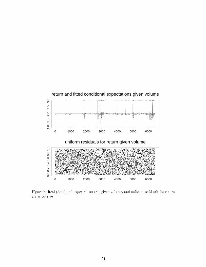
return and fitted conditional expectations given volume
0 1000 2000 3000 4000 5000 6000
1.0
1.5
2.0
2.5
3.0
••••••••
•
••••••••••••••••••••••••••••••••••••••••••••••••••••••••••••••••••
•
•
•••••••••••••••••••••••••••••••••••••••••••••••••••••••••••••••••••••••••••••••••••••••••••••••••••••••••••••••••••••••••••
•
••••••••••••••••••••••••••••••••••••••••••••••••••••••••••••••••••
•
•••••••••••••••••
•
••••••••
•
•••
•
•••••
•
••
•
•••••••••••••••••••••••••••••••••••••••••••••••••
•
••••••••••••••••••••••••••••••••••••••••••••••••••••••••••••••••
•
••
•
••••••••••••••••••••••••••••••••••••••••••••••••••••••••••••••••••••••••••••••••••••••••••••••••••••••••••••••••••••••••••••••••••••••••••••••
•
•••••••••
•
•••
•
•
•
•
•
•
••
••••
•
••
•
•••
•
•
•
••••••••••
•
••••••••••••••••••••••••••••••••••••••••••••••••••••••••••••••••
•
••••••••••
•
•••
•
••••••••••••••••••••••
•
••••••••••••••••••••••••••••••••••••••••••••••••••••••••••••••••••••••••••••••••••••••••••••••••••••••••••••••••
•
•
•
••
•
•
•
•••••••••
•
•
•
••••••••••••••
•
••••••••••••
•
•
•
•
•
•
••
•
•
•
•
•
•
•
••
•
••
•
•
•
•
••
•
••
•
••
•
•
•
••
•
•••
•
••
•
•••
•
••
•
••••••
•
••••
•
••••
•
•••
•
••
•
••
•
•
•
•••••••
•
••
•
••
•
••••
•
••
•
••
•
•
•
•
•
•
•
••
•
•
•
•
•
•
••
•
••
•
••
••
••
•
•
•
•
•
•
•
••
•
•
•
•
••
••
••
•
••
•
•
•
•••
•
•
•
•
•
••••
•
••
•
••••
•
•••••••
•
••
•
•••••
•
•
•
•••
•
•
•
••••
•
•
•
•
•
••••••
•
••••
•
•••••••••••••
••
••
•
••••
•
••••
•
••••••••••••••
•
•••••••
•
••••••••••••••••••••••••••••••
•
•••••••••••••••••••••••••
•
••
•
•••••••••
•
•••••••••••••••••••••••••••••••••••••••••••••••••••••••
•
••••••••••••••••••••••••••••
•
••••••••••••••••••••••••••••
•
•••••••••••
•
•••••••••••••
•
•••••••••••••••••
•
•••
•
•
•
•
••
•
••
•
••••
•
••••
•
•••••••••••••••
•
•••••••
•
•••••••••••••••••••••••••••••••••••••
•
••••
•
•••
•
••••••
•
•••
•
•••••••••
•
••••••••••
•
••••
•
•••
•
••
•
••
•
••
•
••••
•
••••••••••••••••••••••••••
•
••••••••••
•
•••••••••
•
••
•
••••
•
••
•
•
•
•••
•
•••
•
•
•
•••
•
•••••••••••
•
•••
•
•••••••••••••••••••••••••
•
••••••••
•
•••
•
•••••
•
••••
•
••••
•
••••••
•
•••••••••
•
•
•
••••
•
•
•
••
•
•••••••••••••••••••••••••••••••••••••••••
•
•
•
•
••••••
•
••••
•
•
•
•
•
•
•
•
•
••
•
••
•
••
•
•
•
•
•
••
•
••
•
•
•
••
•
•
•
•
•
••
•
••
•
••••
•
•
•
•••
•
•••
•
•••
•
••••••••••••
•
•••••••••
•
••••••••
•
••••••••••
•
••••••••••••••••••••••••••••••••
•
•
•
•••
•
•
•
••••••••••
•
•••••••••••••••
•
••••••••••
•
••
•
••••••••
•
••••••••
•
••••••••••••••
•
•••••••
•
•••••••••••••••••••••••••••••••••
•
•••••••••••••••••••••••••••••••
•
••••••••••••
•
••••••••••••••
•
••
•
••
•
•••
•
••
•
•••
•
••••
•
••••••
•
••
•
•••••
•
•••••
•
••••••••
•
••
•
•••
•
••••••••••••
•
•••
•
•••••••
•
•••••
•
•
•
•
•••••
•
•••••••••
•
••
•
•
•
••
•
•
•
•
•
•
••
•
•••
•
••
•
••••••••••••••
•
•
•••••••••
•
••••
•
••
•
•••
•
••
••
••
•
•
•
•
•
•
•
•
•
•
•
•
•
•
••
•
•
•
•
•
••
•
•
•
•
•
•
•
••
•
•
••
•
••
•
••
•
••
•
•
•
•
•
••••
•
••••
•
•••
•
•••
••
•••
•
••
•
••••••
•
••
•
•••
•
••
•
••
•
••
•
••
uniform residuals for return given volume
0 1000 2000 3000 4000 5000 6000
0.0
0.2
0.4
0.6
0.8
1.0
••
•
•
•••
•
•
•
•
•
•
•
•
••
•
••
••
•
•
•
•
•
•
•
•
•
•
•
•
•
••
•
•
•
•
••
•
•
•
•
•
•
•
•
•
•
••
•
••
•
•
•
•
•
•
••
•
•
•
•
•
•
•
•
•
•
•
•
•
•
•
•
•
•
•
•
•
•
•
•
•
•
••••
•
•
•
•
•
•
•
•
••
•
•
••
•
•
•
•
•
•
•
••
•
•
•
•
••
•
••
•
•
•
••
•
•
••
••
•
•
•
•
•
•
•
•
•
••
•
•
•
•
•
•
•
•
•
••
••
•
•
•
•
•
•••
•
••
•
•
•
••
•
•
•
•
•
•
•
•
•
••
•
•
•
•
•
••
••
•
••
••
•
•
•
•
•
•
•••
•
••
•
•
•
•
•
•
•
•
•
•
••
•
•
•
••
••
•
•
•
•
••
•
•
•
•
••
•
•
•
•
•
•
•
••
•
•
•
•
•
•
•
••
•
•
•
••
•
•
••
•
•
•
••
•
•••
•
•
••
•
•
•
•
•
•••
•
•
•
•
••
•
••
•
•
•
•
•
••
•
•
•
•
•
•
•
•
••
•
•
•
•
•
•
•
•
•
•
•
•
•
•
•
•
•
•
•
•
•
•
•
•
•
•
•
•
•
•
•
•
•
•
•
•
••
•
•
•
•
•
•
••
•
•
•
••
•
•
•
•
•
•
•
•
•
•
•
•
•
•
•
•
•
•
•
•
•
•
•
•
•
•
•
•
•
•
••
•
•
••
•
•••
••
•
•
•
•
•
•
•
•
••
•
•
••
•
•
•
•
•
•
••••••
•
••
•
•
•
•
•
•
•
•
•
••
•
•
•
•
•
•
•
•
•
•
•
•
•
•
•
•
•
•
•
•
•
•
•
•
•
•
•
•
•
•
••
•
•
•
•
••
•
•
•••
•
•
•
•
••
•
•
•
•
•
•
•••
•
•
•
•
•
•
•
•
•
•
•
•
••
••
•
•
•
•
••
•
•
•
•
•
•
•
•
•
•
•
•
•
•
••
•
•
••
•
•
•
•
•
•
•
•
•
•
•
•
•
•
•
••
•
•
•
••
••
•
•
•
•
•
•
••
•
•
••
•
••
•
•
•
•
•
•
•
••
•
•
•
••
•
•
•
•
•
••
•
••
•
•
•
••
•
•
••
•
•
•
•
•
•
•
•
•
•
••
•
•
•
•
•
•
•
•
••
•
••
•
•
•
•
•
•
•
•
•
•
•
•
•
•
•
•
•
•
•
•
•
•
•
•
•
••
•
•
•
••
•
•
•
••
•
•
•
•
••
•
•
•
•
•
•
•
•
•
•
•
•
•
•
••
•
••
•
•
•
•
•
••
•
••
•
•
•
•
•
•
•
•
•
••
•
••
•
•
••
••
•
•
•
•
•
•
•
•
•
•
•
•
•
•
•
••
•
•
•
•
•
•
••••
•
•
•
•
•
•
•
•
•
•
••
•
••
•
•
••
•
•
•
•
•
•
•
•
•
•••
•
•
•
•
•
•
•
•
•
••••
•
•
•
•
•
•
•
••
•
•
•
•
•
•
••
•
•
•
•
•
•
•
•
•
••
•
•
•
•
•
•
•
•
•
•
•
•
•
•
•
•
•
•
•
•
•
••
•
••
•
•
•
•
••
••
•
•
•
•
•
•
•
•
•
•
•
•
••
•
•
•
••
•
•
•
•
•
•
•••
•
••
•
•
•
•
•
•
•
••
•
•
•
•
••
•
•
•
•
•
•
•
•
•
•
•
•
•
•
•
•
•
••
•
•
••
•
•
•
•
••••
•
•
•
•
•
•
•
•
•
••
••
•
•
•
•
•
•
•
•
•
•
•
•
•••
•
•
•
•
••
•
••
••
•
•
•
•
•
•
•
••
•
•
•
•
•
•
•
•
•
••
••
•
•
•
•
•••
•••
•
•
•
•
•
•
•••••
•
•
•
••
•
•
•
••
••
•
•
•
•
•
•
•
•
•
•
•
•
•
•
••••
•
•
•
•
•
•
•
•
•
•
••
•
•
•
••
••
•
•
•
•
•
•
•
•
•
•
•
•
•
•
•
••
•
•
•
•
•
•
•
••
••
•
•••
••••
•
•
•
•
•
•
•
•
•
•
••
•
•
•
•
•
•
•
•
•
••
•
•
•
•
•
•
•
•
•
•
•
•
•
•
•
•
•
•
•
•
•
•
•
•
•••
••
•
•
•
•
•
•
••
•
•
•
••
•••
•
•
•
•
••
•
•
••••
•
•
•
•
•
••
•
•
••
•
•
••
•
•
•
•••
•
•
•
•
•
•
••
•
•
•
•
•
•
•
•
•
•
•
•
•
•
••
•
•
•
••
••
•
•
••
•
•
••
•
•
•
••
•
•
•••
•
•
•
••
••
•••
•
•
•
•
•
•
•
•
•
•••
•
•
•
•
•
•
•
•
•
•
••
•
•
••
•
•
•
•
••
••
••
•
•
•
•
•
••
•
•
•
•
•
•
•
•
••
•
•
••
•
•
•
•
••
••
•
•
•
•
•
•
••
•
•
•
••
••
•
•
•
•
•
•
•
•
•
•
•
••
•
•
••
•
•
•
•
•
•
•
•
••
•
•
•
•
••
•
•
•
•
••
•
••
•
••
••
•
•
•
•
•
•
•
•
•
•
•
••
•
•
•
•
•
•
•
•
•
•
•
•
•
•
•
•
•
••
•
•
•
••
•
•
•
•
•
•
•
•
•
••
•
•
•
••
•
•••
•
••
•
•
•
•
••
••
••
•
••
•
•••
•
•
•
••
•
•
•
•
•
•
•
•
•
•
•
•
•
•
•
•
•
•
•
•
•
••
•
•
•
•
•
•
•
•
•
•
•
•
•
•
•
••
•
•
•
•
•
•
•
••
•
•
•
•
•
•
•
•
•
•
•••
•
•
•
•
•
••
•
•
••
•
•
•
•
•
•
••
••
••••
•
••
••
•
•
•••
•
••
•
••
•
•
•
•
•
•
•
•
•
••
•••
•
•
•
•
•
••
•
•
•
•
••
••
•
••
•
••
•
••
•
•
•
•
•
•
••
••
•
••
•
••
•
•
•
•
•
•
•••
•
•••
•
•
•
••
••
•
•
•
•
•
•
•
•
•
•
•
•
•
•
••
•
••
••
•
••
•
•
••
•
•
•
•
••
•
•
•
•
•
•
••
••
•
•
••
•
••
•
•
•
•
•
•
•
••
•
•
•
•
•
•
•
•
•
•
•
•
•
••
•
•
•
•
••
••
•
•
••
•
•••••
•
•
•
•
•
••••
•
•
•
•
•
•
•
•
•
•
•
•
••
•
•
•
•
•
•
•
•
•
•
•
•
•
•
•
••
•
•
•
•
•
•
•
•
••
•
•
••
•
•
•
•
••
•
•
•
•
•
•
•
•
••
••
••
•
•
•
•
•
•
•
•
•
•
•
•
•••
••
•
•
•
•
•
•
•
•
•
•
•
•
•
•
•
•
••
•
•
•
•
•
•
••
•
••
•
•
•
•
•
•
•
•
•
•
•
•
•
••
•
••
•
•
••
•
•
•
•
•
••
•
••
•
•
••
•
•
•
•
•
••
•
•
•
•
•
•
••
•
•
••
•
•
•
•
•
•
•
•
•
•
•
•
•
••
•
•
•
•
•
••
•
•
•
•
•
••
•
•
•
•
••••
•
•
•
•
•
•
•
••
•
•
•
•
•
•
•
•••
•
•
•
•
•
••
•
••
•
•
•
•
•
•
•
•
••
•
•
•
•
•
••
•
•
•
•
••
•
•
•
•
•
•
•
•
•
••
•
•
•
•
•
•
•
•
••
•
•
•
•
••
•••
•
•
•
•
•
•
•
•
•
•
•
•
•
•
•
••
•
•
•
•
•
•
•
•
•
•
••
••
••
•
•
•••
•
••
•
•
•
••
•
•
•
•
••
•
•
•
•
•
••
•
•
•
•
•
•
•
•
•
•
•
••••
•
•
•
•
••
•
••
•
•
•
•
•
•
•
•
•
•
•
•
•
•••
•
•
•
•
•
••
•
•
•
•
•
•
••
••
•
•
•
•
•
•
•
••
•
•
•
•
•
•
•
•
•
•
•
•
•
•
••
•
•
•
•
•
•
•
•
••
•
•
•
••
•
•
•
••
•
•
•
•
•
•
•
•
•
••
•
•
••
•
•
•
•
•
•
•
•
•
•
•
•
•
•
•
•
•
••
••
•
•
•
•
••
•
•
•
•••
••
••
•
•
•
•
••
•
•••
•
••
••
•
•
•
•
•
•
•
•
•
•
•
•
•
•
•
•
•
•
•
•
•
•
••
•
•
•
•
••
•
••
•
•
•
•
•
•
•
•
•••
•
•
•
•
•
•
••
•
••
•
•
•
••
•
•
•
•
•
•
•
••
•
•
•
•
••
••
•
•
•
•
•
•
•
•
•
•
•
•
•
•
•
•
•
•
•
•
•
••
••
••
•••
•
•
•
•
••
•
•
•
•
•
•
•
•
•
•
•
•
•
•
•
•
•••
•
••
••
••
•
•
••
•
•
•
••
•
•
•
•
•
•
•
•••
•
•
•
•
•
•••
•
•
•
•
•
•
••
•
•
•
••
•
•
•
•
•
•
•••
•
•
•
•
••
•
•
•
•
•
•
••
•
•
•
•
•
•
•
•
•••
•
•
•
•
•
•
••
•
•
•
•
••
•
•
•
•
•
•
•
•
••
•
•
•
•
•
•
•
••
•
••
••
•••
•
••
••
••
••
•
••
•
•
••
••
•
•
•
•
•
•
•
•
•
•
•
•
••
••
•
••
•
•
•
•
••
•
•
•
•
•
•
••
•
•
•
••
•
•••
•
•
•
•
•
•
•
•
•
•
•
•
•
•
••
•
•
•
••
•
•
•
•
••
•
•
••
••
•
•
•
••
•
•
•
•
•
••
•
•
•
•
•
••
•
•
•
•
•
•
•••
••
•
•
•
•
•
•
•
•
•
•
••
•
•
•
•
•
••
•
•
••
••
•
•
•
•
•
••
•
••
•
•
•
•
•
•
•
••
•
•
•
•
•
•
•
•
•
•
•
•
•
•
••
•
••
•
•
•
•
••
•
•
•
•
•
••
•
•
•
••
•
••
•
•
•
•
••
••
•
•
•
•
•
•
•
••
•
•
•
•
•
•
•
•
•
•
••
•
•
•
•
•
•
•
•
•
••
•
•
•
•
•
•
•
•
••
•
•
••
•
••
•
•
•
•
•
•
•
•
•
•
•
••
•
•
•
•••
•
•
•
••••
•
•
•
••
•
•
•
•
•
•
•
•
•
•
•
•
•
•
•
•
•
•
•
•
•
••
•
•
•
•
••
•
•
•
•
•
•
•
•
•
•
•
•
••
•
•
•
•
•
•
•
•
•
•
•••
•
•
••
••
•
••
•
•
•
•
•
•
•
•
••
•
•
•
•
•
•
••
•
•
•
•
•
•
•
•
•
•
••
•
•
•
•
•
••
•
•
•
•
••
•
••••
•
•
•
••
•
••
•
•
••
•
•
•
•
•
•
•
•
••
•
••
•
•
•
•
•
•
•
•
•
•••
•
•
•
•
•
•
•
••
•
•
•
••
•
•
••
•
••
•
•
•
•
•
••
•
••
•
••
•
•••
•••
••
•
•
••
•
•
•
•
•
•
•
•
•
•
•
•
•
•
•
•
•
•
•
•
•
•
•
•
•
•
•
•
•
•
•
•
•
•
••
•
•
••
•
•
•
•
•
•
•
•
•
•
•
•
•
•
•
•
••
•
•
•
•
•
•
•
•
•
•
••
•
•
•
•
•
•
•
•
•
•
•
•
•
••
••
•
•
•
•
•
•
•
•••
•
•
•
•
•
••
•
•
•
•
•
•
••
•
•
•
••
•
••
•
•
•
•
•
••
•
•
•
•
•
•
•
•
•
•
•
•
••
•
•
•
••
•
•
•
•
•
•
•
•••
•
•
•
•
•
••
•
•
•
•
•
••
•
•
•
•
•
•
••
••
•
•
•
•••
•
••
•
•
•
••
•
•
•
•
•
•
•
•
••
•
•
•
••
••
•
•
•
••
•
•
•
•
••
•
•
•
•
•••
•
•
•
•
•
••
••
•
•
•
•
•
•
•
••
•
•
••
•
••
••
•
•
••
•
•
••
•
••
•
•
•
••
•
•
•
•••
•
•
•
•
•
•
•
•
•••
••
•
•
•
•
•
•
•
••
•
•
•
•
•
•
•
•
•
•
•
•
•
•
•
•
•
•
•
•
•
•
•
•
•
•
•
•
•
•
•
•
•
•
•
•
•
•
•
•
••
•
•
•
•
•
•
•
•
•••
•
•
•
•
••
•
••
•
•
••••
•
•
•
•
•
•
•
•
•
•
•
•
•
•••
•
•
••
•
•
•
•
•
••
•
•
•
•
••
•
•
•
•
•
•
•
•
•
•
•
•
•
•
•
••
•
•
•
•
•
•
••
•••
•
•
•
•
•
•
•
•
••
•
•
•
•
••
•
•
•
•
•
••
••
••
•
•
•
•
•
••
•
•
•
•
•
••
•
•
•
•
•
•
•
•
••
•
•
•
•
•
•
•
••
•
•
•
•
•
•
••
••
•
••
•
•
••
•
•
•
•
•••
•
•
•
•
•
•
•
•
••
••
•
•
•
•
•
•
•
•
•
••
•
•
•
••
•
•
•
•
•
•
•
•
•
•
••
•
•
•
•
•
•
•
•
•
•
•
•
•
•
•
•
•
•
•
••
•
•
•
•
•
•••
•
•
•
•
•
•
•
•
•
•
•
•
•
•
•
•
•
•••
•
•
•
•
•
•
•
•
•
•
•
•
•
•
•
•
•
•
•
•
•
•
•
••
•
•
•
•
•
•
•
•
••
•
•
•
•
•
•
•
•
•
•
••
•
•
•
•
•
•
••
•
•
•
•••
•••
•
•
•
•
•
•
••
•
•
•
•
•
•
•
••
•
•
••
•
•
•
•
•
•
•
•
•
•
•
••
•
•
••
•
••
•
•
••
•
•
•
•
•
•
•
•
•
••
•
•
•
•
••
•
••
•
•
•
•
•
•
•
•
•
•
•
•
••
•
•
•
•
•
•
••
•
•
•
•
•
•
•
•
•
•
•
•
•
•
••
•
•
•
•
•
•
•
•
•
•
•
•
•
•
•
•
•
•
•
•
•
••
••
•
•
•
•
•
•
••
•
••
•
•
•
•
•
•
••
••
•
•
•
•
•
••
•
•
•
•
•
•
•
•
•
••
•
•
•
•
•••
•
•
•
•
•
••
•
•
•
•
•
•
•
•
•
•
•
•
•••
•
••
•
•
•
•
•
•
•
•
••
•••
••
••
•
•
•
•
•
••
•
•
•
•
•
••
•
••
•
•
•
•
•
•
•
•
•
•
•
•
•
•
•
•
••
•
•
•
•
•
•
••
•
••
•
•
•
••
•
•
•
•
•
••
••
•
•
•
•
•
•
•
•
•
•
•
•
•
•
•
•
••
•
•
••
•
•
•
•
•
•
••
•
•
•••
•
•
•
•
•
•
•
•
•
•
•
•
••
••
•
•
•
•••
••
•
•
•
•
•
•
•••
••
•••
•
•
•
•
•
•
•
•
•
•
•
•
•
••
•
••
•
•
•
•
•
•
•
•
•
•
•
•
•••
•
•
•
•
••
•
•
•
•
•
•
•
•
•
•
••
•
•
•
•
•
•
•
•
•
•
•
•
•
•
•
•
•
•
•
•
••
••
•
•
•••
•
•
•
•
•
•
•
••
•
•
•
•
•
•
•
•
•
•
•
•
•••
•
•
••
•
•
•••
•
•
•
•
•
•
•
•
•
•
••
•
•
•
•
•
•
•
•
•
•
•
•
••
•
•
••
•
•
•
•
•
•
•
•
•
•
••
•
•
•
•
•
•
•
•
••
•
•
•
•
•
•
•
••
•
•
•
•
•
•
••
•
•
•
•
•
•
••
••
•
•
•
••
•
•
•
•
•
•
••
•
•
•••
•
•
••
••
•
•
••
•••
•
•
•
•
•
•
•
•
••
•
••
•
•
•
•
•
•••
•
•
•
•
•
•
•
•
••
•
•
•
•
•
•
•
•
•
•
•
••
•
•
•
•
•
•
•
•
•
•
•
•
••
••
•
•
•
•
•
•
•
•
•
•
•
•
•
•
•
•
•
•
•
•
•
•
•
••
•
•
•
•
•
•
•
••
•
•
•
•
•
•
••
•
••
•
•
••
••
•
•
•
•
•
•
••
•
•
•
•
•
•
•
•
•
•
•
•
•
•
•
•
•
•
•
•
•
••
•
•
•
••
•
•
•
•
•
••
•
•
•
•
•
•
•
•
•
•
•
•
•
•
•
••
•
•
•
•
•
•
••
•
•
•
•
•••
•
•
•
•
•
•••
•
•
••
•
•
•
•
•••
•
•
•
•
•
•
•
•
••
•
•
•
•
•
••
•
•
•
•
•
•
•••
••
•
•
•
••
••
•
•
•
•
•
•
•
•
•
•
•
•
•
•
••
•
•
•
•
•
•
•
•
•
••••
•
•
•
•
••
•
•
•
•
•
•
••
•
•
•
•
•
•
•
•
•
•
•
•
•••
•
•
•
•
•
••
••
••
•
•
••
••
•
•
•
•
••
•
•
•
•
•
•
•
•
•
•
•
•
•
•
•
•
••
•
••
•
•
•••
•
••••
•
•
•
•
••
•
•
•
•
••
•
•
•
•
•
•
•
••
•
•
••
••
•
•
•
•
•
•
•
•
•
••
•
•
•
•
•
•
•
•
•
•
•
•
•
•
•
•
••
•
••
••
•
•
•
•
•
•
•
•
•
•
•
•
•
•
•
•••
•
•
•
•
•
•
•
•
•
•
•
•
•
•
•
•
•
•••
•
•
•
•
•
•
••
•
•
•
•
•
•
•
•
•
•
•••
•
•
•
•
•
•
•
•
•••
•
•
•
•
•
•
••
•
•
•
••
••
•
•
•
•
•
•••
•
•
•
•
•
•
•
•
•
•
•
•
•
•
•
•
•
•
•
•
•
•
•
•
•
•
•
•
•
•
••
•
•
•••
••
•
•
•
•
•
•
•
•
•
•
•
•
•
•
•
••
•
•
••
•
•
••
•
•
•
•
••
•
•
•
•
•
•
•••
•
•
•
•
••
•
•
•
•
•
•
••
•
•
•
•
•
•
•
•
•
•
•
••
•
••
••
•
•
•
•
•
•
••
•
•
•
•
••
••
•
•
••
•
•
•
•
•
•
•
•
•
•
•
••
•
•••
••
••
•
•
•
•
•
•
•
•
•
•
••
••
••
•
•
•
•
•
•
••
•
•
•
•
••
•
••
•
•
•
••
••
•
•
•
•
••••
•
•
•
•
•
•
•
•
•
•
•
•
••
•
•
•
•
•
••
•
•
•
•
•
•
•
•
•
••
•
•
•
•
•
•
•
•
•
•
•
•
•
•
••
•
•
•
•
•
•
•
•
•
•
•
•
•
•
•
•
•
•••
•
•
•
•
•
•
•
•
•
•
•
•
•
•
••
•
•
•
••
•
•
•
••
•
•
•
•
••
•
••
•
•
•
•
•
•
•
•
•
••
••
•
•••
•
••
•
•
•
••
•
•
•
•
•
•
•
•
•
•
•
•
•
••
•
•
•
•
•
•
••
•
•
•
•
•
••
•
•
•
•
•
•
•
••
•
•
•
•
•
••
•
•
•
•
••
••
•
••
•
•
•
•
•
•
•
•
•
••
•
•
•
•
•
••
•
•
••
•
•
•
•
•
•
•
••
•
•
•••
••
•
••
•
•
•
•
•
•
•
•
••
•
•
•
••••
••
••
•
•
•
•
•
•
•
•
•
•••
••
•
•
•
•
•
•
•
•
•
•
•
•
•
•
•
•
•
•
•
•
•
•
••
••
•
•
•
•
•
•
••
•
•
•
•
•
•
••
•••
•
•
••
•
•
•
•
•
•
•
•
•
•
•
•
•
•
•
•
•
•
•
•
••
•
•
•
•
•
•
••
•
••
•
•
•
•
•
•
•
•
••
•
•
•
•
•
•
••
•
•
••
•
•
•
•
•
•
•
•
•
•
•
•
•
•
•
•
•
•
•
•
••
•
•
••
•••
•
••••
•
•
•
•
•
••
•
••
•
•
••
•
••
•
•
•
••
•
••
•
•
•
•
•
•
•
•
•
•
•
•
•
•
•
•
•
•
•
•
•
•
•
•
•
•
•••
••
•
•
•
••
••
•
•
•
•
•
•
•
•
••
•
•
•
•
••
•
•
•
•
•
•
•
•
•
•
•
•
•••••
•
•
•
•
•
•
••
•
•
•
•
••
•
•
•
•
•
••
•
••
•
•
•
•
•
•
•
•
•
•
••
•
•
••
•
•
•
•
••
•
•
•
•
•
•
•
••
•
••
•
•
•
•
•••
•
•
•
•
••
•
•
••••
••
•
•
••
••
•
•
•
•
•
•
••••
•
•
•
•
•
•
•
•
•
••
••
•
•
•
•
•
•
•
•
•
•
•
•
•
•
•
•
•
•
••
•
•
•
•
•
•
•
•
•
•
•
•
•
•
•
•
•
•
•
•
•
•
•
•
•
•
••
•
•
•
•
•
•
•
••
•
•
••
•
••
•
•
•
••••
••••
•
•
•
•
•
•
•
•
•
•
•
•
••
•
••
•
••
•
•
•
•
•
•
••
•
•••
•
•
•
•
•
•
•
•
•
•
•
•
•
•
•
•
•
•
•
•
•
••
•
••
•
•
•
•
•
•
•
•
•
•
•
•
••
•
•
•
•
•
•
•
•
•
•
•
•
•
•
••
•
•
•
•
•
•
••
•
•
••
•
••
•
•
•
•
•
•
•
•
•
•
••
•
••
•
••
•
•
•
•
•
•
•
•
•
•
•
•
•
••
•
••
•
•
•
•
•
•
••
•
•
•
•
•
•
•
•
•
•
••
••
•
•••
•
•
•
•
••
•
•
•
•
•
•
•
•
•
••
•
•
••
•
••
•
•
•
•
•
•
•
•
•
•
•
•
•
•
•
•
••
•
•
•
•
•
••
•
•
••
•
•
•
•
•
•
•
•
•
•
••
•
•
•
•
•
•
•
•
•
•
••
••
••
•
•
•
•
•
•
•
•
•
••
•
•
•
•
••
•
•
•
•
••
••
••
•
•
•
•
•
•
•
•
•
••
•
•
••
•
•
•
•
•
••
•
•
•
•
•
•
•
••
•
•
•
•
•
•
•
•
••
•
•
•
•
•
••
•
•
•
•
•
•
•
••
•
••••
•
•••
•••
•
•
•
•
•
••
•
••
•
•
•
•
•
••
•
••
•
•
•
•
••
•
•
•
•
•
••
•
••••
•
•
•
•
•
•
•
•
•
•
•
••
•
•
•
•
•
•
•
•
••
•
•
•
•
•
••
•
•
•
•
•
•
••
•
••
•
•
•
•
•••
•
•
•
•
•
•
•
•
••
•
•
•
•
•
•
•
•
•
•
•
•
•
••
•
•
•
•
•
•
•
•
•
•
•
•
•
•
•
•
•
•••
•
•
•
•
•
•
•
•
•
••
•
•
•
•
•
•
•
•
•
•
••
••
•
•
•
•
••
•
•••
•
•
•
•
••
•
•
••
•
••
•
••
•
••
•
••
•
•
•
•
•
•
•
•
•
•
•
•••
•
••
•
•
•
•
•
•
•
•
•
•
•
•
••
•
•
•
•
••
•
•
•
••
••
•
•
•
•
•••
•
•
•
•
•
•
•
••••
••
•
•
•
••••
•
•
•
••
•
•
•
•
•
••
•
•
••
•
•
••
•
•
•
•••
•
•
•
•
••
•
•
•
•••
•
•
•
•
•
•
••
•
•
•
•
•
•
•
•
•
•
•
•
•
•
•
••
•
•
•
•
•
•
•
•
•
•
•
•••••
••
•
•
•
•
•
•
•
•
•
•
•
•
•
••••
•
••
••
•
•
•
•
•
••
••
•
•
•
•••
•
••
••
••
•
••
•
•
•
•
••
•
•
•
•
•
•
•
•
•
•
•
•
••
•
••
•
•
•
•
•
•
•
•
••
•
•
•
•
•
•
•
Figure 7: Real (dots) and expected returns given volume, and uniform residuals for returngiven volume
21

P[V=1|R=1]
0 1000 2000 3000 4000 5000 6000
0.0
0.2
0.4
0.6
0.8
1.0
P[V=1|R=2]
0 1000 2000 3000 4000 5000 6000
0.0
0.2
0.4
0.6
0.8
1.0
P[V=1|R=3]
0 1000 2000 3000 4000 5000 6000
0.0
0.2
0.4
0.6
0.8
1.0
P[V=2|R=1]
0 1000 2000 3000 4000 5000 6000
0.0
0.2
0.4
0.6
0.8
1.0
P[V=2|R=2]
0 1000 2000 3000 4000 5000 6000
0.0
0.2
0.4
0.6
0.8
1.0
P[V=2|R=3]
0 1000 2000 3000 4000 5000 6000
0.0
0.2
0.4
0.6
0.8
1.0
P[V=3|R=1]
0 1000 2000 3000 4000 5000 6000
0.0
0.2
0.4
0.6
0.8
1.0
P[V=3|R=2]
0 1000 2000 3000 4000 5000 6000
0.0
0.2
0.4
0.6
0.8
1.0
P[V=3|R=3]
0 1000 2000 3000 4000 5000 6000
0.0
0.2
0.4
0.6
0.8
1.0
Figure 8: Fitted probabilities for volume given all levels of return
P[V=1|R=1]
0 1000 2000 3000 4000 5000 6000
0.0
0.05
0.10
0.15
P[V=1|R=3]
0 1000 2000 3000 4000 5000 6000
0.0
0.05
0.10
0.15
Figure 9: Fitted probabilities for extremely small volume given the extreme levels of return
22

predicted P[R=1]
6150 6200 6250 6300 6350 6400
0.0
0.2
0.4
0.6
0.8
1.0
predicted P[R=2]
6150 6200 6250 6300 6350 6400
0.0
0.2
0.4
0.6
0.8
1.0
predicted P[R=3]
6150 6200 6250 6300 6350 6400
0.0
0.2
0.4
0.6
0.8
1.0
Figure 10: Predicted probabilities for return
return and predicted return
6150 6200 6250 6300 6350 6400
1.0
1.5
2.0
2.5
3.0
••••••
•
•••••••
•
•••••
•
•••••••••••••••••••••••••••••••••••••••••
•
•
•••••••••••••••••••••••••
•
••••••••
•
••••
•
•••••••••
•
•••••
••••
••
•
•
•
•
•
••
•
•
•
•
•
•
••
•
••••
•
••
•
•
••
••
•
•
••
•
•
•
•
••
•
•
••••
•
•••
•
•••
•
••••
•
••
•
••
•
•••••••••••
•
•••••••••••
•
•••••••
•
•••••••••
••
••••••
•
•••••
•
••••••••••••••••••
•
••••
•
•••••••
•
•••••
•
•••••
•
•••
•
••••••
Figure 11: Real returns (dots) and MAP predictions (line) for returns
23

�2 = 3:80 �3 = �3:85
R1;1 = �0:94 R1;2 = �0:47
R2;1 = 2:72 R2;2 = �0:69
R3;1 = �0:35 R3;2 = �0:07
R4;1 = 0:54 R4;2 = 0:48
R5;1 = �0:33 R5;2 = 0:33
R1;1;2;1 = �0:09 R1;2;2;1 = �0:36 R1;1;2;2 = 0:98 R1;2;2;2 = 0:09
R1;1;3;1 = 1:48 R1;2;3;1 = �0:24 R1;1;3;2 = �0:96 R1;2;3;2 = 0:84
R1;1;4;1 = �0:41 R1;2;4;1 = 0:73 R1;1;4;2 = 0:01 R1;2;4;2 = �0:16
R1;1;5;1 = �0:35 R1;2;5;1 = �0:45 R1;1;5;2 = �0:06 R1;2;5;2 = �0:14
R2;1;3;1 = �0:53 R2;2;3;1 = 0:36 R2;1;3;2 = �0:01 R2;2;3;2 = 0:15
R2;1;4;1 = 0:43 R2;2;4;1 = �0:61 R2;1;4;2 = �0:47 R2;2;4;2 = 0:03
R2;1;5;1 = 1:95 R2;2;5;1 = �0:81 R2;1;5;2 = �2:08 R2;2;5;2 = 0:69
R3;1;4;1 = �2:03 R3;2;4;1 = �0:06 R3;1;4;2 = 1:19 R3;2;4;2 = �0:82
R3;1;5;1 = �0:54 R3;2;5;1 = 1:00 R3;1;5;2 = �0:26 R3;2;5;2 = �0:29
R4;1;5;1 = 2:11 R4;2;5;1 = 0:62 R4;1;5;2 = �0:15 R4;2;5;2 = 0:09
Table 1: MLE estimates for model (3.5)
24
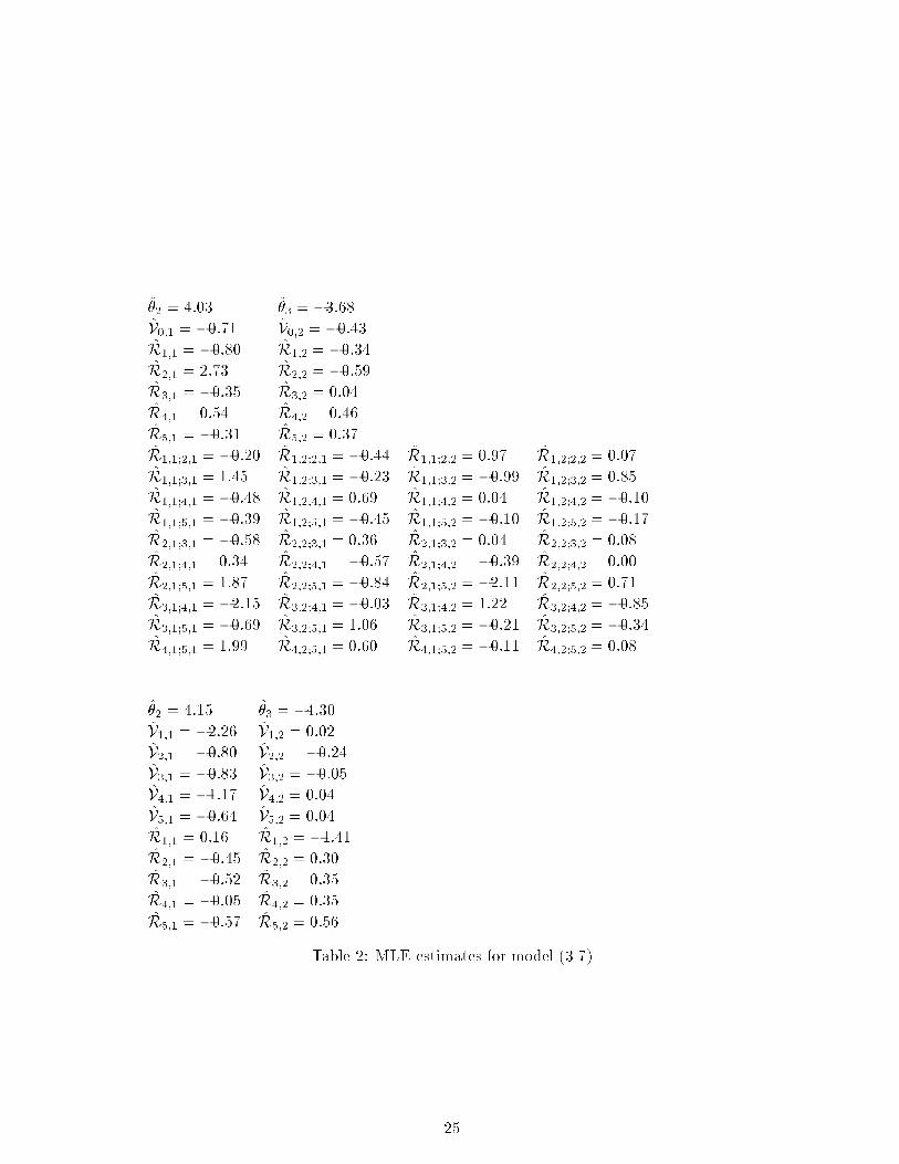
�2 = 4:03 �3 = �3:68
V0;1 = �0:71 V0;2 = �0:43
R1;1 = �0:80 R1;2 = �0:34
R2;1 = 2:73 R2;2 = �0:59
R3;1 = �0:35 R3;2 = 0:04
R4;1 = 0:54 R4;2 = 0:46
R5;1 = �0:31 R5;2 = 0:37
R1;1;2;1 = �0:20 R1;2;2;1 = �0:44 R1;1;2;2 = 0:97 R1;2;2;2 = 0:07
R1;1;3;1 = 1:45 R1;2;3;1 = �0:23 R1;1;3;2 = �0:99 R1;2;3;2 = 0:85
R1;1;4;1 = �0:48 R1;2;4;1 = 0:69 R1;1;4;2 = 0:04 R1;2;4;2 = �0:10
R1;1;5;1 = �0:39 R1;2;5;1 = �0:45 R1;1;5;2 = �0:10 R1;2;5;2 = �0:17
R2;1;3;1 = �0:58 R2;2;3;1 = 0:36 R2;1;3;2 = 0:04 R2;2;3;2 = 0:08
R2;1;4;1 = 0:34 R2;2;4;1 = �0:57 R2;1;4;2 = �0:39 R2;2;4;2 = 0:00
R2;1;5;1 = 1:87 R2;2;5;1 = �0:84 R2;1;5;2 = �2:11 R2;2;5;2 = 0:71
R3;1;4;1 = �2:15 R3;2;4;1 = �0:03 R3;1;4;2 = 1:22 R3;2;4;2 = �0:85
R3;1;5;1 = �0:69 R3;2;5;1 = 1:06 R3;1;5;2 = �0:21 R3;2;5;2 = �0:34
R4;1;5;1 = 1:99 R4;2;5;1 = 0:60 R4;1;5;2 = �0:11 R4;2;5;2 = 0:08
�2 = 4:15 �3 = �4:30
V1;1 = �2:26 V1;2 = 0:02
V2;1 = �0:80 V2;2 = �0:24
V3;1 = �0:83 V3;2 = �0:05
V4;1 = �1:17 V4;2 = 0:04
V5;1 = �0:64 V5;2 = 0:04
R1;1 = 0:16 R1;2 = �1:41
R2;1 = �0:45 R2;2 = 0:30
R3;1 = �0:52 R3;2 = 0:35
R4;1 = �0:05 R4;2 = 0:35
R5;1 = �0:57 R5;2 = 0:56
Table 2: MLE estimates for model (3.7)
25