Empirical Processes in M-Estimationby

Sara van de Geer

Handout at New Directions in General Equilibrium Analysis

Cowles Workshop, Yale University

June 15-20, 2003 Version: June 13, 2003

1

Most of the first part can be found in van de Geer (2000) Empirical Processes in M-Estimation,Cambridge University Press (see also the references therein). The second part also contains morerecent work.

Contents

Part 1Empirical processes and asymptotic normality of M-estimators

1. Introduction

1.1. Law of large numbers for real-valued random variables

1.2. Rd-valued random variables

1.3. Definition Glivenko-Cantelli classes of sets.

2. Which classes are Glivenko-Cantelli classes?

2.1. General Glivenko-Cantelli classes

2.2. Vapnik-Chervonenkis classes

3. Convergence of means to their expectations

3.1. Uniform law of large numbers for classes of functions

3.2. VC classes of functions

3.3. Exercises

4. Uniform central limit theorems

4.1. Real-valued random variables

4.2. Rd-valued random variables

4.3. Donsker’s theorem

4.4. Donsker classes

5. M-estimators

5.1. What is an M-estimator?

5.2. Consistency and uniform laws of large numbers

5.3. Asymptotic normality of M-estimators

2

5.4. Conditions a, b and c for asymptotic normality

5.5. Asymptotics for the median

5.6. Conditions A, B and C for asymptotic normality

5.7. Exercise

Part 2Empirical processes and regularization of M-estimators

1. A classical approach

2. The sequence space model

3. Sparse signals

4. A concentration inequality

5. Hard and soft thresholding

6. The oracle

7. Discretization

8. General penalties

9. Application to the classical penalty

10. Robust regression

11. Density estimation

12. Classification

13. Some references for Part 2

3

Part 1Empirical processes and asymptotic normality of M-estimators

1. Introduction. Let X1, . . . , Xn, . . . be i.i.d. copies of a random variable X with values in X andwith distribution P .

1.1. Law of large numbers for real-valued random variables. Consider the case X = R.Suppose the mean

µ = EX

exists. Define the average

Xn =1n

n∑i=1

Xi, n ≥ 1.

Then, by the law of large numbers, as n→∞,

Xn → µ, a.s.

Now, letF (t) = P (X ≤ t), t ∈ R,

be the theoretical distribution function, and

Fn(t) =1n

#{Xi ≤ t, 1 ≤ i ≤ n}, t ∈ R,

be the empirical distribution function. Then by the law of large numbers, as n→∞,

Fn(t) → F (t), a.s. for all t.

The Glivenko-Cantelli Theorem says that

supt|Fn(t)− F (t)| → 0, a.s.

This is a uniform law of large numbers.

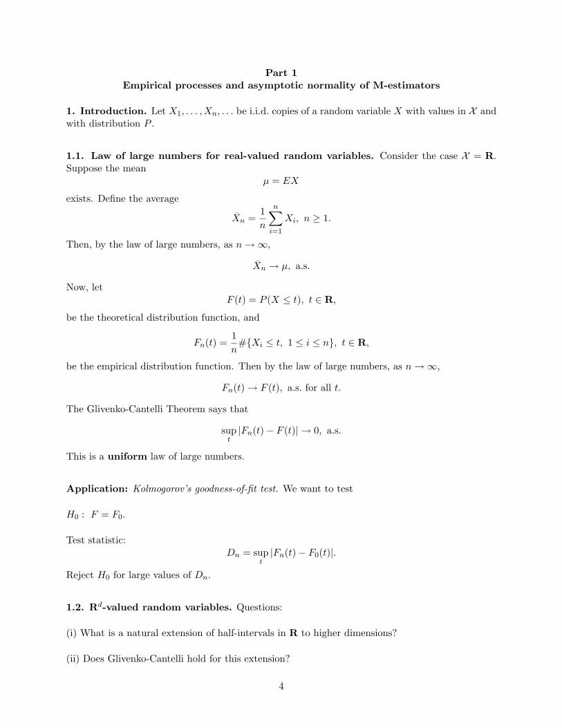
Application: Kolmogorov’s goodness-of-fit test. We want to test

H0 : F = F0.

Test statistic:Dn = sup

t|Fn(t)− F0(t)|.

Reject H0 for large values of Dn.

1.2. Rd-valued random variables. Questions:

(i) What is a natural extension of half-intervals in R to higher dimensions?

(ii) Does Glivenko-Cantelli hold for this extension?

4

1.3. Definition Glivenko-Cantelli classes of sets. Let for any (measurable1) A ⊂ X ,

Pn(A) =1n

#{Xi ∈ A, 1 ≤ i ≤ n}.

We call Pn the empirical measure (based on X1, . . . , Xn).

Let D be a collection of subsets of X .

Definition 1.3.1. The collection D is called a Glivenko-Cantelli (GC) class if

supD∈D

|Pn(D)− P (D)| → 0, a.s.

Example. Let X = R. The class of half-intervals

D = {l(−∞,t] : t ∈ R}

is GC. But when e.g. P = uniform distribution on [0, 1] (i.e., F (t) = t, 0 ≤ t ≤ 1), the class

B = {all (Borel) subsets of [0, 1]}

is not GC.

2. Which classes are Glivenko-Cantelli classes?

2.1. General GC classes. Let D be a collection of subsets of X , and let {ξ1, . . . , ξn} be n pointsin X .

Definition 2.1.1. We write

4D(ξ1, . . . , ξn) = card({D ∩ {ξ1, . . . , ξn} : D ∈ D}

= the number of subsets of {ξ1, . . . , ξn} that D can distinguish.

That is, count the number of sets in D, when two sets D1 and D2 are considered as equal ifD14D2 ∩ {ξ1, . . . , ξn} = ∅. Here

D14D2 = (D1 ∩Dc2) ∪ (Dc

1 ∩D2)1We will skip measurability issues, and most of the time do not mention explicitly the requirement of measurability

of certain sets or functions. This means that everything has to be understood modulo measurability.

5

is the symmetric difference between D1 and D2.

Remark. For our purposes, we will not need to calculate 4D(ξ1, . . . , ξn) exactly, but only a goodenough upper bound.

Example. Let X = R andD = {l(−∞,t] : t ∈ R}.

Then for all {ξ1, . . . , ξn} ⊂ R4D(ξ1, . . . , ξn) ≤ n+ 1.

Example. Let D be the collection of all finite subsets of X . Then, if the points ξ1, . . . , ξn aredistinct,

4D(ξ1, . . . , ξn) = 2n.

Notation. The simultaneous distribution of (X1, . . . , Xn, . . .) is denoted by

P = P × . . .× P × . . . .

Theorem 2.1.2. (Vapnik and Chervonenkis (1971)). We have

supD∈D

|Pn(D)− P (D)| → 0 a.s.

if and only if1n

log ∆D(X1, . . . , Xn) →P 0.

tu

2.2. Vapnik-Chervonenkis classes.

Definition 2.2.1. Let

mD(n) = sup{4D(ξ1, . . . , ξn) : ξ1, . . . , ξn ∈ X}.

We say that D is a Vapnik-Chervonenkis (VC) class if for certain constants c and r, and for alln,

mD(n) ≤ cnr,

i.e., if mD(n) does not grow faster than a polynomial in n.

Important conclusion: For sets, VC ⇒ GC.

Examples.

6

a) X = R, D = {l(−∞,t] : t ∈ R}. Since mD(n) ≤ n+ 1, D is VC.

b) X = Rd, D = {l(−∞,t] : t ∈ Rd}. Since mD(n) ≤ (n+ 1)d, D is VC.

c) X = Rd, D = {{x : θTx > t},(θt

)∈ Rd+1}. Since mD(n) ≤ 2d

(nd

), D is VC.

The VC property is closed under measure theoretic operations:

Lemma 2.2.2. Let D, D1 and D2 be VC. Then the following classes are also VC:

(i) Dc = {Dc : D ∈ D},

(ii) D1 ∩ D2 = {D1 ∩D2 : D1 ∈ D1, D2 ∈ D2},

(iii) D1 ∪ D2 = {D1 ∩D2 : D1 ∈ D1, D2 ∈ D2}. tu

Examples.

- the class of intersections of two halfspaces,

- all ellipsoids,

- all half-ellipsoids,

- in R, the class {{x : θ1x+ . . .+ θrxr ≤ t} :

(θt

)∈ Rr+1}.

There are classes that are GC, but not VC.

Example. Let X = [0, 1]2, and let D be the collection of all convex subsets of X . Then D is notVC, but when P is uniform, D is GC.

Finally, we will not deny you the following definition and a very nice lemma.

Definition 2.2.3. The VC dimension of D is

V (D) = inf{n : mD(n) < 2n}.

Lemma 2.2.4. We have that D is VC if and only if V (D) <∞. tu

3. Convergence of means to expectations.

7

Notation. For a function g : X → R, we write∫gdP = Eg(X),

and ∫gdPn =

1n

n∑i=1

g(Xi).

3.1. Uniform law of large numbers for classes of functions. Let G be a collection ofreal-valued functions on X .

Definition 3.1.1. The class G is called a Glivenko-Cantelli (GC) class if

supg∈G

|∫gdPn −

∫gdP | → 0, a.s.

Example. G = {lD : D ∈ D} is GC if D is GC.

3.2. VC classes of functions.

Definition 3.2.1. The subgraph of a function g : X → R is

subgraph(g) = {(x, t) ∈ X ×R : g(x) ≥ t}.

A collection of functions G is called a VC class if the subgraphs {subgraph(g) : g ∈ G} form a VCclass.

Examples (X = Rd).

a) G = {g(x) = θ0 + θ1x1 + . . .+ θdxd : θ ∈ Rd+1},

b) G = {g(x) = |θ0 + θ1x1 + . . .+ θdxd| : θ ∈ Rd+1} .

c) d = 1, G =

g(x) ={a+ bx if x ≤ cd+ ex if x > c

,

abcde

∈ R5

,

d) d = 1, G = {g(x) = eθx : θ ∈ R}.

Definition 3.2.2. The envelope G of a collection of functions G is defined by

G(x) = supg∈G

|g(x)|, x ∈ X .

8

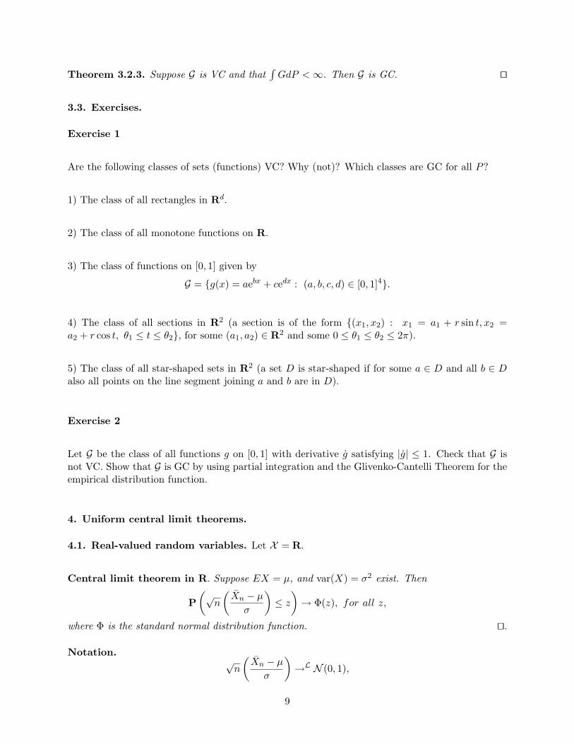
Theorem 3.2.3. Suppose G is VC and that∫GdP <∞. Then G is GC. tu

3.3. Exercises.

Exercise 1

Are the following classes of sets (functions) VC? Why (not)? Which classes are GC for all P?

1) The class of all rectangles in Rd.

2) The class of all monotone functions on R.

3) The class of functions on [0, 1] given by

G = {g(x) = aebx + cedx : (a, b, c, d) ∈ [0, 1]4}.

4) The class of all sections in R2 (a section is of the form {(x1, x2) : x1 = a1 + r sin t, x2 =a2 + r cos t, θ1 ≤ t ≤ θ2}, for some (a1, a2) ∈ R2 and some 0 ≤ θ1 ≤ θ2 ≤ 2π).

5) The class of all star-shaped sets in R2 (a set D is star-shaped if for some a ∈ D and all b ∈ Dalso all points on the line segment joining a and b are in D).

Exercise 2

Let G be the class of all functions g on [0, 1] with derivative g satisfying |g| ≤ 1. Check that G isnot VC. Show that G is GC by using partial integration and the Glivenko-Cantelli Theorem for theempirical distribution function.

4. Uniform central limit theorems.

4.1. Real-valued random variables. Let X = R.

Central limit theorem in R. Suppose EX = µ, and var(X) = σ2 exist. Then

P(√

n

(Xn − µ

σ

)≤ z

)→ Φ(z), for all z,

where Φ is the standard normal distribution function. tu.

Notation.√n

(Xn − µ

σ

)→L N (0, 1),

9

or √n(Xn − µ) →L N (0, σ2).

4.2. Rd-valued random variables. Let X1, X2, . . . be i.i.d. Rd-valued random variables, copiesof X (X ∈ X = Rd), with expectation µ = EX, and covariance matrix Σ = EXXT − µµT .

Central limit theorem in Rd. We have√n(Xn − µ) →L N (0,Σ),

i.e. √n[aT (Xn − µ)

]→L N (0, aTΣa), for all a ∈ Rd.

tu.

4.3. Donsker’s Theorem. Let X = R. Recall the definition of the distribution function F andthe empirical distribution function Fn:

F (t) = P (X1 ≤ t), t ∈ R,

Fn(t) =1n

#{Xi ≤ t, 1 ≤ i ≤ n}, t ∈ R.

By the central limit theorem in R (Section 4.1), for all t√n(Fn(t)− F (t)) →L N (0, F (t)(1− F (t))) .

Also, by the central limit theorem in R2 (Section 4.2), for all s < t,

√n

(Fn(s)− F (s)Fn(t)− F (t)

)→L N (0,Σ(s, t)),

where

Σ(s, t) =(F (s)(1− F (s)) F (s)(1− F (t))F (s)(1− F (t)) F (t)(1− F (t))

).

We are now going to consider the stochastic process Wn = {Wn(t) : t ∈ R}. The process Wn iscalled the (classical) empirical process.

Definition 4.3.1. Let K0 be the collection of bounded functions on [0, 1]. The stochastic processB(·) ∈ K0, is called the standard Brownian bridge if

- B(0) = B(1) = 0,

- for all r ≥ 1 and all t1, . . . , tr ∈ (0, 1), the vector

B(t1)...

B(tr)

is multivariate normal with mean

zero,

10

- for all s ≤ t, cov(B(s), B(t)) = s(1− t).

- the sample paths of B are a.s. continuous.

Donsker’s theorem. Consider Wn and WF = B ◦ F as elements of the space K of boundedfunctions on R. We have

Wn →L WF ,

that is,Ef(Wn) → Ef(WF ),

for all continuous and bounded functions f . tu

Reflection. Suppose F is continuous. Then, since B is almost surely continuous, also WF = B ◦Fis almost surely continuous. So Wn must be approximately continuous as well in some sense.Indeed, we have for any t and any sequence tn converging to t,

|Wn(tn)−Wn(t)| →P 0.

This is called asymptotic continuity.

4.4. Donsker classes. Let X1, . . . , Xn, . . . be i.i.d. copies of a random variable X, with values inthe space X , and with distribution P . Consider a class G of functions g : X → R. The (theoretical)mean of a function g is ∫

gdP = Eg(X),

and the (empirical) average (based on the n observations X1, . . . , Xn) is∫gdPn =

1n

n∑i=1

g(Xi).

Here Pn is the empirical distribution (based on X1, . . . , Xn).

Definition 4.4.1. The empirical process indexed by G is

νn(g) =√n

∫gd(Pn − P ), g ∈ G.

Let us recall the central limit theorem for g fixed. Denote the variance of g(X) by

σ2(g) = var(g(X)) = Eg2(X)− (Eg(X))2.

If σ2(g) <∞, we haveνn(g) →L N (0, σ2(g)).

11

The central limit theorem also holds for finitely many g simultaneously. Let gk and gl be twofunctions and denote the covariance between gk(X) and gl(X) by

σ(gk, gl) = cov(gk(X), gl(X)) = Egk(X)gl(X)− Egk(X)Egl(X).

Then, whenever σ2(gk) <∞ for k = 1, . . . , r, νn(g1)...

νn(gr)

→L N (0,Σg1,...,gr),

where Σg1,...,gr is the variance-covariance matrix

(∗) Σg1,...,gr =

σ2(g1) . . . σ(g1, gr)...

. . ....

σ(g1, gr) . . . σ2(gr)

.

Definition 4.4.2. Let ν be a Gaussian process indexed by G. Assume that for each r ∈ N and foreach finite collection {g1, . . . , gr} ⊂ G, the r-dimensional vector ν(g1)

...ν(gr)

has a N (0,Σg1,...,gr)-distribution, with Σg1,...,gr defined in (*). We then call ν the P -Brownianbridge indexed by G.

Definition 4.4.3. Consider νn and ν as bounded functions on G. We call G a P -Donsker class if

νn →L ν,

that is, if for all continuous and bounded functions f , we have

Ef(νn) → Ef(ν).

Definition 4.4.4. The process νn on G is called asymptotically continuous if for all g0 ∈ G,and all (possibly random) sequences {gn} ⊂ G with σ(gn − g0) →P 0, we have

|νn(gn)− νn(g0)| →P 0.

We will use the notation‖g‖2 =

∫g2dP,

i.e., ‖ · ‖ is the L2(P )-norm.

Remark. Note that σ(g) ≤ ‖g‖.

12

Definition 4.4.5. The class G ⊂ L2(P ) is called totally bounded if for all δ > 0 the number ofballs with radius δ necessary to cover G is finite.

Theorem 4.4.6. Suppose that G is totally bounded. Then G is a P -Donsker class if and only if νn(as process on G) is asymptotically continuous.

tu

Theorem 4.4.7. Suppose that G is a VC-graph class with envelope

G = supg∈G

|g|

satisfying∫G2dP <∞. Then G is P -Donsker.

tu

Remark. Thus, a VC class G with square integrable envelope G is asymptotically continuous. Inparticular, suppose that such a class G is parametrized by θ in some parameter space Θ ⊂ Rr (say),i.e. G = {gθ : θ ∈ Θ}. Let zn(θ) = νn(gθ). Question: do we have that for a (random) sequence θnwith θn → θ0 (in probability), also

|zn(θn)− zn(θ0)| →P 0 ?

Indeed, if σ(gθ−gθ0) converges to zero as θ converges to θ0, the answer is yes. And so ‖gθ−gθ0‖ → 0(mean square convergence) suffices for a yes answer.

5. M-estimators.

5.1. What is an M-estimator? Let X1, . . . , Xn, . . . be i.i.d. copies of a random variable X withvalues in X and with distribution P .

Let Θ be a parameter space (a subset of some metric space) and let

γθ : X → R,

be some loss function. We estimate the unknown parameter

θ0 = arg minθ∈Θ

∫γθdP,

by the M-estimator

θn = arg minθ∈Θ

∫γθdPn.

Here, we assume that θ0 exists and is unique and that θn exists.

Examples.

13

(i) Location estimators. X = R, Θ = R, and

(i.a) γθ(x) = (x− θ)2 (estimating the mean),

(i.b) γθ(x) = |x− θ| (estimating the median).

(ii) Maximum likelihood. Let {pθ : θ ∈ Θ} be a family of densities w.r.t. a σ-finite dominatingmeasure µ, and

ρθ = − log pθ.

If dP/dµ = pθ0 , θ0 ∈ Θ, then indeed θ0 is a minimizer of∫ρθdP , θ ∈ Θ.

(ii.a) Poisson distribution:

pθ(x) = eθθx

x!, x ∈ {1, 2, . . .}, θ > 0.

(ii.b) Logistic distribution:

pθ(x) =eθ−x

(1 + eθ−x)2, x ∈ R, θ ∈ R.

5.2. Consistency and the law of large numbers. Define for θ ∈ Θ,

Γ(θ) =∫γθdP,

andΓn(θ) =

∫γθdPn.

We first present an easy proposition with a too stringent condition (•).

Proposition 5.2.1. Suppose that θ 7→ Γ(θ) is continuous. Assume moreover that

(•) supθ∈Θ

|Γn(θ)− Γ(θ)| → 0, a.s.,

i.e., that {γθ : θ ∈ Θ} is a GC class. Then θn → θ0 a.s. tu

The assumption (•) is hardly ever met, because it is close to requiring compactness of Θ. Wegive a lemma, which replaces (•) by a convexity assumption. This works out well when Θ is finitedimensional.

Lemma 5.2.2. Suppose that Θ is a convex subset of Rr, and that θ 7→ γθ, θ ∈ Θ is convex. Thenθn → θ0, a.s. tu

14

5.3. Asymptotic normality of M-estimators. In this section, we assume that we alreadyshowed that θn is consistent, and that θ0 is an interior point of Θ ⊂ Rr.

Definition 5.3.1. The (sequence of) estimator(s) θn of θ0 is called asymptotically linear if wemay write

√n(θn − θ0) =

√n

∫ldPn + oP(1),

where

l =

l1...lr

: X → Rr,

satisfies∫ldP = 0 and

∫l2kdP < ∞, k = 1, . . . , r. The function l is then called the influence

function. For the case r = 1, we call σ2 =∫l2dP the asymptotic variance.

Definition 5.3.2. Let θn,1 and θn,2 be two asymptotically linear estimators of θ0, with asymptoticvariances σ2

1 and σ22 respectively. Then

e1,2 =σ2

2

σ21

is called the asymptotic relative efficiency (of θn,1 as compared to θn,2).

5.4. Conditions a, b and c for asymptotic normality. We start with three conditions a, band c, which are easier to check but more stringent. We later relax them to conditions A, B and C.

Condition a. There exists an ε > 0 such that θ 7→ γθ is differentiable for all |θ − θ0| < ε and allx, with derivative

ψθ(x) =∂

∂θγθ(x), x ∈ X .

Condition b. We have as θ → θ0,∫(ψθ − ψθ0)dP = V (θ − θ0) + o(1)|θ − θ0|,

where V is a positive definite matrix.

Condition c. There exists an ε > 0 such that the class

{ψθ : |θ − θ0| < ε}

has envelope Ψ ∈ L2(P ) and is Donsker. Moreover,

limθ→θ0

‖ψθ − ψθ0‖ = 0.

15

Lemma 5.4.1. Suppose conditions a, b and c. Then θn is asymptotically linear with influencefunction

l = −V −1ψθ0 ,

so √n(θn − θ0) →L N (0, V −1JV −1),

whereJ =

∫ψθ0ψ

Tθ0dP.

tu

Example: Huber estimator. Let X = R, Θ = R. The Huber estimator corresponds to the lossfunction

γθ(x) = γ(x− θ),

withγ(x) = x2l{|x− θ| ≤ k}+ (2k|x| − k2)l{|x| > k}, x ∈ R.

Here, 0 < k <∞ is some fixed constant, chosen by the statistician. We will now verify a, b and c.

a)

ψθ(x) =

{ 2k if x− θ ≤= k−2(x− θ) if |x− θ| ≤ k−2k if x− θ ≥ k

.

b) We haved

dθ

∫ψθdP = 2(F (k + θ)− F (−k + θ)),

where F (t) = P (X ≤ t), t ∈ R is the distribution function. So

V = 2(F (k + θ0)− F (−k + θ0)).

c) Clearly ψθ : θ ∈ R is a VC class, with envelope Ψ ≤ 2k.

So the Huber estimator θn is asymptotically linear, with influence function

l(x) =

− kF (k+θ0)−F (−k+θ0) if x− θ0 ≤ −k

x−θ0F (k+θ0)−F (−k+θ0) if |x− θ0| ≤ k

kF (k+θ0)−F (−k+θ0) if x− θ0 > k

.

The asymptotic variance is

σ2 =k2F (−k + θ0) =

∫ k+θ0−k+θ0(x− θ0)2dF (x) + k2(1− F (k + θ0))

(F (k + θ0)− F (k + θ0))2.

5.5. Asymptotics for the median. The median (see Example (i.b)) can be regarded as thelimiting case of a Huber estimator, with k ↓ 0. However, the loss function γθ(x) = |x − θ| is not

16

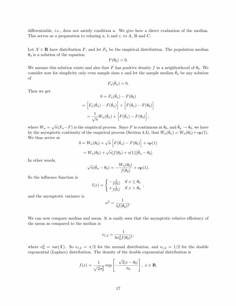
differentiable, i.e., does not satisfy condition a. We give here a direct evaluation of the median.This serves as a preparation to relaxing a, b and c, to A, B and C.

Let X ∈ R have distribution F , and let Fn be the empirical distribution. The population medianθ0 is a solution of the equation

F (θ0) = 0.

We assume this solution exists and also that F has positive density f in a neighborhood of θ0. Weconsider now for simplicity only even sample sizes n and let the sample median θn be any solutionof

Fn(θn) = 0.

Then we get0 = Fn(θn)− F (θ0)

=[Fn(θn)− F (θn)

]+[F (θn)− F (θ0)

]=

1√nWn(θn) +

[F (θn)− F (θ0)

],

where Wn =√n(Fn−F ) is the empirical process. Since F is continuous at θ0, and θn → θ0, we have

by the asymptotic continuity of the empirical process (Section 4.3), that Wn(θn) = Wn(θ0)+oP(1).We thus arrive at

0 = Wn(θ0) +√n[F (θn)− F (θ0)

]+ oP(1)

= Wn(θ0) +√n[f(θ0) + o(1)][θn − θ0].

In other words,√n(θn − θ0) = −Wn(θ0)

f(θ0)+ oP(1).

So the influence function is

l(x) =

{− 1f(θ0) if x ≤ θ0

+ 1f(θ0) if x > θ0

,

and the asymptotic variance is

σ2 =1

4f(θ0)2.

We can now compare median and mean. It is easily seen that the asymptotic relative efficiency ofthe mean as compared to the median is

e1,2 =1

4σ20f(θ0)2

,

where σ20 = var(X). So e1,2 = π/2 for the normal distribution, and e1,2 = 1/2 for the double

exponential (Laplace) distribution. The density of the double exponential distribution is

f(x) =1√2σ2

0

exp

[−√

2|x− θ0|σ0

], x ∈ R.

17

Exercise. Suppose X has the logistic distribution with location parameter θ (see Example (ii.b)).Show that the maximum likelihood estimator has asymptotic variance equal to 3, and the medianhas asymptotic variance equal to 4. Hence, the asymptotic relative efficiency of the maximumlikelihood estimator as compared to the median is 4/3.

5.6. Conditions A, B and C for asymptotic normality. In this section, we again assumethat we already showed that θn is consistent, and that θ0 is an interior point of Θ ⊂ Rr. We arenow going to relax the condition of differentiability of γθ.

Condition A. (Differentiability in quadratic mean.) There exists a function ψ0 : X → Rr, withcomponents in L2(P ), such that

limθ→θ0

∥∥γθ − γθ0 − (θ − θ0)Tψ0

∥∥|θ − θ0|

= 0.

Condition B. We have as θ → θ0,

Γ(θ)− Γ(θ0) =12(θ − θ0)TV (θ − θ0) + o(1)|θ − θ0|2,

with V a positive definite matrix.

Condition C. Define for θ 6= θ0,

gθ =(γθ − γθ0)|θ − θ0|

.

Suppose that for some ε > 0, the class {gθ : 0 < |θ − θ0| < ε} has envelope G ∈ L2(P ) and that itis a Donsker class.

Lemma 5.6.1. Suppose conditions A, B and C are met. Then θn has influence function

l = −V −1ψ0,

and so √n(θn − θ0) →L N (0, V −1JV −1),

where J =∫ψ0ψ

T0 dP . tu

5.7. Exercise. Let (Xi, Yi), i = 1, . . . , n, . . . be i.i.d. copies of (X,Y ), where X ∈ Rd and Y ∈ R.Suppose that the conditional distribution of Y givenX = x has medianm(x) = α0+α1x1+. . . αdxd,with

α =

α0...αd

∈ Rd+1.

Assume moreover that given X = x, the random variable Y −m(x) has a density f not dependingon x, with f positive in a neighborhood of zero. Suppose moreover that

Σ = E

(1 XX XXT

)18

exists. Let

αn = arg mina∈Rd+1

1n

n∑i=1

|Yi − a0 − a1Xi,1 − . . .− adXi,d| ,

be the least absolute deviations (LAD) estimator. Show that

√n(αn − α) →L N

(0,

14f2(0)

Σ−1

),

by verifying conditions A, B and C.

19

Part 2Empirical processes and regularization of M-estimators

1. A classical approach.

Yi = f0(xi) + εi, i = 1, . . . , n.

• ε1, . . . , εn independent N (0, σ2).

• xi = i/n, i = 1, . . . , n.

• f0 : [0, 1] → R unknown function.

• Yi ∈ R observations.

“Classical” estimator:

fn = arg minf

{1n

n∑i=1

|Yi − f(xi)|2 + λ2n

∫ 1

0|f ′(x)|2dx

}.

Continuous version:

f = arg minf

{∫ 1

0|y(x)− f(x)|2dx+ λ2

∫ 1

0|f ′(x)|2dx

}.

Lemma 1.1. Solution:

f(x) =C

λcosh(

x

λ) +

1λ

∫ x

0y(u) sinh(

u− x

λ)du,

where

C = Y (1)−{

1λ

∫ 1

0Y (u) sinh(

1− u

λ)du}/ sinh(

1λ

),

withY (x) =

∫ x

0y(u)du.

tu

Choice of regularization parameter λ? E.g.,

fn = arg minf

minλ

{1n

n∑i=1

|Yi − f(xi)|2 +(λ2

∫ 1

0|f ′(x)|2dx+

c

nλ

)}.

20

Here is the a MATLAB script for calculating the solution given in Lemma 1.1:

function smooth = smooth1(data,lambda)% SMOOTH1 requires an input vector DATA and a regularization parameter LAMBDA% SMOOTH1 calculates the smoothed version of the input vector DATA% it uses a penalty on the squared L2 norm of the derivative of the function% n=the number of observations% the output FIT is the squared (normalized) L2 norm of the difference between% DATA and fitted function

lambdasigma=1/lambda;

n=size(data)*[1,1]'-1

dt = 1/(n-1);x = [0:dt:1];

plot(x, data, 'r');hold on;

size_x = size(x);temp = zeros(size_x(2), 1);temp2 = 0;

DATA = 0;for j = 1:size_x(2) DATA = DATA + data(j) * dt; end;

C = 0;for j = 1:size_x(2) C = C + data(j) * (cosh(sigma * (-1 + j * dt))); end;C = (-DATA * (0) + C * dt) / sinh(sigma);

for i = 1:size_x(2) temp2 = 0; for j = 1:i temp2 = temp2 + data(j) * sinh(sigma * (j - i) * dt); end; temp(i) = C * sigma * cosh(sigma * i * dt) + sigma * temp2 * dt;end;

plot(x, temp, 'g');fit=(data-temp')*(data'-temp)/n

hold off

21

0 10 20 30 40 50 60 70 80 90 100-0.16

-0.14

-0.12

-0.1

-0.08

-0.06

-0.04

-0.02

0

True f

0 10 20 30 40 50 60 70 80 90 100-0.18

-0.16

-0.14

-0.12

-0.1

-0.08

-0.06

-0.04

-0.02

0

0.02

Noise added, noise level = 0.01

22

0 0.1 0.2 0.3 0.4 0.5 0.6 0.7 0.8 0.9 1-0.18

-0.16

-0.14

-0.12

-0.1

-0.08

-0.06

-0.04

-0.02

0

0.02

Denoised, lambda=0.2Fit=9.0531e-04

0 0.1 0.2 0.3 0.4 0.5 0.6 0.7 0.8 0.9 1-0.18

-0.16

-0.14

-0.12

-0.1

-0.08

-0.06

-0.04

-0.02

0

0.02

Denoised, lambda=0.1Fit=3.4322e-04

23

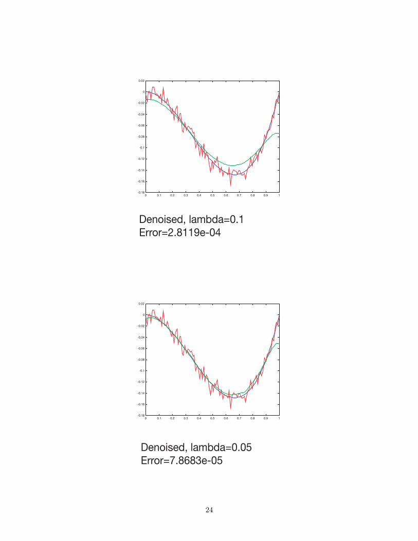
0 0.1 0.2 0.3 0.4 0.5 0.6 0.7 0.8 0.9 1-0.18

-0.16

-0.14

-0.12

-0.1

-0.08

-0.06

-0.04

-0.02

0

0.02

Denoised, lambda=0.1Error=2.8119e-04

0 0.1 0.2 0.3 0.4 0.5 0.6 0.7 0.8 0.9 1-0.18

-0.16

-0.14

-0.12

-0.1

-0.08

-0.06

-0.04

-0.02

0

0.02

Denoised, lambda=0.05Error=7.8683e-05

24

2. The sequence space model.

Yi = f0(xi) + εi, i = 1, . . . , n.

with ε1, . . . , εn independent N (0, σ2), and xi ∈ X , Yi ∈ R, i = 1, . . . , n.

Let

Qn =1n

n∑i=1

δXi .

Let ψ1, . . . , ψn be an orthonormal basis of L2(Qn) (ψj : X → R, j = 1, . . . , n). Define

Yj =1n

n∑i=1

Yiψj(xi), j = 1, . . . , n,

εj =1n

n∑i=1

εiψj(xi), j = 1, . . . , n,

θj =1n

n∑i=1

f0(xi)ψj(xi), j = 1, . . . , n.

ThenYj = θj + εj , j = 1, . . . , n,

with ε1, . . . , εn independent N (0, σ2

n ).

25

• Fourier

• Wavelets

• Trigonometric

• Polynomial

• ....

3. Sparse signals.

Yj = θj + εj , j = 1, . . . , n,

with ε1, . . . , εn independent N (0, σ2

n ),

Define

‖ϑ‖2n =

n∑j=1

|ϑj |2, ϑ ∈ Rn.

Definition 3.1. Let 0 ≤ r < 2. The signal θ is called r-sparse if

n∑j=1

|θj |r ≤ 1.

Lemma 3.2. Suppose θ is r-sparse. Then

#{|θj | > λ} ≤ λ−r.

tu

Lemma 3.3. Let

θ∗j ={θj if |θj | > λ0 if |θj | ≤ λ

.

If θ is r-sparse we have‖θ∗ − θ‖2

n ≤ λ2−r.

tu

26

A sparse signal......

27

4. A concentration inequality.

Lemma 4.1. Let ε1, . . . , εn be independent N (0, 1). Then

max1≤j≤n

|εj | ≤√

6 log n, a.s.,

for n sufficiently large.

Proof. We have for all a > 0, and γ > 0, by Chebyshev’s inequality

P (εj > a) ≤ E exp[γεj ]exp[γa]

= exp[12γ2 − γa].

Take γ = a to arrive at

P (εj > a) ≤ exp[−12a2].

So

P(

max1≤j≤n

|εj | > a

)≤ 2n exp[−1

2a2].

Take a =√

6 log n to get

P(

max1≤j≤n

|εj | >√

6 log n)≤ 2n exp[−3 log n] = 2 exp[−2 log n] =

2n2.

Since ∑n

2n2

<∞,

the result follows. tu

Remark. The result can be improved to

max1≤j≤n

|εj | ≤√

2 log n, a.s.,

for n sufficiently large.

5. Hard and soft thresholding.

Yj = θj + εj , j = 1, . . . , n,

with ε1, . . . , εn i.i.d. N (0, σ2

n ).

Let λ ≥ 0 be some threshold (= regularization parameter).

Hard thresholding:

θj(hard) ={Yj if |Yj | > λ0 if |Yj | ≤ λ

, j = 1, . . . , n.

28

Soft thresholding:

θj(soft) =

Yj − λ if Yj > λYj + λ if Yj < −λ0 if |Yj | ≤ λ

, j = 1, . . . , n.

Lemma 5.1. θ(hard) minimizes

n∑j=1

(Yj − ϑj)2 + λ2#{ϑj 6= 0}.

tu

Lemma 5.2. θ(soft) minimizes

n∑j=1

(Yj − ϑj)2 + 2λn∑j=1

|ϑj |.

tu

We refer to #{ϑj 6= 0} =∑n

j=1 |ϑj |0 as the `0-penalty and∑n

j=1 |ϑj | as the `1-penalty.

The estimators θ(hard) and θ(soft) have similar oracle properties (see Section 6 for the explanationof this terminology). We will prove this for the soft thresholding estimator.

DefineN(ϑ) = #{ϑj 6= 0}.

Lemma 5.5. Let θ = θ(soft), λ = λn =√

2σ log n/n. On the set {max1≤j≤n |εj | ≤ λn}, we havefor all 0 < δ ≤ 1

‖θ − θ‖2n ≤ (1 + δ2) min

ϑ

{‖ϑ− θ‖2

n +64δ2λ2nN(ϑ)

}.

Proof. Let θ∗ be arbitrary. Write

pen(ϑ) = 2λnn∑j=1

|ϑj |

= pen1(ϑ) + pen2(ϑ),

withpen1(ϑ) = 2λn

∑θ∗j 6=0

|ϑj |,

pen1(ϑ) = 2λn∑θ∗J=0

|ϑj |.

29

Then

‖θ − θ‖2n ≤ 2

n∑j=1

εj(θj − θ∗j ) + pen(θ∗)− pen(θ) + ‖θ∗ − θ‖2n

≤ 2λnn∑j=1

|θj − θ∗j |+ pen(θ∗)− pen(θ) + ‖θ∗ − θ‖2n

≤ pen1(θ − θ∗) + pen2(θ − θ∗) + pen(θ∗)− pen(θ) + ‖θ∗ − θ‖2n

≤ 4pen1(θ − θ∗) + ‖θ∗ − θ‖2n

≤ 4λn√N(θ∗)‖θ − θ∗‖n + ‖θ∗ − θ‖2

n

≤ 4λn√N(θ∗)‖θ − θ‖n + 4λn

√N(θ∗)‖θ∗ − θ‖n + ‖θ∗ − θ‖2

n

= I + II + III.

If (I + II) ≤ δIII we now have

‖θ − θ‖2n ≤ (1 + δ)III = (1 + δ)‖θ∗ − θ‖2

n.

If (I + II) ≥ δIII and I ≤ II we have

III ≤ 1δ(I + II) ≤ 2

δII,

which implies ‖θ∗ − θ‖2n ≤ 4

δ216λ2

nN(θ∗). But then

I + II + III ≤ 21 + δ

δII = 2

1 + δ

δ4λn

√N(θ∗)‖θ∗ − θ‖n

≤ 4(1 + δ

δ)216λ2

nN(θ∗).

If (I + II) ≥ δIII and I ≥ II we get

I + II + III ≤ 1δ(I + II) ≤ 2

δI,

which gives

‖θ − θ‖n ≤2δ4λn

√N(θ∗).

tu

6. The oracle.Yj = θj + εj , j = 1, . . . , n,

with ε1, . . . , εn i.i.d. N (0, σ2

n ).

Let J ⊂ {1, . . . , n}. Define

θj(J ) ={Yj if j ∈ J0 if j /∈ J .

30

Lemma 6.1. We have

E‖θ(J )− θ‖2n =

∑j /∈J

θ2j +

|J |σ2

n.

tu

Oracle θoracle:

‖θoracle − θ‖2n = min

J⊂{1,...,n}

∑j /∈J

θ2j +

|J |σ2

n

.

7. Discretization.Yi = f0(xi) + εi, i = 1, . . . , n.

with ε1, . . . , εn independent N (0, 1), and xi ∈ X , Yi ∈ R, i = 1, . . . , n.

Let F be a finite collection of functions, and

f = arg minf∈F

1n

n∑i=1

|Yi − f0(xi)|2.

Define‖f∗ − f0‖n = min

f∈F‖f − f0‖n.

Lemma 7.1. We have for all δ > 0,

P(‖f − f0‖2

n ≥ 2‖f∗ − f0‖2n + 576δ2 +

576 log |F|n

)≤ exp[−nδ2].

Proof. We have

‖f − f0‖2n ≤

2n

n∑i=1

εi(f(xi)− f∗(xi)) + ‖f∗ − f0‖2n,

and

P

(max

f∈F ,‖f−f∗‖2n≥288δ2+288 log |F|

n

1n

∑ni=1 εif(xi)− f∗(xi)‖f − f∗‖2

n

≥ 112

)

≤ exp[log |F| − n

288[288δ2 +

288 log |F|n

]]

≤ exp[−nδ2].

We also have, if

‖f − f0‖2n ≥ 2‖f∗ − f0‖2

n + 576δ2 +576 log |F|

n,

31

then‖f − f∗‖2

n ≥ 288δ2 +288 log |F|

n.

tu

Let {Fm}m∈M be a collection of nested finite models, and let F = ∪m∈MFm. Define

pen(f) = minm: f∈Fm

clog |Fm|

n.

Let

f = arg minf∈F

{1n

n∑i=1

|Yi − f(xi)|2 + pen(f)

},

andf∗ = arg min

f∈F

{‖f − f0‖2

n + pen(f)}.

Lemma 7.2. We have

E[‖f − f0‖2n + pen(f)] ≤ 2[‖f∗ − f0‖2

n + pen(f∗)] +c′

n.

tu

8. General penalties.Yi = f0(xi) + εi, i = 1, . . . , n.

with ε1, . . . , εn independent N (0, 1), and xi ∈ X , Yi ∈ R, i = 1, . . . , n.

Let

f = arg minf∈F

{1n

n∑i=1

|Yi − f(xi)|2 + pen(f)

},

andf∗ = arg min

f∈F

{‖f − f0‖2 + pen(f)

}.

Definition 8.1. The δ-entropy H(δ,F) is the logarithm of the minimum number of balls withradius δ necessary to cover F .

Lemma 8.2. For

√nδ2n ≥ c

(∫ δn

0H1/2(u, {‖f − f∗‖2

n + pen(f) ≤ δ2n})du ∨ δn),

we have

E[‖f − f0‖2n + pen(f)] ≤ 2[|f∗ − f0‖2

n + pen(f∗) + δ2n] +c′

n.

32

tu

9. Application to the classical penalty.

Yi = f0(xi) + εi, i = 1, . . . , n.

with ε1, . . . , εn independent N (0, 1). and xi = i/n, i = 1, . . . , n.

Let

pen(f) = minλ

{λ2

∫ 1

0|f ′(x)|2dx+

c

nλ

}.

We will apply Lemma 8.1.

10. Robust regression. Let Yi depend on some covariable xi, i = 1, . . . , n. Assume Y1, . . . , Ynare independent. Let γ : R → R be a convex loss function satisfying the Lipschitz condition

|γ(x)− γ(y)| ≤ |x− y|, x, y ∈ R.

Examples.

- γ(x) = |x|, x ∈ R,

- γ(x) = β|x|l{x < 0}+ (1− β)|x|l{x > 0}, x ∈ R. Here 0 < β < 1 is fixed.

We consider the estimator

fn = arg minf=

Pnj=1 θjψj

1n

n∑i=1

γ(Yi − f(xi)) + λn

n∑j=1

|θj |

.

We will derive an oracle inequality for fn, using the same arguments as in Lemma 5.5.

11. Density estimation. Let X1, . . . , Xn be i.i.d. with distribution P on X , and suppose thedenisty p0 = dP/dµ w.r.t. some σ-finite measure µ exisits. Let

Λ = {f ∈ L2(P ) :∫fdP = 0}.

Defineb(f) = log

∫efdµ,

33

and F = {f ∈ Λ : b(f) <∞}. We assume that

f0 = log p0 −∫

log p0dP ∈ F .

Consider now an orthonormal system {ψj} ⊂ F in L2(µ). Let pf = exp[f − b(f)], f ∈ F , andconsider the (penalized maximum likelihood) estimator

fn = arg maxf=

Pj θjψj

∫

log pfdPn − λn∑j

|θj |

.

We will derive an oracle inequality for fn, using the same arguments as in Lemma 5.5.

12. Classification. Let (X1, Y1), . . . , (Xn, Yn) be i.i.d. copies of (X,Y ), where X ∈ X is aninstance and Y ∈ {0, 1} is a label. A classifier is a subset G ∈ X . Using the classifier G, we predictY = 1 whenever X ∈ G. Bayes rule is to use the classifier

G0 = {x : η(x) > 1/2},

withη(x) = E(Y |X = x), x ∈ X .

This classifier minimizes the prediction error

R(G) = P (Y lG(X) < 0) = E|Y − l.G(X)|.

Consider the excess riskR(G)−R(G0) =

∫G4G0

|2η − 1|dQ.

Here, Q denotes the distribution of X.

The empirical risk is

Rn(G) =1n

n∑i=1

|Yi − lG(Xi)|.

Let HB(δ,G, Q) denote the δ-entropy with bracketing, for the measure Q, of a class G of subsets ofX .

Theorem 12.1. (Mammen and Tsybakov(1999)) Let

Gn = arg minG∈G

Rn(G),

where G is a class of subsets of X , satisfying for some constants c > 0 and 0 < ρ < 1,

HB(δ,G, Q) ≤ cδ−ρ, δ > 0.

34

Moreover, suppose that for some κ ≥ 1 and σ0 > 0,

R(G)−R(G0) ≥ Qκ(G4G0)/σ0, G ⊂ X .

LetR(G∗) = min

G∈GR(G).

ThenE(R(Gn)−R(G0)) ≤ Const.

{R(G∗)−R(G0) + n

− κ2κ+ρ−1

}.

tu

In Tsybakov and van de Geer (2003) one can find an oracle inequality for a penalized empirical riskestimator, which shows adaptivity to both the margin parameter κ as well as to the complexityparameter ρ. The method is based on the same arguments as in Lemma 5.5.

35

13. Some references for Part 2.

Akaike, H. (1973). Information theory and an extension of the maximum likelihood principle.Proceedings 2nd International Symposium on Information Theory, P.N. Petrov and F. Csaki, Eds.,Akademia Kiado, Budapest, 267-281

Barron, A., Birge, L. and Massart, P. (1999). Risk bounds for model selection via penalization.Prob. Theory Rel. Fields 113 301-413.

Devroye, L. , Gyorfi, L. and Lugosi, G. (1996). A Probabilistic Theory of Pattern Recognition.Springer, New York, Berlin, Heidelberg.

Donoho, D.L., and Johnstone, I.M. (1994). Ideal spatial adaptation via wavelet shrinkage. Biometrika81, 425-455

Donoho, D.L. (1995). De-noising via soft-thresholding. IEEE Transactions in Information Theory41, 613-627

Edmunds, E., and Triebel, H. (1992). Entropy numbers and approximation numbers in functionspaces. II. Proceedings of the London Mathematical Society (3) 64, 153-169

Hardle, W., Kerkyacharian, G., Picard, D. and Tsybakov, A. (1998). Wavelets, Approximationand Statistical Applications. Lecture Notes in Statistics, vol. 129. Springer, New York, Berlin,Heidelberg.

Hastie, T., Tibshirani, R.,and Friedman, J. (2001). The Elements of Statistical Learning. DataMining, Inference and Prediction. Springer, New York

Koenker, R., and Bassett Jr. G. (1978). Regression quantiles. Econometrica 46, 33-50

Koenker, R., Ng, P.T. and Portnoy, S.L. (1992). Nonparametric estimation of conditional quantilefunctions. L1 Statistical Analysis and Related Methods, Ed. Y. Dodge, Elsevier, Amsterdam,217-229

Koenker, R., Ng, P.T. and Portnoy, S.L. (1994). Quantile smoothing splines. Biometrika 81,673-680

Koltchinskii, V. and Panchenko, D. (2002). Empirical margin distributions and bounding thegeneralization error of combined classifiers. Ann. Statist. 30 1-50.

36

Korostelev, A. P. and Tsybakov, A. B. (1993). Minimax Theory of Image Reconstruction. LectureNotes in Statistics 82, Springer, New York, Berlin, Heidelberg.

Massart, P. (2000). Some applications of concentration inequalities to statistics. Ann. Fac. Sci.Toulouse 9, 245-303

Loubes, J.-M., and van de Geer S. (2002). Adaptive estimation, using soft thresholding typepenalties. Statistica Neerlandica 56, 453-478

Ledoux, M., and Talagrand, M. (1991). Probability in Banach Spaces, Isoperimetry and Processes.Springer, Berlin

Mammen, E. and Tsybakov, A. B. (1999). Smooth discrimination analysis. Ann. Statist. 27 1808- 1829.

Pinkus, A. (1985) n-widths in Approximation Theory. Springer, New York

Portnoy, S. (1997). Local asymptotics for quantile smoothing splines. Ann. Statist. 25, 414-434

Portnoy, S., and Koenker, R. (1997). The Guassian hare and the Laplacian tortoise: computabilityof squared error versus absolute-error estimators, with discussion. Stat. Science 12, 279-300

Scholkopf, B. and Smola, A. (2002). Learning with Kernels, MIT Press, Cambridge.

Schwarz, G. (1978). Estimating the dimension of a model. Ann. Statist. 6, 461-464

Tibshirani, R. (1996). Regression analysis and selection via the LASSO. Journal Royal Statist.Soc. B 58, 267-288

Tsybakov, A.B. and van de Geer, S. (2003). Square root penalty: adaptation to the margin inclassification, and in edge estimation. Prepublication PMA-820, Laboratoire de Probabilites etModeles Aleatoires, Universite Paris VII.

van de Geer, S. (2000). Empirical Processes in M-Estimation. Cambridge University Press

van de Geer, S. (2001). Least squares estimation with complexity penalties. Mathematical Methodsof Statistics 10, 355-374.

van de Geer, S. (2002). M-estimation using penalties or sieves. J. Statist. Planning Inf. 108, 55-69

37

van de Geer, S. (2003). Adaptive quantile regression. Techn. Report MI 2003-05, University ofLeiden.

van der Vaart, A.W., and Wellner, J.A. (1996). Weak Convergence and Empirical Processes, withApplications to Statistics. Springer, New York

Vapnik, V. N. (1998). Statistical Learning Theory. Wiley, New York.

38