empirical risk minimization
TRANSCRIPT

Empirical Risk Minimization
Fabrice Rossi
CEREMADEUniversité Paris Dauphine
2021

Outline
Introduction
PAC learning
ERM in practice
2

General setting
DataI X the “input” space and Y the “output” spaceI D a fixed and unknown distribution on X × Y
Loss functionA loss function l isI a function from Y × Y to R+
I such that ∀Y ∈ Y, l(Y,Y) = 0
Model, loss and riskI a model g is a function from X to YI given a loss function l the risk of g is Rl (g) = E(X,Y)∼D(l(g(X),Y))
I optimal risk R∗l = infg Rl (g)
3

Supervised learning
Data setI D = ((Xi ,Yi ))1≤i≤NI (Xi ,Yi ) ∼ D (i.i.d.)I D ∼ DN (product distribution)
General problemI a learning algorithm creates from D a model gDI does Rl (gD) reaches R∗l when |D| goes to infinity?I if so, how quickly?
4

Empirical risk minimization
Empirical risk
R̂l (g,D) =1N
N∑i=1
l(g(Xi ),Yi ) =1|D|
∑(x,y)∈D
l(g(x),y)
ERM algorithmI choose a class of functions G from X to YI define
gERM,l,G,D = arg ming∈G
R̂l (g,D)
I is ERM a “good” machine learning algorithm?
5
Three distinct problems
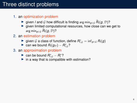
1. an optimization problemI given l and G how difficult is finding argming∈G R̂l(g,D)?I given limited computational resources, how close can we get to
argming∈G R̂l(g,D)?2. an estimation problem
I given G a class of function, define R∗l,G = infg∈G Rl(g)I can we bound Rl(gD)− R∗l,G?
3. an approximation problemI can be bound R∗l,G − R∗l ?I in a way that is compatible with estimation?
Focus of this courseI the estimation problemI and then the approximation problemI with a few words about the optimization problem
6

Three distinct problems
1. an optimization problemI given l and G how difficult is finding argming∈G R̂l(g,D)?I given limited computational resources, how close can we get to
argming∈G R̂l(g,D)?2. an estimation problem
I given G a class of function, define R∗l,G = infg∈G Rl(g)I can we bound Rl(gD)− R∗l,G?
3. an approximation problemI can be bound R∗l,G − R∗l ?I in a way that is compatible with estimation?
Focus of this courseI the estimation problemI and then the approximation problemI with a few words about the optimization problem
6

Outline
Introduction
PAC learning
ERM in practice
7

A simplified case
Learning conceptsI a concept c is a mapping from X to Y = {0,1}I in concept learning, the loss function lb with lb(p, t) = 1p 6=t
I we consider only a distribution DX over XI risk and empirical risk definitions are adapted to this setting:
I risk: R(g) = EX∼DX (1g(X) 6=c(X))
I empirical risk: R̂(g,D) = 1N
∑Ni=1 1g(Xi ) 6=c(Xi )
I in essence the pair (DX , c) replaces D: this corresponds to anoise free situation
I as a consequence a data set is D = {X1, . . . ,XN} and has tocomplemented by a concept to learn
8

PAC learning
NotationsIf A is a learning algorithm, then A(D) is the model produced byrunning A on the data set D
DefinitionA concept class C (i.e. a set of concepts) is PAC-learnable if there isan algorithm A and a function NC from [0,1]2 to N such that: for any1 > ε > 0 and any 1 > δ > 0, for any distribution DX and any conceptc ∈ C, if N ≥ NC(ε, δ) then
PD∼DNX{R (A(D)) ≤ ε} ≥ 1− δ
I probably ≥ 1− δI approximately correct ≤ ε
9

Concept learning and ERM
RemarkI the concept to learn c is in CI thus R∗G = 0
I in addition, for any D, R̂(gERM,G,D,D) = 0I then ERM provides PAC-learnability if for any g ∈ C such that
R̂(g,D) = 0, PD∼DNX{R (g) ≤ ε} ≥ 1− δ
TheoremLet C be a finite concept class and let A be an algorithm that outputsA(D) such that R̂(A(D),D) = 0. Then when N ≥
⌈1ε log |C|δ
⌉,
PD∼DNX{R (A(D)) ≤ ε} ≥ 1− δ
10

Proof
1. we consider ways to break the AC part, i.e. having bothR̂(g,D) = 0 and R(g) > ε. We have
Q = P(∃g ∈ C, R̂(g,D) = 0 and R(g) > ε) =
P
⋃g∈C
(R̂(g,D) = 0 and R(g) > ε
)2. union bound Q ≤
∑g∈C P(R̂(g,D) = 0 and R(g) > ε)
3. then we have
P(R̂(g,D) = 0 and R(g) > ε) = P(R̂(g,D) = 0|R(g) > ε)P(R(g) > ε)
≤ P(R̂(g,D) = 0|R(g) > ε)
11
Proof cont.
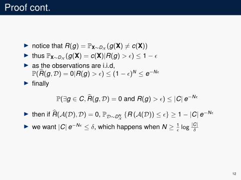
I notice that R(g) = PX∼DX (g(X) 6= c(X))
I thus PX∼DX (g(X) = c(X)|R(g) > ε) ≤ 1− εI as the observations are i.i.d,
P(R̂(g,D) = 0|R(g) > ε) ≤ (1− ε)N ≤ e−Nε
I finally
P(∃g ∈ C, R̂(g,D) = 0 and R(g) > ε) ≤ |C|e−Nε
I then if R̂(A(D),D) = 0, PD∼DNX{R (A(D)) ≤ ε} ≥ 1− |C|e−Nε
I we want |C|e−Nε ≤ δ, which happens when N ≥ 1ε log |C|δ
12

PAC concept learning
ERMI ERM provides PAC-learnability for finite concept classesI optimization computational cost in Θ (N |C|)
Data consumptionI the data needed to reach some PAC level grows with the logarithm
of the concept classI a finite set C can be encoded with log2 |C| bits (by numbering the
elements)I each observation X fixes one bit of the solution
13

Generalization
Concept learning is too limitedI no noiseI fixed loss function
Agnostic PAC learnabilityA class of models G (functions from X to Y) is PAC-learnable withrespect to a loss function l if there is an algorithm A and a function NGfrom [0,1]2 to N such that: for any 1 > ε > 0 and any 1 > δ > 0, forany distribution D on X × Y if N ≥ NG(ε, δ) then
PD∼DN
{Rl (A(D)) ≤ R∗l,G + ε
}≥ 1− δ
Main questionsI does ERM provide agnostic PAC learnability?I does that apply to infinite classes of models?
14
Uniform approximation
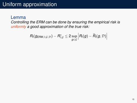
LemmaControlling the ERM can be done by ensuring the empirical risk isuniformly a good approximation of the true risk:
Rl (gERM,l,G,D)− R∗l,G ≤ 2 supg∈G
∣∣∣Rl (g)− R̂l (g,D)∣∣∣
Proof.for any g ∈ G, we have
Rl (gERM,l,G,D)− Rl (g) = Rl (gERM,l,G,D)− R̂l (gERM,l,G,D,D) + R̂l (gERM,l,G,D,D)− Rl (g),
≤ Rl (gERM,l,G,D)− R̂l (gERM,l,G,D,D) + R̂l (g,D)− Rl (g),
≤∣∣∣Rl (gERM,l,G,D)− R̂l (gERM,l,G,D,D)
∣∣∣ + ∣∣∣R̂l (g,D)− Rl (g)∣∣∣ ,
≤ 2 supg∈G
∣∣∣Rl (g)− R̂l (g,D)∣∣∣ ,
which leads to the conclusion.
15

Uniform approximation
LemmaControlling the ERM can be done by ensuring the empirical risk isuniformly a good approximation of the true risk:
Rl (gERM,l,G,D)− R∗l,G ≤ 2 supg∈G
∣∣∣Rl (g)− R̂l (g,D)∣∣∣
Proof.for any g ∈ G, we have
Rl (gERM,l,G,D)− Rl (g) = Rl (gERM,l,G,D)− R̂l (gERM,l,G,D,D) + R̂l (gERM,l,G,D,D)− Rl (g),
≤ Rl (gERM,l,G,D)− R̂l (gERM,l,G,D,D) + R̂l (g,D)− Rl (g),
≤∣∣∣Rl (gERM,l,G,D)− R̂l (gERM,l,G,D,D)
∣∣∣ + ∣∣∣R̂l (g,D)− Rl (g)∣∣∣ ,
≤ 2 supg∈G
∣∣∣Rl (g)− R̂l (g,D)∣∣∣ ,
which leads to the conclusion.
15

Finite classes
TheoremIf |G| <∞ and if l ∈ [a,b] them when N ≥
⌈log( 2|G|
δ )(b−a)2
2ε2
⌉
PD∼DNX
{supg∈G
∣∣∣Rl (g)− R̂l (g,D)∣∣∣ ≥ ε} ≤ 1− δ
Proof.very rough sketch
1. we use the union technique to focus on a single model g
2. then we use the Hoeffding inequality to bound the difference between an empirical averageand an expectation. In our context it says
PD∼DNX
{∣∣∣Rl (g)− R̂l (g,D)∣∣∣ ≥ ε} ≤ 2 exp
(−2N
ε2
(b − a)2
)
3. the conclusion is obtained as in the simple case of concept learning
16

Finite classes
TheoremIf |G| <∞ and if l ∈ [0,1] the ERM provides agnostic PAC-learnability
with NG(ε, δ) =
⌈2 log( 2|G|
δ )(b−a)2
ε2
⌉DiscussionI obvious consequence of the uniform approximation resultI the limitation l ∈ [a,b] can be lifted but only asymptoticallyI the dependency of the data size to the quality (i.e. to ε) is far less
satisfactory than in the simple case: this is a consequence ofallowing noise
17

Infinite classes
RestrictionI we keep the noise but move back to a simple caseI Y = {0,1} and l = lb
Growth functionI if {v1, . . . , vm} is a finite subset of X
G{v1,...,vm} = {(g(v1), . . . ,g(vm)) | g ∈ G} ⊂ {0,1}m
I the growth function of G is
SG(m) = sup{v1,...,vm}⊂X
∣∣G{v1,...,vm}∣∣
18

Interpretation
Going back to finite thingsI∣∣G{v1,...,vm}
∣∣ gives the number of models as seen by the inputs{v1, . . . , vm}
I it corresponds to the number of possible classification decisions(a.k.a. binary labelling) of those inputs
I the growth function corresponds to the worst case analysis: theset of inputs that can be labelled in the largest number of differentways
VocabularyI if
∣∣G{v1,...,vm}∣∣ = 2m then {v1, . . . , vm} is said to be shattered by G
I SG(m) is the m-th shatter coefficient of G
19

Uniform approximation
TheoremFor any 1 > ε > 0 and any 1 > δ > 0 and for any distribution D
PD∼DNX
{supg∈G
∣∣∣Rlb (g)− R̂lb (g,D)∣∣∣ ≥ 4 +
√log(SG(2N))
δ√
2N
}≤ 1− δ
ConsequencesI strong link between the growth function and uniform approximationI useful only if log(SG(2m))
m goes to zero when m→∞I if G shatters sets of arbitrary sizes log(SG(2m)) = 2m log 2
20

Vapnik Chervonenkis dimension
VC-dimension
VCdim(G) = sup {m ∈ N | SG(m) = 2m}
CharacterizationVCdim(G) = m if and only if
1. there is a set of m points {v1, . . . , vm} that is shattered by G2. no set of m + 1 points {v1, . . . , vm+1} is shattered by G
Lemma (Sauer)If VCdim(G) <∞, for all m SG(m) ≤
∑VCdim(G)k=0
(mk
). In particular when
m ≥ VCdim(G)
SG(m) ≤(
emVCdim(G)
)VCdim(G)
21

Finite VC-dimension
ConsequencesIf VCdim(G) = d <∞, for any 1 > ε > 0 and any 1 > δ > 0 and forany distribution D, if N ≥ d then
PD∼DNX
supg∈G
∣∣∣Rlb (g)− R̂lb (g,D)∣∣∣ ≥ 4 +
√log( 2eN
d )
δ√
2N
≤ 1− δ
LearnabilityI a finite VC-dimension ensures agnostic PAC-learnability of the
ERMI it can be shown that NG(ε, δ) = Θ
(VCdim(G)+log 1
δ
ε2
)
22

VC-dimension
VC-dimension calculation is very difficult! A useful result:
TheoremLet F be a vector space of functions from X to R of dimension p. Let Gbe the class of models given by
G ={
g : X → {0,1} | ∃f ∈ F ,∀X ∈ X g(X) = 1f (X)≥0}.
Then VCdim(G) ≤ p.
23

Is a finite VC-dimension needed?
TheoremLet G be a class of models from X to Y = {0,1}. Then the followingproperties are equivalent:
1. G is agnostic PAC-learnable with the binary loss lb2. ERM provides agnostic PAC-learnable with the binary loss lb for G3. VCdim(G) <∞
InterpretationI learnability in the PAC sense is therefore uniquely characterized
by the VC-dimension of the class of modelsI no algorithmic tricks can be used to circumvent this fact!I but this applies only to a fix class!
24

Beyond binary classification
I numerous extensions are availableI to the regression setting (with quadratic or absolute loss)I to classification with more than two classes
I refined complexity measures are availableI Rademacher complexityI Covering numbers
I better bounds are also availableI in generalI in the noise free situation
But the overall message remains the same: learnability is only possiblein classes of bounded complexity.
25

Outline
Introduction
PAC learning
ERM in practice
26
ERM in practice
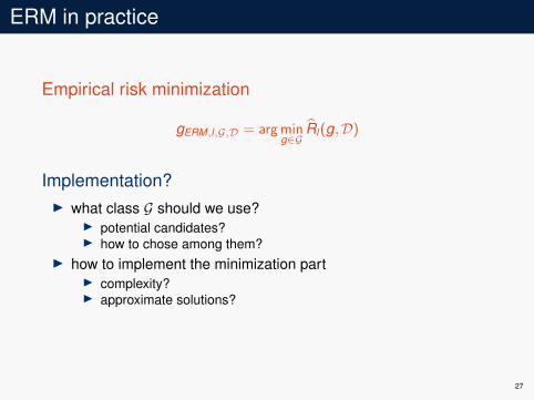
Empirical risk minimization
gERM,l,G,D = arg ming∈G
R̂l (g,D)
Implementation?I what class G should we use?
I potential candidates?I how to chose among them?
I how to implement the minimization partI complexity?I approximate solutions?
27

Model classes
Some examplesI fixed “basis” models, e.g. for Y = {−1,1}
G =
{X 7→ sign
(K∑
k=1
αk fk (X)
)},
where the fk are fixed functions from X to RI parametric “basis” models
G =
{X 7→ sign
(K∑
k=1
αk fk (wk ,X)
)},
where the fk (wk , .) are fixed functions from X to R and the wk areparameters that enable tuning the fk
I useful also for Y = R (remove the indicator function)
28

Examples
Linear modelsI X = RP
I the linearity is with respect to α
I basic modelI fk (X) = XkI∑P
k=1 αk fk (X) = αT XI general models
I fk (X) can be any polynomial function on RP or more generally afunction from RP to R
I e.g. fk (X) = X1X 22 , fk (X) = logX3, etc.
29
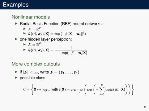
Examples
Nonlinear modelsI Radial Basis Function (RBF) neural networks:
I X = RP
I fk ((β,wk ),X) = exp(−β‖X−wk‖2)
I one hidden layer perceptron:I X = RP
I fk ((β,wk ),X) =1
1 + exp(−β −wTk X)
More complex outputsI if |Y| <∞, write Y = {y1, . . . , yL}I possible class
G =
{X 7→ yt(X), with t(X) = argmax
l
(exp
(−
K∑k=1
αkl fkl(wkl ,X)
))}
30

(Meta)Parameters
Parametric viewI previous classes are described by parametersI ERM is defined at the model level but can equivalently be
considered at the parameter level
I if e.g. G ={
X 7→ sign(∑K
k=1 αk fk (X))}
solving ming∈G R̂lb (g,D) is
equivalent to solving minα∈RK R̂lb (gα,D), where gα is the modelassociated to α
Meta-parametersI to avoid confusion, we use the term "meta-parameters" to refer to
parameters of the machine learning algorithmI in ERM, those are class level parameters (G itself):
I KI the fk functionsI the parametric form of fk (wk , .)
31

ERM and optimization
Standard optimization problemI computing arg ming∈G R̂l (g,D) is a classical optimization problemI no closed-form solution in generalI ERM relies on standard algorithms: gradient based algorithms if
possible, combinatorial optimization tools if needed
Very different complexitiesI from easy cases: linear models with quadratic lossI to NP-hard ones: binary loss even with super simple models
32

Linear regression
ERM version of linear regressionI class of models
G ={
g : RP → R | ∃(β0,β),∀X ∈ RP gβ0,β(x) = β0 + βT x}
I loss: l(p, t) = (p − t)2
I empirical risk: R̂l (gβ0,β,D) = 1N
∑Ni=1
(Yi − β0 − βT Xi
)2
I standard solution(β∗0 ,β
∗)T=(XTX
)−1 XTY with
X =
1 XT1
· · · · · ·1 XT
N
Y =
Y T1· · ·Y T
N
I computational cost in Θ
(NP2
)33

Linear classification
Linear model with binary lossI class of models
G ={
g : RP → {0, 1} | ∃(β0,β), ∀X ∈ RP gβ0,β(x) = sign(β0 + βT x)}
I loss: lb(p, t) = 1p 6=t
I empirical risk: misclassification rateI in this context ERM is NP-hard and tight approximations are also
NP-hardI notice that the input dimension is the source of complexity
NoiseI if the optimal model makes zero error, then ERM is polynomial!I complexity comes from both noise and the binary loss
34

Gradient descent
Smooth functionsI Y = RI parametric case G = {X 7→ F (w,X)}I assume the loss function l and the models in the class G are
differentiable (can be extended to subgradients)I gradient of the empirical loss
∇wR̂l (w,D) =1N
N∑i=1
∂l∂p
(F (w,Xi ),Yi )∇wF (w,Xi )
I ERM through standard gradient based algorithms, such asgradient descent
wt = wt−1 − γt∇wR̂l (wt−1,D)
35

Stochastic gradient descent
Finite sumI leverage the structure of R̂l (w,D) = 1
N
∑Ni=1 l(F (w,Xi ),Yi )
I what about updating according to only one example?I stochastic gradient descent
1. start with a random w0
2. iterate2.1 select i t randomly uniformly in {1, . . . ,N}2.2 wt = wt−1 − γt ∂l
∂p (F (wt−1,Xi t ),Yi t )∇wF (wt−1,Xi t )
I practical tips:I use the Polyak-Ruppert averaging: wm = 1
m
∑m−1t=0 wt
I γ t = (γ0 + t)−κ, κ ∈]0.5, 1], γ0 ≥ 0I numerous acceleration techniques such as momentum (“averaged"
gradients)
36

Ad hoc methods
HeuristicsI numerous heuristics have been proposed for ERM and related
problemsI one of the main tools is alternate/separate optimization: optimize
with respect to some parameters while holding the other constants
Radial basis functionI G =
{X 7→
∑Kk=1 αk exp
(−β‖X−wk‖2
)}I set β heuristically, e.g. to the inverse of the smallest squared
distance between two X in the data setI set the wk via a unsupervised method applied to the (Xi )1≤i≤N
only (for instance the K-means algorithm)I consider β and the wk fixed and apply standard ERM to the αk ,
e.g. linear regression if the loss function is quadratic and Y = R
37
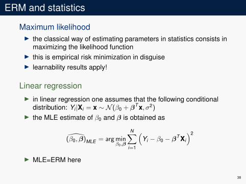
ERM and statistics
Maximum likelihoodI the classical way of estimating parameters in statistics consists in
maximizing the likelihood functionI this is empirical risk minimization in disguiseI learnability results apply!
Linear regressionI in linear regression one assumes that the following conditional
distribution: Yi |Xi = x ∼ N (β0 + βT x, σ2)
I the MLE estimate of β0 and β is obtained as
(̂β0,β)MLE = arg minβ0,β
N∑i=1
(Yi − β0 − βT Xi
)2
I MLE=ERM here
38

Logistic Regression
MLEI in logistic regression one assumes that (with Y = {0,1})
P(Yi = 1|Xi = x) =1
1 + exp(−β0 − βT x)= hβ0,β(x)
I the MLE estimate is obtained by maximizing over (β0,β) thefollowing function
N∑i=1
(Yi log hβ0,β(Xi ) + (1− Yi ) log(1− hβ0,β(Xi )))
39
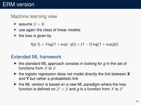
ERM version
Machine learning viewI assume Y = RI use again the class of linear modelsI the loss is given by
l(p, t) = t log(1 + exp(−p)) + (1− t) log(1 + exp(p))
Extended ML frameworkI the standard ML approach consists in looking for g in the set of
functions from X to YI the logistic regression does not model directly the link between X
and Y but rather a probabilistic linkI the ML version is based on a new ML paradigm where the loss
function is defined on Y ′ × Y and g is a function from X to Y ′
40

Relaxation
Simplifying the ERMI ERM with binary loss is complex: non convex loss with no
meaningful gradientI goal: keep the binary decision but remove the binary lossI solution:
I ask to the model a score rather than a binary decisionI build a loss function that compares a score to the binary decisionI use a decision technique consistent with the scoreI generally simpler to formulate with Y = {−1, 1} and the sign function
I this a relaxation as we do not look anymore for a crisp 0/1 solutionbut for a continuous one
41
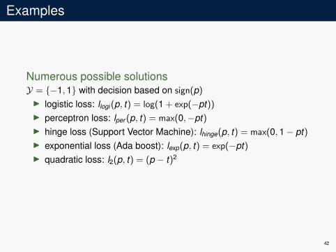
Examples
Numerous possible solutionsY = {−1,1} with decision based on sign(p)
I logistic loss: llogi (p, t) = log(1 + exp(−pt))
I perceptron loss: lper (p, t) = max(0,−pt)I hinge loss (Support Vector Machine): lhinge(p, t) = max(0,1− pt)I exponential loss (Ada boost): lexp(p, t) = exp(−pt)I quadratic loss: l2(p, t) = (p − t)2
42

Beyond ERM
This is not ERM anymore!I sign ◦g is a model in the original sense (a function from X to Y)I but lrelax (g(X),Y ) 6= lb(sign(g(X)),Y)
I surrogate loss minimizationI some theoretical results are availableI but in general no guarantee to find the best model with a surrogate
loss
Are there other reasons to avoid ERM?
43
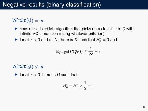
Negative results (binary classification)
VCdim(G) =∞I consider a fixed ML algorithm that picks up a classifier in G with
infinite VC dimension (using whatever criterion)I for all ε > 0 and all N, there is D such that R∗G = 0 and
ED∼DN (R(gD)) ≥ 12e− ε
VCdim(G) <∞I for all ε > 0, there is D such that
R∗G − R∗ >12− ε
44

Conclusion
SummaryThe empirical risk minimization framework seems appealing at first butit has several limitationsI the binary loss is associated to practical difficulties:
I implementation is difficult (because of the lack of smoothness)I complexity can be high in the case of noisy data
I learnability is guaranteed butI only for model classes with finite VC dimensionI which are strictly limited!
Beyond ERMI surrogate loss functionI data adaptive model class
45

Licence
This work is licensed under a Creative CommonsAttribution-ShareAlike 4.0 International License.
http://creativecommons.org/licenses/by-sa/4.0/
46

Version
Last git commit: 2021-01-19By: Fabrice Rossi ([email protected])Git hash: 97cfd0a9975cf193f5790845c00e476c1572a327
47

Changelog
I January 2018: initial version
48