NBER WORKING PAPER SERIES

EMPIRICAL TOOLS AND COMPETITION ANALYSIS:PAST PROGRESS AND CURRENT PROBLEMS

Ariel Pakes

Working Paper 22086http://www.nber.org/papers/w22086

NATIONAL BUREAU OF ECONOMIC RESEARCH1050 Massachusetts Avenue

Cambridge, MA 02138March 2016

This is a revised version of my Laffont lecture, given at the 2015 CRESSE conference, Crete. I thank the editor and a referee for extensive helpful comments. The views expressed herein are those of the author and do not necessarily reflect the views of the National Bureau of Economic Research.

NBER working papers are circulated for discussion and comment purposes. They have not been peer-reviewed or been subject to the review by the NBER Board of Directors that accompanies official NBER publications.

© 2016 by Ariel Pakes. All rights reserved. Short sections of text, not to exceed two paragraphs, may be quoted without explicit permission provided that full credit, including © notice, is given to the source.

Empirical Tools and Competition Analysis: Past Progress and Current ProblemsAriel PakesNBER Working Paper No. 22086March 2016JEL No. L1,L4

ABSTRACT

I review a subset of the empirical tools available for competition analysis. The tools discussed are those needed for the empirical analysis of; demand, production efficiency, product repositioning, and the evolution of market structure. Where relevant I start with a brief review of tools developed in the 1990’s that have recently been incorporated into the analysis of actual policy. The focus is on providing an overview of new developments; both those that are easy to implement, and those that are not quite at that stage yet show promise.

Ariel PakesDepartment of EconomicsHarvard UniversityLittauer Room 117Cambridge, MA 02138and NBERapakes@fas.harvard.edu

1 Introduction.

This paper reviews a set of tools that have been developed to enable us to empir-ically analyze market outcomes, focusing on their possible use in formulatingand executing competition policy. I will be more detailed on developmentsthat seem to be less broadly known by the antitrust community (often becausethey have only been recently introduced), and will emphasize problems that arecurrent roadblocks to expanding the purview of empirical analysis of marketoutcomes further.

The common thread in the recent developments has been a focus on incorpo-rating the institutional background into our empirical models that is needed tomake sense of the data used in analyzing the issues of interest. In large part thiswas a response to prior developments in Industrial Organization theory whichused simplified structures to illustrate how different phenomena could occur.The empirical literature tries to use data and institutional knowledge to narrowthe set of possible responses to environmental or policy changes (or the inter-pretations of past responses to such changes). The field was moving from adescription of responses that could occur, to those that were “likely” to occurgiven what the data could tell us about appropriate functional forms, behavioralassumptions, and environmental conditions.

In pretty much every setting this required incorporating

• heterogeneity of various forms into our empirical models,

and, when analyzing market responses it required

• use of equilibrium conditions to solve for variables that firms could changein response to the environmental change of being analyzed.

The difficulties encountered in incorporating sufficient heterogeneity and/orusing equilibrium conditions differed between what was traditionally viewed as“static” and “dynamic” models. The textbook distinction between these two wasthat: (i) static models analyze price (or quantity) setting equilibria and solve forthe resultant profits conditional on state variables, and (ii) dynamics analyzesthe evolution of those state variables (and through that the evolution of marketstructure). The phrase ”state variables” typically referred to properties of themarket that could only be changed in the medium to long run: the characteristicsof the products marketed, the determinants of costs, the distribution of consumer

3

characteristics, any regulatory or other rules the agents must abide by, and soon.

This distinction has been blurred recently by several authors who note thatthere are a number of industries in which products of firms already in the marketcan be ”repositioned” (can change one or more characteristic) as easily (or al-most as easily) as they can change prices, and then shown that in these industriesstatic analysis of an environmental change that does not take into account thisrepositioning is likely to be misleading, even in the very short run. The prod-uct repositioning literature also employs different empirical tools than had beenused to date, and the tools are relatively easy for competition analysis to accessand use. So between the static and dynamic sections I will include a sectionon ”product repositioning” in which; (iii) incumbents are allowed to repositioncharacteristics of the products they market.

2 Static Models.

The empirical methodology for the static analysis typically relied on earlierwork by our game theory colleagues for the analytic frameworks we used. Theassumptions we took from our theory colleagues included the following:

• Each agent’s actions affect all agents’ payoffs, and

• At the “equilibrium” or “rest point”(i) agents have “consistent” perceptions1, and(ii) each agent does the best they can conditional on their perceptions ofcompetitors’ and nature’s behavior.

Our contribution was the development of an ability to incorporate heterogeneityinto the analysis and then adapt the framework to the richness of different realworld institutions.

The heterogeneity appeared in different forms depending on the issue beinganalyzed. When analyzing production efficiency the heterogeneity was neededto rationalize the persistent differences in plant (or firm) level productivity thatemerged from the growing number of data sets with plant (or firm) level dataon production inputs and outputs. The productivity differences generate both

1Though the form in which the consistency condition was required to hold differed across applications.

4

a simultaneity problem resulting from input choices being related to the (un-observed) productivity term and a selection problem as firms who exit are dis-proportionately those with lower productivity. However once these problemsare accounted for, the new data sets enable an analysis of changes in the envi-ronment (e.g; a merger) on: (i) changes in the efficiency of the output alloca-tion among firms, and (ii) the changes in productivities of individual producingunits (Olley and Pakes, 1996). In demand analysis, allowing for observed andunobserved heterogeneity in both product characteristics and in consumer pref-erences enabled us to adapt McFadden’s (1974) seminal random utility model toproblems that arise in the analysis of market demand. In particular allowing forunobserved product characteristics enabled us to account for price endogene-ity in a model with rich distributions of unobserved consumer characteristics.These rich distributions enabled us to both mimic actual choice patterns in theemerging data sets on individual (or household) choices and to seamlessly com-bine that data with aggregate data on market shares prices and distributionalinformation on household attributes (Berry, Levinsohn and Pakes; 1995, 2004).

A major role of equilibrium conditions was to enable an analysis of counter-factuals (e.g.; proposed mergers, regulatory or tax changes, ....). Few believedthat a market’s response to a change in environmental conditions was to imme-diately “jump” to a new equilibrium. On the other hand most also believed thatthe agents would keep on changing their choice variables until an equilibriumcondition of some form was reached; i.e. until each agent was doing the bestthey could given the actions of the other agents. So the Nash condition wasviewed as a “rest point” to a model of interacting agents. Moreover at leastwithout a generally accepted model of how firms learn and adapt to changes inthe environment, it was natural to analyze the counterfactual in terms of such arest point2.

2.1 Demand Models and Nash Pricing Behavior.

This material is reasonably well known so I will be brief. The advances madein demand analysis were focused on models where products were described bytheir characteristics. I start with Berry Levinsohn and Pakes (1995; henceforth

2The equilibrium conditions were also used to: (i) compare the fit of various behavioral models for settingprices of quantities (e.g.; Nevo 2001), and to (ii) generate additional constraints on the relationship between theprimitives and control variables that were often a great help in estimation (e.g. Berry Levinsohn and Pakes, 1995).

5

BLP) model for the utility of agent i would obtain from product j or

Ui,j =∑k

βi,kxj,k + αipj + ξj + εi,j.

Here the xj,k and the ξj are product characteristics. The difference betweenthem is that the xj,k are observed by the analyst and the ξj are not. The βi,k andαi are household characteristics and the fact that they are indexed by i allowsdifferent households to value the same characteristic differently.

Each individual (or household) is assumed to chose the product (the j) thatmaximized its utility (its Ui,j(·)), and aggregate demand was obtained by sim-ply summing over the choices of the individuals in the market (a tactic madepossible by the speed of computers and the advent of simulation estimators; seeMcFadden, 1989, and Pakes and Pollard, 1989). The main advantages of thisframework are that

• Characteristic space enables us to overcome the ”too-many parameters”problem in models where the demand for a given product depended onthe prices of all products marketed (their if J is the number of products,the number of price coefficients needed grows like J2). In characteristicbased models the number of parameters estimated grows with the numberof characteristics.

• The {ξj} account for unobserved product characteristics and enable ananalysis which does not need to condition on all characteristics that matterto the consumer.

• The {βi,k} and {αi} enable us to generate own and cross price elasticitiesthat depend on the similarity of the characteristics and prices of differentproducts. They can be made a function of income and other observedcharacteristics of the consuming unit as well as an unobserved determinantof tastes.

Assume we are studying consumer demand and pricing behavior in a retailmarket, and for simplicity consider a constant marginal cost firm which hasonly one product to sell in this market. It sets its prices to maximize its profitsfrom the sale of this product. Profits are given by p1q1(·)(p1, . . . , pJ)−mc1q1(·)where q1(·) is the quantity demanded (which depends on the prices and char-acteristics of all the competing firms) and mc1 is its marginal cost. As is well

6

known this implies the price setting equation

p1 = mc1 +1

[∂q1/∂p1]/q1= x1β + w1γ + ω1 +

1

[∂q1/∂p1]/q1, (1)

where mc1 = x1β + w1γ + ω1, x1 is the characteristics of the product, w1

observed market wage rates, and ω1 is unobserved ”productivity”3.There are a couple of implications of equation (4) that should be kept in

mind. The implication of this equation that has been used extensively in therelevant literature is that if one believes the pricing model the pricing equationcan be used to back out an estimate of marginal cost4. The second implication,and the one I want to focus on here, stems from the fact that the markup abovecosts in equation (4), that is 1

[∂q1/∂p1]/q1, can be calculated directly from the de-

mand estimates (we do not need to estimate a pricing equation to get it). Thetwin facts that we can get an independent estimate of the markup and that thepricing theory implies that this markup has a coefficient of one in the pricingequation enables a test of the pricing model. In studies where reasonably pre-cise estimates of the demand system are available without invoking the pricingequation, this test should give the researcher an idea of whether it is appropriateto use the Nash pricing equation as a model of behavior.

To illustrate I asked Tom Wollman to use the data underlying his thesis on thecommercial truck market to do the following: (i) use his demand estimates toconstruct the markup term above, (ii) regress the estimated markup on ”instru-ments” to obtain a predicted markup which is not correlated with the productand cost specific unobservables (ξ and ω)5, and (iii) regress the observed priceon the observed cost determinants and this predicted markup.

A summary of his results is reported in table one. There are two majorpoints to note. First, the fit of the equation is extraordinary for a behavioralmodel in economics (that is we are fitting a variable which is chosen by thefirm). Second the coefficient of the markup is very close to one (it is withinone standard deviation of one), indicating that the Nash in prices assumption

3The equilibrium pricing equation has an extra term in models with adverse selection, as is frequently the casein financial and insurance markets. Adverse (or beneficial) selection causes costs to be a function of price andso will cause a derivative of costs with respect to price to enter the price setting equation; see Einav, Jenkins andLevin, 2012.

4Of course, if other sources of cost data are available, and the competition authorities can sometimes requisitioninternal firm reports on costs, they should be incorporated into the analysis.

5The instruments we used were those used by BLP (1995). For a discussion of the performance of alternativeinstruments see Reynaert and Verboven, 2014

7

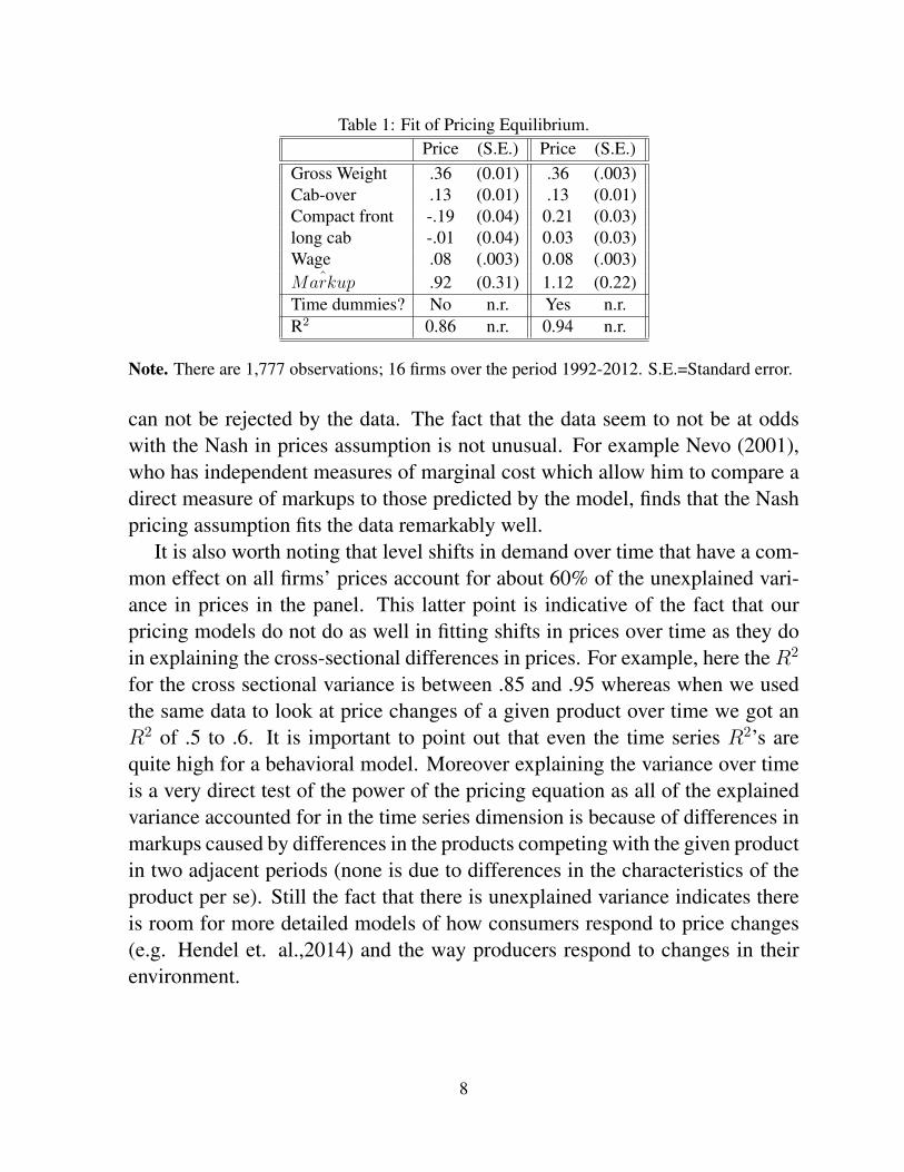
Table 1: Fit of Pricing Equilibrium.Price (S.E.) Price (S.E.)

Gross Weight .36 (0.01) .36 (.003)Cab-over .13 (0.01) .13 (0.01)Compact front -.19 (0.04) 0.21 (0.03)long cab -.01 (0.04) 0.03 (0.03)Wage .08 (.003) 0.08 (.003)

ˆMarkup .92 (0.31) 1.12 (0.22)Time dummies? No n.r. Yes n.r.R2 0.86 n.r. 0.94 n.r.

Note. There are 1,777 observations; 16 firms over the period 1992-2012. S.E.=Standard error.

can not be rejected by the data. The fact that the data seem to not be at oddswith the Nash in prices assumption is not unusual. For example Nevo (2001),who has independent measures of marginal cost which allow him to compare adirect measure of markups to those predicted by the model, finds that the Nashpricing assumption fits the data remarkably well.

It is also worth noting that level shifts in demand over time that have a com-mon effect on all firms’ prices account for about 60% of the unexplained vari-ance in prices in the panel. This latter point is indicative of the fact that ourpricing models do not do as well in fitting shifts in prices over time as they doin explaining the cross-sectional differences in prices. For example, here the R2

for the cross sectional variance is between .85 and .95 whereas when we usedthe same data to look at price changes of a given product over time we got anR2 of .5 to .6. It is important to point out that even the time series R2’s arequite high for a behavioral model. Moreover explaining the variance over timeis a very direct test of the power of the pricing equation as all of the explainedvariance accounted for in the time series dimension is because of differences inmarkups caused by differences in the products competing with the given productin two adjacent periods (none is due to differences in the characteristics of theproduct per se). Still the fact that there is unexplained variance indicates thereis room for more detailed models of how consumers respond to price changes(e.g. Hendel et. al.,2014) and the way producers respond to changes in theirenvironment.

8

Horizontal Mergers and the Unilateral Effects Model. The unilateral effects pricefor a single product firm with constant marginal cost is given by the Nash pricingequilibrium formalized in equation (4) above. The intuition behind that equationis the following: if the firm increases its price by a dollar it gets an extra dollarfrom the consumers who keep purchasing the firm’s product, but it loses themarkup from the consumers who switch out of purchasing the good becauseof the price increase. The firm keeps increasing its price until the two forces’contribution to profits negate each other.

When firm 1 merges with another single product firm, our firm 2, this logicneeds to be modified. Now if the firm increases its price it still gets the extradollar from those who stay, but it no longer loses the markup from every con-sumer who switches out. This because some of the consumers who leave goto what used to be firm 2’s product, and the merged firm captures the markupfrom those who switch to that product. This causes price to increase beyondthe price charged by firm 1 when it only marketed one product. The extent ofincrease depends on the fraction of the customer’s who switch out of firm 1’sproduct that switch to what was firm 2’s product, and the markup on the secondproduct. Formally the post merger price (pm) for firm 2 is written as

pm1 = mc1 +1

[∂q1/∂p1]/q1+ (pm2 −mc2)

∂q2∂p1

/∂q1∂p1

. (2)

The difference between the post merger price in equation (5), our pm, and thepre merger price in (4), our p, has been labelled the ”upward pricing pressure”or ”UPP” (see DOJ and FTC, 2010; and Farrell and Shapiro, 1990). If we let themerger create efficiency gains of E1% in marginal costs we have the followingapproximation6

UPP1 ≈ pm1 − p1 = (p2 −mc2)∂q2∂p1

/∂q1∂p1− E1mc1.

Here ∂q2∂p1/∂q1∂p1

is the fraction of consumers who leave the good owned by firm 1that actually switch to firm 2 and is often called the ”diversion ration”.

The concept of ”UPP” and diversion ratios in merger analysis, like manyother ideas taken from Industrial Organization into antitrust analysis, has beenin graduate class notes for many years. Partly as a result we have had time to

6This is an approximation because the merger will cause a change also in the price of the second good whichshould be factored into an equilibrium analysis. This modifies the formulae (see Pakes, 2011), but not the intuition.

9

consider both when it is appropriate, and the data requirements needed to useit. A full discussion of these issues is beyond what I wanted to do here7, butI did want to stress that the UPP analysis is not always appropriate. This israther obvious when co-ordinated (in contrast to unilateral) behavior is a pos-sibility, so I am going to focus on two more subtle features of the environmentwhich, when present, are likely to make UPP analysis inaccurate. I focus onthese two because a more telling analysis of both of them is now possible. Thefirst, horizontal mergers in vertical markets in which there are a small number ofbuyers and sellers, is discussed in this section. The second, mergers when prod-uct repositioning is likely, is discussed in section 3 which is devoted to productrepositioning.

The basic difference between markets with a small number of buyers andsellers (a buyer-seller network) and retail markets is that in a retail market wegenerally assume that buyers only options are to buy or not buy at the currentprice. In a buyer-seller network the buyer can make a counteroffer to any givenprice; i.e. the buyer can decline to buy at price p but offer to buy at a lowerprice. Negotiations ensue and if a contract is formed it determines how theprofits from the relationship are split8. There is no general agreement on theappropriate equilibrium concept for these markets, though there is agreementthat each agents’ ”outside option” (i.e. the profits it would earn were it not toenter into an agreement) will be a determinant of both which relationships areestablished and the split of the profits among those that are. The implicationof this that is not obvious from the UPP formula (and partly as a result is oftenmistakenly ignored) is that any analysis of a change in the upstream marketmust take account of the structure of the downstream market and visa versa.

The empirical literature has found it most convenient to use Horn and Wolin-sky’s (1988) ”Nash in Nash” assumptions as a basis for the analysis of these sit-uations. In that framework negotiations are bilateral; if two agents contract thesplit of the profits between them is determined by Nash bargaining, and a Nashcondition is imposed on who contracts with whom. The Nash condition is that

7My own discussion of these issues can be found at http://scholar.harvard.edu/pakes/presentations/comments-onupward-pricing-pressure-new-merger-guidelines;.

8There has been a good deal of empirical work recently on other markets where a Nash in price (or quantity)assumption that underlies the UPP analysis is inappropriate.Two others, are markets with repeated auctions suchas those often used by procurement agencies (see Porter, 2015, for an extended discussion). and markets wherethere is a centralized matching mechanism, such as the medical match (see Agarwal, 2015, for a start at analyzingmarket structure issues in these markets).

10

if an agent contracts with another it must earn more profits from the situationgenerated by the contract then it would absent the contract, and visa versa for atleast one agent were the agents not to contract. One questionable assumption isthat the deviations are evaluated under the assumption that no other changes inthe contracting situation would occur in response to the deviation.

The paper that laid the groundwork for empirical work in this area is Craw-ford and Yorukuglu (2013), who analyzed the likely impact of forced de-bundlingof the tiers set by Cable TV providers. The estimate of the resulting change inconsumer welfare differed dramatically by whether the upstream market (themarket between the content providers and the cable networks) was allowed toadjust to the new downstream situation (and many content providers would notsurvive if no realignment of upstream contracts was allowed). Interestingly avariant of their model was also used by the FCC to analyze the likely impactsof the Comcast-NBCU merger9. Since that time related frameworks have beenused to analyze the likely impacts of hospital mergers (Gowrisankaran, G., A.Nevo, and R. Town, 2015), whose impacts on insurance premiums would de-pend on the nature of the downstream premium setting game between insurers,and health insurer mergers (Ho, K. and R. Lee, 2015) whose impact on hospitalprices depended on the nature of the upstream market between insurers and hos-pitals10. The current structural changes in the nature of health care provision inthe United States make this sort of analysis both timely, and economically im-portant.

2.2 Firm and Industry Productivity.

Partly due to various public agencies providing access to Census like files,there has been a marked increase in the availability of data on the inputs andoutputs of production units (firms and/or plants). The advantage over industrylevel data on inputs and outputs is that the micro data has opened up the possi-bility of separating the analysis of the; (i) sources of productivity increases (orcost decreases) in individual plants, from (ii) the role of inter-firm output allo-cations, or market structure, in determining industry productivity. So we noware better able to analyze such traditional IO questions as; the efficiency of the

9See https : //apps.fcc.gov/edocspublic/attachmatch/FCC − 11− 4A1.pdf .10Interestingly, at the time I am writing, the framework set out in this paper being used to analyze mergers in the

U.S. health insurance industry.

11

output allocation, the presence of economies of scale and/or scope, the role ofmarket structure in inducing competitive efficiencies11, spillovers from inven-tive activity, and the effect of infrastructure on the productivity of individualfirms.

Productivity is defined as a measure of output divided by an index of inputs.The input index is typically associated with a production function. Among thesimplest such functions used is the Cobb-Douglas, written as

yi,t = β0 + βlli,t + βkki,t + βmmi,t + ωi,t, (3)

where yi,t is the logarithm of the output measure for firm i in period t, andki,t,mi,t and li,t are the logarithms of the labor, capital, and materials inputsrespectively, while ωi,t is the unobserved productivity term. So if we let uppercase letters be antilogs of their lower case counterparts and B = exp[β0], thenproductivity would be measured as

pi,t =Yi,t

BLβli,tKβki,tM

βMi,t

,

or output per unit of the input index.To construct the productivity measures one needs estimates of the β param-

eters. There are two well known problems in obtaining those estimates fromequation (6). First the input measures are at least partially under the control offirms, and if input prices are approximately the same across firms (or at least notnegatively correlated with productivity), it is in the interest of more productivefirms to use larger quantities of those inputs. This generates a positive cor-relation between input quantities and the unobserved productivity term whichgenerates the estimation problem often referred to as ”simultanaeity”.

Second, basic economics tells us that higher productivity firms and firmswith more capital should be more highly valued and, at least absent a perfectmarket for those inputs, be less likely to exit. As a result highly capitalizedfirms who exit tend to have disproportionately low productivity and poorly cap-italized firms who continue tend to have disproportionately high productivity.This ”natural selection” process will; (i) cause a correlation between the pro-ductivities and capital of continuing firms, and (ii) will generate a bias in ourestimates of the productivity effects of any given environmental change. The

11For a review of the empirical findings on this, see Holmes and Schmitz, 2010

12

bias in our measure of productivity changes results from firms whose produc-tivity was negatively impacted by the change exit and, as a result, the impact ofthe environmental change on their productivity is not measured. The selectioneffects are often particularly large when, as is often the case, we are investigat-ing the effects of a major environmental change (e.g., the impacts of a majorregulatory change).

Olley and Pakes (1996) show how use of the implications of equilibriumbehavior, both for the choice of inputs and for the decisions of when to exit, canbe used by the researcher to circumvent the resulting estimation problems12.The implementation is made significantly easier and less subject to particularassumptions through use of advances in semi-parameteric estimation techniques(see Powell, 1994, and the literature cited their). Olley and Pakes (1996) alsopropose an intuitive way of decomposing industry wide productivity, defined asthe share weighted average of firm level productivity. Industry productivity (sayPt) is equal to the sum of (i) a term measuring the efficiency of the allocationof output among firms, and (ii) the average of individual firm productivities.Formally

Pt =∑i

pi,tsi,t = pt +∑i

∆pi,t∆si,t,

where: pt is the (unweighted) average productivity, ∆pi,t = pi,t−pt, and ∆si,t isthe firm’s share minus the average share. So the term measuring the efficiencyof the output allocation is the covariance between share and productivity acrossfirms in the industry (more precisely the numerator of that covariance)13 .

The empirical content of the Olley and Pakes (1996) article is also of someinterest to the study of antitrust. They analyze the evolution of productivityin the telecommunication equipment industry before and after the breakup ofA.T.&T and the divestment of its wholly owned equipment subsidiary, WesternElectric (the consent decree was filed in 1982 and the breakup and divestmentwere complete by 1984). They find industry wide productivity growth between3 to 4% during the period from 1978 to 1987 (this includes a large fall in pro-ductivity during an adjustment period of 1981-83). Perhaps more important toregulatory economics, the industry’s productivity increases, which were accel-

12For a detailed treatment of this estimation procedure, and the improvements that have been made to it, see thesection 2 of Ackerberg, Benkard, Berry, and Pakes (2007).

13For a dynamic version of this decomposition which explicitly considers the contributions of entrants andexitors in change in Pt over time see Melitz and Polanec, 2015.

13

erating at the end of the sample period, were: (i) almost entirely caused by thecovariance term in the above formula and, (ii) could largely be attributed to thereallocation of capital to more productive firms (often as a result of the exit ofunproductive firms). That is the entry and selection effects of the increased com-petition that resulted from deregulation accounted for most of the productivityeffects that occurred just after deregulation.

The production data from most data sets contains information from multi-product producing units, a fact which underlies the widespread use of sales rev-enue as the output measure in the productivity analysis (indeed this led Olleyand Pakes to relabel the ”production function” in equation (6) a ”sales gener-ating function”). Though it is of interest to know how environmental changeseffect sales per unit of inputs, it would be of more interest to understand howthose changes effect price and quantity separately. However to do this we wouldneed to either know or be able to construct separate quantity and price measuresfor the different outputs produced by the firm. Jan De Loecker and his coau-thors have used different methods to separate revenue growth into its quantityand price components, and then separately analyze the; (i) growth in markupsand, (ii) growth in the productivity of inputs in decreasing costs (or an approxi-mations thereof). In particular De Loecker and Warzynski (2012) use the inputequilibrium conditions for a perfectly variable factor of production in a pricetaking input market to add a step to the estimation procedure that allows themto separate changes in revenue into: (i) changes in markups, and (ii) productiv-ity related changes in costs.

A good example of the usefulness of this type of analysis appears in a sub-sequent paper by De Loecker, J., P. Goldberg, A. Khandelwal and N. Pavcnik,(forthcoming). They study the impacts of a trade liberalization in India on pro-ductivity prices and costs (the liberalization began in 1991, and they study datafrom 1989 and 1997). There have been a number of prior analysis of the pro-ductivity impacts of trade liberalization but most used a framework in whichmarkups were not allowed to change. The new analysis allowed firm specificmarkups, and analyzed how the markups varied after the tariff change. Thetariff declines lowered both input and output prices. The input price declinesresulted in disproportionate increases in markups, rather than to reductions inconsumer prices; i.e. there was limited pass through of the fall in producer coststo consumer prices (at least during the time period they analyze). The markup

14

increase did induce entry and an increase in the variety of goods available inthe market. An analysis of why this occurred would undoubtedly require moreinstitutional information on the industries studied and more detailed analysis ofthe equilibrium generating the pass through they find. However their study isclearly an important first step in our understanding of how a major change inthe economic environment impacted a large share of the world’s population.

3 Product Repositioning.

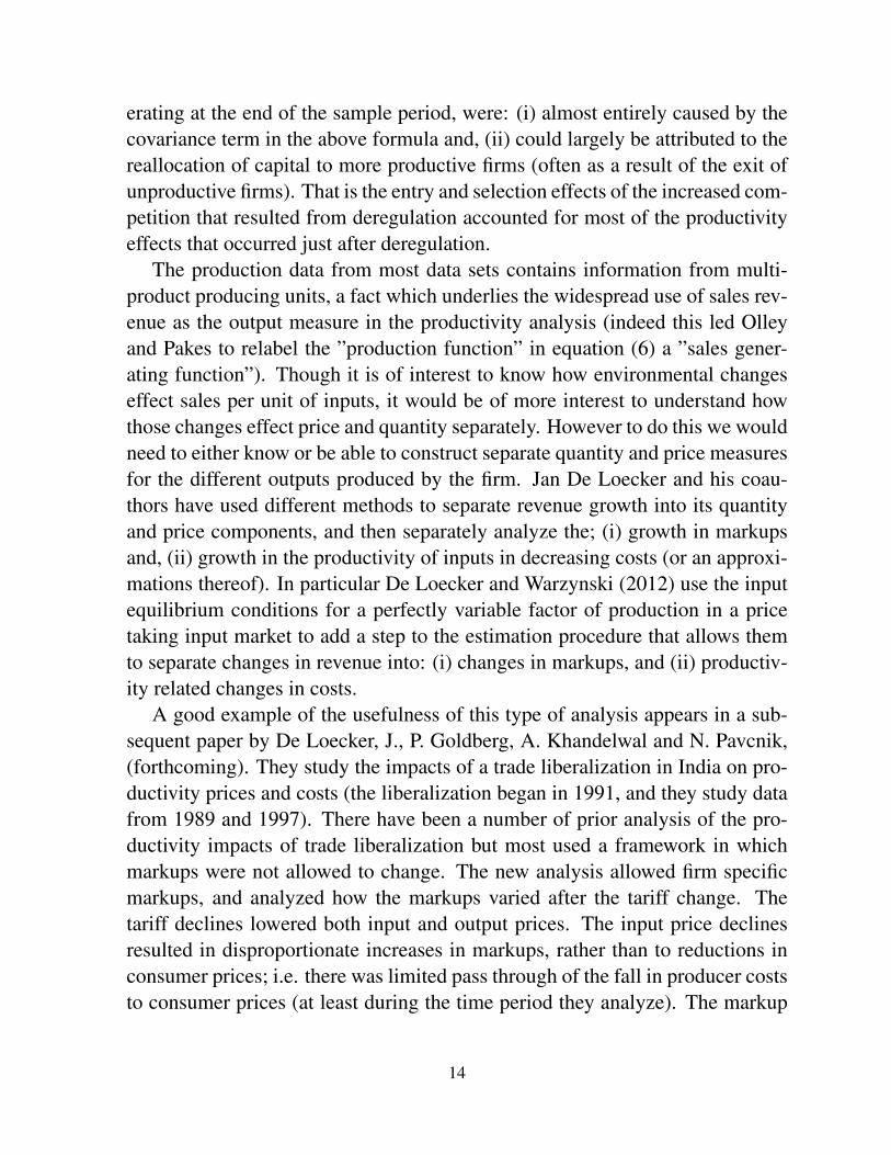
In some industries incumbents can ”reposition” their products as fast, or almostas fast, as prices can be changed. This section considers two period models thatallow us to analyze product repositioning14. The most dramatic illustration ofthe ease of product repositioning that I am aware of is contained in a series offigures in Chris Nosko’s thesis (see Nosko 2014)15.

Nosko analyzes the response of the market for CPU’s in desktop computersto Intel’s introduction of the Core 2 Duo generation of chips. Two firms dom-inate this market: Intel and AMD. Nosko explains that it is relatively easy tochange chip performance provided it is lower than the best performance fromthe current generation of chips. Indeed he shows that chips sold at a given pricetypically change their characteristics about as often as price changes on a givenset of characteristics.

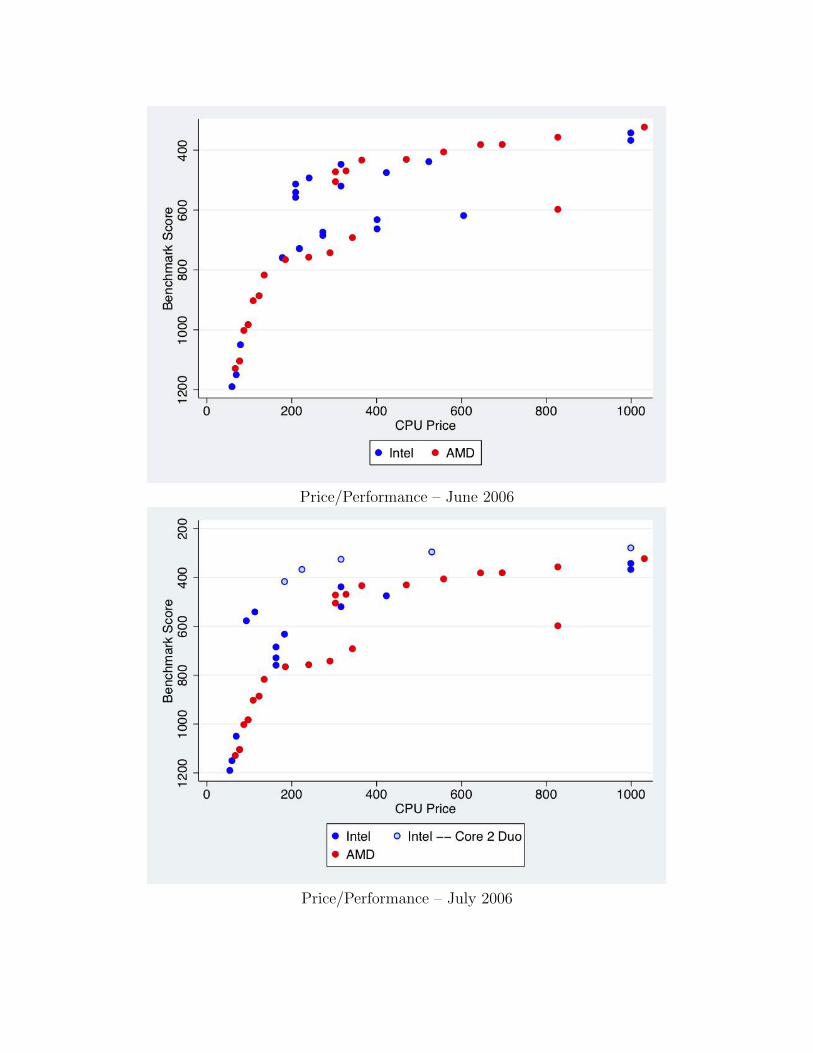
The first figure provides benchmark scores and prices for the products of-fered in June 2006, just prior to the introduction of the Core 2 Duo. The red andblue dots represent AMD’s and Intel’s offerings, respectively. Note that in Junethere was intense competition for high performance chips with AMD selling thehighest priced product at just over $1000. Seven chips sold at prices between$1000 and $600, and another five between $600 and $400. July saw the intro-duction of the Core 2 Duo and figure 2 shows that by October; (i) AMD no

14I want to stress that two period models for the analysis of product repositioning in situations where it isrelatively easy to reposition products is distinct from two period models for the analysis of firm entry. Two periodentry models, as initially set out in Bresnahan and Reiss, 1988, have been incredibly useful as a reduced formway to investigate the determinants of the number of active firms in a market (for more details on the analysis andinterpretation of the results from these models see Pakes, 2014). However, at least in my view, the fact that theiris no history before the first period or future after the second in these models makes its predictions for the impactof an environmental change unreliable for the time horizon relevant for antitrust enforcement. The framework forproduct repositioning presented here conditions on history and is designed specifically to analyze how the industryis likely to respond to such changes.

15I thank him for allowing me to reproduce two of them

15

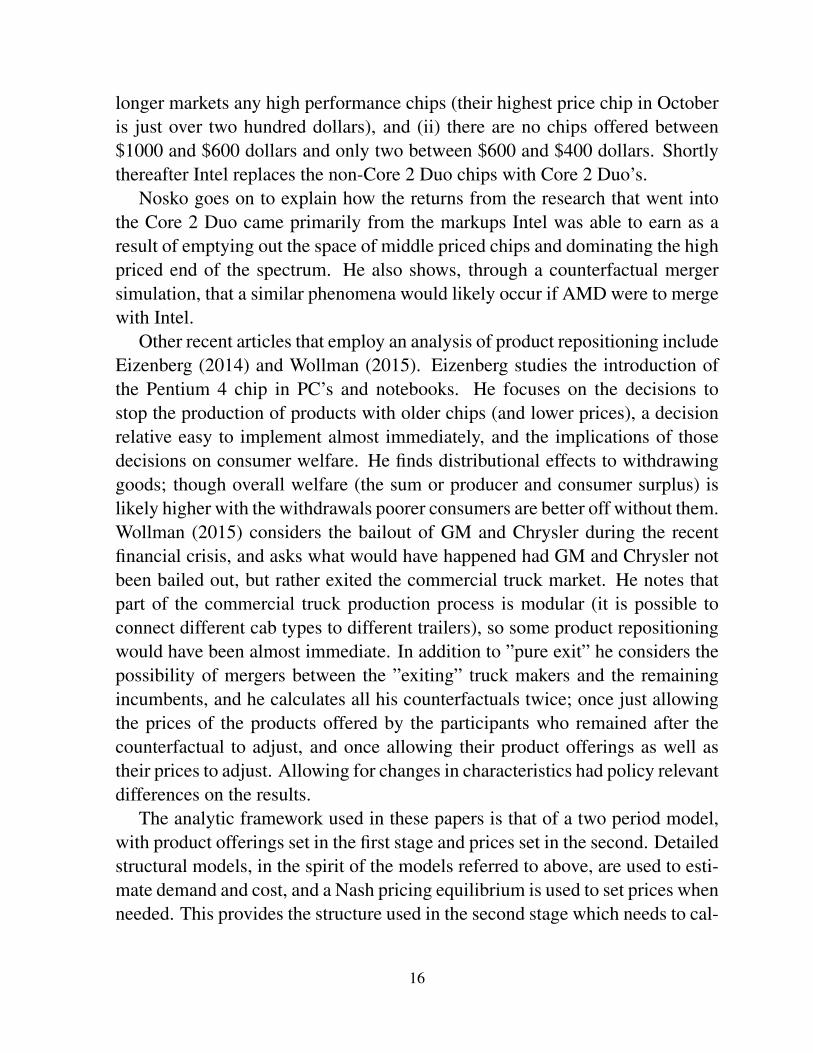
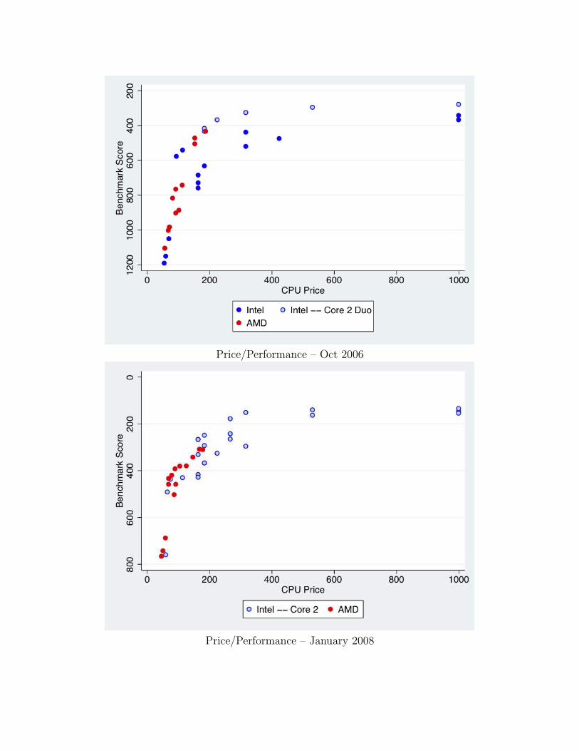
longer markets any high performance chips (their highest price chip in Octoberis just over two hundred dollars), and (ii) there are no chips offered between$1000 and $600 dollars and only two between $600 and $400 dollars. Shortlythereafter Intel replaces the non-Core 2 Duo chips with Core 2 Duo’s.

Nosko goes on to explain how the returns from the research that went intothe Core 2 Duo came primarily from the markups Intel was able to earn as aresult of emptying out the space of middle priced chips and dominating the highpriced end of the spectrum. He also shows, through a counterfactual mergersimulation, that a similar phenomena would likely occur if AMD were to mergewith Intel.

Other recent articles that employ an analysis of product repositioning includeEizenberg (2014) and Wollman (2015). Eizenberg studies the introduction ofthe Pentium 4 chip in PC’s and notebooks. He focuses on the decisions tostop the production of products with older chips (and lower prices), a decisionrelative easy to implement almost immediately, and the implications of thosedecisions on consumer welfare. He finds distributional effects to withdrawinggoods; though overall welfare (the sum or producer and consumer surplus) islikely higher with the withdrawals poorer consumers are better off without them.Wollman (2015) considers the bailout of GM and Chrysler during the recentfinancial crisis, and asks what would have happened had GM and Chrysler notbeen bailed out, but rather exited the commercial truck market. He notes thatpart of the commercial truck production process is modular (it is possible toconnect different cab types to different trailers), so some product repositioningwould have been almost immediate. In addition to ”pure exit” he considers thepossibility of mergers between the ”exiting” truck makers and the remainingincumbents, and he calculates all his counterfactuals twice; once just allowingthe prices of the products offered by the participants who remained after thecounterfactual to adjust, and once allowing their product offerings as well astheir prices to adjust. Allowing for changes in characteristics had policy relevantdifferences on the results.

The analytic framework used in these papers is that of a two period model,with product offerings set in the first stage and prices set in the second. Detailedstructural models, in the spirit of the models referred to above, are used to esti-mate demand and cost, and a Nash pricing equilibrium is used to set prices whenneeded. This provides the structure used in the second stage which needs to cal-

16

Price/Performance – June 2006

Price/Performance – July 2006

Price/Performance – Oct 2006

Price/Performance – January 2008

culate profits for different sets of products. The analysis of the first stage, i.e.the calculation of whether to add (or delete) different products, requires an esti-mate of an additional parameter: the fixed costs of adding or dropping a productfrom the market. It is estimated using the profit inequality approach proposedin Pakes, Porter, Ho and Ishii (2015; henceforth PPHI) and Pakes (2010).

The profit inequality approach is analogous to the revealed preference ap-proach to demand analysis when the choice set is discrerte. To understand howit works assume the fixed costs are the same for adding any product., and letxj = [1, 0]L where L is the number of products that firm j could offer andthe vector xj has a 1 for products offered and a 0 otherwise. Let ez be an L-dimensional vector with one in the ”z” spot and zero elsewhere, and assume thatthe zth product was just added. We use the framework above to compute boththe actual profits and the implied profits had the product not been added16. Let(πj(xj, x−j), πj(xj − ez, x−j)), be the profits with and without marketing thezth product, Ij be the agent’s information set, and E[·|I|] deliver expectationsconditional on Ij. The behavioral assumption is that z was added because

E[πj(xj, x−j)− πj(xj − ez, x−j)|Ij] ≥ F,

where F is the fixed cost of adding a product. If we average over all the productsintroduced and assume expectations are unbiased, we get a consistent lowerbound for F . On the other hand if the zth product is a feasible addition that wasnot offered, and (πj(xj, x−j), πj(xj + ez, x−j) were the profits without and withthat product, then

E[πj(xj + ez, x−j)− πj(xj, x−j), |Ij] ≤ F,

which gives us an upper bound to F .Notice that it is the power of the structural approach to make out of sample

predictions, the same aspect of that approach used in the analysis of mergers,that lets us estimate fixed costs. One feature of this bounds approach to esti-mating fixed costs that makes it attractive in the current context is that it allowsfor measurement error in profits, and this provides partial protection from devi-ations from the assumptions used in constructing the needed counterfactuals17.

16This would have been a unilateral deviation in the first stage simultaneous move game, and hence not changedthe products marketed by other firms.

17This distinguishes the econometric properties of the current mode of analysis from those of the prior literatureon two period entry models; see Pakes, 2014, for more detail.

17

Still there are a number of issues that can arise. First we may want to allow fordifferential fixed costs across products or locations. A straightforward general-ization of what I just described can allow fixed costs to differ as a function ofobservable variables (like product characteristics)18. Things do get more com-plicated when one allows for unobservable factors that generate differences infixed costs and were known to the agents when they made their product choicedecision. This because the products that are provided are likely to have beenpartially selected on the basis of having unobservable fixed costs that were lowerthan average, and those that are not may have been partially selected for havinghigher than average fixed costs. Possible ways for correcting for any bias in thebounds that selection generates are provided in PPHI and in Manski (2003); seeEizenberg (2014) for an application.

One might also worry that the two period model misses the dynamic aspectsof marketing decisions that would arise if F represented sunk, rather than fixed,costs. A more complete analysis of this situation would require the sequentialMarkov equilibrium discussed in the next section. However there is a way topartially circumvent the complexity of Markov equilibria. If it was feasibleto market z but it was not offered and we are willing to assume the firm cancredibly commit to withdrawing it in the next period before competitors nextperiod decisions are taken, then we can still get an upper bound. The upperbound is now to the cost of marketing and then withdrawing the product. I.e.our behavioral assumption now imply that the difference in value between (i)adding a product not added and then withdrawing it in the next period and (ii)marketing the products actually marketed, is less than zero. This implies

E[πj(xj + ez, x−j)− πj(xj, x−j)|Ij] ≤ F + βW.

where W ≥ 0 is the cost of withdrawing and β be the discount rate. Lowerbounds require further assumptions, but the upper bound ought to be enough forexamining extremely profitable repositioning moves following environmentalchanges (like those discussed in Nosko (2011).

Given these bounds we turn to considering likely product repositioning de-cisions that follow an environmental change. Typically if we allow the product

18Though this does require use of estimation procedures from the literature on moment inequality estimators.For an explanation of how these estimators work see Tamer (2010). When there are many parameters that needto be estimated in the fixed cost equation these estimators can become computationally demanding, but their is anactive econometric literature developing techniques which reduce this computational burden, see for e.g. Kaido et.al. 2014.

18

mix of incumbents to adjust as a result of say a merger or an exit there willbe a number of market structures that are Nash equilibria in the counterfactualenvironment (though one should not forget that the number of equilibria will belimited by profitability implications of the investments in place).

There are different ways to analyze counterfactuals when there is the pos-sibility of multiple equilibria. One is to add a model for how firm’s adjust tochanges in their environment and let the adjustment procedure chose the equi-libria (for examples see Lee and Pakes, 2009, and Wollman, 2015). Alterna-tively we could assume that firms’ assume that their competitors do not changethe products they market in the relevant time horizon, and find a best responseto those products given the changed environment19. Another possibility is enu-meration of the possible equilibria (or at least those that seem likely on the basisof some exogenous criteria), and consider properties of all members of that set,as is done in Eizenberg (2014).

4 Dynamics and the Evolution of State Variables.

Empirical work on dynamic models proceeded in a similar way to the way weproceeded in static analysis; we took the analytic framework from our theorycolleagues and tried to incorporate the institutions that seemed necessary toanalyze actual markets. We focused on models where

1. state variables evolve as a Markov process,

2. and the equilibrium was some form of Markov Perfection (no agent has anincentive to deviate at any value of the state variables).

In these models firms chose ”dynamic controls” (investments of different types)and these determine the likely evolution of their state variables. Implicit inthe second condition above is that players’ have perceptions of the controls’likely impact on the evolution of the state variables (their own and those of theircompetitors) and through that on their current and future profits, and that theseperceptions are consistent with actual behavior (by nature, as well as by their

19We could also iterate on this for all competitors to find a rest point to ”iterated” best responses. This is oneway to model the adjustment process. For a theoretical treatment of alternatives see Fudenberg and Levine, 1998,and for an attempt to distinguish between learning algorithms actually used in an industry, see Doraszelski, Lewis,and Pakes, 2015. It is worth mentioning that in a world where there is randomness in the environment, adjustmentprocesses can lead to a probability distribution of possible equilibria.

19

competitors). The standard references here are Maskin and Tirole (1988a andb) for the equilibrium notion and Ericson and Pakes (1995) for the frameworkused in computational theory and empirical work.

The Markov assumption is both convenient and, except in situations involv-ing active experimentation and learning, fits the data well20, so empirical workis likely to stick with it. The type of rationality built into Markov Perfectionis more questionable. It has been useful in correcting for dynamic phenomenain empirical problems which do not require a full specification of the dynamicequilibrium (as in the Olley and Pakes example above),. The Markov Perfectframework also enabled applied theorists to explore possible dynamic outcomesin a structured way. This was part of the goal of the original Maskin and Ti-role articles and computational advances have enabled Marko Perfection to beused in more detailed computational analysis of a number of other issues thatwere both, integral to antitrust analysis, and had not been possible before21.Examples include; the relationship of collusion to consumer welfare when weendogenize investment entry and exit decisions (as well as price, see Fershtmanand Pakes, 2000), understanding the multiplicity of possible equilibria in mod-els with learning by doing (Besanko, Doraszelski, Kryukov and Satterthwaite,2010), and dynamic market responses to merger policy (Mermelstein, Nocke,Satterthwaite, and Whinston 2014).

Perhaps not surprisingly, the applied theory indicated just how many differ-ent outcomes were possible in Markov perfect models, especially if one waswilling to perturb the functional forms or the timing assumptions in those mod-els. This provided additional incentives for empirical work, but though therehas been some compelling dynamic empirical work using the Markov Perfectframework (see for e.g.; Benkard, 2004, Collard-Wexler, 2013, and Kaloupt-sidi, 2014)22, it has not been as forthcoming as one might have hoped. This isbecause the framework becomes unweildly when confronted with the task ofincorporating the institutional background that seemed relevant.

When we try to incorporate the institutional background that seems essential20It also does not impose unrealistic data access and retention conditions for decision making agents.21The computational advances enabled us to compute equilibria quicker and/or with less memory requirements

then in the simple iterative procedure used in the original Pakes and McGuire (1994) article. The advances in-clude; Judd’s (1998) use of deterministic approximation techniques, Pakes and McGuire (2001)’s use of stochasticapproximation, and Doraszelski and Judd (2011)’s use of continuous time to simplify computation of continuationvalues.

22A review by Doraszelski and Pakes, 2000 provides a more complete list of cites to that date.

20

to understanding the dynamics of the market we often find that both the analyst,and the agents we are trying to model, are required to: (i) access a large amountof information (all state variables), and (ii) either compute or learn an unrealisticnumber of strategies. To see just how complicated the dynamics can become,consider a symmetric information Markov Perfect equilibrium where demandhas a forward looking component; as it would if we were studying a durable,storable, experience, or network good.

For specificity consider the market for a durable good. Both consumers andproducers would hold in memory at the very least; (i) the cartesian product ofthe current distribution of holdings of the good across households crossed withhousehold characteristics, and (ii) each firm’s cost functions (one for producingexisting products and one for the development of new products). Consumerswould hold this information in memory, form a perception of the likely prod-uct characteristics and prices of future offerings, and compute a dynamic pro-gramme to determine their choices. Firms would use the same state variables,take consumers decisions as given, and compute their equilibrium pricing andproduct development strategies. Since these strategies would not generally beconsistent with the perceptions that determined the consumers’ decisions, thestrategies would then have to be communicated back to consumers who wouldthen have to recompute their dynamic program using the updated firm strate-gies. This process would need to be repeated until we found strategies whereconsumers do the best they can given correct perceptions of what producerswould do and producers do the best they can given correct perceptions on whateach consumer would do (a doubly nested fixed point calculation). Allowing forasymmetric information could reduce information requirements, but it wouldsubstantially increase the burden of computing optimal strategies. The addi-tional burden results from the need to compute posteriors, as well as optimalpolicies; and the requirement that they be consistent with one another.

There have been a number of attempts to circumvent the computational com-plexity of dynamic problems by choosing judicious functional forms for prim-itives and/or invoking computational approximations. They can be useful butoften have implications which are at odds with issues that we want to study23.

23Examples include Gowrisankaran and Rysman 2012, and Nevo and Rossi, 2008. A different approach istaken in the papers on ”oblivious equilibrium” starting with Benkard et. al. (2012). This was introduced as acomputational approximation which leads to accurate predictions when there were a large number of firms in themarket, but I believe could be reinterpreted in a way that would make it consistent with the framework describedbelow.

21

I want to consider a different approach; an approach based on restricting whatwe believe agents can do. It is true that our static models often endow an agentwith knowledge that they are unlikely to have and then consider the resultantapproximation to behavior to be adequate. However it is hard to believe thatin a dynamic situation like the one considered above, Markov perfection (orBayesian Markov Perfection) is as good an approximation to actual behavioras we can come up with. So I want to consider notions of equilibria whichmight both better approximate agents’ behavior and enable empirical work ona broader set of dynamic issues. This work is just beginning, so I will focus onthe concepts that underlie it and some indication of how far we have gotten.

4.1 Less Demanding Notions of Equilibria.

The framework I will focus on is ”Restricted Experience Based Equilibrium” (orREBE) as described in Fershtman and Pakes (2012). It is similar in spirit to thenotion of ”Self-confirming Equilibrium” introduced in Fudenberg and Levine(1983). The major difference is that REBE uses a different ”state space”, oneappropriate for dynamic games, and as a result has to consider a different set ofissues. There has also been a number of developments of related equilibriumconcepts by economic theorists (see, for example Battigalli, P. et. al, 2015) .

A REBE equilibrium satisfies two conditions which seem natural for a “restpoint” to a dynamical system. They are

1. agents perceive that they are doing the best they can conditional on theinformation that they condition their actions on, and that

2. if the information set that they condition on has been visited repeatedly,these perceptions are consistent with what they have observed in the past.

Notice that this does not assume that agents form their perceptions in any par-ticular way; just that they are consistent with what they have observed in thepast at conditioning sets that are observed repeatedly24.

The state space consists of the information sets the agents playing the gamecondition their actions on. The information set of firm i in period t is denoted

24It might be reasonable to assume more than this, for example that agents know and/or explore properties ofoutcomes of states not visited repeatedly, or to impose restrictions that are consistent with data on the industry ofinterest. We come back to this below where we note that this type of information would help mitigate multiplicityproblems.

22

by Ji,t = {ξt, ωi,t}, where ξt is public information observed by all, and ωi,t isprivate information. The private information is often information on productioncosts or investment activity (and/or its outcomes), and to enhance our ability tomimic data, is allowed to be serially correlated. The public information varieswith the structure of the market. It can contain publicly observed exogenousprocesses (e.g. information on factor price and demand), past publicly observedchoices made by participants (e.g. past prices), and whatever has been revealedover time on past values of ω−i,t.

Firms chose their ”controls” as a function of Ji,t. Since we have allowed forprivate information, these decisions need not be a function of all the variablesthat determine the evolution of the market (it will not depend on the privateinformation of competitors). Relative to a symmetric information Markov equi-librium, this reduces both what the agent needs to keeps track of, and the num-ber of distinct policies the agent needs to form. The model also allows agentsto chose to ignore information that they have access to but think is less relevant(we come back to how the empirical researcher determines Ji,t below).

Typically potential entrants will chose whether to enter, and incumbents willchose whether to remain active and if so their prices and investments (in capital,R&D, advertising, . . .). These choices are made to maximize their perceptionsof the expected discounted value of future net cash flows, but their perceptionsneed not be correct.

The specification for the outcomes of the investment and pricing process,and for the revelation of information, determines the next period’s informationset. For example assume costs are serially correlated and are private informa-tion, and that prices are a function of costs and observed by all participants.Then past price is a signal on current costs, and we would expect all prices inperiod t to be components of ξt+1, the public information in period t + 1. If, inaddition, investment is not observed and it generates a probability distributionfor reductions in cost, then the realization of the cost variable is a component ofωi,t+1, the private information in period t+ 1.

Since agents choices and states are determined by their information sets, the“state” of the industry, which we label as st, is determined by the collection ofinformation sets of the firms within it

st = {J1,t, . . . , Jnt,t} ∈ S.

Assumptions are made which insure that st evolves as a finite state Markov

23

chain. This implies that, no matter the policies, st will wander into a recurrentsubset of the possible states (i.e. of S), and then remain within that subsetforever (Freedman, 1971). Call that subsetR ⊂ S. These states are determinedby the primitives of the market (its size, feasible outcomes from investment,....), and they are visited repeatedly. For example a small market may never seemore than x firms simultaneously active, but in a larger market the maximumfirms ever active may be y > x. Firms in the larger market may flounder andeventually exit, but it is possible that before the number of active firms ever fallsto x there will be entry. Then the recurrent class for the larger market does notinclude Ji,t that are a component of an st that has less than x firms active.

The Ji,t which are the components of the st in R are the information sets atwhich the equilibrium conditions require accurate perceptions of the returns tofeasible actions. So in industries that have been active for some time, neitherthe agent nor the analyst needs to calculate equilibrium values and policies forthe information sets in all of S, we only need them for those in R, and R canbe much smaller than S.

The Fershtman and Pakes (2012) article provide a learning algorithm, in thespirit of reinforcement learning25 that enables the analyst to compute a REBE.Briefly, the algorithm starts at some initial st and has a formulaic method ofgenerating initial perceptions of the expected discounted values of alternativeactions at each possible Ji,t. Each agent choses the action which maximizes itsinitial perceptions of its values. The actions generate a probability distributionover outcomes, and a pseudo random draw from those distributions plus therules on information access determine both the current profit and the new state(our Ji,t+1). Then the current profit and the new state are used to update theperceptions of the values for taking actions in the original state (at Ji,t). Moreprecisely, the profits are taken as a random draw from the possible profits fromthe action taken at the old state, and the new state, or rather the initial percep-tion of the value of the new state, is treated as a random draw from the possiblecontinuation values from the action taken at Ji,t. The random draws on profitsand continuation values are averaged with the old perceptions to form new per-ceptions. This process is then repeated from the new state. So the algorithm isiterative, but each iteration only updates the values and policies at one point (it is”asynchronous”). The policies at that point are used to simulate the next point,

25For an introduction to reinforcement learning see, Sutton, R. and Barto, A. (1998).

24

and the simulated output is used to update perceptions at the old point. Noticethat firms could actually follow these steps to learn their optimal policies, but itis likely to do better as an approximation to how firms react to perturbations intheir environment then to major changes in it26.

This process has two computational advantages. First the simulated processeventually wanders into R and stays their. So the analyst never needs to com-pute values and policies on all possible states, and the states that are in R areupdated repeatedly. Second the updating of perceptions never requires inte-gration over all possible future states, it just requires averaging two numbers.On the negative side there is no guarantee that the algorithm will converge toa REBE. However Fershtman and Pakes program an easy to compute test forconvergence into the algorithm, and if the test output satisfies the convergencecriteria, the algorithm will have found a REBE.

Multiplicity. A Bayesian Perfect equilibrium satisfies the conditions of a REBE,but so do weaker notions of equilibrium. So REBE admits greater multiplicitythan does Bayesian Perfect notions of equilibrium. To explain the major rea-son for the increase in equilibria partition the points in R into “interior” and“boundary” points27. Points in R at which there are feasible (but non-optimal)strategies which can lead outside of R are boundary points. Interior points arepoints that can only transit to other points in R no matter which of the feasiblepolicies are chosen.

The REBE conditions only ensure that perceptions of outcomes are consis-tent with the results from actual play at interior points. Perceptions of outcomesfor feasible (but non-optimal) policies at boundary points need not be tied downby actual outcomes. As a result differing perceptions of discounted values atpoints outside of the recurrent class can support different equilibria. One canmitigate the multiplicity problem by adding either empirical information or by

26This because the current algorithm does not allow for experimentation, and (ii) can require many visits toa given point before reaching an equilibrium (especially when initial and equilibrium perceptions differ greatly).Doraszelski, Lewis and Pakes (2015) study firms learning policies in a new market and find that there is an initialstage where an analogue of this type of learning does not fit, but the learning algorithm does quite well after aninitial period of experimentation.

27This partitioning is introduced in Pakes and McGuire, 2001. There is another type of multiplicity that maybe encountered; there may be multiple recurrent classes for a given equilibrium policy vector. Sufficient conditionfor the policies to generate a process with a unique recurrent class are available (see Freedman, 1971, or Ericsonand Pakes,1995) but there are cases of interest where multiple separate recurrent classes are likely (see Besanko,Doraszeldi and Kryukov, 2014).

25

strengthening the behavioral assumptions.The empirical information should help identify which equilibria has been

played, but may not be of much use when attempting to analyze counterfactu-als. The additional restrictions that may be appropriate include the possibilitythat prior knowledge or past experimentation will endow agents with realisticperceptions of the value of states outside, but close to, the recurrent class. Inthese cases we will want to impose conditions that insure that the equilibria wecompute are consistent with this knowledge. To accommodate this possibility,Asker, Fershtman, Jeon, and Pakes (2015) propose an additional condition onequilibrium play that insures that agents’ perceptions of the outcomes from allfeasible actions from points in the recurrent class are consistent with the out-comes that those actions would generate. They label the new condition ”bound-ary consistency” and provide a computational simple test to determine whetherthe boundary consistency condition is satisfied for a given set of policies.

Empirical Challenges. In addition to the static profit function (discussed in theearlier sections), empirical work on dynamics will require: (i) specifying thevariables in Ji and (ii) estimates of the “dynamic” parameters (these usuallyinclude the costs of entry and exit, and parametric models for both the evolutionof exogenous state variables and the response of endogenous state variables tothe agents’ actions).

There is nothing in our equilibrium conditions that forbids Ji from contain-ing less variables then the decision maker has at its disposal, and a restricted Jimay well provide a better approximation to behavior. The empirical researcher’sspecification of Ji should be designed to approximate how the dynamic controlsare determined (in the simplest model this would include investment, entry andexit policies). This suggests choosing the variables in Ji through an empiri-cal analysis of the determinants of those controls. Information from the actualdecision makers or studies of the industry would help guide this process.

In principle we would like to be able to generate predictions for the dynamiccontrols that replicate the actual decisions up to a disturbance which is a sumof two components; (i) a ”structural” disturbance (a disturbance which is a de-terminant of the agent’s choice, but we do not observe) which is independentlydistributed over time, and (ii) a measurement error component. The measure-ment error component should not be correlated with variables which are thought

26

to be correctly measured, and the structural error should not be correlated withany variable dated prior to the period for which the control is being predicted.So the joint disturbance should be uncorrelated with past values of correctlymeasured variables. This provides one test of whether a particular specificationfor Ji is adequate. If the null is rejected computational and estimation proce-dures which allow for serially correlated errors should be adopted. This neednot pose additional computational problems, but may well complicate the esti-mation issues we turn to now.

Estimates of dynamic parameters will typically be obtained from panel dataon firms, and the increased availability of such data bodes well for this partof the problem. Many of the dynamic parameters can be estimated by carefulanalysis of the relationship between observables; i.e. without using any of theconstructs that are defined by the equilibrium to the dynamic model (such as ex-pected discounted values). For example if investment is observed and directedat improving a given variable, and (a possibly error prone) measure of that vari-able is either observed or can be backed out of the profit function analysis, theparameters governing the impact of the control can be estimated directly.

However there often are some parameters that can only be estimated throughtheir relationship to perceived discounted values (sunk and fixed costs oftenhave this feature). There is a review of the literature on estimating these pa-rameters in the third section of Ackerberg et. al. (2007). It focuses on twostep semi-parameteric estimators which avoid computing the fixed point thatdefines the equilibrium at trial values of the parameter vector28. In additionPakes (2015) describes a “perturbation” estimator, similar to the Euler equationestimator for single agent dynamic problems proposed by Hansen and Singleton(1982). This estimator does not require the first step non-parametric estimator,but is only available for models with asymmetric information. Integrating se-rially correlated unobservables into these procedures can pose additional prob-lems; particularly if the choice set is discrete. There has been recent work ondiscrete choice models that allow for serially correlated unobservables (see Ar-cidiano and Miller, 2011), but it has yet to be used in problems that involveestimating parameters that determine market dynamics.

28The relevant papers here are those of Bajari Benkard and Levin (2007), and Pakes Ostrovsky and Berry,(2007))

27

5 Conclusion.

The advantage of using the tools discussed here to evaluate policies is that theylet the data weigh in on the appropriateness of different functional forms andbehavioral assumptions. Of course any actual empirical analysis will have tomaintain some assumptions and omit some aspects of the institutional environ-ment. The critical issue, however, is not whether the empirical exercise has allaspects of the environment modeled correctly, but rather whether empirics cando better at counterfactual policy analysis than the next best alternative avail-able. Of course in comparing alternatives we must consider only those that;(i) use the information available at the time the decision is made and (ii) abideby the resource constraints of the policy maker. By now I think it is clear thatin some cases empirical exercises can do better than the available alternatives,and that the proportion of such cases is increasing; greatly aided by advances inboth computational power and the resourcefulness of the academic community(particularly young Industrial Organization scholars).

References.• Ackerberg D, L. Benkard, S. Berry, A. Pakes (2007) ”Econometric Tools for Analyzing Market

Outcomes”. In Heckman J, Leamer E, ed., The Handbook of Econometrics Amsterdam: North-Holland, Chapter 63.

• Agarwal, N. (2015) ”An Empirical Model of the Medical Match”, American Economic Review,105(7): 1939-1978.

• Arcidiano, P. and R. Miller (2011) ”Conditional Choice Probability Estimation of Dynamic Dis-crete Choice Models with Unobserved Heterogeneity”, Econometrica, 7(6): 1823-1868.

• Asker, J., C. Fershtman, J. Jeon, and A. Pakes (2014) “The Competitive Effects of InformationSharing”, Harvard University working paper.

• Bajari, P., L. Benkard, and J. Levin (2007) “Estimating Dynamic Models of Imperfect Competi-tion,” Econometrica, 75(5): 13311370 .

• Battigalli, P., S. Cerreia-Vioglio, F. Maccheroni, and M. Marinacci (2015) ”Self-Confirming Equi-librium and Model Uncertainty.” American Economic Review, 105(2): 646-677.

• Benkard, L., (2004) ”A Dynamic Analysis of the Market for Wide-Bodied Commercial Aircraft”Review of Economic Studies, 71(3): 581-611.

• Benkard, L., Van Roy B., and Weintraub G. (2008) ”Markov Perfect Industry Dynamics withMany Firms” Econometrica, 76(6): 1375-1411.

28

• Berry S., J. Levinsohn, and A. Pakes (1995) “Automobile Prices in Market Equilibrium,” Econo-metrica, 63(4): 841-890.

• Berry S., J. Levinsohn, and A. Pakes (2004), “Estimating Differentiated Product Demand Systemsfrom a Combination of Micro and Macro Data: The Market for New Vehicles,” Journal of PoliticalEconomy, 112(1): 68-105.

• Besanko, D., U. Doraszelski, Y. Kryukov, and M. Satterthwaite (2010) ”Learning by Doing, Or-ganizational Forgetting and Industry Dynamics” Econometrica, 78 (2): 453-508.

• Besanko, D., U. Doraszelski, and Y. Kryukov (2014) “The Economics of Predation: What DrivesPricing When There Is Learning-by-Doing?”, American Economic Review, 104(3): 868897.

• Bresnahan, T. and P. Reiss (1988) ”Do Entry Conditions Vary Across Markets”, Brookings Paperson Economic Activity No.3, 833-882.

• Collard-Wexler, A. (2013) ”Demand Fluctuations in the Ready-Mix Concrete Industry”, Econo-metrica, 81(3): 1003-1037.

• Crawford, G. and A. Yurukoglu (2013) “The Welfare Effects of Bundling in Multichannel Televi-sion Markets” American Economic Review, 102(2): 643-85.

• De Loecker J., and Warzynski (2012) ”Markups and Firm-Level Export Status” American Eco-nomic Review, 102(6): 2437-2471.

• De Loecker, J., P. Goldberg, A. Khandelwal and N. Pavcnik, (forthcoming), ”Prices, Markups andTrade Reform” Econometrica.

• Doraszelski, U., and K. Judd (2011) ”Avoiding the Curse of Dimensionality in Dynamic Stochas-tic Games”, Quantitative Economics, 3(1): 53-93.

• Doraszelski U., G. Lewis and A. Pakes (2014) “Just starting out: Learning and price competitionin a new market” mimeo Harvard University.

• Doraszelki, U. and A. Pakes (2008), “A Framework for Applied Dynamic Analysis in I.O.,” in M.Armstrong and R. Porter ed.s. The Handbook of Industrial Organization, Chapter 33, 2183-2262.

• Einav L, M. Jenkins and J. Levin (2012) “Contract Pricing in Consumer Credit Markets” Econo-metrica, 80(4): 1387-1432.

• Eizenberg, A. (2014) ”Upstream Innovation and Product Variety in the United States Home PCMarket,” the Review of Economic Studies, 81(): 1003-1045

• Ericson R. and A. Pakes (1995), “Markov Perfect Industry Dynamics: A Framework for EmpiricalWork,” Review of Economic Studies, 62(1): 53-82.

• Fershtman C. and A Pakes (2000), “A Dynamic Game with Collusion and Price Wars,” RANDJournal of Economics, 31(2): 207-36.

• Fershtman C. and A. Pakes (2012) “Dynamic Games with Asymmetric Information: A Frameworkfor Applied Work” The Quarterly Journal of Economics, 127(4): 1611-1662.

• Fudenberg D. and D. Levine (1983) ”Subgame Perfect Equilibrium of Finite and Infinite HorizonGames” Journal of Economic Theory 31, 227-256.

29

• Fong K. and R. Lee (2013) “Markov Perfect Network Formation: An Appied Framework forBilateral Oligopoly and Bargaining in Buyer-Seller Networks” mimeo Havard University.

• Freedman D. (1971) Markov Chains, Holden Day series in probabilty and statistics.

• Gowrisankaran, G., A. Nevo, and Town, R. (2015) ”Mergers When Prices Are Negotiated: Evi-dence from the Hospital Industry,” American Economic Review, 105(1): 172-203.

• Gowrisankaran, G., and M. Rysman (2012) ”Dynamics of Consumer Demand for New DurableGoods,” Journal of Political Economy, 120(6) 1173-1219.

• Hansen, L. and K. Singleton (1982) ”Generalized Instrumental Variables Estimation of NonlinearRational Expectations Models”, Econometrica, 50(5): 1269-1286.

• Hendel I., S. Lach , and Y. Spiegel (2014) ”Consumers Activism: the Facebook Boycott on Cot-tage Cheese?” CEPR Discussion Paper 10460.

• Hendriks, K, and R. Porter (2015), ”Empirical Analysis and Auction Design” in process North-western University.

• Ho, K, and R. Lee (2015) ”Insurer Competition in Health Care Markets” mimeo Harvard Univer-sity

• Holmes. T. and J. Schmitz (2010) ”Competition and Productivity: A Review of Evidence” AnnualReview of Economics, 619-642.

• Horn H. and A. Wolinsky (1988) ”Bilateral Monopolies and Incentives for Merger” RAND Journalof Economics 19(3): 408-419.

• Judd, K. (1998), Numerical Methods in Economics, MIT Press: Cambridge, MA.

• Kalouptsidi, M. (2014) ”Time to Build and Fluctuations in Bulk Shipping”, American EconomicReview, 104(2): 564-608.

• Kaido, H., Molinari, F. and Stoye, J. (2015) ”Confidence Intervals for Projections of PartiallyIdentified Parameters”, Discussion paper, Cornell University.

• Mansk. C. (2003) Partial Identification of Probability Distributions, Berlin, Heidelberg, NewYork: Springer-Verlag.

• Maskin, E. and J. Tirole (1988) ”A Theory of Dynamic Oligopoly, I: Overview and QuantityCompetition with Large Fixed Costs” Econometrica, 56(3): 549-569.

• McFadden D. (1974), “Conditional Logit Analysis of Qualitative Choice Behavior”, in P. Zarem-bka (ed.) Frontiers in Econometrics. Academic Press, New York.

• McFadden D. (1989) “A Method of Simulated Moments for Estimation of Discrete ResponseModels Without Numerical Integration”, in Econometrica, Volume 57, 995-1026.

• Melitz, M., and S. Polanec, (2015), ”Dynamic Olley-Pakes Productivity Decomposition with En-try and Exit.” forthcoming in Rand Journal of Economics .

30

• B. Mermelstein, V. Nocke, M. Satterthwaite, and M. Whinston (2014), ”Internal versus ExternalGrowth in Industries with Scale Economies: A Computational Model of Optimal Merger Policy,”NBER Working Papers 20051.

• Nevo A. (2001) ”Measuring Market Power in the Ready-to-Eat Cereal Industry”, Econometrica,69(2): 307-342.

• Nevo A., and F. Rossi (2008), ”An approach for extending dynamic models to settings with multi-product firms” Economic Letters, 100: 49-52.

• Nosko C. (2014) ”Competition and Quality Choice in the CPU Market” Chicago Booth workingpaper.

• S. Olley and A. Pakes (1996) “The Dynamics of Productivity in the Telecommunications Equip-ment Industry,” Econometrica, 64(6): 1263-1298.

• A. Pakes and D. Pollard (1989) “Simulation and the Asymptotics of Optimization Estimators,”Econometrica, 57(5): 1027-1057.

• A. Pakes and P. McGuire (1994) “Computing Markov Perfect Nash Equilibrium: Numerical Im-plications of a Dynamic Differentiated Product Model,” RAND Journal of Economics, 25(4): 555-589.

• A. Pakes and P. McGuire (2001) “Stochastic Algorithms, Symmetric Markov Perfect Equilibria,and the ’Curse’ of Dimensionality”, Econometrica, 69(5): 1261-1281.

• A. Pakes, Ostrovsky M., and Berry S. (2007) “Simple Estimators for the Parameters of DiscreteDynamic Games (with Entry-Exit Examples)” RAND Journal of Economics, 38(2): 373-399.

• A. Pakes (2010), “Alternative Models for Moment Inequalities”, Econometrica, 78(6): 1783-1822.

• Pakes A. (2014). ”Behavioral and Descriptive Forms of Choice Models” International EconomicReview, 55(3): 603-624.

• A. Pakes, J. Porter, K. Ho and J. Ishii, (2015) “Moment Inequalities and Their Application”,Econometrica, 83(1): 315-334

• Pakes A, (forthcoming) ”Methodological Issues in Analyzing Market Dynamics”, in Florian Wa-gener ed., Advances in Dynamic and Evolutionary Games: Theory, Applications, and Numerical Methods,Springer.

• Powell J. (1994) “Estimation of Semiparameteric Models”, in the Handbook of Ecoometrics, Vol-ume 4, R. Engle and D. McFadden (ed.s).

• Reynaert M, Verboven F (2014) “Improving the performance of random coefficients demand mod-els: the role of optimal instruments” Journal of Econometrics, 179(1): 83 - 98.

• R. Sutton and A. Barto (1998), Reinforcement Learning: An Introduction, MIT Press, CambridgeMA.

• Tamer E. (2010) ”Partial Identification in Econometrics,” Annual Review of Economics, 2: 167-195.

• Wollman, T. (2014): “Trucks without Bailouts: Equilibrium Product Characteristics for Commer-cial Vehicles,” Chicago-Booth working paper.

31