emulating quantum computation - faculty of engineering · abstract this thesis presents classical...
TRANSCRIPT

Emulating Circuit-Based and
Measurement-Based Quantum
Computation
MEng4 Individual Project Final Report
Supervised by Dr Herbert Wiklicky
Joey Allcock
http://www.doc.ic.ac.uk/~sa106/q/
Department of Computing
Imperial College London
June 2010


Abstract
This thesis presents classical emulations of circuit-based and measurement-based quantum com-putation. In order to create emulators faithful to the theory of quantum computation we developthe required mathematics, quantum mechanics and quantum computing background. We justifyour implementations by documenting the theory of each of these subjects in detail and showing ourimplementation directly follows from it.
In relation to the circuit model we discuss quantum bits (qubits), quantum gates, and quantumcircuits with a view to implementing quantum algorithms. In addition, we develop a quantum circuitcalculus in order to formally specify quantum circuit diagrams.
We base our discussion of the measurement-based approach upon the the one-way computer archi-tecture and the measurement calculus. This calculus provides a formal description of measurement-based quantum computation and awards us a quantum assembly language; we structure our im-plementation around this language. Much of the measurement-based model can be equated to thecircuit model, and we do so to help build intuition. We describe von Neumann and generalisedprojective measurement of qubits in non-standard bases; the fundamental operation of measurement-based computation.
The evaluation of our implementations covers correctness, accuracy, bounds and efficiency, andlimitations. For both emulators we successfully implement the Deutsch and Deutsch-Jozsa algorithms.For the circuit model we also run Shor’s algorithm for numbers up to 16, requiring 12 combined qubits.With some modification to memory management we are able to represent 13 entangled qubits. Wedescribe the workings of each of these algorithms in detail, and from this we justify the correctness ofour emulators. We give the running times of each algorithm, and we judge the accuracy of probabilisticactions and quantum state representation for each implementation. From these individual evaluationswe provide some comparison between the presented models.
Although our emulators are both correct and accurate, we achieve this at the cost of run timeand the number of qubits we are able to represent. In comparison to other circuit model simulationswe achieve fewer combined qubits. For the measurement-based emulator we determine that a muchlower precision representation may be used for qubits. Our investigation reveals that measurementsdestroy any rounding errors introduced into the system. This reduced precision would allow us torepresent a greater number of combined qubits. With this change, our emulations would competewith the majority of existing simulations in therms of qubits represented and run time.
i


Acknowledgements
I would like to acknowledge the time and effort a number of people have generously given duringthe course of this project. Without this help it would not have been possible.
Herbert Wiklicky suggested the subject of this thesis and as supervisor has offered guidance,expertise and encouragement throughout. Chris Hankin gave careful and considered appraisals ofthe project as second supervisor. The opinion of a reader outside both the project and the field wasextremely beneficial and appreciated. Jamie Leinhardt provided help with some of the more difficultmathematics involved in the quantum mechanics, as well as continued support over the year. Myfamily has given the resources and belief needed to complete my education up to this point, and assuch, this project is one of the many products of their continued efforts.
For the commitment these people and others have shown I am extremely grateful.
iii


Contents
1 Introduction 1
1.1 Introduction . . . . . . . . . . . . . . . . . . . . . . . . . . . . . . . . . . . . . . . . . . 1
1.2 Emulation vs. Simulation . . . . . . . . . . . . . . . . . . . . . . . . . . . . . . . . . . 2
1.3 Contributions . . . . . . . . . . . . . . . . . . . . . . . . . . . . . . . . . . . . . . . . . 3
2 The Quantum Circuit Model 5
2.1 Introduction . . . . . . . . . . . . . . . . . . . . . . . . . . . . . . . . . . . . . . . . . . 5
2.2 Background . . . . . . . . . . . . . . . . . . . . . . . . . . . . . . . . . . . . . . . . . . 5
2.2.1 Beginnings . . . . . . . . . . . . . . . . . . . . . . . . . . . . . . . . . . . . . . . 6
2.2.2 Existing Solutions . . . . . . . . . . . . . . . . . . . . . . . . . . . . . . . . . . . 6
2.2.3 Further Reading . . . . . . . . . . . . . . . . . . . . . . . . . . . . . . . . . . . . 7
2.3 Problem Specification & Overview of Implementation . . . . . . . . . . . . . . . . . . . 8
2.4 Quantum Bits (Qubits) . . . . . . . . . . . . . . . . . . . . . . . . . . . . . . . . . . . 8
2.4.1 Classical vs. Quantum Bits . . . . . . . . . . . . . . . . . . . . . . . . . . . . . . 8
2.4.2 Combining Qubits . . . . . . . . . . . . . . . . . . . . . . . . . . . . . . . . . . . 10
2.4.3 Implementing Qubits . . . . . . . . . . . . . . . . . . . . . . . . . . . . . . . . . . 10
2.5 Quantum Gates . . . . . . . . . . . . . . . . . . . . . . . . . . . . . . . . . . . . . . . . 12
2.5.1 Classical Logic Gates . . . . . . . . . . . . . . . . . . . . . . . . . . . . . . . . . . 12
2.5.2 Quantum Gates . . . . . . . . . . . . . . . . . . . . . . . . . . . . . . . . . . . . 13
2.5.3 Combining Quantum Gates . . . . . . . . . . . . . . . . . . . . . . . . . . . . . . 15
2.5.4 Implementing Quantum Gates . . . . . . . . . . . . . . . . . . . . . . . . . . . . . 18
2.6 Quantum Algorithms . . . . . . . . . . . . . . . . . . . . . . . . . . . . . . . . . . . . . 20
2.6.1 Deutsch’s Algorithm . . . . . . . . . . . . . . . . . . . . . . . . . . . . . . . . . . 20
2.6.2 Implementing Deutsch’s Algorithm . . . . . . . . . . . . . . . . . . . . . . . . . . . 21
2.6.3 Deutsch-Jozsa Algorithm . . . . . . . . . . . . . . . . . . . . . . . . . . . . . . . . 24
2.6.4 Implementing the Deutsch-Jozsa Algorithm . . . . . . . . . . . . . . . . . . . . . . 24
2.6.5 Shor’s Algorithm . . . . . . . . . . . . . . . . . . . . . . . . . . . . . . . . . . . . 28
2.6.6 Implementing Shor’s Algorithm . . . . . . . . . . . . . . . . . . . . . . . . . . . . 29
2.7 Developing a Quantum Circuit Calculus . . . . . . . . . . . . . . . . . . . . . . . . . . 33
2.8 Outcomes . . . . . . . . . . . . . . . . . . . . . . . . . . . . . . . . . . . . . . . . . . . 36
v

CONTENTS
3 Measurement-Based Quantum Computation 37
3.1 Introduction . . . . . . . . . . . . . . . . . . . . . . . . . . . . . . . . . . . . . . . . . . 37
3.2 Background . . . . . . . . . . . . . . . . . . . . . . . . . . . . . . . . . . . . . . . . . . 37
3.2.1 One-Way Quantum Computer . . . . . . . . . . . . . . . . . . . . . . . . . . . . . 38
3.2.2 Measurement Calculus . . . . . . . . . . . . . . . . . . . . . . . . . . . . . . . . . 39
3.2.3 Existing Simulations . . . . . . . . . . . . . . . . . . . . . . . . . . . . . . . . . . 40
3.3 Problem Specification & Overview of implementation . . . . . . . . . . . . . . . . . . . 40
3.4 Measurements in Non-Standard Bases . . . . . . . . . . . . . . . . . . . . . . . . . . . 41
3.4.1 Implementing Measurements in Non-Standard Bases . . . . . . . . . . . . . . . . . . 43
3.5 Measurement Patterns . . . . . . . . . . . . . . . . . . . . . . . . . . . . . . . . . . . . 45
3.5.1 Universal Gate Pattern . . . . . . . . . . . . . . . . . . . . . . . . . . . . . . . . . 47
3.5.2 Implementing Measurement Patterns . . . . . . . . . . . . . . . . . . . . . . . . . 48
3.6 Combining Patterns . . . . . . . . . . . . . . . . . . . . . . . . . . . . . . . . . . . . . 50
3.6.1 Implementing the Combination of Patterns . . . . . . . . . . . . . . . . . . . . . . 51
3.6.2 Implementing Quantum Algorithms . . . . . . . . . . . . . . . . . . . . . . . . . . 53
3.7 Standardising Patterns & Reducing Emulation Resources . . . . . . . . . . . . . . . . 55
3.7.1 Standardising Patterns . . . . . . . . . . . . . . . . . . . . . . . . . . . . . . . . . 55
3.7.2 Reducing Qubit State Space . . . . . . . . . . . . . . . . . . . . . . . . . . . . . . 56
3.7.3 Garbage Collecting Qubits . . . . . . . . . . . . . . . . . . . . . . . . . . . . . . . 57
3.8 Outcomes . . . . . . . . . . . . . . . . . . . . . . . . . . . . . . . . . . . . . . . . . . . 57
4 Evaluation 59
4.1 Introduction . . . . . . . . . . . . . . . . . . . . . . . . . . . . . . . . . . . . . . . . . . 59
4.2 The Quantum Circuit Model . . . . . . . . . . . . . . . . . . . . . . . . . . . . . . . . 59
4.2.1 Demonstration of Correctness . . . . . . . . . . . . . . . . . . . . . . . . . . . . . 59
4.2.2 Accuracy . . . . . . . . . . . . . . . . . . . . . . . . . . . . . . . . . . . . . . . . 62
4.2.3 Efficiency and Bounds . . . . . . . . . . . . . . . . . . . . . . . . . . . . . . . . . 65
4.2.4 Comparisons with Existing Solutions . . . . . . . . . . . . . . . . . . . . . . . . . . 68
4.2.5 Limitations . . . . . . . . . . . . . . . . . . . . . . . . . . . . . . . . . . . . . . . 69
4.2.6 Quantum Circuit Calculus . . . . . . . . . . . . . . . . . . . . . . . . . . . . . . . 69
4.3 Measurement-Based Quantum Computation . . . . . . . . . . . . . . . . . . . . . . . . 70
4.3.1 Demonstration of Correctness . . . . . . . . . . . . . . . . . . . . . . . . . . . . . 70
4.3.2 Accuracy . . . . . . . . . . . . . . . . . . . . . . . . . . . . . . . . . . . . . . . . 73
4.3.3 Efficiency and Bounds . . . . . . . . . . . . . . . . . . . . . . . . . . . . . . . . . 73
4.3.4 Limitations . . . . . . . . . . . . . . . . . . . . . . . . . . . . . . . . . . . . . . . 75
4.4 Comparisons Between Models . . . . . . . . . . . . . . . . . . . . . . . . . . . . . . . . 76
4.4.1 Efficiency, Bounds and Accuracy . . . . . . . . . . . . . . . . . . . . . . . . . . . . 76
4.4.2 Equivalence & Conversion between Models . . . . . . . . . . . . . . . . . . . . . . . 77
5 Conclusions 79
5.1 Introduction . . . . . . . . . . . . . . . . . . . . . . . . . . . . . . . . . . . . . . . . . . 79
vi

CONTENTS
5.2 Future Work . . . . . . . . . . . . . . . . . . . . . . . . . . . . . . . . . . . . . . . . . 80
Bibliography 83
Appendix A Related Mathematics 89
A.1 Introduction . . . . . . . . . . . . . . . . . . . . . . . . . . . . . . . . . . . . . . . . . . 89
A.2 Imaginary Numbers . . . . . . . . . . . . . . . . . . . . . . . . . . . . . . . . . . . . . 89
A.3 Complex Numbers . . . . . . . . . . . . . . . . . . . . . . . . . . . . . . . . . . . . . . 89
A.4 Operations On Complex Numbers - C . . . . . . . . . . . . . . . . . . . . . . . . . . . 90
A.4.1 Addition . . . . . . . . . . . . . . . . . . . . . . . . . . . . . . . . . . . . . . . . 90
A.4.2 Subtraction . . . . . . . . . . . . . . . . . . . . . . . . . . . . . . . . . . . . . . . 90
A.4.3 Multiplication . . . . . . . . . . . . . . . . . . . . . . . . . . . . . . . . . . . . . 90
A.4.4 Division . . . . . . . . . . . . . . . . . . . . . . . . . . . . . . . . . . . . . . . . 90
A.4.5 Conjugation . . . . . . . . . . . . . . . . . . . . . . . . . . . . . . . . . . . . . . 90
A.4.6 Modulus (Magnitude) . . . . . . . . . . . . . . . . . . . . . . . . . . . . . . . . . 90
A.5 Representation of Complex Numbers . . . . . . . . . . . . . . . . . . . . . . . . . . . . 91
A.5.1 Cartesian Representation . . . . . . . . . . . . . . . . . . . . . . . . . . . . . . . . 91
A.5.2 Polar Representation . . . . . . . . . . . . . . . . . . . . . . . . . . . . . . . . . . 91
A.6 Complex Vector Spaces . . . . . . . . . . . . . . . . . . . . . . . . . . . . . . . . . . . 92
A.7 Operations on Complex Vectors - Cn . . . . . . . . . . . . . . . . . . . . . . . . . . . . 93
A.7.1 Addition . . . . . . . . . . . . . . . . . . . . . . . . . . . . . . . . . . . . . . . . 93
A.7.2 Subtraction . . . . . . . . . . . . . . . . . . . . . . . . . . . . . . . . . . . . . . . 93
A.7.3 Multiplication by Scalar . . . . . . . . . . . . . . . . . . . . . . . . . . . . . . . . 94
A.7.4 Additive Inverse (Negative) . . . . . . . . . . . . . . . . . . . . . . . . . . . . . . 94
A.8 Operations on Complex Matrices - Cm×n . . . . . . . . . . . . . . . . . . . . . . . . . 94
A.8.1 Addition . . . . . . . . . . . . . . . . . . . . . . . . . . . . . . . . . . . . . . . . 95
A.8.2 Subtraction . . . . . . . . . . . . . . . . . . . . . . . . . . . . . . . . . . . . . . . 95
A.8.3 Multiplication by Scalar . . . . . . . . . . . . . . . . . . . . . . . . . . . . . . . . 95
A.8.4 Matrix Multiplication . . . . . . . . . . . . . . . . . . . . . . . . . . . . . . . . . 96
A.8.5 Additive Inverse (Negative) . . . . . . . . . . . . . . . . . . . . . . . . . . . . . . 97
A.8.6 Multiplicative Inverse . . . . . . . . . . . . . . . . . . . . . . . . . . . . . . . . . 97
A.8.7 Transposition . . . . . . . . . . . . . . . . . . . . . . . . . . . . . . . . . . . . . . 97
A.8.8 Conjugation . . . . . . . . . . . . . . . . . . . . . . . . . . . . . . . . . . . . . . 97
A.8.9 Dagger (Adjoint) . . . . . . . . . . . . . . . . . . . . . . . . . . . . . . . . . . . . 97
A.8.10 Inner Product (Dot Product) . . . . . . . . . . . . . . . . . . . . . . . . . . . . . 98
A.8.11 Eigenvalues and Eigenvectors . . . . . . . . . . . . . . . . . . . . . . . . . . . . . 98
A.8.12 Tensor Product (Kronecker Product) . . . . . . . . . . . . . . . . . . . . . . . . . . 98
A.8.13 Powers of Matrices . . . . . . . . . . . . . . . . . . . . . . . . . . . . . . . . . . . 100
A.9 Further Reading . . . . . . . . . . . . . . . . . . . . . . . . . . . . . . . . . . . . . . . 100
Appendix B Quantum Mechanics 101
B.1 Introduction . . . . . . . . . . . . . . . . . . . . . . . . . . . . . . . . . . . . . . . . . . 101
B.2 Deterministic vs. Probabilistic Systems . . . . . . . . . . . . . . . . . . . . . . . . . . 101
vii

CONTENTS
B.2.1 Classical Deterministic Systems . . . . . . . . . . . . . . . . . . . . . . . . . . . . 101
B.2.2 Classical Probabilistic Systems . . . . . . . . . . . . . . . . . . . . . . . . . . . . . 103
B.3 Invertibility and Reversibility . . . . . . . . . . . . . . . . . . . . . . . . . . . . . . . . 106
B.4 Interference and Superposition . . . . . . . . . . . . . . . . . . . . . . . . . . . . . . . 108
B.5 Composite Systems . . . . . . . . . . . . . . . . . . . . . . . . . . . . . . . . . . . . . . 111
B.6 Quantum Mechanics and Ket Notation . . . . . . . . . . . . . . . . . . . . . . . . . . . 113
B.6.1 Quantum States . . . . . . . . . . . . . . . . . . . . . . . . . . . . . . . . . . . . 113
B.6.2 Dynamics . . . . . . . . . . . . . . . . . . . . . . . . . . . . . . . . . . . . . . . . 115
B.6.3 Observables and Measurement . . . . . . . . . . . . . . . . . . . . . . . . . . . . . 115
B.7 Further Reading . . . . . . . . . . . . . . . . . . . . . . . . . . . . . . . . . . . . . . . 115
Appendix C Symbols 117
C.1 Mathematics and Physics . . . . . . . . . . . . . . . . . . . . . . . . . . . . . . . . . . 117
C.2 Quantum Gates and Quantum Circuits . . . . . . . . . . . . . . . . . . . . . . . . . . . 118
viii

Chapter 1
Introduction
We’re not building this so that we can run Microsoft Office on it.In fact, there is no reason to build anything to run Microsoft Office on.
Julio Gea-Banacloche [1]
1.1 Introduction
Quantum computing is an interesting new field combining elements of computer science, physics andmathematics. It enables us to exploit certain quantum mechanical phenomena to vastly expand thepossibilities of computation. The problem we face is that it is likely to be many years before wedevelop a viable physical implementation of such a computer. There is a vast amount of literaturedescribing the theory of quantum computation and possible approaches to implementation. Theinfancy of the field has resulted in research covering a huge number of often very specific ideas whichare spread across numerous architectures and approaches. Very little of this relates to the simulationor emulation of quantum computation on classical computers. Any development in new techniques,algorithms or architectures is largely theoretical, and computer scientists have no way to realise theirideas. For example, we are a long way from implementing Shor’s polynomial time factoring algorithmwhich truly exemplifies the potential power of quantum computing [54, 55]. By creating emulationsof a quantum computer on classical systems we are able to test, at least to some degree, the workingsof such algorithms.
We are interested specifically in two approaches to quantum computation. The circuit modeldeveloped by Deutsch is the most documented and well understood quantum architecture [15]. Thismodel is based upon quantum bits, quantum gates and quantum circuits. As it is so closely analogousto electrical circuits, it is often the favoured and most approachable model. An emulation of thecircuit model exists; however we do not feel it sufficiently follows the relevant theory and should beclassed as a simulation (see 1.2). The second approach we consider is measurement-based quantumcomputation using the one-way quantum computer architecture [37, 39, 43, 50, 51]. This recent ideahas no classical analogue and currently is of great interest in the field; it is thought to more obviouslylend itself to physical implementation than other models. There are currently no simulations ofmeasurement-based quantum computation in the literature, for the one-way computer or any otherarchitecture.
We aim to create emulations for both the circuit model and the measurement-based approachbased on the one-way quantum computer. Due to the massive amounts of literature available, muchof which is aimed at quantum physicists and mathematicians, we must summarise all related aspectsof the field from the standpoint of a computer scientist. Only then will we appreciate the theorybehind our emulation and so justify our implementation. Considering the amount of backgroundresearch and knowledge required this step is a significant undertaking. To formally describe quantumcircuits we will develop a circuit calculus to translate between quantum circuit diagrams and a formalnotation. With our focus upon two models, we will also present a comparison between them basedupon our emulators.
1

CHAPTER 1. INTRODUCTION
Original Input −→ Function1,Function2, . . . ,Functionn −→ Output
Emulation Input −→ Function imitation1,F.I.2, . . . ,F.I.n −→ Output
Simulation Input −→[
Function approximation]
−→ Approximate output
Figure 1.1: Emulation vs. simulation
In order to develop a strong notion of the required quantum theory and the problems we aimto overcome we must review and collate the literature. Currently the size of a quantum statespace that can be simulated classically is restricted by the amount of memory available on a singlecomputer [40]. We do not attempt to solve this likely impossible task; it is the main reason whyquantum computation was originally postulated by Feynman and others [25]. Instead, we aim toimplement faithful emulations, based upon the theory we develop, to the extent that we are ableto correctly emulate quantum algorithms. We must develop the correct intuition for the propertiesof each model based upon the mathematical formulation of quantum mechanics. This step aloneis challenging. To help us make the transition from quantum mechanics to an implementation ofquantum computation we will make use of two calculi. For the circuit model we will develop our owncalculus to describe circuits. To formally describe the measurement-based approach we will use themeasurement calculus developed by Danos et al. [10, 11].
1.2 Emulation vs. Simulation
An important part of our implementation is dependent upon the use of the word emulation. Inparticular, differentiating between an emulation and simulation is a key aspect of understanding thechallenges involved. We acknowledge there are many different meanings applied to this pair of words,and so for clarity we define our usage.
In computer science terms we use emulation to describe a program or device that is able to fullyimitate another. In contrast, a simulation is almost identical to the normal function another programor device performs, but does not do so in the way the original program or device does. This may bevia some abstract model of what is being simulated; emulation requires faithful reproduction of theobject.
Given some input, a simulation will provide approximately the same output as the original.Emulation provides the same output as the original, and will also process the input in the sameway as the original in order to determine its output. We show this notion in Figure 1.1. We see fromthis that emulation is the purest form of simulation.
In terms of simulating or emulating quantum computation, we are much more easily able tosimulate the run of a quantum algorithm. We may do so to the least extent, such that givenan input we simply look up the required output from a pre-computed table. More commonly,procedural programs approximately compute the quantum answer using classical algorithms andmethods. Our emulation aims to perform every step described by the theories of quantum mechanicsand computation, assuming a perfect environment without outside interference. We are emulatingthe theory behind quantum computation for the two models discussed.
2

1.3. CONTRIBUTIONS
1.3 Contributions
We propose that this thesis will present the following contributions to the field:
• A faithful emulation of quantum computation based on the quantum circuit model. With thiswe will implement the Deutsch, Deutsch-Jozsa and Shor quantum algorithms. A demonstrationof correctness based upon these algorithms should confirm the success of the emulation.
• An emulation of measurement-based quantum computation using the one-way quantum computerarchitecture. We will construct this from the mathematical description of the measurement-based approach offered by the measurement calculus.
• A comprehensive background describing the required elements of quantum mechanics, therelated mathematics, and quantum computing. Explanations are specifically aimed at computer-scientists with no prior knowledge of physics and only basic mathematical ability.
• A circuit calculus to formally describe quantum circuit diagrams and allow the two-way trans-lation between diagrams and the calculus.
• An evaluation of each emulation and a comparison between the models based upon our emula-tors.
For those with no prior experience of quantum computation, we provide a concise introduction to themathematics required for this project (Appendix A) followed by an overview of the quantum mechanicsupon which quantum computation is based (Appendix B). We explain this difficult subject in simpleterms, drawing parallels with classical analogues at every step. For both topics we suggest possiblefurther reading; however all knowledge required for our purposes is present here. For convenience wepresent a list of symbols and quantum related materials for quick reference (Appendix C).
In the body of the report we first outline the background, theory, and our emulation of the circuitmodel, along with our presentation of a quantum circuit calculus (2). Following this, we do thesame for the measurement-based approach (3). We then evaluate each emulator and compare the twomodels (4). Finally, we present our conclusions and possible future work (5).
3


Chapter 2
The Quantum Circuit Model
Quantum computation is... a distinctively new way of harnessing nature...It will be the first technology that allows useful tasks to be performedin collaboration between parallel universes.
David Deutsch [16]
2.1 Introduction
This project is on the subject of quantum computing (2.2); specifically, creating emulations of twodifferent approaches to quantum computation. In this chapter we will cover the more developedapproach of quantum circuits and detail our implementation of its emulation.
A quantum computer is a device designed to utilise the physical properties of quantum mechanics,including interference, superposition, measurement and entanglement (Appendix B). As such acomputer exploits the laws of quantum physics, a profound change in the construction of the machineover classical computers is required. Continuing efforts are being made to create such a machine;however the aim of this project is to concentrate on emulating such a quantum computer, if it wereto exist, on existing conventional hardware. As details of the physical implementation of a quantumcomputer are beyond the scope of this project, many of the advanced physics and mathematicsassociated with quantum computing can be overlooked. The relevant mathematics and quantumphysics required for this project is detailed in Appendix A and Appendix B, and we would stronglyrecommend readers to begin there.
Each section in this chapter prepares us for the proceeding topics, often building on previousknowledge and examples. As such, we recommend approaching this chapter in the order that it ispresented. In addition, there may be some crossover between topics as the material is covered in orderto be most easily understood by the reader. We would like to acknowledge that our presentation oftopics in this chapter is inspired by the style of explanations given in Yanofsky and Mannucci [62].
2.2 Background
Quantum computing is a field combining elements of physics, mathematics, and computer science.1
By utilising properties of quantum mechanics, quantum computing provides new opportunities incomputational performance. The emergence of quantum computation has changed our perspective onmany fundamental aspects of computing: the nature of information and how it flows, new algorithmicdesign strategies and complexity classes, and the very structure of computational models [46].
The two appendices referenced above should have prepared the reader in the relevant mathematicaland quantum physics background with an angle towards quantum computing. This section will present
1Some hold the view that quantum computing is entirely encapsulated within the subject of physics, or others thatthe field is purely mathematical. This project concentrates upon the computer science aspects of the field, althoughunderstanding of the related physics and mathematical topics is an important requirement.
5

CHAPTER 2. THE QUANTUM CIRCUIT MODEL
some of the history and motivation behind the subject, followed by an explanation of the key quantumcomputing topics we will require. These topics will merge with the description of our implementation.
2.2.1 Beginnings
The field of quantum computing is still in its infancy, yet it has managed to alter our perspective oncomputation in a variety of surprising ways. Quantum mechanics itself only emerged at the beginningof the 20th century, and since then has developed into one of the most successful scientific theories ofall time [18].
Feynman became interested in the exponential growth of resources required when combiningquantum systems in simulations on classical computers. He argued that only a quantum computercould simulate quantum physics effectively [25]; an idea that is still upheld by modern science.2
He considered exploiting the physics of quantum systems to perform computational tasks; after all,quantum computation would surely be more suited to simulating quantum systems than was classicallypossible [26].
Deutsch created quantum generalisations of the Turing machine and the universal Turing machine,and demonstrated the things possible on the universal quantum computer (universal quantum Turingmachine) that were impossible on its classical counterpart . This included generating truly randomnumbers, performing parallel calculations in a single register, and perfectly simulating physical systemswith finite-dimensional state spaces.[14, 62]
Deutsch continued working in the field of quantum computing. His next breakthrough was todevelop the quantum circuit architecture that we go on to describe in the following sections. He alsoshowed that his new model was equivalent to the universal quantum computer he had developed, andvice-versa [15]. As more scientists became involved in the subject, quantum gates, shortly followedby quantum algorithms, pushed the discipline forwards.
Continuing efforts are being made to develop a scalable quantum computer; however, as yet,no viable hardware has been created with more than a few qubits. As a step towards a solution,DiVincenzo put forward five criteria in order to define what a quantum computer should be [21, 22]:
1. Physically scalable: A scalable physical system with well characterised qubits
2. Arbitrary qubit initialisation: The ability to initialise the state of the qubits to a simplefiducial state, such as |000 . . .〉
3. Fast quantum gates: Long relevant decoherence times, much longer than the gate operationtime
4. Universal gate set: A universal set of quantum gates
5. Easy to read qubits: A highly quantum efficient, qubit-specific measurement capability
For the purposes of this project we have no interest in the hardware implementation of a quantumcomputer, as we are only concerned with emulating the behaviour of such a device, if it were to exist.
We will look at quantum circuits, quantum gates, and mention some of the key quantum algorithmsin the following sections. Our focus in the next chapter will be upon a new architecture calledmeasurement-based quantum computation, for which we will ultimately develop a second emulator.
2.2.2 Existing Solutions
Research into quantum computing is vast and varied across the fields of computer science, mathematicsand physics. Much of the current research effort is being put towards developing a viable physicalimplementation. More recently we see texts aimed specifically at computer scientists, with a number
2These were not the very first thoughts of quantum computing; however it is the common starting point to beginthe story.
6

2.2. BACKGROUND
of simulations, experiments and discussions appearing. We consider a number of the most popularsolutions describing themselves as emulations or simulations. For a longer list of quantum simulatorsand libraries, see [49].
2.2.2.1 QDD - A Quantum Computer Emulation Library
QDD describes itself as a C++ library emulating quantum computation based upon a Binary DecisionDiagram representation of quantum states [32]. They claim the use of BDDs allows the modelling oflarge quantum states along with a high degree of performance.
Our first comment is to question the use of emulation in the title of this solution. We seeimmediately that the representation differs massively from the unitary matrices described by thetheory, with the reasoning being for improved efficiency. On top of this, upon inspection of the sourcecode we see classical algorithms used to solve the quantum problems, instead of applying the relevanttheory. As such, we describe this solution purely as a simulation.
The benchmark provided is that QDD is able to factor a 16 bit number (requiring 24 qubits) usingShor’s algorithm on a P200 with 64MB of RAM. This achievement is likely much ahead of what wewill achieve in terms of qubits represented.
2.2.2.2 jQuantum - Quantum Computer Simulator
jQuantum is a Java implementation of a quantum computer simulator [13]. It includes an interactiveGUI with which you are able to develop circuits and view qubit states as the circuit is running.
The simulation can run 15 qubits per quantum register. We experiment by factoring the number437 using Shor’s algorithm which takes less than a second to complete. A variation of Shor’s algorithmis used such that the top and bottom sets of qubits are not combined.
From viewing the software’s source code it is clear it has been written as a simulation, and makesno attempt to perform steps faithfully to quantum theory.
2.2.2.3 QCAD - GUI Environment for Quantum Computer Simulator
QCAD is written in C++ and provides similar functionality to jQuantum [60]. It has a less flexiblecircuit builder, but more options in terms of viewing qubit states and outputting images.
The author claims to simulate 20 qubits; however when we tested a circuit with 20 qubits theprogram froze for a number of minutes, before returning in an unusable and inconsistent state.Unfortunately the source code for QCAD is not available to the public so we cannot comment onhow it is written.
2.2.2.4 QCE - A Simulator for Quantum Computer Hardware
QCE is a tool that emulates different hardware designs of quantum computers [41]. This tool toucheson a different side of quantum emulation, providing a simulation of quantum computation on differentphysically realisable quantum hardware, as opposed to a particular approach.
Upon reviewing the related paper, we see that algorithms are implemented using elementaryoperations that change the state of qubit representations. The emulation goes into a greater level ofdetail than we aim to, and operations are taken down to the most basic hardware level such as theexact spin of qubit and timings of operations.
2.2.3 Further Reading
Although a new subject, there is a range of well written literature describing all aspects of quantumcomputing. As with our Appendices, we present only the information required for our purposes. Foran introductory text aimed at a computer scientist with little or no maths expertise, we stronglyrecommend [62]. A cut down version of this text covers the key ideas of the circuit architecture,
7

CHAPTER 2. THE QUANTUM CIRCUIT MODEL
Qubits Quantum gates
Quantum circuits Measurements
Quantum algorithms
Figure 2.1: Structure of quantum circuit emulator
including a very brief look at Deutsch’s algorithm [61]. Much more information on many aspects ofquantum computing is available in the comprehensive text [46].
2.3 Problem Specification & Overview of Implementation
Our initial project aim is to develop an emulation of quantum computation using the circuit model. Forthis we require representations of qubits and quantum gates in order to develop quantum algorithms.Our representations must, most importantly, correctly emulate the properties and behaviour of theirreal life counterparts as defined by quantum theory.
We outline the general structure of our implementation in terms of quantum components in Figure2.1. We present our description of the components of the emulator in the following sections from thebottom of this diagram to the top. The structure is based upon the requirements of a real quantumsystem. With qubits and quantum gates were are able to create quantum circuits, with which, alongwith taking measurements of qubits, we are able to create quantum algorithms.
In addition to our emulation, we will present a circuit calculus which we use to formally specifyquantum circuits.
2.4 Quantum Bits (Qubits)
We will begin our story of quantum computing with the fundamental unit of quantum information, thequantum bit. With the benefit of quantum mechanical phenomena, the quantum bit holds much morepower than its classical counterpart. In this section we will introduce the qubit and compare it to itsclassical equivalent. Most importantly, we will demonstrate how we are able exploit the phenomenonof superposition to store infinitely more information than is classically possible, although we see thatwe can only extract a classical bit of information from it.
2.4.1 Classical vs. Quantum Bits
A conventional bit can represent two states, termed 0 and 1. This allows us to store one piece ofinformation: a yes or no (a Boolean value: bool classicalBit;). As such, the state of a bit can bedescribed as3
|0〉 =
[
1
0
]
, or |1〉 =
[
0
1
]
. (2.1)
3Our use of or here means exclusive or (xor).
8

2.4. QUANTUM BITS (QUBITS)
We have used ket notation here; for a reminder, see Appendix B.6. In code, we have classicalBit
= false; and classicalBit = true;. By definition of a Boolean value, there is no other state theclassical bit can take.
With the ability to represent a superposition of states, a qubit can be a 0, 1, or a superpositionof both. We represent a qubit ψ in terms of the classical bits,
|ψ〉 = c0|0〉 + c1|1〉, (2.2)
where c0 and c1 are complex numbers (c0, c1 ∈ C). In this form we say that |0〉 and |1〉 is the canonicalbasis of C2, the two-dimensional complex vector space.4 If we take our qubit as a column vector wehave
|ψ〉 =
[
c0
c1
]
, (2.3)
with the restriction that |c0|2 + |c1|2 = 1. In code: std::complex<double> qubit[2] = { c0, c1 };.We can see that the pure states of a qubit are equal to the states of a classical bit. We recall from
Appendix B that when a measurement of quantum system is taken, the system will collapse to a singlestate. When measurements of a qubit are made in the standard basis, the qubit’s state collapses to apure state (a classical bit), and so we never see (measure) a superposition state, only ever what lookslike a classical bit. The different forms we will use to represent qubits are all interchangeable:
|ψ〉 = c0|0〉 + c1|1〉 = c0
[
1
0
]
+ c1
[
0
1
]
=
[
c0
c1
]
. (2.4)
Building on our previous discussion, any vector V ∈ C2 can be made into a qubit. If we take the
very first complex number examples in our text as V (see Appendix A.4A.3),
V =
[
2 + 3i
17 + 5i
]
, (2.5)
we can take the modulus, giving5
|V | =
√
√
√
√
[
2 − 3i 17 − 5i]
[
2 + 3i
17 + 5i
]
=√
13 + 314 =√
327. (2.6)
We can now normalise the entries to give the qubit
ψ =2 + 3i√
327|0〉 +
17 + 5i√327
|1〉. (2.7)
For clarity, the probability that we will measure a 0 (state |0〉) is∣
∣
∣
2+3i√327
∣
∣
∣
2= 13
327 , and the probability
of measuring a 1 (state |1〉) is∣
∣
∣
17+5i√327
∣
∣
∣
2= 314
327 . Our restriction that the probabilities sum to 1 holds:13327 + 314
327 = 1.
4We have chosen to define qubits as a superposition of two states; however it may in fact be defined as a superpositionof any number of states. The literature uses two states simply as it analogous to classical bits. This decision will likelybe most strongly influenced by factors relating to the physical implementation of quantum computers.
5For a reminder of taking the modulus of a complex vector see A.4.6, in particular Equation A.13.
9

CHAPTER 2. THE QUANTUM CIRCUIT MODEL
2.4.2 Combining Qubits
Now that we have an understanding of individual qubits, we must look how to use more than onequbit together. A common collection of classical bits is eight, termed a byte. We have our eight bits,individually represented as
10011011, (2.8)
|1〉,|0〉,|0〉,|1〉,|1〉,|0〉,|1〉,|1〉, (2.9)
or any of the other forms described in 2.4.1.We can combine these states using the tensor product:6
|1〉 ⊗ |0〉 ⊗ |0〉 ⊗ |1〉 ⊗ |1〉 ⊗ |0〉 ⊗ |1〉 ⊗ |1〉. (2.10)
If we take Equation 2.10 as a qubit, it is an element of the vector space (C2)⊗8 = C2 ⊗C
2 ⊗C2 ⊗C
2 ⊗C
2 ⊗ C2 ⊗ C
2 ⊗ C2. We can see that this is of dimension 28 = 256, so the resulting complex vector
could only be an element of C256. If we attempted to represent this as a column vector, we would
have a vector of 256 rows. When in a pure state, as our example here is, the vector would contain asingle entry 1, with the remaining entries all 0.
Generalising this for complex vectors in the complex vector space C256 we would have
|ψ〉 =[
c0 c1 c2 . . . c254 c255
]T(2.11)
where we maintain our probability restriction via
255∑
j=0
|cj |2 = 1. (2.12)
As we can see, to write the state of eight qubits we require 256 complex numbers.To represent a 32 qubit register we require 232 = 4, 294, 967, 296, and to represent a 64 qubit
register we require a massive 264 = 18, 446, 744, 073, 709, 551, 616; over eighteen quintillion.
2.4.3 Implementing Qubits
We require a number of things from our representation of a qubit: a validity check to ensurethe modulus squared of our qubit entries sum to 1, correct measurement properties and accurateprobabilities, and the ability to combine qubits. Where we are performing operations upon individualor combined qubits we require fast and efficient multiplications.
As our implementation will be in C++ we have chosen to use the Boost C++ libraries, specificallythe uBLAS library which provides basic linear algebra constructions and operations [12]. As such, torepresent a qubit we use the ublas::vector type instead of an array, and our above representation ofa qubit is replaced by
1 ublas :: vector <std:: complex <double >> qubit (2);
2 qubit (0) = c0;
3 qubit (1) = c1;
Where we need to instantiate large vectors we quickly generate large amounts of code. To ease thiswe write simple functions to instantiate vectors from arrays:
1 ublas :: vector <std:: complex <double >> qubit = ublas :: makeVec(2,
2 (int[]) { c0 , c1 });
6When combining qubits we must remember that the tensor product operator is not commutative: |A〉⊗|B〉 6= |B〉⊗|A〉. For a reminder of the tensor product see A.8.12.
10

2.4. QUANTUM BITS (QUBITS)
This line represents |ψ〉 = c0|0〉 + c1|1〉 shown in Equation 2.2. We will see how the makeVec shortcutbecomes very useful when instantiating matrices.
By using the uBLAS library we immediately have access to the basic linear algebra operations wewill require. If we determine that quicker or more efficient algorithms are required, we can simplyreplace the uBLAS operations with our own versions. We must bear in mind that our aim here is toimplement a quantum emulation, and speed concerns are secondary to correctness.
We provide an outline of our qubit class:
1 typedef std:: complex <double > CD;
2 class qubit {
3 private:
4 ublas ::vector <CD > data;
5 bool isValid(void);
6 int collapse(int);
7 public :
8 qubit(CD , CD);
9 qubit(ublas :: vector <CD >);
10 virtual ~qubit( void);
11 ublas ::vector <CD > getData(void);
12 int setData( ublas :: vector <CD >);
13 int getSize( void);
14 bool measure(void);
15 };
Our next requirement is to be able to validate the state of a qubit. We take this from∑255
j=0 |cj |2 = 1defined in Equation 2.12 above. For this we show the isValid() function:
1 bool qubit :: isValid(void)
2 {
3 double sum = 0;
4 for ( unsigned int i = 0; i < data.size (); ++i)
5 sum += std:: norm(data[i]);
6 return (std:: fabs(sum - 1) < ALLOWABLE_QUBIT_ERROR);
7 }
We run this function before measurement to ensure the state we are in has not been distorted toomuch by rounding errors. Assuming correct and accurate function, with valid inputs, this functionshould never return false. In a real quantum system no such validation is required as it is inherentin its operation. If validation fails, we may wish to run a normalisation function on the qubit state;however doing so would distort the quantum state.
With a valid qubit state, we are then able to measure our qubit in the standard basis |0〉 and |1〉.The behaviour we require is that a result (0 or 1) is returned with the correct probability according tothe state of the qubit. Once a measurement has been completed the state of the qubit should collapseto this state. The requirements for this behaviour are described in B.6.3. Our functions are definedas
1 bool qubit :: measure(int qubit)
2 {
3 // Invalid qubit state
4 if (! isValid())
5 return -1;
6
7 double rand = getRand(0, RAND_RANGE);
8 for ( unsigned int i = 0; i < data.size (); ++i)
9 {
10 rand -= std::norm( data[i]) * RAND_RANGE;
11 if (rand <= 0)
11

CHAPTER 2. THE QUANTUM CIRCUIT MODEL
12 {
13 collapse(i);
14 return getBit(i, qubit));
15 }
16 }
17 // Invalid measurement
18 return -1;
19 }
1 int qubit :: collapse(int entry)
2 {
3 for ( unsigned int i = 0; i < data.size (); ++i)
4 data(i) = 0;
5 data( entry) = 1;
6 return entry;
7 }
Where we wish to combine qubits we take the tensor product of their two data vectors and createa new qubit, as described in 2.4.2. We calculate the tensor product of two vectors with a functionthat simply implements the tensor product definition (without algorithmic improvements):
1 ublas :: vector <CD > kron( ublas :: vector <CD > v1 , ublas :: vector<CD > v2)
2 {
3 unsigned int v1size = v1. size();
4 unsigned int v2size = v2. size();
5 ublas ::vector <CD > v3(v1size * v2size );
6 for ( unsigned int i = 0; i < v1size ; ++i)
7 for ( unsigned int j = 0; j < v2size ; ++j)
8 v3((i * v2size ) + j) = v1[i] * v2[j];
9 return v3;
10 }
With this, combining two qubits simply becomes
1 qubit combinedQubit(kron(qubit1 . getData(), qubit2 . getData()));
2.5 Quantum Gates
In order to manipulate our newly discovered qubits, as with classical bits, we require logical gates.Gates are operators upon the system, and as we describe dynamics with matrices in our quantummechanics appendix, we shall do the same with gates.
2.5.1 Classical Logic Gates
The most simple classical gate is the NOT gate (inverter). It takes one input, inverts it (changes a 0to a 1 and vice-versa), and then returns it via a single output. We shall model this gate as a 2 by 2matrix
NOT =
[
0 1
1 0
]
. (2.13)
We can test this model by providing inputs |0〉 and |1〉, and ensuring we receive the expected output,|1〉 and |0〉 respectively, after matrix multiplication:
NOT|0〉 =
[
0 1
1 0
] [
0
1
]
=
[
1
0
]
= |1〉, (2.14)
12

2.5. QUANTUM GATES
NOT|1〉 =
[
0 1
1 0
] [
1
0
]
=
[
0
1
]
= |0〉. (2.15)
Where gates have multiple inputs or outputs we require some extra thought, and must considerthe definition of matrix multiplication.7 Where we have an input vector of dimension 2 and outputvector of the same size we require an operator which is 2 by 2. Where we have an input vector ofdimension 4 and output of dimension 2 we require a 4 by 2 operator. We can in fact generalise thissuch that with a 2n dimension input and 2m dimension output vector, our operator will be of size 2m
by 2n.By considering the Boolean logic implied by the various classical gates, we can easily define
matrices for the common classical logic gates:
AND =
[
1 1 1 0
0 0 0 1
]
, NAND =
[
0 0 0 1
1 1 1 0
]
, (2.16)
OR =
[
1 0 0 0
0 1 1 1
]
, NOR =
[
0 1 1 1
1 0 0 0
]
(2.17)
When combining classical gates, or in fact combining any operations, we have two ways in whichthis can be done. The operations can either be performed in parallel, at the same time, or in sequence,one followed by the other.
We will take two operations (matrices) M and N and combine them. We have shown in AppendixB how to perform operations in parallel by using the tensor product: M ⊗ N . We can just as easilyperform the operations sequentially by performing matrix multiplication of the second matrix by thefirst: NM . As you would expect, we can build our NAND gate by combining our NOT and ANDgates via matrix multiplication. As we build up these combinations we can begin to build up a circuit.
2.5.2 Quantum Gates
In our introduction to quantum mechanics our quantum dynamics have been defined by unitarymatrices, and quantum gates are the same. Instead of column vectors representing classical bit states,we now replace these with their complex number quantum equivalents to allow interference to occur.
One of the most simple quantum gates is formed from the Hadamard matrix:8
H =1√2
[
1 1
1 −1
]
=
1√2
1√2
1√2
−1√2
. (2.18)
It is one of the most important matrices in quantum computing, and has the interesting propertythat it is its own inverse. We will come to see that all reversible gates are their own inverse.9 Thereversibility of gates is a huge factor in computing. Where we erase information, as opposed to writinginformation, the result is energy loss and the generation of heat (known as Landauer’s principle). Itis an irreversible and energy-dissipating operation. Our reversible gates do not face this problem, andthis leads us to believe that utilising reversible gates is a more energy efficient method of computation.This idea is described in more detail in [62].
7See A.8.4 for a reminder of matrix multiplication. In particular note that it is a function Cm×n ×C
n×p −→ Cm×p.
8In general we will take out normalisation factors, in this case 1√2, to aid reading.
9We see that our NOT gate defined above is reversible:
NOT NOT =
[
0 1
1 0
][
0 1
1 0
]
=
[
1 0
0 1
]
= I . (2.19)
Other than the identity gate, it is the only reversible classical logic gate of those we have described.
13

CHAPTER 2. THE QUANTUM CIRCUIT MODEL
|a〉 • |a〉
|b〉 ⊕ |a⊕ b〉
Figure 2.2: Controlled-NOT (CX) quantum gate
Another reversible quantum gate is the controlled-NOT gate (CX). This differs from a conven-tional NOT gate in that it can be turned on or off (controlled) by a control input. Figure 2.2 showsthe gate with two inputs and two outputs. Our top input, |a〉, is the control, and bottom input, |b〉,will be inverted when |a〉 = 1. The top output will remain |a〉 in all cases, while we can describe thelower output as the xor of both inputs, |a⊕ b〉.10 Combined, our input is |a, b〉 and output is |a, a⊕ b〉,giving us the matrix for the gate
CX =
1 0 0 0
0 1 0 0
0 0 0 1
0 0 1 0
. (2.20)
We can define this as shown in Figure 2.211, or as
CX|i, j〉 = |i, i ⊕ j〉. (2.21)
We maintain reversibility by combining states in such a way that we are able to decompose outputsto return us to our inputs.
Any controlled-U (CU) gate can be generated from the gate U =
[
a b
c d
]
by forming the matrix
CU =
1 0 0 0
0 1 0 0
0 0 a b
0 0 c d
. (2.22)
This construction is also valid for larger matrices. Note that creating an equivalent CU where thebottom qubit is the control is, perhaps surprisingly, not similar. We will explain this difference below.
The Toffoli (Figure 2.3) gate is similar to CX but has two controlling bits. The bottom bit flipsonly when both of the top two bits are |1〉. Our input is |a, b, c〉 and output is |a, b, c ⊕ (a ∧ b)〉,producing the matrix
Toffoli =
1 0 0 0 0 0 0 0
0 1 0 0 0 0 0 0
0 0 1 0 0 0 0 0
0 0 0 1 0 0 0 0
0 0 0 0 1 0 0 0
0 0 0 0 0 1 0 0
0 0 0 0 0 0 0 1
0 0 0 0 0 0 1 0
. (2.23)
The Toffoli gate has the additional property that it is universal, meaning with only Toffoli gates wecan construct any other logical gate.
10Our use of ⊕ here is to mean “exclusive or” (xor), otherwise termed addition modulo 2.11For a key of the circuit model symbols, see Appendix C.2.
14

2.5. QUANTUM GATES
|a〉 • |a〉
|b〉 • |b〉
|c〉 ⊕ |c⊕ ab〉
Figure 2.3: Toffoli quantum gate
We also have a second universal gate, the Fredkin gate. Where we have input |0, b, c〉, our outputis unchanged, and where we have input |1, b, c〉, our output is |1, c, b〉 as the bottom two bits areswapped. This corresponds to the matrix
Fredkin =
1 0 0 0 0 0 0 0
0 1 0 0 0 0 0 0
0 0 1 0 0 0 0 0
0 0 0 1 0 0 0 0
0 0 0 0 1 0 0 0
0 0 0 0 0 0 1 0
0 0 0 0 0 1 0 0
0 0 0 0 0 0 0 1
. (2.24)
The Pauli operators will become important to us as they are used to change the basis of a qubit,and are defined as
I =
[
1 0
0 1
]
, X =
[
0 1
1 0
]
, Y =
[
0 −ii 0
]
, Z =
[
1 0
0 −1
]
. (2.25)
We can see that our NOT gate is the Pauli X operator, and the 2 by 2 identity matrix I is also aPauli operator.
Other common quantum gates include the phase gate (S), π/8 (T ), controlled-Z (CZ) andcontrolled-phase (CS):
S =
[
1 0
0 i
]
, T =
[
1 0
0 eiπ/4
]
, (2.26)
CZ =
1 0 0 0
0 1 0 0
0 0 1 0
0 0 0 −1
, CS =
1 0 0 0
0 1 0 0
0 0 1 0
0 0 0 i
. (2.27)
To maintain the reversibility property of our quantum gates, it is clear that the number of inputsmust always equal the number of outputs. As such, matrices representing quantum gates are alwayssquare. The gates we have described so far have a set number of inputs and outputs.
2.5.3 Combining Quantum Gates
For our purposes we must be able to manipulate an arbitrary number of qubits with our set of gates.We will first address a specific example.
We wish to apply the Hadamard gate to two qubits at the same time. For this we have twoqubit inputs, and so require a 4 by 4 matrix operator. To get this we find the tensor product of the
15

CHAPTER 2. THE QUANTUM CIRCUIT MODEL
|a〉 • ⊕ • |b〉 |a〉 × |b〉=
|b〉 ⊕ • ⊕ |a〉 |b〉 × |a〉
Figure 2.4: Defining the quantum swap gate in terms of three controlled-X gates
Hadamard gate and itself:
H ⊗H =1√2
[
1 1
1 −1
]
⊗ 1√2
[
1 1
1 −1
]
=1
2
1 1 1 1
1 −1 1 −1
1 1 −1 −1
1 −1 −1 1
. (2.28)
Doing the same for three qubits would require H ⊗H ⊗H, and in fact for any n qubit inputs wehave H⊗n. We can generalise this notion to any gate U by considering it as an application of a Ugate to each qubit. Given n qubit inputs, we can perform the operator on all inputs by finding theoperator U⊗n.
A second example again involves multiple qubits; however we only wish to apply an H gate to asingle one. Where we wish to apply a Hadamard gate to only the second of two qubits, we createan operator through the tensor product I ⊗ H. Or the middle of three qubits, we take the tensorproduct I ⊗ H ⊗ I. In general, if we wish to apply the gate U to the mth of n qubits we take thetensor product
I2m−1 ⊗ U ⊗ I2n−m , (2.29)
where Ix represents the x by x identity matrix. A final generalisation is to apply the gate U to pqubits out of n, beginning at the mth qubit:
I2m−1 ⊗ U⊗p ⊗ I2n−m−p+1 . (2.30)
By combining three gates together we will create a useful operator, the swap gate, illustrated inFigure 2.4. We use the CX gate described above, and we will flip the gate such that our bottomqubit is the control, and our X gate will be performed on the top qubit (we will call this XC):
CX =
1 0 0 0
0 1 0 0
0 0 0 1
0 0 1 0
, XC =
1 0 0 0
0 0 0 1
0 0 1 0
0 1 0 0
. (2.31)
From the diagram we can see we require the result of the matrix multiplication of CX, XC andCX:
CXXC CX =
1 0 0 0
0 1 0 0
0 0 0 1
0 0 1 0
1 0 0 0
0 0 0 1
0 0 1 0
0 1 0 0
1 0 0 0
0 1 0 0
0 0 0 1
0 0 1 0
16

2.5. QUANTUM GATES
|a〉 • |a〉 |a〉 • |a〉=
|b〉 ⊕ |a⊕ b〉 |b〉 H • H |a⊕ b〉
Figure 2.5: Equivalence between controlled-X gate and controlled-Z
|a〉 × • × |a⊕ f(b)〉 |a〉 Uf |a⊕ f(b)〉=
|b〉 × Uf × |b〉 |b〉 • |b〉
Figure 2.6: Creating a swapped controlled-U gate using swap gates
swap =
1 0 0 0
0 0 1 0
0 1 0 0
0 0 0 1
. (2.32)
In the process, by combining several gates together we have created our first quantum circuit.
Although we may represent the swap gate as a single gate in a circuit, we see it can be decomposedinto CX gates. In turn, the CX gate may be decomposed (as it is equivalent) to two H gates anda CZ, as shown in Figure 2.5. In notation we have CX = (I ⊗H)CZ (I ⊗H) The reverse is alsotrue: CZ = (I ⊗H)CX (I ⊗H). We say that a set of universal quantum gates is a set able toimplement any other quantum gate, and so all operators may be decomposed into gates from this set.An example of such a set is the H, CX and T gates.
Like creating controlled-U gates, we have a general construction for creating swapped controlled-U
gates. From a gate U =
[
a b
c d
]
we create an inverted controlled-U gate via
UC =
1 0 0 0
0 a 0 b
0 0 1 0
0 c 0 d
. (2.33)
We have created this elegant generalisation not usually found in the literature by combining ourconstruction for controlled-U gates with the swap gate we have just defined (Figure 2.6):
UC = swap CU swap
=
1 0 0 0
0 0 1 0
0 1 0 0
0 0 0 1
1 0 0 0
0 1 0 0
0 0 a b
0 0 c d
1 0 0 0
0 0 1 0
0 1 0 0
0 0 0 1
=
1 0 0 0
0 a 0 b
0 0 1 0
0 c 0 d
. (2.34)
We have a similar construction where we have two control qubits:
17

CHAPTER 2. THE QUANTUM CIRCUIT MODEL
UCC = (I ⊗ swap) (swap⊗ I) (I ⊗ swap) CCU (I ⊗ swap) (swap⊗ I) (I ⊗ swap)
=
1 0 0 0 0 0 0 0
0 1 0 0 0 0 0 0
0 0 1 0 0 0 0 0
0 0 0 1 0 0 0 0
0 0 0 0 1 0 0 0
0 0 0 0 0 a 0 b
0 0 0 0 0 0 1 0
0 0 0 0 0 c 0 d
. (2.35)
For gates with more than two control qubits we follow a similar method. We use swap gates to reversethe order of inputs, perform our controlled-U , then reverse the order back.
With the information provided, we are ready to discuss our implementation of quantum gates,including combining gates in parallel and in series, whilst maintaining the behaviour of quantumsystems.
2.5.4 Implementing Quantum Gates
We use the construction ublas::matrix<CD> to represent our gates. As with vectors, we initialise thebasic quantum gates as constants. For example we define the Pauli gates
1 typedef std:: complex <double > CD;
2 const CD I = CD(0, 1);
3 static const matrix *X_MAT = new matrix (ublas :: makeMat(2, 2, (int[]) {
4 0, 1,
5 1, 0 }));
6 static const matrix *Y_MAT = new matrix (ublas :: makeMat(2, 2, (CD[]) {
7 0, -I,
8 I, 0 }));
9 static const matrix *Z_MAT = new matrix (ublas :: makeMat(2, 2, (int[]) {
10 1, 0,
11 0, -1 }));
from which we can use the tensor product to create gates of various required sizes and combinations.These are directly equivalent to the mathematical matrices we have been discussing so far.
We create a function to find the tensor product of matrices:
1 ublas :: matrix <CD > kron( ublas :: matrix <CD > m1 , ublas :: matrix<CD > m2)
2 {
3 unsigned int m2rows = m2. size1 ();
4 unsigned int m2cols = m2. size2 ();
5 unsigned int rows = m1.size1 () * m2rows ;
6 unsigned int cols = m1.size2 () * m2cols ;
7 ublas ::matrix <CD > m3 = ublas ::matrix <CD >(rows , cols);
8 for ( unsigned int i = 0; i < rows; ++i)
9 for ( unsigned int j = 0; j < cols; ++j)
10 m3(i, j) = m1(i/m2rows , j/m2cols ) * m2(i%m2rows , j%m2cols );
11 return m3;
12 }
with which we can perform operations such as U ⊗ U :
1 ublas :: matrix <CD > u2 = kron(U_GATE , U_GATE );
For ease, we define a function to perform the operation U⊗n:
18

2.5. QUANTUM GATES
1 ublas :: matrix <CD > kronPow( ublas :: matrix <CD > m1 , unsigned int size)
2 {
3 ublas ::matrix <CD > m2 = ublas ::matrix (m1);
4 while (m2.size1 () < size)
5 m2 = kron(m2 , m1);
6 return m2;
7 }
which will repeat the tensor product until the resulting matrix is of the desired size.By exploiting our kron() and kronPow() functions above we can dynamically and easily generate
new gates of any size in order to apply multiple gates in parallel.12 We will show an example wherewe have three entangled qubits and wish to apply a Hadamard gate to only the third qubit. Toaccomplish this we simply take the tensor product of the identity gate with itself, followed by thetensor product of this with the Hadamard gate: I ⊗ I ⊗H. In code we have
1 ublas :: matrix <CD > combinedGate = kron(kron(I_GATE , I_GATE ), H_GATE );
which, in this case, generates an 8 by 8 gate (matrix operator) performing an H gate to the third(bottom) qubit, and leaving the first and second qubits untouched.
We package these methods together and provide a simple apply() function with a number ofmethod overloads to accept a single qubit input, multiple qubit inputs, a gate type selector, selectionsfor different variations of a gate13, or simply a predetermined matrix representing a gate. We showthe base apply() methods below:
1 int gate:: apply( qubit *quIns[], GateType type , int opt , qubit *quOut)
2 {
3 // Apply new qubit data to pre - prepared output qubit
4 return quOut ->setData( _apply (quIns , getGate(type , opt)));
5 }
6 ublas :: vector <CD > gate:: _apply (qubit *quIns [], ublas ::matrix <CD > gateVal)
7 {
8 ublas ::vector <CD > quIn = quIns[0]-> getData();
9 // Combine qubits if multiple specified
10 for ( unsigned int i = 1; quIn.size() < N; ++i)
11 quIn = kron(quIn , quIns[i]->getData());
12
13 // Perform gate * qubit matrix multiplication
14 ublas ::vector <CD > quOut = ublas :: prec_prod(gateVal , quIn);
15 return quOut;
16 }
From what we have shown we are able to generate gates of our choosing using the kron functionality,grouped together with the getGate() function. We are able to perform the operation upon one ormultiple qubits using the apply() methods, with specific gates applying themselves to specific qubits.Armed with this, we proceed towards our goal of implementing quantum algorithms.
12We remember that gates applied in series are done via matrix multiplication, implemented by our UBLAS library.The application of gates in series effectively represents rounds of time, and is how we create circuits, and so how weform algorithms.
13We will require this functionality for certain algorithms such as Deutsch, where we use a Ufxgate where x ∈
{1, 2, 3, 4}.
19

CHAPTER 2. THE QUANTUM CIRCUIT MODEL
2.6 Quantum Algorithms
Now that we have outlined the concepts and our implementation of qubits and gates, we are able tomove on to create quantum circuits, and ultimately emulate quantum algorithms.
Developing quantum algorithms requires a whole new way of thinking for scientists. With thissaid, the quantum circuit model is unmistakably analogous to electrical or Boolean logic circuits. Aswe move on to discuss the measurement-based model, we have no analogue, and forming intuitionbecomes much harder.
In this section we look at some of the more prominent algorithms to be developed for thequantum circuit model. We begin each algorithm with a brief description, followed by details ofour implementation. We work our way up in difficulty to Shor’s factoring algorithm which is able tofactor numbers in polynomial time. There is no known classical algorithm able to do the same in thistime.
Generally, there are four steps involved in quantum algorithms. They are:
1. input qubits are initialised into some classical start state;
2. the system is put into some superposition state;
3. the superposition state is acted upon via unitary operations;
4. some measurement of the system is taken, providing a classical output state.
2.6.1 Deutsch’s Algorithm
Deutsch’s algorithm creates four functions mapping the set of classical bit values to itself [14]. Thesefour functions are:
f1 : 0 7−→ 0, 1 7−→ 0
f2 : 0 7−→ 1, 1 7−→ 1
f3 : 0 7−→ 0, 1 7−→ 1
f4 : 0 7−→ 1, 1 7−→ 0. (2.36)
We can see that every possible mapping {0, 1} 7−→ {0, 1} is covered by these four cases. Withoutknowing which of these functions is being used, Deutsch’s algorithm determines whether the functionf is constant or balanced. We define constant as f(0) = f(1) (as is the case for f1 and f2), andbalanced as f(0) 6= f(1) (as for f3 and f4). We can also represent these mappings as the matrices
f1 =
[
1 1
0 0
]
, f2 =
[
0 0
1 1
]
, f3 =
[
1 0
0 1
]
, f4 =
[
0 1
1 0
]
, (2.37)
taking the column number as the input, and row number as the output.14 We see that our constantfunctions have rows of 1s and 0s, whereas our balanced functions have diagonals. Our function f isrepresented in the circuit as the gate Uf . Which of the four functions Uf implements is unknown tothe algorithm.
A classical algorithm would first evaluate f(0), followed by f(1), and then perform a comparisonbetween the two. A quantum computer can be in a superposition of two basic states, and so is ableto evaluate both f(0) and f(1) at the same time. We do this by creating an extremely simple circuit,with the Uf gate implementing the unknown function we wish to investigate, three H gates, and a
14We count columns and rows starting at 0, so column 0 of the matrix represents the case where the input is 0, andcolumn 1 represents the input 1. Where we see an entry 1, the corresponding input to output according to the columnand row numbers is part of the function’s mapping. For further explanation, see Equation 2.39 in the description of Uf
matrices below.
20

2.6. QUANTUM ALGORITHMS
|0〉 H
Uf
HLL������ ________
�������
_ _ _ _ _ _ _ _
�������
|1〉 H
⇑|ψ0〉
⇑|ψ1〉
⇑|ψ2〉
⇑|ψ3〉
Figure 2.7: Quantum circuit implementing Deutsch’s algorithm
single measurement. This provides us the result with only one evaluation of f using both inputs atonce. We show a diagram of the quantum circuit implementing Deutsch’s algorithm in Figure 2.7.
An important note to consider is that although the problem solved by this algorithm may appearcontrived, it clearly demonstrates the advantage of our quantum solution over classical alternatives.
2.6.2 Implementing Deutsch’s Algorithm
We will demonstrate our implementation of Deutsch’s algorithm along with a more detailed explana-tion of each step. Before we explore the algorithm itself, we will first look at the corresponding Uf
gates for the four f functions.
For our four functions defined above we must create quantum gates that implement f in anacceptable (reversible) manner. In general, we create a Uf gate acting on qubit inputs |x〉 and |y〉 as
Uf |x, y〉 = |x, y ⊕ f(x)〉 . (2.38)
Diagrammatically this is
|x〉Uf
|x〉
|y〉 |y ⊕ f(x)〉
With this, we define the mappings (inputs to outputs) we require for the four functions, the firsttwo of which are constant functions and the second two balanced:
Uf1: |0, 0〉 7−→ |0, 0〉, |0, 1〉 7−→ |0, 1〉, |1, 0〉 7−→ |1, 0〉, |1, 1〉 7−→ |1, 1〉
Uf2: |0, 0〉 7−→ |0, 1〉, |0, 1〉 7−→ |0, 0〉, |1, 0〉 7−→ |1, 1〉, |1, 1〉 7−→ |1, 0〉
Uf3: |0, 0〉 7−→ |0, 0〉, |0, 1〉 7−→ |0, 1〉, |1, 0〉 7−→ |1, 1〉, |1, 1〉 7−→ |1, 0〉
Uf4: |0, 0〉 7−→ |0, 1〉, |0, 1〉 7−→ |0, 0〉, |1, 0〉 7−→ |1, 0〉, |1, 1〉 7−→ |1, 1〉.
We show the corresponding matrix operator for a particular example Uf4,
Uf4=
00 01 10 11
00 0 1 0 0
01 1 0 0 0
10 0 0 1 0
11 0 0 0 1
, (2.39)
with the column headings representing inputs and the row headings showing outputs. For example,
21

CHAPTER 2. THE QUANTUM CIRCUIT MODEL
the input 00 would provide the output 01, while the input 10 would give 10 as output.15 Ensuringthat this follows the requirement given in Equation 2.38, our example input 00 gives f(0) = 1, and so
Uf4|0, 0〉 = |0, 0 ⊕ f(0)〉 = |0, 0 ⊕ 1〉 = |0, 1〉, (2.40)
matching with our matrix. The input 10 gives f(1) = 0, and so
Uf4|1, 0〉 = |1, 0 ⊕ f(1)〉 = |1, 0 ⊕ 0〉 = |1, 0〉, (2.41)
providing the expected result.The corresponding matrices for our mappings are therefore
Uf1=
1 0 0 0
0 1 0 0
0 0 1 0
0 0 0 1
, Uf2=
0 1 0 0
1 0 0 0
0 0 0 1
0 0 1 0
, Uf3=
1 0 0 0
0 1 0 0
0 0 0 1
0 0 1 0
, Uf4=
0 1 0 0
1 0 0 0
0 0 1 0
0 0 0 1
.
(2.42)With these matrices determined we add them to our getGate() function (called by apply()) for usein our implementation of the algorithm.
In fact our implementation of the algorithm is extremely simple and is summed up in one function:
1 int algorithm:: deutsch( int uf)
2 {
3 // Initialise qubits to |0> = [1 ,0] and |1> = [0 ,1] respectively
4 qubit q1 = qubit (1, 0);
5 qubit q2 = qubit (0, 1);
6
7 // Apply H gates to both qubits
8 gate <2 >:: apply (&q1 , HGATE , &q1);
9 gate <2 >:: apply (&q2 , HGATE , &q2);
10
11 // Add q1 and q2 to input array
12 qubit *qus3[] = { &q1 , &q2 };
13 // Create output qubit
14 qubit q1_2 = qubit(0, 4);
15 // Apply Uf gate number ’uf’, followed by an H gate
16 gate <4 >:: apply(qus3 , UFGATE , uf , &q1_2);
17 gate <4 >:: apply (&q1_2 , HGATE , &q1_2);
18
19 // Take measurement of top qubit
20 return q1_2. measure(0);
21 }
You can see this closely follows our diagram of the circuit (Figure 2.7).16 We will now step throughthe algorithm using a known function f3, and then generalise our calculations for any function f .
We begin by initialising our qubits to the state |ψ0〉 = |0〉 ⊗ |1〉 = |0, 1〉 (lines 4-5). After bothqubits pass through H gates (lines 8-9) they are put into a superposition described by the state
|ψ1〉 = (H ⊗H)|0, 1〉15Our matrix shows this as we use the modulus squared of the corresponding matrix entry as the probability such a
transformation will occur. Our example 00 7−→ 01 will always occur as the corresponding entry is 1, so the probabilityof this mapping occurring is |1|2 = 1. As an example showing the opposite, 00 7−→ 00 will never occur, as its probabilityis |0|2 = 0. With this in mind, we are able to interpret both complex entries and superpositions of states without aproblem.
16Our algorithm here differs from the diagrammatic al representation of the algorithm in line 17 as we apply an H⊗Hgate as opposed to an H ⊗ I gate. As we do not measure the second qubit, this has no impact upon the correctness ofthe algorithm, and is done simply for brevity.
22

2.6. QUANTUM ALGORITHMS
=1√2
(|0〉 + |1〉) ⊗ 1√2
(|0〉 − |1〉)
=1
2(|0, 0〉 − |0, 1〉 + |1, 0〉 − |1, 1〉) . (2.43)
Using matrices we confirm this result:
|ψ1〉 =
(
1√2
[
1 1
1 −1
]
⊗ 1√2
[
1 1
1 −1
])
|0, 1〉
=1
2
1 1 1 1
1 −1 1 −1
1 1 −1 −1
1 −1 −1 1
0
1
0
0
=1
2
1
−1
1
−1
. (2.44)
We proceed assuming we are using the balanced function f3, and so will use the gate Uf3. We
apply this gate to both qubits, giving the state
|ψ2〉 = Uf3(H ⊗H)|0, 1〉
=1√2
((1) |0〉 + (−1) |1〉) ⊗ 1√2
(|0〉 − |1〉)
=1
2(|0, 0〉 − |0, 1〉 − |1, 0〉 + |1, 1〉) . (2.45)
Looking at the matrix representation we have
|ψ2〉 =
1 0 0 0
0 1 0 0
0 0 0 1
0 0 1 0
(H ⊗H)|0, 1〉
=
1 0 0 0
0 1 0 0
0 0 0 1
0 0 1 0
1
2
1
−1
1
−1
=1
2
1
−1
−1
1
. (2.46)
Our final step is to apply an H gate to the top qubit, leaving us with the final state beforemeasurement
|ψ3〉 = (H ⊗ I)Uf3(H ⊗H)|0, 1〉
= |1〉 ⊗ 1√2
(|0〉 − |1〉)
=1√2
(|1, 0〉 − |1, 1〉) . (2.47)
The matrix form gives us
|ψ3〉 =
(
1√2
[
1 1
1 −1
]
⊗[
1 0
0 1
])
Uf3(H ⊗H)|0, 1〉
=1√2
1 0 1 0
0 1 0 1
1 0 −1 0
0 1 0 −1
1
2
1
−1
−1
1
=1√2
0
0
1
−1
. (2.48)
23

CHAPTER 2. THE QUANTUM CIRCUIT MODEL
With the qubits in this state, when the top qubit is measured it will return |1〉 with a probability of1, as expected for a balanced function.
To generalise the algorithm for any function, we proceed from the application of a now unknownUf gate (line 16). Our state after this is
|ψ2〉 = Uf (H ⊗H)|0, 1〉
=1√2
(
(−1)f(0) |0〉 + (−1)f(1) |1〉)
⊗ 1√2
(|0〉 − |1〉)
=
±1√2
(|0〉 + |1〉) ⊗ 1√2
(|0〉 − |1〉) if f is constant,
±1√2
(|0〉 − |1〉) ⊗ 1√2
(|0〉 − |1〉) if f is balanced.(2.49)
Applying the H gate to the top qubit (line 17) gives us
|ψ3〉 = (H ⊗ I)Uf (H ⊗H)|0, 1〉
=
±1|0〉 ⊗ 1√2
(|0〉 − |1〉) if f is constant,
±1|1〉 ⊗ 1√2
(|0〉 − |1〉) if f is balanced.(2.50)
From this state we measure the top qubit as |0〉 if f is constant and |1〉 if f is balanced with 100%certainty (line 20). The state of the second qubit is irrelevant to us.
2.6.3 Deutsch-Jozsa Algorithm
The next step forward from Deutsch is to take a larger domain for the functions, moving on fromf : {0, 1} 7−→ {0, 1} to f : {0, 1}n 7−→ {0, 1} where n ∈ N and n > 0 [17]. The definition of a balancedfunction is now defined as one in which half of the inputs go to 0 and half go to 1. Constant functionsare those where all inputs go to 0 or all go to 1. In any case where n > 1, there exist functions thatare neither constant nor balanced which are not considered.
Assuming that we are provided with a function that is either balanced or constant, we are onlyable to determine which it is by evaluating the function. Whereas a classical implementation requires2n−1 + 1 evaluations, with our quantum algorithm we are again able to solve it in a single functionevaluation.
Diagrammatically, Figure 2.8 shows a very close similarity to our circuit for Deutsch’s algorithm.The one key difference we notice is that our top wire now represents n qubits instead of just one. OurH gates are modified to handle this (H⊗n), and our Uf gate is now defined as
|x〉 /n
Uf
/n |x〉
|y〉 |f(x) ⊕ y〉
We must remember that our input |x〉 in fact represents |x0, x1, ...xn−1〉, so we will use a bold typefacefor clarity. Our function f(x) now accepts |x〉 of size n and returns a single bit.
2.6.4 Implementing the Deutsch-Jozsa Algorithm
As previously, we will begin our discussion by defining our functions. Where we take n = 1, ourfunctions are exactly those described in our explanation of Deutsch’s algorithm. We will first look atthe case where n = 2 before generalising our notion to any n > 0.
There are 16 possible functions with the domain f : {0, 1}2 7−→ {0, 1}, of which two are constantand six are balanced. The functions we are interested in are
f1 : 00 7−→ 0, 01 7−→ 0, 10 7−→ 0, 11 7−→ 0
24

2.6. QUANTUM ALGORITHMS
|0〉 /n
H⊗n /n
Uf
/n
H⊗n /n LL������ ________
�������
_ _ _ _ _ _ _ _
�������
|1〉 H
⇑|ψ0〉
⇑|ψ1〉
⇑|ψ2〉
⇑|ψ3〉
Figure 2.8: Quantum circuit implementing the general Deutsch-Jozsa algorithm
f2 : 00 7−→ 1, 01 7−→ 1, 10 7−→ 1, 11 7−→ 1
f3 : 00 7−→ 0, 01 7−→ 0, 10 7−→ 1, 11 7−→ 1
f4 : 00 7−→ 1, 01 7−→ 1, 10 7−→ 0, 11 7−→ 0
f5 : 00 7−→ 0, 01 7−→ 1, 10 7−→ 1, 11 7−→ 0
f6 : 00 7−→ 1, 01 7−→ 0, 10 7−→ 0, 11 7−→ 1
f7 : 00 7−→ 0, 01 7−→ 1, 10 7−→ 0, 11 7−→ 1
f8 : 00 7−→ 1, 01 7−→ 0, 10 7−→ 1, 11 7−→ 0, (2.51)
the first two of which are constant and the remainder are balanced. We see 2 examples of the 2 by 4matrices representing these mappings:
f1 =
[
1 1 1 1
0 0 0 0
]
, f3 =
[
1 1 0 0
0 0 1 1
]
. (2.52)
Again, we see our constant function represented by rows of 1s and 0s, with our balanced functionsnow represented by even numbers of 1s and 0s in each row.
For any n we have 2n possible inputs giving 2n outputs (which are either 0 or 1). This givesus a total of 22n
possible functions satisfying our domain constraint. From this, we always have twoconstant functions outputting 0s for every input, or 1s for every input. We use the binomial coefficient,
m!
(m − k)!k!, (2.53)
where m = 2n and k = 2n−1 to calculate the number of balanced functions we expect for a particularn:
2n!
(2n − 2n−1)!2n−1!=
2n!
(2n−1!)2 . (2.54)
From our example above, for n = 2 we have 4!(2!)2 = 6 balanced functions, as we listed.
As we showed, our Uf will implement the function f such that Uf |x, y〉 = |x, y ⊕ f (x)〉. Thematrices representing the gate will be 2n+1 by 2n+1. We show Uf1
and Uf3of size 8 by 8 as examples,
using I =
[
1 0
0 1
]
, X =
[
0 1
1 0
]
and 0 =
[
0 0
0 0
]
:
Uf1=
I 0 0 0
0 I 0 0
0 0 I 0
0 0 0 I
, Uf3=
I 0 0 0
0 I 0 0
0 0 X 0
0 0 0 X
. (2.55)
We show our implementation of Deutsch-Jozsa which mirrors our circuit diagram (Figure 2.8):
25

CHAPTER 2. THE QUANTUM CIRCUIT MODEL
1 /*
2 * N: number of qubits
3 * N2: 2^N
4 */
5 template < int N, int N2 >
6 int algorithm:: deutschJ(int uf)
7 {
8 // Initialise qubits to |0>, and control qubit to |1>
9 qubit *qus[N];
10 for (int i = 0; i < N - 1; ++i)
11 qus[i] = new qubit (1, 0);
12 qus[N - 1] = new qubit (0, 1);
13
14 // Apply H gates to all qubits
15 for (int i = 0; i < N; ++i)
16 gate <2 >:: apply( qus[i], HGATE , qus[i]);
17
18 // Apply Uf gate number ’uf’, followed by H gate
19 qubit qubitGroup = qubit(0, N2);
20 gate <N2 >::apply(qus , UFGATE , uf , & qubitGroup);
21 gate <N2 >::apply (&qubitGroup , HGATE , & qubitGroup);
22
23 // Take measurement and test it
24 bool measure = false;
25 for (int i = 0; i < N - 1; ++i)
26 measure = measure || qubitGroup1. measure(i);
27 return measure;
28 }
We will step through the algorithm for n = 2 before generalising this to any n. Beginning withour start state, we describe this as |0, 1〉; however we must remember that our |0〉 in fact represents|0〉⊗n. For the case n = 2 this is simply ψ0 = |0, 0, 1〉.
Applying our initial H gates gives the superposition
|ψ1〉 =(
H⊗2 ⊗H)
|0〉⊗2|1〉 = (H ⊗H ⊗H) |0, 0, 1〉
=1√2
(|0〉 + |1〉) ⊗ 1√2
(|0〉 + |1〉) ⊗ 1√2
(|0〉 − |1〉)
=1
2(|00〉 + |01〉 + |10〉 + |11〉) ⊗ 1√
2(|0〉 − |1〉)
=1
2√
2(|000〉 − |001〉 + |010〉 − |011〉 + |100〉 − |101〉 + |110〉 − |111〉) . (2.56)
Looking at the matrix operations involved we confirm the same result:
|ψ1〉 =
(
1√2
[
1 1
1 −1
]
⊗ 1√2
[
1 1
1 −1
]
⊗ 1√2
[
1 1
1 −1
])
|0, 0, 1〉
26

2.6. QUANTUM ALGORITHMS
=1
2√
2
1 1 1 1 1 1 1 1
1 −1 1 −1 1 −1 1 −1
1 1 −1 −1 1 1 −1 −1
1 −1 −1 1 1 −1 −1 1
1 1 1 1 −1 −1 −1 −1
1 −1 1 −1 −1 1 −1 1
1 1 −1 −1 −1 −1 1 1
1 −1 −1 1 −1 1 1 −1
0
1
0
0
0
0
0
0
=1
2√
2
[
1 −1 1 −1 1 −1 1 −1]T
. (2.57)
Our next step is to apply the Uf gate, producing the state
|ψ2〉 = UfH⊗3|001〉
=1
2
(
(−1)f(00) |00〉 + (−1)f(01) |01〉 + (−1)f(10) |10〉 + (−1)f(11) |11〉)
⊗ 1√2
(|0〉 − |1〉) .(2.58)
Finally, applying the H⊗n gate to the top qubits gives us17
|ψ3〉 =(
H⊗n ⊗ I)
Uf
(
H⊗n ⊗H) |0, 0, 1〉
=1
4
∑
x∈{0,1}2
∑
y∈{0,1}2
(−1)f(x)⊕x·y |y〉
⊗ 1√
2(|0〉 − |1〉) ,
where we use x · y = x0y0 ⊕ x1y1 ⊕ . . .⊕ xn−1yn−1 to be the sum of the bitwise productWe now consider the probability of measuring |0〉 for the top qubits (which would indicate a
constant function). We take |y〉 = |0〉, meaning we also have x · y = x · 0 = 0 for all x. We dependentirely then on the value of f (x). With this assumption we have the state
1
4
∑
x∈{0,1}2
(−1)f(x) |0〉
⊗ 1√
2(|0〉 − |1〉) . (2.60)
Where our function is constant (f (x) = 0 for all x or f (x) = 1 for all x), our probability of measuringthe top qubits as |0〉 becomes
1
4
∑
x∈{0,1}2
(±1) |0〉
=
1
4± 4|0〉 = ±1|0〉. (2.61)
If our function is balanced, half of the f (x) evaluations will cancel the remaining half (by definitionof a balanced function), giving us the probability of measuring |0〉 as
1
4
∑
x∈{0,1}2
(−1)f(x) |0〉
=
1
40|0〉 = 0|0〉. (2.62)
As the probability of measuring |0〉 is 0, we know we must measure some other value.
17We clarify our sum here by providing a concrete example for n = 2:∑
x∈{0,1}2
|x〉 = |00〉 + |01〉 + |10〉 + |11〉. (2.59)
27

CHAPTER 2. THE QUANTUM CIRCUIT MODEL
We have shown here that a constant function results in a |0〉 measured, and a balanced functionresults in some other value, as we originally stated.
Looking at the states of the algorithm for any n, we have our start state |ψ0〉 = |0, 1〉 = |0〉⊗n|1〉.Next, the H gates create a superposition of all 2n possible input states:
|ψ1〉 =(
H⊗n ⊗H) |0, 1〉
=1√2n
∑
x∈{0,1}n
|x〉
⊗ 1√2
(|0〉 − |1〉) . (2.63)
After applying Uf the state becomes
|ψ2〉 = Uf
(
H⊗n ⊗H) |0, 1〉
=1√2n
∑
x∈{0,1}n
(−1)f(x) |x〉
⊗ 1√2
(|0〉 − |1〉) . (2.64)
The final step is to apply the H⊗n gate to the top qubits, giving us our final state beforemeasurement:
|ψ3〉 =(
H⊗n ⊗ I)
Uf
(
H⊗n ⊗H) |0, 1〉
=1
2n
∑
x∈{0,1}n
(−1)f(x)∑
y∈{0,1}n
(−1)x·y |y〉
⊗ 1√2
(|0〉 − |1〉)
=1
2n
∑
x∈{0,1}n
∑
y∈{0,1}n
(−1)f(x)⊕x·y |y〉
⊗ 1√2
(|0〉 − |1〉) . (2.65)
From this point we use the same reasoning as for our above run with n = 2. Considering theprobability of measuring |0〉 for the top qubits, we take |y〉 = |0〉, giving x · y = x · 0 = 0 for all x.With this assumption we have the state
1
2n
∑
x∈{0,1}n
(−1)f(x) |0〉
⊗ 1√2
(|0〉 − |1〉) . (2.66)
From here, if our function is constant, our probability of measuring the top qubits as |0〉 is
1
2n
∑
x∈{0,1}n
(±1) |0〉
=1
2n± 2n|0〉 = ±1|0〉, (2.67)
and if balanced, it is
1
2n
∑
x∈{0,1}n
(−1)f(x) |0〉
=1
2n0|0〉 = 0|0〉. (2.68)
We see the same outcome for any n as we did for our specific example of n = 2. For constantfunctions we measure the top qubits as |0〉, and for balanced functions we measure some other value.
2.6.5 Shor’s Algorithm
Shor discovered an algorithm that was able to exploit a quantum computer to calculate factors oflarge18 numbers in polynomial time [54, 55]. Utilising conventional computers, such a problem is
18Shor’s paper gave the example of factoring the RSA 129 prime number.
28

2.6. QUANTUM ALGORITHMS
|0〉 /m
H⊗m /m
Ufa,N
/m
/m
QFT † /m LL������ ________
�������
_ _ _ _ _ _ _ _
�������
|0〉 /n
/n
/n LL������ ________
�������
_ _ _ _ _ _ _ _
�������
⇑|ψ0〉
⇑|ψ1〉
⇑|ψ2〉
⇑|ψ3〉
⇑|ψ4〉
Figure 2.9: Quantum circuit implementing Shor’s algorithm
extremely computationally intensive, so much so that elements of cryptography are based on the factthat it is difficult to factor integers on classical computers.
The algorithm itself is extremely complex to explain. Shor’s algorithm takes a positive integer Nas the input, and outputs a nontrivial factor of N if it exists. It can very briefly be summarised inthese five steps [62]:
• Determine if N is prime or a power of a prime using a polynomial algorithm. If it is either,declare so and exit.
• Choose a random integer a, 1 < a < N and perform Euclid’s algorithm to determine ifgcd (a,N) = 1. If it is not equal to 1 then choose a new a.
• Find a period p by using a quantum circuit (such as that defined in Figure 2.9).
• If p is odd or ap ≡ −1 ModN go to step 2 and choose a new a.
• Use Euclid’s algorithm to calculate gcd((
ap
2 + 1)
, N)
and gcd((
ap
2 − 1)
, N)
.Return at least
one of the nontrivial solutions.
We obviously do not expect the reader to have a detailed understanding of Shor’s work from this shortexcerpt; however it provides some insight into what is involved in the algorithm. We shall go on toexplain each step in greater depth, along with our implementation of each stage in the next section.
2.6.6 Implementing Shor’s Algorithm
As our brief introduction to the algorithm indicates, the first two and final two steps are performedon a classical computer using polynomial or better algorithms. The computationally expensive stageis the third step, and this is where we make use of quantum computation. Classically we can onlyperform this step in exponential time.
The first step is to evaluate whether our input integer N is a prime or a power of a prime. In ourimplementation we make the assumption that our input has been checked for these cases.
Our second step is to choose a random a ∈ N such that 1 < a < N . We do this with the linea = (rand()% (N - 2))+ 2;. We must determine whether our a and N are coprime, meaning theironly common positive factor is 1, or equivalently we say their greatest common divisor is 1. Ourrequirement is therefore gcd(a,N) = 1. Any case where gcd(a,N) 6= 1 means there is some factor ofa and N other than 1, which means we have our factor of N .
We now move on to the quantum element of the algorithm, and construct the circuit
(M ⊗ I)(
QFT † ⊗ I)
(I ⊗M)Ufa,N
(
H⊗m ⊗ I) |0〉⊗m|0〉⊗n (2.69)
described in Figure 2.9.19 With this circuit we will determine the period p of a certain function whichwe attempt to use to determine a factor of N (in steps 4 and 5). The function we aim to find the
19We should note that there are a number of different variations of Shor’s algorithm in the literature. The versionwe show is the most common.
29

CHAPTER 2. THE QUANTUM CIRCUIT MODEL
period of isfa,N (x) = ax ModN. (2.70)
In describing Shor’s algorithm we will use the standard example of N = 15. For this value of N , weshow gcd (a,N) for 1 < a < N :
a 2 3 4 5 6 7 8 9 10 11 12 13 14
gcd (a, 15) 1 3 1 5 3 1 1 3 5 1 3 1 1
From our introductory text we know we can only use an a where gcd (a, 15) = 1, so immediatelywe discard those a that do not satisfy this. We show the results of the function fa,N (x) for thequalifying a where x ≥ 0:
x 0 1 2 3 4 5 6 7 8 9 10 . . . Period
f2,15 (x) 1 2 4 8 1 2 4 8 1 2 4 . . . 4
f4,15 (x) 1 4 1 4 1 4 1 4 1 4 1 . . . 2
f7,15 (x) 1 7 4 13 1 7 4 13 1 7 4 . . . 4
f8,15 (x) 1 8 4 2 1 8 4 2 1 8 4 . . . 4
f11,15 (x) 1 11 1 11 1 11 1 11 1 11 1 . . . 2
f13,15 (x) 1 13 4 7 1 13 4 7 1 13 4 . . . 4
f14,15 (x) 1 14 1 14 1 14 1 14 1 14 1 . . . 4
We find that when we work with larger values of a and N , it quickly becomes difficult to calculatefa,N due to numerical overflow. To overcome this we use re-arrangement to get
fa,N (x) =(
a(
ax−1 ModN))
ModN . (2.71)
From the table we see the cyclic behaviour of our functions; this behaviour is observed for all a thatsatisfy our coprime requirement. We define the period of a function as the minimum distance betweentwo repeated numbers. In essence we do not particularly care about specific values of fa.N (x), but infact we wish to find a p, the period, such that
fa,N (p+ x) = f (x) . (2.72)
Our first step in explaining the quantum circuit is to show our quantum implementation of thefunction fa,N as Ufa,N
. We require the input |x,y〉, where the bold face indicates the representationof multiple qubits, to be transformed into the output |x,y ⊕ fa,N (x). Diagrammatically we have
|x〉 /m
Ufa,N
/m |x〉
|y〉 /n
/n |y ⊕ fa,N (x)〉
30

2.6. QUANTUM ALGORITHMS
We see that we have an input of size m qubits and output of size n. This implies we can breakup |x〉 into individual qubits as |x〉 = |xm−1, xm−2, . . . , x1, x0〉, and the same for |y〉 with n. We knowthat due to the ModN the maximum size of our output will be N . Representing this number inbinary requires n = log2N bits. To be sure of determining the period of the function fa,N we mustevaluate at least 0 ≤ x ≤ N2 function inputs. We find this requires m = log2N
2 = 2n bits. In totalwe require 3n = 3 log2 N qubits. One difference from previous algorithms is that here our values of|x〉 and |y〉 are now binary numbers such that x = xm−12m−1 + xm−22n−2 + . . .+ x222 + x12 + x0.
Evaluating our complete circuit, we begin with the state
|ψ0〉 = |0〉⊗m|0〉⊗n
=[
1 0 0 · · · 0]T
, (2.73)
where this vector vector is of dimension mn. Applying H to the first m qubits gives us the superpo-sition
|ψ!〉 =(
H⊗m ⊗ I⊗n) |0〉⊗m|0〉⊗n
=1√2m
∑
x∈{0,1}m
|x〉|0〉⊗n. (2.74)
We know our Ufa,Ngate will evaluate the function and provide us the output in the bottom n qubits:
|ψ2〉 = Ufa,N
(
H⊗m ⊗ I⊗n) |0〉⊗m|0〉⊗n
=1√2m
∑
x∈{0,1}m
|x, fa,N (x)〉
=1√2m
∑
x∈{0,1}m
|x, ax ModN〉〉. (2.75)
We implement the Ufa,Ngate using a series of n controlled unitary gates, each implementing axj Mod N
for each index j, 0 ≤ j < m in the decomposition of x above.At this point we are in a superposition of states with the bottom n qubits containing all 2n
evaluations of fa,N (x). Here we see the power of quantum computation; in one step we have evaluatedall functions we require. For our valid values of a we recall that functions are periodic; our task isnow to determine the period from our superposition.
Returning to our example of N = 15 we choose a = 8. Our value of m = 2n = 8, and so we havethe state
1
24|0, 1〉 + |1, 8〉 + |2, 4〉 + |3, 2〉 + |4, 1〉 + . . .+ |254, 4〉 + |255, 2〉. (2.76)
When we measure the bottom qubits, we measure a single value from the function. In our case thiswill be either 1, 8, 4, or 2. In doing so, we enter the system into a superposition of all correspondingtop qubit values with this measured value. If we were to measure 8, our superposition would includequbits 1, 5, 9 and 253. Our state would be
1
26|1, 8〉 + |5, 8〉 + |9, 8〉 + . . .+ |249, 8〉 + |253, 8〉. (2.77)
Where the fraction 428 = 1
26 is the period, p, of our function, over 2m. The difference between eachentry in our superposition is now equal to the period of our function.
Our aim is to determine the period form the superposition. To do this we will use the quantumFourier transform (QFT ). We first provide some background. For a polynomial
P (x) = a0 + a1x1 + a2x
2 + a3x3 + . . .+ an−1x
n−1 (2.78)
31

CHAPTER 2. THE QUANTUM CIRCUIT MODEL
we are able to evaluate P (x) for x0, x1, . . ., xn−1 by performing a matrix multiplication of the form
1 x0 x20 · · · xn−1
0
1 x1 x21 · · · xn−1
1
1 x2 x22 · · · xn−1
2...
......
. . ....
1 xn−1 x2n−1 · · · xn−1
n−1
a0
a1
a2...
an−1
=
P (x0)
P (x1)
P (x2)...
P (xn−1)
, (2.79)
where each row is a geometric series. We call this the Vandermonde matrix V (x0, x1, x2, . . . , xn−1).For our purposes we require the Mth root of unity, ωM = 1, where M = 2m. Our require-
ment is for a matrix of size M by M for the roots of unity ω0 = 1, ω1, ω2, . . . , ωM−1, so we use
V(
ω0, ω1, ω2, . . . , ωM−1
)
.
With this we define the discrete Fourier transform (DFT ) as
DFT =1√M
V(
ω0, ω1, ω2, . . . , ωM−1
)
, (2.80)
giving
DFTj,k =1√Mωjk, and DFTk,j = DFT †
j,k =1√Mω−kj. (2.81)
The DFT acts upon polynomials by evaluating them at different (equally spaced) points around acircle, and so the output will be periodic. If we were to use matrix multiplication, as we see above,we would output a periodic sequence.
If we were to reverse the DFT we would be able to convert a periodic sequence back into apolynomial. This is exactly what we do. Our DFT is unitary, meaning it is reversible. ApplyingDFT † to a vector (state) will modify the period from p to 2m
p and eliminate any offset we have.In our final circuit we require a quantum Fourier transform which is a quantum specialisation of
the DFT we show, constructed entirely of H and R (α) gates. Upon measuring the final state wehave
x =y2m
p(2.82)
for some integer y. We know 2m to begin with and have now measured x, giving us yp . From this we
can determine p by reducing our fraction, leaving us with p as our denominator.
With this p we perform our final two classical steps to finish. One of the functions gcd((
ap
2 + 1)
, N)
and gcd((
ap
2 − 1)
, N)
will provide a non-trivial factor of N , and with this we have completed the
algorithm.We conclude by giving our implementation of Shor’s algorithm, concentrating upon the quantum
elements:
1 /* N: number to factorise
2 * LN: log_2(N) */
3 template < int N, int LN >
4 int algorithm::shor ()
5 {
6 int a, factor = -1;
7 do
8 {
9 // Find random number 1 < a < N
10 // Check if a and N are coprime
11
12 const int inputQs = (1 << (2 * LN));
13 qubit input = qubit(CD(0, 0), inputQs);
14 // Apply H
32

2.7. DEVELOPING A QUANTUM CIRCUIT CALCULUS
15 gate < inputQs >::apply (&input , HGATE , &input);
16
17 const int outputQs = 1 << LN;
18 qubit output = qubit(CD(0, 0), outputQs);
19
20 qubit regs = qubit(CD(0, 0), inputQs * outputQs);
21 qubit * allQsGroup[] = { &input , &output };
22 // Apply U_f_a ,N
23 gate < inputQs * outputQs >::apply(allQsGroup , UFNGATE , &allQs);
24
25 // Measure last LN qubits , equals x^a % N
26 int measureReg2 = 0, offset = 2 * LN;
27 for (int i = 0; i < LN; ++i)
28 measureReg2 += regs. measure(i + offset ) * (1 << (LN -i -1));
29
30 // Apply QFT^dagger to top 2LN qubits
31 gate < inputQs * outputQs >::apply (®s , QFTGATE , ®s);
32
33 // Measure top qubits
34 int measureReg1 = 0;
35 for (int i = 0; i < 2 * LN; ++i)
36 measureReg1 += regs. measure(i) * (1 << i);
37
38 // Perform classical steps
39 break;
40 }
41 while (true);
42 // Run final classical steps
43 return factor ;
44 }
2.7 Developing a Quantum Circuit Calculus
In order to formally define quantum circuits, as presented in circuit diagrams, we develop a circuitcalculus. With our definition we can translate forwards and backwards between diagrams and ourcalculus.
We first define the syntax of our calculus in Figure 2.10. Each circuit, C, is made up of a seriesquantum operations, O. Each operation specifies a list of input and output wires, O [Winput,Woutput].The list of output wires from one operation must be the same as the input wires into the nextoperation, and the size of all wire lists must be identical to form a valid circuit. An operation can bea measurement in the standard basis, M, a quantum gate, G, or any combination via tensor product,⊗, or multiplication, ×, of two or more operations. An individual gate can be any quantum gate, aslong as it is specified as a unitary operator. Lines in circuit diagrams represent the path a qubit takesthrough a set of operations over time. For our purposes we call each uninterrupted section of this linea wire, and each is named uniquely.
To give an example of the calculus, we show the circuit used in Deutsch’s algorithm (Figure 2.11).The first operation is formed by the tensor product of two h gates:
O1 := H ⊗H. (2.83)
A circuit incorporating just this first operation would be written
C1 := (H ⊗H [{w1, w2} , {w3, w4}]) . (2.84)
The remaining operations in the circuit are
O2 := Uf , O3 := H ⊗ I, O4 := M ⊗ I. (2.85)
33

CHAPTER 2. THE QUANTUM CIRCUIT MODEL
C := (O [Wi,Wj] ,O [Wj,Wk] , . . .) , Circuits
C; C Sequential concatenation of circuits
G := I,H,X,Z,CX,CZ, . . . Gates
W := {wi, wj , . . .} , Wires
W||W Parallel combination of wires
O := M,G, Operations
O ⊗ O,O × O Combining operations
Figure 2.10: Circuit Calculus language syntax
w1H
w3
Uf
w5H
w7LL������ ________
�������
_ _ _ _ _ _ _ _
�������
w9
w2H
w4 w6 w8 w10
Figure 2.11: Quantum circuit implementing Deutsch’s algorithm
As individual circuits, these operations make
C2 := (Uf [{w3, w4} , {w5, w6}])
C3 := (H ⊗ I [{w5, w6} , {w7, w8}])
C4 := (M ⊗ I [{w7, w8} , {w9, w10}]) . (2.86)
Combining all operations together to form the complete circuit we have
Cdeutsch = C1 + C2 + C3 + C4
=
(
H ⊗H [{w1, w2} , {w3, w4}] , Uf [{w3, w4} , {w5, w6}] ,
H ⊗ I [{w5, w6} , {w7, w8}] ,M ⊗ id [{w7, w8} , {w9, w10}]
)
. (2.87)
We next show the semantics of the calculus in more detail.
Wires We have a list of wires W representing wires at one point in the circuit read from top tobottom. We show {w1, w2, . . . , wn} in the circuit model as
w1
w2
.
..
wn
We can combine lists of wires W1 and W2 together in parallel via W1||W2. In general wehave {w1, w2, . . . , wn} || {w1′ , w2′ , . . . , wm} = {w1′ , w2′ , . . . , wn, w1′ , w2′ , . . . , wm}. Diagrammaticallywe show this combined list as
34

2.7. DEVELOPING A QUANTUM CIRCUIT CALCULUS
w1
w2
...
wn
w1′
w2′
...
wm
Gates We have two types of gate in a circuit. Those with control qubits and those without. Thelatter is a simple unitary operator G := U which applies to a single qubit:
U
A controlled gate applies to two or more qubits. A conventional controlled-U gate G := CU appliesto two qubits, using the top qubit as the control and the bottom as the target:
•
U
The reverse of this is to use the top qubit as the target and bottom as control. We would callthis gate a swapped controlled-U , or UC:
U
•
We have left the set of gates open, as with the circuit model. As long as gates are defined asunitary operators they are allowable in the model and calculus.
We position a gate in a circuit with the abstraction of an operation described next.
Operations In the circuit model we can apply two operations. The first is a measurement in thestandard basis |0〉 and |1〉. We have shown the symbol
LL������ ________
�������
_ _ _ _ _ _ _ _
�������
used to represent this. The second operation we can apply is a gate, as described above.
We combine operations in two ways, either in parallel (⊗) or in series (×). For parallel combinationwe take two operations O1 and O2 to form Op := O1 ⊗ O2. In series we form Os := O1O2.Diagrammatically we have
35

CHAPTER 2. THE QUANTUM CIRCUIT MODEL
Op := O1 Os := O1 O2
O2
Circuits Our final and most complex construction is a circuit. A circuit is made up of a sequence ofoperations. Each operation has two associated lists of wires.
Given the example circuit C := (O1 [Wi,Wj] ,O2 [Wj,Wk]), we have two operations O1 and O2.For O1 we specify the input wires as the list Wi, and Wj as the output list. For O2 our input is Wj
and output is Wk. Here we highlight an important point. In order for us to maintain a sequence ofoperations we require the output list of wires from one operation to be the input of the next. In ourexample the wire list Wj is the output of O1 and the input of O2. We also require that all lists ofwires in a circuit are of the same length n. We show the circuit diagrammatically as
C := /n Wi O1
Wj O2Wk /
n
where we remember the size of the lists W dictate the number of qubits n the wires here represent.To sequentially concatenate two circuits we have a similar requirement. The output list of wires
from the first circuit must be equal to the input list of wires of the second circuit. We have circuitsC1 and C2 and concatenate them to form C3 := C1; C2. Partially defining C1 := (. . . ,O [Wi,Wj ])and C2 := (O [Wj,Wk] , . . .) we see this requirement is satisfied by Wj. We specify the generalconcatenation of two circuits diagrammatically as
C1 C2C1; C2 := /n Wj /
n
With this calculus we are able to combine operations in parallel and in series, then combine theseoperations sequentially to form circuits. We place restrictions upon lists of wires as inputs and outputsof operations such that we have a correct flow of wires through the circuit.
2.8 Outcomes
To conclude this chapter we summarise what we have covered and achieved. We first describe somebackground of quantum computation, starting with a brief history of the field. After consideringexisting implementations of quantum computation using the circuit model, we specify what we aimto achieve and introduce the structure of our emulation.
From this point we begin to explain the theory of quantum computation, looking first at qubits,gates, then to developing circuits and implementing quantum algorithms. We detail this at a levelunderstandable by a computer scientist and take care in describing concepts in detail but in simpleterms. At each step we describe our implementation, supported by the preceding theory . What weultimately produce is an explanation of all elements of quantum computing, along with a faithful,flexible and accurate emulation of it.
The final step of this chapter was the introduction of a quantum circuit calculus. We use this tospecify and translate quantum circuit diagrams in order to formalise the diagram form.
36

Chapter 3
Measurement-Based Quantum Computation
3.1 Introduction
We will investigate an alternative model of quantum computation to that of quantum circuits andthe use of unitary evolution presented so far [15]. In this chapter we consider measurement-basedquantum computation (MBQC) [31, 50, 51, 43]. With this we make use of the entanglement andmeasurement of qubits in order to manipulate their states and thus perform computation. Firstsuggested by physicists, it is a dramatically different approach to the circuit model, and since itsinception has been of great interest to researchers in the field, both theoretically and practically [31].Previously, measurements would be performed at the end of the computation in order to provide aclassical output. With this model, measurements provide the foundation of operation through theappropriate selection of measurement bases.
To aid our steps towards implementing an emulation of a one-way quantum computer, we makeuse of a formal measurement calculus developed by Danos et. al [10, 11]. It is described as an assemblylanguage for MBQC and provides a mathematical description of the model that we can work from.In addition, a standardisation algorithm is presented allowing both conversion between the one-waycomputer and circuit model, and the minimisation of auxiliary qubits required for computation.
With this background covered, we will present our implementation of an MBQC emulation. Nosuch measurement-based emulation or simulation of any kind has been presented before. We also looktowards implementing the standardisation algorithm presented in [10, 11], reducing the size of ourrepresentation to increase efficiency of the emulation, and otherwise improving our implementationusing methods suggested in the literature.
3.2 Background
With the knowledge of circuit-based quantum computation we have covered, we will describe thespecific approach we will be investigating, and highlighting how it differs from what we have seen sofar.
Measurement-based quantum computation offers an alternative to the gate array (circuit) modelwe have described in the previous chapter. From the idea of MBQC came a number of alternativeapproaches, including teleportation [31], the measurement-based quantum Turing machine [43], andthe one-way quantum computer [50, 51, 39]. In this text we are concerned with the later, and presentthe idea behind the cluster states used in the one-way computer invented by Raussendorf and Briegel[50, 51]. We concentrate on this approach primarily due to the evidence put forward by physicistswhich supports the feasibility of physically implementing such a computer [44, 10].
Although measurements destroy information of the quantum state, we can perform universalquantum computation using only measurements as computational steps [37]. In addition, we haveshown measurements thus far as non-deterministic (probabilistic), and so we must justify how we areable to create deterministic behaviour using corrective adjustments. A secondary interest in MBQC
37

CHAPTER 3. MEASUREMENT-BASED QUANTUM COMPUTATION
is that there is no classical equivalent; we are not simply creating a quantum generalisation analogousto an existing classical model. It may be that by looking beyond the classical models we understandwell, and creating new architectures, we open up the true potential of quantum computation.
3.2.1 One-Way Quantum Computer
There are two very closely related measurement-based computational architectures. The first, whichwe will not cover here, is quantum computation via teleportation, based on the idea of teleportinginformation between quantum bits within a computer [31]. The second is the one-way quantumcomputer (1WQC) [50, 51, 45], also referred to as cluster state composition. We are interested inthis as in the following section (see 3.2.2) we will present measurement calculus using the one-waycomputer as our approach.
Our description of the one-way computer begins with a two dimensional grid of finite size with a
|+〉 =1√2
(|0〉 + |1〉) (3.1)
state at each vertex. Where we provide input qubits at specified vertices, we use the relevant inputstate at that vertex, for example we use |ψ〉 at qubit 1 in Figure 3.1. From here we proceed to entanglequbits using controlled-Z gates1,
CZ =
1 0 0 0
0 1 0 0
0 0 1 0
0 0 0 −1
= ZC, (3.2)
followed by measurements of entangled qubits in specific bases, in a required order. Where the requiredordering can be grouped, measurements on multiple qubits can be performed in parallel. Dependenciesof actions upon previous actions restrict the order in which those actions may be performed.
Any quantum gate array can be implemented as a pattern of single qubit measurements on a twodimensional cluster state. All measurements, M , are performed in one of two bases. The first isthe standard basis Mz = {|0〉, |1〉}, and the second is the parametrised non-standard basis M (α) ={|0〉 ± eiα|1〉}. The measurement M (0) corresponds to measurement in the Pauli-X basis, and M
(π2
)
corresponds to the Pauli-Y basis. As we know, the quantum superposition collapses down to one ofthe eigenvalues of the basis in which it was measured. For Mz this is |0〉 and |1〉, and for non-standardmeasurement take use a measurement of |+〉α as 0, and |−〉α as 1.
As a general example we show the results of applying any unitary gate U to an input state |ψ〉solely via measurements. Firstly, we can decompose any single qubit gate U into Euler angles α, βand γ2:
U = Rx(α)Rz(β)Rx(γ), (3.3)
where
Rx (θ) =1√2
[
1 eiθ
eiθ 1
]
, Rz (θ) =1√2
[
eiθ 1
1 e−iθ
]
. (3.4)
We begin with a line of qubits starting with |ψ〉 followed by four |+〉 states, as shown in Figure 3.13.We entangle all neighbouring pairs with CZ, and then measure from left to right, excluding the final
1The controlled-Z (sometimes referred to as the controlled-phase in the literature) has the property that CZ = ZC,where ZC in the swapped controlled-Z. We can show this from the generalisations of controlled and swapped controlledgates presented in 2.5. In the literature, CZ is also referred to as ∧Z.
2We do not show a proof of this statement (see Jozsa [37]). Our selection of angles depends upon the unitary gatewe wish to implement. Concrete examples are given in later sections.
3We represent the input qubit here as F and output as ◦, and use −→ to represent entanglement with theneighbouring qubit. Remembering that CZ = ZC, we do not worry about the direction of the entanglement.
38

3.2. BACKGROUND
qubit 1 2 3 4 5
state |ψ〉 |+〉 |+〉 |+〉 |+〉entanglement F −→ • −→ • −→ • −→ ◦measurement MX M (−γ (−1)s1)) M (−β (−1)s2) M
(
−α (−1)s1+s3
)
measured value s1 s2 s3 s4
Figure 3.1: Applying a unitary gate via measurements [37]
qubit, in the bases shown.4 Qubit number 4 is then left in state Xs2+s4Zs1+s3U |ψ〉. We can see thisdepends on the input qubit state |ψ〉, and we have achieved our unitary gate U with the addition ofsome known X and Y transformations (corrections).
With this we can see how straightforward it is to perform unitary operations simply by entanglingqubits, and so forming a cluster state, followed by taking measurements. Where we wish to combinetwo gates sequentially, the output qubit(s), in this case qubit 4, feeds into the next measurementpattern (sequence) as the input qubit. All qubits from both patterns must be entangled beforeany measurements are applied, and dependencies must be maintained in the correct order betweenpatterns.
This brief introduction has demonstrated the power of measurements, and shown how we createdeterministic behaviour from a non-deterministic operation. The one-way quantum computer providesour architecture for MBQC, and underpins our discussion and implementation. We describe the modelfurther in the following sections.
3.2.2 Measurement Calculus
Measurement calculus is a mathematical model describing the one-way quantum computer introducedin the previous section (3.2). In [10, 11] we are presented with a syntax and operational semanticsfor programs (termed patterns), along with a calculus for formally specifying and reasoning aboutthese patterns. Through a standardisation step, it becomes possible to perform all qubit entangle-ments at the beginning of computation, revealing the dependencies of measurements (upon othermeasurements), followed by the measurements themselves, and finally by corrections.
This final point is extremely significant when we consider how this will benefit our emulation.With this we are able to determine what will occur before we even begin the computation. Thisprovides us with much more information than with the circuit model, allowing us to create algorithmsto manage resources, knowing exactly which qubits are entangled and what dependencies are involved.
Quantifying this statement, the existence of a standard form for any pattern means that patternsusing no dependencies, or only the Pauli measurements, are only able to form a unitary belongingto the Clifford group. The significance of this is that it can be efficiently simulated by a classicalcomputer.
We describe the syntax of the measurement calculus in Figure 3.2. We will go on to explain whateach part represents in the following sections. In brief: a preparation action Ni puts a qubit i intothe superposition state
|+〉 =1√2
(|0〉 + |1〉) . (3.5)
The entanglement Eij entangles qubits i and j by applying a controlled-Z gate as
CZ (|i〉|j〉) . (3.6)
4Taking measurements in this order is extremely important as the measurement bases are adaptive, with each relyingon the previous.
39

CHAPTER 3. MEASUREMENT-BASED QUANTUM COMPUTATION
S := 0, 1, si, S + S Signals
A := Ni Preparations
Eij Entanglementst [Mα
i ] s Measurements
Xsi , Z
si Corrections
Figure 3.2: 1-qubit based measurement language syntax
Corrections Xsi and Zs
i apply X and Z gates respectively when the signal s = 1. We take ameasurement
t [Mαi ]s = M
(−1)sα+tπi (3.7)
in the basis
|+α′〉 =1√2
(
|0〉 + eiα′ |1〉)
, |−α′〉 =1√2
(
|0〉 − eiα′ |1〉)
, (3.8)
where α′ = (−1)s α+ tπ and α ∈ [0, 2π]. When we take a measurement of qubit i, we define the signalsi = 0 if we measure |+α′〉, and si = 1 if |−α′〉 is measured.
A pattern is defined as three finite sets V , I, O, with a finite sequence of commands AnAn−1 . . . A1,read from right to left. Each command may depend upon preceding commands, and we must maintainthe following constraints:
(D0) no command depends on an outcome not yet measured;
(D1) no command acts on a qubit already measured;
(D2) no command acts on a qubit not yet prepared, unless it is an input qubit;
(D3) a qubit i is measured if and only if i is not an output.
The set V is the pattern computation space. The set I ⊆ V defines the input qubits in the pattern.O ⊆ V gives us the output qubits. It may also be the case that qubits belong to both sets.
We have not attempted to cover all of the details presented by Danos et al. here. They havetaken the different steps we discussed in the previous section and formalised a notation and languagefor measurement-based computation. They describe what they have created as a quantum assemblylanguage. In the following sections we present the standardisation and minimisation of patterns basedon the work presented in this paper.
Our aim is that we are able to exploit this work to effectively develop an implementation of thequantum programming language. As described, we hope that the standard form will benefit our aimto distribute the simulation.
3.2.3 Existing Simulations
Although we present a number of existing solutions for the simulation of the circuit model, there arecurrently no implementations of simulations of MBQC available in the literature. As such, we will goon to present the first emulation of measurement-based quantum computation.
3.3 Problem Specification & Overview of implementation
Our overall aim is to develop the theory required to construct a correct emulation of MBQC usingthe one-way quantum computer architecture. From this theory we will create an implementation ofthe emulation. It should function such that given a single pattern or series of patterns, we are able
40

3.4. MEASUREMENTS IN NON-STANDARD BASES
Qubits Commands
Patterns
Pattern library Measure outputs
Quantum algorithms
Figure 3.3: Structure of MBQC emulator
to combine them as necessary, process the actions, and provide correct output for the patterns givenan input state or states. From this, we wish to provide an abstraction over patterns by allowing theinput of a series of gates from a predefined library. Each gate will process the required pattern orcombination of patterns. This abstraction also moves us towards an implicit translation from thecircuit model to MBQC.
We define the structure of our emulation as in Figure 3.3. On top of this, we must define how tomeasure in non-standard bases and apply corrections (part of Commands), and then consider how tominimise and standardise patterns, as described in [10].
3.4 Measurements in Non-Standard Bases
Thus far we have only considered measuring qubits in the standard computational basis consisting of|0〉 and |1〉. In MBQC we manipulate states by taking measurements in different bases. Measurementcalculus requires us to take orthogonal projections (measurements) over
|+α〉 =1√2
(
|0〉 + eiα|1〉)
, |−α〉 =1√2
(
|0〉 − eiα|1〉)
, (3.9)
so we must develop a notion for taking measurements in non-standard bases.We will first describe von Neumann measurement, a type of projective measurement, in the
standard basis [38, 57]. Formally describing an idea we are familiar with should build intuition,before generalising our notion to the new bases we require.
Our first step is to define our standard basis in terms of matrices we can use for measurement.We provide ket notation along with matrix representations:
M0 = |0〉 · 〈0| =
[
1 0
0 0
]
, M1 = |1〉 · 〈1| =
[
0 0
0 1
]
. (3.10)
The requirements placed upon these matrices as orthogonal projections are that:
• they are Hermitian, M †j = Mj (see Appendix A.8.9.1);
• that M2j = Mj ;
41

CHAPTER 3. MEASUREMENT-BASED QUANTUM COMPUTATION
• and that the all matrices sum to the identity matrix,∑m
j Mj = I.
We define the probability of measuring state j as
P (j) = 〈ψ|M †jMj |ψ〉 = 〈ψ|Mj |ψ〉. (3.11)
Given state |ψ〉 = |+〉 = 1√2
(|0〉 + |1〉) we find the probabilities of measuring 0 or 1 in the standard
basis as
P (0) = 〈+|M0|+〉 =1√2
[
1 1]
[
1 0
0 0
]
1√2
[
1
1
]
= 0.5 (3.12)
P (1) = 〈+|M1|+〉 =1√2
[
1 1]
[
0 0
0 1
]
1√2
[
1
1
]
= 0.5. (3.13)
This is consistent with our previous discussion of measurement, and our example is equivalent toapplying an H gate to a start state of |0〉 and performing a measurement.
We next consider the state to which the qubit will collapse after measurement. With the standardbasis we know this will always be |0〉 or |1〉 depending on which is measured. Formally, we define thecollapsed state as
Mj |ψ〉√
〈ψ|M †jMj |ψ〉
=Mj |ψ〉
√
〈ψ|Mj |ψ〉=
Mj|ψ〉√
P (j). (3.14)
For our example, we collapse to
M0|+〉√
P (0)=
√2
([
1 0
0 0
]
1√2
[
1
1
])
=
[
1
0
]
= |0〉 (3.15)
orM1|+〉√
P (1)=
√2
([
0 0
0 1
]
1√2
[
1
1
])
=
[
0
1
]
= |1〉, (3.16)
as we expected.Our goal is to show the same for our new basis |+α〉 and |−α〉. We create our measurement
matrices for |+〉 and |−〉,
M+ = |+〉 · 〈+| =1
2
[
1 1
1 1
]
, M− = |−〉 · 〈−| =1
2
[
1 −1
−1 1
]
, (3.17)
which can now be used to determine the probabilities of measuring different states. Given |ψ〉 = |+〉as above,
P (+) = 〈+|M+|+〉 = 1, P (−) = 〈+|M−|+〉 = 0. (3.18)
Then we generalise this to include the parameter α in [0, 2π]. Our measurement matrices are
M+α = |+α〉 · 〈+α| =1
2
[
1 eiα
eiα e2iα
]
, M−α = |−α〉 · 〈−α| =1
2
[
1 −eiα
−eiα e2iα
]
. (3.19)
We seek to confirm these satisfy the three requirements outlined above:
M †+α
=1
2
[
1 e−iα
e−iα e−2iα
]
6= M+α , M †−α
=1
2
[
1 −e−iα
−e−iα e−2iα
]
6= M−α , (3.20)
M2+α
=1
4
[
1 e2iα
e2iα e4iα
]
6= M+α , M2−α
=1
4
[
1 e2iα
e2iα e4iα
]
6= M−α , (3.21)
42

3.4. MEASUREMENTS IN NON-STANDARD BASES
∑
j
Mj =1
2
[
1 eiα
eiα e2iα
]
+1
2
[
1 −eiα
−eiα e2iα
]
=
[
1 0
0 e2iα
]
6= I. (3.22)
We see that although the requirements are satisfied for some values of α, we have not satisfied any ofthe requirements for the general case. As such, we are unable to use von Neumann measurement forour implementation, and must choose a more general notion of measurement.
Relaxing the requirements, we use generalised measurement (also called positive operator valuedmeasure) [46, 57]. Our sole requirement becomes
m∑
j
M †jMj = I. (3.23)
We show this holds for our |+α〉, |−α〉 measurement matrices:
m∑
j
M †jMj =
1
2
[
1 e−iα
e−iα e−2iα
]
1
2
[
1 eiα
eiα e2iα
]
+1
2
[
1 −e−iα
−e−iα e−2iα
]
1
2
[
1 −eiα
−eiα e2iα
]
=1
2
[
1 eiα
e−iα 1
]
+1
2
[
1 −e−iα
−e−iα 1
]
=
[
1 0
0 1
]
= I. (3.24)
With generalised measurement, probabilities are given by
P (j) = 〈ψ|M †jMj |ψ〉, (3.25)
and the collapsed state byMj |ψ〉
√
〈ψ|M †jMj |ψ〉
=Mj |ψ〉√
P (j). (3.26)
We see that these are identical to von Neumann measurement; however we do not reduce M †jMj to
Mj as this property is no longer a requirement of the measurement matrices.With this description and reasoning behind our use of generalised measurement, we are ready to
describe our implementation of it.
3.4.1 Implementing Measurements in Non-Standard Bases
As measurement plays such a key role in MBQC, we begin by demonstrating our implementation ofthis operation. As we presented for the circuit model, we stick closely to the theory we have describedin order to implement an accurate emulation.
Our qubit implementation is largely consistent with our circuit representation:
1 typedef std:: complex <double > CD;
2 class qubit {
3 private:
4 ublas ::vector <CD > data;
5 bool isValid(void);
6 int apply( adjustment*);
7 public :
8 qubit(CD , CD);
9 qubit(ublas :: vector <CD >*);
10 virtual ~qubit( void);
11 int measure(D, bool , int);
12 int apply( adjustmentType , int);
13 };
We are most interested here in the measure() function. We begin by defining our measurementmatrices:
43

CHAPTER 3. MEASUREMENT-BASED QUANTUM COMPUTATION
1 int qubit :: measureQubit(D alpha , bool standardBasis , int qubit)
2 {
3 // Create M_j = |+_alpha > and |-_alpha >
4 matrix plusMinus[2] , measurementOps [2];
5 if ( standardBasis)
6 {
7 plusMinus[0] = makeMat(2,2, (CD []) { 1,0,0,0 }); // |0 >. <0|
8 plusMinus[1] = makeMat(2,2, (CD []) { 0,0,0,1 }); // |1 >. <1|
9 }
10 else
11 {
12 plusMinus[0] = \*...*\ { 0.5 , 0.5* std:: exp(I*alpha), // |+ >. <+|
13 0.5 * std:: exp(I* alpha), 0.5 * std::exp(I*2.0* alpha)});
14 // ...
15 }
16 // plusMinus = conj(M_j) * M_j
17 for ( unsigned int i = 0; i < 2; ++i)
18 measurementOps[i] = prec_prod(conj( plusMinus[i]), plusMinus[i]);
We now use the tensor product with identity gates to expand our matrices such that they measurethe qubitth qubit of the combined state.
19 // P(j) = <psi| I kron^b M_j kron^f I |psi > for j in {+,-}
20 unsigned int n = iLog2( getSize()) - 1;
21 for ( unsigned int i = 0; i < 2; ++i)
22 {
23 for ( unsigned int b = qubit; b > 0; --b)
24 measurementOps[i] = kron(*I_MAT , measurementOps[i]);
25 for ( unsigned int f = n - qubit; f > 0; --f)
26 measurementOps[i] = kron( measurementOps[i], *I_MAT);
27 }
We determine the probability of each measurement with the equation described above (Equation3.25).
28 D rand = getRand(0, RAND_RANGE);
29 LD prob = -1.0;
30 unsigned int i;
31 for (i = 0; i < 2; ++i)
32 {
33 prob = std:: abs(ublas :: prec_inner_prod(ublas :: prec_prod(
34 trans(conj(* getData())), measurementOps[i]), * getData()));
35 rand -= prob * RAND_RANGE;
36 // If random number reaches zero then choose this measurement
37 if (rand <= 0)
38 break;
39 }
Finally, we determine the collapsed state after measurement, defined in Equation 3.26:
40 // Modify our plus/ minus to the right size
41 for ( unsigned int b = qubit; b > 0; --b)
42 plusMinus[i] = kron(*I_MAT , plusMinus[i]);
43 for ( unsigned int f = n - qubit; f > 0; --f)
44 plusMinus[i] = kron( plusMinus[i], *I_MAT);
45 // Calculate and copy collapsed state to qubit data
46 setData(ublas :: prec_prod( plusMinus[i], * getData())/std:: sqrt( prob));
47 return i;
48 }
44

3.5. MEASUREMENT PATTERNS
qubit 1 2
state |ψ〉 |+〉entanglement F −→ ◦measurement MX
measured value s1
correction Xs1
Figure 3.4: Measurement pattern H equivalent to Hadamard Gate
3.5 Measurement Patterns
We describe MBQC programs as patterns, and we will use measurement calculus (see 3.2.2) to describepatterns we present in this section. We begin by demonstrating the pattern equivalent to the unitarytransformation we know well, the Hadamard gate. We will then show a universal pattern able toimplement any 2 by 2 unitary gate. This will require us to combine patterns together, so we alsocover this topic. Tied in with these areas, we describe our implementation of these topics.
We remind readers of the Hadamard gate, a unitary transformation that places any pure stateinto a superposition of all pure states:
H =1√2
[
1 1
1 −1
]
. (3.27)
Our aim is to demonstrate that we are able to implement this gate entirely via the measurementsand corrections defined by the measurement calculus. This example pattern is taken from [10]. Werequire two qubits, with the first as the input and second as output:
V = {1, 2} , I = {1} , O = {2} . (3.28)
The pattern actions are defined as
Xs1
2 M01E1,2N2. (3.29)
We must recall two things: measurement calculus requires actions to be read from right to left, andusually we will omit preparation actions (N) from patterns, although it is included here for clarity.We recall that preparation actions are applied to all non-input qubits: Nj where j ∈ V \I. We definethe entire pattern as
H :=(
{1, 2} , {1} , {2} ,Xs1
2 M01E1,2N2
)
. (3.30)
The pattern is shown diagrammatically in Figure 3.4. We will now show how this pattern is equivalentto the application of the Hadamard gate, as used in the circuit model.
In both the circuit model and measurement-based cases we begin with the input qubit |ψ〉 = a|0〉+b|1〉 (we recall that any qubit can be described in this form, see 2.4). Our second qubit is prepared(N2) in the state |+〉. Our entanglement action (E1,2) combines our two qubits together to form thestate
|ψ〉|+〉 = (a|0〉 + b|1〉) |+〉 E1,2−→ 1√2
(a|00〉 + a|01〉 + b|10〉 − b|11〉) . (3.31)
In matrices we have the same:
CZ|ψ〉|+〉 = CZ
([
a
b
]
⊗ 1√2
[
1
1
])
45

CHAPTER 3. MEASUREMENT-BASED QUANTUM COMPUTATION
=
1 0 0 0
0 1 0 0
0 0 1 0
0 0 0 −1
1√2
a
a
b
b
=1√2
a
a
b
−b
. (3.32)
It is important that when describing qubits as entangled we always perform a CZ operation to combinethe qubits.
Our next action is to perform a measurement with the parameter α = 0, meaning the measurementis in the X basis. We may also write MX = M0. Using the formulae defined in the previous section,the probabilities of measuring each basis are
P (0) =1√2
[
a a b −b]
M †+0M+0
1√2
[
a a b −b]T
=1√2
[
a a b −b]
(
1
2
[
1 1
1 1
]
⊗[
1 0
0 1
])21√2
[
a a b −b]T
=1
2
(
|a|2 + |b|2)
(3.33)
P (1) =1√2
[
a a b −b]
M †−0M−0
1√2
[
a a b −b]T
=1√2
[
a a b −b]
(
1
2
[
1 −1
−1 1
]
⊗[
1 0
0 1
])21√2
[
a a b −b]T
=1
2
(
|a|2 + |b|2)
, (3.34)
and we collapse to the states
M+0|ψ〉
√
P (j)=
1√2
((
1
2
[
1 1
1 1
]
⊗[
1 0
0 1
])
1√2
[
a a b −b]T)
=1
4
[
a+ b a− b a+ b a− b]T
(3.35)
M−0|ψ〉
√
P (j)=
1√2
((
1
2
[
1 −1
−1 1
]
⊗[
1 0
0 1
])
1√2
[
a a b −b]T)
=1
4
[
a− b a+ b − (a− b) − (a+ b)]T
. (3.36)
We notice here that we use M+0= 1
2
[
1 1
1 1
]
⊗[
1 0
0 1
]
. The identity matrix is tensored with our
measurement matrix defined above as we are now working with two entangled qubits and requirematrices of size 4 by 4. We use the identity matrix on the right side of the tensor product as we wishto measure the first qubit in the entangled two qubit state. If we wished to measure the second qubit
we would take M+0=
[
1 0
0 1
]
⊗ 12
[
1 1
1 1
]
. The requirement∑m
j M †jMj = I is still maintained
with these modified measurement matrices.Using ket notation we have the state after measurement
M01−→
s1 = 0, 12 ((a+ b) (|00〉 + |10〉) + (a− b) (|01〉 + |11〉))
s1 = 1, 12 ((a− b) (|00〉 − |10〉) + (a+ b) (|01〉 − |11〉))
46

3.5. MEASUREMENT PATTERNS
|ψ〉 • 0 :=;<
|+〉 • Xs1
��
s1
�
�
�
Figure 3.5: Quantum circuit showing the H pattern
=
s1 = 0, |+〉 1√2
((a+ b) |0〉 + (a− b) |1〉)
s1 = 1, |−〉 1√2
((a− b) |0〉 + (a+ b) |1〉)
=
s1 = 0, |+〉 1√2
[
a+ b a− b]T
s1 = 1, |−〉 1√2
[
a− b a+ b]T
.(3.37)
We see here a non-deterministic outcome; our measurements return different states. We have onefinal action to perform which will correct this:
Xs12−→
s1 = 0, X02
(
|+〉 1√2
((a+ b) |0〉 + (a− b) |1〉))
s1 = 1, X12
(
|−〉 1√2
((a− b) |0〉 + (a+ b) |1〉))
=
s1 = 0, |+〉 1√2
((a+ b) |0〉 + (a− b) |1〉)
s1 = 1, |−〉 1√2
((a+ b) |0〉 + (a− b) |1〉) .
We leave qubit 2 in the same state for both branches, and have thus shown our pattern is deterministic.For comparison, we show the steps of the H pattern in a circuit diagram (Figure 3.5). We note
that we must transform the standard basis measurement to measure in the basis |+0〉, |−0〉. To do sowe use a ’D’ symbol with the parameter α, which in this case is 0 (see 3.4).
From this, in comparison to the circuit model equivalent (a single H gate), we see that we requirean auxiliary qubit and three operations, assuming measurement in the basis |+α〉, |−α〉 for any α is asingle, basic operation. We must remember that in MBQC we restrict the operations we perform toonly preparations, entanglement, measurement and corrections.
With this, we make implementation, either physical or emulation, vastly simpler. The circuitmodel requires us to perform measurement and unitary gates; however we require a great number ofgates which can be applied at any point. This makes the physical implementation especially, far moredifficult. If we restrict our available gates to two gates that are able to implement any unitary gate(a set of universal gates), for example, in the general case we increase the number of auxiliary qubitsand number of actions greatly. In this case, MBQC looks much more favourable. We consider andquantify this conjecture and present a deeper comparison between models in the following chapter(see 4.4).
3.5.1 Universal Gate Pattern
In order to look towards implementing quantum algorithms, we require a greater number of patternswhich are equivalent to the unitary gates we will use. At this stage we are not concerned with theminimisation of pattern size (the number of auxiliary qubits and actions required) as we are able toperform standardisation and minimisation steps.
We describe a universal gate pattern J , able to implement a number of 2 by 2 unitary operators[11]. The matrix operation the pattern represents represents is described as
J(α) =1√2
[
1 eiα
1 −eiα
]
. (3.38)
47

CHAPTER 3. MEASUREMENT-BASED QUANTUM COMPUTATION
As we have focused on the H gate up to this point, we see that
J (0) =
[
1 e0
1 −e0
]
= H. (3.39)
Recalling that we defined the pattern H :=({1, 2} , {1} , {2} ,Xs1
2 M01E1,2
)
, we replace 0 with −α,giving us
J (α) :=(
{1, 2} , {1} , {2} ,Xs1
2 M−α1 E1,2
)
. (3.40)
With the knowledge that the pattern J is equivalent to the matrix J , we can see that the followingunitary gates are equivalent to one or more uses of the J pattern:
H = J (0) =1√2
[
1 1
1 −1
]
, P (α) = J (α) =1√2
[
1 eiα
1 −eiα
]
, (3.41)
I = H2 = J (0)2 =1√2
[
1 1
1 −1
]
1√2
[
1 1
1 −1
]
=
[
1 0
0 1
]
,
X = P (π) H = J (π) J (0) =1√2
[
1 −1
1 1
]
1√2
[
1 1
1 −1
]
=
[
0 1
1 0
]
,
Z = H P (π) = J (0) J (π) =1√2
[
1 1
1 −1
]
1√2
[
1 −1
1 1
]
=
[
1 0
0 −1
]
. (3.42)
Beyond these examples, we can say that we are able to generate all unitary gates U over C2. We
are able to write any U asU = eiαJ (0) J (β) J (γ) J (δ) (3.43)
for some α, β, γ, δ ∈ R [11]. In the previous section (see Equation 3.3 and Equation 3.4) we show thatany U may be written in terms of Rx and Rz. To show our new decomposition is also valid, we showJ in terms of R:
Rx (α) = e−i α2 J (α) J (0)
Rz (α) = e−i α2 J (0) J (α) . (3.44)
Using these equations it can be shown that both decompositions are equivalent.We expand this notion to include controlled-U gates over C
2 ⊗ C2 by the decomposition
CU1,2 = J1 (0) J1
(
α+β + γ + δ
2
)
J2 (0) J2 (β + π) J2
(−γ2
)
J2
(−π2
)
J2 (0) CZ1,2
J2
(
π
2
)
J2
(
γ
2
)
J2
(−π − δ − β
2
)
J2 (0) CZ1,2 J2
(−β + δ − π
2
)
,
(3.45)
taken from and proved in [11].From the decompositions of U and CU we are now capable of generating any gate we wish; we
say that the set {J (α) , CZ} generates all unitaries [11]. With this, we are now ready to demonstrateour implementation which emulates the behaviour we have introduced.
3.5.2 Implementing Measurement Patterns
The discussion of our implementation will include descriptions of our pattern representation, of eachaction (preparations, entanglements, measurements and corrections), and of our measurement calculusinput.
Aiming to describe the pattern H given in Equation 3.30 we give the code
48

3.5. MEASUREMENT PATTERNS
1 pattern* patternLib::j( vector *input , D alpha)
2 {
3 int vArray [] = { 1, 2 };
4 patternInput inputArray[] = {
5 patternInput( 1, new qubit( input) )
6 };
7 int outputArray[] = { 2 };
8 patternAction actionArray[] = {
9 patternAction( PAE , 1, 2),
10 patternAction( PAM , 1, 0, -alpha ),
11 patternAction( PAX , 2, 1 )
12 };
13 return new pattern(
14 toVector(vArray ),
15 toVector( inputArray),
16 toVector( outputArray),
17 toVector( actionArray));
18 }
as part of the patternLib class.
The structs used here and as part of the pattern implementation are
1 struct patternInput
2 {
3 int index;
4 qubit* qu;
5 int quI;
6 }
7
8 enum patternEntryType { EMID = 1, EIN = 2, EOUT = 4, EINOUT = 6 };
9 struct patternEntry
10 {
11 patternEntryType type;
12 qubit* qu;
13 int quI;
14 };
15
16 enum patternActionType { PAE = 1, PAX , PAZ , PAM , PAN , PAS };
17 struct patternAction
18 {
19 patternActionType type;
20 int indexI ;
21 int indexJ ;
22 D alpha;
23 };
As we see, we have almost identical syntax to that used for measurement calculus. Our pattern
class implements each action of the calculus and stores all information required to define and processa pattern:
1 class pattern {
2 private:
3 int size;
4 bool processed;
5 std::map <int , int > measurements;
6 std::map <int , patternEntry > data;
7 std:: vector <int > v;
8 std:: vector <patternInput > input;
49

CHAPTER 3. MEASUREMENT-BASED QUANTUM COMPUTATION
9 std:: vector <int > output ;
10 std:: vector < patternAction > action ;
11
12 int e(int , int);
13 int n(int);
14 int x(int , int);
15 int z(int , int);
16 int m(int , D, int , bool);
17 public :
18 pattern( std::vector <int >, std:: vector< patternInput >,
19 std:: vector<int >, std:: vector < patternAction >);
20 pattern( pattern *p1 , pattern *p2 , bool);
21 virtual ~ pattern();
22 int processActions(void);
23 std:: vector <int > measureOutput( unsigned int , D, bool);
24 };
We describe measurement in the previous section; the m() action implements this and recordsthe results of each measurements in measurements for use by dependent actions. Our x() and y()
corrections are implemented as for the circuit model, as is e() with the modification that we retainreferences to the position of each qubit in the combined state.5 The action n() simply prepares a
qubit with the state (data) |+〉 = 1√2
[
1 1]T
.
We call processActions() when we are ready to run a pattern. This will loop through a pattern’sactions and perform each in order. With measureOutput() we are able to measure the resulting outputqubits. Where we wish to minimise or standardise patterns we can do so in processActions() beforewe run actions.
3.6 Combining Patterns
In order to develop a series of patterns that together implement something more considerable, suchas a quantum algorithm, we must be able to combine arbitrary patterns together. The formality ofmeasurement calculus makes this a relatively straightforward task.
We define two patterns,
P1 := (V1, I1, O1, C1)
P2 := (V2, I2, O2, C2) ,
which we combine as P2P1 to form
P3 := (V1 ∪ V2, I1, O2, C2C1)
where we satisfy the condition V1 ∩ V2 = O1 = I2. This requires that P1 has as many outputs as P2
has inputs, and renaming of qubits may be needed.We give the example of the identity pattern described in terms of the universal gate pattern in
Equation 3.42:
I := H H=
(
{1, 2} , {1} , {2} ,Xs1
2 M01E1,2
)(
{2, 3} , {2} , {3} ,Xs2
3 M02E2,3
)
=(
{1, 2, 3} , {1} , {3} ,Xs2
3 M02E2,3X
s1
2 M01E1,2
)
. (3.46)
5Where we have the actions E1,2 followed by E2,3 we retain the information of the qubit ordering (where they appearin the qubit state. This is described in the patternEntry struct as quI. In our example we have quIs of 0, 1 and 2for qubits 1, 2 and 3 respectively, with the combined state (I ⊗ CZ) (CZ (|1〉 ⊗ |2〉)) ⊗ |3〉.
50

3.6. COMBINING PATTERNS
Here we have named our qubits such that no renaming is required for combination.In reality, due to the properties of the identity gate, we are able to define the pattern simply as
I : = ({1} , {1} , {1} , ∅) ,
meaning no commands are performed. To help build some intuition about patterns, we show theequivalence of both patterns by performing the commands from the first definition of I:
(a|0〉 + b|1〉) |+〉|+〉 E1,2−→ 1√2
(a|00〉 + a|01〉 + b|10〉 − b|11〉) |+〉
M01−→
s1 = 0, |+〉 1√2
((a+ b) |0〉 + (a− b) |1〉) |+〉
s1 = 1, |−〉 1√2
((a− b) |0〉 + (a+ b) |1〉) |+〉
Xs12−→
s1 = 0, |+〉 1√2
((a+ b) |0〉 + (a− b) |1〉) |+〉
s1 = 1, |−〉 1√2
((a+ b) |0〉 + (a− b) |1〉) |+〉
= |s1〉 1√2
((a+ b) |0〉 + (a− b) |1〉) |+〉E2,3−→ |s1〉1
2((a+ b) (|00〉 + |01〉) + (a− b) (|10〉 − |11〉))
M02−→
s2 = 0, |s1〉|+〉 1√2
((2a) |0〉 + (2b) |1〉)
s2 = 1, |s1〉|−〉 1√2
((2b) |0〉 + (2a) |1〉)
Xs23−→
s2 = 0, |s1〉|+〉 1√2
((2a) |0〉 + (2b) |1〉)
s2 = 1, |s1〉|−〉 1√2
((2a) |0〉 + (2b) |1〉)= |s1〉|s2〉 (a|0〉 + b|1〉) . (3.47)
We see that qubit 3, our output, is left in the same state that qubit 1 began in. As per the propertiesof the identity gate, the state was left unchanged. We abuse notation slightly to reduce our branching,such that when branches are equal other than the value of a measured qubit, we replace this with|si〉. We no longer care about a qubit once measured, and we only show them here for clarity.
A second method of combination is to tensor two patterns, P2 ⊗ P1, giving
P3 := (V1 ∪ V2, I1 ∪ I2, O1 ∪O2, C2C1)
with the condition V1 ∩ V2 = ∅. This condition can always be met through the renaming of qubits.The combined pattern P3 is equivalent to running P1 and P1 at the same time or separately in anyorder.
With this theory specified, we now look at how our emulation performs the two types of patterncombination.
3.6.1 Implementing the Combination of Patterns
We implement the combination of patterns by using a constructor in the pattern class. We first showthe simpler case for the tensor product:
1 pattern:: pattern( pattern *p1 , pattern *p2 , bool kron)
2 : processed( false), size(p1 -> getSize() + p2 -> getSize()),
3 v(p1 ->getV ()), input(p1 ->getInput()), action (p1 -> getAction())
4 {
5 // Offset all of pattern two’s indexes to avoid clashes
6 int offset = MAX(p1 ->getV ());
51

CHAPTER 3. MEASUREMENT-BASED QUANTUM COMPUTATION
7 std:: vector<int > v2 = p2 ->getV();
8 std:: vector< patternInput > input2 = p2 -> getInput();
9 std:: vector<int > output2 = p2 ->getOutput();
10 std:: vector< patternAction > action2 = p2 ->getAction();
11 // Add v1 and v2 together
12 for ( unsigned int i = 0; i < v2. size(); ++i)
13 v. push_back(v2[i] + offset );
14
15 if (kron) // Tensor product of p1 and p2
16 {
17 // Offset and add inputs / outputs/ actions from pattern two
18 for ( unsigned int i = 0; i < input2 .size(); ++i)
19 {
20 patternInput in = input2 [i];
21 in.index += offset ;
22 input. push_back(in);
23 }
24 output = p1 ->getOutput();
25 for ( unsigned int i = 0; i < output2.size (); ++i)
26 output . push_back( output2[i] + offset);
27 for ( unsigned int i = 0; i < action2.size (); ++i)
28 {
29 patternAction ac = action2[i];
30 ac.indexI += offset ;
31 if (ac. indexJ > 0)
32 ac. indexJ += offset;
33 action . push_back(ac);
34 }
35 }
We see this implements P3 := (V1 ∪ V2, I1 ∪ I2, O1 ∪O2, C2C1) and ensures there are no crossoversbetween the indexes in P1 and those in P2 by offsetting all P2 indexes by the maximum index in P1.
The standard combination is slightly more difficult as we must link the outputs of P1 to the inputsof P2.
36 else
37 {
38 // Check that inputs / outputs match
39 // Take away the number of crossed over qubits
40 size -= input2. size();
41 // The new output qubits are those from p2
42 output = output2;
43 for ( unsigned int i = 0; i < output .size(); ++i)
44 output [i] += offset ;
45
46 // Update crossover output /input indexes
47 std:: vector <patternInput > input2 = p2 -> getInput();
48 std:: vector <int > output1 = p1 -> getOutput();
49 std::map <int , int > crossovers;
50 for ( unsigned int i = 0; i < input2 .size(); ++i)
51 {
52 crossovers[ output1[i]] = input2 [i]. index + offset;
53 erase(v, output1[i]);
54 }
55
56 // Replace input1 entries referencing output1 using crossover
57 for ( unsigned int i = 0; i < input.size(); ++i)
58 if ( contains(crossovers , input[i]. index))
52

3.6. COMBINING PATTERNS
59 input[i].index = crossovers[input[i]. index ];
60 // Replace action entries referencing input2 with output2
61 // ...
62 // Offset and add actions from pattern two
63 // ...
64 }
65 initialise();
66 }
We are now able to combine any two patterns in series or in parallel. We are ready to beginbuilding up patterns able to implementing quantum algorithms.
3.6.2 Implementing Quantum Algorithms
Now that we are able to create patterns and combine them as we require, we can show how weimplement quantum algorithms from this. We assume the reader is familiar with each algorithm afterreading 2.6, and do not describe algorithmic details here.
Our implementation of Deutsch’s algorithm is extremely concise as it acts as an abstraction overpatterns, simply calling and combining pre-defined patterns as required:
1 int patternLib:: deutsch(int opt)
2 {
3 vector input0 = ublas :: makeVec(2, (CD[]) { 1, 0 });
4 vector input1 = ublas :: makeVec(2, (CD[]) { 0, 1 });
5
6 pattern *p1_2 = new pattern( get(H_PAT , &input0 ),
7 get(H_PAT , &input1 ), true);
8 pattern *p1_3 = new pattern(p1_2 , get( UF_PAT, opt), false);
9 pattern *p4_5 = new pattern( get( H_PAT), get(I_PAT), true);
10 pattern *p = new pattern(p1_3 , p4_5 , false);
11 p-> processActions();
12 return patternLib:: measureOutput(p, 0, -1, true);
13 }
We can see that our methodology for developing algorithms still revolves around the circuit model.We cannot escape this; it is extremely difficult to develop intuition for MBQC, so instead we effectivelytranslate each part of our circuit implementation into patterns and combine them. We show theequivalent patterns for each gate and their combinations used in the Deutsch algorithm in Table 3.1.We use the concrete example of Uf2
.
The resulting pattern requires 7 qubits in total, in groups of 3 and 4. What we see is what wouldbe the top qubit of a circuit diagram remains entirely separate to the bottom qubit. The top qubitof the circuit corresponds to the pattern qubits 1, 10 and 11, and the bottom to 3, 6, 8 and 12. Eachgroup has one input and one output, and there are no entanglements between groups.
With this, we discover a problem with implementing Deutsch’s algorithm in this way. Instead ofhaving a black box gate that we do not know the function of (with an input and output of two qubits),we should instead have a black box pattern with the same inputs and outputs. In the case we haveshown we see that the top and bottom circuit qubits separate entirely and there is no interaction atall, which is not the behaviour we desire.
Our implementation of Deutsch-Jozsa is similarly concise:
53

CHAPTER 3. MEASUREMENT-BASED QUANTUM COMPUTATION
Gates / combinations Equivalent pattern
H H :=({1, 2} , {1} , {2} ,Xs1
2 M01E1,2
)
H ⊗H({1, 2, 3, 4} , {1, 3} , {2, 4} ,Xs3
4 M03E3,4X
s1
2 M01E1,2
)
I I := ({1} , {1} , {1} , ∅)
X X :=(
{1, 3, 4} , {1} , {4} ,Xs3
4 M03E3,4X
s1
3 M−π1 E1,3
)
Uf2= I ⊗X Uf2
:=(
{1, 2, 4, 5} , {1, 2} , {1, 5} ,Xs4
5 M04E4,5X
s2
4 M−π2 E2,4
)
Uf2(H ⊗H)
(
{1, 3, 5, 6, 8, 9} , {1, 3} , {5, 9} ,Xs8
9 M08E8,9X
s6
8 M−π6 E6,8X
s3
6 M03E3,6X
s1
5 M01E1,5
)
H ⊗ I({1, 2, 3} , {1, 3} , {2, 3} ,Xs1
2 M01E1,2
)
(H ⊗ I)Uf2(H ⊗H)
(
{1, 3, 6, 8, 10, 11, 12} , {1, 3} , {11, 12} ,Xs10
11 M010E10,11X
s8
12M08E8,12X
s6
8 M−π6 E6,8X
s3
6 M03E3,6X
s1
10M01E1,10
)
Table 3.1: Implementing Deutsch’s algorithm using patterns
1 template < int N>
2 int patternLib:: deutschJ(int opt)
3 {
4 vector *input0 [N];
5 for (int i = 0; i < N; ++i)
6 input0 [i] = new vector (ublas :: makeVec(2, (CD []) { 1, 0 });
7 vector input1 = ublas :: makeVec(2, (CD[]) { 0, 1 });
8
9 pattern *p1_2 = new pattern( get(H_PAT , -1, N, input0 ),
10 get(H_PAT , (vector *[]){& input1 }), true);
11 pattern *p1_3 = new pattern(p1_2 , get( UFN_PAT , opt , N), false);
12 pattern *p4_5 = new pattern( get(H_PAT , -1, N), get( I_PAT), true);
13 pattern *p = new pattern(p1_3 , p4_5 , false);
14 p-> processActions();
15 return patternLib:: measureOutput(p, 0, -1, true);
16 }
As we increase the value of n, the number of qubits requires increases massively. In our evaluationwe quantify this statement.
Due to the complexity of the algorithm and the increased number of qubits required, we wereunable to implement Shor’s algorithm for our MBQC emulation. We discuss this limitation in thefollowing evaluation chapter.
In order to increase our ability to implement more complex algorithms we look at two ideas. Thefirst is translating patterns into a well defined standard form, and the second is to minimise theresource usage of patterns.
54

3.7. STANDARDISING PATTERNS & REDUCING EMULATION RESOURCES
3.7 Standardising Patterns & Reducing Emulation Resources
The literature on measurement calculus presents a standardisation algorithm. In this section we inves-tigate its implementation and benefits. The resulting standard form requires a pattern’s commandsto be in a certain order. Specifically, we begin with all the entanglements required for the pattern,this is followed by all measurements, and the final step is to perform corrections.
In this section we also look at minimising patterns and other ways of reducing the resourcesrequired to emulate patterns. When simulating a quantum system on a classical computer, the sizeof a quantum state space that can be represented is restricted by the amount of memory availableon that computer [40]. As such, reducing memory usage increases the size of the state that can berepresented on the same computer. We will look at different ways we can go about this.
3.7.1 Standardising Patterns
The formality of measurement calculus allows us to develop equivalences, and from these, rewriterules. For example, the following combinations of corrections and measurements are equivalent, andcan be used to generate equations from which we create rewrite rules:
XiMαi Xi = Mα
i Xi = M−αi
ZiMαi Zi = Mα
i Zi = Mα+πi . (3.48)
In order to implement the standardisation of patterns we list the rewrite rules required to do so.We do not show the reasoning behind each rule as it is covered in depth in [11]. We first show therules with which we can bring entanglements to the right (front) of the command list:
Ei,jXsi ⇒EX Xs
i ZsjEi,j
Ei,jXsj ⇒EX Xs
jZsiEi,j
Ei,jZsi ⇒EZ Zs
iEi,j
Ei,jZsj ⇒EZ Zs
jEi,j. (3.49)
We see that corrections can be pushed left, behind measurements:
t [Mαi ]sXr
i ⇒MXt [Mα
i ]s+r
t [Mαi ]sZr
i ⇒MZt+r [Mα
i ]s . (3.50)
We also have some rules applicable where Ak is an action not applying to qubits i or j:
Ei,jAk ⇒AE AkEi.j where A is not an entanglement
AkXsi ⇒AX Xs
i Ak where A is not a correction
AkZsi ⇒AZ Zs
iAk where A is not a correction
We see with these rules that the sets V , I and O, the number of entanglements and measurements,and dependencies all remain as before standardisation. We say that all patterns P can be rewrittento a unique standard pattern P ′ via some number of rewrite steps: P ⇒∗ P ′. The standardisationalgorithm is then simply defined in three steps:
1. commute all preparation commands N to the right side;
2. commute all correction commands X and Z to the left size using the EX, EZ, MX and MZrules;
3. commute all entanglement commands to the right size after the preparation commands.
55

CHAPTER 3. MEASUREMENT-BASED QUANTUM COMPUTATION
As an example, we perform the algorithm on the X pattern
X :=(
{1, 3, 4} , {1} , {4} ,Xs3
4 M03E3,4X
s1
3 M−π1 E1,3
)
. (3.51)
Xs3
4 M03E3,4X
s1
3 M−π1 E1,3
⇒EX Xs3
4 M03X
s1
3 Zs1
4 E3,4M−π1 E1,3
⇒MX Xs3
4 M s1
3 Zs1
4 E3,4M−π1 E1,3
⇒AZ Xs3
4 Zs1
4 Ms1
3 E3,4M−π1 E1,3
⇒AE Xs3
4 Zs1
4 Ms1
3 M−π1 E1,3,4. (3.52)
Our final command sequence is in standard form. We are now able to replace our pattern equivalentof the X gate with this command sequence. We replace the sequence E3,4E1,3 with the combinedversion E1,3,4 to ease reading.
The advantages this offers us is that we can perform all entanglements of a state at once, whichwill greatly improve the algorithmic complexity of on-the-fly entanglements during computation. Ourstate space will remain constant throughout computation, and thus requires less allocation of memoryfor combining state spaces.
We next look at ways of reducing our emulation resource requirements by minimising patterns andgarbage collecting measured qubits. Having a standard form for this gives us a good base to beginour improvements from and a clear understanding of dependencies within a pattern. In respect to thegarbage collection of qubits, knowing that our state space will not increase later in the computationis advantageous when developing our algorithm.
3.7.2 Reducing Qubit State Space
Perhaps more so than the circuit model, the quantum states of each qubit in MBQC are often verysimilar. Instead of always storing a dense vector for each state, we can indicate that the qubit is inone of a number of common states, such as |+〉. Only when it is in a less common state does it fallback to a dense vector representation when required. Matrices for measurements and operators wouldfollow the same idea.
We can further follow this idea by restricting values of α for which the basis |+α〉, |−α〉 can take.This allows us to pre-compute measurement matrices, and reduces the common states a qubit willoccupy.
Any idea or implementation following on from this would result in an approximation of MBQC.These improvements would only be made to increase simulation efficiency, and are not related to thetrue operation of quantum systems. Our aim was set out as an emulator, and so we do not take theseideas any further.
What we can do in this area is investigate reducing certain sequences of commands with equiva-lent but shorter sequences. These shorter command sequences would potentially also require fewerauxiliary qubits, and so reduce state space. Previously we have shown the equivalence between twomeasurement patterns implementing the I gate. A series of equivalences can be found and turnedinto rewrite rules in a similar way to the standardisation algorithm we presented in the previoussub-section. For our example we have
(
{1, 2, 3} , {1} , {3} ,Xs2
3 M02E2,3X
s1
2 M01E1,2
)
⇒ ({1} , {1} , {1} , ∅) .
With some investigation we can develop a number of similar and more general rules so that we areable to ensure all patterns or combined patterns can be reduced to their minimum form and so usethe minimum number of qubits.
56

3.8. OUTCOMES
3.7.3 Garbage Collecting Qubits
Once a measurement has been performed and the result recorded, we are no longer interested in themeasured qubit or its future state. We cannot perform commands on qubits once measured. Oneproposal is to remove these qubits from our state space once measured, meaning our emulation willbecome quicker as it has to work with smaller states. In a similar way, we can say that in a physicalimplementation we simply ignore qubits once measured, and so we can include this as part of anemulation.6
We describe our idea as follows. Assuming our pattern is in standard form, once we have performedall entanglements we are left with one or more entangled state spaces. Selecting the state space uponwhich the first measurement is performed, we begin with a state of dimension 2n, where n is thenumber of entangled qubits. After measurement we record the result and then discard the qubit fromthe state space. This leaves us with a state of dimension 2n−1. Following this reduction, all operationsupon the state require exponentially less computation as the state is half the size it was previously,and so combined patterns acting on the state space must also be half the size.
We give a concrete example of our idea. We begin with the entangled state
CZ (CZ (|−〉 ⊗ |+〉) ⊗ |+〉) =1
2√
2
[
1 1 1 −1 −1 −1 1 −1]T
. (3.53)
We assume we take a measurement of the first qubit in the |+0〉, |−0〉 basis, and so we measure |−0〉and our state remains the same. We are now not interested in the value of the first qubit, and reducethe state space to be of dimension 4:
CZ (|+〉 ⊗ |+〉) =1√2
[
1 1 1 −1]T
. (3.54)
Implementation of this idea is more difficult than it may first seem as we must correctly removethe state of the measured qubit from the combined state space, bearing in mind the entanglementsthat have occurred.
3.8 Outcomes
We conclude by reminding readers of what we have covered and achieved. As with the circuit model,we have provided a detailed explanation and examples of measurement-based quantum computation,the one-way quantum computer architecture we use, and the measurement calculus, a formal notation.We introduce topics beginning with measurements in non-standard bases, and then develop a notionof patterns, as defined by the measurement calculus. Our next step is to combine patterns together tocreate patterns equivalent to quantum circuits. These circuits implement quantum algorithms, andso equivalence implies that our patterns do the same.
Our system successfully emulates the theory we have outlined, and we show implementations forthe Deutsch and Deutsch-Jozsa algorithms. We describe the standardisation of patterns such thatcommands are in the order N , E, M , C, and show the various rewrite rules required to implementthis. In our final section we also touch on some ideas for improvements to the amount of resourcesrequired to run our emulator.
6This is a very superficial view of the massive complexity of a physical implementation, but we aim to put our ideaacross in simple terms.
57


Chapter 4
Evaluation
4.1 Introduction
The aim of this chapter is to describe measures by which we may judge the success of the projectobjectives and provide further resulting discussion. Most obviously, our main criteria revolve aroundthe implementation of our emulations. Our measures of achievement will be categorised into the circuitmodel (2), measurement-based quantum computation (3), and a comparison of the two approaches.
All benchmarks and results were obtained by running implementations on a 64 bit Intel Core 2Duo 2.33Ghz running at 2.66Ghz with 2GB of DDR2 memory and an 80GB Intel solid state harddrive. The operating system environment is Cygwin under Windows 7 (64 bit).
4.2 The Quantum Circuit Model
Reaching our first aim involves implementing an emulator for the quantum circuit model. We mustverify the correctness of the implementation, make a judgement upon its working accuracy, determinemeasures of efficiency, and test the bounds of the solution.
We successfully produced a working emulation that was able to run the Deutsch, Deutsch-Jozsaand Shor algorithms. Our most difficult aim was to run Shor on the number 15, requiring 12 qubits.Although this aim was achieved, when attempting to find factors of greater numbers we receivedan out of memory error. Running Shor on the number 17 (or any number up to 32) requires 15qubits. To work with 12 qubits we require vectors and matrices of dimension 4,096. Using thestd::complex<double> datatype, this number of entries alone takes 256MB for a single operator beforewe even consider the matrix construction and other facts. With 15 qubits we require their dimensionto increase exponentially to 32,768, the reason for which is explained in [25]. This requires 16GB torepresent a single operator.
The other aim relating to the circuit model was to develop a quantum circuit calculus. We evaluateour calculus in 4.2.6.
4.2.1 Demonstration of Correctness
Our first task is to determine whether our implementation functions correctly. We are unable toformally prove the correctness of our implementation as this is an extremely difficult task; howeverwe will state the scenarios for which our implementation provides the correct result (to some degreeof accuracy).1
1We discuss the accuracy of our implementation in 4.2.2.
59

CHAPTER 4. EVALUATION
Measuring a single qubit returns, probabilistically, the state entry with the greatest modulus squa-red value. Measurements were taken given the specified state. All qubit states correctly collapsedto the state measured.
Qubit state Expected probability Actual probability
of measuring |1〉 of measuring |1〉
|0〉 =[
1 0]T
0 0
|1〉 =[
0 1]T
1 1
|+〉 = 1√2
[
1 1]T
0.5 0.5
|ψ〉 = 12
[ √3 −i
]T0.25 0.25
We see that our emulation values are identical to the expected results. Measurement probabilitiesare implemented with the simple mathematical operation of the modulus of a complex number squaredand we should see no errors here.
Applying a gate to a single qubit acts upon the state of the qubit as expected. Applying agate equivalent to sequentially combined gates results in the same state as applying each gateindividually, one after the other. Gates were applied to a qubit with the given state. For thecombined gate IXZH, if each gate was applied individually, the qubit state for the intermediatesteps are those stated in the rows above. We use the definition of |ψ〉 given in the table above.
Qubit state Gate applied Expected qubit state Actual qubit state
|ψ〉 I =
[
1 0
0 1
]
|ψ〉[
0.8660
−0.5i
]
|ψ〉 X =
[
0 1
1 0
]
12
[
−i√3
] [
−0.5i
0.8660
]
12
[
−i√3
]
Z =
[
1 0
0 −1
]
12
[
−i−
√3
] [
−0.5i
−0.8660
]
12
[
−i−
√3
]
H = 1√2
[
1 1
1 −1
]
12√
2
[
−√
3 − i√3 − i
] [
−0.6124 − 0.3535i
0.6124 − 0.3535i
]
|ψ〉 IXZH = 1√2
[
−1 1
1 1
]
12√
2
[
−√
3 − i√3 − i
] [
−0.6124 − 0.3535i
0.6124 − 0.3535i
]
Our results show that our emulation correctly applies the given operators to qubit states, and thatthe combination of operators results in the same outcome as the application of successive individualoperators.
60

4.2. THE QUANTUM CIRCUIT MODEL
The parallel combination of qubit states and gates follow the laws of the tensor product. Whencombining qubits or gates together, we ensure we have matrices of the correct dimension, and theordering of combinations are correct.
Qubit/gate combination Expected qubit state/gate Actual qubit state/gate
|0〉 ⊗ |1〉[
0 1 0 0]T [
0 1 0 0]T
|+〉 ⊗ |−〉 12
[
1 −1 1 −1]T [
0.5 −0.5 0.5 −0.5]T
|ψ〉 ⊗ |ψ〉 14
[
3 i√
3 i√
3 −1]T [
0.75 0.4330i 0.4330i −0.25]T
H ⊗ I 1√2
1 0 1 0
0 1 0 1
1 0 −1 0
0 1 0 −1
0.7071 0 0.7071 0
0 0.7071 0 0.7071
0.7071 0 −0.7071 0
0 0.7071 0 −0.7071
X ⊗ Y
0 0 0 −i0 0 i 0
0 −i 0 0
i 0 0 0
0 0 0 −i0 0 i 0
0 −i 0 0
i 0 0 0
We see that our resulting states and gates are of the correct size. We confirm the same for multiplequbits, but do not show the resulting matrices here due to their size. Using the tensor product we cansuccessfully generate matrices up to dimension 213 and vertices up to 226. Both constructions takeover 1GB of memory.
We show the intermediate states for the Deutsch algorithm. To show the above features workingtogether, we will show the intermediate states of Deutsch’s algorithm with f3, a constant function,implemented as normal by Uf3
. For reference, see Figure 2.7 for the circuit and positions of statelabels. We discuss the general case and the case for f3 in 2.6.2.
Algorithm step Expected qubit state Actual qubit state
|ψ0〉[
0 1 0 0]T [
0 1 0 0]T
|ψ1〉 12
[
1 −1 1 −1]T [
0.5 −0.5 0.5 −0.5]T
|ψ2〉 12
[
1 −1 −1 1]T [
0.5 −0.5 −0.5 0.5]T
|ψ3〉 1√2
[
0 0 1 −1]T [
0 0 0 1]T
Measurement 1 1
We see one difference here in step |ψ3〉. This is due to the use of an H ⊗ H gate in the
61

CHAPTER 4. EVALUATION
implementation instead of H⊗I. We have this difference purely to reduce the complexity of operationsin the emulation, and is an accepted variation. Both versions of the algorithm are equivalent but havea slightly different intermediate step.
We show the intermediate steps for the Deutsch-Jozsa algorithm. We now show a more complexversion; the Deutsch-Jozsa for n = 2, meaning functions with the domain f : {0, 1}2 7−→ {0, 1}. Weshow a run for the constant function f2. For the circuit diagram (Figure 2.8) and for discussion ofthe algorithm and our implementation, see 2.6.4.
Algorithm step Expected qubit state Actual qubit state
|ψ0〉[
0 1 0 0 0 0 0 0
]T [
0 1 0 0 0 0 0 0
]T
|ψ1〉 1
2√
2
1
−1
1
−1
1
−1
1
−1
0.3535
−0.3535
0.3535
−0.3535
0.3535
−0.3535
0.3535
−0.3535
|ψ2〉 1
2√
2
−1
1
−1
1
−1
1
−1
1
−0.3535
0.3535
−0.3535
0.3535
−0.3535
0.3535
−0.3535
0.3535
|ψ3〉 1√2
[
−1 1 0 0 0 0 0 0
]T [
0 −1 0 0 0 0 0 0
]T
Measurement 0 0
We see that our first 3 states are the same, with a difference in step three. This is down to thesame reason as described for Deutsch, and has no effect on the final measurement and result of thealgorithm.
4.2.2 Accuracy
Now that we have determined with some certainty that our system is functionally correct, we nextmeasure the accuracy of the implementation. We expect there to be two areas in which we willlose accuracy. The first is from rounding errors caused by limits in number representation whichpropagate during numerical operations. The second is from the pseudo-random number generatorwe use to implement probabilities. All classical computers suffer from this problem; as they aredeterministic, it is impossible for them to generate a truly random number. No special attention hasbeen placed upon achieving maximal accuracy. We expect some loss of accuracy, and in fact haveimplemented normalisation to mitigate rounding errors as far as possible. This discussion is to simplydetermine what accuracy we have achieved.
62

4.2. THE QUANTUM CIRCUIT MODEL
0
0.2
0.4
0.6
0.8
1
1 10 100 1000 10000 100000 106
Ave
rage
mea
sure
men
t
Repetitions
expectedemulation
Figure 4.1: Number of repetitions against average measurement of the state |+〉
Determining the accuracy with which probabilistic behaviour is emulated. Following on fromour experiments in the previous sub-section, we look at how faithfully our emulation implementsprobabilities. We will use a simple example to demonstrate this. Measuring the state |+〉 = |0〉 + |1〉will result in a |0〉 or |1〉 with equal probability (0.5). We show our results for one run in the belowtable, and display this in Figure 4.1.
Repetitions Average measurement Repetitions Average measurement
1 0 1,000 0.5005
5 0.4 100,000 0.5004
10 0.2222 1,000,000 0.5003
100 0.5248 10,000,000 0.4999
Results of each measurement can be either 0 or 1. Our expected probability of measuring either is0.5, and so we expect after many repetitions we will converge to an average measurement of 0.5. Wesee that initially our results are erratic as there are too few results to produce a meaningful average.As the number of repetitions increases we convergence to 0.5 as expected. We see no significant biasin the measured probability, and so we can say the accuracy of our probabilities is acceptable.
Investigating the effects of different datatypes upon the accuracy of emulation versus the relativememory requirements. Altering the datatype we use to represent entries in quantum states andoperators affects memory usage, run time, and accuracy. We begin by defining the size and propertiesof datatypes in our environment. The uBLAS libraries can only perform operations on matrices orvectors of the same type, so we cannot investigate the use of different datatypes for different operatorsor qubit states.
63

CHAPTER 4. EVALUATION
Datatype Size (bytes) Range Representation error
float 4 ±3.4 × 10±38 1.1 × 10⁻⁷
double 8 ±1.1 × 10±4932 2.2 × 10⁻¹⁶
long double 12 ±1.1 × 10±4932 1.0 × 10⁻¹⁹
complex<float> 8 ±3.4 × 10±38 ± 3.4i × 10±38 (1 + i) 1.1 × 10⁻⁷
complex<double> 16 ±1.7 × 10±308 ± 1.7i × 10±308 (1 + i) 2.2 × 10⁻¹⁶
complex<long double> 24 ±1.1 × 10±4932 ± 1.1i × 10±4932 (1 + i) 1.0 × 10⁻¹⁹
ublas::matrix 20 - -
ublas::vector 12 - -
Our investigation is to see the effects upon accuracy of emulation using each datatype. Ourevaluation is also based upon the computation time and memory trade-offs of increased accuracy.2
We will do this by developing a simple circuit which should repeatedly instigate rounding errors.Using each datatype we can see how far from the correct result we move.
The test circuit we create is a single qubit followed by a number of H gates in series. In thegeneration of the H gate we use a long double to represent the
√2 to reduce the effect this has upon
rounding error. We present the results in the following table (results are truncated for presentationpurposes). We show state values for the first entry in the qubit state after an even number of H gates(the amount of |0〉 in the superposition) which should be equal to 1.0.
H gates complex<float> complex<double> complex<long double>
0 1.0 1.0 1.0
2 0.99999994039535522460... 0.999999999999999777955395074968... 0.999999999999999863336316158202...
10 0.99999988079071044921... 0.999999999999999222843882762390... 0.999999999999999316573160573762...
100 0.99999988079071044921... 0.999999999999992117416525161388... 0.999999999999993166273706823865...
103 0.99999988079071044921... 0.999999999999921507232159001432... 0.999999999999931663441799650771...
105 0.99999988079071044921... 0.999999999992149501970573055587... 0.999999999993166343258393230497...
107 0.99999988079071044921... 0.999999999214953749770984359201... 0.999999999316634324755120877270...
109 0.99999988079071044921... 0.999999921495377086522182707994... 0.999999931663432476596289899539...
2With more accuracy we require more memory to represent the increased precision. When performing operationsupon the more accurate representations we have more numbers to perform the operation upon, and so computation timealso increases.
64

4.2. THE QUANTUM CIRCUIT MODEL
0.99999988
0.99999990
0.99999992
0.99999994
0.99999996
0.99999998
1.00000000
1 10 100 1000 10000100000 106 107 108 109
Fir
sten
try
inqu
bit
stat
e
H Gates
float
rs
rs rs rs rs rs rs rs rs rs rs
rs
double
+ + + + + + + ++
+
+long double
+ + + + + + + ++
+
+
Figure 4.2: Number of H gates against first entry in qubit state
Plotting these results (Figure 4.2) gives us a simple visualisation justifying our decision to usethe double datatype in our emulation. The maximum precision we have available using a primitivedatatype is that of long double requiring 12 bytes (and 24 bytes for complex<long double>). For onethird less space we are able to avoid rounding errors to nearly the same extent with double. We seeafter 109 gates the difference between values is only 1.0 × 10⁻⁶% of the original value. For the space(memory) saving we make, this is an acceptable sacrifice.
We also see that after just four applications of the H gate our float representation has convergedto a value with an error of 1.2 × 10⁻⁵% of the original value. There is no change from this value whenincreasing the number of H gates. After four H gate applications, the double datatype has an errorof just 3.3 × 10⁻¹⁴%..
In our emulation we would apply normalisation in the case when the sum of the modulus squaredof entries of a state is greater or less than 1. Where this difference is above some defined threshold weconsider the qubit state to be invalid. The threshold we use is 2 × 10⁻¹⁴ and has never been exceededduring emulation of algorithms or other use and testing. We deem this an adequate level of accuracy;we see that this threshold would be breached only after the application of 1000 H gates.
After each measurement we normalise our qubit state so we would have to apply hundreds ofoperators without measurement before we would see a problem. Generally, we only see roundingerrors of this type where we multiply by a non-integer. Many gates are made up of integers so wouldnot be counted in the same way. Other than contrived examples, we are unlikely to see significanterrors introduced by rounding errors using the double datatype.
We must also note that any rounding error, significant or otherwise, would only affect the pro-babilities of |0〉 or |1〉 being measured. Any change in probabilities will only be observed after manyrepetitions of the circuit are completed. None of the algorithms presented would be affected by anyrounding error introduced by any of the three datatypes.
4.2.3 Efficiency and Bounds
Efficiency was not the focus of our implementation; however we detail some investigation into howlong different algorithms take to run, and the maximum number of qubits we can represent. We alsotake a brief look at the cause of this limitation.
65

CHAPTER 4. EVALUATION
Algorithm running times. The most obvious measure of our implementation is to see how long ittakes to run each quantum algorithm. We repeat each algorithm 1,000,000 times on five occasionsfor the shorter algorithms, taking the average. For the longer running algorithms we reduce this to100,000 or 10,000 repetitions. Where an algorithm can be given different inputs, we equally alternatebetween all possible (valid) inputs.
Algorithm Average run time (ms) Algorithm Average run time (ms)
Deutsch / D-J, n = 1 0.03067 D-J, n = 10 6,921
Deutsch-Jozsa, n = 2 0.05853 D-J, n = 11 27,110
Deutsch-Jozsa, n = 3 0.1882 D-J, n = 12 100,100
Deutsch-Jozsa, n = 4 0.6167 Shor, N = 4 2.791
Deutsch-Jozsa, n = 5 2.149 Shor, N = 6 9.954
Deutsch-Jozsa, n = 6 10.68 Shor, N = 8 125.0
Deutsch-Jozsa, n = 7 41.80 Shor, N = 9 251.4
Deutsch-Jozsa, n = 8 164.5 Shor, N = 12 746.7
Deutsch-Jozsa, n = 9 674.0 Shor, N = 15 1,549
Due to the simplicity with which the Deutsch and Deutsch-Jozsa algorithms increase in qubitcomplexity, we can base most of our conclusions upon these. We see an exponential increase in runtime as the number of qubits increases. We confirm this with a graph of the number of qubits againstaverage run time shown in Figure 4.3. We see that for larger numbers of qubits the increase is slightlymore than exponential, most likely due to the larger overheads associated with allocating increasingamounts of memory. These results match both the literature, the theory we have outlined, and ourintuition.
When making comparisons between runs of Shor’s algorithm with different values of N we have anumber of factors to consider:
• The number of qubits in each circuit is 3 dlog2 (N)e, meaning we have an exponential increase inqubit state space as dlog2 (N)e increases. For our values of N we seen an increase in dlog2 (N)efor values of N > 4 then N > 8. Due to the state explosion problem, we are unable to representenough qubits to emulate N > 16. We would require 15 qubits, which would need over 16GBof memory for each operator.
• As N increases we have a greater number of values of a to choose from as the range 1 < a < Nincreases so more repetitions may be required. The classical parts of the algorithm will alsorequire more computation time.
With this in mind we show Figure 4.4, a graph of N against the average time taken for a single run.We see an exponential increase in run time as N increases, with an obvious step up from 6 to 8 asour state space increases. We also see a steady increase as the value of N grows. This is slightlyhigher than expected. We put this down to the increase in complexity of the algorithm as the numberto be processed increases. Our assumption is that as N increases, the gcd() function becomes more
66

4.2. THE QUANTUM CIRCUIT MODEL
0.01
0.1
1
10
100
1000
10000
100000
106
0 2 4 6 8 10 12 14
Tim
e(m
sec)
Number of qubits (n+ 1)
D-J algorithm
++
+
+
+
+
+
+
+
+
+
+
+
Figure 4.3: Number of qubits in the Deutsch-Jozsa algorithm against average run time
difficult to calculate and as factors become less dense (relative to the the range 1 < N), we requiremore repetitions of the algorithm.
Investigate the number of qubits we can represent and perform operations upon. We look atthe maximum number of qubits we are able to emulate in a circuit. We use the example circuits ofDeutsch-Jozsa, Shor, and a test circuit. Our test involves the application of a single H gate to anumber of combined qubits, followed by measurement of each qubit. The bounds we determine areshown in the following table:
Circuit Maximum # qubits Circuit Maximum # qubits
Deutsch-Jozsa 13 H gates & measurement 13
Shor 12 H gates & measurement modified 14
We define these bounds as the maximum number of qubits that can be emulated in parallel in onecircuit on the specified classical computer. When attempting to emulate more qubits we receive anerror relating to the allocation of memory, implying we have utilised all memory available on the testmachine. Monitoring resource usage confirms an exhaustion of available memory and supports thisidea. In our introduction we mention that memory is the bounding factor of classical implementationsof quantum systems, and we have confirmed this in our investigation. We see that we are only ableto use 12 qubits for Shor’s algorithm as the next number requires a further 3 qubits, so a total of 15.
To further investigate our idea, we develop a circuit to test the most simple case. We use the firststep of the Deutsch-Jozsa algorithm (applying an H gate to all qubits). This gives us a maximum of13 qubits, as with our other algorithms.
To push the bounds of our emulation, we concentrated specifically on increasing this limit. We wereable to modify the memory handling of this simple example in two ways. We maintained minimumrepresentations of states and operations at all points by freeing unneeded memory as soon as possible(using C++’s delete), and ordering our allocations and deletions such that we use the least amount
67
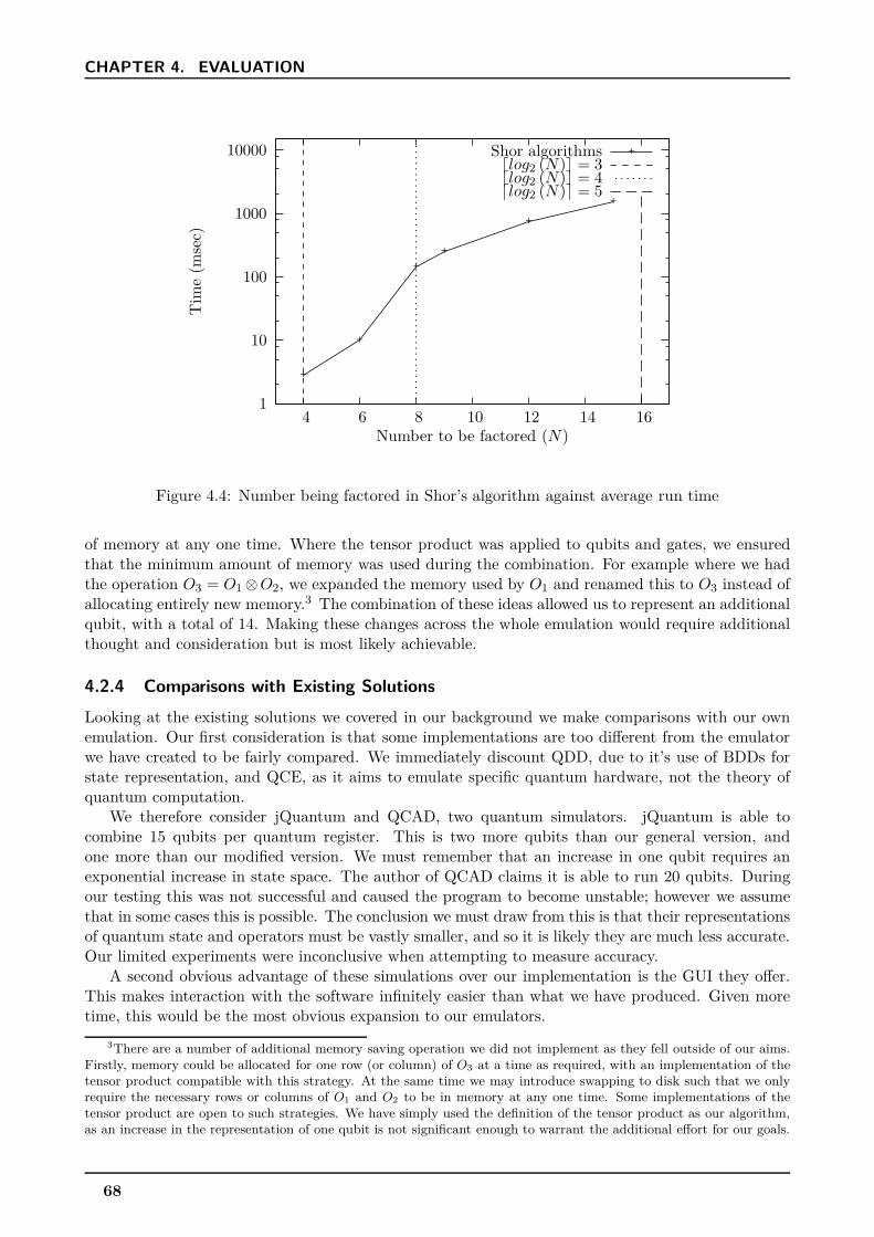
CHAPTER 4. EVALUATION
1
10
100
1000
10000
4 6 8 10 12 14 16
Tim
e(m
sec)
Number to be factored (N)
Shor algorithms
+
+
++
+
+
+dlog2 (N)e = 3dlog2 (N)e = 4dlog2 (N)e = 5
Figure 4.4: Number being factored in Shor’s algorithm against average run time
of memory at any one time. Where the tensor product was applied to qubits and gates, we ensuredthat the minimum amount of memory was used during the combination. For example where we hadthe operation O3 = O1 ⊗O2, we expanded the memory used by O1 and renamed this to O3 instead ofallocating entirely new memory.3 The combination of these ideas allowed us to represent an additionalqubit, with a total of 14. Making these changes across the whole emulation would require additionalthought and consideration but is most likely achievable.
4.2.4 Comparisons with Existing Solutions
Looking at the existing solutions we covered in our background we make comparisons with our ownemulation. Our first consideration is that some implementations are too different from the emulatorwe have created to be fairly compared. We immediately discount QDD, due to it’s use of BDDs forstate representation, and QCE, as it aims to emulate specific quantum hardware, not the theory ofquantum computation.
We therefore consider jQuantum and QCAD, two quantum simulators. jQuantum is able tocombine 15 qubits per quantum register. This is two more qubits than our general version, andone more than our modified version. We must remember that an increase in one qubit requires anexponential increase in state space. The author of QCAD claims it is able to run 20 qubits. Duringour testing this was not successful and caused the program to become unstable; however we assumethat in some cases this is possible. The conclusion we must draw from this is that their representationsof quantum state and operators must be vastly smaller, and so it is likely they are much less accurate.Our limited experiments were inconclusive when attempting to measure accuracy.
A second obvious advantage of these simulations over our implementation is the GUI they offer.This makes interaction with the software infinitely easier than what we have produced. Given moretime, this would be the most obvious expansion to our emulators.
3There are a number of additional memory saving operation we did not implement as they fell outside of our aims.Firstly, memory could be allocated for one row (or column) of O3 at a time as required, with an implementation of thetensor product compatible with this strategy. At the same time we may introduce swapping to disk such that we onlyrequire the necessary rows or columns of O1 and O2 to be in memory at any one time. Some implementations of thetensor product are open to such strategies. We have simply used the definition of the tensor product as our algorithm,as an increase in the representation of one qubit is not significant enough to warrant the additional effort for our goals.
68

4.2. THE QUANTUM CIRCUIT MODEL
The run times of algorithms in these simulations were comparable with what we achieved. In somecases they were slower, but this may be due to the overheads associated with a GUI.
In conclusion, our implementation is not massively behind these two simulations in terms ofperforming quantum computation, although an increase in our maximum state space size would bebeneficial. We must remember that our emulator performs greater amounts of computation thanthese simulations, so greater resource requirements are reasonable.
4.2.5 Limitations
Despite generally meeting the aims set out for the emulation, it does have a number of weaknesses.On top of the limitations in accuracy, efficiency, and the other points discussed above we outline moregeneral points here.
• We have not proved the correctness of our implementation. As mentioned, to even attempt todo so is extremely difficult, and there are limitless other cases we have not shown. Due to theimperfect nature of our classical representation, we will most likely never be able to prove itscorrectness, and only an approximate correctness. If we aimed to prove the correctness of analgorithm, for example, this would be a more achievable goal.
• We have shown that we are able to represent states accurately enough to correctly emulate thequantum algorithms we present in this report. Although we do not see any examples in theliterature for which this is the case, for more complex circuits this level of accuracy may not besuitable; we may have hundreds of operations performed between measurements.
• The gates we make available for use in circuits are limited. We are able to approximatelyrepresent any quantum gate as we have several universal sets of gates amongst those available.We would be able to resolve this limitation by implementing a parametrised universal gate, suchas J (α) presented in 3.5.1.
• We performed our evaluation using Cygwin on a Windows machine. Cygwin in particularis notoriously slow, and so our benchmarks are likely to be significantly slower than on anequivalent machine running Linux for example. We used this computer as it was the developmentmachine and most testing had occurred on it.
• One of the biggest drawbacks of the emulator we have developed is that it requires goodknowledge of the system to make good use of it. We have not provided a graphical user interfaceor implemented a formal input language (although we have developed a circuit calculus), andall circuits must be developed in code using the gate library and qubit functions.
• Our introduction clearly stated we are aiming to achieve a quantum emulation. With theinherent inaccuracies of the classical representation of quantum states, we will never achieve aperfect emulation in terms of accuracy. We are attempting to represent analogue systems usinglimited precision floating point numbers. We aim to imitate the function of a quantum system,which we have achieved, but for any input we can only provide an approximation (although avery accurate approximation) of the intermediate states. After measurement, our state resolvesto |0〉 or |1〉, so these inaccuracies are no longer present. Stricter definitions of emulation thanour own (see 1.2) could not be applied to our implementation.
4.2.6 Quantum Circuit Calculus
Our circuit calculus is able to represent any conventional circuit model diagram. We are able totranslate our calculus into a diagram, and also a diagram into our calculus. Our presentation of thecalculus is brief, and we only give a rough idea of its semantics; however it is suitable for our purpose.
We see two shortcomings of the calculus. We have no direct way of representing the differencebetween a wire of a circuit diagram representing multiple qubits (/n) and the expanded form of thiswhere each qubit is shown as a separate wire. Although equivalent, we are unable to distinguish
69

CHAPTER 4. EVALUATION
between the different forms using our calculus. Although we have not presented any examples of itin this text, some literature uses two parallel wires (=) to represent a classical bit value as opposedto a quantum value. For example, a qubit invariably takes a classical value after a measurement inthe standard basis. Our calculus has no way of signifying a wire as containing a classical value.
A more significant factor to consider is that we have no way of specifying input or output qubits.We imply their presence through the use of wires; however, introducing qubits into the calculus wouldallow us to fully specify complete algorithms as opposed to circuits.
Further expansion of our discussion would include the demonstration of some common equivalencesusing the calculus (CX and CZ for example) and the development of a standard form and rewritingrules, as has been given for the measurement calculus in [11].
4.3 Measurement-Based Quantum Computation
Our second main aim was to develop an emulation of measurement-based quantum computationusing the one-way quantum computer architecture and making use of the measurement calculus. Weare interested in determining to what extent it is possible to efficiently emulate this on a classicalcomputer, and what we are limited by. Much of the intention behind the evaluation of the quantumcircuit model can equally be applied to our measurement-based implementation. As both emulationshave a similar basis, we will refer to the evaluation of the circuit model for some aspects.
We will look at the correctness of the implementation, the accuracy our emulation achieves, and weinvestigate the bounds of our solution in terms of entangled qubits we can represent. We successfullyemulated the Deutsch and Deutsch-Jozsa algorithms; however we were unable to implement Shor’salgorithm due to its complexity. Without some form of minimisation we require more auxiliary qubitsthan with the circuit model, and so we were sooner restricted by memory than we would be with thecircuit model. Where possible, we do apply equivalent patterns requiring fewer qubits; however werequire more investigation into this area.
4.3.1 Demonstration of Correctness
We begin this section by showing the correctness of our implementation. For comparison, we willdemonstrate the same scenarios as for the circuit model. The structure of implementation is basedupon circuit model gates which we replace with equivalent patterns. As such, it is straightforward toimplement circuits in terms of the combinations of patterns representing gates.
Measuring a single qubit returns, probabilistically, the value with the highest probability of beingmeasured according to generalised measurement. We create patterns with which we are able togenerate the listed qubit states from classical inputs, upon which we perform measurements in thespecified basis. Our implementation adds the ability to make measurements in the standard basis(this is omitted from the measurement calculus) in order to provide direct comparison of our outputswith the circuit model.
The most fundamental part of MBQC is measurement, and we must be able to do this in the basis|+α〉, |−α〉 for any α ∈ [0, 2π]. We show some examples in Table 4.2, concentrating on measurementswith predictable outcomes for example purposes.
We see that each of the listed examples provides the same probabilities as we expect. We alsoconfirmed that each set of generated measurement matrices conforms to the requirement set out inEquation 3.23 in 3.4. We also observe that our qubits correctly collapse to the measured state.
Applying a pattern representing a quantum gate produces an output qubit with the state expected.Applying a pattern equivalent to sequentially combined patterns results in the same state asapplying each pattern individually, one after the other. Patterns were applied to a qubit with thegiven state. For the sequentially combined pattern IX ZH, if each pattern was applied individually,
70

4.3. MEASUREMENT-BASED QUANTUM COMPUTATION
Qubit state Basis Expected probability of Actual probability
measuring 1 (|1〉 or |−α〉) of measuring 1
|0〉 =[
1 0]T
|0〉, |1〉 0 0
|1〉 =[
0 1]T
|0〉, |1〉 1 1
|+0〉 = 1√2
[
1 1]T
|0〉, |1〉 0.5 0.5
|+0〉 |+0〉, |−0〉 0 0
|+π〉 = 1√2
[
1 −1]T
|+0〉, |−0〉 1 1
|+π〉 |+π〉, |−π〉 0 0
|ψ〉 = 12
[ √3 −i
]T|0〉, |1〉 0.25 0.25
|ψ〉 |+0〉, |−0〉 0.5 0.5
|ψ〉 |+π〉, |−π〉 0.5 0.5
|ψ〉 |+ π2〉, |− π
2〉 1
4
(
2 −√
3)
0.9330
Table 4.2: Measurement of single qubits
the qubit state for the intermediate steps are those stated in the rows above. We do not measure theoutput qubits in these examples. We use the definition of |ψ〉 given in the table above.
Our results (Table 4.3) show that we have successfully applied the patterns to our input qubits,resulting in the correct qubit state of the output qubit. We must note that the resultant state fromthe bottom two tests are of dimension 4, meaning they involve 2 qubits. We have separated the output(second) qubits in both cases by removing the first qubit, so we can clearly see the result we expect.
The parallel combination of qubits and patterns follow the laws of the tensor product. Whencombining qubit states or patterns together we ensure we have matrices of the correct dimension, andthe ordering of combinations are correct.
71

CHAPTER 4. EVALUATION
Input qubit state Pattern applied Expected output state Actual output state
|ψ〉 I := ({1} , {1} , {1} , ∅) |ψ〉[
0.8660
−0.5i
]
|ψ〉 X :=({1} , {1} , {1} ,X1
1
)
12
[
−i√3
] [
−0.5i
0.8660
]
12
[
−i√3
]
X :=({1} , {1} , {1} , Z1
1
) 12
[
−i−
√3
] [
−0.5i
−0.8660
]
12
[
−i−
√3
]
H := 12√
2
[
−√
3 − i√3 − i
] [
−0.6124 − 0.3535i
0.6124 − 0.3535i
]
({1, 2} , {1} , {2} ,Xs1
2 M01E1,2
)
|ψ〉 IX ZH := 12√
2
[
−√
3 − i√3 − i
] [
−0.6124 − 0.3535i
0.6124 − 0.3535i
]
({1, 2} , {1} , {2} ,Xs1
2 M01E1,2Z
11X
11
)
Table 4.3: Application of patterns
Qubit/gate combination Expected qubit state/gate Actual qubit state/gate
|+〉 ⊗ |−〉 12
[
1 −1 1 −1]T [
0.5 −0.5 0.5 −0.5]T
|ψ〉 ⊗ |ψ〉 14
[
3 i√
3 i√
3 −1]T [
0.75 0.4330i 0.4330i −0.25]T
H ⊗ I ({1, 2, 3}, {1, 3}, {2, 3} ,Xs1
2 M01E1,2
)
CX ⊗ X ({1, 2, 3, 4, 5}, {1, 5}, {1, 4, 5} ,X15Z
s3
4 Zs2
4 Zs2
1 M03M
02E1,2,3,4
)
We see that our resulting states and patterns are of the correct size and have the expected numberof input and output qubits. We confirm the same for multiple qubits and for large patterns, but donot show the resulting matrices and commands here due to their size.
We look at the Deutsch algorithm. By implementing a quantum algorithm we can ensure thatthe system is functioning correctly. We have the additional work of moving it from a circuit modelrepresentation to the relevant measurement calculus representation, but we have shown this in theprevious chapter to be
(
{1, 2, 3, 4, 5, 6, 7} , {1, 2} , {6, 7} ,Xs5
6 M05E5,6X
s4
7 M04E4,7X
s3
4 M−π3 E3,4X
s2
3 M02E2,3X
s1
5 M01E1,5
)
(4.1)
for the function f2. For the circuit model we were able to show the intermediate qubit states betweenthe application of each set of gates. For the measurement-based model, to show each step wouldtake many pages and so is not given here. The computation of states branches at each measurement,resulting in 32 different cases by the end of this pattern.
72

4.3. MEASUREMENT-BASED QUANTUM COMPUTATION
We confirm that for all functions f we successfully determine whether it is constant or balancedby returning a 0 or 1 respectively.
We look at the Deutsch-Jozsa algorithm. We have similar trouble evaluating the intermediatestates of the Deutsch-Jozsa algorithm. We allow the emulator to generate the combined patterns forn = 2, n = 3 and n = 4 and test that every value of fx returns the correct result for the algorithm.
Our difficulty here stems from the lack of intuition we have for measurement-based computation.Calculations of intermediate qubit states are not simple operations, and so confirming our results arecorrect requires the generation of every possible branch for every measurement possibility. Such a taskrequires automation, so to test intermediate states we require another simulator for comparison or atest harness. Instead, we make the assumption that if for every possible input we measure our outputqubits and they collapse to the correct state with a probability of 1 (therefore deterministically), wehave implemented the algorithm and our emulator correctly.
4.3.2 Accuracy
With the belief that our emulation is correct, we now quantify the accuracy of our implementation.Working with measurements in the basis |+α〉, |−α〉 means we are likely to generate far more roundingerrors than in the circuit model. This is due to two factors: we work with irrational numbers, andnumbers requiring long decimal representations, and measurement in non-standard bases uses andgenerates long decimal representations.
We do not look at the accuracy with which probabilistic behaviour is emulated. We cover this inthe previous section and use the same methods and technique to apply randomisation to probabilisticselection in both emulators.
Investigating the effects of different datatypes upon the accuracy of emulation versus the relativememory requirements. We cover the memory required for different datatypes in the previous sectionand refer to these figures where necessary. Our aim is to produce a similar investigation to determineif behaviour is the same with an equivalent measurement-based test.
Again, we have trouble evaluating our measurement-based model. If we aim to implement a seriesof H patterns we have the problem that each requires an auxiliary qubit each, and so our state spacegrows with each application. Applying 11 H patterns in series requires 12 entangled qubits (so a statespace of dimension 212 = 4096) and takes a number of minutes to complete. What we see is at firstslightly alarming.
We see no rounding error for the float, double or long double datatypes. The only inaccuracywe see is from the representation error that exists wherever an irrational or long number is stored asa finite floating point number.
After some consideration, we realise that after each measurement (which occurs every 3 operatorsin our H pattern) we collapse to a definite state. For this example we collapse to the state |+0〉 or|−0〉. We calculate these collapse states from scratch every time we make a measurement. Any errorpresent in the state space is eradicated when we take the measurement, and it only (minutely) affectsthe probability of measuring either state.
With this significant finding we can reduce our floating point representation to something smallerwith no consequential loss of accuracy.
4.3.3 Efficiency and Bounds
Determining the efficiency and bounds of our emulation will be a key aspect in the comparison of ourtwo emulations. We did not develop our implementation with the aim of maximising either efficiency(run time and resource usage), or the bounds (number of qubits), but we investigate what we haveachieved.
73

CHAPTER 4. EVALUATION
By converting patterns to a standard form we are able to predict the pattern of entanglement andmeasurement, and so predict the required resources from the number of qubits, entanglements andmeasurements.
Algorithm running times. The most obvious measure of our implementation is to see how long ittakes to run each quantum algorithm. We repeat each algorithm 1,000,000 times on five occasionsfor the shorter algorithms, taking the average. For the longer running algorithms we reduce this to100,000 or 10,000 repetitions. Where an algorithm can be given different inputs, we equally alternatebetween all possible (valid) inputs.
Algorithm Average run time (ms) Algorithm Average run time (ms)
Deutsch / D-J, n = 1 86.76 D-J, n = 6 683.4
Deutsch-Jozsa, n = 2 182.2 D-J, n = 7 857.0
Deutsch-Jozsa, n = 3 284.6 D-J, n = 8 1006
Deutsch-Jozsa, n = 4 404.3 D-J, n = 9 1253
Deutsch-Jozsa, n = 5 523.0 D-J, n = 10 1713
We expect the time taken for increasing values of n to steadily but exponentially increase. Theincrease will be much slower than for the circuit model. This is because our I and X patterns, whichwe use to create our Uf operators, do not increase the size of the quantum state space. These patternsare combined using the tensor product, meaning we effectively develop n + 1 parallel, independentcircuits. As a result we have n+ 1 different quantum registers, each with a similar number of qubitsin each. This means our quantum state spaces remain relatively small in comparison to the overallnumber of qubits, and so we see our run times do not increase exponentially as they did with thecircuit model.
We plot the graph of these results showing the number of qubits against average run time (Figure4.5). Within the results we have a steady exponential increase, as we predicted, but we also seefluctuations; our line is not straight. We can put this down to the competing effects of increasingqubit state spaces and increasing algorithmic complexity for generating and combining patterns, actingagainst an increase in the number of qubit registers (groups of entangled qubits) we have.
Investigate the number of qubits we can represent and perform commands upon. We look atthe maximum number of qubits we can entangle together. We are not particularly interested in thespecific pattern with which we test the bounds, and so we develop a simple test pattern:
T := ({1, 2, . . . , n} , {1} , {n} , E1,2,...,n) . (4.2)
We are able to process this pattern for all values of n up to and including n = 13. Whenattempting to emulate n = 14 we receive an error relating to the allocation of memory, implyingwe have utilised all memory available on the test machine. Monitoring resource usage confirms anexhaustion of available memory and supports this idea. In our introduction we mention that memoryis the bounding factor of classical implementations of quantum systems, and we have confirmed thisin our investigation.
74

4.3. MEASUREMENT-BASED QUANTUM COMPUTATION
10
100
1000
10000
0 2 4 6 8 10 12
Tim
e(m
sec)
Number of qubits (n+ 1)
D-J algorithms
+
+
++
++
+ ++
+
+
Figure 4.5: Number of qubits in the Deutsch-Jozsa algorithm against average run time
4.3.4 Limitations
Our emulation or MBQC was not as successful as that of the circuit model. This is due to a numberof factors:
• There is far less literature available on the subject, and much of it is focused on the physicalimplementation aspect.
• No simulation of MBQC has been attempted before so everything we develop is new.
• The complexity of the algorithms required to perform four way entanglement, measurements innon-standard bases, and to manage dependent commands is much greater than any part of thecircuit model. With the circuit model we have clear linear steps, whereas in MBQC we mustconsider many factors at any one time. To create the same kind of flexibility that the circuitmodel offers requires much more thought and development time. Due to limitations on time wewere unable to develop our implementation as much as we hoped, and ultimately the complexityof Shor’s algorithm meant we were unable to implement it other than at a very basic level.
• We do not exploit the full level of standardisation and minimisation discussed in our theory. Weinclude a number of possible improvements in the following chapter.
• It is extremely difficult to develop an intuition for the measurement-based model, largely asit has no classical analogue. Developing an arbitrary pattern to solve a specific goal requiresa significant amount of thought. As such, we are very much tied to the circuit model andbase our implementation upon patterns which are equivalent to quantum gates. This resultsin patterns using more auxiliary qubits and commands than necessary, and means we mustcombine multiple patterns (representing gates) together to form circuits. If it they were fullyimplemented, minimisation and standardisation would help ease this problem by ensuring wedo not include unnecessary qubits or commands.
• We can implement any command sequence, and any pattern given that we have enough memoryto represent the state spaces. What we lack is the ability to specify patterns in a simple language.Currently we use constructors to specify arbitrary patterns or call pre-defined patterns. A simpleGUI would vastly improve the ease with which we can implement patterns.
75

CHAPTER 4. EVALUATION
0.01
0.1
1
10
100
1000
10000
100000
106
0 2 4 6 8 10 12 14
Tim
e(m
sec)
Number of qubits (n+ 1)
Circuit model
++
+
+
+
+
+
+
+
+
+
+
+Measurement-based
rsrs
rs rs rs rs rs rs rs rs
rs
Figure 4.6: Number of qubits in the Deutsch-Jozsa algorithm against average run time
4.4 Comparisons Between Models
With an implementation and evaluation of both approaches, we make some comparisons between thetwo. These comparisons are made under very specific scenarios, and as such, it is likely to be difficultto draw any generalised conclusions with significant evidence. Even so, any comparison is useful forour purposes. Some additional discussion has been made during our description of each of the models.
4.4.1 Efficiency, Bounds and Accuracy
We use the time taken to run the Deutsch-Jozsa algorithm for different values of n as our benchmarkof efficiency. To most easily make a comparison between models we plot results for both models(Figure 4.6).
From this we see that although the circuit model begins far in the lead, its timings increase pastthe run time of the MBQC between 10 and 11 qubits. This is a very interesting observation. It seemsthat the measurement model copes better with larger numbers of qubits, whereas the circuit modelexhibits the state explosion problem. Our investigation led us to discover that our MBQC modelwas creating n+ 1 parallel, independent circuits which reduces the maximum size of state spaces andimproves the efficiency of computation.
It may be that we only see this behaviour from MBQC in this specific scenario as state spacesare kept separate, but this may also be down to an advantage of the approach. The next step toanalysing this comparison further is to create other equivalent circuits with changeable numbers ofcombined qubits and repeat the experiment.
Our bounds, defined in terms of the number of combined qubits we can represent, are similar forboth models. For the circuit model we see the general case of 13 qubits; however we some modificationswe can increase this to 14. For MBQC we also have 13 qubits generally. We put this similarity downto the almost identical qubit state representations we have. This points to the state representationas an obvious bottle neck which we should concentrate upon improving in future development.
Finally, we compare the accuracy of both models. With the circuit model we describe a high levelof accuracy and see that rounding errors would only have an effect after hundreds of gate applications.With MBQC we discovered an extremely interesting property. We saw that due to the frequency of
76

4.4. COMPARISONS BETWEEN MODELS
measurements (generally within 3 operations), rounding errors had no time to build up. Where wehave patterns in standard form we apply all of our measurements together, followed by corrections.As the only corrections we apply are X and Y , which are both integer operators, rounding errors donot appear in this case either.
4.4.2 Equivalence & Conversion between Models
Our MBQC emulator is based upon much of the theory we developed for the circuit model. Thisincludes the representation of qubits and corrections we use, as well as the way in which patternscombine to form a circuit. On top of this, we use measurement patterns that are equivalent to quantumgates in order to create circuits. The normal generation of patterns and circuits is equivalent to thecircuit model.
Assuming our emulators both function correctly, implementing a circuit for the circuit model,and then combining the equivalent patterns of the circuit’s component gates in the same way shouldproduce identical outputs given the same input. As such, where we prove an algorithm or desirethe behaviour of a specific circuit, we can equally show the same for the MBQC model when usingequivalent patterns.
We have not demonstrated or investigated an equivalence of MBQC patterns for the circuit model.Beginning with the standard form of patterns, this may be an interesting line of investigation. Wewould likely find that some sequence of commands can be implemented with a unitary gate U .
Ultimately, whichever model we prefer for computation, given equivalences between models, weshould be able to achieve the same computational result for any model. It is obvious from ourinvestigations that developing an algorithm for the circuit model is infinitely easier than developing oneusing MBQC directly. However, MBQC may prove the most computationally effective, both physicallyand when emulating. We can then use equivalences to convert our new algorithm to MBQC, performstandardisation and minimisation of the pattern, and have the advantages of improved performance.
77


Chapter 5
Conclusions
At any rate, it seems that the laws of physics present no barrier to reducing the sizeof computers until bits are the size of atoms, and quantum behaviour holds sway.
Richard P. Feynman [25]
5.1 Introduction
To conclude this thesis we summarise what we have achieved, both in terms of deliverables and interms of learning. We present three major contributions:
• An expansive and detailed summary of the theory of quantum computation, including the relatedmathematics and quantum mechanics.
• A circuit-based quantum computation emulator with which we implemented the Deutsch, Deutsch-Jozsa and Shor algorithms.
• We have developed the first measurement-based quantum computation emulator. We implementthe Deutsch and Deutsch-Jozsa algorithms using patterns equivalent to quantum circuit gates.We were unable to implement Shor’s algorithm due to the complexity of the problem.
The two emulators are the product of developing a sound understanding of the theory of quantumcomputation which is presented throughout the report. Ultimately we are able to accurately emulatequantum computation with up to 13 entangled qubits for both approaches. Our emulations arerelatively fast and are flexible with respect to what circuits and patterns can be implemented withthem.
In our evaluation we demonstrated the effects of the state explosion problem which prevented usfrom combining more than 13 qubits together. Our experimental results confirmed the hypothesisthat memory would be our bounding factor for state representation.
While developing our MBQC theory we discovered that when measuring in the non-standard basespresented in the measurement calculus we cannot use von Neumann measurement for all values of α.We instead used generalised measurement (POVM).
The high accuracy of our qubit state space representations was unnecessary for our purposes,and investigations revealed that measurements removed any rounding errors. A decreased level ofaccuracy would allow a greater number of combined qubits to be emulated.
In our evaluation we present benchmarks for the algorithms we have implemented. For the circuitmodel a run of Shor for N = 15 takes 1.5 seconds. Our emulation fairs well against existing solutionsin this regard; however falls down due to the relatively small number of qubits that can be represented.
In our final section we consider a number of expansions to the project that could be considered inthe future.
79

CHAPTER 5. CONCLUSIONS
5.2 Future Work
We present a number of expansions to this project that we could investigate given more time. Wefirst discuss methods of increasing the bounds of our implementation:
• There are two significant lines of investigation for increasing the bounds of emulation. The first isto increase the memory available on a single computer, for example using a super computer. Thesecond is to distribute the implementation across many machines. Altering our system to utilisea super computer is a relatively straightforward task. Simply running our existing emulatorswith the additional resources offered by such a computer would see an immediate increase inbounds. From this we can make additional improvements such as threading computation sothat we are able to utilise many CPU cores.
• Distributing the emulators we have developed is a difficult task. We must rethink the entire sys-tem and develop an implementation that is parallelisible and efficiently handles the distributionof resources (CPU and memory). We must also ensure that network communication does notslow down computation to the extent that any significant advantage of distribution is lost. Forexample, we should investigate the use of compression when sending large amounts of data. MPI(Message Passing Interface) would be the obvious distribution framework to use here. Targetingthe use of regular workstation computers as opposed to high performance computers would bean advantageous approach and more readily usable by others.
• If we force operators and states to be written to the hard drive when memory becomes low,we only require enough physical memory to store one row and column of a state or operator inorder to complete numerical operations. This would greatly slow down the run time but shouldvastly increase the limit of qubit representations. There are many algorithms that are able toperform these kinds of operations in an efficient manner to maximise the available resources.
• Our evaluation shows that our implementations are very accurate, but at the same time weuse a significant amount of additional memory in order to achieve this. Reducing our aims foraccuracy would allow us to decrease representation size, and therefore emulate more qubits withthe same amount of memory.
We consider ways in which our deliverables could be made more useful and usable to potential users:
• We had no specific users in mind when developing the emulators, and as such, it became aspecialised system requiring a good knowledge of its construction in order to use it. The mostdesirable solution would be a inclusive, polished, GUI based, end product. For the circuit model,we would allow the input of a circuit via the circuit calculus or via a circuit builder interface.For the measurement model, input would be via the measurement calculus. A similar builderfor measurement patterns may be developed; however it is an unintuitive process and may provetoo difficult to use. The output of quantum states and measurements should be in a number offorms such that the user can decide which is most meaningful to them for their purposes. Weshould be able to view any intermediate steps of computation; for example, the state of qubitsbetween gates.
• Following on from the previous idea, outputting the intermediate steps of computation as aseparate file, such as an image, text or LATEX would be useful for those wishing to understand acircuit. If this output was made human readable using surds, fractions and irrational numberssuch as π, it would make working theoretically with algorithms much easier.
• An initial idea of this project was to incorporate teaching into the tool such that undergraduatestudents would be able to learn about quantum systems and quantum computation. Thesimulation of the two models followed as a part of this concept. Now that we have developedemulators, the addition of a teaching element to the tool would provide a useful introductionand explain the specifics of the tool while introducing the quantum topics.
80

5.2. FUTURE WORK
• There is huge scope for further developing our circuit calculus. We have introduced the syntaxand semantics of the calculus, but as we see from the measurement calculus, there is wide rangeof discussion that can result from it. An obvious expansion which we mention below is thetranslation between our circuit calculus and the measurement calculus. In our evaluation wemention two scenarios we do not account for. Specifically the specification of wires representingmultiple qubits, and wires representing classical bits. Adding these features would enhance theflexibility of the calculus. In addition, the expansion to include input and output qubits inour calculus would allow us to specify complete quantum algorithms instead of circuits. Asmentioned throughout this report, it is very difficult to develop intuition for MBQC. More so,we see circuit representations of measurement-based patterns in the literature. To expand ourcalculus to cover these cases would involve being able to specify the basis of measurements,linking dependent operators to the measurement upon which they depend, and allowing thearbitrary selection of control and target qubits in controlled gates.
Our final ideas for future investigation are into new theoretical areas:
• We have mentioned another measurement-based quantum computation approach called tele-portation. An obvious expansion to what we have covered is to create an emulator for thisarchitecture in a similar way to the emulators presented here. There are a number of otherapproaches to quantum computation which could be investigated in a similar way.
• Our MBQC emulator makes significant use of equivalences between quantum gates and measurement,and as such there is some implied conversion between models. Developing a full, two-waytranslation between models would be a significant achievement. This would likely be specifiedformally between calculi such as the circuit calculus we develop and the measurement calculus.From here the translation can be expanded to new approaches and we are then able to easilyimplement circuits and algorithms on any architecture.
• This idea leads onto a more detailed investigation into the comparisons between different modelsof computation. In our evaluation we have presented a brief and largely superficial look at thecircuit and measurement-based models; however there is huge area for expansion in order todraw more generalised conclusions. Ultimately, successful model will be chosen based uponwhich lends itself best to physical implementation.
• We mention in 3.7.2 that we should be able to develop a series of rewrite rules in order tominimise sequences of commands and thus reduce the number of qubits a pattern requires. Thisis an interesting area to investigate as this will have application not only in our emulation, butalso in real world implementations.
81


Bibliography
[1] D. Abbott, C. R. Doering, C. M. Caves, D. M. Lidar, H. E. Brandt, A. R. Hamilton, D. K. Ferry,J. Gea-Banacloche, S. M. Bezrukov, and L. B. Kish. Dreams Versus Reality: Plenary DebateSession on Quantum Computing. Quantum Information Processing, 2(6):449–472, December2003. doi: 10.1023/B:QINP.0000042203.24782.9a.
[2] D. Aharonov. Quantum Computation. In D. Stauffer, editor, Annual Reviewsof Computational Physics, volume VI. World Scientific, December 1998. URLhttp://arxiv.org/abs/quant-ph/9812037v1.
[3] P. Aliferis and D. W. Leung. Computation by measurements: a unifying picture. Physical ReviewA, 70(6), December 2004. doi: 10.1103/PhysRevA.70.062314.
[4] Amazon Inc. Amazon Elastic Compute Cloud (Amazon EC2), 2008. URLhttp://aws.amazon.com/ec2/.
[5] D. P. Anderson, J. Cobb, E. Korpela, M. Lebofsky, and D. Werthimer. SETI@home: Anexperiment in public-resource computing. Communications of the ACM, 45(11):56–61, November2002. doi: 10.1145/581571.581573.
[6] J. Bak and D. J. Newman. Complex Analysis. Springer, 2nd edition, 1996. ISBN 0387947566.
[7] A. L. Beberg, D. L. Ensign, G. Jayachandran, S. Khaliq, and V. S. Pande. Folding@home: Lessonsfrom eight years of volunteer distributed computing. In IPDPS ’09: Proceedings of the 2009 IEEEInternational Symposium on Parallel & Distributed Processing, pages 1–8, Washington, DC, USA,2009. IEEE Computer Society. ISBN 9781424437511. doi: 10.1109/IPDPS.2009.5160922.
[8] G. Brassard. Searching a Quantum Phone Book. Science, 275(5300):627–628, January 1997. doi:10.1126/science.275.5300.627.
[9] I. Chuang. Quantum circuit viewer: qasm2circ, March 2005. URLhttp://www.media.mit.edu/quanta/qasm2circ/.
[10] V. Danos, E. Kashefi, and P. Panangaden. The Measurement Calculus. Journal of the ACM, 54(2), April 2007. doi: 10.1145/1219092.1219096.
[11] V. Danos, E. Kashefi, P. Panangaden, and S. Perdrix. Extended Measurement Calculus. InS. Gay and I. Mackie, editors, Semantic Techniques for Quantum Computation, chapter 7, pages235–310. Cambridge University Press, New York, 2010. ISBN 052151374.
[12] B. Dawes and D. Abrahams. Boost C++ Libraries. URL http://www.boost.org/.
[13] A. de Vries. jQuantum: Quantum Computer Simulator, March 2010.
[14] D. Deutsch. Quantum Theory, the Church-Turing Principle and the Universal QuantumComputer. Proceedings of the Royal Society of London. A. Mathematical and Physical Sciences,400(1818):97–117, July 1985. doi: 10.1098/rspa.1985.0070.
83

BIBLIOGRAPHY
[15] D. Deutsch. Quantum Computational Networks. Royal Society of London Proceedings Series A,425:73–90, September 1989.
[16] D. Deutsch. The Fabric of Reality: The Science of Parallel Universes and Its Implications.Penguin Books, 1997. ISBN 014027541X.
[17] D. Deutsch and R. Jozsa. Rapid solution of problems by quantum computation. Proceedings ofthe Royal Society of London, Series A, 439:553–558, October 1992.
[18] P. A. M. Dirac. The Principles of Quantum Mechanics (International Series of Monographs onPhysics). Oxford University Press, USA, 4th edition, February 1982. ISBN 0198520115.
[19] D. P. DiVincenzo. Quantum Computation. Science, 270(5234):255–261, October 1995. doi:10.1126/science.270.5234.255.
[20] D. P. DiVincenzo. Two-bit gates are universal for quantum computation. Physical Review A, 51(2):1015–1022, February 1995. doi: 10.1103/PhysRevA.51.1015.
[21] D. P. DiVincenzo. Solid State Quantum Computing, 2000. URLhttp://www.research.ibm.com/ss_computing/.
[22] D. P. DiVincenzo. The Physical Implementation of Quantum Computation. Fortschritte derPhysik, H.-L., 2000. URL http://arxiv.org/abs/quant-ph/0002077. Experimental Proposalsfor Quantum Computation.
[23] A. Edalat. Notes from the course 484: Quantum Computing. Departmentof Computing Imperial College London, 2009. Imperial College London. URLhttp://www.doc.ic.ac.uk/~ae/teaching.html#quantum.
[24] A. Ekert, P. Hayden, and H. Inamori. Basic concepts in quantum computation. November 2000.URL http://arxiv.org/abs/quant-ph/0011013v1.
[25] R. P. Feynman. Simulating Physics with Computers. International Journal of Theoretical Physics,21(6):467–488, June 1982. doi: 10.1007/BF02650179.
[26] R. P. Feynman. Quantum mechanical computers. Foundations of Physics, 16(6):507–531, June1986. doi: 10.1007/BF01886518.
[27] C. Fox. QCF: Quantum Computing Functions for MATLAB. Technical Report PARG-03-02, Pattern Analysis & Machine Learning Research Group, University of Oxford, 2003. URLhttp://www.robots.ox.ac.uk/~parg/pubs/qcf.pdf.
[28] E. Gabriel, G. E. Fagg, G. Bosilca, T. Angskun, J. J. Dongarra, J. M. Squyres, V. Sahay,P. Kambadur, B. Barrett, A. Lumsdaine, R. H. Castain, D. J. Daniel, R. L. Graham, and T. S.Woodall. Open MPI: Goals, Concept, and Design of a Next Generation MPI Implementation. InProceedings, 11th European PVM/MPI Users’ Group Meeting, pages 97–104, Budapest, Hungary,September 2004. URL http://www.open-mpi.org/.
[29] J. Gilbert and L. Gilbert. Linear Algebra and Matrix Theory. Brooks Cole, 2nd edition, 2004.ISBN 0534405819.
[30] D. T. Gillespie. A quantum mechanics primer: An Elementary Introduction to the Formal Theoryof Non-relativistic Quantum Mechanics. John Wiley & Sons, New York, 1974. ISBN 0470299126.
[31] D. Gottesman and I. Chuang. Demonstrating the viability of universal quantum computationusing teleportation and single-qubit operations. November, 402(6760):390–393, November 1999.doi: 10.1038/46503.
84

BIBLIOGRAPHY
[32] D. Greve. Qdd - a quantum computer emulation library, September 2007.
[33] L. K. Grover. A fast quantum mechanical algorithm for database search. In STOC ’96:Proceedings of the twenty-eighth annual ACM symposium on Theory of computing, pages 212–219,New York, NY, USA, 1996. ACM Press.
[34] L. K. Grover. Quantum Mechanics helps in searching for a needle in a haystack. Physical ReviewLetters, 79(2):325–328, July 1997. doi: 10.1103/PhysRevLett.79.325.
[35] D. Hanneke, J. P. Home, J. D. Jost, J. M. Amini, D. Leibfried, and D. J. Wineland. Realizationof a programmable two-qubit quantum processor. Nature Physics, 6:13–16, November 2009. doi:10.1038/nphys-1453.
[36] M. Hayward. Quantum Computing and Shor’s Algorithm. April 2008. URLhttp://alumni.imsa.edu/~matth/quant/299/paper.pdf.
[37] R. Jozsa. An introduction to measurement based quantum computation. In D. G. Angelakis,editor, Quantum Information Processing: from theory to experiment, chapter 2, pages 137–158.IOS Press Inc., 2006. URL http://arxiv.org/abs/quant-ph/0508124.
[38] P. Kaye, R. Laflamme, and M. Mosca. An introduction to quantum computing. Oxford UniversityPress, 1st edition, November 2006. ISBN 019857049X.
[39] D. W. Leung. Quantum computation by measurements. International Journal of QuantumInformation, 2(1):33–43, March 2004. doi: 10.1142/S0219749904000055.
[40] S. Lloyd. Universal Quantum Simulators. Science, 273(5278):1073–1078, August 1996. doi:10.1126/science.273.5278.1073.
[41] K. Michielsen and H. de Raedt. QCE: A Simulator for Quantum Computer Hardware, August2003. URL http://rugth30.phys.rug.nl/compphys0/qce.htm.
[42] G. E. Moorhouse. Notes from the seminar: Shor’s Algorithm for Fac-torizing Large Integers. University of Wyoming, November 2000. URLhttp://www.uwyo.edu/moorhouse/slides/talk2.pdf.
[43] M. A. Nielsen. Quantum computation by measurement and quantum memory. Physics LettersA, 308(2-3):96–100, February 2003. doi: 10.1016/S0375-9601(02)01803-0.
[44] M. A. Nielsen. Optical quantum computation using cluster states. Physical Review Letters, 93(4), July 2004. doi: 10.1103/PhysRevLett.93.040503.
[45] M. A. Nielsen. Cluster-state quantum computation. Reports on Mathematical Physics, 57(1):147–161, February 2006. doi: 10.1016/S0034-4877(06)80014-5.
[46] M. A. Nielsen and I. L. Chuang. Quantum Computation and Quantum Information. CambridgeUniversity Press, 1st edition, October 2000. ISBN 0521635039.
[47] J. Niwa, K. Matsumoto, and H. Imai. General-purpose parallel simulator for quantum computing.Physical Review A, 66(6), December 2002. doi: 10.1103/PhysRevA.66.062317.
[48] A. Peres. Quantum Theory: Concepts and Methods. Springer, 1st edition, 1993. ISBN0792336321.
[49] Quantiki. List of Quantum Computation Simulators. URLhttp://www.quantiki.org/wiki/List_of_QC_simulators.
85

BIBLIOGRAPHY
[50] R. Raussendorf and H. J. Briegel. A One-Way Quantum Computer. Physical Review Letters, 86(22):5188–5191, May 2001. doi: 10.1103/PhysRevLett.86.5188.
[51] R. Raussendorf, D. E. Browne, and H. J. Briegel. Measurement-based quantum computationwith cluster states. Physical Review A, 68(2), Aug 2003. doi: 10.1103/PhysRevA.68.022312.
[52] B. S. Rubin. Our First Qubit Measurement, January 2009. URLhttp://bradrubin.com/Site/Blog/Entries/2009/1/3_Our_First_Qubit_Measurement.html.
[53] J. H. Scanlon and B. Wieners. The Internet Cloud, September 1999. URLhttp://www.thestandard.com/article/0,1902,5466,00.html.
[54] P. W. Shor. Algorithms for quantum computation: Discrete logarithms and factoring. InS. Goldwasser, editor, Proceedings of the 35th Annunl Symposium on the Foundations ofComputer Science, volume 35, pages 124–134, 1994.
[55] P. W. Shor. Polynomial-Time Algorithms for Prime Factorization and Discrete Logarithms ona Quantum Computer. SIAM Journal on Computing, 26(5):1484–1509, 1997. doi: 10.1137/S0097539795293172.
[56] J. Stolze and D. Suter. Quantum Computing: A Short Course from Theory to Experiment.Wiley-VCH, 2nd edition, 2008. ISBN 3527407871.
[57] S. Turgut. Notes from the course PHYS 737: Generalized Measurements. Departmentof Physics Middle East Technical University, 2007. Middle East Technical University. URLhttp://www.physics.metu.edu.tr/~sturgut/737/.
[58] M. Van den Nest, W. D"ur, G. Vidal, and H. J. Briegel. Classical simulation versus universality in measurement-basedquantum computation. Physical Review A, 75(1), January 2007. doi: 10.1103/PhysRevA.75.012337.
[59] L. Vandersypen, M. Steffen, G. Breyta, C. Yannoni, M. Sherwood, and I. Chuang. Experimentalrealization of Shor’s quantum factoring algorithm using nuclear magnetic resonance. Nature, 414(6866):883–887, 2001. doi: 10.1038/414883a.
[60] H. Watanabe. QCAD: GUI environment for Quantum Computer Simulator, September 2009.URL http://apollon.cc.u-tokyo.ac.jp/~watanabe/qcad/.
[61] N. S. Yanofsky. An Introduction to Quantum Computing. August 2007. URLhttp://arxiv.org/abs/0708.0261.
[62] N. S. Yanofsky and M. A. Mannucci. Quantum Computing for Computer Scientists. CambridgeUniversity Press, 1st edition, August 2008. ISBN 0521879965.
All web references accessed in May 2010.
86

Appendices
87


Appendix A
Related Mathematics
A.1 Introduction
An integral part of quantum mechanics is the understanding of complex numbers (A.3), and as such,it is an essential concept in quantum computing. Expanding on this, quantum theory relies heavilyupon the use of linear algebra; more specifically, complex vector spaces (A.6). Both complex numbersand linear algebra will be covered here to a depth necessary to understand the mathematics involvedin the project, with references to additional material. Those with a good understanding of thesetopics can begin at B and refer to previous sections where necessary. To highlight the unmistakableimportance of these topics, it has been said that “quantum theory is cast in the language of complexvector spaces” [62], so we will begin with this.
A.2 Imaginary Numbers
Imaginary numbers were introduced as part of the theory algebraic equations, in short, to solve theequation
x2 = −1. (A.1)
In order to do so we must postulate that such a number i (termed the imaginary unit) exists suchthat
i2 = −1 or i =√
−1. (A.2)
The set of imaginary numbers, I, is made up of multiples of i with a real number, such as 2 × i,3 × i, or n× i for any real number n.
A.3 Complex Numbers
Following on from this, a complex number, z, is a the composition of a real number and an imaginarynumber in the form
z = a+ bi, (A.3)
where a and b are termed the real and imaginary parts respectively and i denotes the imaginary unit.The set of complex numbers is denoted C, and with this it is possible to define both the sets of
real numbers, R, and imaginary numbers, I, as subsets of C. If the imaginary part of the complexnumber z is always taken as b = 0, the real number a is described by the complex number
z = a+ 0i = a. (A.4)
Conversely, if the real part of the complex number z is always taken as a = 0, the imaginarynumber b is described by the complex number
z = 0 + bi = bi. (A.5)
89

APPENDIX A. RELATED MATHEMATICS
A.4 Operations On Complex Numbers - C
To understand how we will work with complex numbers, we will outline the results of variousmathematical operations upon complex numbers c1 = a1 + b1 and c2 = a2 + b2. As the majorityof readers should be familiar with the topic, we will simply include definitions of each operation as areminder, and show worked examples where c1 = 2 + 3i and c2 = 17 + 5i.
A.4.1 Addition
c1 + c2 = (a1 + b1i) + (a2 + b2i) = (a1 + a2) + (b1 + b2)i
= (2 + 3i) + (17 + 5i) = (2 + 17) + (3 + 5)i = 19 + 8i (A.6)
A.4.2 Subtraction
c1 − c2 = (a1 + b1i) − (a2 + b2i) = (a1 − a2) + (b1 − b2)i
= (2 + 3i) − (17 + 5i) = (2 − 17) + (3 − 5)i = −15 − 2i (A.7)
A.4.3 Multiplication
c1 × c2 = (a1 + b1i) × (a2 + b2i) = (a1a2 − b1b2) + (a2b1 + a1b2)i
= (2 + 3i) × (17 + 5i) = (2 × 17 − 3 × 5) + (2 × 5 + 3 × 17)i = 19 + 61i (A.8)
A.4.4 Division
For division of complex numbers we must recall that division is defined as the inverse of multiplication,giving us
c1
c2=
a1 + b1i
a2 + b2i=a1a2 + b1b2
a22 + b2
2
+a2b1 − a1b2
a22 + b2
2
i
=2 + 3i
17 + 5i=
2 × 17 + 3 × 5
172 + 52+
17 × 3 − 2 × 5
172 + 52i =
60
314(A.9)
A.4.5 Conjugation
c = a+ bi, c = a− bi (A.10)
c1 = (2 + 3i) = 2 − 3i (A.11)
A.4.6 Modulus (Magnitude)
|c1| = |a+ bi| =√
a2 + b2
= |2 + 3i| =√
13 (A.12)
When describing the normalisation of a complex number c, we are referring to |c|2:
|c1|2 = c1 × c1
|2 + 3i|2 = (2 + 3i) × (2 − 3i)√
132
= (4 + 9) + (6 − 6)i = 13. (A.13)
It will become apparent how the normalisation of complex numbers is extremely important as wecome to manipulate quantum bits.
90

A.5. REPRESENTATION OF COMPLEX NUMBERS
Imaginary
Rea
l
2 + 3i
2
3
Figure A.1: Cartesian representation of complex number 2 + 3i
A.5 Representation of Complex Numbers
Beyond the algebraic applications of complex numbers, their significance is also apparent in geometry.With this, we see how it opens up the advantages of their use in physics.
A.5.1 Cartesian Representation
We can see in Figure A.1 how a complex number can be represented as a vector on the Argand plane(complex plane), with the axes determining the real and imaginary parts of the number.
Defining a complex number z as a pair of real numbers representing the real and imaginary parts,a and b respectively, of the complex number gives us
z 7−→ (a, b), (A.14)
the mapping of a complex number to the complex plane described. Effectively this provides us witha point in the Cartesian two-dimensional coordinate system. In our example it would give us
c1 7−→ (2, 3). (A.15)
As this effectively allows us to ignore the presence of i it is very useful and we will concentrate uponthis representation of complex numbers.
A.5.2 Polar Representation
We can also determine a complex number z from its modulus (magnitude) ρ and angle (phase) θ:
z 7−→ (ρ, θ). (A.16)
This form, as shown in Figure A.2, is described as the polar representation of complex numbers.The values of ρ and θ are computed from real and imaginary parts a and b by
ρ =√
a2 + b2 and θ = tan−1(
b
a
)
, (A.17)
or reversed usinga = ρ cos (θ) and b = ρ sin (θ) . (A.18)
Our example gives
c1 7−→(√
4 + 9, tan−1(
3
2
))
=(√
13, 0.983)
. (A.19)
91

APPENDIX A. RELATED MATHEMATICS
Imaginary
Rea
l
2 + 3i
0.983
√ 13
Figure A.2: Polar representation of complex number 2 + 3i
Considering the geometry of complex numbers, we can perform many of the operations describedpreviously (A.4) through geometric transformations or techniques. We will not cover this here;however any textbook on linear algebra would cover this topic.
A.6 Complex Vector Spaces
Taking complex numbers a step further, we will provide a very brief introduction to the vast subjectof complex vector spaces. Our motive for covering this topic is that the state of a quantum systemcorresponds to a vector in a complex vector space. We will use vectors to describe states and matrices,covered later (A.8), as a way to describe dynamics.
In computing terms, a vector can be considered to be a one-dimensional array. For the majorityof our examples we shall use the n-dimensional complex vector space C
n. This vector space includesall vectors of some fixed dimension containing complex numbers. The specific case we will begin withis an ordered set of dimension 6, denoted C
6 = C × C × C × C × C × C, with an example of such acomplex vector represented as
V =
2 + 3i
17 + 5i
3 − 2i
11 − 7i
4.4 + 4i
−i
. (A.20)
However, everything we will show for vectors of size 6 can be applied to vectors of size n, and sothe set C
n for a fixed (but arbitrary) size n therefore has the structure of a complex vector space.
With our example vector termed V we would represent the jth term of this vector as V [j], andfollowing the convention of programming with arrays, we will take the first (top) term as 0. Forexample V [2] would refer to 3 − 2i.
As a special case, the vector 0, defined as 0[j] = 0, has the property
V + 0 = V = 0 + V , ∀V ∈ Cn. (A.21)
92

A.7. OPERATIONS ON COMPLEX VECTORS - CN
A.7 Operations on Complex Vectors - Cn
We will look at the definitions of the various operations we can carry out with such vectors. Theseoperations should be familiar as they are simply a combination of the operations applied to vectorsand the operations applied to complex numbers discussed above. We will show examples of eachoperation using complex vectors V and U ,
V =
2 + 3i
17 + 5i
3 − 2i
11 − 7i
4.4 + 4i
−i
, U =
8
9.1i
5 − i
−2i
1 + i
1.5
(A.22)
taken from the set C6, as well as the complex number z = 4 − 2i.
A.7.1 Addition
(V + U)[j] = V [j] + U [j] (A.23)
V + U =
v0
v1
v2
v3
v4
v5
+
u0
u1
u2
u3
u4
u5
=
v0 + u0
v1 + u1
v2 + u2
v3 + u3
v4 + u4
v5 + u5
=
2 + 3i
17 + 5i
3 − 2i
11 − 7i
4.4 + 4i
−i
+
8
9.1i
5 − i
−2i
1 + i
1.5
=
10 + 3i
17 + 14.1i
8 − 3i
11 − 9i
5.4 + 5i
1.5 − i
(A.24)
A.7.2 Subtraction
(V − U)[j] = V [j] − U [j] (A.25)
V − U =
v0
v1
v2
v3
v4
v5
−
u0
u1
u2
u3
u4
u5
=
v0 − u0
v1 − u1
v2 − u2
v3 − u3
v4 − u4
v5 − u5
93

APPENDIX A. RELATED MATHEMATICS
=
2 + 3i
17 + 5i
3 − 2i
11 − 7i
4.4 + 4i
−i
−
8
9.1i
5 − i
−2i
1 + i
1.5
=
−6 + 3i
17 − 4.1i
−2 − i
11 − 5i
3.4 + 3i
−1.5 − i
(A.26)
A.7.3 Multiplication by Scalar
(z.V )[j] = z × V [j] (A.27)
z.V = z.
v0
v1
v2
v3
v4
v5
=
z × v0
z × v1
z × v2
z × v3
z × v4
z × v5
=
(4 − 2i) × (2 + 3i)
(4 − 2i) × (17 + 5i)
(4 − 2i) × (3 − 2i)
(4 − 2i) × (11 − 7i)
(4 − 2i) × (4.4 + 4i)
(4 − 2i) × (0 − i)
=
14 + 8i
78 − 14i
8 − 14i
30 − 50i
25.6 + 7.2i
−2 − 4i
(A.28)
A.7.4 Additive Inverse (Negative)
(−V )[j] = −(V [j]) (A.29)
− V =
−v0
−v1
−v2
−v3
−v4
−v5
=
−2 − 3i
−17 − 5i
−3 + 2i
−11 + 7i
−4.4 − 4i
i
(A.30)
A.8 Operations on Complex Matrices - Cm×n
We will also require operations upon complex matrices, whose definitions will expand upon those ofvectors. The definitions will be made for the complex vector space C
m×n, where this is the set ofm by n matrices containing complex numbers. Again, these matrices will be treated as arrays andreferenced as such to aid the transition to implementation. Given a matrix A ∈ C
m×n, entries are
94

A.8. OPERATIONS ON COMPLEX MATRICES - CM×N
referenced as follows:
A =
0 1 · · · n−2 n−1
0 c0,0 c0,1 · · · c0,n−2 c0,n−1
1 c1,0 c1,1 · · · c1,n−2 c1,n−1...
......
. . ....
...
m−2 cm−2,0 cm−2,1 · · · cm−2,n−2 cm−2,n−1
m−1 cm−1,0 cm−1,1 · · · cm−1,n−2 cm−1,n−1
. (A.31)
This is equivalent to the multidimensional array
1 T matrixA[m][n];
2 for (int j = 0; j < m; ++j)
3 for (int k = 0; k < n; ++k)
4 matrixA[j][k] = c_{j,k};
where the notation c_{j,k} refers to the relevant complex number entry, and T is the type (such asstd::complex<double>).
As our implementation will be in C++ we have chosen to use the Boost C++ libraries, specificallythe uBLAS library which provides basic linear algebra constructions [12]. Instead of working withmultidimensional arrays, we use the provided ublas::matrix type which provides us with many offollowing operations. As such, our above example is replaced by the following:
1 ublas :: matrix <T> matrixA(m, n);
2 for ( unsigned int j = 0; j < matrixA.size1 (); ++j)
3 for ( unsigned int k = 0; k < matrixA.size2 (); ++k)
4 matrixA(j, k) = c_{j,k};
As you can see, references to entries are made by row and then by column. For example A[j, k]refers to cj,k. We use A[j,−] (Aj,−) to refer to the jth row, and A[−, k] (A−,k) refers to the kthcolumn. The operations below will be defined using two matrices A,B ∈ C
m×n.
A.8.1 Addition
(A+B)[j, k] = A[j, k] +B[j, k] (A.32)
A+B =
a0,0 + b0,0 a0,1 + b0,1 · · · a0,n−1 + b0,n−1
a1,0 + b1,0 a1,1 + b1,1 · · · a1,n−1 + b1,n−1...
.... . .
...
am−1,0 + bm−1,0 am−1,1 + bm−1,1 · · · am−1,n−1 + bm−1,n−1
(A.33)
A.8.2 Subtraction
(A−B)[j, k] = A[j, k] −B[j, k] (A.34)
A.8.3 Multiplication by Scalar
(z.A)[j, k] = z ×A[j, k] (A.35)
95

APPENDIX A. RELATED MATHEMATICS
A.8.4 Matrix Multiplication
Matrix multiplication requires matrices A and B where A ∈ Cm×n, B ∈ C
n×p and forms the matrixAB ∈ C
m×p. It is defined as
(AB)[j, k] =n−1∑
x=0
(A[j, x] ×B[x, k]). (A.36)
It must be noted that matrix multiplication is not commutative, and so
AB 6= BA. (A.37)
Despite this, if the dimensions of the matrices are not square then the matrix multiplication BA wouldnot be possible.
To begin with we will show a generalised example where we multiply the row vectors of A by thecolumn vectors of B:
AB =
A0,−A1,−
...
Am−1,−
[
B−,0 B−,1 · · · B−,p−1
]
=
A0,− ·B−,0 A0,− ·B−,1 · · · A0,− ·B−,p−1
A1,− ·B−,0 A1,− ·B−,1 · · · A1,− ·B−,p−1...
.... . .
...
Am−1,− · B−,0 Am−1,− · B−,1 · · · Am−1,− · B−,p−1
. (A.38)
If we reverse the use of vectors to the column vectors of A and row vectors of B, we can also have
AB =[
A−,0 A−,1 · · · A−,n−1
]
B0,−B1,−
...
Bn−1,−
= A−,0 ⊗B0,− +A−,1 ⊗B1,− + · · · +A−,n−1 ⊗Bn−1,−, (A.39)
where ⊗ represents the tensor product described in A.8.12.Looking at a concrete example of the first generalisation we will use matrices A and B defined as
A =
2 + 3i 11 − 7i
17 + 5i 4 + 4i
3 − 2i −i
, B =
[
8 9i 5 − i −2i
1 + i 2 3 − i 8i
]
: (A.40)
AB[0, 0] = ((2 + 3i) × 8) + ((11 − 7i) × (1 + i)) (A.41)
AB[0, 1] = ((2 + 3i) × 9i) + ((11 − 7i) × 2) (A.42)
AB[1, 1] = ((17 + 5i) × 9i) + ((4 + 4i) × 2) (A.43)
· · ·
AB =
(16 + 24i)+ (18i− 27)+ (13 + 13i)+ (6 − 4i)+
(18 + 4i) (22 − 14i) (8 − 6i) (56 + 88i)
(136 + 40i)+ (153i − 45)+ (90 + 8i)+ (10 − 34i)+
8i (8 + 8i) (16 + 8i) (32i − 32)
(24 − 16i)+ (18 + 27i)+ (13 − 13i)+ (−4 − 6i)+
(1 − i) (−2i) (−1 − 3i) 8
96

A.8. OPERATIONS ON COMPLEX MATRICES - CM×N
=
34 + 28i 4i− 5 21 + 7i 62 + 84i
136 + 48i 161i − 37 106 + 16i −22 − 2i
25 − 17i 18 + 25i 12 − 16i 4 − 6i
(A.44)
A.8.4.1 Identity Matrix
We define an n by n square matrix termed the identity matrix, I, which acts as a unit of matrixmultiplication, as
I =
1 0 · · · 0
0 1 · · · 0...
.... . .
...
0 0 · · · 1
(A.45)
for any size n, and has the propertyIA = A = AI. (A.46)
The 3 by 3 identity matrix is
I =
1 0 0
0 1 0
0 0 1
. (A.47)
A.8.5 Additive Inverse (Negative)
(−A)[j, k] = −(A[j, k]) (A.48)
A.8.6 Multiplicative Inverse
Where an n by n matrix A is invertible, we have some n by n matrix A−1 such that
AA−1 = A−1A = I (A.49)
where I is the identity matrix of size n by n. If such an A−1 does not exist, A is described as singular.Determining the inverse of a matrix is a computationally difficult task.
A.8.7 Transposition
Transposition is a function from Cm×n to C
n×m:
AT [j, k] = A[k, j]. (A.50)
A.8.8 Conjugation
Conjugation is a function from Cm×n to C
n×m and the notation is overloaded as an operation oncomplex numbers and matrices:
A[j, k] = A[j, k]. (A.51)
A.8.9 Dagger (Adjoint)2
The dagger operator is a combination of the above transpose and conjugate operations, so is also afunction from C
m×n to Cn×m:
A†[j, k] = A[k, j]. (A.52)
For an example of the use of the dagger operator see Equation B.18 in B.3.
2The “dagger” operator notation is universally used over “adjoint” in quantum mechanics.
97

APPENDIX A. RELATED MATHEMATICS
A.8.9.1 Hermitian Matrix
An n by n matrix A that satisfies
A† = A
A[j, k] = A[k, j] (A.53)
is termed a Hermitian matrix with the operator such a matrix represents termed self-adjoint. Fromthe definition we see that the diagonal entries must be real. An example of such a matrix is
−3.5 3 − 2i i
3 + 2i 6 −4
−i −4 2
. (A.54)
A.8.9.2 Unitary Matrix
An n by n matrix U is described as unitary if
UU † = U †U = I, (A.55)
where I is the identity matrix also of size n by n. You can see an example of such a matrix in B.3,shown in Equation B.16. We also see that by definition, U † is also the multiplicative inverse of U .As we mentioned, determining the inverse of a matrix is computationally expensive, so using unitarymatrices is advantageous in the case where the inverse matrix is commonly required.
A.8.10 Inner Product (Dot Product)
The inner product operates on square matrices in the complex vector space Cn×n and produces a real
number. It is defined as
〈A,B〉 =n−1∑
j=0
(A†B)[j, j]. (A.56)
A.8.11 Eigenvalues and Eigenvectors
If there is some complex number c and a vector V ∈ Cn and V 6= 0 for a matrix A ∈ C
n×n there is
AV = c.V , (A.57)
then c is an eigenvalue and V is an eigenvector of A. The matrix A can effectively be replaced byc with only a change to the length of the vector and not the direction. An interesting note is thateigenvalues for Hermitian matrices are always real.
A.8.12 Tensor Product (Kronecker Product)
The tensor product of two vector spaces (quantum systems) provides a description of both spaces(systems) as one. It is described as the fundamental building operation of quantum systems [62].The tensor product is the matrix holding every element of the first matrix scalar multiplied with theentirety of the second matrix. We can define the tensor product of two matrices A and B whereA ∈ C
m×n, B ∈ Cp×q forming the a matrix A⊗B ∈ C
mp×nq as
(A⊗B)[j, k] = A[j/p, k/q] ×B[jmod p, kmod q] (A.58)
98

A.8. OPERATIONS ON COMPLEX MATRICES - CM×N
A⊗B =
a0,0 · B · · · a0,n−1 ·B...
. . ....
am−1,0 ·B · · · am−1,n−1 · B
=
a0,0 ·
b0,0 · · · b0,q−1...
. . ....
bp−1,0 · · · bp−1,q−1
· · ·
.... . .
am−1,0 ·
b0,0 · · · b0,q−1...
. . ....
bp−1,0 · · · bp−1,q−1
· · ·
=
a0,0 × b0,0 a0,0 × b0,1 · · · a0,n−1 × b0,q−2 a0,n−1 × b0,q−1
a0,0 × b1,0 a0,0 × b1,1 · · · a0,n−1 × b1,q−2 a0,n−1 × b1,q−1...
.... . .
......
a1,0 × b0,0 a1,0 × b0,1 · · · a1,n−1 × b0,q−2 a1,n−1 × b0,q−1
a1,0 × b1,0 a1,0 × b1,1 · · · a1,n−1 × b1,q−2 a1,n−1 × b1,q−1...
.... . .
......
am−1,0×bp−2,0
am−1,0×bp−2,1
· · · am−1,n−1×bp−2,q−2
am−1,n−1×bp−2,q−1
am−1,0×bp−1,0
am−1,0×bp−1,1
· · · am−1,n−1×bp−1,q−2
am−1,m−1×bp−1,q−1
(A.59)
Looking at matrices A and B where m = p = 2 and n = q = 2 gives
A⊗B =
[
a0,0 a0,1
a1,0 a1,1
]
⊗[
b0,0 b0,1
b1,0 b1,1
]
=
a0,0 ·[
b0,0 b0,1
b1,0 b1,1
]
a0,1 ·[
b0,0 b0,1
b1,0 b1,1
]
a1,0 ·[
b0,0 b0,1
b1,0 b1,1
]
a1,1 ·[
b0,0 b0,1
b1,0 b1,1
]
=
a0,0 × b0,0 a0,0 × b0,1 a0,1 × b0,0 a0,1 × b0,1
a0,0 × b1,0 a0,0 × b1,1 a0,1 × b1,0 a0,1 × b1,1
a1,0 × b0,0 a1,0 × b0,1 a1,1 × b0,0 a1,1 × b0,1
a1,0 × b1,0 a1,0 × b1,1 a1,1 × b1,0 a1,1 × b1,1
. (A.60)
Using the tensor product we can sometimes rewrite a vector, for example
[
15 6 9 5 2 3]T
∈ C6 = C
2 × C3, (A.61)
as a simplified pair of vectors,[
3
1
]
⊗
5
2
3
. (A.62)
If this is possible the vector is called separable. Where we cannot rewrite a vector in this way, thosethat can be written as the non-trivial sum of tensors are called entangled.
99

APPENDIX A. RELATED MATHEMATICS
A.8.13 Powers of Matrices
We briefly look at powers of matrices, specifically so we can remind the reader of the value of A0.Generally we have
Ax =x∏
y=1
A. (A.63)
For the two cases we are likely to see, we have
A0 = I and A1 = A, (A.64)
where I is the identity matrix.
A.9 Further Reading
As we have touched on a number of expansive and advanced topics there is a large amount of additionalmaterial available to expand on what has been introduced. Any textbook on linear algebra wouldcover the majority of topics and provide enough examples and illustrations for most readers. Moreadvanced material on linear algebra may be found in [6], and complex vector spaces are covered in[29].
100

Appendix B
Quantum Mechanics
B.1 Introduction
The topic of quantum mechanics may appear the most unfamiliar to many readers; as a scientificmodel, quantum mechanics describes various concepts and phenomena, some of which directly opposeideas ingrained as common sense. Ideas of the macroscopic world must be put aside; when consideringthings at the atomic and subatomic level, these rules no longer apply. As we will describe, the primarydifference between classical and quantum computers is the utilisation of quantum mechanics. Thefact that they are bound by quantum laws offers advantages, but also requires the reader to gain anunderstanding of these unfamiliar notions.
As previously mentioned, we will focus as little as possible upon the advanced physics andmathematics relating to quantum computing due to the computer science bias of this project. However,an understanding of some basic quantum mechanics is required to comprehend the main ideas andproblems associated with emulating a quantum computer and justifying its correctness.
One of our main restrictions is to constrict our investigation to finite dimensional quantummechanics, alleviating us of much of the more complex mathematics and physics. This restrictionwill allow us to represent system states using vector spaces of finite dimension, which consist offinite vectors with complex entries. We can change these vectors using multiplication by operators ormatrices (which are themselves finite and contain complex entries).
Throughout this section we will develop different systems to aid our explanations, incorporatingdescriptions of the various quantum mechanical phenomena at each stage. By the end we shouldarrive at a usable representation of a quantum system which will provide the basis of our main topic:quantum computing.
B.2 Deterministic vs. Probabilistic Systems
The first thing to appreciate in regards to quantum mechanics is that it goes against many of the ideaswe are brought up believing in, on both a scientific and a human scale. These ideas must be put onhold if the reader is to successfully grasp this unnatural new way of thinking required to comprehendquantum physics. We will help to bridge this gap by first discussing the differences between classicaldeterministic and classical probabilistic systems.
B.2.1 Classical Deterministic Systems
We will begin by modelling a deterministic system. Figure B.1 shows six positions at which coinscan be stacked, with the number of coins currently placed at each. The starting state of the system
can be represented by a vector S =[
2 7 5 1 3 11]T
of size 6. This state indicates there are
2 coins at position 0, 7 coins at position 1, 5 coins at position 2, and so on.The next part of the model we require are the dynamics, referring to how the system (states) will
change. We will create a graph with directed edges (Figure B.2) to show how coins will move from
101

APPENDIX B. QUANTUM MECHANICS
2 0 7 1 5 2
1 3 3 4 11 5
Figure B.1: Deterministic coin stacks model
0 1 2
3 4 5
Figure B.2: Dynamics of deterministic coin stacks model
one stack to another, as this is what we wish to model. Each edge from one vertex, vx, to another, vy,shows that during one time click, all coins at vx will move to vy. There is one restriction made for thesystems we will be modelling; for all vertices there should be exactly one outgoing edge, correspondingto a classical deterministic system.
As mentioned previously, we now have vector S representing the coin stack state, and we cancreate a matrix M from the dynamics determined in Figure B.2:1
M [j, k] =
1 if there is an arrow from vertex k to vertex j
0 otherwise(B.1)
M =
from vector
to
vector
0 1 2 3 4 5
0
1
2
3
4
5
0 1 0 1 0 0
0 0 0 0 1 0
0 0 1 0 0 0
0 0 0 0 0 0
0 0 0 0 0 1
1 0 0 0 0 0
. (B.2)
With this Boolean matrix, we can see that our earlier restriction has left us with a class of Booleanmatrices with a single 1 entry in each column.
As stated, the vector X represents the current state, say at time t, now the dynamics of the systemare defined as M we can determine the state of the system after one time click at time t+ 1. We willrepresent the new state as a vector Y using matrix multiplication:2
Y [j] = (MX)[j] =5∑
z=0
(M [j, z] ×X[z]) (B.3)
1Note the definition of M states an entry is 1 where there is an arrow from vertex k to j, which may be the oppositeof some texts and the reader’s intuition.
2For a reminder of matrix multiplication see A.8.4.
102

B.2. DETERMINISTIC VS. PROBABILISTIC SYSTEMS
Y = MX =
0 1 0 1 0 0
0 0 0 0 1 0
0 0 1 0 0 0
0 0 0 0 0 0
0 0 0 0 0 1
1 0 0 0 0 0
2
7
5
1
3
11
=
7 + 1
3
5
0
11
2
=
8
3
5
0
11
2
. (B.4)
To describe this new state, we can see that each vertex in Y contains the sum of all coins atvertices in X which had arrows pointing to it. In our new state, Y [3] = 0 as there are no arrowspointing to vertex 3 in our model.
From this we will eventually move towards a quantum system which works in the same way; statesare represented by vectors, matrices represent system dynamics, and multiplying a state by a dynamicprovides a new state one time click later.
Continuing with our coin stack model, we are able to calculate a dynamic based on M , butwhich gives us the state two time clicks later instead of one. We do this by multiplying M by itself:MM = M2. We must be careful that as we are working with Boolean matrices we use Booleanoperators here.
M2[j, k] =5∨
z=0
M [j, z]∧
M [z, k] (B.5)
M2[j, k] =
1 if there is a path from vertex k to vertex j of length 2
0 otherwise(B.6)
M2 =
0 1 0 1 0 0
0 0 0 0 1 0
0 0 1 0 0 0
0 0 0 0 0 0
0 0 0 0 0 1
1 0 0 0 0 0
0 1 0 1 0 0
0 0 0 0 1 0
0 0 1 0 0 0
0 0 0 0 0 0
0 0 0 0 0 1
1 0 0 0 0 0
=
0 0 0 0 1 0
0 0 0 0 0 1
0 0 1 0 0 0
0 0 0 0 0 0
1 0 0 0 0 0
0 1 0 1 0 0
. (B.7)
We can generalise this for a path of arbitrary length n:
Mn[j, k] =
1 if there is a path from vertex k to vertex j of length n
0 otherwise. (B.8)
Looking back at our interaction between states and dynamics we can see that from the current stateX we can define the state in n time steps as
Y = MnX. (B.9)
Where we have two or more dynamics that act upon states, the action of one followed by another isdescribed by their matrix product.
B.2.2 Classical Probabilistic Systems
Now we have gained an understanding of deterministic behaviour and created a working model, wewill move on to probabilistic systems. We cannot be sure of the next state of a system or its dynamicsas in our deterministic model, we must instead base our calculations upon probabilities. Generalisingour previous model to use one coin and decreasing the number of stacks to four, we can represent
the systems state as a column vector X =[
114
37
27
314
]Tof size 4. Instead of representing the
103

APPENDIX B. QUANTUM MECHANICS
0 1
2 3
316
916
14
18
34
18
38
58
12
116
716
Figure B.3: Dynamics of probabilistic coin stacks model
number of coins, we now have one coin with the state X representing the probability that the coinwill be in each stack. As the coin must always be at one of the positions the sum of probabilities is 1.
The dynamics of the model must also be generalised. We will allow several arrows to leave eachvertex, adding weights (probabilities) between 0 and 1 to each arrow.3 To ensure we do not loseor gain any coins from the system we will ensure probabilities leaving a vector sum to 1, and thosearriving at a vector sum to 1. Our new dynamics are shown in Figure B.3 and the matrix M for thisgraph.
M =
0 18
38
12
316
34 0 1
16916 0 0 7
1614
18
58 0
. (B.10)
To verify we have maintained our restrictions we see all of the rows and columns in M sum to 1. Assuch, M is described as a doubly stochastic matrix.
As before, if we wish to determine the state (probabilities) at the next time step we get
Y = MX =
0 18
38
12
316
34 0 1
16916 0 0 7
1614
18
58 0
1143727314
=
356 + 3
28 + 328
3224 + 9
28 + 3224
9224 + 3
32156 + 3
56 + 528
=
1556391121511214
. (B.11)
Maintaining the requirement that the coin is at one of the four positions, the sum of Y ’s vector entriesis 1. Again we can generalise this to the state in n time steps by taking Y = MnX where X is thecurrent state.
In general, quantum systems are in a probabilistic state which is manipulated via matrix multipli-cation as we have been doing here. To bring us closer to our goal we will create a probabilistic modelto represent the most important experiment in quantum mechanics: the double slit experiment.
Instead of moving from stack to stack, our coins will now be pushed through two gaps in a walland land in one of five target areas as shown in Figure B.4. It is safe to assume that the personpushing the coins is skilled enough to always get them through one of the gaps in the wall and to landon a target.
We will also assume that coins are equally likely to go through either gap in the wall, and fromthere, land on either of the three targets in front of each hole. Namely this is t0, t1 or t2 from the topgap (we will call g0), and t2, t3 or t4 from the bottom gap (g1). This means that the central target
3To simplify calculations we will use fractions to represent probabilities; however any real number may be used.
104

B.2. DETERMINISTIC VS. PROBABILISTIC SYSTEMS
t0
t1
Person t2
t3
t4
c
cc
c
c
c
c c
Figure B.4: Probabilistic double slit coin push model
t2 can be reached from either g0 or g1. From this information we can construct a graph (Figure B.5)stating the probabilities of reaching either gap, and from each gap, the probabilities of reaching eachtarget. In order to easily create our dynamics matrix we will take the Person as point 0, g0 as 1, g1
as 2, and t0 to t4 as 3 to 7 respectively.
As before, our dynamics matrix, M , is made up of the probabilities for moving from one point toanother, as shown in Figure B.5:
M =
0 0 0 0 0 0 0 012 0 0 0 0 0 0 012 0 0 0 0 0 0 0
0 13 0 1 0 0 0 0
0 13 0 0 1 0 0 0
0 13
13 0 0 1 0 0
0 0 13 0 0 0 1 0
0 0 13 0 0 0 0 1
. (B.12)
105

APPENDIX B. QUANTUM MECHANICS
3
1 4
0 5
2 6
7
12
12
13
13
1313
13
13
1
1
1
1
1
Figure B.5: Dynamics of probabilistic double slit coin push model
As before we can see where the coins would move after two time clicks:
M2 = MM =
0 0 0 0 0 0 0 0
0 0 0 0 0 0 0 0
0 0 0 0 0 0 0 016
13 0 1 0 0 0 0
16
13 0 0 1 0 0 0
13
13
13 0 0 1 0 0
16 0 1
3 0 0 0 1 016 0 1
3 0 0 0 0 1
. (B.13)
An important thing to notice here is that entry M2[5, 0] = 16 + 1
6 = 13 as point 5 can be reached from
either gap (points 1 and 2).We can now follow the state of a single coin which we are sure starts at 0, represented by state
X =[
1 0 0 0 0 0 0 0]T
. After one time click it is in state
Y1 = MX =[
0 12
12 0 0 0 0 0
]T, (B.14)
or two time clicks it is in state
Y2 = M2X =[
0 0 0 16
16
13
16
16
]T. (B.15)
B.3 Invertibility and Reversibility
With an understanding of the classical deterministic and probabilistic models we will take a step intothe quantum world. We will return to the models we have already outlined so the reader is able to seethe important differences. Modelling quantum systems requires us to move away from real numbers,and to utilise complex numbers.
This presents us with the core of quantum theory: probabilities are real numbers between 0 and1, whereas with complex numbers, c, we use their modulus squared, |c|2, as the probability, as this
106

B.3. INVERTIBILITY AND REVERSIBILITY
0 1
2 3
− i√2
− i√2
1√2
− 1√2
i −i
Figure B.6: Dynamics of complex number coin stacks model
is always a real number. Adding two real number probabilities together can only ever equal a largerprobability: p1 ≤ (p1 + p2) ≥ p2. However, adding two complex numbers together can cancel eachother out, and in fact produce a lower probability: |c1 + c2|2 is not always bigger than |c1|2. We cansee that taking c1 = 6 + 2i and c2 = −5 − i gives |c1|2 = 40, |c2|2 = 26 and |c1 + c2|2 = |1 + i|2 = 2,so in this case it is clear that |c1|2 > |c1 + c2|2 < |c2|2.
In quantum mechanics, the scenario we have just described is called interference; one complexnumber may interfere with another. We will return to this important phenomenon in B.4.
We will return to our previous model and generalise our states and dynamics to work with ournew complex universe. First we must modify the requirement that the sum of entries in each columnis 1. As we are now using the modulus squared of each entry as the probability, we require that thesum of entries modulus squared in each column is 1. We must also modify our graphs to be weightedwith complex numbers, and our adjacency matrix to be unitary instead of doubly stochastic.4
Our first example will modify the probabilistic coin stacks model presented in B.2.2. Figure B.6shows the dynamics of the new complex system.
We create our unitary matrix made up of the values in our graph:5
M =
− i√2
− 1√2
0 0
− i√2
1√2
0 0
0 0 i 0
0 0 0 −i
. (B.16)
Taking the modulus squared of the entries in M we have the matrix of probabilities
N =
12
12 0 0
12
12 0 0
0 0 1 0
0 0 0 1
, (B.17)
which we can see is doubly stochastic.We can return to the unitary matrix definition introduced in A.8.9.2 and show our model satisfies
this. Firstly let us find M † and I:
M † =
i√2
i√2
0 0
− 1√2
1√2
0 0
0 0 −i 0
0 0 0 i
(B.18)
4For a reminder of unitary matrices see A.8.9.2. We defined a unitary matrix as UU† = U†U = I .5We have chosen simple values here to make our example clearer.
107

APPENDIX B. QUANTUM MECHANICS
0 1
2 3
i√2
− 1√2
1√2
i√2
−i i
Figure B.7: Reverse dynamics of complex number coin stacks model
I =
1 0 0 0
0 1 0 0
0 0 1 0
0 0 0 1
. (B.19)
We wish to showMM † = M †M = I (B.20)
MM † = M †M =
− i√2
− 1√2
0 0
− i√2
1√2
0 0
0 0 i 0
0 0 0 −i
i√2
i√2
0 0
− 1√2
1√2
0 0
0 0 −i 0
0 0 0 i
=
−i√2
× i√2
+ −1√2
× −1√2
−i√2
× i√2
+ −1√2
× 1√2
0 0
−i√2
× i√2
+ 1√2
× −1√2
−i√2
× i√2
+ 1√2
× 1√2
0 0
0 0 i× −i 0
0 0 0 −i× i
=
12 + 1
212 − 1
2 0 012 − 1
212 + 1
2 0 0
0 0 1 0
0 0 0 1
=
1 0 0 0
0 1 0 0
0 0 1 0
0 0 0 1
= I. (B.21)
As we know that multiplication of our state, X, by M represents one time step forwards, andmultiplying by I maintains the previous state (XI = X), we can see that when we combine (multiply)M , the step forwards, with M †, the outcome is no change in state: MM † = I. From this we can deducethat M † must be the exact inverse of M , so when the state is multiplied by M † it must represent onetime step backwards. From this we see the invertibility property of quantum mechanics. We will seehow useful such a straightforward reverse (undo) operation is later on. Many quantum dynamics areinvertible, with one obvious exception to this being measurement.
Out of curiosity, let us look at the graphical representations of M † and I. Figure B.7 shows M †,and when compared to M , we can see each arrow is reversed in direction and the weights are nowconjugated: M †[j, k] = M [k, j]. If we take a state, X, and multiply it by M , then multiply it by M †,our new state will be equal to X with a probability of 1. As for I, we see in Figure B.8 this gives aprobability of 1 to all coins staying in the stacks they are currently in.
B.4 Interference and Superposition
Our models thus far have been based in the macro world. To see examples of quantum mechanicalphenomena we must instead model the quantum world. We will revisit our double slit experiment,
108

B.4. INTERFERENCE AND SUPERPOSITION
0 1
2 3
1 1
1 1
Figure B.8: Identity matrix dynamics of complex number coin stacks model
3
1 4
0 5
2 6
7
1√2
1√2
1+i√6 1−i√
6
−1−i√6
1+i√6 1−i√
6
−1−i√6
1
1
1
1
1
Figure B.9: Dynamics of photon double slit model
however we will replace our coins bound by the laws of classical physics with the photons of lightbound by those of quantum physics. Instead of a person pushing coins, we will model a laser firingphotons through our two (much smaller) slits.
With our new model we will maintain our previous assumptions that a photon will always makeits way through one of the slits to one of three targets per gap, with the same, even probabilitiesas previously. The physical positioning and dimensions of the various objects are irrelevant for ourpurposes; however, we will assume the basic physical setup as shown in Figure B.4.
In Figure B.9 we define our complex number dynamics. As previously, our probabilities arecalculated by calculating the modulus squared, |c|2, of our complex number, c. One requirement wewill drop for this model is that of M being an entirely unitary matrix. A true model of our experimentwould create a graph with a huge numbers of arrows on, including those from right to left. As theintention of our model is to solely demonstrate interference, we do not require a unitary matrix. Inthe same way our choice of complex numbers is simply such that their modulus squared equals thecorrect probability, and no specific selection was made.
109

APPENDIX B. QUANTUM MECHANICS
Placing this into an adjacency matrix we have
M =
0 0 0 0 0 0 0 01√2
0 0 0 0 0 0 0
1√2
0 0 0 0 0 0 0
0 1+i√6
0 1 0 0 0 0
0 1−i√6
0 0 1 0 0 0
0 −1−i√6
1+i√6
0 0 1 0 0
0 0 1−i√6
0 0 0 1 0
0 0 −1−i√6
0 0 0 0 1
. (B.22)
From this we generate our matrix of probabilities from the modulus squared of entries,
N =
0 0 0 0 0 0 0 012 0 0 0 0 0 0 012 0 0 0 0 0 0 0
0 13 0 1 0 0 0 0
0 13 0 0 1 0 0 0
0 13
13 0 0 1 0 0
0 0 13 0 0 0 1 0
0 0 13 0 0 0 0 1
, (B.23)
which we can see is in fact identical to our probabilistic double slit coin push dynamics in EquationB.12. As with the coins we will create a matrix M2 representing the dynamics of two time clicks:
M2 = MM =
0 0 0 0 0 0 0 0
0 0 0 0 0 0 0 0
0 0 0 0 0 0 0 01+i√
121+i√
60 1 0 0 0 0
1−i√12
1−i√6
0 0 1 0 0 0
0 −1−i√6
1+i√6
0 0 1 0 0
1−i√12
0 1−i√6
0 0 0 1 0
−1−i√12
0 −1−i√6
0 0 0 0 1
, (B.24)
and from this, again create a matrix of normalised entries (probabilities):
N2 =
0 0 0 0 0 0 0 0
0 0 0 0 0 0 0 0
0 0 0 0 0 0 0 016
13 0 1 0 0 0 0
16
13 0 0 1 0 0 0
0 13
13 0 0 1 0 0
16 0 1
3 0 0 0 1 016 0 1
3 0 0 0 0 1
. (B.25)
110

B.5. COMPOSITE SYSTEMS
Our intuition here would tell us that the probabilities we have taken from M2 should be the sameas those we had found in the probabilistic double slit coin push dynamics for two clicks, M2
p , as inEquation B.13. On comparison we have one glaring difference. In our probabilistic model we haveM2
p [5, 0] = 13 where both targets could be reached from either gap. In our quantum model our result
is N2[5, 0] = 0. Here we have an example of interference.
We calculate
N2[5, 0] =
(
1√2
× −1 − i√6
)
+
(
1√2
× 1 + i√6
)
=1√2
(−1 − i√6
+1 + i√
6
)
=−1 − i√
12+
1 + i√12
=0√12
= 0. (B.26)
Here we return to an idea presented at the start of B.3. Where we would expect real numberprobabilities to create a larger probability, our complex numbers have interfered with each othersuch that their sum comes to 0. In words, although there are two routes for the photon to travel fromthe laser (point 0) to the third target (point 5), the probability of a photon being there is 0.
The explanation that quantum physics provides for this is that the photons act as waves. Similarto ripples formed on the surface of water, sometimes photons interfere with each other such that theymay reinforce each other, or, as in this case, they are able to cancel each other out. The reason whythe double slit experiment is so important in quantum physics is that it clearly demonstrates photonsof light behaving as waves, whereas previously they were thought to act as particles.
Expanding on this further, if we complete the experiment with only one photon we will witnessexactly the same dynamics. Our intuition would be to assume interference cannot occur with onlyone photon as there is no other photon (wave) to interfere with. To explain this we reveal a bigdifference between the probabilistic and quantum models. Instead of understanding that there is acertain probability, specified by the system state, that the photon is in a specific point, we insteadmust think of the photon as being at all points in the system at once. It is only when we measure theposition of the photon that we discover the point at which it is situated. Therefore the probabilitiesoffered by the system state only apply when we take a measurement of the system.
In our case, the photon will travel simultaneously through both the top and bottom slits, andwhere it travels through to the other side, it is then when it can cancel itself out through interference.The idea that a photon is not simply at a single point, but is in fact at many different points at thesame time is described by quantum mechanics as superposition.
This may be the point at which quantum mechanics leaves readers slightly doubtful of its correct-ness, as it is not possible for us to ever see (measure) this behaviour as it happens. As we have said,as soon as we measure the position of the photon it is only ever in one place. We can never observethis superposition, as, by the action of measurement, the observable collapses to a single, classicalstate; the photon is seen in one position. Our photon sometimes behaves as a particle, and sometimesas a wave, depending on how it is being observed. This concept is termed wave-particle duality.
The field of quantum physics has no explanation of this phenomena, simply the description ofit. Fortunately we will not require any further understanding or explanation of it, and the readermust simply accept that this is the behaviour we shall be emulating. As we refer back to quantumcomputing, it is the concept of superposition that presents much of the power, intrigue, and excitementof the subject. Classical computers are always in one state, at all times. Quantum computers allowus to be in any number of classical states and, as such, complete computations across all states likeno classical computer can.
B.5 Composite Systems
The next obvious expansion to our understanding is to discuss combining multiple systems together.We will provide an explanation of how we will assemble our models such that we can exploit theconcept of superposition. As described previously, we represent multiple states and multiple dynamics
111

APPENDIX B. QUANTUM MECHANICS
A B
316
18
12
34
Figure B.10: Dynamics of probabilistic coin stacks model - silver coins
by using the tensor product. For simplicity we will describe this using our probabilistic coin stacksmodel; however everything we discuss can be equally applied to quantum models.
For our example we will take two different coloured coins, gold and silver. We will take ourpreviously defined probabilistic dynamics for the gold coins. We define the start states XG and XS
for gold coins and silver coins respectively. Our dynamics are shown in MG (as previously in FigureB.3) for gold, and MS (Figure B.10).
XG =
121414
0
, XS =
[
1434
]
(B.27)
MG =
0 18
38
12
316
34 0 1
16916 0 0 7
1614
18
58 0
, MS =
[
14
34
34
14
]
. (B.28)
Our task is to combine both states and both sets of dynamics. We will first take the tensorproducts of our states XG and XS to describe the state of the combined system:
X = XG ⊗XS
X =
121414
0
⊗[
1434
]
=
1838116316116316
0
0
. (B.29)
Secondly we wish to combine our dynamics so take the tensor product of these:
M = MG ⊗MS
M =
0 18
38
12
316
34 0 1
16916 0 0 7
1614
18
58 0
⊗[
14
34
34
14
]
112

B.6. QUANTUM MECHANICS AND KET NOTATION
=
0 0 132
332
332
932
18
38
0 0 332
132
932
332
38
18
364
964
316
916 0 0 1
64364
964
364
916
316 0 0 3
64164
964
2764 0 0 0 0 7
642164
2764
964 0 0 0 0 21
64764
116
316
132
332
532
1532 0 0
316
116
332
132
1532
532 0 0
. (B.30)
As a side note, we must be careful to combine states and dynamics in the same way as the tensorproduct is not commutative, and so in general A⊗B 6= B ⊗A.
We should next take a moment to describe what our new state, X, and dynamics, M , represent.The state 0A will describe the gold coin at point 0 and the silver coin at point A. The dynamic0A → 1B describes the gold coin moving from point 0 to 1, and the silver coin moving from point Ato B. With this we have the probability entries in the state and dynamics matrices described by
Xstate =
0A
0B
1A
1B
2A
2B
3A
3B
(B.31)
Mstate =
0A → 0A 0B → 0A 1A → 0A 1B → 0A . . .
0A → 0B 0B → 0B 1A → 0B 1B → 0B . . .
0A → 1A 0B → 1A 1A → 1A 1B → 1A . . .
0A → 1B 0B → 1B 1A → 1B 1B → 1B . . .
0A → 2A 0B → 2A 1A → 2A 1B → 2A . . ....
......
.... . .
. (B.32)
It is at this point that one of the main challenges of creating a simulation of a quantum computerbecomes apparent. Where we had two states of size 4 and 2, we now have the new state representedby a vector of size 2 × 4 = 8. Our dynamics of size 4 by 4 and 2 by 2, combined create an 8 by 8matrix. We move from having a state represented by 6 vector entries to 8, and dynamics from 20matrix entries to 64.
If we generalise this growth, we start with two systems with n points and m points respectively.Our composite system will have n×m points. If we consider the adjacency matrix for this combinedgraph, it will be nm by nm in size, with n2m entries. The growth we see is exponential. Considering thisproblem with a view to simulate quantum systems, as we incorporate more systems to our simulation,the demands on resources required to represent the state and dynamics grow rapidly.
B.6 Quantum Mechanics and Ket Notation
B.6.1 Quantum States
When described as an n dimensional quantum system, we are saying that system may be observed inany one of n possible states. Although the world is a continuous physical system, computers cannot
113

APPENDIX B. QUANTUM MECHANICS
deal with infinities, and, as such, we must turn our systems into a discrete one.If we look at a potential quantum system we may consider the different positions a particle may
be in: one of n positions. As previously, we would represent this state (position) as a column vectorof dimension n. The standard notation for describing quantum states used in quantum mechanics isket notation (from bra-ket notation 〈 | 〉):
|ψ〉 =[
c0 c1 c2 . . . cn−1
]T. (B.33)
Where we have a single entry 1 we define a pure state where we are certain the particle is in position1:
|ψ〉 =[
0 1 0 · · · 0]
. (B.34)
To determine the length of |ψ〉 we normalise (modulus squared) each entry:
L = |co|2 + |c1|2 + |c2|2 + . . .+ |cn−1|2. (B.35)
Our assumptions of the state are the same as described in the previous subsections. We find theprobability of a particle being in position j, if measured, to be |cj |2. One thing we must be awareof is that the entries in our length vector, L, may not sum to 1 as we will encounter non-normalisedvectors.6 As such, we must modify our probability for j to
|cj |2L
. (B.36)
Where the system is not in a pure state, the state described by our ket notation is a superposition ofstates. If the particle were to be measured, our state vector describes the probability that it wouldbe in each of the possible positions. Before being measured, the particle is in a superposition of thepossible positions; it is in all positions at once.
As we interact with multiple superpositions, we must look at how to perform operations upon
them. Given two superpositions |ψ〉 =[
c0 c1 c2 . . .]T
and |φ〉 =[
d0 d1 d2 . . .]T
, we can
add them together as such:
|ψ〉 + |φ〉 =[
c0 + d0 c1 + d1 c2 + d2 . . . cn−1 + dn−1
]T. (B.37)
Multiplying a state by some complex number z ∈ C gives
z|ψ〉 =[
z × c0 z × c1 z × c2 . . . z × cn−1
]T. (B.38)
We will look at an interesting property of the states we have defined. Adding a superposition toitself, which can also be considered as multiplying by an integer, gives
|ψ〉 + |ψ〉 = 2|ψ〉 =[
2c0 2c1 2c2 . . . 2cn−1
]T. (B.39)
Finding the length of this state, the sum of the modulus squared of each entry, gives
N = |2c0|2 + |2c1|2 + |2c2|2 + . . .+ |2cn−1|2
= 22(|co|2 + |c1|2 + |c2|2 + . . . + |cn−1|2) = 22L, (B.40)
which we use to calculate the probability a particle is found in position j as per Equation B.36:
|2cj |2N
=22|cj |2N
=22|cj |2
22(|co|2 + |c1|2 + |c2|2 + . . .+ |cn−1|2)
6Our use of the word normalised here implies a vector of length 1. The quantum systems we will describe will alwaysbe normalised, so we include this purely for completeness.
114

B.7. FURTHER READING
=|cj |2
|co|2 + |c1|2 + |c2|2 + . . .+ |cn−1|2
=|cj |2L
. (B.41)
We see our result is that we find identical probabilities that a particle is found at point j in bothsystems |ψ〉 and 2|ψ〉; we have described the same system. Generalising this, we can say that for anycomplex number, z ∈ C, |ψ〉 and z|ψ〉 describe the same system state.
By adding a division to our probability definition in Equation B.36 we have removed the length asa differentiating factor between states. As we have shown, the direction is the only important factorin defining the state of a system. States with the same direction and different lengths describe thesame system. We can now work with non-normalised vectors. To normalise a vector |ψ〉, we take
|ψ〉||ψ|| . (B.42)
The last thing we shall mention on our newly found notation is on how to depict compositesystems. There are a number of ways to show combined states using ket notation:
|ψ〉 ⊗ |φ〉 = |ψ〉|φ〉 = |ψ, φ〉 = |ψφ〉. (B.43)
States in Cn ⊗C
m which we are unable to easily represent as |ψ〉 ∈ Cn and |φ〉 ∈ C
m are described asentangled, another phenomenon of quantum physics.
B.6.2 Dynamics
We will briefly describe the role of ket notation in our discussion of dynamics. As we have shown,dynamics of a quantum system are defined by n by n unitary adjacency matrices. Given a state |ψ〉defining the system at time t and a unitary matrix M representing the system dynamics, the state attime t+ 1 is provided by
M |ψ〉. (B.44)
B.6.3 Observables and Measurement
As we have described earlier, when we take a measurement of an observable, the state of the systemcollapses down to a pure state.7 At this point the state is no longer a superposition. We shall representthis in ket notation as
|ψ〉 ⇒ |ϕ〉 (B.45)
where |ψ〉 =[
c0 c1 c2 . . .]T
and |ϕ〉 =[
0 1 0 . . .]T
.8
The pure state to which the system collapses to is determined probabilistically as we have describedin B.6.1. The observable (measurement) is represented by an n by n Hermitian matrix.9 For amatrix representing an observable of an n dimensional system, there are n distinct eigenvectors andeigenvalues.
B.7 Further Reading
What we have presented only scrapes the surface of the expansive field of quantum mechanics. Thereader should be armed with enough knowledge for our purposes; however there is a substantialamount of literature available to learn more. One of the key texts in this field is [18], but a goodintroduction can also be found in [30].
7As described in B.6.1, a pure state refers to a column vector containing a single entry 1, with the rest of the vectormade up of 0 entries. In this state we are sure that the measurement of the system will result in a specific outcome.
8Here we use the notation ⇒ to imply the collapse of a superposition state to a pure state.9For a reminder of Hermitian matrices see A.8.9.1.
115


Appendix C
Symbols
We make use of a number of symbols in this report related to quantum circuits, measurementpatterns, and quantum mechanics in general.
C.1 Mathematics and Physics
Transpose AT See A.8.7.
Conjugate A See A.4.5.
Adjoint A† See A.8.9.
Tensor product U ⊗ V See A.8.12.
XOR / modulo 2 x⊕ y
Normalisation /modulus squared
|c|2 See A.4.6.
Bra-ket 〈φ|ψ〉 See B.6
Ket |ψ〉
Bra 〈φ|
Inner product |ψ〉 · 〈φ|
117

APPENDIX C. SYMBOLS
C.2 Quantum Gates and Quantum Circuits
Hadamard / H H1√2
[
1 1
1 −1
]
Identity / I
[
1 0
0 1
]
Pauli-X / NOT / X X
[
0 1
1 0
]
Pauli-Y / Y Y
[
0 −i
i 0
]
Pauli-Z / Z Z
[
1 0
0 −1
]
phase / P(
π2
)
/ S S
[
1 0
0 i
]
P(π
8
)
/ T T
[
1 0
0 ei π
4
]
controlled-X /controlled-NOT / CX
•
⊕
1 0 0 0
0 1 0 0
0 0 0 1
0 0 1 0
controlled-Z / CZ•
•
1 0 0 0
0 1 0 0
0 0 1 0
0 0 0 −1
controlled-phase / CS•
S
1 0 0 0
0 1 0 0
0 0 1 0
0 0 0 i
controlled-U / CU•
U
1 0 0 0
0 1 0 0
0 0 a b
0 0 c d
U =
[
a b
c d
]
118

C.2. QUANTUM GATES AND QUANTUM CIRCUITS
swapped controlled-U / UCU
•
1 0 0 0
0 a 0 b
0 0 1 0
0 c 0 d
U =
[
a b
c d
]
swap×
×
1 0 0 0
0 0 1 0
0 1 0 0
0 0 0 1
Toffoli
•
•
⊕
1 0 0 0 0 0 0 0
0 1 0 0 0 0 0 0
0 0 1 0 0 0 0 0
0 0 0 1 0 0 0 0
0 0 0 0 1 0 0 0
0 0 0 0 0 1 0 0
0 0 0 0 0 0 0 1
0 0 0 0 0 0 1 0
Fredkin
•
×
×
1 0 0 0 0 0 0 0
0 1 0 0 0 0 0 0
0 0 1 0 0 0 0 0
0 0 0 1 0 0 0 0
0 0 0 0 1 0 0 0
0 0 0 0 0 0 1 0
0 0 0 0 0 1 0 0
0 0 0 0 0 0 0 1
measurement instandard basis
LL������ ________
�������
_ _ _ _ _ _ _ _
�������
M0 = |0〉 · 〈0| =
[
1 0
0 0
]
M1 = |1〉 · 〈1| =
[
0 0
0 1
]
measurement innon-standard basis
α:=;<
M+α= |+α〉 · 〈+α| = 1
2
[
1 eiα
eiα e2iα
]
M−α= |−α〉 · 〈−α| = 1
2
[
1 −eiα
−eiα e2iα
]
qubit |ψ〉 = a|0〉 + b|1〉 =
[
a
b
]
n qubits /n |ψ1〉|ψ2〉 . . . |ψn〉
For the diagrams of quantum circuits in this report we have used a modified version of Isaac Chuang’sqasm2circ package [9].
119