emulation, elicitation and calibration · 2012-04-16 · what is uq? • uncertainty quantification...

Emulation, Elicitation and Calibration

UQ12 Minitutorial

Presented by: Tony O’Hagan,

Peter Challenor, Ian Vernon

UQ12 minitutorial - session 1 1

Outline of the minitutorial

Three sessions of about 2 hours each

• Session 1: Monday, 2pm – 4pm, State CO i f UQ t t l UQ i t d ti t l ti li it ti• Overview of UQ ; total UQ; introduction to emulation; elicitation

• Session 2: Tuesday, 2pm – 4pm, State C• Building and using an emulator; sensitivity analysis

• Session 3: Wednesday, 2pm – 4pm, State C • Calibration and history matching; galaxy formation case study

Intended to introduce the applied maths/engineering UQ people to UQ methods developed in the statistics communitypeople to UQ methods developed in the statistics community

2UQ12 minitutorial - session 1

Session 1Session 1

Introduction and elicitation

Outline

• Introduction

• UQ and Total UQ

• Managing uncertainty

• A brief case study

• Emulators

• Elicitation

• Elicitation principlesp p

• Elicitation practice


UQ and Total UQUQ and Total UQ


What is UQ?

• Uncertainty quantificationA term that seems to have been devised by engineers• A term that seems to have been devised by engineers• Faced with uncertainty in some particular kinds of analyses

• Characterising how uncertainty about inputs to a complex t d l i d t i t b t t tcomputer model induces uncertainty about outputs

• Large body of work in engineering and applied maths• Uncertainty quantification

• What statisticians do!• And have always done

• In every field of application for all kinds of analyses• In every field of application, for all kinds of analyses• In particular, statisticians have developed methods for

propagating and quantifying output uncertainty• And lots more relating to the use of complex simulation models• And lots more relating to the use of complex simulation models


Simulators

• In almost all fields of science, technology, industry and policy making people use mechanistic modelsmaking, people use mechanistic models• For understanding, prediction, control• Huge variety

• A model simulates a real‐world, usually complex, phenomenon as a set of mathematical equationsphenomenon as a set of mathematical equations

• Models are usually implemented as computer programs• We will refer to a computer implementation of a model as a

simulator


Why worry about uncertainty?

• Simulators are increasingly being used for decision‐making• Taking very seriously the implied claim that the simulator

represents and predicts reality

• How accurate are model predictions?p

• There is growing concern about uncertainty in model outputs• Particularly where simulator predictions are used to inform

f d b l lscientific debate or environmental policy

• Are their predictions robust enough for high stakes decision‐making?


For instance …

• Models for climate change produce different predictions for the extent of global warming or other consequencesfor the extent of global warming or other consequences• Which ones should we believe?

• What error bounds should we put around these?

• Are simulator differences consistent with the error bounds?

• Until we can answer such questions convincingly, why h ld h f ith i th i ?should anyone have faith in the science?


The simulator as a function

• In order to talk about the uncertainty in model predictions we d i l t tineed some simple notation

• Using computer language a simulator takes a number ofUsing computer language, a simulator takes a number of inputs and produces a number of outputs

• We can represent any output y as a functiony = f(x)

of a vector x of inputs


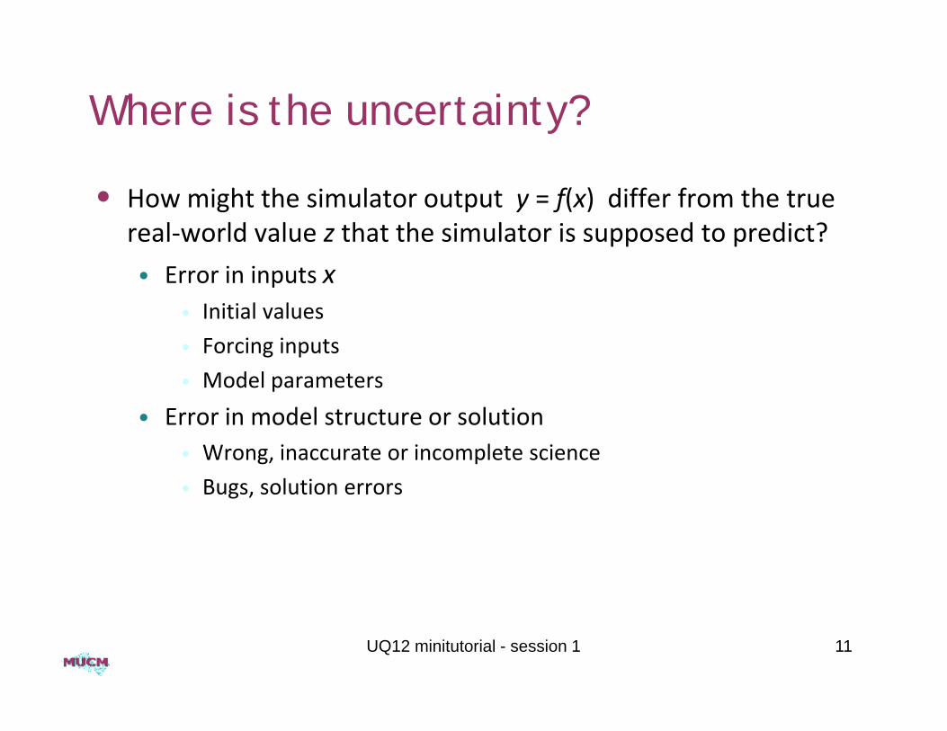
Where is the uncertainty?

• How might the simulator output y = f(x) differ from the true l ld l th t th i l t i d t di t?real‐world value z that the simulator is supposed to predict?

• Error in inputs x• Initial values

• Forcing inputs

• Model parameters

E i d l t t l ti• Error in model structure or solution• Wrong, inaccurate or incomplete science

• Bugs, solution errors


Quantifying uncertainty

• The ideal is to provide a probability distribution p(z) for the t l ld ltrue real‐world value• The centre of the distribution is a best estimate

• Its spread shows how pmuch uncertainty about zis induced by uncertainties on the previous slideon the previous slide

• How do we get this?• Input uncertainty: characterise p(x), propagate through to p(y)

• Structural uncertainty: characterise p(z–y)


More uncertainties

• It is important to recognise two more uncertainties that arise h ki ith i l twhen working with simulators

1 The act of propagating input uncertainty is imprecise1. The act of propagating input uncertainty is imprecise• Approximations are made

• Introducing additional code uncertainty

2. A key task in managing uncertainty is to use observations of the real world to tune or calibrate the modelthe real world to tune or calibrate the model• We need to acknowledge uncertainty due to measurement

error


Code uncertainty – Monte Carlo

• The simplest way to propagate uncertainty is Monte Carlo• Take a large random sample of realisations from p(x)

• Run the simulator at each sampled x to get a sample of outputs

• This is a random sample from p(y)This is a random sample from p(y)

• E.g. sample mean estimates E(Y)

• Even with a very large sample, MC computations are not exact• Sample is an approximation of the population

• Standard error of sample mean is population s d over root n• Standard error of sample mean is population s.d. over root n

• This is code uncertainty

• MC has a built‐in statistical quantification of code uncertainty


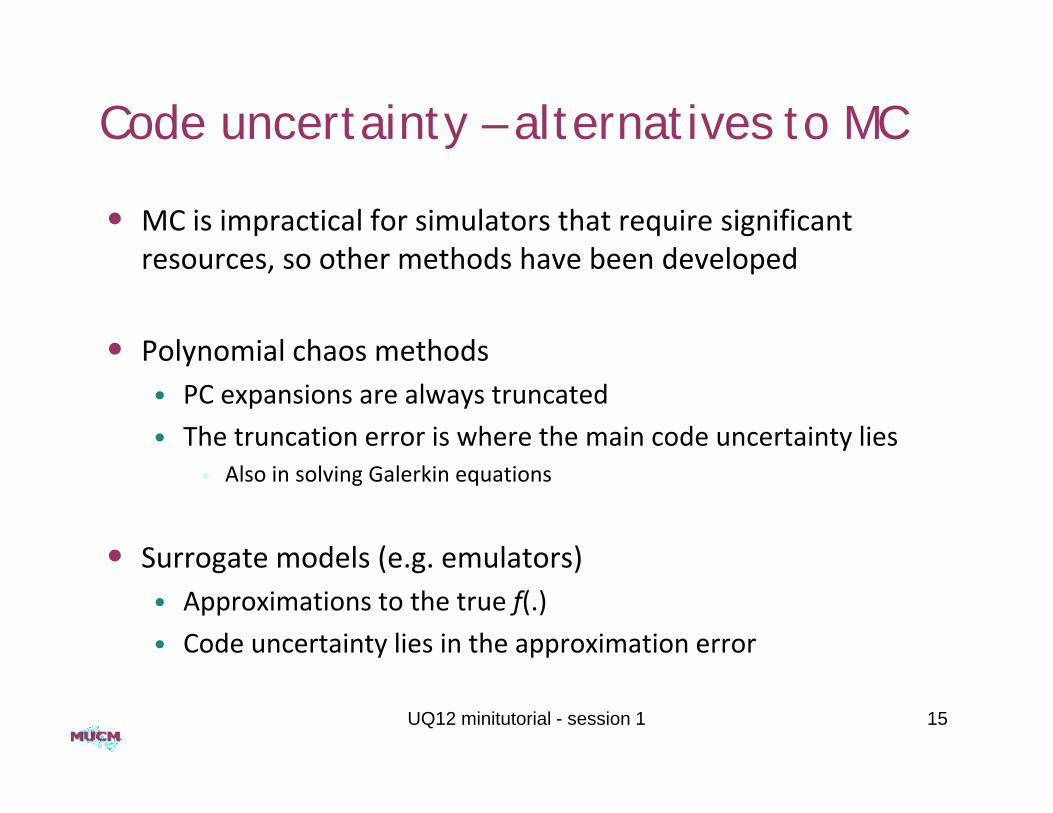
Code uncertainty – alternatives to MC

• MC is impractical for simulators that require significant th th d h b d l dresources, so other methods have been developed

• Polynomial chaos methodsPolynomial chaos methods• PC expansions are always truncated

• The truncation error is where the main code uncertainty lies• Also in solving Galerkin equations

• Surrogate models (e g emulators)• Surrogate models (e.g. emulators)• Approximations to the true f(.)

• Code uncertainty lies in the approximation error


How to quantify uncertainty

• To quantify uncertainty in the true real world value that the i l t i t i t di t d th f ll i tsimulator is trying to predict we need the following steps• Quantify uncertainty in inputs, p(x)

• Propagate to uncertainty in output, p(y)p g y p , p(y)

• Quantify and account for code uncertainty

• Quantify and account for model discrepancy uncertainty

• Engineering/applied maths UQ apparently only deals with the second step• Ironically this is the one step that doesn’t actually involveIronically, this is the one step that doesn t actually involve

quantifying uncertainty!


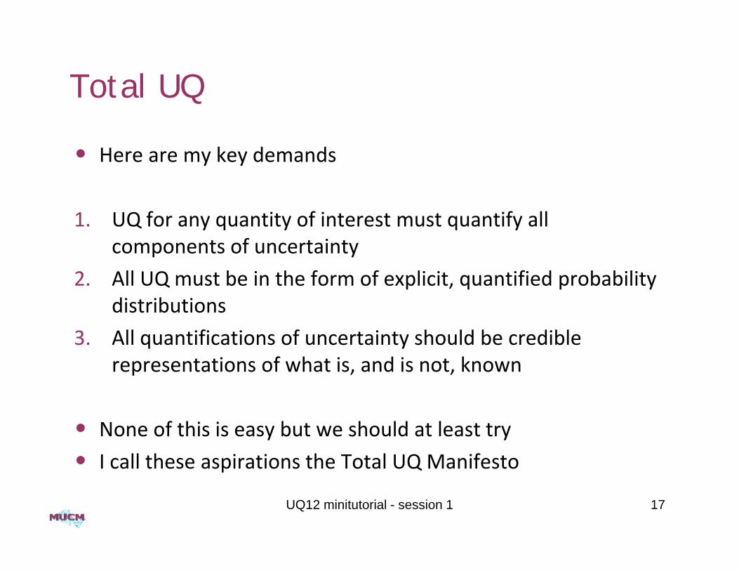
Total UQ

• Here are my key demands

1. UQ for any quantity of interest must quantify all components of uncertaintycomponents of uncertainty

2. All UQ must be in the form of explicit, quantified probability distributions

3. All quantifications of uncertainty should be credible representations of what is, and is not, known

• None of this is easy but we should at least try

• I call these aspirations the Total UQ ManifestoI call these aspirations the Total UQ Manifesto


Managing uncertaintyManaging uncertainty


UQ is not enough

• The presence of uncertainty creates several important tasks /• Engineering/applied maths UQ addresses only one of these

• Managing uncertainty• Uncertainty analysis – how much uncertainty do we have?• Uncertainty analysis how much uncertainty do we have?

• This is the basic UQ task

• Sensitivity analysis – which sources of uncertainty drive overall i d h ?uncertainty, and how?

• Understanding the system, prioritising research

• Calibration – how can we reduce uncertainty?y• Use of observations

– Tuning, data assimilation, history matching, inverse problems

• Experimental design• Experimental design


• Decision‐making under uncertainty – can we cope with uncertainty?uncertainty?• Robust engineering design

• Optimisation under uncertainty


MUCM

• Managing Uncertainty in Complex Models• Large 4‐year UK research grant

• June 2006 to September 2010

• 7 postdoctoral research associates, 4 project PhD students7 postdoctoral research associates, 4 project PhD students

• Objective to develop BACCO methods into a basic technology, usable and widely applicable

• MUCM2: New directions for MUCM• Smaller 2‐year grant to September 2012

• Scoping and developing research proposals• Scoping and developing research proposals


Primary MUCM deliverables

• Methodology and papers moving the technology forward• Papers both in statistics and application area journalsPapers both in statistics and application area journals

• The MUCM toolkit• Documentation of the methods and how to use them• With emphasis on what is found to work reliably across a range of p y g

modelling areas• Web‐based

• Case studies• Three substantial case studies• Showcasing methods and best practice• Linked to toolkit

• E t• Events• Workshops – conceptual and hands‐on• Short courses• Conferences UCM 2010 and UCM 2012 (July 2 4)• Conferences – UCM 2010 and UCM 2012 (July 2‐4)


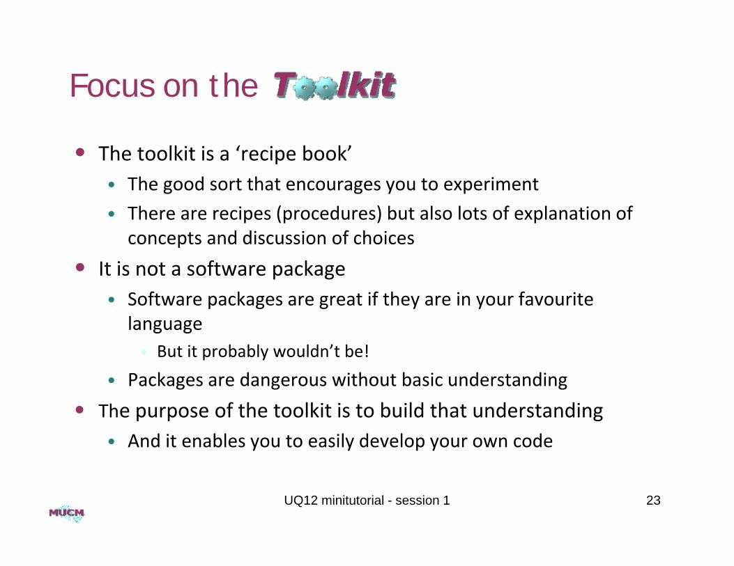
Focus on the

• The toolkit is a ‘recipe book’ • The good sort that encourages you to experiment

• There are recipes (procedures) but also lots of explanation of concepts and discussion of choicesp

• It is not a software package• Software packages are great if they are in your favourite

llanguage• But it probably wouldn’t be!

• Packages are dangerous without basic understanding

• The purpose of the toolkit is to build that understanding• And it enables you to easily develop your own code


Resources

• Introduction to emulators• O'Hagan, A. (2006).

Bayesian analysis of computer code outputs: a tutorial. Reliability Engineering and System Safety 91, 1290‐1300.

• The MUCM website• http://mucm.ac.uk

Th MUCM lki• The MUCM toolkit• http://mucm.ac.uk/toolkit

• The UCM 2012 conferenceThe UCM 2012 conference• http://mucm.ac.uk/UCM2012.html


This minitutorial

• This minitutorial covers the key elements of Total UQ and t i t tuncertainty management

• Emulators• Surrogate models that include quantification of code uncertainty

• Brief outline in this session then details in session 2

• ElicitationTools for rigorous quantification of fundamental uncertainties• Tools for rigorous quantification of fundamental uncertainties

• Introduction to this big field in this session

• Management tools• Sensitivity analysis in session 2

• Calibration and history matching in session 3


A brief case studyA brief case study

Complex emulation and expert elicitation were essential components of this exercise


Example: UK carbon flux in 2000

• Vegetation model predicts carbon exchange from each of 700 pixels over England & Wales in 2000pixels over England & Wales in 2000• Principal output is Net Biosphere Production

• Accounting for uncertainty in inputs• Soil properties• Properties of different types of vegetation• Land usageLand usage

• Also code uncertainty• But not structural uncertainty

• Aggregated to England & Wales total• Allowing for correlations• Estimate 7.46 Mt C (± 0.54 Mt C)( )


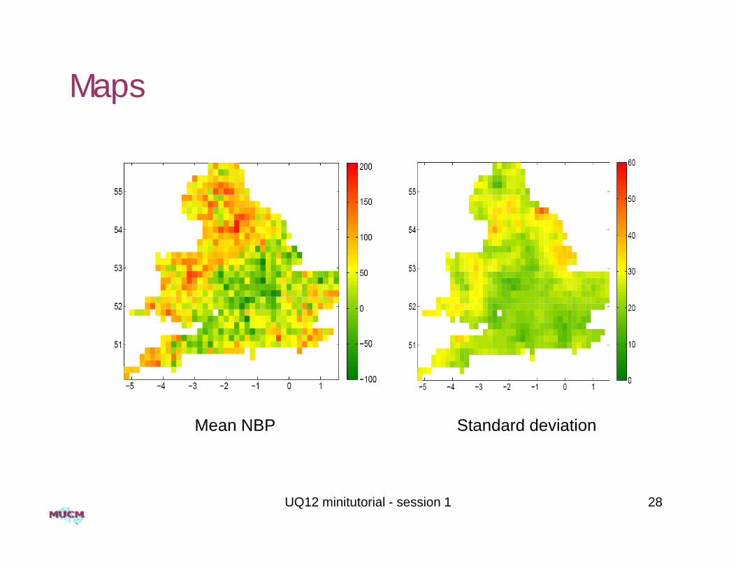
Maps

Mean NBP Standard deviation


England & Wales aggregate

PFTPlug-in estimate

(Mt C)Mean(Mt C)

Variance (Mt C2)

Grass 5.28 4.37 0.2453

Crop 0.85 0.43 0.0327p

Deciduous 2.13 1.80 0.0221

Evergreen 0.80 0.86 0.0048

Covariances -0 0081Covariances -0.0081

Total 9.06 7.46 0.2968


EmulatorsEmulators


So far, so good, but

• In principle, Total UQ is straightforward

• In practice, there are many technical difficulties• Formulating uncertainty on inputs

• Elicitation of expert judgements• Elicitation of expert judgements

• Propagating input uncertainty

• Modelling structural error

• Anything involving observational data!

• The last two are intricatelyThe last two are intricately linked

• And computation


The problem of big models

• Tasks like uncertainty propagation and calibration require us t th i l t tito run the simulator many times

• Uncertainty propagation• Implicitly, we need to run f(x) at all possible xp y, f( ) p

• Monte Carlo works by taking a sample of x from p(x)• Typically needs thousands of simulator runs

• C lib ti• Calibration• Traditionally done by searching x space for good fits to the data

• Both become impractical if the simulator takes more than a pfew seconds to run• 10,000 runs at 1 minute each takes a week of computer time

W d ffi i t t h i• We need a more efficient technique


More efficient methods

• This is what UQ theory is mostly about

• Engineering/Applied Maths UQ• Polynomial chaos expansions of random variables

• Approximate by truncatingApproximate by truncating

• Thereby build an expansion of outputs

• Compute by Monte Carlo etc. using this surrogate irepresentation

• Statistics UQ• Gaussian process emulation of the simulator• Gaussian process emulation of the simulator

• A different kind of surrogate

• Propagate input uncertainty through surrogate

• By Monte Carlo or analyticallyUQ12 minitutorial - session 1 33

Gaussian process representation

• More efficient approach• First work in early 1980s (DACE)

• Represent the code as an unknown function • f( ) becomes a random process• f(.) becomes a random process• We generally represent it as a Gaussian process (GP)

• Or its second‐order moment version

• Training runs• Run simulator for sample of x values• Condition GP on observed data• Condition GP on observed data

• Typically requires many fewer runs than Monte Carlo• And x values don’t need to be chosen randomly


Emulation

• Analysis is completed by prior distributions for, and posterior ti ti f h testimation of, hyperparameters

• The posterior distribution is known as an emulator of the computer simulator• Posterior mean estimates what the simulator would produce for

any untried x (prediction)any untried x (prediction)• With uncertainty about that prediction given by posterior

variance

• Correctly reproduces training data• Gets its UQ right!

• An essential requirement of credible quantificationq q


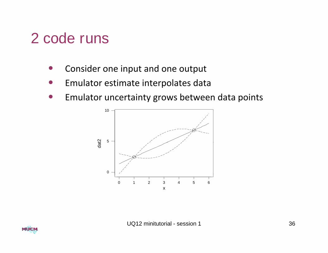
2 code runs

• Consider one input and one output

10

• Emulator estimate interpolates data

• Emulator uncertainty grows between data points10

5t2

0

dat

6543210x


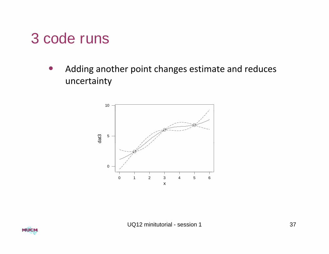
3 code runs

• Adding another point changes estimate and reduces t i t

10

uncertainty

5

dat3

0

6543210x


5 code runs

• And so on

9

88

7

6

5

4dat5

3

2

1

0

6543210x


Then what?

• Given enough training data points we can in principle emulate any simulator output accuratelyany simulator output accurately• So that posterior variance is small “everywhere”• Typically, this can be done with orders of magnitude fewer

d l th t diti l th dmodel runs than traditional methods• At least in relatively low‐dimensional problems

• Use the emulator to make inference about other things of interest• E.g. uncertainty analysis, sensitivity analysis, calibration

• The key feature that distinguishes an emulator from otherThe key feature that distinguishes an emulator from other kinds of surrogate• Code uncertainty is quantified naturally

And credibly• And credibly


Elicitation principlesElicitation principles


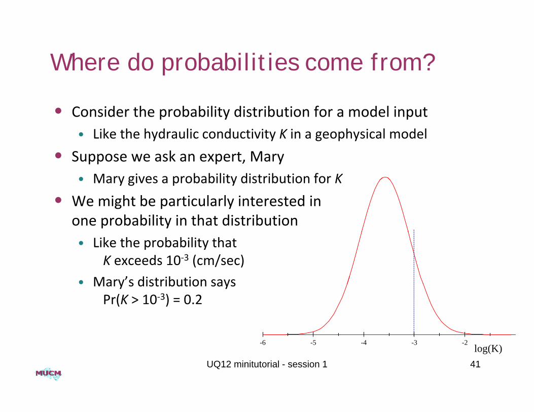
Where do probabilities come from?

• Consider the probability distribution for a model input• Like the hydraulic conductivity K in a geophysical model

• Suppose we ask an expert, Mary • Mary gives a probability distribution for K• Mary gives a probability distribution for K

• We might be particularly interested inone probability in that distribution• Like the probability that

K exceeds 10‐3 (cm/sec)

• Mary’s distribution says• Mary s distribution says Pr(K > 10‐3) = 0.2

-6 -5 -4 -3 -2log(K)


How can K have probabilities?

• Almost everyone learning probability is taught the frequency i t t tiinterpretation• The probability of something is the long run relative frequency

with which it occurs in a very long sequence of repetitions

• How can we have repetitions of K?• It’s a one‐off, and will only ever have one value

’ h i l ’ i d i• It’s that unique value we’re interested in

• Mary’s distribution can’t be a probability distribution in that sensesense

• So what do her probabilities actually mean?• And does she know?


Mary’s probabilities

• Mary’s probability 0.3 that K > 10‐3 is a judgement3• She thinks it’s more likely to be below 10‐3 than above

• So in principle she would bet even money on it

• In fact she would bet $2 to win $1 (because 0.7 > 2/3)

• Her expectation of around 10‐3.5 is a kind of best estimate• Not a long run average over many repetitions

• H b biliti i f h b li f• Her probabilities are an expression of her beliefs

• They are personal judgements• You or I would have different probabilitiesYou or I would have different probabilities

• We want her judgements because she’s the expert!

• We need a new definition of probability


Subjective probability

• The probability of a proposition E is a measure of a person’s d f b li f i th t th f Edegree of belief in the truth of E• If they are certain that E is true then Pr(E) = 1

• If they are certain it is false then Pr(E) = 0y ( )

• Otherwise Pr(E) lies between these two extremes

• Exercise


Subjective includes frequency

• The frequency and subjective definitions of probability are tiblcompatible

• If the results of a very long sequence of repetitions are available, they agree, y g• Frequency probability equates to the long run frequency

• All observers who accept the sequence as comprising titi ill i th t f th i ( lrepetitions will assign that frequency as their (personal or

subjective) probability for the next result in the sequence

• Subjective probability extends frequency probability• But also seamlessly covers propositions that are not repeatable

• It’s also more controversial


It doesn’t include prejudice etc!

• The word “subjective” has derogatory overtones• Subjectivity should not admit prejudice, bias, superstition,

wishful thinking, sloppy thinking, manipulation ...

• Subjective probabilities are judgements but they should be j p j g ycareful, honest, informed judgements• As “objective” as possible without ducking the issue

i b i• Using best practice• Formal elicitation methods

• Bayesian analysis

• Probability judgements go along with all the other judgements that a scientist necessarily makes

A d h ld b d f i th f l h t d• And should be argued for in the same careful, honest and informed way UQ12 minitutorial - session 1 46

But people are poor probability judges

• Our brains evolved to make quick decisionsHeuristics are short cut reasoning techniques• Heuristics are short‐cut reasoning techniques

• Allow us to make good judgements quickly in familiar situations• Judgement of probability is not something that we evolved to

do well• The old heuristics now produce biases

• Anchoring and adjustment• Anchoring and adjustment

• Availability

• Representativeness

• The range‐frequency compromise

• Overconfidence


Anchoring and adjustment

• When asked to make two related judgements, the second is ff t d b th fi taffected by the first• The second is judged relative to the first

• By adjustment away from the first judgementy j y j g

• The first is called the anchor

d ll d• Adjustment is typically inadequate• Second response too close to the first (anchor)

• Anchoring can be strong even when obviouslyAnchoring can be strong even when obviouslynot really relevant to the second question


Availability

• The probability of an event is judged more likely if we can i kl b i t i d i t f itquickly bring to mind instances of it

• Things that are more memorable are deemed more probable• High profile train accidents in the UK lead people to imagine rail travel is more risky than it really is

• My judgement of the risk of dying from a particular disease will be increased if I know (of) people who have the disease or have died from it


Representativeness

• An event is considered more probable if the components of it d i ti fit t thits description fit together• Even when the juxtaposition of many components is

actually improbable

• “Linda is 31, single, outspoken and very bright. She studied philosophy at university and was deeply concerned with issues of discrimination and social justice. Is Linda …of discrimination and social justice. Is Linda …• “A bank teller?

• “A bank teller and active in the feminist movement?”

Th d i f j d d b bl h h fi• The second is often judged more probable than the first

• We are a story‐telling species

• This is also called the conjunction fallacyThis is also called the conjunction fallacy


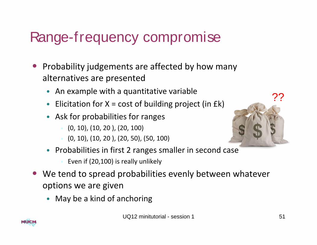
Range-frequency compromise

• Probability judgements are affected by how many lt ti t d

??

alternatives are presented• An example with a quantitative variable

• Elicitation for X = cost of building project (in £k)g p j ( )

• Ask for probabilities for ranges • (0, 10), (10, 20 ), (20, 100)

• (0 10) (10 20 ) (20 50) (50 100)• (0, 10), (10, 20 ), (20, 50), (50, 100)

• Probabilities in first 2 ranges smaller in second case• Even if (20,100) is really unlikely

• We tend to spread probabilities evenly between whatever options we are given• May be a kind of anchoring• May be a kind of anchoring


Overconfidence

• It is generally said that experts are overconfident• When asked to give 95% interval, say, then far fewer than 95%

contain the true value

• Several possible explanationsThe image cannot be displayed. Your computer may not have enough memory to open the image, or the image may have been corrupted. Restart your computer, and then open the file again. If the red x still appears, you may have to delete the image and then insert it again.

p p• Wish to demonstrate expertise

• Anchoring to a central estimate

• Difficulty of judging extreme events

• Not thinking ‘outside the box’• Expertise often consists of specialist heuristicsExpertise often consists of specialist heuristics

• Situations we elicit judgements on are not typical


• Probably over‐stated as a general phenomenon• Experts can be under‐confident if afraid of consequences

• A matter of personality and feeling of security

• Some evidence that people are not over‐confident if asked for p pintervals of moderate probability• E.g. 66% or 50%

• Evidence of over confidence is not from real experts making• Evidence of over‐confidence is not from real experts making judgements on serious questions • Students and ‘almanac’ questions

• Good elicitation practice needs to recognise these problems• Answers depend on how the questions are posed

• Protocol should avoid or minimise biases• Protocol should avoid or minimise biases


Elicitation practiceElicitation practice


Why elicit distributions?

• Occasionally, we want expert opinion about a discrete itiproposition

• The Democrats will win the next US presidential election

• There is, or has at one time been, life on Mars, ,

• Then a single probability needs to be elicited

• Mostly, though, we are interested in opinion babout an uncertain quantity• The mean response of patients to a new drug

• The increase in global temperature caused by a doubling ofThe increase in global temperature caused by a doubling of atmospheric CO2

• Then we need to elicit a probability distribution

• In fact, we are often interested in several quantities55UQ12 minitutorial - session 1

Too many probabilities!

• We’ll stick to a single quantity for now

• One way to think of a distribution for a quantity X is as a set of probabilities• Pr(X < x) for all possible x valuesPr(X < x) for all possible x values

• That’s a lot of probabilities to elicit!

• If we sat down to elicit them one by one, the interrogation would never finish!• And we’d have serious anchoring

problems!problems!

• We need a pragmatic approach


A pragmatic approach

• Animal welfare – what proportion of a herd is diseased?/• X = incidence/1000 of a parasite

• Expert says Pr(X < 10) = 0.4, Pr(X > 30) = 0.20.20.40.4

• Facilitator fits an inverse gamma

0.4

0 10 30

distribution to the two given probabilities

• Check expert agrees Pr(X < 20) ≈ 0.68

• The usual approach has two steps1. Elicit a few probabilities or other ‘summaries’

2 Fit a distribution to those summaries2. Fit a distribution to those summaries


Elicit a few summaries

• We can just elicit a few probabilities• As in the last example

• Other possible ‘summaries’:• Mean median mode• Mean, median mode

• Often expert is just asked for an ‘estimate’

B t th t b th ti f• But that begs the question of what kind of estimate

• The mean and mode are not recommended 6recommended

• Asking for the median is OK (value with probability 0.5 on either side)

Mode = 6 Median = 13Mean = 30

either side)


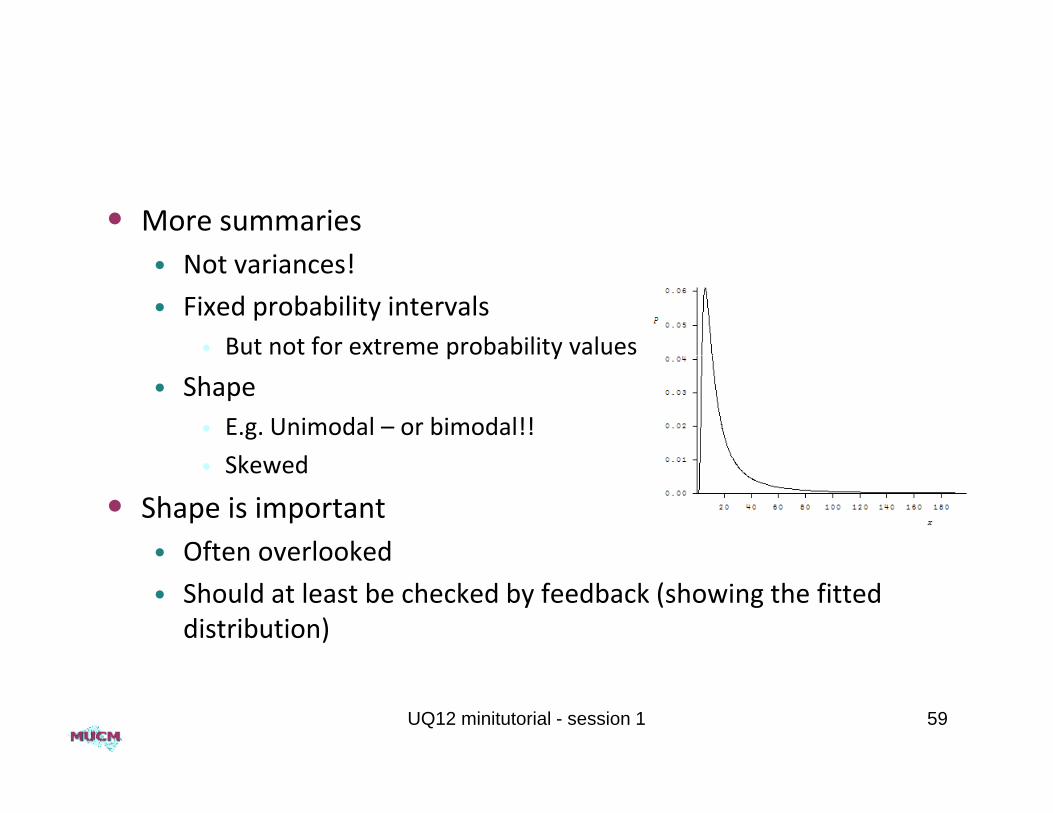
• More summaries• Not variances!

• Fixed probability intervals • But not for extreme probability valuesp y

• Shape• E.g. Unimodal – or bimodal!!

Sk d• Skewed

• Shape is important• Often overlookedOften overlooked

• Should at least be checked by feedback (showing the fitted distribution)


Then fit a distribution

• Any convenient distribution• As long as it fits the elicited summaries adequately

• At this point, the choice should not matter• The idea is that we have elicited enough• The idea is that we have elicited enough

• Any reasonable choice of distribution will be similar to any other

• Elicitation can never be exact• The elicited summaries are only approximate anyway

• If the choice doesmatterd ff f d d b d ff h• i.e. different fitted distributions give different answers to the

problem for which we are doing the elicitation

• then we need to elicit more summaries


The SHELF system

• SHELF is a package of documents and simple software to aid li it tielicitation• General advice on conducting the elicitation

• Templates for recording the elicitationp g• Suitable for several different basic methods

• Annotated versions of the templates with detailed guidance

S R f i f fi i di ib i d idi f db k• Some R functions for fitting distributions and providing feedback

• SHELF is freely available and we welcome comments and suggestions for additionsgg• Developed by Jeremy Oakley and myself

• R functions by Jeremy

// /UQ12 minitutorial - session 1 61

• http://tonyohagan.co.uk/shelf

Contents

• SHELF Overview_v2.0

• SHELF Pre elicitation Briefing• SHELF Pre‐elicitation Briefing

• SHELF Pre‐elicitation Form + version with notes

• SHELF 1 (Context) + version with notes

• SHELF 2 (Distribution) Q + version with notes

• SHELF 2 (Distribution) QP + version with notes

• SHELF 2 (Distribution) R + version with notes( )

• SHELF 2 (Distribution) RP + version with notes

• SHELF 2 (Distribution) T + version with notes

• SHELF 2 (Distribution) TP + version with notes• SHELF 2 (Distribution) TP + version with notes

• SHELF2 Distribution fitting instructions

• shelf2.R


Example

• We will now look at a hypothetical example of using SHELF• Using a simplified form for a single expert


Where to next

• Two more sessions to come in this minitutorial

• Tomorrow:• Peter Challenor will present Session 2 on building and using

emulators

• Wednesday• I will begin Session 3 on using observations of the real world

l b d h kprocess – calibration and other tasks

• Ian Vernon will finish with a case study on a grand scale –history matching a galaxy formation model to observations of the universe


Another conference

• UCM 2012

• Still open for poster• Still open for posterabstracts

• Early bird registrationdeadline 30th April

• http://mucm.ac.uk/ucm2012


emulation, elicitation and calibration · 2012-04-16 · what is uq? • uncertainty quantification...

Documents