enclosure 10 c.d.i. technical note no. 05-45

Enclosure 10

C.D.I. Technical Note No. 05-45, "Extrapolation of QC1and QC2 Steam Dryers Loads to 2957 MWt," Revision

0

C.D.I. Technical Note No. 05-45

Extrapolation of QC 1 and QC2 Steam Dryer Loads to 2957 MWt

Revision 0

Prepared by

Continuum Dynamics, Inc.34 Lexington Avenue

Ewing, NJ 08618

Prepared under Purchase Order No. 403726 for

Exelon Generation LLC4300 Winfield Road

Warrenville, IL 60555

Approved by

Alan J. Bilanin

December 2005

Extrapolation Procedure

Exelon asked Continuum Dynamics, Inc. (C.D.I.) to extrapolate their acoustic circuit modelpredicted steam dryer loads for Quad Cities Unit 1 (QC1) and Unit 2 (QC2) to a maximumpower level of 2957 MWt. These results could then be compared to extrapolation factorsgenerated for Exelon using pressure sensor data (in QC2) and main steam line strain gage data(in QC] and QC2), as reported in [1]. This technical note summarizes the extrapolationprocedure used here and presents its results.

C.D.I. sought to provide independent confirmation of the results reported in [1], by restricting thefrequency range of interest between 145 Hz and 165 Hz, power levels between OLTP and EPU,and pressure nodes above the skirt.

The methodology utilized by C.D.I. to determine separate extrapolation factors for QC 1 and QC2accessed the strain gage data recorded from the QCl and QC2 main steam lines during powerascent, following the installation of replacement steam dryers. Data from three power levelswere selected from each unit. The test conditions chosen are shown in Table 1.

Table 1. Power levels examined for extrapolation to 2957 MWt.

Quad Cities Unit Test Condition Power LevelNumber Number (MWt)

1 TC11 26411 TC12 27651 TC15_A 28872 TC37 27542 TC39 28312 TC41 2887

The data from each test condition were used to develop low resolution loads on the replacementsteam dryer, the outer bank hood in front of the main steam lines, and the cover plate below themain steam lines. The Modified 930 MWe Acoustic Circuit Model was used in the analysis, andthe loads included only the frequency contributions from 145 Hz to 165 Hz. Nodes on eachdryer were used to develop linear curve fits separately, as a function of power level at each node.The data were then extrapolated to maximum power to estimate the pressure load to be expectedand the percentage increase in load from the highest power level measured.

The replacement steam dryer was represented by low resolution nodes on the dryer surfaces asillustrated in Figures 1 to 4. The nodes averaged in front of each main steam line were:

MSL A: Nodes 119, 120, 121, 124, 125, 126, 133, 134, 135, 144, 141MSL B: Nodes 117, 118, 119, 122, 123, 124, 131, 132, 133, 140, 144MSL C: Nodes 9, 4, 15, 16, 17, 20, 21, 22, 25, 26, 27MSL D: Nodes 4, 10, 17, 18, 19, 22, 23, 24, 27, 28, 29

2

The extrapolation process at each node involved the following steps:

1. For each dryer the acoustic circuit model low resolution loads were used to predict thepressure load anticipated at each power level.

2. The three pressures were used in a linear least squares curve fit. The three power levels foreach dryer were selected in anticipation of an approximately uniform power increase betweenpower levels. The curve fit then generated the constants A and B in the equation

P=A+BW

where P is pressure and W is power level. Correlation coefficients for this operation variedbetween averages of 0.69 and 0.97 on the dryer nodes opposite the four main steam lines.

3. The linear curve fit was then extrapolated to WM = 2957 MWt by the equation

PM = A + BWM

to obtain the pressure PM predicted at 2957 MWt.

4. A percentage increase was formed involving PM and the interpolated pressure P3 at W3 = 2887MWt (P3 = A + BW3), such that

Percentage Increase [ 100{PM P3 ]

The nodal results found by averaging these predictions in front of the four main steam lines aresummarized in Table 2.

Table 2. Average percentage increase in power level to 2957 MWt.

Main Steam Extrapolation ExtrapolationLine Percentage for QC1 Percentage for QC2

A 8.9 23.8B 8.8 24.3C 9.2 3.8D 10.5 3.6

Summary

A linear least squares curve fit to low resolution predictions on the replacement dryer at QC 1 andQC2 resulted in a tabulation of the range of extrapolation percentages for each unit. Maximumvalues were 10.5 percent for QCI and 24.3 percent for QC2. Comparison with the resultsgenerated from [1] will provide the confirmation needed by Exelon.

3

As further confirmation of these findings, C.D.I. examined the percentage increase in thepressure signal measured in a scaled facility simulating a single main steam line at QC2 [2]. Forthis comparison the test facility was run at Mach numbers approximating the main steam lineflow velocity at 2887 MWt and 2957 MWt, for the Dresser valves, and a simple percentageincrease was calculated. On average, the peak pressure on the Dresser valves increasedapproximately 25 percent, from 2887 MWt to 2957 MWt. These findings are consistent with thelinear least squares curve fit model applied to the low resolutions loads on QC2.

References

1. LMS. 2005. Quad Cities New Design Steam Dryer Methodology for Stress Scaling FactorsBased on Extrapolation from 2885 MWt to 2957 MWt of Unit #2 / Dryer #1 Data. ReportNo. GENE-0000-0046-8129-02-P (Revision 1).

2. Continuum Dynamics, Inc. 2005. Mitigation of Pressure Oscillations in the Quad CitiesSteam Delivery System: A Subscale Single Main Steam Line Investigation of StandpipeBehavior. C.D.I. Report No. 05-29.

4

6 6 ~76 8~2 9:~ 98-

108 .116

19

10

4 17

9

3 2

1 8

135

134

I _31L L 431_ _ _5?[ _ 65 _75 981 _ 9?7 _1071 1151 133

† 141

4I 0

..1...4016

30

132

131

42

10658 64 74 80 90 96

Figure 1. Bottom plates pressure node locations. The main steam lines are located in the upperright hand corner (MSL A, above node 141), the lower right hand corner (MSL B,above node 140), the lower left hand corner (MSL C, above node 9), and the upperleft hand corner (MSL D, above node 10).

5

Cof

6;3 63-~~ 85I[- -101

1i1

121No

I

I

III

II

II

II

II

- - - T- - -

II

II

II

II

I

1 121-f ' hi i $ tt0:1 120

62 - -- 1.. - _ S 1- 0 I _. 11;. 119

.____I_

,','

11 I,

I 1 -0 . b y t_

II

I

1 17 I'

9 9, j 109

61 67 7 , 3

Figure 2. Top plates pressure node locations. The main steam lines are located in the upperright hand corner (MSL A, below node 120), the lower right hand corner (MSL B,below node 118), the lower left hand corner (MSL C, below node 26), and the upperleft hand corner (MSL D, below node 28).

6

Coy-

121 S

r 3126 .

Fiur 3XSane plte rersningtedyrbnsI

7

141

Figure 4. Skirt plates.

8

Enclosure 11

SIA Report SIR-05-223, "Comparison of Quad CitiesUnit 1 and Quad Cities Unit 2 Main Steam Line Strain

Gage Data," Revision I

Structural Integrity Assodates, Inc.

6855 S. Havana StreetSuite 350Centennial, CO 80112-3868Phone: 303-792-0077Fax: [email protected]

July 18, 2005SIR-05-223 Revision IKKF-05-037

Mr. Robert StachniakExelon Nuclear4300 Winfield RoadWarrenville, IL 60555

Subject: Comparison of Quad Cities Unit 1 and Quad Cities Unit 2 Main Steam Line StrainGage Data

Dear Rob:

This letter report contains a comparison of the Quad Cities Unit 1 (QC1) and Quad Cities Unit 2(QC2) strain gage data obtained during the power ascensions that occurred during Spring 2005.

Background

Main steam line strain gage data was obtained during the June 2005 power ascension at QC1 [1].This data was used as input to the acoustic line analysis that determines the forcing function onthe steam dryer. Prior to the power ascension, strain gages were installed on each of the fourmain steam lines (MSLs) at two axial locations. At each axial location two strain gage pairs areformed with two gages 1800 apart. The two gages are connected to a Wheatstone bridge in the l/2bridge configuration where the two strain gages will sum to provide higher sensitivity andprovide cancellation of the Poisson effect due to pipe bending. Strain gage were also installed onthe main steam lines at QC2 using the same 1/2 bridge configuration and locations as QC 1.Figures I a and lb shows sketches of the strain gage locations for QCI and QC2 MSL A, B, C,and D.

Objective

The objective of this letter report is to compare the strain gage measurements between the twounits and determine the degree of similarity between the units structural response and pressureexcitation. The data has been analyzed for frequency content (rms spectra), time historycharacteristics (rms, maximum, and minimum), and relationship between orthogonal planes(Cross Spectral Density). Figures la and lb provide sketches of the four MSL for both unitswith the strain gage locations designated.

Austin, TX Charlotte, NC512-533-9191 704-597-5554

N. Stonington, CT San Jose, CA Silver Spring, MD Sunrise, FL860-599-6050 408-978-8200 301-445-8200 954-572-2902

Uniontown, OH Whittier, CA330-899-9753 562-944-8210

Mr. Robert Stachniak July 18, 2005SIR-05-223 Rev. I/KKF-05-037 Page 2 of 33

Combined Spectra for QC1 and QC2

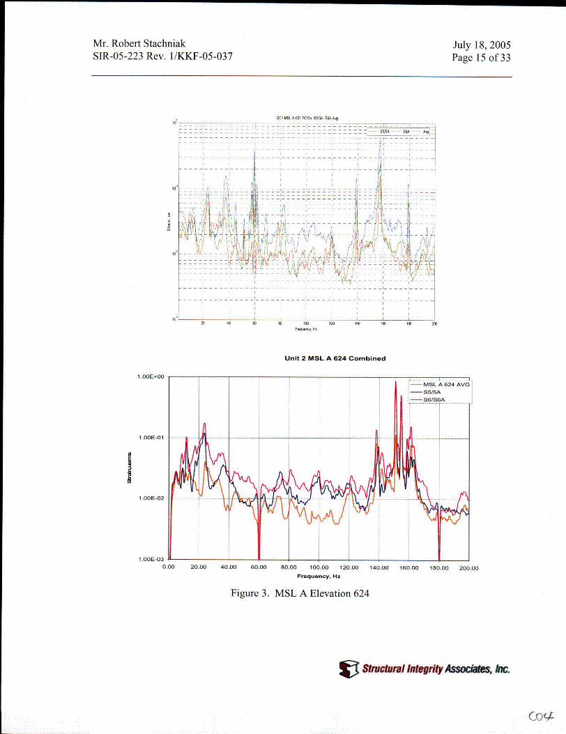
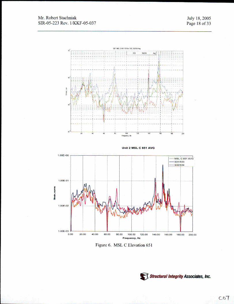
Figures 2 through 9 provide the combined spectra (individual 1/2 or 1/4 bridge with their average)for the 651' and 624' elevations on each MSL. The figures provide the QC1 and QC2 spectra forthe unique location for purposes of visual observations. A review of the spectra at each locationprovides the following observations. In addition, Table 1 summarizes the observations.

1. The profiles of the spectra are similar in that the overall amplitudes across the spectrumare the same except for QC 1 A, C and D 651 where each has relatively higher amplitudesat 78.6 and 157.7 Hz. For example, the frequency spectra for D624 (Figure 9) has a verysimilar shape and amplitudes for both QCI and QC2; both units at this location havelarge amplitudes.

2. QCl has typically a very broad unique peak at 157.7 Hz whereas QC2 has 3 to 5narrower peaks in the range of 150 to 160 Hz (see Figure 2 for a comparison of QCI toQC2).

3. The predominant frequencies occurred in most of the spectra for QCI at 23, 78.6, 138.7and 157.7 Hz and for QC2 at 23, 139.2, 150.9 and 154.8 Hz.

4. A review of Table 1 shows that QCI has the highest amplitudes in the low frequencyrange (15 to 35 Hz) and in the higher frequency range (135 to 160 Hz) the highamplitudes are evenly split between QC1 and QC2. The most number of peaks in the 135to 160 Hz range is always QC2.

RMS Values for QC1 and QC2

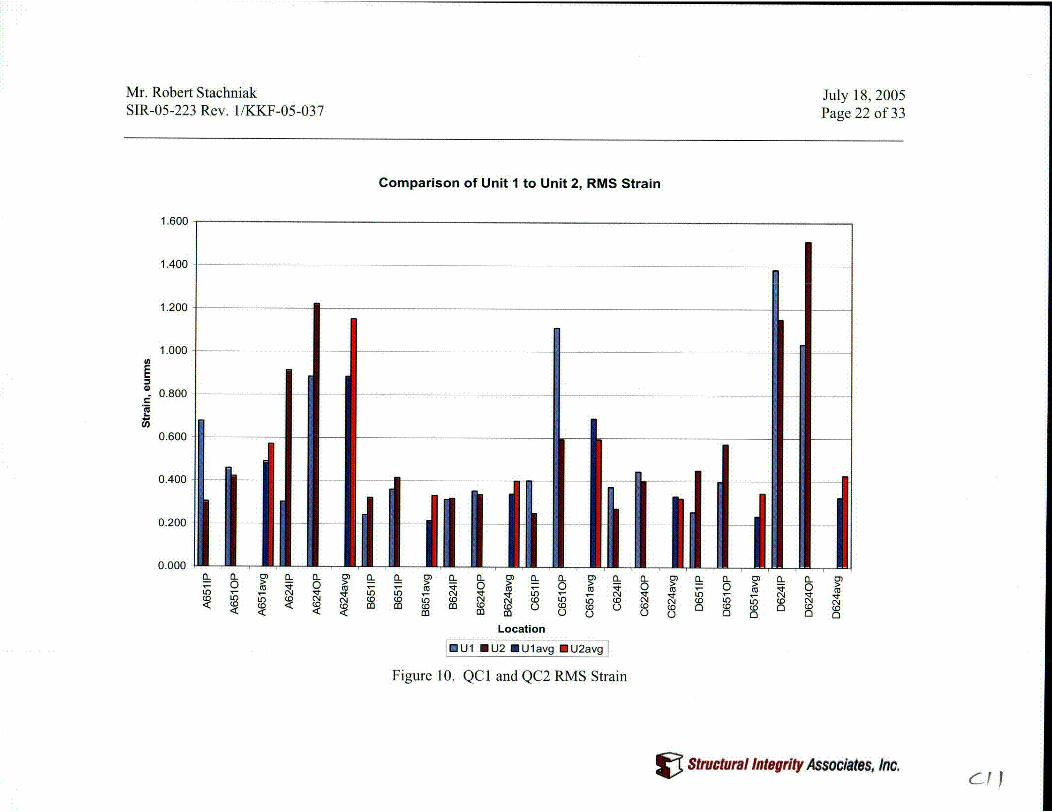
Table 2 provides the RMS, Max-Min and Average amplitudes for the time histories of individualstrain gage bridges and the average of the orthogonal bridges for each unit. The RMS is the root-mean-square value of the filtered strain time history over a bandwidth of 2 to 200 Hz in units ofjis,. The Max-Min value is the Maximum positive value minus the Maximum negative valueover a bandwidth of 2 to 200 Hz for the entire time history. The Max-Min value isconservatively referred to in this document, as peak-to-peak, whereas the term peak-to-peaktypically refers to consecutive peaks and valleys in the time history. The Average value is theaverage of the In-plane (IP) and the Out-of-plane (OP) time histories. The RMS, max-min, andaverage are characteristics of the time history, not the frequency spectra.

Table 2 is graphically portrayed in Figure 10 as a bar chart. General observations of Table 2(Figure 10):

1. Many of the locations have similar RMS responses except for QCI-A651IP, C651IP,C65 lOP and D6241P and QC2-A6241P, A6240P, and D6240P where there are largerdifferences. When averaged, the RMS values are much closer except for a largeamplitude difference for A624avg.

V Strduocral ntegrt AssOates, hc.

Mr. Robert Stachniak July 18, 2005SIR-05-223 Rev. l/KKF-05-037 Page 3 of 33

2. In Table 2, the averages of all the RMS/Max-Min values, and the IP and OP values,separately, are provided for both QC 1 and QC2 along with the averages of the averageRMS and Max-Min (M-M). Other than the average of the average RMS and Max-Min,QCl and QC2 are extremely close in all the statistical values. For the averaged RMSavg,QC2 is 18% greater than QC1.

3. For both the RMSavg and Max-Minavg (M-Mavg) the OP is 30 to 40% greater for bothunits.

4. Figure 11 is a graph of the ratios of the RMS averages (Table 2) for the 651 to 624elevations for each unit. The results show that the ratios are similar for each unit. Thisfigure shows that the 624 response is higher than the 651 response, except for MSL C.For MSL C, the 651 response is almost twice as large as the 624 response for both units.

Half Bridge Phase Relationships

The cross spectral density (CSD) between the two orthogonal bridges for all locations wascalculated for both units. If only a quarter bridge was available at a location, it was used in lieuof the half bridge. The cross spectral density is calculated from the power spectral density (PSD)for each orthogonal bridge; the two complex functions are multiplied and graphed as magnitudeand phase versus frequency, where the magnitude is proportional to the strain squared.

The magnitude accentuates frequencies that are common to both bridges. The phase provides therelationship in time between the two bridges at each frequency; i.e., one bridge leads or lags theother by the phase. Figures 12 and 13 are typical CSD plots for QCl and QC2, respectively.For each figure the top plot is the relative magnitude and the bottom is phase.

From similar figures for each elevation, the CSD magnitude and phase at predominatefrequencies were tabulated in Table 3. A quick overview of the table indicates that the phasevaries significantly for the same frequency at different locations. Figure 14 provides acomparison of the phase for 157.7 Hz (QC1) and 154.8 Hz (QC2) for each location. The plotshows the absolute phase since the polarity only indicates which bridge is leading or lagging, butin averaging the two bridges the effect is the same.

It is observed that at each location except A651 the phase is relatively close in amplitude in the10 to 400 range. For example the effect on amplitude of averaging two sine waves with the sameamplitude 45 degrees out of phase is approximately an 8% decrease in amplitude, for a 90 degreephase difference it is -30%. The effect is proportional to the cosine of the phase-angle/2.

Figure 15 provides a graph of the CSD magnitude for the same frequencies discussed above.Note the CSD magnitude is plotted on a log scale. Except for A624 the QC1 magnitude isalways greater and sometimes significantly greater for the 157.7 Hz than the QC2 154.8 Hz

!C Sfmcbural IntegrfrAssoc=tesw ka


response. The higher CSD magnitude indicates a stronger response over the entire time historybetween the two orthogonal amplitudes at the 157.7 Hz response.

The other frequencies in Table 3 did not provide enough information for comparison of the unitsor did not have a counterpart in each unit.

QC2 Quarter Bridge Strain Gage Data

The QC2 strain gages did not experience the same number of failures that occurred at QC 1, thus,1/4 bridge data was recently obtained at QC2. On July 6, 2005, Exelon recorded the l/2 bridge datafor main steam lines B and C, and then reconfigured the half bridges on the same main steamlines into quarter bridges and recorded ¼ bridge data on July 7, 2005 [4]. An initial review ofthis data shows that all the strain gages are functioning.

For QC2 MSL C 651, the 1/4 bridge data was combined for the IP (S31/33) and OP (S32/34) tocreate '/2 bridge results. Figures 16 and 17 show the equivalent l/2 bridge results based on the 1/4

bridge data. A fair comparison of the combined 1/4 bridge results to the actual '/2 bridge data wasnot possible as there were no two datasets gathered sufficiently close in time and power level.

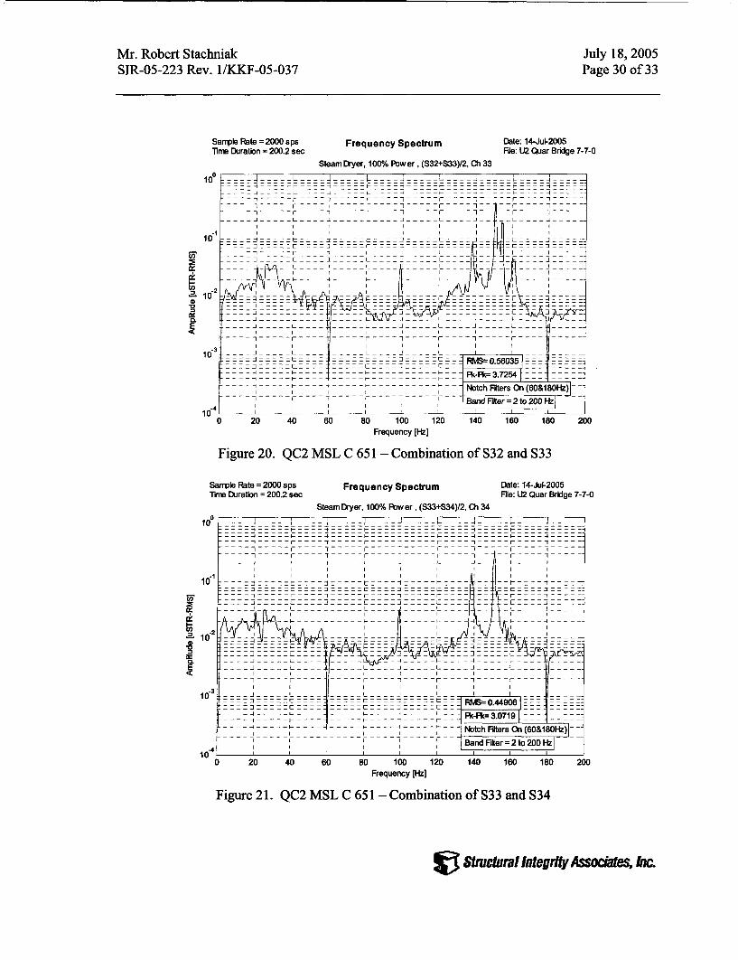
The effect of losing strain gages in QC1 and using 1/4 bridges with the '/2 bridge to produceaverages appears by the close results between the units to be insignificant; this is confirmed byusing the QC2 ¼ bridge data. A review of the QC2 1/4 bridge data confirms that the combinationof a 1/4 bridge and a /2 bridge (Figure 18) produces results that are almost identical to theaveraged two equivalent /2 bridge results (Figure 19). Other combinations of 1 bridge straingages was also performed for QC2 MSL C 651 to investigate the effect of losing more than onestrain gage at a location. Since QC1 MSL C 651 S31 had failed, the remaining combinations oftwo 1/4 bridges that include IP and OP are S32/33 and S33/34. Thus, the QC2 MSL C 651combination of S32/33 and S33/34 was generated and is shown in Figures 20 and 21,respectively. A review of the S32/33 combination shows that the results are similar to theequivalent two l/2 bridge combination (Figure 18), whereas the S33/34 combination shows someevidence of missing frequency content (e.g., 154.8 Hz and 161 Hz).

The four functioning gages per elevation on QC2 MSL C allowed the computation of amplitudesbased PSDs and phase angles based CSDs using S31 as a reference. The two frequencies (150.9Hz and 154.8 Hz) were selected based on statements made earlier in this report (Page 2) and theresulting amplitude and phase values are listed in the table below.

S3 Structural in1egrt Associes, Am

Mr. Robert StachniakSIR-05-223 Rev. I/KKF-05-037

July 18, 2005Page 5 of 33

150.9 Hz 154.8 HzLocation Amplitude Phase Amplitude Phase

uSTR2/Hz deg uSTR2/Hz deg

(referen 0.104 0 0.017 0S32 0.115 67 0.032 19S33 0.233 69 0.059 -7S34 0.105 84 0.033 177S35 0.004 -154 0.025 44S36 0.044 -42 0.008 127

S35A 0.051 144 0.008 -135S36A 0.028 -48 0.015 5

The resulting pipe cross-sectional movement is graphically represented on Figures 23 and 24.The point number assignments used in these plots and their relation to the strain gages are shownon Figure 22. The upper elevation (651) shows more movement at these frequencies than thelower (621) elevation. This may be in part due to the fact that this location is closer to the vesseland may be exposed to more dynamic fluid behavior internally. At 150.9 Hz, El 651 appears tobe in a breathing mode while El 621 is showing a small amount of ovaling. At 154.8 Hz, El 651appears to be an ovaling mode while El 621 appears to be closer to a breathing mode at muchlower amplitudes.

Discussion

The MSL piping for both units are for all intents and purposes identical except for some valvelocations and the HPCI connection. The MSL pipe characteristics (pipe size, material,configuration in the plant and in relationship to the vessel) are the same, therefore the dynamicresponse will be similar. In other words the piping's dynamic response (transfer function) isidentical. That is for similar excitation (internal dynamic pressure) the pipes will respond thesame and provide the same vibration and acoustic measurements.

The strain measurements were designed to measure only hoop strain which can consist of zeromode, concentric expansion and contraction and breathing modes such as ovaling and clover leafmodes. The bending mode Poisson effect is canceled by the bridge configuration for two gages,but it appears from the data that it is not significant if a 1/4 bridge is used, since all the majorfrequencies can be accounted for in both the l/2 and 1/4 bridges.

The zero mode and ovaling mode natural frequencies were calculated to be greater than 300 Hz,therefore responses below 300 Hz would be considered a 'forced vibration', a non-resonantvibration. The response of a structure to a forced vibration that is below the first mode ofvibration would be in a mode shape similar to the first mode, assuming the first mode is the leaststiff mode (path of least resistance).

to Stmrtural Integrity Assocaes, kzc


For hoop strain, the least stiff mode would be the ovaling mode. Assuming a uniform load ateach axial location the pipe's hoop strain would follow the pattern of an oval. In orthogonalplanes the pipes should be 180 degrees out of phase. For non-uniform loading bothcircumferentially and axially, the shape may not be a pure oval and may change along the lengthof the pipe depending on the loading distribution.

The results of the CSD analysis did not show a uniform response at the frequencies of interest bythe variation of the phase relationships, but did show similar responses at the same pipe/elevationcombination. This would indicate that the loading of the pipes are similar for both units yet arenon-uniform both axially and circumferentially.

The structural and loading similarities are also shown in the results from the statistical averagingof the RMS and max-min values for the individual bridges. The most telling result that showsthis similarity is the RMS averages provided below in Table 2. In comparing QC1 to QC2 thedifference in the values for each category are less than 8%. Since several of the QC 1 resultsinclude the 1/4 bridges, this implies that the effect of 1/4 versus 1/2 bridge may be minimal. A moredetailed study of the 1/4 bridges available for QCI and QC2 would provide additional insight intothe results of using 1/4 versus 1/2 bridge strains.

Also, included in the table are the relationship between the OP and IP bridges with OP showing a30 to 40% increase in overall response than the IP and again consistent in both plants.

Unit I Unit 2RMS Max-Min RMS Max-Min

Total rms 8.993 72.515 9.456 68.968RMS Avg 0.562 4.532 0.591 4.310RMS HP avg 0.493 3.748 0.498 3.617RMS OP avg 0.631 5.316 0.684 5.004

The Max-Min values are not considered a statistical representative of a time history, since theyare a single, maximum point picked from the positive and negative sides of the time history, yet,even these are consistent. The implication of both units having the RMS and max-min similarityis that the excitation forces for both units are similar with similar loading.

The primary difference in the strain data observed between the units is the actual frequencycontent of the signals. The area where this is most obvious is in the 150 to 160 Hz range whereQCl is observed to have a single strong response at 157.7 Hz and QC2 has several frequencies inthis frequency range, particularly 150.9 and 154.8 Hz. The 154.8 Hz seems to have many of thesame characteristics as the 157.7 Hz, particularly, the phase relationships for the pipe/elevationcombination, but from the CSD magnitude it appears that the QC1 157.7 Hz response is muchstronger than the corresponding 154.8 Hz of QC2.

Stusfctural Integrt Assoce Ina

Mr. Robert Stachniak July 18, 2005SIR-05-223 Rev. 1/KKF-05-037 Page 7 of 33

Another difference between QC1 and QC2 is the strain response at 78.6 Hz observed in threelocations in QC1 at elevation 651 for MSL A, C, and D. The pressure at this frequency maycontribute to the vibration response of the steam dryer.

Conclusion

In conclusion, the strain measurements acquired at both QC1 and QC2 appear to be consistentlysimilar implying a similarity in both the pressure excitation of the piping and the response to theloading. The consistency provides a measure of the quality of the data for both units. The strainresponse at Elevation 624 is larger than that of Elevation 651 for both units except for MSL C.This phenomenon is seen at both units. The consistencies between the main steam line straindata shows that even though there are some structural differences between the two units, bothunits appear to respond the same due to the pressure excitation of the piping.

The effect of losing strain gages in QC1 and using 1/4 bridges with the 12 bridge to produceaverages appears by the close results between the units to be insignificant. A review of the QC2/4 bridge data confirms that the combination of a 1/4 bridge and a /2 bridge produces results thatare almost identical to the averaged two equivalent 1/2 bridge results.

A further understanding of the structural response of the pipe and the pressure distribution in thepipe has been performed which shows that some local shell phenomena are occurring at eachstrain gage location.

If you have any questions, please do not hesitate to contact me at (303) 792-0077.

Prepared By: Reviewed By:

Lawrence S. Dorfman Karen K. Fujikawa, P.E.Associate Associate

Approved By:

Karen K. Fujikawa, P.E.Associate

kkfREFERENCES:

1. Exelon Document No. TIC-1252, Revision 0, "Quad Cities Unit 1 Power Ascension TestProcedure for the Reactor Vessel Steam Dryer Replacement," SI File No. EXLN-20Q-201.

! Structural nlnegrltAssoM , hINC

Mr. Robert Stachniak July 18,2005SIR-05-223 Rev. I/KKF-05-037 Page 8 of 33

2. Exelon TODI No. ODC-05-0225, "Main Steam Line Strain Gauge Failures During QuadCities Unit 1 Startup Testing," SI File No. EXLN-20Q-201.

3. Structural Integrity Associates, Inc. Report SIR-05-208 Revision 2, "Quad Cities Unit 1 MainSteam Line Strain Gage Reductions," SI File No. EXLN-20Q-401.

4. E-mail, from Brian Strub (Exelon) to Karen Fujikawa (SI), dated 7/7/05, "Ibackup has QC2Half Bridge and Quarter Data," SI File No. EXLN-20Q-204.

cc: EXLN-20Q-402Chuck Alguire (Exelon)Guy DeBoo (Exelon)Roman Gesior (Exelon)Keith Moser (Exelon)Kevin Ramsden (Exelon)Brian Strub (Exelon)K. Rach (SI)G. Szasz (SI)

Table 1. Observations of Combined SpectraMost

Max Avg Amplitude Peaks135 -165

Location Profile 15 - 35 hz 135-160 Hz HzA651 similar* U1 U1 U2A624 similar U2 U2 U2B651 similar = U2 U2B624 similar U1 U1 U2C651 similar* U1 U1 U2C624 similar U1 U1 U2D651 similar* U2 U2 U2D624 similar = U2 U2

* Similar other than QCI-78.6 and 157.7 Hz amplitude

StJuVtural teg9rftYAssoWeie ha

Mr. Robert StachniakSIR-05-223 Rev. 1/KKF-05-037

July 18, 2005Page 9 of 33

I3I

SAI

MSLi

Figure 1a. Location of Strain Gages on QC 1 and QC2 MSLs A and B

V3 SMructorallntegrlrAssomaes, ha


July 18, 2005Page 10 of 33

'EI

IE

MSL \J-

Figure lb. Location of Strain Gages on QC1 and QC2 MSLs C and D

C Stuictural IntegrityAssoC&e k


July 18,2005Page 11 of 33

Table 2. QC1 and QC2 RMS and Max-Min ValuesUnit 2Unit 1

DescriptionS1 A651S2/S4 A651S5/S5A A624S6A A624S7/S9 B651S8/SIO B651

SII B624S12/S12AB624

S33 C651

S32/S34 C651S35/S35AC624

S36A C624

S37/S39 D651

S38/S40 D651S41/S41AD624S42/S42AD624

Total rmsRMS AvgRMS IP avgRMS OP avg

Max-RMS Min RMSavg M-Mavg0.678 4.483 --

0.459 4.275 0.490 3.6600.303 2.530 -

0.885 8.120 0.876 5.7300.242 2.177 -- --

0.361 3.004 0.216 1.849

0.314 2.911 ----

0.353 3.138 0.340 5.450

0.401 3.269

1.110 9.629 0.690 5.800

0.371 3.011 ----

0.444 3.774 0.330 1.270

0.256 2.381 ---- ----

0.397 3.524 0.237 2.166

1.382 9.221 ------ ----

1.036 7.066 0.325 2.529Avg 0.438 3.557

8.993 72.5150.562 4.5320.493 3.7480.631 5.316

Description . RMSS1/S3 A651S2/S4 A651S5/S5A A624S6/S6A A624S7/S9 B651S8/SIO B651SI 1/S1 IAB624S12/S12AB624S31/S33C651S32/S34C651S35/S35AC624S36/S36AC624S37/S39D651S38/S40D651S41/S41AD624S42/S42AD624

TotalRMS AvgRMS IP avgRMS OP avg

0.3050.4220.9141.2230.3230.416

Max-Min2.5793.3346.2428.9462.6243.529

RMSavg M-Mavg

0.572 4.028

1.151 6.278

0.333 2.529

0.319 2.886

0.337 3.186 0.399 3.251

0.250 2.245

0.593 4.462 0.593 4.462

0.272 2.236 ------

0.399 3.251 0.319 2.886

0.449 3.847 --- - _

0.572 4.028 0.344 2.919

1.151 6.278 ---- ----

1.512 9.295Avg

9.456 68.9680.591 4.3100.498 3.6170.684 5.004

0.427 3.3460.517 3.712

V Stctural Integrity Associats, Inc.


July 18, 2005Page 12 of 33

Table 3a. QC I Cross Spectral Density Magnitude and PhaseQCI Frequency, Hz | 157.70 | 141 139.20 | 78.6 22.95Rec 1 Amp Deg Amp Deg Amp Deg Amp Deg Amp DegCh DescriptionI S1 A6512 S2/S4 A6513 S5/S5A A624

0.16 82 0.01 4

4 S6A A6245 S7/S9 B651

0.08 141 0.008 0.53

6 S8/S10 B651 0.018 1067 S11 B624

S12/S12A8 B624 0.03 -79 S33 C65110 S32/S34 C651 0.16 -61

Rec2Ch2 S35/S35A C624

6 0.006 100 0.004 6

0.01 55 0.001 109

0.04 112 0.01 -66 0.003 14

3 S36A C624 0.012 1224 S37/S39 D6515 S38/S40 D651 0.03 -586 S41/S41A D624

S42/S42A -7 D624 0.166 171

0.08 -10 0.001 150

0.003 149 0.001 -20

0.04 158

Stfrctural Ilntegrt~yso ates, Ic


July 18, 2005Page 13 of 33

FrequcQC2 HzRec 1Ch DescrijI SIS3,2 S2/S43 S5/S5/

Table 3b. QC2 Cross Spectral Density Magnitude and Phase

n 154.80 1 150.9 139.20 1 78.6 22.95Amp Deg Amp Deg Amp Deg Amp Deg Amp Deg

ptionA651A651k A624

0.09 -9 0.01 101

4 S6/S6A A6245 S7/S9B6516 S8/S10B6517 S1I/S11A B624

SI2/SI2A8 B6249 S31/S33C651

0.47 105 1.1 170

0.01 155 0.06 51

0.013 25 0.02 169

0.04 171

10 S32/S34 C651 0.028 80Rec 2Ch

0.01 132 0.01 -92

2 S35/S35A C624S36/S36A

3 C624 0.001 96 0.002 204 S37/S39 D6515 S38/S40 D651 0.002 -93 0.03 236 S41/S41A D624

S42/S42A - -7 D624 0.002 161 0.03 135

0.001 3

5 0.009 10

$fr SducraI llogrfly Assomdats, Lc.


July 18, 2005Page 14of33

10oQCI MSL A 551TC15a Si, S214 ASg

f:::~~~~~~~~~~ :::r::: ---L = : fV ::DD:L: X I :: :: :: _: :

… - - - - T Si S24 Aog

---- - - - - - - - - -- - - - - - -r - - - - - - - - - - - -- - - - - - - - - - q r - - - - - - - -- --

---- - - - - - - - - - - - - - - - - - - - -rI - - - - - - - - - - - - - - - -T - - -+,i - - - - - -- - - - - -

-I ,- Ii -… .. ...

-11---, -

I

102

105

-- - - - - - - - - - - - - - - - -- - - --- - - - - - - - - -- - -

,.-$ t - - - -1 - - - - - - -- - - - - -

- - - - - - -r - - - - - - - -| - -

_ | - - - - -- - - - - - -- - - - - - - - - - - -- - - - - -- - - - - - - - - -

…I ……I I

I ! I I

-J--------- --

I ! I I I25 45 AS AS 155 120 140 lAS 180 200o

Foequp-cy, Ho

Unit 2 MSL A 651 Combined

1.OOE+00

1.OOE-01

0

'A

l1.OOE-02 -

1.OOE-03 _

0.00 20.00 40.00 60.00 80.00 100.00 120.00 140.00 160.00 180.00 200.00

Frequency, Hz

Figure 2. MSL A Elevation 651

V SNucturaf 1ftrity Asocat bc.


July 18, 2005Page 15 of 33

i0

10 -

O01 MSL A 624 00114 SOOIA, SIA A40

-- -- - - - 0-- - - - - - - - - - - - - - - --……-- - - - - - - - - - - -- - - - - - - - - - - - - - -

44

- ---- 0- -- - -i - - -

10-'20 40 M0 80 100

Fwq- .cy. Hz120 140 180 180 200

Unit 2 MSL A 624 Combined

1.00E.00

1 .OOE-01

I

1 .OOE-02

1.00E-03 ! -

0.00 20.00 40.00 60.00 80.00 100.00 120.00 140.00 160.00 180.00

Frequency, Hz

200.00

Figure 3. MSL A Elevation 624

Structral Inter A ssoeA s h&c

CoCL


July 18, 2005Page 16 of 33

Unit 1 MSL B 651 Combined

U,

I-U,

0 20 40 60 80 100 120 140 160 180

Frequency [Hz]

Unit 2 MSL B Combined 651

1.OOE+00

1.OOE-01

co

I-U,

1 .OOE-02

1.OOE-03

1

20 40 60 80 100 120 140 160 180

Frequency [Hz]

Figure 4. MSL B Elevation 651

Stetral nIftgr AMOWs h&a


July 18, 2005Page 17 of 33

OC1 MSL B 624 TC15a S11. S121l2A Ag10'

10

- =- - =- - - - -- - - - - --_ - - - - - - - - - - - - - - - - - - - - - - - - - - - - - - - - - - 4 - - - -- - - - - -

-- - - - - - -- -

-, h - - - - -

_ _ _ _ _- -_--- - - - - __l_____103

103

Fwquancy. Ha

120 140 160 180 200

Unit 2 MSL B 624 Combined Spectra

Ii

1.OOE-03 11 i i0.00 20.00 40.

_00 60.00 80.00 100.00 120.00 140.00 160.00 180.00 200.00

Frequency, Hz

Figure 5. MSL B Elevation 624

S tuwlural ht *t AsOcts #C

Co9


July 18, 2005Page 18 of33

10

10-

QCc MSL C 651 TC15. S33. S32/34 A,9

-L ---- -- - L ~ zz: . *iL..…S33 S32134 A1E - - … --- ---

- - - - - -- --

---- - - - - -- --

- - -- -- - - -_-_ _- - -I - - - -

10

-. -- -------

- - - --{- - - - - - - -

20 40 60 go 100Frq-qny. Hz

120 140 160 180 200

Unit 2 MSL C 651 AVG

0.00 20.00 40.00 60.00 80.00 100.00 120.00 140.00 160.00 180.00 200.00

Frequency, Hz

Figure 6. MSL C Elevation 651

V S Nwtral lnftri AMsC hA

csf7


July 18, 2005Page 19 of 33

id'-

10' -

OCi MSL C624 TCI5. S35/35A. S36AAg

- --- L-- - - - - - - - - - - - I : - 4- - - - - - -- - - - - - - - - - - - - - - - - -35 - 30 - 0-- - 0

7 ~ - -- --"AA

NI

I

, I I ;

- - - - - - .A-- - -OA-- -A-- - - - -- - - - - - - - - - - - -

20 40 00-- - - - - - 0 - - - - -1 - - - - - -

40

a 40 ency. 14 Im) 140 TM TM0

Unit 2 MSL C 624 Combined

1.OOE+OO -

1.OOE-01 -

1 .OOE-02

- - MSL C624 Avg- S3/35A

AiS36AS36WJVN ~vt

wr V- � PWJK� "NrOAIV N jwwi�

1.OOE-03 1 -- i i p I !0.00 20.00 40.00 60.00 80.00 100.00 120.00 140.00 160.00 180.00 200.00

Frequency, Hz

Figure 7. MSL C Elevation 624

V Shwvetral Ingrity As es, kh


July 18, 2005Page 20 of 33

Unit I MSL D 651 Combined

1 OOE00

l.OOE-01

Co

I-CO

1 .OOE-02

1 .OOE-0320 40 60 80 100 120 140 160 180

Frequency [Hz]

Unit 2 MSL D Combined 651

to

I-co

0 20 40 60 80 100 120 140 160 180

Frequency [Hz]

Figure 8. MSL D Elevation 651

V SbR cral ngrt AssociSt, Ic

(-og


July 18, 2005Page 21 of 33

Unit I MSL D 624 Combined

1 .00E+01

1.OOE.00

cow

F 1.OOE-01I-.

1 .OOE-02

1 .OOE-030 20 40 60 80 100 120 140 160 180

Frequency [Hz]

Unit 2 MSL D Combined 624

1.OOE.01

1.OOE.00

U,

EOF 1.00E-01

U,

1 .OOE-02

1 .OOE-03

I I t - U2 100% MSL D 624 l-U2 100% MSL D S411S41A- U2 100% MSL D S42/S42A

I t I

I AI

0 20 40 60 80 100

Frequency [Hz]

120 140 160 180

Figure 9. MSL D Elevation 624

$bwral Into*y AssocK be

cA -


July 18, 2005Page 22 of 33

Comparison of Unit 1 to Unit 2, RMS Strain

1.600

1.400 1 -

1.200

1.000

0.800-0,

0.600 -

0.400

0.200

0.000 -

I I

AiA- III[i;= 0 , 'd 0 > -

Co -- (N .. I C - -

co n 0 M _; 0 , 000 mL mL o ) O

(0 (0 (0 0 CD c0 0 (0M m 0 o C.

0) tL IL.j - O

( 0 coo 0

20)C

0

CL SP0 CI

co Coo roLocation

-U1 EU2 EUlavg *U2avg I

Figure 10. QC1 and QC2 RMS Strain

!V Structural Inte/grty Associates, Inc.Cu I


July 18, 2005Page 23 of 33

Ratio of RMS Averages for 651 to 624 Elevation

2.500

2.000

1.500

.o

1.000

0.500

0.000A651/A624 B651/8624 C651/C624 D651/D624

Pipe

*EUnit1 *Unit2

Figure 11. Ratio of RMS Averages for Elevations 651 to 624

V Structural Integrity Associats, Inc.

CIVZi


July 18, 2005Page 24 of 33

v.,r0.01

-S0.01

I0.01S

! o.cr0.01

to0.00

QC1 TC15a MSL 8 651 Cross Spectra S719,8/10

1 0.0179… - - - - - - -

142 - - - - - - r- - - - - - - - - - - - - - -i- - - - - - - - - - - - - - T-- -- -- -t-- -- - -- - - - - - - - - - - - - - - - - - - - - -__

I I I X I39 1 I

08 -------r------- -- - - - - I- - - - - - -I- - - - - - - - -. k- - -- 1----- - - -- -- - -

06 ~~~ ~~ ~ ~ ~~ ~ ' > -~ ~ - - - - - --~~~ - - - - - ~ ~~ - - - - - - - - - - - - -l _- _ _ _

02-----r;---l------- - ------ v-i- - - - - - -T- - --- t--- -________

O, I . I IL 1 .. _

I- 40 - - - - - - - - P

0204 08 0 12 14 16I802

0

II w

50

h 0Eci -1 0

A 100

0 60 80 100 120 140Frequency, Hz

Figure 12. QC1 Cross Spectral Density - Example

V Sltrurallntegrlty Associates, Inc.


July 18, 2005Page 25 of 33

QC2 TC41 MSL C 651 Cross Spectra S31133,S32134nn. 1p.po, I , ,,,

o 0.025

. 0.02

E 0.015

I 0.01

1 0.005

I X:21Y:.00473

…I .

IT

I

II

� I

i I1 I I I III I *

I I x:154.8----- r--- ------ r-~-------YO.027aa---r--… -

I I I

I I

I I I _ I _ I

I I I ____ * Y: 0.011E2I I X: 139.2 Ii U

_ __ _ '_ _ __ ' __ __ _I __ : .01338 _ ___ _______y_ _ __ _y_ _ _____

I _ I _1___-1W

\20 40 60 80 100 120 140 160 180 210

I

E

I¢

Figure 13. QC2 Cross Spectral Density - Example

V Strctural Integrity Associates, Inc.


July 18, 2005Page 26 of 33

Phase for 157.7 (UI)and 154.8 (U2) Hz

180

160

140

120

0El

0

2(U 80

0.

60

40

20

0A651 A624 B651 B624 C651 C624 D651 D624

Location

|EUnit1 *Unit2

Figure 14. Phase for 157.7 Hz (QC1) and 154.8 Hz (QC2)

Strutural Integrity Associates, Inc.


July 18, 2005Page 27 of 33

CSD Magnitude for 157.7 (Ul)and 154.8 (U2) Hz

0.1

s

0

6

C

02

(U

0.01

0.001

0.0001A651 A624 B651 B624 C651 C624 D651 D624

Location

Lo Unit 1 * Unit 2

Figure 15. CSD Magnitude for 157.7 Hz (QC1) and 154.8 Hz (QC2)

Strcturml Integrity AssoCIates, Inc.

C IL)


Sample Rate = 2000 sps Frequency Spectrum Date: 14-JuP2005Time Duration = 200.2 sec File: U2 Quar Bridge 7-7-0

Steam Dryer, 100% Pow er, (S31 +S33)12, Ch 25

lo- ---- -J-- -L____ - _ -J -- 1- -- __L -__J_____- --- = = =====F- = ;= 7== = f = ====H ==== === 4 = = ::, =~ i= = r =: F= == == =

101 - - --- - - --- - -- -- -H…F---I …F- ----------

---- ……------------…r

I I I I I I I I

1 II

103

5521IX5552215215 5 R 0.39594…-…------______-- _Fk-P-_2.7674

- - - X - - - - - - -- - - - - - - -NLc Fitr n 6 M 6W

------------ -- --- ------- N-th--r- -- _8 __

4 __ __ Band Filter = 2 to 200 f |

0 20 40 60 80 100 120 140 160 180 200Frequency [Hz]

Figure 16. Quarter Bridge Data at S31 and S33 - Equivalent l/2 Bridge Configuration

Sapble Rate = 2000 sps Frequency Spectrum Date: 14-Jul2005Time Duration = 200.2 sec Fle: U2 Quar Bridge 7-7-0

Steam Dryer, 100% Pow er , (S32+S34)/2, Ch 26

10 ---- J- _…- - 2 …-J -- - - -- _ --L- - -- -i…- 4 z

----------- --…L----n-…--------4 … ------

---- - - - - - - - - - - - - - - -- - -- - - - - - -- - --

----m----r---n---- --- -n- -1 -H- ---a 1 222 Z -'-----XZ Zt__

---- H-----…-----F----Ntchtiers-n(0lO)

_--J---- L ---- 4 ----- F---- J----- L---- J----- ---- 4---

j- - - - - - ___ ____- L - - - - - - - -- - L- - - - I - - -_ _L - - - - - - - -_ -_

____n-----r-- ----------- - - - -r- - -- -__ ---

__-_:-------E EE~rE=--,EE--C==ERMS-0.59498|E-EE

---- t-----e--- ---- I----t- ---- r- -F-k4.2968tM--~---- I----F---I---------I-------Notch Fiters On (60&180Hz)|

_ _ _ _ _ Band Faer =2to200Hz|1 I I I

0 20 40 60 80 100 120 140 160 180 200Frequency [Piz

Figure 17. Quarter Bridge Data at S32 and S34 - Equivalent !/2 Bridge Configuration

StIuctural Integrty Assotes, Ic


July 18, 2005Page 29 of 33

Sarrpbe Rate = 2000 spsTine Duration = 200.2 sec

Power Spectral Density Date: 13-JuP2005Re: U2 Quar Bridge 7-7-0

100

10-2

I-ci

0-6

U2 MSL, OB Test, (2-S33+S32+S34)14, Ch 28

-i--------'-----,--1-- L-1--,--1--

I F I F I I

I F F I I I I

BandFiFe 2 oF2F Fl

2 0 40 6 80 1___l__0___l__0 12_0_ _ 140 _1__0 _ i8 __20

= FFre FuecyFFt FF F F F _ _ _ L____ ___ _ i J _ _

F F F F I RMS 047

F F F I I sR 297

F I NocFitr O 6&8H)

F F F F adFle o20HF F F F F I

0 20 40 60 80 F0 12 4 60 10 2

FF Frqec [Hz106

0-80

Figure 18. QC2 MSL C 651 - /4Bridge Plus '/2 Bridge CombinationSanpleRate=22000sps Power Spectral Density Date: 13-JuP-2005Tirme Duration = 200.2 sec Re: U2 Quar Bridge 7-7-0

U2 MSL, OB Test, (S31 +S33+S32+S34)/4, Ch 27

100

10-2

F ---------I I II I II I I

-ir----1iI II I

I I II I I

I II II I

II

I I1- ___ __ ----

I II

"Al, f Ii2

~iCla

VO

IIIIIIIIII�, N---

F I I I I

I I F

I I A I AIP. - - - - - - - -

Ii ^

I_ - - - -

10

10-8 -0

I I

I I

I F

I v I I

I I II I I

I II I i

- -L____ J_____L II II I I

I I I

I I I

I I I

I I I

I I II II I

I FI I

I _ PkP- 0.43152Fk<-ft= 2.947_

20 40 60 80 100Frequency [1z]

120 200'IV

Figure 19. QC2 MSL C 651 - Two Equivalent 1/2 Bridge Combination

!tStjcturallntegrftyAssoCaMes, AXc.


Sample Rate = 2000 sps Frequency Spectrum Date: 14-JuP2005Time Duration = 200.2 sec File: U2 Quar Bridge 7-7-0

Steam Dryer, 100% Fow er, (S32+S33)/2, Ch 33

10

- -- --- - -- - - -A …1-L---A…H --- __---Nti ___--

--- 1- - - - -F - - - - - - - - -F - - - - -I - - - - -F- - - - - - F- - - - - - - - --

102

F ji 2 Q M C1L_ __ CmiaonfS3ad_3

- --- n- - -- -- -- 4…k-- --- …- -r---- _ …------ T - - - - -

i … L4 …L--42 L -- J--4-

Q - -,-, .

t~~n--r-- ----4-I - ----- 4 -l--- F-R=3.0719 ___

.0- . . -- - - - - - - - - -

1 ___ ___3 - - ___ -- - -- - - -! - - -- - - -RMS -.63 -- - -t F---- - I - - - - - F - - -Pk-PK- 3.7254 t-

---- A- --- --- Ntotch Fiters On (60&180Htz)

I I I I Banci~iter=2to200Hz

10 I I , I , Ij - - - - -0 20 40 60 80 100 120 140 180 180 200

Frequency [Fe]

Figure 20. QC2 MSL C 651 - Combination of S32 and S33

Sample Pate=2000sps Frequency Spectrum Date: 14-JuI2005Timne Duration = 200.2 sec File: U12 Quar Bridge 7-7-0

Steam Dryer, 1 001/o Power , (S33+S34)12, Ch 34

100 - -- ----------- - _ - - - -- - --- - - - - - _- -L- - -_ -

- I - I F-- _-- I--- - -F -- - -- q I -- - - - - I - --------- J -- - - - 1- L- - - - 4 L- - - - -|-_- - - -- -____J__

1~ -n--- 072 --r --- -- -- -- ~-l-- z-

_ L_ - -- - - - -- - -4 - -L _-- _z_

L _ _- _ - -r_--- ---- r _ _ _-- ---- J----- ---- ------

i -- 2--- - -' - - - -1- -- - r- - - ' - - - - -

--~------- ----- l----- ---------- r----n----- --

4 -- -- - -- -r - -g -- -- , -- - -- -- r -Band Matr = 2 to 200Hz

0 20 40 60 80 100 120 140 160 180 200Frequency [Hz]

Figure 21. QC2 MSL C 651 - Combination of S33 and S34

V3 &Mdcural lnlegly ~AMsC&M InC.


July 18, 2005Page 31 of 33

z

7

4S34

8

3 1

2

y

11 9

10

x

Figure 22. Association of Geometrical Points in 3D Space with Strain Gage Locations on MSL C

[l SNfrallntegrifyAssodates, . ki


July 18, 2005Page 32 of 33

45

a

0

Figure 23. QC2 MSL C Cross-sectional Movements at 151 Hz

V Srucral Integrty Assocmaes, hM


July 18, 2005Page 33 of 33

8

is

5

B-F

Figure 24. QC2 MSL C Cross-sectional Movements at 154.8 Hz

Suci ilral IntegriyAssodeso km

enclosure 10 c.d.i. technical note no. 05-45

Documents