end of chapter 8 neil weisenfeld march 28, 2005. outline 8.6 mcmc for sampling from the posterior...
Post on 21-Dec-2015
214 views
TRANSCRIPT

End of Chapter 8
Neil Weisenfeld
March 28, 2005

Outline
• 8.6 MCMC for Sampling from the Posterior
• 8.7 Bagging– 8.7.1 Examples: Trees with Simulated Data
• 8.8 Model Averaging and Stacking
• 8.9 Stochastic Search: Bumping

MCMC for Sampling from the Posterior
• Markov chain Monte Carlo method
• Estimate parameters given a Bayesian model and sampling from the posterior distribution
• Gibbs sampling, a form of MCMC, is like EM only sample from conditional dist rather than maximizing
Gibbs Sampling
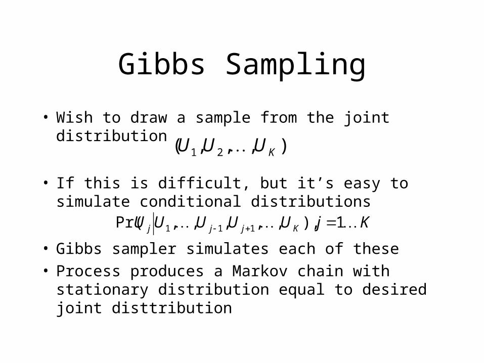
• Wish to draw a sample from the joint distribution
• If this is difficult, but it’s easy to simulate conditional distributions
• Gibbs sampler simulates each of these• Process produces a Markov chain with stationary
distribution equal to desired joint disttribution
),,,( 21 KUUU
KjUUUUU Kjjj 1 ),,,,,,Pr( 111
Algorithm 8.3: Gibbs Sampler
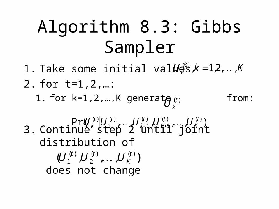
1. Take some initial values
2. for t=1,2,…:1. for k=1,2,…,K generate from:
3. Continue step 2 until joint distribution of
does not change
KkU k ,,2,1,)0(
)(tkU
),,,,,Pr( )()(1
)(1
)(1
)( tK
tk
tk
ttk UUUUU
),,,( )()(2
)(1
tK
tt UUU

Gibbs Sampling
• Only need to be able to sample from conditional distribution, but if it is known, then:
is a better estimate
M
mt
tlU klUu
mMu
k),|Pr(
)1(
1)(rP̂ )(
Gibbs sampling for mixtures
• Consider latent data from EM procedure to be another parameter:
• See algorithm (next slide), same as EM except sample instead of maximize
• Additional steps can be added to include other informative priors
),( MZ
Algorithm 8.4: Gibbs sampling for mixtures
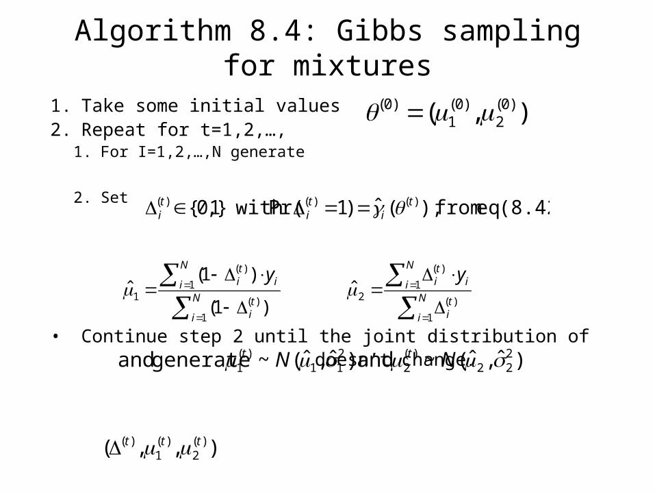
1. Take some initial values2. Repeat for t=1,2,…,
1. For I=1,2,…,N generate
2. Set
• Continue step 2 until the joint distribution of doesn’t change.
),( )0(2
)0(1
)0(
(8.42) eq from ),(ˆ)1Pr( with }1,0{ )()()( ti
ti
ti
N
i
ti
N
i iti y
1
)(
1
)(
1)1(
)1(̂
N
i
ti
N
i iti y
1
)(
1
)(
2̂
)ˆ,ˆ(~ and )ˆ,ˆ(~ generate and 222
)(2
211
)(1 NN tt
),,( )(2
)(1
)( ttt

Figure 8.8: Gibbs Sampling from Mixtures
Simplified case with fixed variances and mixing proportion
Outline
• 8.6 MCMC for Sampling from the Posterior
• 8.7 Bagging– 8.7.1 Examples: Trees with Simulated Data
• 8.8 Model Averaging and Stacking
• 8.9 Stochastic Search: Bumping
8.7 Bagging
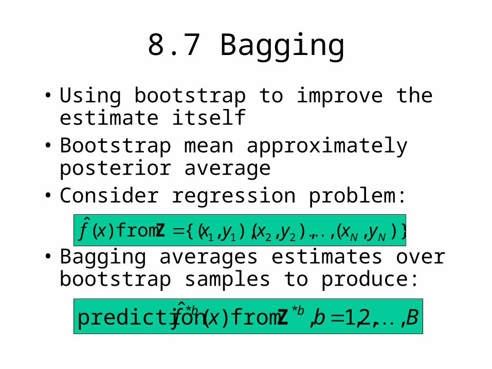
• Using bootstrap to improve the estimate itself
• Bootstrap mean approximately posterior average
• Consider regression problem:
• Bagging averages estimates over bootstrap samples to produce:
)},(,),,(),,{( from )(ˆ2211 NN yxyxyxxf Z
Bbxf bb ,,2,1, from )(ˆ prediction ** Z
Bagging, cnt’d
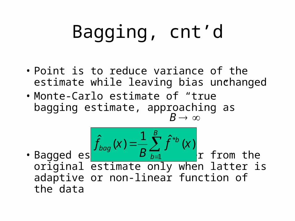
• Point is to reduce variance of the estimate while leaving bias unchanged
• Monte-Carlo estimate of “true” bagging estimate, approaching as
• Bagged estimate will differ from the original estimate only when latter is adaptive or non-linear function of the data
B
B
b
bbag xf
Bxf
1
* )(ˆ1)(ˆ
Bagging B-Spline Example
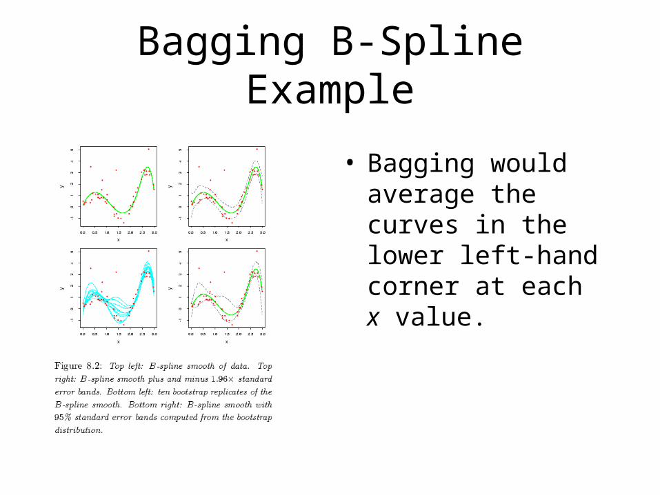
• Bagging would average the curves in the lower left-hand corner at each x value.
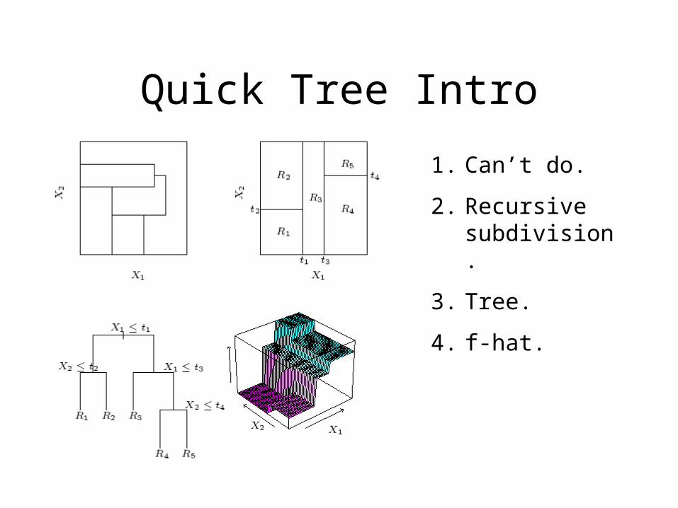
Quick Tree Intro
1. Can’t do.
2. Recursive subdivision.
3. Tree.
4. f-hat.

Spam Example
Bagging Trees
• Each run produces different trees
• Each tree may have different terminal nodes
• Bagged estimate is the average prediction at x from the B trees. Prediction can be a 0/1 indicator function, in which case bagging gives a pk proportion of trees predicting class k at x.

8.7.1: Example Trees with Simulated Data
•Original and 5 bootstrap-grown trees
•Two classes, five features, Gaussian distribution
•Y from
•Bayes error 0.2
•Trees fit to 200 bootstrap samples
8.0)5.0|1Pr(
,2.0)5.0|1Pr(
1
1
xY
xY
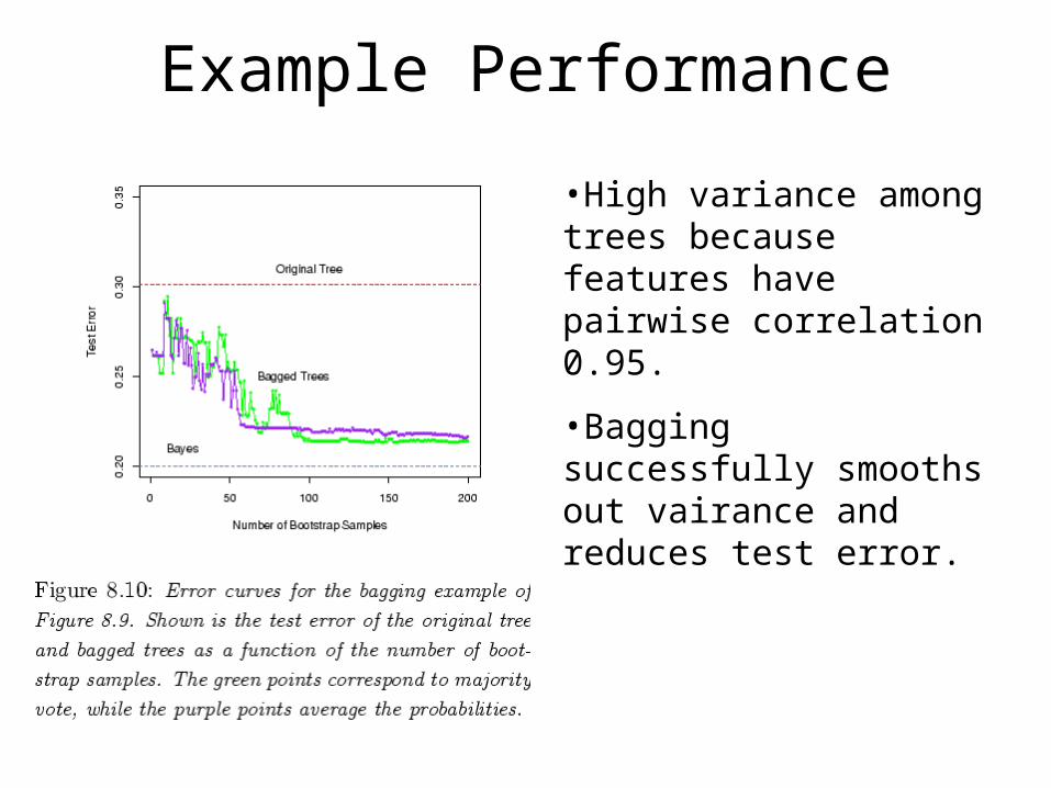
Example Performance
•High variance among trees because features have pairwise correlation 0.95.
•Bagging successfully smooths out vairance and reduces test error.

Where Bagging Doesn’t Help
•Classifier is a single axis-oriented split.
•Split is chosen along either x1 or x2 in order to minimize training error.
•Boosting is shown on the right.
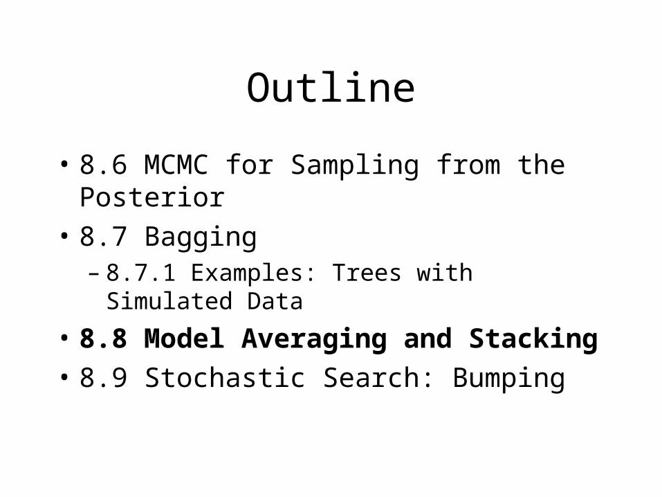
Outline
• 8.6 MCMC for Sampling from the Posterior
• 8.7 Bagging– 8.7.1 Examples: Trees with Simulated Data
• 8.8 Model Averaging and Stacking
• 8.9 Stochastic Search: Bumping
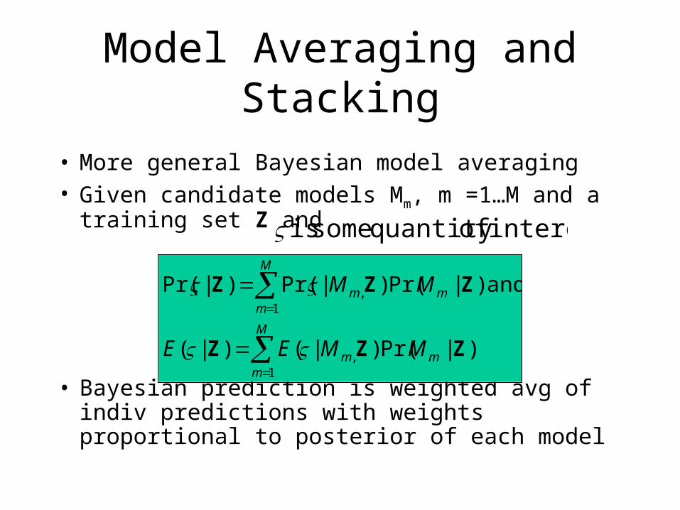
Model Averaging and Stacking
• More general Bayesian model averaging• Given candidate models Mm, m =1…M and a training
set Z and
• Bayesian prediction is weighted avg of indiv predictions with weights proportional to posterior of each model
)|Pr()|()|(
and )|Pr()|Pr()|Pr(
,1
,1
ZZZ
ZZZ
mm
M
m
mm
M
m
MMEE
MM
interest ofquantity some is
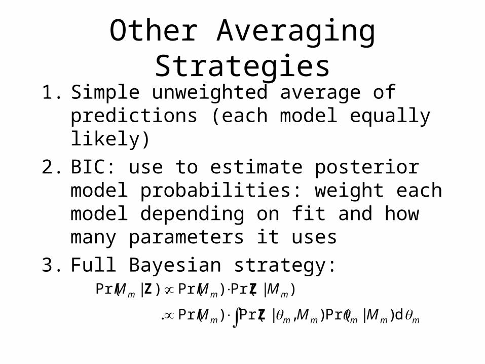
Other Averaging Strategies
1. Simple unweighted average of predictions (each model equally likely)
2. BIC: use to estimate posterior model probabilities: weight each model depending on fit and how many parameters it uses
3. Full Bayesian strategy:
mmmmmm
mmm
MMM
MMM
d)|Pr(),|Pr()Pr(.
)|Pr()Pr().|Pr(
Z
ZZ
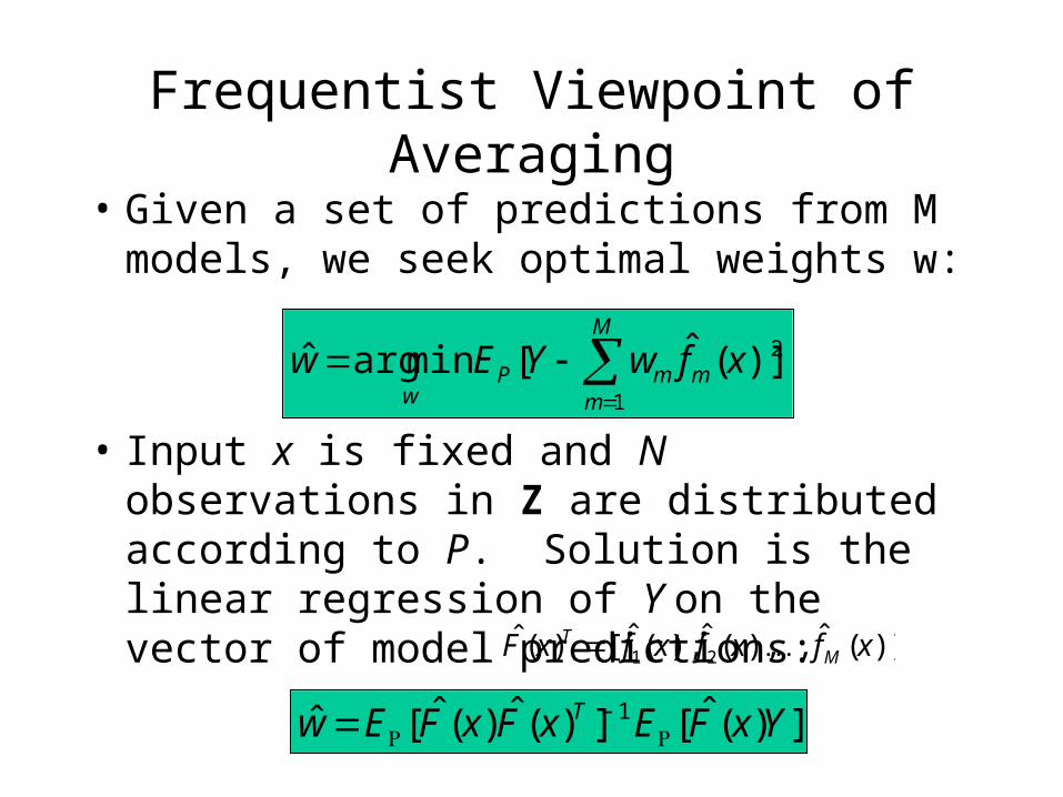
Frequentist Viewpoint of Averaging
• Given a set of predictions from M models, we seek optimal weights w:
• Input x is fixed and N observations in Z are distributed according to P. Solution is the linear regression of Y on the vector of model predictions:
M
mmmΡ
wxfwYEw
1
2)](ˆ[minargˆ
)](ˆ,),(ˆ),(ˆ[)(ˆ21 xfxfxfxF M
T
])(ˆ[])(ˆ)(ˆ[ˆ 1 YxFExFxFEw T
Notes of Frequentist Viewpoint
• At the population level, adding models with arbitrary weights can only help.
• But the population is, of course, not available
• Regression over training set can be used, but this may not be ideal: model complexity not taken into account…
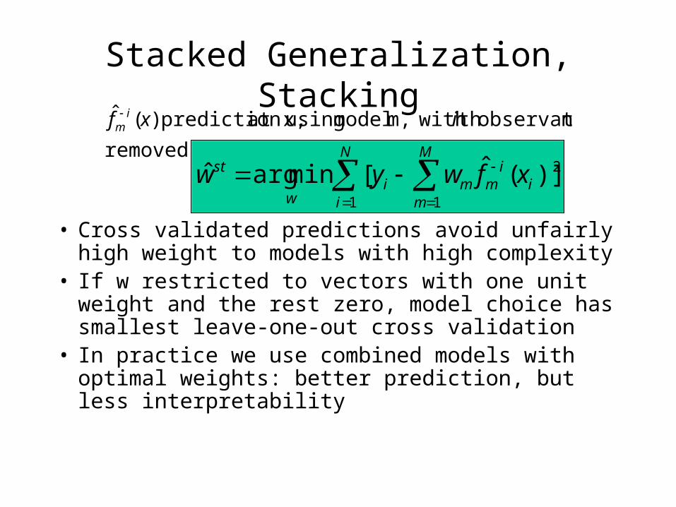
Stacked Generalization, Stacking
• Cross validated predictions avoid unfairly high weight to models with high complexity
• If w restricted to vectors with one unit weight and the rest zero, model choice has smallest leave-one-out cross validation
• In practice we use combined models with optimal weights: better prediction, but less interpretability
removed.
nobservatioth with m, model using at x, prediction )(ˆ ixf im
2
1 1
)](ˆ[minargˆ ii
m
N
i
M
mmi
w
st xfwyw

Outline
• 8.6 MCMC for Sampling from the Posterior
• 8.7 Bagging– 8.7.1 Examples: Trees with Simulated Data
• 8.8 Model Averaging and Stacking
• 8.9 Stochastic Search: Bumping
Stochastic Search: Bumping
• Rather than average models, try to find a better single model.
• Good for avoiding local minima in the fitting method.
• Like bagging, draw bootstrap samples and fit model to each, but choose model that best fits the training data
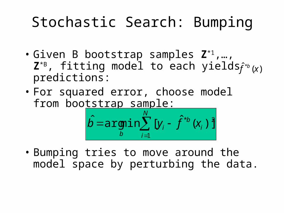
Stochastic Search: Bumping
• Given B bootstrap samples Z*1,…, Z*B, fitting model to each yields predictions:
• For squared error, choose model from bootstrap sample:
• Bumping tries to move around the model space by perturbing the data.
)(ˆ * xf b
2*
1
)](ˆ[minargˆi
bN
ii
bxfyb

A contrived case where bumping helps
•Greedy tree-based algorithm tries to split on each dimension separately, first one, then the other.
•Bumping stumbles upon the right answer.