endliliiip. no lnn ilk
TRANSCRIPT

AADA 99 HYDROLOGIC ENGINEERING CENTER DAVIS CA F/G 8AVR COMPUTER MODELS FOR RAINFALL-RUNOFF AND RIVER HyrJRAULIC ANALYETS~ l
ACOSIFIED HEC-TP-3 NL
ENDLILIIIP.
- " ""I"
nO lnn ilK
771-11

MARCH 1913
VTECHNICAL PAPER NO. 35
COMPUTER MODELS FORRAINFALL-RUNOFF AND
RIVER HYDRAULIC ANALYSIS
byDARRYL WODAVIS
DT1C
IDC>,
'It THE HYDROLOGIC
*research
-training
CORPS OF ENGINEERS PU. S. ARMY
AjI

Papers in this series have resulted from technical activities of TheHydrologic Engineering Center. Versions of some of these have been publishedin technical Journals or in conference proceedings. The purpose of thisseries is to make the information available for use in the Center's trainingprogram and for distribution within the Corps of Engineers.
I7

UNCLASSIFIEDSECURITY CLASSIFICATION OFTo AG lhn Date Entered)
REPOT DCUMNTATON AGEREAD INSTRUCTIONSREPOT DCUMNTATON AGEBEFORE COMPLETING FORM
REPORT NUMBER 2. GOVT ACCESSION No. 3. RECIPIENT'S CATALOG NUMBERTechinical aperjo0.35 _________________
4- 'rTt jE f S. TYPE OF REPORT & PERIOD COVERED
WI 1TER ,_= ELS FOR P INFALL-,JJNOFF A NID, IVER 6 E F R I G O G E O T N M EO~AULI CANALYSI Is"''6 EROMN R. EOTNME
- AUTHOR(&) 8. CONTRACT OR GRANT NUMBER(&)
IA0 RRYL4./DAVIS
9. PERFORMING ORGANIZATION NAME AND ADDRESS 10. PROGRAM ELEMENT. PROJ91T, TASK
US Amy C rp of nginersAREA & WORK UNIT NUMBERS
The Hydrologic Engineering Center609 Second Street, Davis, CA951
II1 CON TROLLING OFFICE NAME AND ADDRESS 12. REPORT DATE
13. NUMBER OFA
_____________________________________________ /IA14. MONITORING AGENCY NAME & ADORESS(ff different from Controllingl Office) IS. SECURITY CLASS. (of fti report)
AnclassifiedISa. DECL ASSI FICATION/ DOWN GRADING
SCHEDULE
16. DISTRI13UTION STATEMENT (of this Report)
fistrihution of this nublication is unlimited.
17. DISTRIBUTION STATEMENT (of the abstract entered In Block 20. if different from Report)
18. SUPPLEMENTARY NOTES
Presented at the Snrinn 1973 Conference of the Civil EngineeringProrran Ap~plications (CEPA) Conference, San Francisco, California
19. K(EY WORDS (Continu~e on reverae side if necessary and identify by block number)
Hydroloqic model, hydraulic model, river hydraulics, computer application.
,) 4bTRACT (Continue on reverse sicip It nocesmy and tdenff 4' by blocknmbr
The avnolication of computer technolopy to anal ' sis of the rainfall-runoffprocess and the hydraulics of natural rivers has greatly expanded in the pastfew Years. A large number of special purpose programs and a few programs
nqineerSE URblms CLAheIC Hyrloi Eniern PAGEe (W.n hasa dentlrpdd

UNCLASSIFIEDSECURITY CLASSIFICATION OF THIS PAGEWMhan Data Entered)
20(Continued)Enaineerinn Center and discusses the capabilities of two of these programs:(1) Flood Hydrograph Package (HEC-l) and (2) Water Surface Profiles (HEC-2)
Acc,ssion For
MTIS GRA&IDTIC TAIRIUn.n n oan c ed --I
Just if ic -t i.n . .
By - -Dist ri but i o:;/Availability C~des-
Dist Special
SECURITY CLASSIFI(CATION OF THIS PAGE(nen Data Entered)
. . . . . , . . .. . . . . .
a- - -- -- ~ ----------

COMPUTER MODELS FOR RAINFALL-RUNOFF
AND RIVER HYDRAULIC ANALYSIS1
by
Darryl W. Davis2
INTRODUCTION
The application of computer technology to analysis of the rainfall-
runoff process and the hydraulics of natural rivers has greatly expanded
in the past few years. A large number of special purpose programs and
a few programs designed for general application have been developed and
applied to hydrologic engineering problems. The Hydrologic Engineering
Center (HEC) has developed, over the past 8 years, a number of generalized
computer programs for use by the US Army Corps of Engineers in analyzing
hydrologic engineering problems. This paper briefly describes the
activities of The Hydrologic Engineering Center and discusses the capa-
bilities of two of these programs: (1) Flood Hydrograph Package (REC-l)
and (2) Water Surface Profiles (HEC-2).
THE HYDROLOGIC ENGINEERING CENTER
The Hydrologic Engineering Center, established in 1964, has three
principal missions: (a) conduct research and development of hydrologic
engineering techniques for use in the Corps' day-to-day work, (b) provide
training for Corps of Engineers employees in traditional as well as newly
IFor presentation at the Spring 1973 Conference of the Civil EngineeringProgram Applications (CEPA) Conference, San Francisco, California
2Civjl Engineer, The Hydrologic Engineering Center, Davis, California
J"P

developed hydrologic engineering techniques, and (c) provide assistance
to Corps field offices in hydrologic engineering studies. The Center
has recently been assigned responsibility in the area of planning
analysis so that its capabilities in the field of systems analysis can be
focused on priority components of planning problems. From the beginning,
HEC concentrated on computer applications and utilization in carrying
out each of these missions (reference 1).
The research and development work has resulted in the coding, testing
and documentation of about 30 generalized computer programs in hydrologic
engineering. The programs are generalized in that they can be applied
without modification to almost any problem in their specific area of appli-
cation regardless of the scope of the problem, the geographic location of
the problem, or the degree of detail required in a particular solution.
Five of the programs are large programs that combine a number of functions
into a single package. These five programs are in the areas of flood
hydrograph analysis, water surface profiles, reservoir systems analysis
for flood control and conservation and monthly streamflow simulation.
The training activities conducted or sponsored by the Center are
designed to improve the hydrologic engineering capabilities of the Corps
of Engineers in accomplishing its civil works mission. This specialized
training contributes to more efficient performance of technical studies
associated with the planning, design and operation of civil works projects.
The training program includes about 20 weeks per year of I- and 2-week
2
-, -I

courses with classroom instruction in topics of hydrologic engineering.
Individual training and short seminars are also included when desirable.
The special assistance mission of the Center serves to point up the
needs for training as well as for research and provides realistic problems
for testing techniques and programs.
THE FLOOD HYDROGRAPH PACKAGE (HEC-l)
General Capabilities
HEC-l can be characterized as a single storm event flood runoff
simulation model. Most ordinary flood hydrograph computations associated
with precipitation and runoff on a complex multisubbasin, multichannel
river basin can be accomplished with the program. Because of the modelling
capability of the program, a number of other routines Pre included that can
assist in determining the appropriate parameters needed to model the runoff
process and to evaluate the effect of management alternatives.
The five major types of computations that can be performed by HEC-1
are:
" Generalized precipitation, runoff, routing and combining
operations to simulate the hydrologic response of a
watershed and its stream network (the modelling element);
" Optimization of routing parameters (assistance in parameter
derivation)
" Optimization of unit hydrograph and loss rate parameters
(assistance in parameter derivation);
-.... -. " 4 . .

" Stream system computations for specified precipitation
depth-area storm relationships for the entire watershed or
region (application of modelling capability);
" Specialized precipitation streamflow network simulation
relative to multiple floods for multiple plans of basin
development and the economic analysis of flood damages
(evaluation of management alternatives).
In the process of modelling a basin, the program provides several
techniques for inputting and distributing the precipitation, treating
the precipitation as rainfall or snowfall, computing rainfall and snow-
melt losses and excess, determining subbasin outflow hydrographs from unit
graph techniques, and routing hydrographs by storage routing methods. If
necessary, different techniques for each process may be combined in the
same job for the basin being modelled. Graphical display of intermediate
or summary hydrographs and precipitation can be produced where desired.
The program may be used to optimize specified parameters of the precipi-
tation runoff or routing processes for a stream reach or subbasin to achieve
a best-fit with respect to an observed hydrograph and known precipitation
or a known inflow hydrograph.
The precipitation depth-area stream system computation is designed to
compute a consistent hydrograph at all desired points in a complex basin so
that each corresponds to a specific depth-area relationship. The procedure
operates by computing simultaneously a maximum of five base floods, each
4

representing average rainfall intensity corresponding to a specified
area size. An interpolated hydrograph is automatically established for
each concentration point based on the size of the area tributary to that
point. This routine is useful in stream systems or in urban storm
drainage computations where it is desired to compute a number of synthetic
events (such as a 100-year flood) at a large number of locations.
The routine for evaluating reservoir and channel development plans
for one or more locations includes the computation of average annual
dollar benefits at each damage center for each plan of development as well
as for existing conditions. This involves simultaneously computing a number
of system floods for each plan, covering the entire range of floods that
significantly contribute to damages. The floods may be either multiples of
the runoff from a single representative storm or the runoff from multiples
of a typical storm rainfall pattern. Flow-damage relations for each type
of damage and flood-peak frequency relations for existing conditions must
be specified for each damage center. Unit hydrograph coefficients, loss
coefficients, degree of imperviousness and routIng coefficients for each
plan must also be specified.
Modelling Rainfall-Runoff with HEC-I
The program is designed to simulate the storm rainfall-runoff
process and is composed of the appropriate mathematical relationships and
constants that describe the response of the watershed to rainfall. The
model accepts total storm rainfall for each subbasin, deducts losses to
determine rainfall excess, transforms the excess to streamflow by the
-- - -. w . . .
_ . n n

unit hydrograph technique, and translates the streamflow through valley
storage and reservoir storage by simple routing procedures.
Modelling a complex basin consists of defining its topologic structure
(subbasin boundaries and areas, stream channels and the logical relation-
ships between the subbasins and stream channels), and defining the parameters
that describe the rainfall-runoff response of the subbasins and channels
of the river basin. Parameters are needed to determine: (1) basin average
total precipitation and its time distribution for each subbasin, (2) precipi-
tation loss rates for selected storm events, (3) unit hydrographs for each
subbasin, (4) base flow controls for each subbasin, and (5) routing criteria
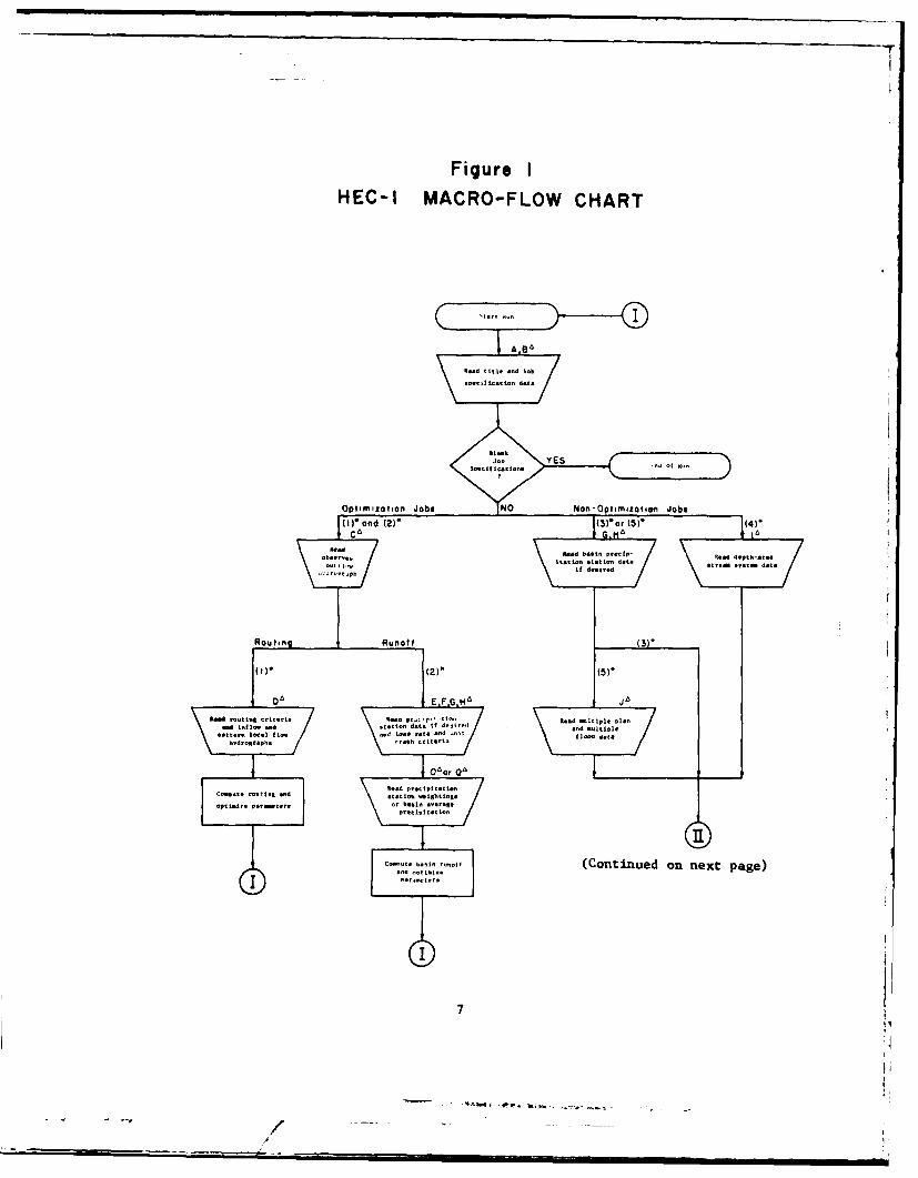
for each channel reach. The detailed computational algorithms can be found
in reference 2. Figure 1 is a simplified flow chart of HEC-l.
Topology. The topology of the basin is described in the program
essentially by the way the sequences of operations are specified. Hydrographs
are computed, routed and combined with other hydrographs in accordance with
the data sequence provided. In this manner any complex basin consisting of
a very large number of subbasins and routing reaches can be accurately described.
Precipitation. The precipitation applied to a subarea for runoff compu-
tations may be determined by three methods. The computed precipitation will
then be treated as rainfall or snowfall depending upon temperature criteria.
a. Subbasin total precipitation is computed from nonrecording
station precipitation according to weights provided for each station. The
subbasin total precipitation can also be computed considering longer term
weighting values such as normal annual amounts that may reflect consistent
6
-T
Figure IHEC-I MACRO-FLOW CHART
Y S e- ofNteOlf Icat tong Jobs
Optimization Jobs O Non-OptwmizotsOfi Jobs
(onf (2)* (W or (5)* (4)',,,..° - I<,o ( .1Ilat c G.K"
oaid b.t Proip- Red depth-
00' L,,o if d d *tren syst. data71 if a..tb
Routinq Runoff (3
111"(21) (51)
DA E.F.G.H
gad oatfltrtoiIt.t*a ',, ti-Rad .ltiplit 1110aud inline and ation data if d andpartt,-noni fi- n :n1 ia ito and uit flod dtd
h~~d f~llllmhd er on liita tlod ol1 1oo°0,ooC:"., \ -/ .....C t. rootin .and *itllin a itinga
aOlfill Panator. or basin avrag:*Vr,"iitat ion
basin runoff (Continued on next page)
C t
,aarfr
- - "d¢1

IO
ReaCPLrd10
Subarea runoff Routing Combining Balancin Cons arin Summary(11* Ell -87) (Be], C951 E991
,..I- Pre .l at r.?. Combie peatouey ee ea., R0
eec*rotttat it ad atal lv,. tdrogfaphe rcO t. h~aO lttteah atr::. netor
tot ctti tt~e*tot I f ow
Crimper Co.r ceotpuCome
Rot nsHd'.oerah hydrograsft
IsI
Rate -- IRt e Cl ruIIRCORO13d flooda~ ~eafo ngr ~.taa~e
paaehe R e th asag intdcate te v:Ia % fo p v ar iablot OPR w-a hich t 1 . Rhchet08.1 he Nhe card deb le* t"*. ao t j pete be It. - aea7e
03) 001eeaf Srafff ...-harfl aton
Ii) 00 0 : Ai a Sore S rh Sytsc1 t em ri o , r a t i e
(2- ?! Combhiss IC" hydraegoaph.r at thin station
951OcWeee ecatoed Met obweaved Irdegreph, aR tis otiation
=4I end elj-piit ee ry Imforttem
physiographic effects in the subbasin. The subbasin-mean recording
precipitation pattern (time distribution) is computed in a similar
manner with station weights as appropriate. The subbasin-mean precipita-
tion distribution (time distribution of total storm rainfall) is then
computed using the relative pattern to distribute the total subbasin
rainfall.
b. Known temporal and spatial precipitation for a subbasin can
be supplied directly. By this method precipitation can be supplied
for each interval or as a time pattern for a given storm total. Precipita-
tion distributions may also be specified for two differently sized areas and
the program will perform a logarithmic interpolation of the two patterns
for a specified area.
c. The program provides for automatic computation of standard
project storm (SPS) precipitation using Corps of Engineers criteria and
for probable maximum precipitation using criteriq developed by the National
Weather Service. For the SPS, the largest day of'precipitation is preceded
by the second largest and followed by the third largest. Six-hour storm
amounts within each day are similarly distributed. A storm transposition
coefficient can be supplied or will be computed by the program as a default
option.
Where snowfall and snowmelt are considered, there is provision for
separate computation in up to ten elevation zones. These zones are usually
considered to be in elevation increments of 1,000 feet, but any equal
increments of elevation can be used as long as the air temperature lapse
9

rate corresponds to the change in elevation within the zone. The input
temperature data are those corresponding to the bottom of the lowest
elevation zone. Temperatures are reduced by the lapse rate in degrees
per increment of elevation zone. The base temperature at which melt will
occur must be specified because variations from 320F (0°0 might be
warranted considering both spatial and temporal fluctuations of temperature
within the zone.
Precipitation is assumed to fall as snow if the zone temperature is
less than the base temperature plus 2 degrees. Melt occurs when the
temperature is equal to or greater than the base temperature. Snowmelt
is subtracted and snowfall is added to the snowpack in each zone. Snow-
melt may be computed by the degree-day or energy-budget methods.
Precipitation Loss Rates. Loss rates can be computed using initial
and uniform losses or by a function which relates loss rates to rainfall
and snowmelt intensity and to accumulated loss (ground wetness). Figure 2
shows the loss rate function for a snow-free basin. The loss rate function
is successively applied for each computational interval.
The loss rate parameters of figure 2 are:
DLTKR - Amount of initial accumulated rain loss during which
the loss rate coefficient is increased. This param-
eter is considered to be a function primarily of
antecedent soil moisture deficiency and is usually
different for different storms.
10
4 -

STRKR - Starting value of loss coefficient on exponential reces-
sion curve for rain losses (snow-free ground). The
starting value is considered a function of infiltration
capacity and thus depends on such basin characteristics
as soil type, land use and vegetal cover.
RTIOL - Ratio of rain loss coefficient on exponential loss curve
to that corresponding to 10 inches more of accumulated
loss. This variable may be considered a function of the
ability of the surface of a basin to absorb precipitation
and should be reasonably constant for large rather
homogeneous areas.
ERAIN - Exponent of precipitation for rain loss function
ALOSS - (AK + DLTK) PRCPERAIN
that reflects the influence of precipitation rate on
basin-average loss characteristics. It reflects the
manner in which storms occur within an area and may be
considered a characteristic of a particular region.
Varies from 0.0 to 1.0. The terms in the equation are
defined as:
ALOSS = loss rate for particular time interval
11
4- --~ - -,,..*--- - -

AK M loss rate coefficient at beginning of time
interval, value on STRKR exponential loss
curve.
PRCP - rainfall intensity in inches (mm) per hour.
DLTK - incremental increase in loss rate coefficient.
DLTK is assumed to be a parabolic function of
the accumulated loss for DLTKR amount of
accumulated loss. DLTK is a maximum of 0.2
DLTKR initially reducing to zero when the
accumulated loss equals DLTKR.
12
U --12

Unit Hydrograph. The unit hydrograph corresponding to the
appropriate duration of rainfall excess can be supplied directly or may
be computed from coefficients of two synthetic techniques; the Clark
procedure and the Snyder procedure. The Clark procedure develops a
unit hydrograph from a coefficient describing the subbasin time of
concentration and a coefficient describing the subbasin natural storage
characteristics. A time-area diagram (sometimes termed a time delay histo-
gram or translation hydrograph) with a base time equal to the time of
concentration is routed through a linear reservoir characterized by
the storage coefficient. The time-area relation may be derived from
subbasin physiographic data and supplied directly or the program may
be permitted to compute and use an idealized relationship that consists
of a simple reverse parabola symmetrical about the center of the time
base.
If a unit hydrograph that conforms to specified Snyder coefficients
is desired, it is established by successive approximations for the corres-
ponding Clark coefficients.
Base Flow and Recession. The program assumes that the flood to be
computed occurs after a previous flood and therefore begins at a flow
on the recession limb of the previous flood hydrograph. The recession
is assumed to be described by &, exponential function. The parameters
required to describe the base flow and recession are the starting flow,
the flow at which recession begins, and the recession constant. Figure
3 shows the base flow separation concept used by the program.
13
r --- ~ --

0.2 DLTKR DLTK: 0.2 DLTKRE [i( CUML/DLTXR)]2
A K S TRK R/RTIOL(0.I CI.ML)
RTIOL: A/B
01
a:
0
Arithmetic Scale
ACCUMULATED LOSS (CUML) -inches (mm)
A LO SS = (AK+ D LTK)PRCPERAINFig. 2. General Loss Rate Function on Snow-Free Ground
DirectSurfaceRunoff
0 Recession Threshold
TIME
Fig. 3. Base Flow Separation

T
Routing. The routing procedures available in the program are the
simplified storage routing procedures that neglect inertia effects.
All these procedures can be used for etreamflow routing and a few are
useful for simple reservoir routing.
The Huskingum procedure determines reach outflow based on inflow and
coefficients describing the reach travel time and attenuation character-
istics. The Tatum method is a simplification of the Muskingum procedure.
The modified Puls (sometimes termed storage indication) is simply a solution
of the continuity equation when storage and outflow are uniquely related
and is appropriate for both streamflow and simple reservoirs. The time-
of-storage procedure is primarily a simple reservoir procedure and the
working R and D is a combination of the Muskingum technique and the
modified Puls procedure. The straddle-stagger technique, a strictly
empirical procedure, is also included.
Automatic Derivation of Parameters
HEC-l can derive loss rate and unit hydrograph coefficients or
routing coefficients automatically. In order to optimize coefficients,
a hydrograph of observed runoff must be supplied. In the case of routing
optimization, a pattern hydrograph for intermediate runoff (between given
inflow and outflow) must also be supplied. This pattern hydrograph is
automatically multiplied by a ratio to make the volume of intermediate
runoff equal the difference between inflow and outflow volumes.
Coefficients are derived by successive approximations to determine the
optimum values of a set of variables that will result in a minimum value of an
15
-r ------. -...

-r
objective function. The objective function for optimal reconstitution
is the weighted root-mean-square errors between computed and observed
flows. In order to improve the reproduction of peak flows, errors
associated with high flows are weighted heavier than those associated
with low flows. Each error square is multiplied by (Q + Q)/2Q where
& is the average flow. A volume check is included in the hydrograph
reconstruction to assure approximate correspondence in volume between
the observed and computed hydrographs.
The optimization process terminates after a specified number of steps.
If a reproduction is not satisfactory, considerable improvement can be made
in a second run by a routine that temporarily distorts the observed hydro-
graph to torce a better reproduction without impairing the validity of the
results. For example, if a portion of a reconstituted hydrograph is too
low, it can be fitted better by increasing a key flow by about double the
discrepancy. These temporary adjustments to the flow are removed before
the hydrograph is printed.
lydrograph Balancing
A hydrograph balance routine is included to convert any given hydro-
graph to one having specified volumes within given durations. Starting
with the shortest duration specified, the period of maximum flow of the
given hydrograph is determined, and the sum of all flows (t)'t have not
already been used in shorter-duration computation) within each period is
computed. Flows are adjusted within each period by multiplying by the ratio
16

required to obtain the incremental volume needed. Since the changed
shape of the hydrograph can alter the location of maximum flows, this
process is repeated until all volumes are within 1 percent, using
the derived hydrograph as the new pattern hydrograph each
iteration.
General Input Structure
HEC-l is designed to accept input in card form that will describe
the type of job to be performed, its scope and the detailed information
required for processing.
A single job to be processed by HEC-l consists of one set of A
through J cards followed by repeated sets of K cards through Z cards
as necessary. There are five types of jobs that can be processed by
HEC-l, and these are specified by a key variable.
The values of key variables determine the data to be processed. Only
the cards required for the desired process are to be used, and they must
be in the proper sequence.
Cards K through Z are used to specify the data relative to the individual
subarea, routing reach, or combining operations and economic analyses. The
order of computing hydrographs is vital in certain respects since the most
recently computed hydrographs remaining in storage are the ones that may be
combined or routed.
17
- /1'

-T
The type of information contained on the data cards is summarized below:
Card Code Description
A Job title
B Job specifications
C Observed hydrograph to be reconstituted
D Routing optimization criteria and observedinflow hydrograph
E, F Unit graph and loss rate optimization criteria
G, H Station precipitation data for all subbasinsof the watershed
I Precipitation depth-drainage area data
J Multiflood, multiplan data
K Computation specification for model building
L Hydrograph balancing criteria
M-X Subarea runoff computation data including pre-cipitation, losses, and unit graph information
Y Individual reach routing criteria
Z Economic and flood frequency data
In modelling a watershed (nonoptimization jobs) the K cards, followed
by the appropriate runoff or routing cards, will be repeated as many times
as necessary in order to compute the runoff, routing and combining of hydro-
graphs in a logical progression through the basin.
An example of program input and output for a subarea runoff hydrograph
computation is contained on the following pages.
18
--.. ' ' 7 . - - - - - - - - - - - -_i | I

ItI
a.~~~ v) I ' qr yc
w I I II
In o 1, 1- 1
o w,- 4, c ... n
x- I-) 2 -Az )1
IL w oll< I "
-1 •j z v. •c r •••o,
DO) c o, y. C- c: :>
I u
-I - ( 5-
I. N. C. M) C,
Coo -I 1
19
I
0 1 I
I
..* . . . •... . . . . . . . . . . e . e . . .
IiI
I I
cc, 0 .
*, a,
I I 0
N3 CL
ic f T d r I 1 LI -V,
I 0

I I . . . . .. . . . . . . . . . . . . . . .
° 1 ItII I
................. ........ . .... ........
I I , J 4
.......... . . . .. . . . ..... ........................
1 JI I
. . . ,
.. . .I
* . I I• '
1) C, C;0
0t W, -0 1 cGNI. pc
3. m' YNc 1 ~ I r 0 r 0 09 ' WD 'aaf
*il' 1 I
I .. .. . I
I i I I+ !
' , ' I.
I I
0 .• • • ° •
210
.OoCo .. ... ,iOOC. C' c O0' o t.) I 't3 OL .. ..,C(.. .., [ ..
*
I
"--. /, -- _-

Hardware and Software Requirements
HEC-1 has been developed and tested primarily on the UNIVAC 1108
and the Control Data Corporation 6600 computer systems. It was then
adapted for use on the GE 400 series computers. The program is written
in FORTRAN IV and contains about 3,000 FORTRAN statements. Table 1
shows the hardware requirements and selected running times for the pro-
gram.
Table 1. Hardware Requirements and Running Times
FORTRA1 IV CompilerFour tape and/or disk units*
UNIVAC 1108 CDC 7600 GE 400
Memory (words) 38,700 35,400 32,000
Printer (positions) 132 132 120
Compilation (CPU seconds) 30 3 --
Execution of Test 5(CPU seconds) 11 1
*May only require two tapes or disks if output hydrographs are not to be
saved or read in from previous jobs.
WATER SURFACE PROFILES (HEC-2)
General Capabilities
HEC-2 has been designed to perform steady gradually varied flow pro-
file computations for natural channels. The program accommodates local
obstructions such as weirs, culverts and bridges so that a continuous
(uninterrupted computation) profile can be computed for either subcritical
or supercritical flow. Reference 3 contains detailed information on the
capabilities and data preparation requirements.
22

Profile computations for channel reaches are based on solution of the
one-dimensional Bernoulli equation with energy loss due to friction
evaluated with the Manning's equation and other losses evaluated by appli-
cation of the shock-loss equation. The solution procedure used is
generally referred to as the standard-step method.
The flow field at a cross section is divided into main channel and
overbank areas and the overbank areas are subdivided to account or
nonuniform velocity distributions. The reach distances to adjacent cross-
sections may be specified for the channel and overbank areas.
Energy losses at obstructions can be accommodated by three alternative
means. The loss (rating curve) may be supplied directly. The "normal"
bridge routine evaluates energy losses by normal standard-step computations
with corrections for flow area and wetted perimeter. The "special" bridge
routine applies the principles of conservation of momentum to evaluate
depths and thus, indirectly, energy loss. It observes the hydraulic
control concept of critical depth in determining the flow characteristics.
This routine also computes energy losses based on the weir equation when
flow is over the road deck, and the orifice equation when flow is confined
to the bridge opening and under pressure. Bridge characteristics are
described by the natural valley cross section, the top of roadway and low
chord profiles, and appropriate discharge and loss coefficients.
The program has been carefully designed to ease data handling and
manipulation requirements. Many routines and options are available for
describing cross sections, specifying the portion of the cross section
23
..." ... --- - '- l "i.... . .../..
that is effective in passing flow, manipulating the cross section by
skewing and raising and lowering as desired. Utility features permit
processing many profiles during a single run, plotting output, summarizing
computations and editing data. A large number of diagnostic notes are
output during computations.
The program has a few special routines designed to assist in
flood plain management and flood insurance studies wherein encroach-
ments must be evaluated and floodways must be designated.
Computational Procedures for Channels
The standard-step method of computing water surface elevation at
specific locations requires a trial solution of the Bernoulli equation.
Figure 4 indicates a schematic of the computation procedure. The
terms in the equation that require special attention in natural
channels are the velocity head and the friction loss.
Velocity Head. Because the Bernoulli equation is one-dimensional,
the velocity head term must be corrected to account for the kinetic energy
content of the moving total fluid considering the nonuniformity of the
velocity distribution. The procedure used is to subdivide the cross
section at each coordinate point, compute the velocity head for each sub-
section and weight the incremental velocity head in accordance with the
discharge in each subsection. The velocity for each subsection is computed
by the Manning equation for the roughness and wetted perimeter of that
subsection.
24

Sip,
f W.SL
CHANK0
SECTION-202YFO -L
PROILE 2
Computation Procedure
Conditions are known @ 1
0 Assume water surface elevation ata - WSEL (2)
a*** Compute conveyance- K(2) - E K a+ K b+ *+ K
where: K -4- AR2/n
***Compute representative rate of friction loss
K -K~l) +K(22_ *s2av 2 av 2
K
e Compute WSEL(2) 2 aWSL() WELl 1 *6a 21 +c*IVz 2WSL2 -W2~l g + av- w +C 2g -2p
Compare and repeat until criterion met.
Fig. 4. Schematic of Computation Procedure
25

Friction Loss. The friction loss between adjacent cross sections is
computed as the product of the representative rate of friction loss
(friction slope) and the weighted reach length. The weighted reach length
is determined by weighting the channel length for each overbank area and
the main channel by the discharge flowing in each of these major section
elements. The representative rate of friction loss is determined by
averaging the conveyances of the adjacent cross section and then computing
an equivalent energy grade line slope from the Manning equation. The con-
veyance of each cross section is the sum of the conveyances of each subsection
within the cross section. The conveyance of each subsection is computed
from the geometric and hydraulic parameters of the Manning equation as
indicated in figure 4.
Other Losses. The program considers other losses to be expansion and
contraction losses that are generated because of changes in cross section
geometry. The loss is computed as the product of the appropriate loss
coefficient and the absolute value of the difference in velocity head.
The loss is computed each time a new cross section is encountered, including
those through bridges.
Critical Depth. The program assumes the profile being computed is
either all subcritical or all supercritical. Either can be processed but
must be done so separately. Critical depth therefore cannot be crossed
during a profile computation. If the search procedure determines that
the depth being computed lies on the other side of critical depth from the
initial specification, the program assumes critical depth at that
26

section, prints a note and proceeds to the next section. Critical depth
is calculated for every cross section for supercritical profiles but
only when necessary to determine if crossing is possible for subcritical
profiles. Critical depth is computed by a search procedure that seeks
the depth that results in the minimum value of specific energy. The
nonuniformity of velocity distribution in the cross section is considered
in th_ computations.
Comrutaiion Controls. The solution for critical depth and for the
water surface elevation at each cross section requires trial and error
iterative-type computations. The number of iterations used for each
computation is limited so that failure to converge would not cause profile
computation to cease. In those instances where convergence does not
occur, messages are generated to focus attention on problem areas. Failure
to converge is not necessarily caused by errors since complex natural
cross sections can give rise to inconsistencies in solution of the one-
dimensional equations.
Bridge Losses
Energy losses caused by structures such as bridges and culverts are
computed in two parts. First, the losses due to expansion and contraction
of the cross section on the upstream and downstream sides of the structure
are computed. Secondly, the loss through the structure itself is computed
by either the normal bridge routine or the special bridge routine.
Normal Bridge Routine. The normal routine handles the cross section
at the bridge just as it would any river cross section with the exception
27
C..- - -

that the area of the bridge below the water surface is subtracted from
the total area and the wetted perimeter is increased where the water
surface elevation exceeds the low chord. The bridge deck is described
by entering the elevation of the top of roadway and low chord, or by
specifying a table of roadway elevation and station and corresponding low
chord elevations. When only top-of-roadway and low chord elevations
are used, these elevations are extended horizontally until they intersect the
ground line. Pier losses are accounted for by the increased wetted peri-
meter of the piers. The normal routine is particularly applicable for
bridges without piers, bridges under high submergence, and for low flow
through circular and arch culverts. Whenever flow crosses critical
depth in a structure, the special bridge routine should be used. The
normal bridge is automatically used by the computer, even though data was
prepared for the special bridge routine, for bridges without piers and
under low flow control.
Special Bridge Routine. The special bridge routine can be used for
any bridge, but should be used for trapezoidal bridges with piers where low
flow controls, for pressure flow through circular or arch culverts, and
whenever flow passes through critical depth when going through the structure.
The special bridge routine computes losses through the structure for low
flow, weir flow and pressure flow or for any coubination of these. The
type of flow is determined by a series of comparisons as shown on figure 5
and as described below. First, the energy grade line elevations are
computed assuming alternately low flow and pressure flow control. The
28
/...

c *0
40~ :00
-j ai ce 0
U- c
0 c aV* .0 *
133A NI NOIIVA3-13 AOU3N3 E E 3IO C 0 I
0
0
z-zCa 0
00
0 0w Ci) w L
co z 1 L.tUn 0 0 -0A
01 p C . w 00 00
0WO 0 C
-1 0 j ISA.
29

higher energy grade line elevation determines the appropriate type of
flow. If pressure flow appears to control and the energy grade line is
above the minimum top-of-roadway elevation, then a combination of pressure
flow and weir flow exists. If the energy gradient is below the minimum
top of roadway, then pressure flow alone controls. If low flow appears to
control, and the corresponding energy gradient elevation is above the minimum
top-of-roadway elevation, then a combination of low flow under the bridge
and weir flow over the roadway approach exists; if the energy elevation
is below the minimum top-of-roadway, then low flow controls.
Low flow is further classified as Class A, B and C depending on whether
subcritical, critical, or supercritical flow occurs between bridge piers.
Class A flow (subcritical flow through bridge) is solved from Yarnell's
energy equation. Class B and C flows (critical and supercritical flows,
respectively) are handled by momentum relations which equate the momentum
flux at adjacent locations and solve for depth. The flow class (A, B or C)
is determined by comparison of the momentum flux within the constriction
based on upstream and downstream conditions and the momentum flux assuming
critical depth in the constriction. Weir flow is computed by the standard
broad-crested weir equation. The approach velocity is included by using
the energy grade line elevation in lieu of the upstream water surface
elevation for computing the head, I. Where submergence by tailwater exists,
the discharge coefficient is reduced by the computer program according
to a specified procedure. The total flow is computed by dividing the
weir flow into subsections, computing the incremental flow for each
subsection and summing all subareas.
30
F /
Pressure flow computations use the orifice flow equation with the
head defined as the difference between the energy gradient elevation
upstream and tailwater elevation downstream. The total loss coefficient
K, representing losses between the cross sections immediately upstream
and downstream of the bridge, is equal to the sum of loss coefficients
for intake, intermediate piers, friction, exit and other minor losses.
Often combinations of these three basic types of flow occur. In
these cases, a trial and error procedure is used with the equations
just described to determine the amount of each type of flow. The procedure
consists of assuming energy elevations and computing the total discharge
until the computed discharge equals, within one percent, the discharge
desired.
Program Input for Profile Computation
A major portion of the programming in HEC-2 is devoted to providing
a large variety of input and data manipulation options. The program
objective is quite simple--compute water surface elevations at all locations
of interest for given flow values. The data needed to perform those
computations include flow, starting elevation, cross section geometry and
roughness, and reach lengths. The options available for providing and
manipulating input are discussed in the following pages.
Flow. The river flow may be specified and altered in several ways.
The starting flow is normally specified as a single value when only one
flow is anticipated. If it is desired to use different flows for subsequent
jobs using the same cross sections, a discharge table may be used. The flow
31
may also be changed at any cross section such as at a confluence with
another river or stream. The flow change at any cross section becomes
permanent for subsequent cross sections. The flow for the entire profile
may be increased or decreased by a factor if desired. This feature
can be very useful in sensitivity studies.
Starting Elevation. The water surface elevation for the beginning
cross section may be specified in one of three ways: (1) as critical
depth ia which case it will be computed, (2) as a known elevation, (3) by
the slope area method. For beginning by the slope area method, the estimated
slope of the energy grade line must be provided and the initial estimate of
the water surface elevation is also needed. The flows computed for the
fixed slope and estimated depth are compared with the starting flow and
the initial depth is adjusted until the computed flow is within 1 percent
of the starting flow.
River Flow Geometry. Cross sections are required at representative
locations throughout the river reach. These are locations where changes
occur in slope, cross sectional area, or channel roughness; locations
where levees begin or end; and at bridges. In general, for rivers of
flat slope and fairly uniform section (drop of 3 or 4 feet per mile)
cross sections should be taken at least every mile. For steeper slopes and
very irregular cross sections, four or five cross sections per mile may
be necessary. Where an abrupt change occurs in the cross section, several
cross sections should be used to describe the change regardless of the
distance. Every effort should be made to obtain cross sections that
32
- ---- v 7 /

accurately represent the river geometry.
Each cross section in the reach is described by coordinates that
give a station number corresponding to the horizontal distance from
the first point on the left and the corresponding elevation of the
ground surface. Cross sections may be oriented looking either upstream
or downstream since the program considers the left side to be the lowest
station number and the right side the highest. The left and right
stations separating the channel from the overbank areas must be specified.
End points of a cross section that are too low (below the computed water
surface elevation) will automatically be extended vertically by the
program, if needed, and a message giving the vertical distance extended will
be printed.
There are times when the user wishes to use the previous cross
section as the current one (for uniform channels), with or without a modi-
fication, or to modify the current cross section (perhaps the surveyed
cross section is moved upstream or downstream). The horizontal dimensions
of the previous or current cross section can be increased or decreased
by a factor and all the elevations of the previous or current cross
sections can be raised or lowered by a constant.
The existing cross section can be modified due to the excavation of
a trapezoidal channel. The coordinate points are modified due to the
excavation, but no fill is used. The bank elevations and stations are
modified if the channel daylights outside the original bank stations.
If the alignment of the excavated channel is such that two separate
33
9~ ----- ----.. . .

channels exist, the division between overbank and channel will be based
on the excavated channel, and the old channel will be considered as
overbank (no fill). It may be necessary to change the reach lengths for
this case.
Levees require special consideration in comput.;.g water surface pro-
files because of possible overflow into areas outside the main channel.
Normally the computations are based on the assumption that all area below
the water surface elevation is effective in passing the discharge. How-
ever, if the water surface elevation is less than the top-of-levee
elevation, and if the water cannot enter the overbanks upstream or downstream
of that cross section, then all flow area in these overbanks should not be
used in the computations. By setting a code, the program will consider
only flow confined by the levees, unless the water surface elevation is
above the top of one or both sides of the levee, in which case flow area
or areas outside the levee will be included. It is important for the
user to study carefully the flow pattern of the river where levees exist
to determine such items as if a levee were open at both ends and flow
could pass behind the levee without overtopping it. Also, assumptions
regarding effective flow areas may change with changes in flow magnitude.
Where cross section elevations outside the levee are considerably lower
than the channel bottom, it may be necessary to confine the flow to the
channel.
Sometimes it is necessary to insert cross sections between those
specified because the change flow in characteristics between cross sections
34
/ . .... .. . . . .
is too great to accurately determine the energy losses. Up to three
interpolated cross sections will be generated between given cross sections
under certain conditions. It is possible to suppress program generated
interpolated cross sections, and they should be omitted when computing
several profiles on the same stream in order to use exactly the same
cross sections. The distance between cross sections used in the computation
can be specified for the left overbank, right overbank, and channel,
respectively. There are conditions where they will differ, such as at
river bends, or where the channel meanders considerably and the over-
banks are straight.
Channel Roughness. Since Manning's coefficient of roughness, n,
depends on such factors as type and amount of vegetation, channel
configuration and stage, several options are available to vary n. The
normal situation is when three n values are sufficient to describe the
channel and overbank roughness. Any of the n values may be permanently
changed at any cross section. Often three values are not enough to
adequately describe the lateral roughness variation in the overbanks in
which case up to 19 n values and corresponding cross section stations are
provided. The n values thus specified apply only to the overbanks, while
the value used for the channel is as nornally entered.
Data indicating the variation of Manning's n with river stage may
be used in the program. This option applies only to the channel area.
It is possible for subsequent runs of the same job to multiply the
n values specified by a multiplier. The desired multiplier is simply entered
for each job. This feature may be useful in calibration and sensitivity studies.
35
! ! m/

-r
Manning's n can be computed from known high water marks along the
river reach if the discharge, relative ratios of the n values for the
channel and overbanks and the water surface elevations at each cross
section are known. The "best estimate" of n for the first cross section
must be provided since it is not possible to compute an n value for
this cross section. The relative ratio of n between channel and over-
bank is set by the first cross section and will be used for all subsequent
cross sections unless changed. The n values required to match the high water
marks are then computed provided an adverse slope in energy grade line
is not encountered, in which case computations restart using n values
from the previous section.
Utility Features and Output
Several profiles may be computed using the same cross section data.
A summary printout will provide a concise listing of the key results for
all profiles for each cross section. The user may select a number of the
variables to be retained for the summary printout.
Multiple Stream Profiles. The water surface profile computations
may be extended up both forks of a river or throughout a whole river basin
for single or multiple profiles in a single computer run. The profile is
first computed for reach 1 from the most down.itream point to the end of
one tributary. The data for a second tributary (reach 2), whose starting
water surface elevation was determined when reach 1 was calculated,
follows the data for reach I. When a negative section number is
encountered, the program will search its memory for the computed water
36

surface elevation that corresponds to the negative section number. It
will then start computing the profile for reach 2 with the previously
determined water surface elevation.
Storage-Outflow Data. Punched cards can be obtained from HEC-2
for stream routing by the modified Puls method using the program HEC-l.
This option can be used only if multiple profiles are computed from the
same cross sectional data. It may not be wise to use interpolated cross
sections since a different number of cross sections might be interpolated
between two given cross sections for different magnitudes of discharge
which could cause inconsistencies in the incremental storage volumes.
Encroachment Options. Four methods of specifying encroachments for
floodway studies can be used. Stations and elevations of the left and/
or right encroachment can be specified for individual cross sections as
desired. Stations can also be specified differently for each profile.
A fixed topwidth can be specified which will be used for all cross sections
until changed. The left and right encroachment stations are made equi-
distant from the centerline of the channel, which is half-way between
the left and right batik stations. Different topwidths may be specified
for each profile of a multiple profile run. Encroachments can be specified
by percentages which indicate the desired proportional reduction in the natural
(first profile) discharge carrying capacity (conveyance) of each cross
section. For example, input could specify that for the second profile
5 percent of the flow-carrying capacity based on the first profile,
will be eliminated on each side of the main channel as long as
37
.. .

the encroachments do not fall within the main channel. If one side
cannot carry the 5 percent reduction, a reduction of more than 5 percent
will be attempted on the other side. The first profile is for natural
conditions; different sets of ratios can be specified for all subsequent
profiles.
Encroachments can be determined so that each modified cross section
will have the same discharge carrying capacity (at some higher elevation)
Ps the natural cross section. This higher elevation is specified as a
fixed amount above the natural (e.g., 10-year) profile. The encroach-
ments are determined so that an equal loss of conveyance (at the higher
elevation) occurs on each side of the channel, if possible, as before.
The horizontal distribution of area, velocity and discharge can be
requested for the overbank areas. If the number of subsections carrying
flow in the overbanks is less than 11, the distribution using all sub-
sections will be printed. Otherwise, the distribution will be based
on subsections that carry more than 3 percent of the flow.
Cross Section Plot. Plots on the printer of any or all of the river
cross sections to any scale may be requested. Vertical and horizontal
scales of the plot may be specified constant for all cross sections in
the job.
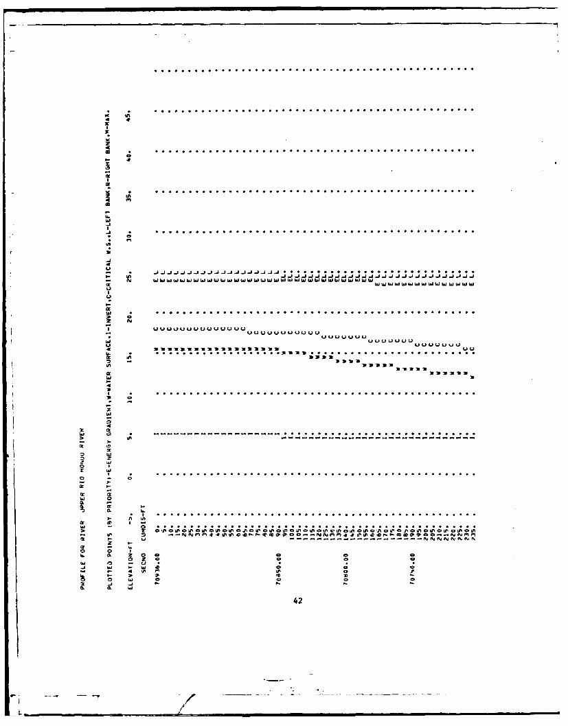
Profile Plot. This plot includes the water surface elevation, the
critical water surface elevation, energy grade line, channel invert,
left and right bank elevations, and the maximum elevation of the cross
section for which hydraulic properties can be computed. The vertical
38

scale of the profile may be determined by the user or by the computer.
Profiles are plotted automatically for jobs using more than five cross
sections, but may be suppressed if desired.
Example
The following pages contain input for a sample profile computation
and normal output, a summary printout and a profile plot.
39
. ./

oUC,o r I
o 'o rUi
0 nZ t 104I I- OD ONN P_0 0 0 n4~~ 0t & I N * M*h i~- -t -0 0 0 .* . * . .tA
Ift*.,z
02IA *0- ! O 0 0 PNN I 4D 0 in n e4A 0 . * 0 0 - . 0 I0 0.0 U0 'a Z0 Io * 0 C! 0. 0 0 1P) t 0 f0 It101
*~~~ C. In V) a wo0*. . 0 * .. 0*o~~~' ODE~ M * NN N tn0
a~ OD N I-.
NN100C0 In- ty z 0t In Nj .. - %u
0. 0 A 00 0 * 0 C2 In In OD0u G21 Do *40
of n - 0 t m300
- I C: N0
C!0C, *0 , cc: *1. - N *c:4,N C N ..* NUs 0 ~ 2 - g .40 0'a
tn -i z 00 fn2 is N5 C:.
c C- .
N ci CN U0 w w 0 N 4 5 4.000 . 0 in c 0 00 0
hi- ~ ~ C u a U 00. IC4 -.V 0 I U ~ .M0 MC' M0 AON 0 > 4 .. - N -N -.26) N U *0
Ix 1. BD 3D.J o *o V .0 a.3r20. u un 2 _j ~ 0o N N ! ; . 4 0.i, fu2 34 -n -
Ct a, 2 I 0 U * O . N Un-2 - N0 0 f n .5 0 * .U *C-o* *)W j C N Z NZ NJ N
tA U0.4 : 0
hi * z In t -O nC -LA 0 3 in a1 z-0 2 I. 0o 0.0 Si CN U .0 0.0~~ N A MA a I @ m UN 0 o h0 *,.tto4
N N M c IV N 4 -A03 u~ tv 0 1N a0
0 40

M p-. p-n p-i I-n* PM N N mN
xl NM 40
04 N p- - 4 00 00 00 00@0 r, m 4 f"@ 00 @ 0
00 ON m N O -WO A 0 0
N NM P40 @0 @oN MA NA N 0 6 I 4 0 @
00~o MN oO: i 4 *
4 M4 r 4 0 m h.
5.. 0i 04 @4-t @0 0" 0
NN NgoN* IS A N 0
VI 0
0~~o 44 Np 4 -M IU .. p 00
j "o .. . . nA 00
* w p-0 MO u- . . .
aNU
UN @0y 0000 03 0 00 0 00 thcc- . . . . .
* hi 0 00 @000u~ ~ . n 0 0 00
A~ ~ 00 @0 00 @0m
"Z 00 M 04 04 ihi - - N4 N-M 3
3 0 00 a- EN 0 Z0uwo m4pp ~ pp
a - -- - t - 4h.NO0 0 mm 00oa00U00 MU0 US0N00
IL 00 00 00 00NJ - iz -
w i 00 00g 00 00 LAO3
0 500
0A 00 p- S -0 N N@
JO .. .. . ; 00 oN gMo~ 07 opWE MM p-N:cc 00 00 . . . .. w
in 00 0 00 0 0 OW0 n00 0
5.5 M-- NE fu N -u( Mr I. 0
m M0.j so go 00 c-0 N--N
a, u . 0 0 0 0 0 0 0 - - - - - -IL 00 00 00NN co 0 00 N
-z S. 0 Z
0b n.5 5. 7
VI J IA0 0 0 0 0 0
K hi 0 0 00 0 00 hi40
-I 1 J ij -b =i --- 1- ijJ iJ- j-
4
I
N I., e deweeooweu) wLoA wwe weWweLa W w eo w ew ww e
-J
....3: a:t ::13:11It3 e:tIIte es. .............. 0......
3 pN
N . . . .. . . . . .. J... J...J.....J..... . J JiJi 5 .J..J
La
Ij
.hi ........... 0 . . . .
0 0
06- LLLLLUi Lii
.... . 2 ....... . ...... .
. .. . ' " .... .2 ... . 'i'i i
44
32 -. . . .. . . . . . ..

Hardware and Software Requirements
HEC-2 has been developed and tested primarily on the UNIVAC 1108
and the Control Data Corporation 6600 computer systems. It has subsequently
been adapted for other machines. The program is written in FORTRAN II and
IV, and includes about 7,000 FORTRAN statements. The following table shows
an approximate comparison of memory requirements and execution speeds
for a number of computers.
HemoryRequirement Speeds
- Computer Words Compile Test
CDC 6600 63,000 59 sec 15 sec
UNIVAC 1108 52,000 b0 sec 50 sec
GE 437 29,000 10 min 5 min
IBM 360/50 70,000 14.5 min 1.7 min(280,000 bytes )
CDC 7600 56,000 8 sec 2 sec
ACKNOWLEDGMENTS
The computer programs described herein have been developed over a
number of years by personnel of The Hydrologic Engineering Center. HEC-l
was developed primarily by Leo R. Beard, recently retired Director of the
HEC. HEC-2 was developed by Bill S. Eichert, Director of the HEC.
43
LIST OF REFERENCES
1. U. S. Army Corps of Engineers, The Hydrologic Engineering Center,"1972 Annual Report," U. S. Army Engineer District, Sacramento, 1972.
2. U. S. Army Corps of Engineers, The Hydrologic Engineering Center,"HEC-1, Flood Hydrograph Package Users Manual," U. S. Army EngineerDistrict, Sacramento, January 1973.
3. U. S. Army Corps of Engineers, The Hydrologic Engineering Center,"HEC-2, Water Surface Profiles Users Manual," U. S. Army EngineerDistrict, Sacramento, February 1972.
44
f-I, - _
l

4
TECHNICAL PAPERS
Technical papers are written by the staff of the HEC, sometimes incollaboration with persons from other organizations, for presentationat various conferences, meetings, seminars and other professionalgatherings. Price
$2.00 each
# I Use of Interrelated Records to Simulate Streamflow, Leo R.Beard, December 1964, 22 pages.
# 2 Optimization Techniques for Hydrologic Engineering, Leo R.Beard, April 1966, 26 pages.
# 3 Methods of Determination of Safe Yield and Compensation Waterfrom Storage Reservoirs, Leo R. Beard, August 1965,21 pages.
# 4 Functional Evaluation of a !,later Resources System, Leo R.Beard, January 1967, 32 pages.
# 5 Streamflow Synthesis for Ungaqed Rivers, Leo R. Beard,October 1967, 27 pages.
# 6 Simulation of Daily Streamflow, Leo R. Beard, April 1968,19 oaqes.
# 7 Pilot Study for Storage Requirements for Low Flow Augmenta-tion, A. J. Fredrich, Anril 1968, 30 pages.
# 8 Worth of Streamflow Data for Project Design - A Pilot Study,D. R. Dawdv, H. E. Kubik, L. R. Beard, and E. R. Close,April 1968, 20 pages.
# 9 Economic Evaluation of Reservoir System Accomplishments,Leo R. Beard, May 1968, 22 pages.
#10 Hydrologic Simulation in Vater-Yield Analysis, Leo R.Beard, 1964, 22 pages.
#11 Survey of Programs for Water Surface Profiles, Bill S.Eichert, August 1968, 39 pages.
#12 Hypothetical Flood Computation for a Stream System, LeoR. Beard, April 1968, 26 paqes.

TECHNICAL PAPERS (Continued) Price$2.00 each
#13 Maximum Utilization of Scarce Data in Hydrologic Design,Leo R. Beard and A. J. Fredrich, March 1969, 20 pages.
#14 Techniques for Evaluating Long-Term Reservoir Yields,A. J. Fredrich, February 1969, 36 pages.
#15 Hydrostatistics - Principles of Application, Leo R. Beard,July 1969, 18 pages.
#16 A Hydrologic Water Resource System Modelinq Techniques,L. G. Hulman and D. K. Erickson, 1969, 42 pages.
#17 Hydrologic Engineering Techniques for Regional WaterResources Planning, Augustine J. Fredrich and Edward F.Hawkins, October 1969, 30 pages.
#18 Estimating Monthly Streamflows Within a Region, Leo R.Beard, Augustine J. Fredrich, Edward F. Hawkins, January1970, 23 pages.
#19 Suspended Sediment Discharge in Streams, Charles E. Abraham,April 1969, 24 pages.
#20 Computer Determination of Flow Through Bridges, Bill S.Eichert and John Peters, July 1970, 32 pages.
#21 An Approach to Reservoir Temperature Analysis, L. R. Beardand R. G. Willey, April 1970, 31 pages.
#22 A Finite Difference Method for Analyzing Liquid Flow inVariably Saturated Porous Media, Richard L. Cooley,April 1970, 46 pages.
#23 Uses of Simulation in River Basin Planning, William K.Johnson and E. T. McGee, August 1970, 30 pages.
#24 Hydroelectric Power Analysis in Reservoir Systems, AugustineJ. Fredrich, August 1970, 19 pages.
#25 Status of Water Resource Systems Analysis, Leo R. Beard,January 1971, 14 pages.
#26 System Relationships for Panama Canal Water Supplv,Lewis G. Hulman, April 1971, 18 oaqq.This pubZication is not available to countries outside ofthe U.S.
T
TECHNICAL PAPERS (Continued) Price$2.00 each
#27 Systems Analysis of the Panama Canal Water Supply, David C.Lewis and Leo R. Beard, April 1971, 14 pages.This publication is not available to countries outside ofthe U.S.
#28 Digital Simulation of an Existing Water Resources System,Augustine J. Fredrich, October 1971, 32 pages.
#29 Computer Applications in Continuing Education, Augustine J.Fredrich, Bill S. Eichert, and Darryl W. Davis, January1972, 24 pages.
#30 Drought Severity and Water Supply Dependability, Leo R. Beard.and Harold E. Kubik, January 1972, 22 pages.
#31 Development of System Operation Rules for an Existing Systemby Simulation, C. Pat Davis and Augustine J. Fredrich,August 1971, 21 pages.
#32 Alternative Aporoaches to Water Resource System Simulation,Leo R. Beard, Arden Weiss, and T. Al Austin, May 1972,13 pages.
#33 System Simulation for Integrated Use of Hydroelectric andThermal Power Generation, Augustine J. Fredrich and Leo R.Beard, October 1972, 23 pages.
#34 Optimizing Flood Control Allocation for a MultipurposeReservoir, Fred K. Duren and Leo R. Beard, August 1972,17 pages.
#35 Computer Models for Rainfall-Runoff and River HydraulicAnalysis, Darryl W. Davis, March 1973, 50 pages.
#36 Evaluation of Drought Effects at Lake Atitlan, Arlen D. Feldman,September 1972, 17 pages.This publication is not available to countries outside ofthe U.S.
#37 Downstream Effects of the Levee Overtopping at Wilkes-Barre,PA, During Tropical Storm Agnes, Arlen D. Feldman, April1973, 24 pages.
#38 Water Quality Evaluation of Aquatic Systems, R. G. Willey,April 1975, 26 pages.
#39 A Method for Analyzing Effects of Dam Failures in DesignStudies, William A. Thomas, August 1972, 31 pages.
1~?

T
TECHNICAL PAPERS (Continued) Price$2.00 each
#40 Storm Drainage and Urban Region Flood Control Planning,Darryl Davis, October 1974, 44 pages.
#41 HEC-5C, A Simulation Model for System Formulation andEvaluation, Bill S. Eichert, March 1974, 31 pages.
#42 Optimal Sizing of Urban Flood Control Systems, DarrylDavis, March 1974, 22 pages.
#43 Hydrologic and Economic Simulation of Flood Control Aspectsof Water Resources Systems, Bill S. Eichert, August1975, 13 pages.
#44 Sizing Flood Control Reservoir Systems by Systems Analysis,Bill S. Eichert and Darryl Davis, March 1976, 38 pages.
#45 Techniques for Real-Time Operation of Flood Control Reservoirsin the Merrimack River Basin, Bill S. Eichert, John C.Peters and Arthur F. Pabst, November 1975, 48 pages.
#46 Spatial Data Analysis of Nonstructural Measures, Robert P.Webb and Michael W. Burnham, August 1976, 24 pages.
#47 Comprehensive Flood Plain Studies Usinq Spatial Data Manage-ment Techniques, Darryl W. Davis, October 1976, 23 pages.
#48 Direct Runoff Hydroqraph Parameters Versus Urbanization,David L. Gundlach, September 1976, 10 pages.
#49 Experience of HEC in Disseminating Information on HydrologicalModels, Bill S. Eichert, June 1977, 12 pages.(Superseded by TP#56)
#50 Effects of Dam Removal: An Approach to Sedimentation,David T. Williams, October 1977, 39 pages.
#51 Design of Flood Control Improvements by Systems Analysis:A Case Study, Howard 0. Reese, Arnold V. Robbins, JohnR. Jordan, and Harold V. Doyal, October 1971, 27 pages.
#52 Potential Use of Digital Computer Ground Water Models,David L. Gundlach, April 1978, 40 pages.
#53 Development of Generalized Free Surface Flow Models UsingFinite Element Techniques, D. Michael Gee and Robert C.MacArthur, July 1978, 23 pages.
#54 Adjustment of Peak Discharge Rates for Urbanization,David L. Gundlach, September 1978, 11 pages.
___ .... :I I zI I,...- I~ I

Price
TECHNICAL PAPERS (Continued) $2.00 each
#55 The Development and Servicing of Spatial Data ManagementTechnioues in the Corps of Engineers, R. Pat Webb andDarryl W. Davis, July 1978, 30 pages.
#56 Experiences of the Hydrologic Engineering Center in Main-taining Widely Used Hydrologic and Water Resource ComputerModels, Bill S. Eichert, November 1978, 19 pages.
#57 Flood Damaqe Assessments Using Spatial Data ManaqementTechniques, Darryl W. Davis and R. Pat Webb, May 1978,30 pages.
#58 A Model for Evaluating Runoff-Ouality in MetropolitanMaster Planning, L. A. Roesner, H. M. Nichandros,R. P. Shubinski, A. D. Feldman, J. 1-. Abbott, and A. 0.Friedland, April 1972, 85 nages.
#59 Testing of Several Runoff Models on an Urban Watershed,Jess Abbott, October 1978, 56 pages.
#60 Operational Simulation of a Reservoir System with PumpedStorage, George F. McMahon, Vern Bonner and Bill S.Eichert, February 1979, 35 pages.
#61 Technical Factors in Small Hydropower Planning, Darryl W.Davis, February 1979, 38 pages.
#62 Flood Hydrograph and Peak Flow Frequency Analysis, Arlen D.Feldman, March 1979, 25 paqes.
#63 HEC Contribution to Reservoir System Operation, Bill S.Eichert and Vernon R. Bonner, August 1979, 32 pages.
#64 Determining Peak-Discharge Frequencies in an UrbanizingWatershed: A Case Study, Steven F. Daly and John Peters,July 1979, 19 pages.
#65 Feasibility Analysis in Small Hvdropower Plannina, Darryl14. Davis and Brian Y. Smith, Aunust I7l, 24 panes.
#66 Reservoir Storage Determination by Computer Simulation ofFlood Control and Conservation Systems, Bill S. Eichert,October 1979, 14 panes.
'467 Hydroloric Land Use Classification Usinq LANDSAT, Robert ,J.Cermak, Arlen D. Feldman, and R. Pat Webb, October 1979,30 pages.
-L~
TECHNICAL PAPERS (Continued) Price
$2.00 each
#68 Interactive Nonstructural Flood-Control Planning, David T.Ford, June 1980, 18 pages.
#69 Critical Water Surface by Minimum Specific Energy Using theParabolic Method, Bill S. Eichert, 1969, 14 pages.
#70 Corps of Engineers' Experience with Automatic Calibrationof a Precipitation-Runoff Model, David T. Ford,Edward C. Morris, and Arlen D. Feldman, May 1980,18 pages.
#71 Determination of Land Use from Satellite Imagery for Inputto Hydrologic Models, R. Pat Webb, Robert Cermak, andArlen Feldman, April 1980, 24 pages.
#72 Application of the Finite Element Method to Vertically StratifiedHydrodynamic Flow and Water Ouality, Robert C. MacArthurand William R. Norton, May 1980, 12 pages.
#73 Flood Mitigation Planning Usinq HEC-SAM, Darryl W. Davis, June1980, 23 pages.
#74 Hydrographs by Single Linear Reservoir Model, John T. Pederson,John C. Peters, Otto J. Helweg, May 1980, 17 pages.
#75 HEC Activities in Reservoir Analysis, Vern R. Bonner,June 1980, 16 paqes.
44

DATFILMEI
I )I