MPRAMunich Personal RePEc Archive

Endogenous Firm and Information RentUnder Demand Uncertainty

Yanfei Li and Shuntian Yao and Wai-Mun Chia

Nanyang Technological University, Nanyang TechnologicalUniversity, Nanyang Technological University

12. February 2009

Online at http://mpra.ub.uni-muenchen.de/14867/MPRA Paper No. 14867, posted 1. May 2009 05:00 UTC

1

Endogenous Firm and Information Rent under Demand Uncertainty

Yanfei Li *, Shuntian Yao**, and Wai-Mun Chia***

Authors’ affiliation: Division of Economics, School of Humanities and Social Sciences, Nanyang Technological University

Nanyang Avenue, Singapore, 639798

April 2009

Abstract: Increasing evidence shows that ICT (Information and Communication Technology) investment

improves firm performance. This paper takes the firm as information processing unit, putting it in

stochastic environment. It provides a model that involves the division of labor and specialization,

and demand uncertainty. It shows that conditionally, a firm with information processing ability

comes into being endogenously, with information rent generated. The size of the rent depends on

the level of uncertainty, market competition, and the firm’s information processing ability. Finally,

case studies on the financial industry and the wholesale and retail industry of 10 OECD countries are

conducted.

Keywords: demand uncertainty, information processing, firm, information rent

JEL classification: D2; D4; D8; L1; L2

* Correspondence author. Email address: h060012@ntu.edu.sg, Tel: +65-91813089.

**Email: ASTYAO@NTU.EDU.SG

***Email: ASWMCHIA@NTU.EDU.SG

Acknowledgement: We are grateful to Prof. Dennis Carlton, Dr. John Lane, Mr. Alfredo Burlando, and Ms. Qiyan Ong for their helpful comments. All remaining errors are ours.

2

I. Introduction

The relation between firm and information needs to be clarified for both practical and theoretical

reasons. On the practical side, many questions have been raised regarding the impact of ICT

(Information and Communication Technology) on economic growth. Gradually the focus of interest

has moved from nation level to firm level. Jorgenson and Stiroh (2000), Oliner and Sichel (2000), and

Jorgenson (2001) generally confirm that ICT contributed around 1/3 of the economic growth in the

U.S., through capital-deepening effect and TFP acceleration. Industrial level studies by Stiroh (2002),

van Ark et al. (2002), Oulton and Srinivasan (2005) show that the service industries benefited most

from investment in ICT, and that other OECD countries lagged behind the U.S. in exploiting the

advantages brought by ICT. An EU commission report by Barrios and Burgelman (2007) indicates a

“first-mover advantage” of the U.S. in applying ICT. This is not surprising since Apte and Nath (2004)

reported that by 1997, 63% of the U.S. GNP is consisted of “information economy”, which is

information-related economic activities; and the service industries generally saw a growth in

information-related activities.

Furthermore, Bryjolfsson and Hitt (2000) provide firm-level evidence that ICT contributes to firm

productivity and that organizational investment as a complementary investment to ICT investment is

important. Matteucci et al. (2005) find firm level evidence that, in the second half of 1990s,

European OECD countries benefited from their ICT investment, with manufacturing sector benefited

more than service sector, yet generally are lagged behind as compared to the U.S. performance.

Accordingly, we ask what do firms do with information, and how information technology affects

firms’ performance.

On the theoretical side, information economics has shown us that information plays essential role in

explaining issues in contract design at individual level and firm level (Macho-Stadler et al. 2001),

such as insurance policy, signaling, screening, share-cropping, and corporate governance. Beyond

that, information is also important in explaining equilibriums of the overall economy, for example,

the role of information in wage policy (labor market equilibrium), in equity market (allocation of

financial resources), in diversification of prices, and in money market stability (Stiglitz, 2002).

Moreover, other economic theories of information have been developed over time. Marschak (1954)

and Arrow (1971, 1985) discuss the economic value of information. The Arrow (1971, 1985) papers

manage to link economic value of information to the Shannon measure of information. Weitzman

(1974) discuss the efficiency of two different institutions when uncertainty exists in a system, which

3

assumes imperfect information. Radner and Stiglitz (1984) show that there is nonconcavity in the

value of information: Having little information is worse than having no information at all.

Given the importance of information in economic analysis, it also enters the theories of firm.

Marschak (1954) introduces firm’s structure with corresponding information processing procedure

to analyze the value of information. Aoki (1986) distinguishes two alternative organizational

structures of a firm: horizontal vs. vertical. And he found the conditions under which one is more

efficient than the other when production uncertainty is embedded in the system. With organization

costs under different firm structures considered, Carter (1995) discusses the effectiveness of seven

different firm structures in processing information to reduce uncertainty, and thus to improve firm

performance. Arrow (1975) points out that in an industry with upstream firms and downstream

firms, downstream firms tend to vertically integrate to acquire input information to reduce

uncertainty in input supply. And the industrial market tends to evolve from being competitive to

imperfect competition as vertical integration provides market power. DeCanio and Watkins (1998)

interpret and model the firm as an information processing network. Within this framework, the

effect of different organizational structure on efficiency of the firm is discussed. Marschak (2004)

provided a discussion on how IT investment, which is supposed to lower down information gathering

cost, help a firm shift to a decentralized organizational form.

The above mentioned literature implies to us that there must be some connection among

information processing, organizational structure, ICT investment, and firm performance. Yet the

picture is not really clear or comprehensive.

While efforts have been made to provide explanations linking information processing, organizational

structure, ICT investment and firm’s performance in one way or another, no comprehensive model

has yet been developed to link them together. Therefore, in an attempt to accomplish this specifc

aim, we see the firm as an information processing unit, which emerges endogenously from industrial

markets with demand uncertainties. Information processing ability, which varies from firm to firm, is

seen as the only thing that distinguishes firm production from non-firm production. ICT investment,

in this model, is assumed to reduce the cost of information processing. We show that the unique

informational advantage brings firm a surplus which is reasonably argued as information rent,

conditional on a few key parameters, including the level of uncertainty, the degree of market

competition, and the cost of information processing1.

1 If one carries this point of view further, with matured financial market, the return to any productive factor, say labor skill, management, capital goods, can be capitalized in its market price. Thus any productive factor is readily available from market. Yet after compensating all factors employed, modern firms still stand to acquire

4

We also apply the framework of our theory to the data of the wholesale and retail industry and the

financial intermediation industry from 10 OECD countries. We investigate the mechanism and the

extent that the aggregate firm performance – measured as multi-factor productivity – of the

industry is decided by ICT investment, intensity of market competition, as well as average firm size. It

is found that the two industries actually have different market structures, from which we infer

different patterns of impact from the above factors. Interestingly, we do not observe any “first-

mover advantage”. Our results suggest that industries in different countries could choose their

specific optimal level of ICT investment according to their own market structure – not necessarily the

higher the better.

The rest of the paper is organized as follows. Section 2 provides the very theoretical backgrounds

which lay out the building blocks of our model. Section 3 gives detailed descriptions of the model.

Section 4 discusses the main findings of the model. Section 5 discusses the implications derived from

the model. Section 6 is devoted to case studies into the financial industry and the retail industry.

Section 7 concludes.

II. Theoretical Issues

This section lays out the building blocks of the model. First piece is about endogenous firm and

information.

Malmgren (1961) was among the first to ask why multi-person, multi-process firms exist in a

competitive economy. In his view, a firm functions as an allocating mechanism of inputs and outputs.

economic surplus – expected sustainable profit. In this sense, all unique advantages that a firm holds to generate this profit, be it technological or organizational, can be replicated by obtaining equivalent inputs such as manpower, human capital, or licenses from competitive markets of factors. The only thing that hinders one firm from replicating another is its information processing ability, namely the ability to acquire the best inputs and to process the information of the inputs in order to put them into the right positions.

Additionally, as information processing is a costly activity, efforts devoted to reduce such cost which include IT investment and its complementary organizational investment are supposed to positively affect performance of the firm.

5

The reason why such allocation is not done by markets, which is supposed to be efficient within

traditional settings, is because of the uncertainty and incomplete information2 that embed in real

economy. Even if we talk about expectational equilibrium3, static general equilibrium in this case is

difficult to be reached, due to the formidable amount of information to coordinate individual

producers. Therefore, firstly firms arise to reduce the information requirement by integrating

production procedures, vertically and horizontally, making the convergence of expectations possible.

Secondly, firms arise to process internal and external information, which in return gives firms higher

expected profit.

Malmgren (1961) also discussed the two types of information processed by a firm: internal

information regarding the production-related variables; and external information regarding the

environment4 – the intermediate input market and the product market. Casson (1997) further

developed the idea as that firms’ internal structure would routinize the processing of external

information to be the processing of internal information, leaving the remaining external information

to the entrepreneurs. For the purpose of this paper, we focus on the routine information processing

conducted by established firm structure.

The second piece is about convex production technology. Yang and Ng (1995) provided a general

equilibrium framework in which firms are endogenously derived out of economic incentive. For their

purpose, convex production technology was assumed with multi-stage production. Their argument

was that firms substitute market in coordinating production procedure where transaction cost is too

high. It is worth of pointing out that they assumed an environment with certainty, and the issues of

information and coordination are not included.

The third piece is about demand uncertainty and availability. Carlton (1978) introduced a simple

one-product economy with both demand and supply uncertainties. The existence of firms is given

exogenously. The product is featured in the market by both its price and availability (possibility of

obtaining the product from a supplier given a certain price). In this economy, it is possible that each

firm makes a different decision on its production and pricing. It is shown that, however, with each

party trying to maximize its expected profit or utility, given identical production technology and

2 Incomplete information here refers to not knowing what everyone else knows (Malmgren, 1961). This is distinguished from the concept of imperfect information, which means not knowing what everyone else has done. 3 Individual agents in the economy can still maximize their expected utility or profit. Arrow (1964) and Debreu (1959) have shown that when agents are coordinated by a Walrasian auctioneer, market is cleared with a certain set of prices. In this way, equilibrium can be achieved. However, in Malmgren’s case, by assuming away the Walrasian auctioneer, the economy cannot automatically find and converge to an expectational equilibrium. 4 Malmgren (1961) refers to external information as dependent on the so-called “structure of market”.

6

utility function, the economy converges to one combination of price and availability. When demand

uncertainty decreases, the economy moves closer to equilibrium under certainty, which means a

uniform price equal to marginal cost and one hundred percent availability. Carlton and Dana (2008)

further extended the framework to multi-industries with quality issue considered.

The forth piece is about intermediate input and vertical integration. As an extension of Carlton

(1978), Carlton (1979) took the existence of firms as given, and assumed that initially firms distribute

in both the upper stream and the lower stream of a multi-stage production procedure. Uncertainty

in demand and input supply was assumed. It was shown that firms could have better performance

by vertically integrating both the production of the lower and higher stream. Vertical integration

could be seen as the the integrated firm acquiring information from the complementary stage of

production.

Based on the above mentioned blocks of knowledg, namely information economics, firm theory, and

general equilibrium under uncertainty, a model of endogenous firms in a market under demand

uncertainty would be developed. The firm, with it’s ability of information processing, would be

rewarded information rent as its sustainable source of profit.

III. The Model

III(i). Model Settings

In a specific industry, it is assumed that there are only one intermediate input M and one final

product X . Each individual agent engaged in the industry is endowed with L labor time which we

normalize it to one, and is capable of producing either of them using the following technologies:

(1 )

aM

aX

m l

x m lα α−

=

= ⋅,

where 1a > , 0 1α< < .

Xl and Ml denote the portions of L devoted into production of X and M , respectively. The

production technology does not allow two individuals to work together additively or multiplicatively

in one production procedure, which means for each individual 1Xl ≤ , 1Ml ≤ , and 1X Ml l+ = .

7

Assume that the markets for both M and X exist. With the convex production technologies above,

individuals as producers prefer specialization in producing one product only and then trade in the

market, given identified expected profitable price and demand.

Production in the overall industry could then be coordinated via intermediate input market for M .

Namely, a portion of the population MR in the industry specializes in producing M , while the other

portion of the population XR in the industry specializes in producing X . The latter purchases M

from the former in order to produce X , and sell their products in the final product market for X .

Each of them runs his own shop, with only himself employed, to sell their products. This system is

thereafter referred to as a ‘market-organized production’ with full specialization of each individual.

However, due to imperfect information5 with both buyers and producers, for both markets, no buyer

knows how many others would go to the same shop as he does; and no producer knows how many

buyers would drop by. It leads to availability problem when there are too many buyers and the shop

runs out of stock. Therefore the availability can be taken as the probability of the event that the

shop runs out of stock.

Now, what the buyer knows is the price and availability (a kind of quality) that a shop offers; and

what the producers know is that they face random demand, which in this model we assume it to be

subject to a uniform distribution with parameter λ . The availability of the final product is decided

by the output level of the shop6 , which is common knowledge to both the buyers and the producers.

Thereby we have assumed complete information for buyers here, for simplicity. This imperfect

information setting allows the possibility that individual shops ask for arbitrary price given his

availability, because demand is given exogenously and therefore perfect competition is no longer

the case .

However, complete information for buyers means competition still exists among shops, regarding

the policies of price and availability combinations. And such applies to both the intermediate input

5 This is due to the setting of our model that consumers decide simultaneously which shop to visit. For each consumer, he/she doesn’t know what the others have decided. Thus it is imperfect information, rather than incomplete information. 6 This assumption was used by Carlton (1978). The availability issue is incurred by uncertain demand. When realized demand exceeds suppliers’ production level, which is decided according to their expectation, availability is no longer one hundred percent. For such a setting, there are two implicit assumptions. Firstly, production plan is implemented before the demand is realized. Secondly, each consumer enquires with any shop for only once. If the shop runs out of stock, the consumer won’t be able to try another shop. For simplicity of our analysis, the current paper modifies the second assumption into that for each unit of demand, buyer tries only one shop.

8

market and the final product market. It is shown later that there exists a unique equilibrium, in

which prices of the products convey information on the intensity of market competition.

As consumers, individuals consume X . With availability considered, the utility of consuming x units of X is:

( , )X Xc A c AU f x Q x Q≡ = ⋅ .

XAQ is the availability of the commodity, which is measured as the probability of obtaining X 7. The

availability of the commodity can be taken as a kind of quality of it.

III(ii). Consumer Behavior

A typical consumer’s decision problem is,

max.

. . ( )

XA

XX A

U x Q

s t P Q x I

= ⋅

⋅ =,

where I is the exogenous income8.

XP is the price of X . Intuitively, the price one pays for the X product is a function of the

availability (quality) that one is looking for. It is also intuitive that 0XXA

PQ∂

>∂

9. To maximize utility,

consumers would require the combination of price and availability offered by a shop to satisfy the

first order condition10:

7 And it will be illustrated in the subsection for the X -producers’ behavior. 8 Note that this is not a closed one-industry economy. Rather, the object under study is one specific industry from a multi-industry economy. Consumers come to consume this industry’s product with their income each earned from this industry or from other industries. For this reason, income constraint is not an endogenous variable. And thus the utility function is specifically for the consumption of products of this specific industry. 9 Availability can be seen as quality of the product. For this reason, the X - producer does not necessarily consume his own product, as he may well produce and sell high quality product, but consume low quality product, according to his preference. Thus what he cares about, as the m producers do as well, is the monetary revenue he receives from the market.

10 Put Lagrange function as ( ( ) )X XA X Ax Q I P Q xψ ν= ⋅ + ⋅ − ⋅ . F.O.C. gives ( ) 0X X

A X AQ P Qxψ

ν∂

= − ⋅ =∂

and '( ) 0XX AX

A

x x P QQψ ν∂

= − ⋅ ⋅ =∂

. Thus '( ) 1( )

XX A

X XX A A

P QP Q Q

= . Treating it as a differential equation with

9

0

( )X

X AX A

QP Q

β= . (2.1)

Parameter 0β is the reverse of the shadow price of obtaining one unit of X with certainty (not the

one unit of demand realized with availability smaller than 1). It is decided by product market

competition at the equilibrium, as will be seen later.

Since 0X

X A

IIx

P Qβ⋅

= = , it can be shown that 0XA

xQ∂

<∂

, as well as that 2

2 0( )X

A

xQ∂

>∂

.

Actually, when pricing condition 0β has been decided, maximum utility is fixed at *0U I β= ⋅ .11

Thus we have the following diagram:

(Place Figure 1 approximately here)

Figure 1: Indifference curve of utility function and the budget constraint of consumer

It can be observed that the indifference curve of maximum utility overlaps with the budget

constraint curve. And the position of the ( , )xAQ x curve depends on ��. The optimal combination of

xAQ and x for the consumers could be any point along the *U curve.

III(iii). The Individual X -Producers’ Decision

On the demand side, an individual X -producer faces random demand with a uniform distribution,

which could be described by parameter 1λ . The probability density of the uniform distribution for

the X -producer is 1

1

1( )kλφ λ

= , 1[0, ]k λ∈ , where k denotes the realization of per shop random

demand. It can be inferred that the larger the parameter 1λ , the greater the volatility in terms of

variance in the market.

unknown function ( )XP ⋅ , it can be written as ln ( ) 1X

X AX XA A

d P QdQ Q

= . By integration,

ln ( ) lnX XX A AP Q Q c= + , and ( )X c X

X A AP Q e Q= ⋅ . Let 0ceβ = , we get equation (2.1).

11 Note that although this result shows that consumers choice on price and quality combination has no effect on utility gained, the optimization is necessary and important in the sense that it imposes constraint on producer’s pricing behaviour, as will be shown later.

10

On the production side, the X -producer buys Xm units of the intermediate input. And then with

full specialization, his output level is (1 )aXm Lα α⋅ −⋅ . With L normalized to one, the output level of

each X -producer simply is Xmα . Next, the X -producer needs to decide how many units of � to

purchase from the market by maximizing his expected revenue.

Charging a price of iXP , the revenue function of the i th X -producer is:

, if ={

, if iX

iX

P k k m

m P k m

α

α απ

≤

>.

To maximize his expected revenue, the i th X -producer would decide the optimal output and price

levels according to:

1 1

0

*

max. ( ) ( ) ( ) ( )

s.t. ( )

X

A

X

iX A

mM

X iX X iX M X M

m

XP iX

iX

E P k k dk m P k dk P m Q P

IU Q P U

P

α

α

αλ λπ φ φ

∞ = + −

= ≥

∫ ∫,

where ( )A

MMQ P is the availability of intermediate input M from the intermediate input market.

The constraint condition is a reinterpretation of eq. (2.1), and means that the X -producer needs to

offer a combination of price and availability that delivers a utility at least as high as the average level

in the market.

The constraint condition is equivalent to the consumers’ optimization condition – eq. (2.1). *U is

the average level of utility which a typical consumer can obtain from the market, by consuming with

a certain combination of XP and ( )A

XXQ P . A seller thus has to provide a combination of price and

availability which makes consumers at least as well off as this one.

Given his output level, this constraint condition actually decides the price that the X -producer can

charge: Since 1( ) ( )

A

X MA X MQ F k m Q Pα

λ= < × is the availability (1 1

0

( ) ( )Xm

XF k m k dkα

αλ λφ< = ∫ , the

cumulative density function), the i th X -producer can charge a price

1

0

( ) ( )A

MX M

iX

F k m Q PP

αλ

β< ×

= , according to eq. (2.1).

11

Given iXP as exogenous, the X -producer is to decide the price and the quantity to purchase

intermediate input M , as there possibly exists muliple combinations of price and availability of M

to choose. Similar with the case of final product �, the availability of � is a function of the price that

the buyer – X -producer – is willing to accept.

It’s not difficult to show according to F.O.C. of the X -producer’s maximization that12 :

1A

MMQ Pβ= . (2.2)

1β is subject to equilibrium of the competitive market of intermediate input M .

And the demand for � is decided by the F.O.C.:

2 11

1

X MX

iX

m Pm

P

αα α

αλ

−− − = . (2.3)

Accordingly, expected revenue of the � - producer is:

1

1 1

0 10

( ) ( ) ( )( ) ( ) ( ) ( )

X

A A

A

X

M MmX M M M

X X X M

m

F k m Q P Q PE k k dk m k dk m Q P

α

α

αλ α

λ λπ φ φβ β

∞ < × = + − ⋅

∫ ∫ .

III(iv). The M - Producers’ Decision

Again let � denote the realized per shop random demand on M . A typical M - producer faces

random demand which is subject to uniform distribution parameterized by 2λ , such that

12 iXP is exogenous to the X -producer’s optimization problem at this moment for two reasons: on the one

hand the producer can decide arbitrarily to charge any price he wants and it is only when the market converges to the equilibrium that he is bounded by the constraint condition; on the other hand the price is to

be determined by 0β in the equilibrium, which is an exogenous variable to individual producers.

Thus we have 1 1

0

( )' ( ( ) ( ) ) 0

X

X

mM MA iX X M X A X

M m

EQ P kP k dk m P k dk P m Q m

P

α

α

αλ λ

π ∞ ∂= ⋅ ⋅ + − ⋅ − ⋅ =

∂ ∫ ∫ , and

1 1

0

( )( ) ( ) ( ) '( ) 0

X

X

mM M M

iX X iX M A X A M A XMA m

EP kP k dk m P P k dk P Q m Q P Q m

Q

α

α

αλ λ

π ∞ ∂= + − − ⋅ ⋅ =

∂ ∫ ∫ .

Combining the two we have 1

'' MM

A

PQ

= , which gives us equation (2.2).

12

2

2

1( )kλφ λ

= is the probability density function, 2[0, ]k λ∈ . Parameter 2λ describes the volatility in

the intermediate input market, and is itself partially decided by the professional distribution of

population: x

m

RR

13. However, there is a precondition for the M - producer to fully specialize in the

production of �: 2 1λ ≥ . Otherwise, given that an � - producer knows that the maximum of

demand coming to him is less than one, there is no reason to fully specialize in the production of M :

1 1a = .

The revenue function for the i th M - producer is,

, if 1={

, if 1iM

iM

P k kP k

π≤>

.

The M -producer faces a decision problem of:

2 2

1

0 1

*

max. ( ) ( ) ( )

s.t. ( | ) ( )

iM iM

X iM X

E P k k dk P k dk

E P E

λ λπ φ φ

π π

∞

= +

≥

∫ ∫.

The constraint condition is equivalent to the X -producers’ optimization condition – eq.(2.2). It

means that the combination of price and availability of � offered by one � - producer in the market

should provide the buyer – X -producers – with an expected revenue at least as high as the average

level. Given that the � - producer’s output level is fixed at 1 (if 2 1λ ≥ ), the constraint condition

already decides the price that can be charged for �at the equilibrium: 2

1

( 1)iM

F kP λ

β<

= , since

2 2

1

0

( ) ( 1) ( )A

MiMQ P F k k dkλ λφ= < = ∫ .

Accordingly, expected revenue of the M -producer is14:

13 Intuitively, 2λ (as well as 1λ ) describes the largest possible demand that one shop-runner might face. It

must be jointly decided by factors like the size of the population of buyers and purchasing power of the buyers.

14 With uniform distribution, 2

1 2

11

( ) (1 )2ME

λπβ λ

= ⋅ −⋅

. Thus ( )ME π increases as 2λ decreases.

13

2

2 2

1

1 0 1

( 1)( ) ( ) ( )m

F kE k k dk k dkλ

λ λπ φ φβ

∞< = +

∫ ∫ .

The only decision for the �-producer at the equilibrium is whether he wants to stay in the industry.

When his expected revenue deteriorates, he might wish to leave. With the exit of some M -

producers, parameter 2λ would adjust to push up the expected revenue of the rest of the M -

producers.

III(v). The Equilibrium of Market-Organized Production

That individually specialized X and M producers implement the two-stage production procedure

via market transactions of intermediate input M is referred to as market-organized production.

Since we have identical consumers and producers in this economy, it is intuitive that the equilibrium

of this economy is a certain combination of price and availability for each of the two products, to

which all producers and buyers would converge.

Proposition 1: The equilibrium in which the producers in either market produce at the same output

level to offer the same availability and sell their product at the same price is stable.

Take the X -producer as an example. Given such equilibrium has been achieved, suppose that firm

i disobeys the equilibrium ( , )A

XXP Q and raises its price, resulting in no purchase from the

consumers because of its higher price with the same availability as before. However, it is possible

that he uses the higher price to pay for the higher production cost to increase availability of his

products. To do this, note that the availability of intermediate input is virtually fixed because the M

-producer cannot increase its production anymore, so the X -producer cannot get higher availability

of M , by paying a higher price. The only way to increase output, and thus availability, is to increase

its purchase of M . Nevertheless this is not revenue maximizing, as the marginal product of �

would decrease, which means that the cost incurred by increasing production is to be higher than

the possible increase in the price of X .

Alternatively, if one deviates by quoting a price lower than xP , he loses expected profit if he

produces at equilibrium output level. However, if he chooses to cut down his output level, the

marginal product of M would be higher than the price of � in the market, which implies that he

should increase his production.

14

Thus we find that the equilibrium is stable at least in its neighbourhood. A formal proof of this point

can be found in the appendix A.

The other important property of the equilibrium is:

( ) ( )X ME Eπ π= . (2.4)

This property helps us determine the pricing parameters 0β and 1β . Without loss of generality, the

price of M is normalized as 1MP = . Then we have:

2

212

( 1) 1( 1)

2M

F kF k

Pλ

λβλ

<= = < = .

Using eq. (2.4), we have 0β in terms of Xm - the optimal quantity of M that X - producers would

like to purchase.

2 1 1 1

2 2 2

2

0

0 1

0 1

( 1) ( ) ( ) ( )

( ) ( ) ( 1)

X

x

m

X X

m

X

F k F k m k k dk m k dk

k k dk k dk m k

α

α

α αλ λ λ λ

λ λ λ

φ φ

βφ φ φ

∞

∞

< ⋅ < +

=+ + ⋅ <

∫ ∫

∫ ∫

Applying the above results to equation (2.3), when 12

α = , Xm can be solved in terms of 1λ and 2λ .

Thus, the output level of the X - producer is 12

Xq m= , which assumes different value according to

the specific values of 1λ and 2λ (Figure 2)15.

(Place Figure 2 approximately here)

Figure 2: Output level q of x -producers with specific values of 1λ and 2λ .

Since 0β can be written in terms of Xm , 0β is also determined by 1λ and 2λ (Figure 3).

15 For certain combinations of ( 1λ , 2λ ), Xm turns negative, simply because specializing in producing X is no

longer optimal, due to volatile uncertainty in the markets. Mathematically, we could add non-negative constraint to the X - producer’s maximization problem, which gives us corner solutions and eliminate the negative part. However, doing this would not influence any of our major conclusions.

15

(Place Figure 3 approximately here)

Figure 3: Pricing parameter 0β with specific values of 1λ and 2λ .

It is not difficult to observe that both output level and pricing parameter assume values with

economic sense within certain range of ( 1λ , 2λ ).

III(vi). Firm Production

Now we derive firms with features identified by Malmgren (1961): a multi-person, multi-process

mechanism of allocating inputs and outputs. To examine our hypothesis, the firm derived in this

model is assumed with no advantages in terms of production technology or retail channels (Figure 4).

(Place Figure 4 approximately here)

Figure 4: The structure of a firm

As illustrated by Figure 4, a firm hires individuals from the labor market, making them specialize in

the production of either � or X . The production and supply of M is pooled together, and then

distributed to individual X –shops of the firm. The production and supply of X is still done at

individual shops. We also assume that the shops are relatively independent and do not

communicate with each other. Thus the only difference between the firm production and the

market-organized production is that a labor market replaces the intermediate input market. By

doing this, a firm processes the information of supply and demand of the intermediate input within

the firm.

At each X -shop, the expected revenue is:

1 1

0

( ) ( )f

f

m

X f

m

P k k dk m k dk

α

α

αλ λφ φ

∞ + ∫ ∫ .

Decision problem for the firm to maximize its expected profit is, when there are i shops:

1 1

0

max. ( ) ( ) ( ) ( 1) ( ( 1))f

f

m

f X i i i f i i f fi m

E P k k dk m k dk w i m C i m

α

α

αλ λπ φ φ

∞ = + − × × + − ⋅ +

∑ ∫ ∫

16

1

*. . ( )fX

Is t F k m U

Pα

λ⋅ < ≥ .

( )C ⋅ is the cost of processing the information to run such an organization, with ' 0C > , '' 0C > . For

simplicity, assume that C takes the functional form of 2 2( ( 1)) ( 1)f fC i m i mθ⋅ + = ⋅ ⋅ + , in which θ

reflects the level of information processing ability. θ mainly depends on factors like the

entrepreneur’s ability, communication infrastructure, and organizational structure. And w is the

wage that firm pays to its employees.

Intuitively, the existence of informational cost limits the number of firms that qualifies in terms of

information processing ability. Moreover, as such cost is monotonically increasing, the size of a firm

is limited with informational cost considered. Thus it is assumed that when the first few firms come

into being in the industry, the market-organized production as described earlier is still dominating

the economy. In other words, the information processing ability is scarce. This is equivalent to saying

that the firm production at this stage, either in terms of firm’s size or in terms of number of them,

could not affect the pricing parameter 0β given by the equilibrium of the market-organized

production.

Therefore, under the firm production arrangement, availability of the product is

1( )X

A fQ F k m αλ= < , since uncertainty in the supply of intermediate input is eliminated; and with

pricing parameter 0β from the equilibrium of market-organized production, the price that the firm

can charge is:

1

0

( )fX

F k mP

αλ

β<

= .

As the expected labor income level in the industry in equilibrium is not affected by the entry of firms

in the current scenario, the wage w that the firm needs to offer in order to make individual agents

indifferent between taking a job and running his individual shop is ( ) ( )X Mw E Eπ π= = . Appendix

B provides proof.

Rewrite the maximization problem of a firm as:

17

1 1

2

2 2

0

1

1 0 1

max. ( ) ( ) ( )

( 1)( ) ( ) ( 1) ( ( 1))

f

f

m

f X f

m

f f

E i P k k dk m k dk

F kk k dk k dk i m C i m

α

α

αλ λ

λλ λ

π φ φ

φ φβ

∞

∞

= × +

< − + × × + − ⋅ +

∫ ∫

∫ ∫

.

The firm needs to decide its optimal supply of intermediate input � to each shop, as well as its

optimal size, i.e. how many shops to run.

According to the first order conditions (when 12

α = ),

1 1 2 2

1

0 0 1*2

( ) ( ) ( 1) ( ) ( )

2 ( 1)

f

f

m

X f f

m

f

P k k dk m k dk m k k dk k dk

im

α

α

αλ λ λ λφ φ φ φ

θ

∞ ∞ + − + + =

+

∫ ∫ ∫ ∫, (2.5)

and

2 21

21

( 1 1 4 )1*

4fmλ

λ− + +

= ⋅ . (2.6)

fm is now in terms of 1λ only (Recall that Xm was solved in terms of both 1λ and 2λ ). Firm size i

is also expressed in terms of 1λ and 2λ .

(Place Figure 5 approximately here)

Figure 5: Plotting *fm . Horizontal axis is 1λ , and vertical axis is fm .

(Place Figure 6 approximately here)

Figure 6: Plotting *i , with 0.001θ = as given.

Total employment of the firm is * *( 1)fi m⋅ + , which can also be expressed in terms of 1λ and 2λ .

IV. Information Rent and Entrepreneurship

The firm’s decisions made above deliver an expected profit:

18

2 3** *2 2

20 1 1 2

1( )* ( ) (1 ) ( 1) ( 1)

2 2f f

f f f

m miE i m i m

α α

π θβ λ λ λ

= ⋅ − − − ⋅ ⋅ + − ⋅ ⋅ + . (3.1)

Inserting eq. (2.5) and (2.6) into (3.1), the expected profit can be written in terms of 1λ and 2λ .

Figure 7 gives the expected profit of the firm under different combinations of 1λ and 2λ , when

pricing parameter 0β and parameter of informational cost θ are given16.

(Place Figure 7 approximately here)

Figure 7: Plotting ( )*fE π when 0.001θ = .

Given sufficiently low informational cost of the firm (in this case, 0.001θ = ), the result comes that

the firm production conditionally makes positive expected profit. It shows the motivation of starting

up a firm, as well as the sustainability of the firm production.

Three points are to be made regarding the positive expected profit. Firstly, it is a surplus, since all

visible productive factors – intermediate input and labor input – have been decently paid at market

rates. Secondly, since the basic difference between firm production and market-organized

production is that the firm has had the information regarding production and demand of

intermediate input processed, the surplus can only be attributed to the information that the firm has

obtained. Thirdly, as assumed previously, the information processing ability is unique to a firm,

which means that parameter � is unique to a firm. This implies that the supply of such ability is

completely inelastic.

In order to get this information processing ability into work, with its best effort and with the true

information, the right to claim this surplus (residual return) should be assigned to the provider of

this ability. This argument is similar to that by Alchian and Demsetz (1972) about team production.

Thus according to the theory of economic rent, the surplus claimed by the provider of information

processing ability – the firm, is considered economic rent, both in the sense of Ricardian rent and in

the sense of Paretian rent (Wessel, 1967; Lackman, 1976). Since the source of this surplus is

information, we call it “information rent”.

16 Pricing parameter 0β is decided by 1λ and 2λ in the equilibrium of market-organized production. However,

setting 0β as irrelevant to 1λ and 2λ is a generalized case that the firm does not necessarily always stay in an

environment dominated by market-organized production – intuitively 0β increases as number of firms

increases because of competition. Should this be the case, 0β exogenously assumes different value.

19

This information rent to the firm has some interesting properties.

Proposition 2: Ceteris paribus, the firm’s information rent depends on both volatility in the intermediate input market and volatility in the final product market.

It can be shown that the firm with 0.001θ = is only profitable within a certain range of value of

parameters 1λ and 2λ (Figure 7).

Firstly, as mentioned before, non-autarchy production of the industry requires 2 1λ ≥ . This is not

only important to firm production, but also to market-organized production, as shown in Figure 2.

Beyond 1 1λ = , it is noted that the greater the 2λ value, the greater the profitability. Secondly,

similarly for a very small value of 1λ , firm production is not viable, nor is the market-organized

production. Beyond a certain small value of 1λ , it is noted that the greater the 1λ value, the greater

the profitability.

So far our conclusions are based on the argument that a few firms could emerge from the primitive

market-organized production without affecting the pricing condition 0β of the equilibrium of the

market-organized production, and therefore they earn positive surplus. In the subsequent discussion,

we allow 0β to be exogenous and different from the 0β determined by the equilibrium of the

market-organized production. So that given 1λ and 2λ , values of 0β and θ would decide the sign

and scale of the information rent.

Proposition 3: According to eq. (2.5) and (3.1), when the values of 0β or θ vary, their impacts on

the information rent is doubled by not only entering *( )fE π directly, but also entering into the

firm’s decision on its optimal size *i .

The following discussion justifies our relaxation of the assumption that firms survive in markets

dominated by market-organized production. Assume that the information processing ability θ is

initially a natural gift which distributes randomly among the industrial population – each individual is

gifted with a value of θ . Assuming that the industrial population is n , they are put into an ordered

sequence as 1 2 3( , , , ..., )nθ θ θ θΘ = . Therefore in our system, an individual can start up a firm with

his own gift of information processing ability and at the same time be in the labor force himself.

Thus we introduce entrepreneurship here, as a result of the natural gift of information processing

ability.

20

In the equilibrium of the market-organized production, 0β was decided in the way so that

( ) ( )X ME Eπ π= holds. Newly emerged firms would take advantage of this equilibrium to make

positive information rent. 0β determined as such is the benchmark pricing condition in the market.

With the number of firms growing, market share for the market-organized production shrinks, which

means that the volatility of the markets for the producers under market-organized production shrink.

When this continues, eventually at a certain point no positive product would be produced by the X

-producers who run individually. Market-organized production then no longer provides benchmark

0β for the industry. At this moment, 0β and wage level w are both subject to change according to

competition among firms in the product market as well as in the labor market. The mechanism of

competition in the product market works as follow: If a firm chooses to offer a higher 0β , it gets all

its stock sold with certainty, as all consumers would prefer purchasing its product first. Only when

this firm’s stock of product gets exhausted, the consumers would turn to other producers. Therefore,

price competition begins.

With w exogenously determined by the labor market condition, the intensity of the competition in

the product market will determine the value of 0β . It can be shown that when perfect competition

applies with a large number of firms existing, all firms earn zero profit in our model setting; while if

there exists market power to a small number of surviving firms, all firms could have positive profit,

and the size of profit depends on their respective information processing ability. That how many

firms could exist depends on the information processing ability θ , as well as the threshold set up by

the exogenous 0β and w . (Detailed illustration can be found in Appendix C) Therefore the model

extends to more realistic industrial markets.

V. Implications

21

The current model does not close as if in a general equilibrium setting, which would set the income

of consumers of product X as endogenously determined by pricing parameter 0β17. Rather, we

consider it as an equilibrium analysis for a certain industry existing in a broader economy, where

there are other industries in the economy. Consumers of product X come from all industries

including the current one, with a certain portion of their total income. Then the idea that consumers

have exogenously determined budget constraint becomes sensible.

However, it does require certain imagination to accept that, the pre-determined population engaged

in this certain industry reflects equilibrium of the overall economy which is beyond the analysis of

this model, so that the demand and supply of X could be balanced. As with the problem of optimal

division of labor inside the industry, the current model deals with it, with demand uncertainty

considered.

Recall the essential assumptions we have made in the model:

1. There is convex production technology openly available for all producers, which provides

incentive for specialization.

2. There is imperfect but complete information for both buyers and sellers. Buyers randomly

visit sellers’ shops. As a result, sellers find themselves facing demand uncertainty, which is

subject to uniform distribution. For the same reason, the availability of the product from one

shop is smaller than one hundred percent, in terms of probability. This applies to both

intermediate input and final product markets.

3. A firm is featured as an organization with multi-person and multi-stage production. It

employs labor from the labor market, and uses the same production technology to produce

both intermediate input and final product. It sells its final product at individual shops. The

shops are independent from each other.

4. The only difference between firm production and market-organized production is that, a

firm has the production process organized by processing the information of demand and

supply of the intermediate input. In the latter, no one knows more than anyone else.

5. Information processing is a costly process.

With these settings, any superior performance of a firm must be attributed to its informational

advantage, and the following implications are derived from such a model:

17 Pricing parameter 1β , which works for the intermediate input market, is virtually given by normalizing MP

to be one, and by assuming m -producers would fully specialize. Thus we have 2

1

( 1)

1

F kλβ<

= .

22

1. Under certain conditions, firm production generates a positive surplus, after all factors and

costs been well-paid. The advantage neither the result of better technology nor better

organizational form, but unique information processing ability. For this reason, the surplus is

called information rent.

2. A firm’s performance depends on a set of parameters, among which � and � describe the

degree of demand uncertainty in the two markets, �� is the pricing parameter given by the

competitive market, and � describes the informational cost.

3. The competitive market environment, described by 0β , affects the size of information rent

in a few ways. One is that it determines the expected income level of individual producers as

( ) ( )X ME Eπ π= , which is equivalent to labor cost w of the firm when the market-

organized production dominates. Additionally, as indicated by proposition 3, it has direct

impact on the size of the information rent, and indirect impact on it via the optimal firm size.

4. For a firm, pricing parameter 0β deteriorates in two ways. When the market is dominated

by market-organized production, overly volatile demand uncertainties in the two markets

lead to too small a 0β , which drives out the information rent. When the market is

dominated by firm production, with the number of capable competing firms increasing, 0β

turns larger18. This also eventually drives information rent to become close to zero. The

latter case might be due to spill-over of information processing ability, as people gradually

learn to mimic entrepreneur’s practice. This could be called the dissipation of rent.

Now we are ready to examine whether information rent exists as a sustainable source of firm profit

in the real economy. We are interested in the service industries which are close to our assumptions

in many ways. Specifically, we take the wholesale & retail industry and the financial intermediation

industry as our subjects of case study.

Firstly, production technology of these industries is plain and open to anyone. No one could claim a

patent on the design or organization of a store, nor could anyone claim patent on an investment tool

tailored for customers. In fact, there exist many individually run retail shops, as well as many self-

employed financial agents, both of them serve in certain businesses the same way big companies do.

Secondly, demand in the markets do appear random to certain extent. Thirdly, both the labor and

the final product market are relatively competitive in the two industries, which means that market

power can hardly be the source of sustainable profit. However, neither of them is perfectly

18 There could be less volatility in the intermediate input market, which means a smaller 2λ . According to

Figure 3, this would deliver a larger 0β .

23

competitive with homogeneity embedded. We do observe that with the same commodity sold in the

shops, or with the same banking service from the financial institutions, different prices are charged.

Thus the reality is close to our assumption in model. Fourthly, according to empirical studies (van Ark,

2002), these two industries do benefit substantially from ICT advancement and investment in the

U.S., which is a result that could be predicted by our model. For these reasons, we use the two

industries as our subjects.

6. Case studies

In this section, a cross-country industry-level panel data analysis is conducted to examine our

theoretical predictions. The wholesale and retail industry and the financial intermediation industry

are the subjects of this empirical analysis. Our sample includes data of the two industries from the

United States, the United Kingdom, Japan, Germany, Italy, Australia, South Korea, Denmark, Finland,

and Austria, covering the period from 1980 to 2005. Data is collected respectively from the EU-

KLEMS database, the OECD.stats database, and statistics bureaus of the respective countries.

Combining the theoretical frameworks of growth accounting approach in the literature and our

model, the following econometric model is established.

1( , )i i i i i i i iY A F K N A K Nρ ρ−= × = × × .

where iY is the real output of industry i , K is capital stock, N is employment, and A is multi-

factor productivity.

With iP denoting the price of the product,

1i i i i i iP Y P A K Nρ ρ−× = × × ×

is the nominal output.

It follows that (1 )i i i i i iP Y P A K Ng g g g gρ ρ× = + + + −

We want to look at the growth of nominal value-added per labor hour rather than real value-added

per labor hour for two reasons: Firstly, it is technically difficult to distinguish how much the growth

of value in current price of a service is due to quality improvement and how much of that is due to

24

inflation19. A measure of real value-added could thus be a biased measure. Secondly, the purpose of

the study is the firms’ ability to generate profit (rather than the ability to produce), which is not a

homogeneous function of prices of degree one.

Thus we have:

(1 )i i i i i i i iP Y H P A K N Hg g g g g g gρ ρ× − = + + ⋅ + − ⋅ −

where iHg is the growth rate of labor hour.

The growth rate of the nominal value-added per labor hour, iglph , can be decomposed as follows,

(1 )i ii A k iglph INF g g glqα ρ ρ= ⋅ + + ⋅ + − ⋅

(5.1)

where ik is the capital per labor hour, and iglq is the measure of growth of labor quality as defined

by Jorgenson and Stiroh (2000). iAg

is the growth rate of industrial multi-factor productivity, which

is the key variable that we use to measure the aggregate firm performance in the industry. INF is

the general inflation rate of the economy, which is used to proxy for iPg

with iPg INFα= ⋅

. This

treatment is necessary since it is difficult to accurately estimate the price for a single unit of service,

and the overall inflation data is readily available.

Since the subjects under study are service industries, the iAg

term, which is the aggregate firm

performance of the industry, hardly contains technological improvement in the production of the

service provided by the industry. Additionally, technological improvement in capital goods is

counted for in the growth of capital stock per capita, and labor skill improvement is counted for in

the iglq term. Therefore, according to our model, the iA

g term should only be explained by cost of

information (described by parameterθ ), market competition (described by parameter 0β ), and size

of firms.

To examine this hypothesis, we further run the regression of iA

g over the following explanatory

variables, as implied by our theoretical model: (i). Growth of ICT capital stock of the industry,

measured as iITg , to control for cost of information; (ii). Growth of level of labor compensation in

the very industry, measured as iILCPHg , which is a proxy for market competition, since 0β is a key

19 Interested readers can refer to SNA93 for detailed information.

25

determinant of labor compensation in our model; (iii). Average firm size of the industry, measured as

iFZ .

The regressions are designed to find evidence that θ , 0β , and firm size impact economic

performance of firms in the way that our model predicts; it also examines whether the expected

profit which is sustainably generated from information processing ability of firms, is the reason that

the U.S. industries have had outstanding performances.

Therefore, after iAg

is estimated from equation (5.1), we have,

1 2 3( )i i iA IT ILCPH i ij ig g g FZ uβ β β ε= + + + +

, (5.2)

where iju is fixed country effect of country j

, and iILCPHg is the growth rate of industrial per hour

labor compensation.

As TFP (or Multi-factor productivity) data for each industry in each country is readily available from

the EU-KLEMS database which use growth accounting method, we also run regressions (5.3) against

this data to check if the results from the above are reliable, as a robustness test.

(5.3) 1 2 3( )i i itfp IT ILCPH i ij ig g g FZ uβ β β ε= + + + +

Case I: The wholesale and retail industry

Figure 8 gives the mean and standard deviation of some key variables relevant to firm performance,

according to our theoretical model. It can be observed that industries in different economies follow

different patterns of growth, probably due to that they are running at different stages of

development. The U.S. wholesale and retail industry relies more on growth of ICT capital stock: a

relatively stable and high growth in ICT drives median level of growth of nominal labor productivity.

The industry of Japan relies more on significant labor quality improvement, while its growth of labor

compensation is among the lowest, hinting that firm performance benefited more from slack

domestic competition. The industry of U.K. and Korea has low ICT growth, low labor quality growth,

while industrial labor compensation grows relatively faster, supporting firm performance to surge

high. Combining data of average firm size in the industry, it is observed that firms in the industries of

the two countries experienced faster expansion, which is what our theoretical model would predict.

(Place Figure 8 approximately here)

26

While there is a variety in our individual observation, by pooling the countries together in a panel

regression, the pattern for this wholesale and retail industry becomes clear (table 1).

Table 1: Wholesale and retail industry regression results

(Place Table I approximately here)

Regression results from equation (5.2) and equation (5.3) are very similar. The results reveal two

findings: First, ICT capital stock, which reduces the cost of information processing, has a positive

impact on the performance of firms; Second, growth in labor compensation and firm size both have

positive impact on the performance of firm. This implies a lower θ has pushed the optimal firm size

higher. Given a certain 0β value, i.e. intensity of competition, optimal size of firms can be larger to

improve firm performance. According to our extension of the theoretical model, the number of firms

can also be larger because of growth in ICT stock, to improve the performance of the whole industry.

In other words, ICT investment brings room for expansion to the industry.

(Place Figure 9 approximately here)

Figure 9: The effects of decreasing θ numbered as 1, 2, and 3.

Figure 9 illustrates the three simultaneous effects numbered as 1, 2, and 3, of the decreasing cost of

information processing: � As more firms enter the industry, the markets turn less volatile - λ s getting smaller, pushing 0β

higher20, which is negative to the aggregate firm performance. � As more firms enter the industry, labor market becomes stringent, the rising labor cost would

squeeze information rent for each firm. Thus it’s negative as well.

However, for the industry as a whole, before the number of firms coming to a certain level,

aggregate firm performance could be improving as production switches from market-organized style

to firm style. Such is because at this stage, that more firms come in with positive profit outweighs

that each firm has less profit than before. � θ has the effect of pushing up the optimal firm size. Therefore it is a positive effect. However, it

is possible that such tightens the labor market.

20 See footnote 8.

27

According to this theory, the generally positive effect of ICT investment over the wholesale and retail

industry keeps happening as long as positive effects more than compensate the negative effect,

which means when 0β and w do not increase to too high.

Thus the story of the wholesale and retail industry can be well explained by our model.

Case II: The financial and insurance industry

Figure 10 displays the different growth patterns of the finance and insurance industry of each

economy. For example, ICT growth of the finance and insurance industry in the U.S. is among the

highest, accompanied by low labor quality growth and median level labor compensation growth; yet

the nominal labor productivity growth is in the median-low zone. Combining data on its firm size in

the industry, implication is clear that increasing intensity of competition is the reason that keeps

improvement of aggregate firm performance low, while labor compensation grows relatively high.

The U.K. and Australia cases are different. They have relatively high IT accumulation, negative labor

quality growth, but relatively high labor compensation growth. These features deliver them

significant improvement in aggregate firm performance. Possible explanation is that as the cost of

information processing is cut down by ICT investment, while competition in the industry intensifies

with more number of firms and larger firm size, the positive effects outweighs the negative effects

according to the second point of the analysis of Figure 9. Thus we see a double high growth in firm

performance and labor compensation.

(Place Figure 10 approximately)

Table 2: Finance and insurance industry regression results

(Place Table II approximately)

However, the regression results for the finance and insurance industry data are ambiguous.

Generally, the following are observed: First, when firm size is controlled, growth of IT capital stock

has positive impact; when firm size is dropped, the impact of growth of IT capital stock turns

significantly negative; Second, the growth of labor compensation in the industry has positive impact

on the performance of firms; Third, period fixed effect is more suitable for this industry, rather than

fixed country effect.

Recall Figure 9, the story implied for the finance and insurance industry is that accelerated

investment in IT reduces cost of information processing. According to our model, it pushes up the

optimal firm size, thus enabling the expansion of the size of each firm. On the other hand, lower

28

information processing cost would continue to enable more entry of firms into the industry, pushing

up industrial labor compensation, as well as the 0β value. Such would offset its effect on the optimal

firm size. The positive sign of labor compensation term means that it is working in another way

round, in which higher labor cost curbs firm entry, relieving information rent from the squeeze of

labor cost. To sum up, in the case of the finance and insurance industry, in contrast to the previous

one, firm size effect turns negative because the intensity of competition 0β is already large enough.

The fixed country effect

Fixed country effect in our regressions displays ambiguous results. In the wholesale and retail

industry, fixed effect for a certain country has different signs in regressions with eq. (5.2) and (5.3).

Under eq. (5.2), the U.S. has positive fixed effect, yet it is neither unique nor the most significant one.

Under eq. (5.3), the U.S. fixed effect is actually negative. In the finance and retail industry, the U.S.

fixed effect is always negative, while other countries’ fixed effect being positive or negative.

Within the framework of this study, we are examining what contribute to the growth of the residual

term of an industrial production function, and the magnitude that these factors contribute to it.

After all productive factors have been well paid for its service (equation 5.1)21, the residual term

connotates the ability of the industry to generate surplus, which, according to our analysis, is

basically due to the information processing ability of firms. Generally, no unique country effect in

the growth of this residual term for the U.S. is found, which is not consistent with the hypothesis in

literature that there is a first-mover advantage to the U.S. Rather, the growth of this residual term

can be explained by ICT investment (with its capital-deepening effect filtered), intensity of market

competition, and the size of firms. And these factors impact on the aggregate performance of firms

in the industry, in the way that our model can predict.

The policy implication is that a country can conduct its own optimal ICT investment strategy,

combined with industrial organization policy to improve the performances of the service industries,

thus leading to a higher growth path.

21 Our residual term estimated is trivially different from the TFP data provided by the EU-KLEMS database, which is estimated using growth accounting approach.

29

7. Conclusion

We started with the enquiry that how the information and communication technology (ICT)

improves firm performance, so as to improve the performance of the industry, as well as that of the

economy, which is argued by the empirical literature. Then a model of firm in a certain industry with

demand uncertainty is developed.

Initially in the model, there are only individual producers specialized at two different stage of

production, coordinated via an intermediate input market. However, facing demand uncertainty in

both two markets, efficiency of resource allocation is lower than a full information scenario.

Alternatively, if we count the availability property of the products in this model as the only type of

quality, the model means that under demand uncertainty, product quality would be lower or a

higher price is charged for the same quality as compared to full information scenario. A firm then is

organized to eliminate uncertainty in the intermediate input market. The realization of a firm

organization in this model is as described by Figure 6, where a firm hires workers and divide them

into two groups: one producing �and one producing �. To assume away any special technological

advantage of a firm, it is assumed that in the final product market, the firm is still loosely organized

as several shops ran by individual � producers.

The firm, although without assuming special technological advantage, manages to provide final

product with higher availability (or higher quality), charging a higher price in the market. This way

the firm would gain an excessive surplus, which we refer to as information rent, after all production

factors being well paid at market rate of compensation, provided that the cost of processing

information to run this organization is low enough.

Via the model, we understand in what ways the cost of information processing, intensity of market

competition, as well as size of the firm affect this information rent.

To test if these theoretical predictions apply to real economy, the paper conducted case studies on

the wholesale and retail industry, and the finance and insurance industry. Choosing service

industries to examine our model prediction is basically for the convenience of analysis, as the service

industries fit our model assumptions in many ways.

It is found that ICT investment has different patterns of impact over the two service industries. In the

wholesale and retail industry, ICT investment brings positive impact directly; indirectly, it pushes up

the optimal firm size and allows more firms to enter, making the aggregate effect positive to

aggregate firm performance. In the finance and insurance industry, as intensity of competition is

30

already high, lower information cost further intensifies it by introducing more firms into the industry.

Therefore it pushes up the value of 0β , offseting its effect on the optimal firm size.

Lastly, we learn from the fixed country effect coefficients that it is unlikely that there is a first-mover

advantage attached to any single economy. Rather, different economies could adjust their ICT

investment strategies according to the development stage with corresponding market structure of

the specific industry. This is because that ICT investment does not necessarily and automatically

bring better industrial performance – therefore not necessarily the higher the better. It depends on

many other factors, especially intensity of market competition, that we should consider in policy-

making.

To put an end to this stage of study, it is noted that the current research is a partial equilibrium

analysis, rather than a general equilibrium analysis, of one industry. Also we have assumed away

capital investment and human capital accumulation in the model. By adding those into consideration

could generate the dynamic pattern of performance improvement related to information processing.

Moreover, one might find the convex production technology too strong an assumption.

Thus future researches can be conducted in at least two ways: One is to establish general

equilibrium analysis with multi-sector and multi-product; the other is to introduce dynamic analysis

to see the evolution of performances of industries and the overall economy.

31

References: Alchian, Armen A. and Harold Demsetz. 1972. Production, information cost, and economic

organization. The American Economic Review, 62(5): 777-795.

Aoki, Masahiko. 1986. Horizontal vs. vertical information structure of the firm. The American

Economic Review, 76(5): 971-983.

Apte, Uday M. and Hiranya K. Nath. 2004. “Size, structure and growth of the U.S. information

economy.” In Managing in the Information Economy, ed. Uday Apte and Uday Karmarkar, 1-28.

Springer.

Arrow, Kenneth J. 1964. The Role of Securities in the Optimal Allocation of Risk-bearing. Review of

Economic Studies, 31(2): 91-96.

Arrow, Kenneth J. 1971. The value of and demand for information. Decision and Organization, 131-

139. ed. C. B. McGuire and R. Radner, Amsterdam: North-Holland.

Arrow, Kenneth J. 1975. Vertical Integration and Communication. The Bell Journal of Economics. 6(1):

173-183.

Arrow, Kenneth J. 1985. Informational structure of the firm. The American Economic Review, Papers

and Proceedings of the Ninety- Seventh Annual Meeting of the American Economic Association,

75(2): 303-307.

Barrios, Salvador and Jean-Claude Burgelman. 2007. Information and communication technologies,

market rigidities and growth: implications for EU policies. European Commission, Joint Research

Centre, and Institute for Prospective Technological Studies.

Bryjolfsson, Erik and Lorin M. Hitt. 2000. Beyond computation: information technology,

organizational transformation and business performance. Journal of Economc Perspective, 14(4): 23-

48.

Carlton, Dennis W. 1978. Market Behaviour with Demand Uncertainty and Price Inflexibility. The

American Economic Review, 68(4): 571-587.

Carlton, Dennis W. 1979. Vertical integration in competitive markets under uncertainty. The Journal

of Industrial Economics, XXVII (3): 189-209.

Carlton, Dennis W. and James D. Dana, JR. 2008. Product variety and demand uncertainty: why

markets vary with quality. The Journal of Industrial Economics, L VI(3): 535-552.

32

Casson, Mark. 1997. Information and organization: a new perspective on the theory of the firm.

Clarendon Press Oxford.

Carter, Martin J. 1995. Information and the division of labour: implications for the firm’s choice of

organization. The Economic Journal, 105: 385-397.

Debreu, Gerard. 1959. Theory of Value: An Axiomatic Analysis of Economic. New York, John Wiley

and Sons.

DeCanio, Stephen J. and William E. Watkins. 1998. Information processing and organizational

structure. Journal of Economic Behavior & Organization. 36: 275-294.

Jorgenson, Dale W. and Kevin J. Stiroh. 2000. Raising the speed limit: U.S. economic growth in the

information age. Brookings Papers on Economic Activity, 2000(1): 125-235.

Lackman, Conway L. 1976. The classical base of modern rent theory. American Journal of Economics

and Sociology, 35(3): 287-300.

Macho-Stadler, J. David Pérez-Castrillo, Richard Watt. 2001. An introduction to the economics of

information: incentives and contracts. Oxford University Press.

Marschak, Jacob. 1954. Towards an economic theory of organization and information. Economic

Information, Decision, and Prediction, Selected Essays: Volume II, Part II Economics of Information

and Organization. 29-62. ed. Jacob Marschak. D. Reidel Publishing Company, 1974.

Marschak, Thomas. 2004. Information technology and the organization of firms. Journal of

Economics and Management, 13(3): 473-515.

Malmgren, H. B. 1961. Information, expectation and the theory of the firm. The Quarterly Journal of

Economics. 75(3): 399-421.

Matteucci, Nicola, Mary O’Mahony, Catherine Robinson, and Thomas Zwick. 2005. Productivity,

workplace performance and ICT: industry and firm-level evidence for Europe and the US. Scottish

Journal of Political Economy, 52(3): 359-386.

Oliner, Stephen D. and Daniel E. Sichel. 2000. The resurgence of growth in the late 1990s: is

information technology the story? Journal of Economic Perspective, 14(4): 3-22.

Oulton, Nicholas and Sylaja Srinivasan. 2005. Productivity growth and the role of ICT in the United

Kingdom: an industry view, 1970-2000. CEP discussion paper, 681.

33

Radner, Roy, and Joseph Stiglitz. 1984. “Nonconcavity in the value of information”, in Bayesian

Models in Economic Theory, 33-52. ed. M. Boyer and R.E. Kihlstrom. Amsterdam: Elsevier.

Stiglitz, Joseph E. 2002. Information and the change in the paradigm in economics. The American

Economic Review, 92(3): 460-501.

Stiroh, Kevin J. 2002. Information technology and the U.S. productivity revival: what do the industry

data say? The American Economic Review, 92(5): 1559-1576.

van Ark, Bart, Robert Inkaar, and Robert H. McGuckin. 2002. “Changing gear” productivity, ICT and service industries: Europe and the United States. Paper for NEW conference 2002.

Weitzman, Martin L. 1974. Prices vs. quantities. Review of Economic Studies, 41: 477-492.

Wessel, Robert H. 1967. A note on economic rent. The American Economic Review, 57(5): 1221-1226.

Yang, Xiaokai, and Yew-Kwang Ng. 1995. Theory of the firm and structure of residual rights. Journal of Economic Behavior and Organization, 26: 107-128.

34

Appendix A

Stability of equilibrium with market-coordinated production

§ Equilibrium as the intersection of demand and supply curves

To show that the equilibrium exists for the final product market, we can derive the consumer’s

demand curve and the X -producer’s supply curve. Consumers demand is readily described by

equation (2.1). Now we derive the producer’s supply curve.

For the X -producer,

1 1

0

*

max. ( ) ( ) ( ) ( )

S.T.

X

A

X

iX A

mM

X iX X iX M X M

m

XP

iX

E P k k dk m P k dk P m Q P

IU Q U

P

α

α

αλ λπ φ φ

∞ = + −

= ≥

∫ ∫.

XAQ is a function of Xm only for the current analysis. iXP is also separately decided.

1 1

*

0

( ) ( ) ( ) ( )X

A A

X

mM X

iX X M X MiXm

IL P k k dk m k dk P m Q P Q U

P

α

α

αλ λφ φ ϕ

∞ = ⋅ + − + −

∫ ∫

1 1

1 1

1(1 ) ( ) ( ) 0

A A

M MXiX X M M X M

X iX

mL IP m P Q P m Q P

m P

αα αα ϕ α

λ λ− − ∂

= ⋅ ⋅ − − + ⋅ ⋅ ⋅ ⋅ ⋅ = ∂

2

21

( ) 02 A A

M XXX M

X iX

mL Im Q P Q

P P

αα ϕ

λ ∂

= − ⋅ − = ∂

=>

22

1

( )2 A

A

MXiX X M

X

mP m Q P

I Q

αα

λϕ

− ⋅

=⋅

=> 1 11 (1 )

( ) 2 ( )A A

A A

X XiX M

X M MM M iX

Q QP Pm

Q P I Q P Pαα −

⋅ ⋅ − + − =

iXPI

is the reverse of demand from one consumer. As what the producer cares about is how much

price to set for exactly one unit of demand, we can safely put 1iXPI= .

35

Then we end up with

1 32

2 ( )A

A

XM

X MM iX

Q Pm

Q P Pαα −

⋅ ⋅ − =

Since 1( ) ( )

A A

X MMQ F k m Q Pα

λ= < ⋅ , the above equation is exactly equal to equation (2.3).

Thus this equation describes the producer’s supply curve (consumer’s requirement on combinations

of price and availability is ignored here so as to derive producer’s independent optimal behavior).

To find out the intersection of the consumer’s demand curve and the producer’s supply curve,

simply substitute iXP with equation (2.1).

Then we are lead back to equation (2.3).

§ Existence of Global Equilibrium

Suppose that an individual X -producer produces at ( ')m α , and m’>m*. Then he sets a price

according to 1

0

( ( ') ) ( )A

MM

iX

F k m Q PP

αλ

β< ⋅

= , assuming that 0β is the reverse of a commonly

accepted shadow price of one actual unit of demand in the x market.

This producer’s profit is,

1

1 1

( ')

0 0 ( ')

( ( ') ) ( )( ' ) ( ) ( ') ( ) ' ( )A

A

M mM M

iX M M

m

F k m Q PE k k dk m k dk P m Q P

α

α

αλ α

λ λπ φ φβ

∞ < ⋅ = ⋅ + − ⋅

∫ ∫

We already have

2 1

01 1

3(2 )

2X X

M

m mP

α ααβλ λ

−

= − , which is given by market equilibrium.

2

1

1

' 1 ( ')( ' ) 1 ' ( )

3 2(2 )

2

A

MiX M M

m mE P m m Q P

mm

α α

απα λαλ

= ⋅ − − ⋅ −

When 12

α = , we have

36

1

3 2 '( ' ) ' ( )

4 3 A

MiX M M

m mE P m Q P

mπ

λ−

= ⋅−

.

And without deviation, the expected profit is,

1

( ) ( )4 3 A

MiX M M

mE P m Q P

mπ

λ=

−.

1

( ') 2 '( ' )( ) ( ' ) ( )

4 3A

MiX iX M M

m m m m m mE E P Q P

mπ π

λ

− + −− = −

When *1

43

m λ< , which is always the case,

( ) ( ' ) 0iX iXE Eπ π− > . Thus any deviation is not an optimal choice.

Let ( ') 2 '( ' )L m m m m m m= − + − .

It can be shown that

3( ' )'

Lm m

m∂

= −∂

,

which is positive when m’>m, and negative when m’<m. In the first case, it means m’ should be decreased so as to reduce the positive gap between expected profit at m and expected profit at m’; in the latter case, it means m’ should be increased so as to reduce the positive gap between expected profit at m and expected profit at m’. Thus there is incentive to converge to m.

37

Appendix B

Wages in the labor market

Wages offered by the firm should be at least as high as the certainty equivalent income of the expected net revenue of the typical producers of m and x under market organized production and exchange.

Assume that an individual spends all his income in consuming the product X .

Step 1: from ( )U x to ( )U π - a transformation,

0( ) ( ) ( )A

Xm

X

U x Q P UPπ π β π= × = × =

Step 2: finding certainty equivalent income.

As the utility of π is a linear function. It implies that the certainty equivalent income is ( )E π itself.

Thus at equilibrium, wage is set at ( ) ( )X Mw E Eπ π= = .

Appendix C

Entrepreneurship and firm-dominated market

Assume that the information processing ability distributes randomly over the industrial population,

which we put into an ordered sequence 1 2 3( , , ,..., )nθ θ θ θΘ = .

Instead of quoting 0β and expected income – the latter as wage w provided by the firm – both

from the market-organized production, when enough portion of the industrial population becomes

entrepreneurial and firm production dominates the industry, we assume w and 0β to be

exogenously given.

Therefore the optimal size of the firm is, with 12

α = ,

12

* 1 0 1

31(1 )

42 ( 1)

f

f

mw

im

λ β λθ

⋅⋅ − −

⋅ ⋅=

⋅ ⋅ +.

Let’s assume that the firm operation requires * 1i ≥ . The θ which satisfies such condition is

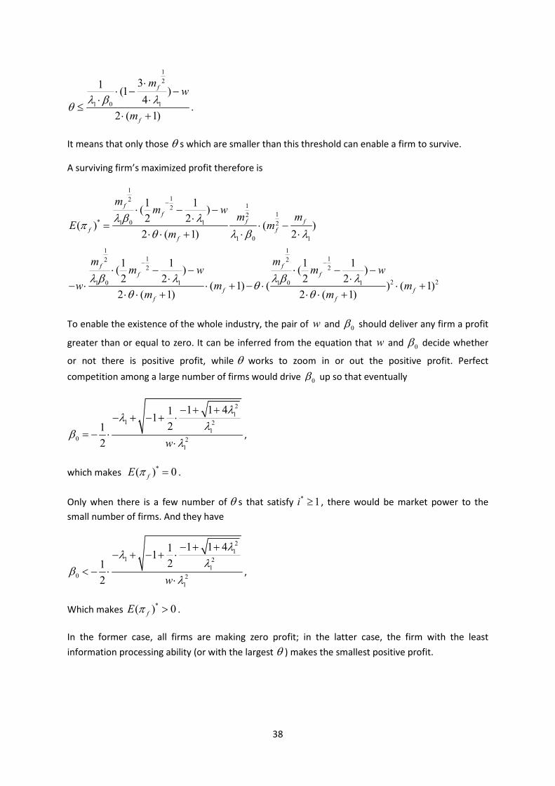
38

12

1 0 1

31(1 )

42 ( 1)

f

f

mw

mλ β λ

θ

⋅⋅ − −

⋅ ⋅≤

⋅ +.

It means that only those θ s which are smaller than this threshold can enable a firm to survive.

A surviving firm’s maximized profit therefore is

112

1212

* 1 0 1 2

1 0 1

1 11 12 22 2

2 21 0 1 1 0 1

1 1( )2 2

( ) ( )2 ( 1) 2

1 1 1 1( ) ( )2 2 2 2

( 1) ( ) ( 1)2 ( 1) 2 ( 1)

ff

f ff f

f

f ff f

f ff f

mm w

m mE m

m

m mm w m w

w m mm m

λ β λπ

θ λ β λ

λ β λ λ β λθ

θ θ

−

− −

⋅ − −⋅

= ⋅ −⋅ ⋅ + ⋅ ⋅

⋅ − − ⋅ − −⋅ ⋅

− ⋅ ⋅ + − ⋅ ⋅ +⋅ ⋅ + ⋅ ⋅ +

To enable the existence of the whole industry, the pair of w and 0β should deliver any firm a profit

greater than or equal to zero. It can be inferred from the equation that w and 0β decide whether

or not there is positive profit, while θ works to zoom in or out the positive profit. Perfect

competition among a large number of firms would drive 0β up so that eventually

21

1 21

0 21

1 1 411

212 w

λλ

λβ

λ

− + +− + − + ⋅

= − ⋅⋅

,

which makes *( ) 0fE π = .

Only when there is a few number of θ s that satisfy * 1i ≥ , there would be market power to the small number of firms. And they have

21

1 21

0 21

1 1 411

212 w

λλ

λβ

λ

− + +− + − + ⋅

< − ⋅⋅

,

Which makes *( ) 0fE π > .

In the former case, all firms are making zero profit; in the latter case, the firm with the least

information processing ability (or with the largest θ ) makes the smallest positive profit.

39

Figure 1

Figure 2

* 0 which overlaps with XA X

A

IU x Q x

Qβ⋅

= ⋅ =

( , )XAQ x

x

XAQ

40

Figure 3

Figure 4

41

Figure 5

Figure 6

42

Figure 7

Figure 9

3

2

1

θ ↓

More firm entry

Larger firm size

0 β ↑ (Intensity of competition)

wage ↑ (Stringent labor market)

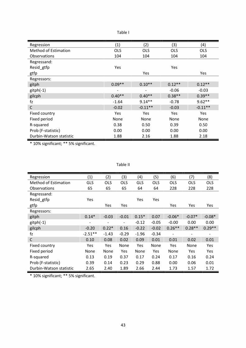
43

Table I

Regression (1) (2) (3) (4) Method of Estimation OLS OLS OLS OLS Observations 104 104 104 104 Regressand: Resid_gtfp Yes Yes gtfp Yes Yes Regressors: gitph 0.09** 0.10** 0.12** 0.12** gitph(-1) - - -0.06 -0.03 gilcph 0.40** 0.40** 0.38** 0.39** fz -1.64 9.14** -0.78 9.62** C -0.02 -0.11** -0.03 -0.11** Fixed country Yes Yes Yes Yes Fixed period None None None None R-squared 0.38 0.50 0.39 0.50 Prob (F-statistic) 0.00 0.00 0.00 0.00 Durbin-Watson statistic 1.88 2.16 1.88 2.18

* 10% significant; ** 5% significant.

Table II

Regression (1) (2) (3) (4) (5) (6) (7) (8) Method of Estimation GLS OLS OLS GLS OLS OLS OLS OLS Observations 65 65 65 64 64 228 228 228 Regressand: Resid_gtfp Yes Yes Yes gtfp Yes Yes Yes Yes Yes Regressors: gitph 0.14* -0.03 -0.01 0.15* 0.07 -0.06* -0.07* -0.08* gitph(-1) - - - -0.12 -0.05 -0.00 0.00 0.00 gilcph -0.20 0.22* 0.16 -0.22 -0.02 0.26** 0.28** 0.29** fz -2.51** -1.43 -0.29 -1.96 -0.34 - - - C 0.10 0.08 0.02 0.09 0.01 0.01 0.02 0.01 Fixed country Yes Yes None Yes None Yes None Yes Fixed period None None Yes None Yes None Yes Yes R-squared 0.13 0.19 0.37 0.17 0.24 0.17 0.16 0.24 Prob (F-statistic) 0.39 0.14 0.23 0.29 0.88 0.00 0.06 0.01 Durbin-Watson statistic 2.65 2.40 1.89 2.66 2.44 1.73 1.57 1.72

* 10% significant; ** 5% significant.

44

0

0.02

0.04

0.06

0.08

0.1

0.12

0 0.02 0.04 0.06 0.08 0.1 0.12

Stan

dard

dev

iati

on

Mean

ws_gilcph

UK

USA

JPN

GER

ITA

AUS

KOR

DNK

FIN

0

0.02

0.04

0.06

0.08

0.1

0.12

0 0.05 0.1 0.15 0.2

Stan

dard

dev

iati

on

Mean

ws_gitph

UK

USA

JPN

GER

ITA

AUS

KOR

DNK

FIN

0

0.005

0.01

0.015

0.02

0.025

0.03

0 0.005 0.01 0.015

Stan

dard

dev

iati

on

Mean

ws_glq

UK

USA

JPN

GER

ITA

AUS

KOR

DNK

FIN

00.010.020.030.040.050.060.070.080.09

0 0.02 0.04 0.06 0.08 0.1St

anda

rd d

evia

tion

Mean

ws_glph

UK

USA

JPN

GER

ITA

AUS

KOR

DNK

FIN

Figure 8: Key variables of the Wholesale and retail industry.

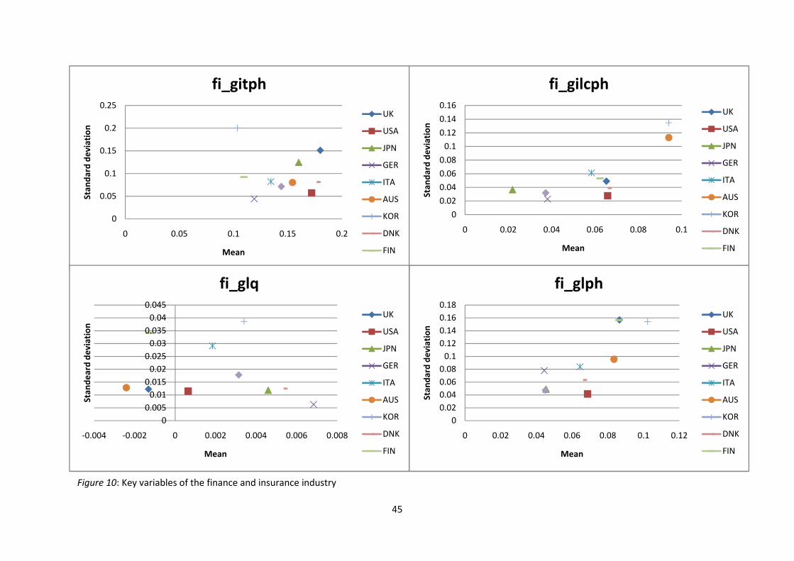
45

00.020.040.060.08

0.10.120.140.160.18

0 0.02 0.04 0.06 0.08 0.1 0.12St

anda

rd d

evia

tion

Mean

fi_glph

UK

USA

JPN

GER

ITA

AUS

KOR

DNK

FIN

0

0.05

0.1

0.15

0.2

0.25

0 0.05 0.1 0.15 0.2

Stan

dard

dev

iati

on

Mean

fi_gitph

UK

USA

JPN

GER

ITA

AUS

KOR

DNK

FIN

0

0.020.04

0.060.08

0.10.12

0.14

0.16

0 0.02 0.04 0.06 0.08 0.1

Stan

dard

dev

iati

on

Mean

fi_gilcph

UK

USA

JPN

GER

ITA

AUS

KOR

DNK

FIN

00.005

0.010.015

0.020.025

0.030.035

0.040.045

-0.004 -0.002 0 0.002 0.004 0.006 0.008

Stan

dear

d de

viat

ion

Mean

fi_glq

UK

USA

JPN

GER

ITA

AUS

KOR

DNK

FIN

Figure 10: Key variables of the finance and insurance industry