endogenous selection bias: the problem of · pdf fileendogenous selection bias: the problem of...

SO40CH02-WinshipElwert ARI 26 May 2014 20:19

RE V I E W

S

IN

A D V A

NC

E

Endogenous Selection Bias:The Problem of Conditioningon a Collider VariableFelix Elwert1 and Christopher Winship2

1Department of Sociology, University of Wisconsin, Madison, Wisconsin 53706;email: [email protected] of Sociology, Harvard University, Cambridge, Massachusetts 02138;email: [email protected]

Annu. Rev. Sociol. 2014. 40:2.1–2.23

The Annual Review of Sociology is online atsoc.annualreviews.org

This article’s doi:10.1146/annurev-soc-071913-043455

Copyright c⃝ 2014 by Annual Reviews.All rights reserved

Keywordscausality, directed acyclic graphs, identification, confounding

AbstractEndogenous selection bias is a central problem for causal inference. Rec-ognizing the problem, however, can be difficult in practice. This articleintroduces a purely graphical way of characterizing endogenous selec-tion bias and of understanding its consequences (Hernan et al. 2004).We use causal graphs (direct acyclic graphs, or DAGs) to highlight thatendogenous selection bias stems from conditioning (e.g., controlling,stratifying, or selecting) on a so-called collider variable, i.e., a variablethat is itself caused by two other variables, one that is (or is associatedwith) the treatment and another that is (or is associated with) the out-come. Endogenous selection bias can result from direct conditioning onthe outcome variable, a post-outcome variable, a post-treatment vari-able, and even a pre-treatment variable. We highlight the differencebetween endogenous selection bias, common-cause confounding, andovercontrol bias and discuss numerous examples from social stratifi-cation, cultural sociology, social network analysis, political sociology,social demography, and the sociology of education.

2.1

Review in Advance first posted online on June 2, 2014. (Changes may still occur before final publication online and in print.)

Changes may still occur before final publication online and in print

Ann

u. R

ev. S

ocio

l. 20

14.4

0. D

ownl

oade

d fro

m w

ww

.ann

ualre

view

s.org

by U

nive

rsity

of W

iscon

sin -

Mad

ison

on 0

7/11

/14.

For

per

sona

l use

onl

y.


Endogenousselection bias: thistype of bias resultsfrom conditioning on acollider (or itsdescendant) on anoncausal path linkingtreatment andoutcome

Conditioning:introducinginformation about avariable into ananalysis, e.g., viasample selection,stratification,regression control

Collider variable:a common outcome oftwo other variablesalong a path; collidersare path-specific

Common-causeconfounding bias:this type of bias resultsfrom failure tocondition on acommon cause oftreatment andoutcome

Identification:the possibility ofrecovering a causaleffect from ideal datagenerated by theassumed datagenerating process

Overcontrol bias:this type of bias resultsfrom conditioning on avariable on a causalpath betweentreatment andoutcome

1. INTRODUCTIONA large literature in economics, sociology, epi-demiology, and statistics deals with sample se-lection bias. Sample selection bias occurs whenthe selection of observations into a sample is notindependent of the outcome (Winship & Mare1992, p. 328). For example, estimates of the ef-fect of education on wages will be biased if thesample is restricted to low earners (Hausman& Wise 1977), and estimates for the effect ofmotherhood on wages will be biased if the sam-ple is restricted to employed women (Gronau1974, Heckman 1974).

Surveys of sample selection bias in sociologytend to emphasize examples where selectionis affected by the treatment or the outcome,i.e., where sample selection occurs aftertreatment (Berk 1983, Winship & Mare 1992,Stolzenberg & Relles 1997, Fu et al. 2004). Theunderlying problem, which we call endogenousselection bias, is more general than this, how-ever, in two respects. First, bias can also arise ifsample selection occurs prior to treatment. Sec-ond, bias can occur from simple conditioning(e.g., controlling or stratifying) on certain vari-ables even if no observations are discarded fromthe population (i.e., if no sample is selected).

Recognizing endogenous selection bias canbe difficult, especially when sample selectionoccurs prior to treatment or when no selec-tion (in the sense of discarding observations)takes place. This article introduces sociologiststo a new, purely graphical, way of character-izing endogenous selection bias that subsumesall of these scenarios. The goal is to facilitaterecognition of the problem in its many formsin practice. In contrast to previous surveys,which primarily draw on algebraic formulationsfrom econometrics, our presentation draws ongraphical approaches from computer science(Pearl 1995, 2009, 2010) and epidemiology(Greenland et al. 1999a, and especially Hernanet al. 2004). This paper makes five points:

First, we present a definition of endogenousselection bias. Endogenous selection biasresults from conditioning on an endogenousvariable that is caused by two other variables,

one that is (or is associated with) the treatmentand one that is (or is associated with) theoutcome (Hernan et al. 2002, 2004). In thegraphical approach introduced below, suchendogenous variables are called collidervariables. Collider variables may occur beforeor after the treatment and before or after theoutcome.1

Second, we describe the difference betweenconfounding, or omitted variable bias, andendogenous selection bias (Pearl 1995;Greenland et al. 1999a; Hernan et al. 2002,2004). Confounding originates from commoncauses, whereas endogenous selection origi-nates from common outcomes. Confoundingbias results from failing to control for acommon cause variable that one should havecontrolled for, whereas endogenous selectionbias results from controlling for a commonoutcome variable that one should not havecontrolled for.Third, we highlight the importance of en-dogenous selection bias for causal inferenceby noting that all nonparametric identifica-tion problems can be classified as one of threeunderlying problems: overcontrol bias, con-founding bias, and endogenous selection bias.Endogenous selection captures the commonstructure of a large number of biases usu-ally known by different names, including se-lective nonresponse, ascertainment bias, attri-tion bias, informative censoring, Heckman se-lection bias, sample selection bias, homophilybias, and others.Fourth, we illustrate that the commonplaceadvice not to select (i.e., condition) on thedependent variable of an analysis is too nar-row. Endogenous selection bias can originatein many places. Endogenous selection can

1We avoid the simpler term “selection bias” because it hasmultiple meanings across literatures. “Endogenous selectionbias” as defined in Section 4 of this article encompasses“sample selection bias” from econometrics (Vella 1998) and“Berkson’s (1946) bias” and “M-bias” (Greenland 2003) fromepidemiology. Our definition is identical to those of “col-lider stratification bias” (Greenland 2003), “selection bias”(Hernan et al. 2004), “explaining away effect” (Kim & Pearl1983), and “conditioning bias” (Morgan & Winship 2007).

2.2 Elwert ·Winship


Ann

u. R

ev. S

ocio

l. 20

14.4

0. D

ownl

oade

d fro

m w

ww

.ann

ualre

view

s.org

by U

nive

rsity

of W

iscon

sin -

Mad

ison

on 0

7/11

/14.

For

per

sona

l use

onl

y.


Direct acyclic graph(DAG): a graphicalrepresentation of thecausal assumptions inthe data generatingprocess

result from conditioning on an outcome,but it can also result from conditioning onvariables that have been affected by the out-come, variables that temporally precede theoutcome, and even variables that temporallyprecede the treatment (Greenland 2003).Fifth, and perhaps most importantly, we illus-trate the ubiquity of endogenous selection biasby reviewing numerous examples from stratifi-cation research, cultural sociology, social net-work analysis, political sociology, social de-mography, and the sociology of education.

The specific methodological points ofthis paper have been made before in variousplaces in econometrics, statistics, biostatistics,and computer science. Our innovation liesin offering a unified graphical presentationof these points for sociologists. Specifically,our presentation relies on direct acyclicgraphs (DAGs) (Pearl 1995, 2009; Elwert2013), a generalization of conventional linearpath diagrams (Wright 1934, Blalock 1964,Duncan 1966, Bollen 1989) that is entirelynonparametric (making no distributional orfunctional form assumptions).2 DAGs areformally rigorous yet accessible because theyrely on graphical rules instead of algebra. Wehope that this presentation may empower evensociologists with little mathematical training torecognize and understand precisely when andwhy endogenous selection bias may trouble anempirical investigation.

We begin by reviewing the required tech-nical material. Section 2 describes the notionof nonparametric identification. Section 3introduces DAGs. Section 4 explains thethree structural sources of association betweentwo variables—causation, confounding, andendogenous selection—and describes howDAGs can be used to distinguish causalassociations from spurious associations. Sec-tion 5—the heart of this article—examines a

2The equivalence of DAGs and nonparametric structuralequation models is discussed in Pearl (2009, 2010). The rela-tionship between DAGs and conventional structural equationmodels is discussed by Bollen & Pearl (2013).

large number of applied examples in whichendogenous selection is a problem. Section6 concludes by reflecting on dealing withendogenous selection bias in practice.

2. IDENTIFICATION VERSUSESTIMATIONWe investigate endogenous selection biasas a problem for the identification of causaleffects. Following the modern literature oncausal inference, we define causal effects ascontrasts between potential outcomes (Rubin1974, Morgan & Winship 2007). Recoveringcausal effects from data is difficult becausecausal effects can never be observed directly(Holland 1986). Rather, causal effects have tobe inferred from observed associations, whichare generally a mixture of the desired causaleffect and various noncausal, or spurious,components. Neatly dividing associations intotheir causal and spurious components is thetask of identification analysis. A causal effect issaid to be identified if it is possible, with idealdata (infinite sample size and no measurementerror), to purge an observed association ofall noncausal components such that only thecausal effect of interest remains.

Identification analysis requires a theory(i.e., a model or assumptions) of how the datawere generated. Consider, for example, theidentification of the causal effect of educationon wages. If one assumes that ability positivelyinfluences both education and wages, then theobserved marginal (i.e., unadjusted) associationbetween education and wages does not identifythe causal effect of education on wages. But ifone can assume that ability is the only factorinfluencing both education and wages, then theconditional association between education andwages after perfectly adjusting for ability wouldidentify the causal effect of education on wages.Unfortunately, the analyst’s theory of datageneration can never be fully tested empirically(Robins & Wasserman 1999). Therefore, itis important that the analyst’s theory of datageneration is stated explicitly for other scholars

www.annualreviews.org • Endogenous Selection Bias 2.3


Ann

u. R

ev. S

ocio

l. 20

14.4

0. D

ownl

oade

d fro

m w

ww

.ann

ualre

view

s.org

by U

nive

rsity

of W

iscon

sin -

Mad

ison

on 0

7/11

/14.

For

per

sona

l use

onl

y.


to inspect and judge. We use DAGs to clearlystate the data-generating model.

Throughout, we focus on nonparametricidentification, i.e., identification results thatcan be established solely from qualitative causalassumptions about the data-generating processwithout relying on parametric assumptionsabout the distribution of variables (e.g., jointnormality) or the functional form of causaleffects (e.g., linearity). We consider thisnonparametric focus an important strengthbecause cause-effect statements are claimsabout social reality that sociologists dealwith on a daily basis, whereas distributionaland functional form assumptions often lacksociological justification.

Identification (assuming ideal data) is anecessary precondition for unbiased estimation(with real data). Because there is, at present,no universal solution to estimating causaleffects in the presence of endogenous selection(Stolzenberg & Relles 1997, p. 495), we focushere on identification and deal with estimationonly in passing. Reviews of the large economet-ric literature on estimating causal effects undervarious scenarios of endogenous selection canbe found in Pagan & Ullah (1997), Vella (1998),Grasdal (2001), and Christofides et al. (2003),which cover Hausman & Wise’s (1977) trun-cated regression models and Heckman’s (1976,1979) classic two-step estimator, as well as nu-merous extensions. Bareinboim & Pearl (2012)discuss estimation under endogenous selectionwithin the graphical framework adopted here.A growing literature in epidemiology and bio-statistics builds on Robins (1986, 1994, 1999)to deal with the endogenous selection problemsthat occur with time-varying treatments.

3. DAGs IN BRIEF3

DAGs encode the analyst’s qualitative causalassumptions about the data-generating process

3This and the following section draw on Elwert’s (2013) sur-vey of DAGs for social scientists.

X T C Y

U

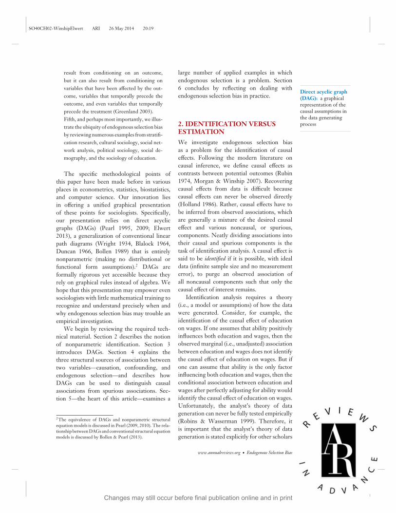
Figure 1A directed acyclic graph (DAG).

in the population (thus abstracting from sam-pling variability; see Pearl 2009 for technicaldetails). Collectively, these assumptions com-prise the model, or theory, on which the analystcan base her identification analysis. DAGsconsist of three elements (Figure 1). First, let-ters represent random variables, which may beobserved or unobserved. Variables can have anydistribution (continuous or discrete). Second,arrows represent direct causal effects.4 Directeffects may have any functional form (linear ornonlinear), they may differ in magnitude acrossindividuals (effect heterogeneity), and—withincertain constraints (Elwert 2013)—they mayvary with the value of other variables (effectinteraction or modification). Because the futurecannot cause the past, the arrows order pairsof variables in time such that DAGs do notcontain directed cycles. Third, missing arrowsrepresent the sharp assumption of no causaleffect between variables. In the parlance ofeconomics, missing arrows represent exclusionrestrictions. For example, Figure 1 excludesthe arrows U→T and X→Y, among others.Missing arrows are essential for inferringcausal information from data.

For clarity, and without infringing upon ourconceptual points, we assume that the DAGsin this review display all observed and unob-served common causes in the process underinvestigation. Note that this assumption im-plies that all other inputs into variables must be

4Strictly speaking, arrows represent possible (rather than cer-tain) causal effects (see Elwert 2013). This distinction is notimportant for the purposes of this paper and we neglect itbelow.



Ann

u. R

ev. S

ocio

l. 20

14.4

0. D

ownl

oade

d fro

m w

ww

.ann

ualre

view

s.org

by U

nive

rsity

of W

iscon

sin -

Mad

ison

on 0

7/11

/14.

For

per

sona

l use

onl

y.


Path: a sequence ofarrows linking twovariables regardless ofthe direction of thearrows

Causal path: a pathlinking treatment andoutcome where allarrows point awayfrom the treatmentand toward theoutcome

Noncausal path: apath linking treatmentand outcome that isnot a causal path

marginally independent, i.e., all variables haveindependent error terms. These independenterror terms need not be displayed in the DAGbecause they never help nonparametric iden-tification (we occasionally display them belowwhen they harm identification).

A path is a sequence of arrows connect-ing two variables regardless of the direction ofthe arrowheads. A path may traverse a givenvariable at most once. A causal path betweentreatment and outcome is a path in which all ar-rows point away from the treatment and towardthe outcome. Assessing existence and magni-tude of causal paths is the task of causal test-ing and causal estimation, respectively. The setof all causal paths between a treatment and anoutcome comprise the total causal effect. Un-less specifically stated otherwise, this review isconcerned with the identification of average to-tal causal effects in the data represented by theDAG. In Figure 1, the total causal effect ofT on Y comprises the causal paths T→Y andT→C→Y. All other paths between treatmentand outcome are called noncausal (or spurious)paths, e.g., T→C←U→Y and T←X←U→Y.

If two arrows along a path both point directlyinto the same variable, the variable is called acollider variable on the path (collider, for short).Otherwise, the variable is called a noncollideron the path. Note that the same variable maybe a collider on one path and a noncollider onanother path. In Figure 1, C is a collider on thepath T→C←U and a noncollider on the pathT→C→Y.

We make extensive reference to condition-ing on a variable. Most broadly, conditioningrefers to introducing information about avariable into the analysis by some means. Insociology, conditioning usually takes the formof controlling for a variable in a regressionmodel, but it could also take the form ofstratifying on a variable, performing a group-specific analysis (thus conditioning on groupmembership), or collecting data selectively(e.g., excluding children, prisoners, retirees,or nonrespondents from a survey). We denoteconditioning graphically by drawing a boxaround the conditioned variable.

a bA C B A C B

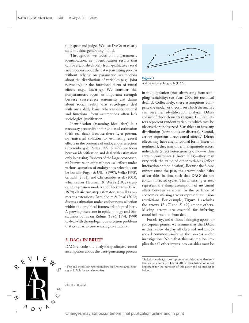
Figure 2(a) A and B are associated by causation. The marginal association between Aand B identifies the causal effect of A on B. (b) A and B are conditionallyindependent given C. The conditional association between A and B given Cdoes not identify the causal effect of A on B (overcontrol bias).

4. SOURCES OF ASSOCIATION:CAUSATION, CONFOUNDING,AND ENDOGENOUS SELECTION

The Building Blocks: Causation,Confounding, and EndogenousSelection

The power of DAGs lies in their ability to re-veal all marginal and conditional associationsand independences implied by a qualitativecausal model (Pearl 2009). This enables the an-alyst to discern which observable associationsare solely causal and which ones are not—inother words, to conduct a formal nonparamet-ric identification analysis. Absent sampling vari-ation (i.e., chance), all observable associationsoriginate from just three elementary configu-rations: chains (A→B, A→C→B, etc.), forks(A←C→B), and inverted forks (A→C←B)(Pearl 1988, 2009; Verma & Pearl 1988). Con-veniently, these three configurations corre-spond exactly to the sources of causation, con-founding bias, and endogenous selection bias.5

First, two variables are associated if one vari-able directly or indirectly causes the other. InFigure 2a, A indirectly causes B via C. Indata generated according to this DAG, the ob-served marginal association between A and Bwould reflect pure causation—in other words,the marginal association between A and B iden-tifies the causal effect of A on B. By contrast,conditioning on the intermediate variable C in

5Deriving the associational implications of causal structuresrequires two mild assumptions not discussed here, knownas causal Markov assumption and faithfulness. See Glymour& Greenland (2008) for a nontechnical summary. See Pearl(2009) and Spirtes et al. (2000) for details.



Ann

u. R

ev. S

ocio

l. 20

14.4

0. D

ownl

oade

d fro

m w

ww

.ann

ualre

view

s.org

by U

nive

rsity

of W

iscon

sin -

Mad

ison

on 0

7/11

/14.

For

per

sona

l use

onl

y.


a A b A

C C

B B

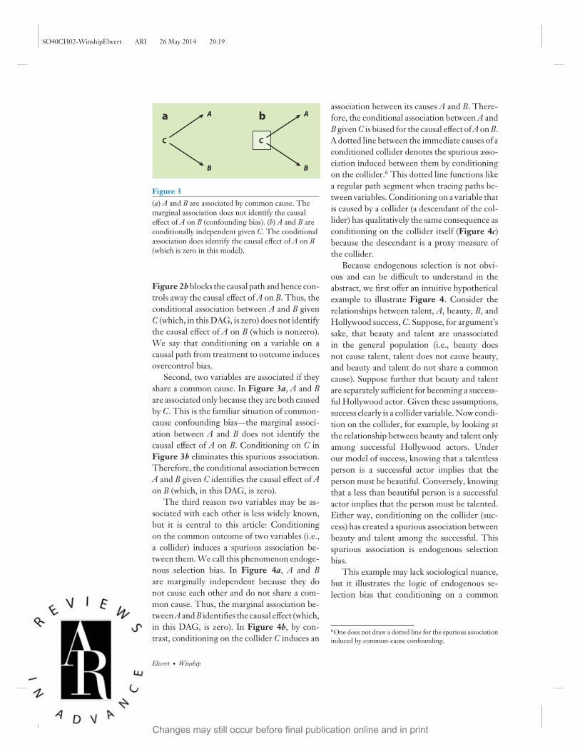
Figure 3(a) A and B are associated by common cause. Themarginal association does not identify the causaleffect of A on B (confounding bias). (b) A and B areconditionally independent given C. The conditionalassociation does identify the causal effect of A on B(which is zero in this model).

Figure 2b blocks the causal path and hence con-trols away the causal effect of A on B. Thus, theconditional association between A and B givenC (which, in this DAG, is zero) does not identifythe causal effect of A on B (which is nonzero).We say that conditioning on a variable on acausal path from treatment to outcome inducesovercontrol bias.

Second, two variables are associated if theyshare a common cause. In Figure 3a, A and Bare associated only because they are both causedby C. This is the familiar situation of common-cause confounding bias—the marginal associ-ation between A and B does not identify thecausal effect of A on B. Conditioning on C inFigure 3b eliminates this spurious association.Therefore, the conditional association betweenA and B given C identifies the causal effect of Aon B (which, in this DAG, is zero).

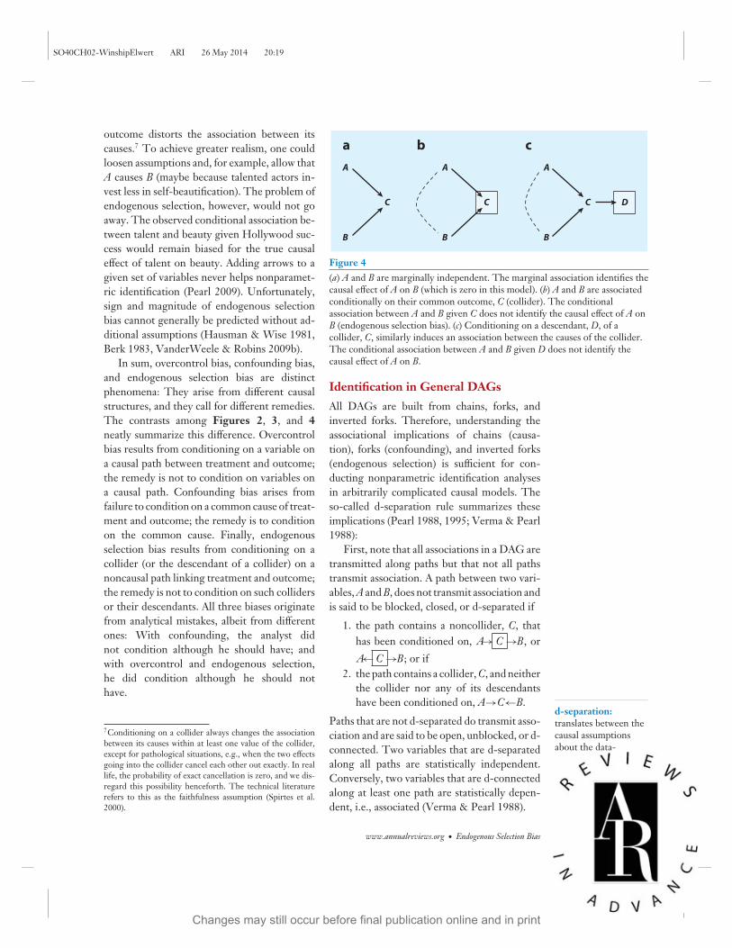
The third reason two variables may be as-sociated with each other is less widely known,but it is central to this article: Conditioningon the common outcome of two variables (i.e.,a collider) induces a spurious association be-tween them. We call this phenomenon endoge-nous selection bias. In Figure 4a, A and Bare marginally independent because they donot cause each other and do not share a com-mon cause. Thus, the marginal association be-tween A and B identifies the causal effect (which,in this DAG, is zero). In Figure 4b, by con-trast, conditioning on the collider C induces an

association between its causes A and B. There-fore, the conditional association between A andB given C is biased for the causal effect of A on B.A dotted line between the immediate causes of aconditioned collider denotes the spurious asso-ciation induced between them by conditioningon the collider.6 This dotted line functions likea regular path segment when tracing paths be-tween variables. Conditioning on a variable thatis caused by a collider (a descendant of the col-lider) has qualitatively the same consequence asconditioning on the collider itself (Figure 4c)because the descendant is a proxy measure ofthe collider.

Because endogenous selection is not obvi-ous and can be difficult to understand in theabstract, we first offer an intuitive hypotheticalexample to illustrate Figure 4. Consider therelationships between talent, A, beauty, B, andHollywood success, C. Suppose, for argument’ssake, that beauty and talent are unassociatedin the general population (i.e., beauty doesnot cause talent, talent does not cause beauty,and beauty and talent do not share a commoncause). Suppose further that beauty and talentare separately sufficient for becoming a success-ful Hollywood actor. Given these assumptions,success clearly is a collider variable. Now condi-tion on the collider, for example, by looking atthe relationship between beauty and talent onlyamong successful Hollywood actors. Underour model of success, knowing that a talentlessperson is a successful actor implies that theperson must be beautiful. Conversely, knowingthat a less than beautiful person is a successfulactor implies that the person must be talented.Either way, conditioning on the collider (suc-cess) has created a spurious association betweenbeauty and talent among the successful. Thisspurious association is endogenous selectionbias.

This example may lack sociological nuance,but it illustrates the logic of endogenous se-lection bias that conditioning on a common

6One does not draw a dotted line for the spurious associationinduced by common-cause confounding.



Ann

u. R

ev. S

ocio

l. 20

14.4

0. D

ownl

oade

d fro

m w

ww

.ann

ualre

view

s.org

by U

nive

rsity

of W

iscon

sin -

Mad

ison

on 0

7/11

/14.

For

per

sona

l use

onl

y.


d-separation:translates between thecausal assumptionsabout the data-generating process andobservable associations

outcome distorts the association between itscauses.7 To achieve greater realism, one couldloosen assumptions and, for example, allow thatA causes B (maybe because talented actors in-vest less in self-beautification). The problem ofendogenous selection, however, would not goaway. The observed conditional association be-tween talent and beauty given Hollywood suc-cess would remain biased for the true causaleffect of talent on beauty. Adding arrows to agiven set of variables never helps nonparamet-ric identification (Pearl 2009). Unfortunately,sign and magnitude of endogenous selectionbias cannot generally be predicted without ad-ditional assumptions (Hausman & Wise 1981,Berk 1983, VanderWeele & Robins 2009b).

In sum, overcontrol bias, confounding bias,and endogenous selection bias are distinctphenomena: They arise from different causalstructures, and they call for different remedies.The contrasts among Figures 2, 3, and 4neatly summarize this difference. Overcontrolbias results from conditioning on a variable ona causal path between treatment and outcome;the remedy is not to condition on variables ona causal path. Confounding bias arises fromfailure to condition on a common cause of treat-ment and outcome; the remedy is to conditionon the common cause. Finally, endogenousselection bias results from conditioning on acollider (or the descendant of a collider) on anoncausal path linking treatment and outcome;the remedy is not to condition on such collidersor their descendants. All three biases originatefrom analytical mistakes, albeit from differentones: With confounding, the analyst didnot condition although he should have; andwith overcontrol and endogenous selection,he did condition although he should nothave.

7Conditioning on a collider always changes the associationbetween its causes within at least one value of the collider,except for pathological situations, e.g., when the two effectsgoing into the collider cancel each other out exactly. In reallife, the probability of exact cancellation is zero, and we dis-regard this possibility henceforth. The technical literaturerefers to this as the faithfulness assumption (Spirtes et al.2000).

a b cA A A

C C DC

B B B

Figure 4(a) A and B are marginally independent. The marginal association identifies thecausal effect of A on B (which is zero in this model). (b) A and B are associatedconditionally on their common outcome, C (collider). The conditionalassociation between A and B given C does not identify the causal effect of A onB (endogenous selection bias). (c) Conditioning on a descendant, D, of acollider, C, similarly induces an association between the causes of the collider.The conditional association between A and B given D does not identify thecausal effect of A on B.

Identification in General DAGsAll DAGs are built from chains, forks, andinverted forks. Therefore, understanding theassociational implications of chains (causa-tion), forks (confounding), and inverted forks(endogenous selection) is sufficient for con-ducting nonparametric identification analysesin arbitrarily complicated causal models. Theso-called d-separation rule summarizes theseimplications (Pearl 1988, 1995; Verma & Pearl1988):

First, note that all associations in a DAG aretransmitted along paths but that not all pathstransmit association. A path between two vari-ables, A and B, does not transmit association andis said to be blocked, closed, or d-separated if

1. the path contains a noncollider, C, thathas been conditioned on, A→ C →B, orA← C →B; or if

2. the path contains a collider, C, and neitherthe collider nor any of its descendantshave been conditioned on, A→C←B.

Paths that are not d-separated do transmit asso-ciation and are said to be open, unblocked, or d-connected. Two variables that are d-separatedalong all paths are statistically independent.Conversely, two variables that are d-connectedalong at least one path are statistically depen-dent, i.e., associated (Verma & Pearl 1988).



Ann

u. R

ev. S

ocio

l. 20

14.4

0. D

ownl

oade

d fro

m w

ww

.ann

ualre

view

s.org

by U

nive

rsity

of W

iscon

sin -

Mad

ison

on 0

7/11

/14.

For

per

sona

l use

onl

y.


Importantly, conditioning on a variable hasopposite consequences depending on whetherthe variable is a collider or a noncollider: Con-ditioning on a noncollider blocks the flow ofassociation along a path, whereas conditioningon a collider opens the flow of association.

One can then determine the identifiabilityof a causal effect by checking whether one canblock all noncausal paths between treatmentand outcome without blocking any causal pathsbetween treatment and outcome by condition-ing on a suitable set of observed variables.8 Forexample, in Figure 1, the total causal effect of Ton Y can be identified by conditioning on X be-cause X does not sit on a causal path from T to Yand conditioning on X blocks the two noncausalpaths between T and Y, T← X ←U→Y andT← X ←U→C→Y , that would otherwise beopen. (A third noncausal path between T and Y,T→C←U→Y, is unconditionally blocked be-cause it contains the collider C. Conditioningon C would ruin identification for two reasons:First, it would induce endogenous selection biasby opening the noncausal path T→ C ←U→Y ;second, it would induce overcontrol bias be-cause C sits on a causal path from T to Y,T→ C →Y .)

The motivation for this review is that it isall too easy to open noncausal paths betweentreatment and outcome inadvertently by con-ditioning on a collider, thus inducing endoge-nous selection bias. Examples of such bias insociology are discussed next.

5. EXAMPLES OF ENDOGENOUSSELECTION BIAS IN SOCIOLOGYEndogenous selection bias may originate fromconditioning on a collider at any point in acausal process. Endogenous selection bias canbe induced by conditioning on a collider that

8This is the logic of “identification by adjustment,” whichunderlies identification in regression and matching. Otheridentification strategies exist. Pearl’s do-calculus is a completenonparametric graphical identification criterion that includesall types of nonparametric identification as special cases (Pearl1995).

occurs after the outcome; by conditioning ona collider that is an intermediate variable be-tween the treatment and the outcome; and byconditioning on a collider that occurs beforethe treatment (Greenland 2003). Therefore, weorganize the following sociological examples ofendogenous selection bias according to the tim-ing of the collider relative to the treatment andthe outcome.

Conditioning on a (Post-) OutcomeColliderIt is well known that outright selection on theoutcome, as well as conditioning on a vari-able affected by the outcome, can lead to bias(e.g., Berkson 1946; Gronau 1974; Heckman1974, 1976, 1979). Nevertheless, both prob-lems continue to occur in empirical sociologicalresearch, where they may result from nonran-dom sampling schemes during data collectionor from seemingly compelling choices duringdata analysis. Here, we present canonical andmore recent examples, explicating them as en-dogenous selection bias due to conditioning ona collider.

Sample truncation bias. Hausman & Wise’s(1977) influential analysis of sample truncationbias furnishes a classic example of endogenousselection bias. They consider the problem ofestimating the effect of education on incomefrom a sample selected (truncated) to containonly low earners. Figure 5 describes the heartof the problem. Income, I, is affected by edu-cation, E, as well as by other factors tradition-ally subsumed in the error term, U. Assume,for clarity and without loss of generality, that Eand U are independent in the population (i.e.,share no common causes and do not cause eachother). Then the marginal association betweenE and I in the population would identify thecausal effect E→I. The DAG shows, however,that I is a collider variable on the path betweentreatment and the error term, E→I←U. Re-stricting the sample to low earners amounts toconditioning on this collider. As a result, thereare now two sources of association between Eand I: the causal path E→I, which represents the



Ann

u. R

ev. S

ocio

l. 20

14.4

0. D

ownl

oade

d fro

m w

ww

.ann

ualre

view

s.org

by U

nive

rsity

of W

iscon

sin -

Mad

ison

on 0

7/11

/14.

For

per

sona

l use

onl

y.


I

E

U

Figure 5Endogenous selection bias due to outcometruncation, with E as education (treatment), I asincome (outcome, truncated at 1.5 times povertythreshold), and U as error term on income.

causal effect of interest, and the newly inducednoncausal path E- - -U→I. Sample truncationhas induced endogenous selection bias so thatthe association between E and I in the truncatedsample does not identify the causal effect of Eon I.

This example illustrates an important gen-eral point: If a treatment, T, has an effect on theoutcome, Y, T→Y, then the outcome is a col-lider variable on the path between the treatmentand the outcome’s error term, U, T→Y←U.Therefore, outright selection on an outcome,or selection on a variable affected by the out-come, is always potentially problematic.

Nonresponse bias. The same causal structurethat leads to truncation bias also underlies non-response bias in retrospective studies, exceptthat nonresponse is better understood as con-ditioning on a variable affected by the outcomerather than conditioning on the outcome itself.Consider a simplified version of the examplediscussed by Lin et al. (1999), who investigatethe consequences of nonresponse for esti-mating the effect of divorced fathers’ incomeon their child support payments (Figure 6).A divorced father’s income, I, and the amountof child support he pays, P, both influencewhether a father responds to the study, R.(Without loss of generality, we neglect that Iand P may share common causes.) Responsebehavior is thus a collider along a non-causal path between treatment and outcome,I→R←P. Analyzing only completed interviewsby dropping nonresponding fathers (listwisedeletion) amounts to conditioning on this

R

I

P

Figure 6Endogenous selection bias due to listwise deletion[I, father’s income (treatment); P, child supportpayments (outcome); R, survey response].Conditioning on the post-outcome variableresponse behavior R (listwise deletion of missingdata) induces a noncausal association betweenfather’s income, I, and his child support payments, P.

collider, which induces a noncausal associationbetween fathers’ income and the child supportthey pay, i.e., endogenous selection bias.

Ascertainment bias. Sociological research onelite achievement sometimes employs nonran-dom samples when collecting data on the en-tire population is too expensive or drawing arandom sample is infeasible. Such studies maysample all individuals, organizations, or culturalproducts that have achieved a certain elite status(e.g., sitting on the Supreme Court, qualifyingfor the Fortune 500, or receiving critical acco-lades) and a control group of individuals, orga-nizations, or cultural products that have distin-guished themselves in some other manner (e.g.,sitting on the federal bench, posting revenuesin excess of $100 million, or being commer-cially successful). The logic of this approach isto compare the most outstandingly successfulcases to somewhat less outstandingly success-ful cases in order to understand what sets themapart. The problem is that studying the causesof success in a sample selected for success invitesendogenous selection bias.

We suspect that this sampling strategy mayaccount for a surprising recent finding aboutthe determinants of critical success in the musicindustry (Schmutz 2005; see also Allen & Lin-coln 2004, Schmutz & Faupel 2010). The studyaimed, among other goals, to identify the effectsof a music album’s commercial success on itschances of inclusion in Rolling Stone magazine’s



Ann

u. R

ev. S

ocio

l. 20

14.4

0. D

ownl

oade

d fro

m w

ww

.ann

ualre

view

s.org

by U

nive

rsity

of W

iscon

sin -

Mad

ison

on 0

7/11

/14.

For

per

sona

l use

onl

y.


S

B

R

Figure 7Endogenous selection bias due to sample selection[B, topping the Billboard charts (treatment); R,inclusion in the Rolling Stone 500 (outcome); S,sample selection].

vaunted list of 500 Greatest Albums of All Time.The sample included roughly 1,700 albums: allalbums in the Rolling Stone 500 and 1,200 ad-ditional albums, all of which had earned someother elite distinction, such as topping the Bill-board charts or winning a critics’ poll. Amongthe tens of thousands of albums released inthe United States over the decades, the 1,700sampled albums clearly represent a subset thatis heavily selected for success. A priori, onemight expect that outstanding commercial suc-cess (i.e., topping the Billboard charts) shouldincrease an album’s chances of inclusion in theRolling Stone 500 (because the experts compil-ing the list can only consider albums that theyknow, probably know all chart toppers, andcannot possibly know all albums ever released).Surprisingly, however, a logistic regression ofthe analytic sample indicated that topping theBillboard charts was strongly negatively asso-ciated with inclusion in the Rolling Stone 500.

Why? As the authors noted, this resultshould be interpreted with caution (Schmutz2005, p. 1520; Schmutz & Faupel 2010, p. 705).We hypothesize that the finding is due to en-dogenous selection bias. The DAG in Figure 7illustrates the argument. (For clarity, we do notconsider additional explanatory variables in thestudy.) The outcome is an album’s inclusion inthe Rolling Stone 500, R. The treatment is top-ping the Billboard charts, B, which presumablyhas a positive effect on R in the population of allalbums. By construction, both R and B have astrong, strictly positive effect on inclusion in thesample, S. Analyzing this sample means that theanalysis conditions on inclusion in the sample,

Table 1 Simplified representation of thesampling scheme of a study of the effect oftopping the Billboard charts (B) on a record’sinclusion in the Rolling Stone 500 (R)

R = 0 R = 1a bc d

B = 0B = 1

S, which is a collider on a noncausal path be-tween treatment and outcome, B→S←R. Con-ditioning on this collider changes the associa-tion between its immediate causes, R and B, andinduces endogenous selection bias. If the sam-ple is sufficiently selective of the population ofall albums, then the bias may be large enoughto reverse the sign on the estimated effect of Bon R, producing a negative estimate for a causaleffect that may in fact be positive.

Table 1 makes the same point. For binaryB and R, B = 1 denotes topping the Billboardcharts, R = 1 denotes inclusion in the RollingStone 500, and 0 otherwise. The cell counts a,b, c, and d define the population of all albums.In the absence of common-cause confounding(as encoded in Figure 7), the population oddsratio ORP = ad/bc gives the true causal effectof B on R. Now note that most albums everreleased neither topped the charts nor won in-clusion in the Rolling Stone 500. To reduce thedata collection burden, the study then sampleson success by including all albums with R = 1and all albums with B = 1 in the analysis andseverely undersamples less successful albums,aS <a. The odds ratio from the logistic regres-sion of R on B in this selected sample wouldthen be downward biased compared with thetrue population odds ratio and possibly flipdirections, ORS = aSd/bc < ad/bc = ORP.

We note that the recovery of causal informa-tion despite direct selection on the outcome issometimes possible if certain constraints can beimposed on the data. This is the domain of theepidemiological literature on case-control stud-ies (Rothman et al. 2008) and the econometricliterature on response- or choice-based sam-pling (Manski 2003, ch. 6). A key rule in case-control studies, however, is that observations



Ann

u. R

ev. S

ocio

l. 20

14.4

0. D

ownl

oade

d fro

m w

ww

.ann

ualre

view

s.org

by U

nive

rsity

of W

iscon

sin -

Mad

ison

on 0

7/11

/14.

For

per

sona

l use

onl

y.


should not be sampled (ascertained) as a func-tion of both the treatment and the outcome.The consequence of violating this rule is knownas ascertainment bias (Rothman et al. 2008).The endogenous selection bias in the presentexample is ascertainment bias because controlalbums are sampled as a function of (a) exclu-sion from the Rolling Stone 500 and (b) commer-cial success. (Greenland et al. 1999 and Hernanet al. 2004 use DAGs to discuss ascertainmentbias as endogenous selection bias in a numberof interesting biomedical case-control studies.)

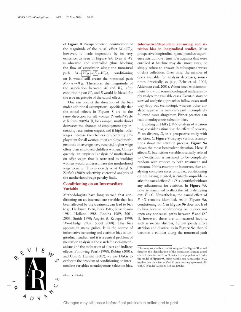
Heckman selection bias. Heckman selectionbias—perhaps the best-known selection bias inthe social sciences—can be explicated as en-dogenous selection bias. A classic example is theeffect of motherhood (i.e., having a child), M,on the wages offered to women by potential em-ployers, WO (Gronau 1974, Heckman 1974).Figure 8 displays the relevant DAGs. Follow-ing standard labor market theory, assume thatmotherhood will affect a woman’s reservationwage, WR, i.e., the wage that would be nec-essary to draw her out of the home and intothe workforce. Employment, E, is a functionboth of the wage offer and the reservation wagebecause a woman will only accept the job ifthe wage offer meets or exceeds her reserva-tion wage. Therefore, employment is a collideron the path M→WR→E←WO between moth-erhood and offer wages. (For simplicity, assumethat M and WO share no common cause.)

Many social science data sets include in-formation on motherhood, M, but they typi-cally do not include information on women’sreservation wage, WR. Importantly, the datatypically include information on offer wages,WO, only for those women who are actuallyemployed. If the analyst restricts the analy-sis to employed women, he will thus con-dition on the collider E, unblock the non-causal path from motherhood to offer wages,M→WR→ E ←W O , and induce endogenousselection bias. The analysis would thus indicatean association between motherhood and wageseven if the causal effect of motherhood on wagesis in fact zero (Figure 8a).

E

a bM

ε

(WR)

WO

E

M

ε

(WR)

WO

Figure 8Endogenous selection bias due to sample selection [M, motherhood (treatment);WR, unobserved reservation wage; WO, offer wage (outcome); E, employment;ε, error term on offer wage]. (a) Null model without effect of motherhoodon offer wages. (b) Model with effect of motherhood on offer wages.

If motherhood has no effect on offer wages,as in Figure 8a, the endogenous selectionproblem is bad enough. Further complicationsare introduced by permitting the possibilitythat motherhood may indeed have an effecton offer wages (e.g., because of mothers’ dif-ferential productivity compared with childlesswomen or because of employer discrimina-tion). This is shown in Figure 8b by addingthe arrow M→WO. This slight modificationof the DAG creates a second endogenousselection problem. Given that, as noted above,all outcomes are colliders on the path betweentreatment and the error term if treatmenthas an effect on the outcome, conditioningon E now further amounts to conditioningon the descendant of the collider WO on thepath M→ WO ←ε. This induces a noncausalassociation between motherhood and the errorterm on offer wages, M- - -ε→WO. Note thatthis second—but not the first—endogenous se-lection problem persists even if the noncolliderWR is measured and controlled.

The distinction between these two en-dogenous selection problems affords a freshopportunity for nonparametric inference that,to our knowledge, has not yet been exploited inthe applied literature on the motherhood wagepenalty: The analyst could nonparametricallytest the causal null hypothesis of no effect ofmotherhood on offer wages by observing andcontrolling women’s reservation wages. If Mand WO are not associated after conditioningon WR and E, then there is no causal effect ofM on WO under the two competing models



Ann

u. R

ev. S

ocio

l. 20

14.4

0. D

ownl

oade

d fro

m w

ww

.ann

ualre

view

s.org

by U

nive

rsity

of W

iscon

sin -

Mad

ison

on 0

7/11

/14.

For

per

sona

l use

onl

y.


of Figure 8. Nonparametric identification ofthe magnitude of the causal effect M→WO,however, is made impossible by its veryexistence, as seen in Figure 8b: Even if WR

is observed and controlled (thus blockingthe flow of association along the noncausalpath M→ WR → E ←W O ), conditioningon E would still create the noncausal pathM- - -ε→WO. Therefore, the magnitude ofthe association between M and WO afterconditioning on WR and E would be biased forthe true magnitude of the causal effect.

One can predict the direction of the biasunder additional assumptions, specifically thatthe causal effects in Figure 8 are in thesame direction for all women (VanderWeele& Robins 2009b). If, for example, motherhooddecreases the chances of employment (by in-creasing reservation wages), and if higher offerwages increase the chances of accepting em-ployment for all women, then employed moth-ers must on average have received higher wageoffers than employed childless women. Conse-quently, an empirical analysis of motherhoodon offer wages that is restricted to workingwomen would underestimate the motherhoodwage penalty. This is exactly what Gangl &Ziefle’s (2009) selectivity-corrected analysis ofthe motherhood wage penalty finds.

Conditioning on an IntermediateVariableMethodologists have long warned that con-ditioning on an intermediate variable that hasbeen affected by the treatment can lead to bias(e.g., Heckman 1976; Berk 1983; Rosenbaum1984; Holland 1988; Robins 1989, 2001,2003; Smith 1990; Angrist & Krueger 1999;Wooldridge 2005; Sobel 2008). This biasappears in many guises. It is the source ofinformative censoring and attrition bias in lon-gitudinal studies, and it is a central problem ofmediation analysis in the search for social mech-anisms and the estimation of direct and indirecteffects. Following Pearl (1998), Robins (2001),and Cole & Hernan (2002), we use DAGs toexplicate the problem of conditioning on inter-mediate variables as endogenous selection bias.

Informative/dependent censoring and at-trition bias in longitudinal studies. Mostprospective longitudinal (panel) studies experi-ence attrition over time. Participants that wereenrolled at baseline may die, move away, orsimply refuse to answer in subsequent wavesof data collection. Over time, the number ofcases available for analysis decreases, some-times drastically so (e.g., Behr et al. 2005,Alderman et al. 2001). When faced with incom-plete follow up, some sociological analyses sim-ply analyze the available cases. Event-history orsurvival-analytic approaches follow cases untilthey drop out (censoring), whereas other an-alytic approaches may disregard incompletelyfollowed cases altogether. Either practice canlead to endogenous selection bias.

Building on Hill’s (1997) analysis of attritionbias, consider estimating the effect of poverty,P, on divorce, D, in a prospective study withattrition, C. Figure 9 displays various assump-tions about the attrition process. Figure 9ashows the most benevolent situation. Here, Paffects D, but neither variable is causally relatedto C—attrition is assumed to be completelyrandom with respect to both treatment andoutcome. If this assumption is correct, then an-alyzing complete cases only, i.e., conditioningon not having attrited, is entirely unproblem-atic; the causal effect P→D is identified withoutany adjustments for attrition. In Figure 9b,poverty is assumed to affect the risk of droppingout, P→C. Nevertheless, the causal effect ofP→D remains identified. As in Figure 9a,conditioning on C in Figure 9b does not leadto bias because conditioning on C does notopen any noncausal paths between P and D.9

If, however, there are unmeasured factors,such as marital distress, U, that jointly affectattrition and divorce, as in Figure 9c, then Cbecomes a collider along the noncausal path

9One may ask whether conditioning on C in Figure 9b wouldthreaten the identification of the population-average causaleffect if the effect of P on D varies in the population. Underthe model of Figure 9b, this is not the case because the DAGimplies that the effect of P on D does not vary systematicallywith C (VanderWeele & Robins 2007b).



Ann

u. R

ev. S

ocio

l. 20

14.4

0. D

ownl

oade

d fro

m w

ww

.ann

ualre

view

s.org

by U

nive

rsity

of W

iscon

sin -

Mad

ison

on 0

7/11

/14.

For

per

sona

l use

onl

y.


a

P D

U

C

b

P DC

c

P DC

Figure 9Attrition and dependent/informative censoring inpanel studies [P, poverty (treatment); D, divorce(outcome); C, censoring/attrition; U, unmeasuredmarital distress]. (a) Censoring is random withrespect to poverty and divorce. (b) Censoring isaffected by poverty. (c) Censoring is affected bytreatment and shares a common cause with theoutcome. Only in panel c does attrition lead toendogenous selection bias.

between poverty and divorce, P→C←U→D,and conditioning on C will unblock this pathand distort the association between povertyand divorce. Attrition bias thus is nothingother than endogenous selection bias. Notethat even sizeable attrition per se is notnecessarily a problem for the identification ofcausal effects. Rather, attrition is problematicif conditioning on attrition opens a noncausalpath between treatment and outcome, as inFigure 9c (for more elaborate attritionscenarios, see Hernan et al. 2004).

Imperfect proxy measures affected by thetreatment. Much of social science researchstudies the effects of schooling on outcomessuch as cognition (e.g., Coleman et al. 1982),marriage (e.g., Gullickson 2006, Raymo &

Iwasawa 2005), and wages (e.g., Griliches &Mason 1972, Leigh & Ryan 2008, Amin 2011).Schooling, of course, is not randomly assignedto students: On average, individuals with higherinnate ability are both more likely to obtainmore schooling and more likely to achievefavorable outcomes later in life regardless oftheir level of schooling. Absent convincingmeasures to control for confounding by innateability, researchers often resort to proxies forinnate ability, such as IQ-type cognitive testscores. Using DAGs, we elaborate econometricdiscussions of this proxy-control strategy (e.g.,Angrist & Krueger 1999; Wooldridge 2002,pp. 63–70) by differentiating between three sep-arate problems, including endogenous selectionbias.

To be concrete, consider the effect ofschooling, S, on wages, W. Figure 10a startsby positing the usual assumption that innateability, U, confounds the effect of schoolingon wages via the unblocked noncausal pathS←U→W. Because true innate ability is un-observed, the path cannot be blocked, and theeffect S→Y is not identified. Next, one mightcontrol for measured test scores, Q, as a proxyfor the unobserved U, as shown in Figure 10b.To the extent that U strongly affects Q, Q isa valid proxy for U. But to the extent that Qdoes not perfectly measure U, the effect of Son W remains partially confounded. This is thefirst problem of proxy control—the familiar is-sue of residual confounding when an indicator(i.e., test scores) imperfectly captures the de-sired underlying construct (i.e., ability). Never-theless, under the assumptions of Figure 10b,controlling for Q will remove at least some ofthe confounding bias exerted by U and not in-troduce any new biases.

The second problem, endogenous selec-tion bias, enters the picture in Figure 10c.Cognitive test scores are sometimes measuredafter the onset of schooling. This is a problembecause schooling is known to affect students’test scores (Winship & Korenman 1997), asindicated by the addition of the arrow S→Q.This makes Q into collider along the noncausalpath from schooling to wages, S→Q←U→W.



Ann

u. R

ev. S

ocio

l. 20

14.4

0. D

ownl

oade

d fro

m w

ww

.ann

ualre

view

s.org

by U

nive

rsity

of W

iscon

sin -

Mad

ison

on 0

7/11

/14.

For

per

sona

l use

onl

y.


Q

Q

Q

a

U S W

b

U S W

c

U S W

d

U S W

Figure 10Proxy control [S, schooling (treatment); W, wages(outcome); U, unmeasured ability; Q, test scores].(a) U confounds the effect of S on W. (b) Q is a validproxy for U; conditioning on Q reduces, but doesnot eliminate, confounding bias. (c) Q is affected byS and U; conditioning on Q induces endogenousselection bias. (d ) Q is affected by S and affects W;conditioning on Q induces overcontrol bias.

Conditioning on Q will open this noncausalpath and thus lead to endogenous selection bias.

The third distinct problem results from thepossibility that Q may itself exert a direct causaleffect on W, Q→W, perhaps because employersuse test scores in the hiring process and rewardhigh test scores with better pay regardless of theapplicant’s schooling. If so, the causal effect ofschooling on wages would be partially mediatedby test scores along the causal path S→Q→W,and controlling for Q would block this causalpath, leading to overcontrol bias.

The confluence of these three problemsleaves the analyst in a quandary. If Q is mea-sured after the onset of schooling, should theanalyst control for Q to remove (by proxy) someof the confounding owed to U? Or should shenot control for Q to avoid inducing endogenousselection bias and overcontrol bias? Absent de-tailed knowledge of the relative strengths ofall effects in the DAG—which is rarely avail-able, especially where unobserved variables areinvolved—it is difficult to determine whichproblem will dominate empirically and hencewhich course of action should be taken.10

Direct effects, indirect effects, causal mech-anisms, and mediation analysis. Commonapproaches to estimating direct and indirect ef-fects (Baron & Kenny 1986) are highly suscep-tible to endogenous selection bias. We first lookat the estimation of direct effects. To fix ideas,consider an analysis of the Project STAR class-size experiment that asks whether class size infirst grade, T, has a direct effect on high schoolgraduation, Y, via some mechanism other thanboosting student achievement in third grade,M (Finn et al. 2005). Figure 11a gives thecorresponding DAG. Because class size is ran-domized, T and Y share no common cause, andthe total effect of treatment, T, on the outcome,Y, is identified by their marginal association.The post-treatment mediator, M, however, isnot randomized and may therefore share an un-measured cause, U, with the outcome, Y. Can-didates for U might include parental education,student motivation, and any other confoundersof M and Y not explicitly controlled in the study.The existence of such a variable U would makeM a collider variable along the noncausal pathT→ M ←U→Y between treatment and out-come. Conditioning on M (e.g., by regressingY on T and M) in order to estimate the directcausal effect T→Y unblocks this noncausal path

10If Q is measured before the onset of schooling, then theanalyst can probably assume the DAG in Figure 10b (andcertainly rule out Figure 10c and d ). If Figure 10b is true,then conditioning on Q is safe and advisable.



Ann

u. R

ev. S

ocio

l. 20

14.4

0. D

ownl

oade

d fro

m w

ww

.ann

ualre

view

s.org

by U

nive

rsity

of W

iscon

sin -

Mad

ison

on 0

7/11

/14.

For

per

sona

l use

onl

y.


a

T M Y

U

b

T M Y

U

Figure 11Endogenous selection bias in mediation analysis[T, class size (randomized treatment); M, studentachievement; Y, high school graduation (outcome);U, unobserved factors such as student motivation].(a) M mediates the indirect effect of T on Y. (b) M isnot a mediator.

and induces endogenous selection bias. Hence,the direct effect of T on Y is not identified.11

Attempts to detect the presence of indi-rect, or mediated, effects by comparing es-timates for the total effect of T on Y andestimates for the direct effect of T on Y(Baron & Kenny 1986) are similarly sus-ceptible to endogenous selection bias. Sup-pose, for argument’s sake, that achievementin third grade has no causal effect on highschool graduation (Figure 11b). The totaleffect of T on Y would then be identical with thedirect effect of T on Y because no indirect effectof T on Y via M exists. The total effect is identi-fied by the marginal association between T andY. The conditional association between T andY given M, however, would differ from the totaleffect of T on Y because M is a collider, and con-ditioning on the collider induces a noncausal as-sociation between T and Y via T→ M ←U→Y .Thus, the (correct) estimate for the total causal

11In this DAG, it is similarly impossible to identify nonpara-metrically the direct effect T→Y from an estimate of the totalcausal effect of T on Y minus the product of the estimates forthe direct effects T→M and M→Y. This difference methodwould fail because the effect M→Y is confounded by U andhence not identified in its own right.

effect and the (naive and biased) estimate forthe direct effect of T on Y would differ, and theanalysts would falsely conclude that an indirecteffect exists even if it does not.

The endogenous selection problem ofmediation analysis is of particular concern forcurrent empirical practice in sociology becauseconventional efforts to control for unobservedconfounding typically focus on the confoundersof the main treatment but not on the con-founders of the mediator. The new literature oncausal mediation analysis discusses estimandsand nonparametric identification conditions(Robins & Greenland 1992; Pearl 2001, 2012;Sobel 2008; Shpitser & VanderWeele 2011)as well as parametric and nonparametricestimation strategies (VanderWeele 2009a,2011a; Imai et al. 2010; Pearl 2012).

Conditioning on a Pre-TreatmentColliderControlling for pre-treatment variables cansometimes increase rather than decrease bias.One class of pre-treatment variables that an-alysts should approach with caution is pre-treatment colliders (Pearl 1995, Greenlandet al. 1999b, Hernan et al. 2002, Greenland2003, Hernan et al. 2004, Elwert 2013).

Homophily bias in social network analysis.A classic problem of causal inference in socialnetworks is that socially connected individualsmay exhibit similar behaviors not because oneindividual influences the other (causation) butbecause individuals who are similar tend to formsocial ties with each other (homophily) (Farr1858). Distinguishing between homophily andinterpersonal causal effects (also called peer ef-fects, social contagion, network influence, in-duction, or diffusion) is especially challengingif the sources of homophily are unobserved (la-tent). Shalizi & Thomas (2011) recently showedthat latent homophily bias constitutes a previ-ously unrecognized example of endogenous se-lection bias, where the social tie itself plays therole of the pre-treatment collider.

Consider, for example, the spread ofcivic engagement between friends in dyads



Ann

u. R

ev. S

ocio

l. 20

14.4

0. D

ownl

oade

d fro

m w

ww

.ann

ualre

view

s.org

by U

nive

rsity

of W

iscon

sin -

Mad

ison

on 0

7/11

/14.

For

per

sona

l use

onl

y.


Uj Yj(t) Yj(t + 1)

Fi,j

Ui Yi(t) Yi(t + 1)

Figure 12Endogenous selection bias due to latent homophilyin social network analysis (i, j, index for a dyad ofindividuals; Y, civic engagement; U, altruism; F,friendship tie).

generically indexed (i,j ) (Figure 12). Thequestion is whether the civic engagement ofindividual i at time t, Yi(t), causes the subse-quent civic engagement of individual j, Yj(t+1).For expositional clarity, assume that civicengagement does not spread between friends[i.e., no arrow Yi(t)→Yj(t+1)]. Instead, eachperson’s civic engagement is caused by theirown characteristics, U, such as altruism, whichare at least partially unobserved [giving arrowsYi(t)←Ui→Yi(t+1) and Yj(t)←Uj→Yj(t+1)].Tie formation is homophilous, such thataltruistic people form preferential attachments,Ui→Fi,j←Uj. Hence, Fi,j is a collider. Theproblem, then, is that the very act of computingthe association between friends means thatthe analysis conditions on the existence ofthe social tie, Fi,j = 1. Conditioning on Fi,j

opens a noncausal path between treatment andoutcome, Yi(t)←Ui→ Fi, j ←Uj→Yj(t + 1),which results in an association between i’s andj’s civic engagement even if one does not causethe other.

In sum, if tie formation or tie dissolutionis affected by unobserved variables that are as-sociated with, respectively, the treatment vari-able in one individual and the outcome variablein another individual, then searching for inter-personal effects will induce a spurious associ-ation between individuals in the network, i.e.,endogenous selection bias.

One solution to this problem is to model tieformation (and dissolution) explicitly (Shalizi &Thomas 2011). In the model of Figure 12, thiscan be accomplished by measuring and condi-tioning on the tie-forming characteristics of in-dividual i, Ui, or individual j, Uj, or both. Othersolutions for latent homophily bias are prolif-erating in the literature. For example, Elwert& Christakis (2008) introduce a proxy strategyto measure and subtract homophily bias; VerSteeg & Galstyan (2011) develop a formal testfor latent homophily; VanderWeele (2011b) in-troduces a formal sensitivity analysis; O’Malleyet al. (2014) explore instrumental variables so-lutions; and VanderWeele & An (2013) providean extensive survey.

What pre-treatment variables should becontrolled? Pre-treatment colliders havepractical and conceptual implications beyondsocial network analysis. Empirical examplesexist where controlling for pre-treatmentvariables demonstrably increases rather thandecreases bias. For example, Steiner et al.(2010) report a within-study comparisonbetween an observational study and an ex-perimental benchmark of the effect of aneducational intervention on student test scores.In the observational study, the bias in theestimated effect of treatment on math scoresincreased by about 30% when controlling onlyfor pre-treatment psychological disposition oronly for pre-treatment vocabulary test scores.Furthermore, they found that although con-trolling for additional pre-treatment variablesgenerally reduced bias, sometimes includingadditional controls increased bias. It is possiblethat these increases in bias resulted fromcontrolling for pre-treatment colliders.

This raises larger questions about control-variable selection in observational studies.Which pre-treatment variables should an ana-lyst control, and which pre-treatment variablesare better left alone? An inspection of the DAGsin Figure 13 demonstrates that these questionscannot be settled without recourse to a the-ory of how the data were generated. Start bycomparing the DAGs in Figure 13a and b.



Ann

u. R

ev. S

ocio

l. 20

14.4

0. D

ownl

oade

d fro

m w

ww

.ann

ualre

view

s.org

by U

nive

rsity

of W

iscon

sin -

Mad

ison

on 0

7/11

/14.

For

per

sona

l use

onl

y.


a

bU1

X T Y

U2

cU1

X T Y

U2

X T Y

Figure 13Confounding cannot be reduced to a purelyassociational criterion. If U1 and U2 are unobserved,the DAGs in panels a, b, and c are observationallyindistinguishable. (a) X is a common cause(confounder) of the treatment, T, and the outcome,Y; conditioning on X removes confounding bias andidentifies the causal effect of T on Y. (b) X is apre-treatment collider on a noncausal path linkingtreatment and outcome; conditioning on X inducesendogenous selection bias. (c) X is both aconfounder and a collider; neither conditioning nornot conditioning on X identifies the causal effect ofT on Y.

In both models, the pre-treatment variable Xmeets the commonsense, purely associational,definition of confounding: (a) X temporallyprecedes treatment, T; (b) X is associated withthe treatment; and (c) X is associated with theoutcome, Y. The conventional advice would beto condition on X in both situations.

But this conventional advice is incorrect.The proper course of action differs sharplydepending on how the data were generated(Greenland & Robins 1986, Weinberg 1993,Cole & Hernan 2002; Hernan et al. 2002, Pearl2009). In Figure 13a, X is indeed a common-

cause confounder as it sits on an open non-causal path between treatment and outcome,T←X→Y. Conditioning on X will block thisnoncausal path and identify the causal effectof T on Y. By contrast, in Figure 13b, X is acollider that blocks the noncausal path betweentreatment and outcome, T←U1→X←U2→Y.Conditioning on X would open this noncausalpath and induce endogenous selection bias.Therefore, the analyst should condition onX if the data were generated according toFigure 13a, but she should not conditionon X if the data were generated according toFigure 13b.

If U1 and U2 are unobserved, the ana-lyst cannot distinguish empirically betweenFigure 13a and b because both models haveidentical observational implications. In bothmodels, all combinations of X, T, and Y aremarginally and conditionally associated witheach other. Therefore, the only way to decidewhether or not to control for X is to decide, on apriori grounds, which of the two causal modelsaccurately represents the data-generating pro-cess. In other words, the selection of controlvariables requires a theoretical commitment toa model of data generation.

In practice, sociologists may lack a fully ar-ticulated theory of data generation. It turns out,however, that partial theory suffices to deter-mine the proper set of pre-treatment controlvariables. If the analyst is willing to assume thatcontrolling for some combination of observedpre-treatment variables is sufficient to identifythe total causal effect of treatment, then it is suf-ficient to control for all variables that (directlyor indirectly) cause treatment or outcome orboth (VanderWeele & Shpitser 2011).

The virtue of this advice is that it pre-vents the analyst from conditioning on a pre-treatment collider. In Figure 13a, it accu-rately counsels controlling for X (because X isa cause of both treatment and outcome), and inFigure 13b it accurately counsels not control-ling for X (because X causes neither treatmentnor outcome).

Nevertheless, the advice is still conditionalon some theory of data generation, however



Ann

u. R

ev. S

ocio

l. 20

14.4

0. D

ownl

oade

d fro

m w

ww

.ann

ualre

view

s.org

by U

nive

rsity

of W

iscon

sin -

Mad

ison

on 0

7/11

/14.

For

per

sona

l use

onl

y.


coarsely articulated, specifically that thereexists some sufficient set of observed controls.Note that no such set exists in Figure 13c.Here, X is both a confounder (on the noncausalpaths T←X←U1→Y and T←X←U2→Y )and a collider (on the noncausal pathT←U1→X←U1→Y ). Controlling for Xwould remove confounding but induce en-dogenous selection, and not controlling for Xwould do the opposite. In short, there exists noset of pre-treatment controls that is sufficientfor identifying the causal effect of T on Y, andhence the VanderWeele & Shpitser (2011) ruledoes not apply. When all variables in the DAGare binary, Greenland (2003) suggests that con-trolling for a variable that is both a confounderand a collider, as in Figure 13c, likely (but notnecessarily) removes more bias than it creates.12

6. DISCUSSION ANDCONCLUSIONIn this review, we have argued that understand-ing endogenous selection bias is central for un-derstanding the identification of causal effectsin sociology. Drawing on recent work in the-oretical computer science (Pearl 1995, 2009)and epidemiology (Hernan et al. 2004), we haveexplicated endogenous selection as condition-ing on a collider variable in a DAG. Interro-gating the simple steps necessary for separat-ing causal from noncausal associations, we nextsaw that endogenous selection bias is logicallyon par with confounding bias and overcontrolbias in the sense that all nonparametric identi-fication problems can be reduced to confound-ing (i.e., not conditioning on a common cause),overcontrol (i.e., conditioning on a variable onthe causal pathway), endogenous selection (i.e.,conditioning on a collider), or a mixture of thethree (Verma & Pearl 1988).

12Causal inference for time-varying treatments often en-counters variables that are both colliders and confounders(Pearl & Robins 1995). See Elwert (2013), Sharkey & Elwert(2011), and Wodtke et al. (2011) for sociological examplesof time-varying treatments in education and neighborhoodeffects research that have statistical solutions (Robins 1999).

Methodological warnings are most useful ifthey are phrased in an accessible language (Pearl2009, p. 352). We believe that DAGs providesuch a language because they focus the ana-lyst’s attention on what matters for nonpara-metric identification of causal effects: qualita-tive assumptions about the causal relationshipsbetween variables. This in no way denies theplace of algebra and parametric assumptions insocial science methodology. But inasmuch asalgebraic presentations act as barriers to entryfor applied researchers, phrasing methodolog-ical problems graphically may increase aware-ness of these problems in practice.

In the main part of this review, we haveshown how numerous problems in causal infer-ence can be explicated as endogenous selectionbias. A key insight is that conditioning on anendogenous variable (a collider variable), nomatter where it temporally falls relative to treat-ment and outcome, can induce new, noncausal,associations that are likely to result in biased es-timates. We have distinguished three groups ofendogenous selection problems by the timingof the collider relative to treatment and out-come. The most general advice to be derivedfrom the first two groups—post-outcome andintermediate collider examples—is straight-forward: When estimating total causal effects,avoid conditioning on post-treatment variables(Rosenbaum 1984). Of course, this advice canbe hard to follow in practice when conditioningis implicit in the data-collection scheme or theresult of selective nonresponse and attrition.Even where it is easy to follow, it can be hardto swallow if the avowed scientific interestconcerns the identification of causal mecha-nisms, mediation, or direct or indirect effects,which require peering into the post-treatmentblack box. New solutions for the estimation ofcausal mechanisms that rely on a combinationof great conceptual care, a new awarenessof underlying assumptions, and powerfulsensitivity analyses, however, are fast becomingavailable (e.g., Robins & Greenland 1992;Pearl 2001; Frangakis & Rubin 2002; Sobel2008; VanderWeele 2008a, 2009b, 2010; Imaiet al. 2010; Shpitser & VanderWeele 2011).



Ann

u. R

ev. S

ocio

l. 20

14.4

0. D

ownl

oade

d fro

m w

ww

.ann

ualre

view

s.org

by U

nive

rsity

of W

iscon

sin -

Mad

ison

on 0

7/11

/14.

For

per

sona

l use

onl

y.


Advice for handling pre-treatment collidersis harder to come by. If it is known that thepre-treatment collider is not also a confounder,then the solution is not to condition on it whenpossible (this is not possible in social networkanalysis, where conditioning on the pre-treatment social tie is implicit in the researchquestion). If the pre-treatment collider is alsoa confounder, then conditioning on it willgenerally, but not always, remove more biasthan it induces (Greenland 2003), especially ifthe analysis further conditions on many otherpre-treatment variables (Steiner et al. 2010).In some circumstances, instrumental variableestimation may be feasible, though researchersshould be aware of its limitations (Angrist et al.1996).

One of the remaining difficulties in dealingwith endogenous selection (if it cannot be en-tirely avoided) is that sign and size of the biasare difficult to predict. Absent strong paramet-ric assumptions, size and sign of the bias willdepend on the exact structure of the DAG, thesizes of the effects and their variation acrossindividuals, and the distribution of the vari-ables (Greenland 2003).13 Conventional intu-ition about size and sign of bias in causal systemscan break down in unpredictable ways outsideof the stylized assumptions of linear models.14

Nevertheless, statisticians have in recent yearsderived important (and often complicated) re-sults that have proven quite powerful in appliedwork. For example, VanderWeele & Robins(2007a, 2009a,b) derive the sign of endogenousselection bias for DAGs with binary variables

13The same difficulties pertain to nonparametrically predict-ing size and sign of confounding bias (e.g., VanderWeeleet al. 2008, VanderWeele 2008b). The conventional omittedvariables formula in linear regression merely obscures thesedifficulties via the assumptions of linearity and constant ef-fects (e.g., Wooldridge 2002).14For example, the sign of direct effects is not always transitive(VanderWeele et al. 2008). In the DAG A→B→C, the av-erage causal effects A→B and the average causal effect B→Cmay both be positive, and yet the average causal effect A→Ccould be negative. Sign transitivity in conventional structuralequation models (Alwin & Hauser 1975) is an artifact of thelinearity and constant-effects assumptions.

and monotonic effects with and without inter-actions. Hudson et al. (2008) apply these resultsproductively in a study of familial coaggrega-tion of diseases.

Greenland (2003), in particular, has deriveduseful analytic results and approximations forthe relative size of endogenous selection biasand confounding bias in DAGs with binaryvariables (see also Kaufman et al. 2009). Histhree rules of thumb match nicely to ourexamples of post-outcome, intermediate, andpre-treatment colliders. First, conditioningon post-outcome colliders that are affected bytreatment and outcome, T→ C ←Y, inducesthe same bias as would the correspondingconfounding bias if the direction of the arrowsinto the collider were reversed, T←C→Y.Second, conditioning on an intermediatecollider may lead to bias that is larger than theeffects pointing into the collider, although thebias will usually be smaller than those effectsif the intermediate collider does not itselfexert a causal effect on the outcome. Finally,conditioning on a pre-treatment collider (asin Figures 12 and 13) will usually lead to asmall bias, which is why recognizing latenthomophily bias as endogenous selection bias(as opposed to confounding bias) should begood news to network analysts. Furthermore,if the pre-treatment variable is both a colliderand a confounder (as in Figure 13c), thenconditioning on it may remove more bias thanit induces, even though nonparametric pointidentification is still not feasible. We caution,however, that these rules of thumb for binary-variable DAGs do not necessarily generalizeto DAGs with differently distributed variables.More research is needed to understand thedirection and magnitude of endogenousselection bias in realistic social science settings.

Empirical research in sociology pursuesa variety of goals of description, includinginterpretation and causal inference. Given thatassumption-free causal inference is impossible,sociologists must rely on theory, prudentsubstantive judgment, and well-founded priorknowledge to assess the threat of bias. Using



Ann

u. R

ev. S

ocio

l. 20

14.4

0. D

ownl

oade

d fro

m w

ww

.ann

ualre

view

s.org

by U

nive

rsity

of W

iscon

sin -

Mad

ison

on 0

7/11

/14.

For

per

sona

l use

onl

y.


DAGs, sociologists can formally analyze theconsequences of their theoretical assumptionsand determine whether causal inference is pos-sible. Such analyses will strengthen confidence

in a causal claim when it is warranted andexplicitly indicate sources of potential bias—including endogenous selection bias—when acausal claim is not appropriate.

DISCLOSURE STATEMENTThe authors are not aware of any affiliations, memberships, funding, or financial holdings thatmight be perceived as affecting the objectivity of this review.

ACKNOWLEDGMENTSWe thank Miguel Hernan and Jamie Robins for inspiration and Jennie Brand, Richard Breen,David Harding, Kristian Karlson, Therese Leung, Steve Morgan, Robert Mare, Chris Muller,Gabriel Rossman, Nora Cate Schaeffer, Michael Sobel, Peter Steiner, Tyler VanderWeele,James Walker, Geoffrey Wodtke, and Elizabeth Wrigley-Field for discussions and advice. LaurieSilverberg, Genevieve Butler, and Janet Clear provided editorial assistance.

LITERATURE CITED

Alderman H, Behrman J, Kohler H, Maluccio JA, Watkins SC. 2001. Attrition in longitudinal householdsurvey data: some tests for three developing-country samples. Demogr. Res. 5:79–124

Allen MP, Lincoln A. 2004. Critical discourse and the cultural consecration of American films. Soc. Forces82(3):871–94

Alwin DH, Hauser, RM. 1975. The decomposition of effects in path analysis. Am. Sociol. Rev. 40:37–47Amin V. 2011. Returns to education: evidence from UK twins: comment. Am. Econ. Rev. 101(4):1629–35Angrist JD, Imbens GW, Rubin DB. 1996. Identification of causal effects using instrumental variables. J. Am.

Stat. Assoc. 8:328–36Angrist JD, Krueger AB. 1999. Empirical strategies in labor economics. In Handbook of Labor Economics,

Vol. 3, ed. O Ashenfelter, D Card, pp. 1277–366. Amsterdam: ElsevierBareinboim E, Pearl J. 2012. Controlling selection bias in causal inference. UCLA Cogn. Syst. Lab., Tech.

Rep. R-381. Proc. 15th Int. Conf. Artif. Intell. Stat. (AISTATS), April 21–23, 2012, La Palma, CanaryIslands, ed. N Lawrence, M Girolami, 22:100–8. Brookline, MA: Microtome. http://ftp.cs.ucla.edu/pub/stat_ser/r381.pdf

Baron RM, Kenny DA. 1986. The moderator-mediator variable distinction in social psychological research:Conceptual, strategic, and statistical considerations. J. Personal. Soc. Psychol. 51:1173–82

Behr A, Bellgardt E, Rendtel U. 2005. Extent and determinants of panel attrition in the European CommunityHousehold Panel. Eur. Sociol. Rev. 21(5):489–512

Berk RA. 1983. An introduction to sample selection bias in sociological data. Am. Sociol. Rev. 48(3):386–98Berkson J. 1946. Limitations of the application of fourfold tables to hospital data. Biometr. Bull. 2(3):47–53Blalock H. 1964. Causal Inferences in Nonexperimental Research. Chapel Hill: Univ. N.C. PressBollen KA. 1989. Structural Equations with Latent Variables. New York: WileyBollen KA, Pearl J. 2013. Eight myths about causality and structural equation models. In Handbook of Causal

Analysis for Social Research, ed. SL Morgan, pp. 301–28. Dordrecht, Neth.: SpringerChristofides LN, Li Q, Liu Z, Min I. 2003. Recent two-stage sample selection procedures with an application

to the gender wage gap. J. Bus. Econ. Stat. 21:396–405Cole SR, Hernan MA. 2002. Fallibility in the estimation of direct effects. Int. J. Epidemiol. 31:163–65Coleman JS, Hoffer T, Kilgore S. 1982. High School Achievement: Public, Catholic, and Private Schools Compared.

New York: Basic BooksDuncan OD. 1966. Path analysis: sociological examples. Am J. Sociol. 72(1):1–16



Ann

u. R

ev. S

ocio

l. 20

14.4

0. D

ownl

oade

d fro

m w

ww

.ann

ualre

view

s.org

by U

nive

rsity

of W

iscon

sin -

Mad

ison

on 0

7/11

/14.

For

per

sona

l use

onl

y.


Elwert F. 2013. Graphical causal models. In Handbook of Causal Analysis for Social Research, ed. SL Morgan,pp. 245–73. Dordrecht, Neth.: Springer

Elwert F, Christakis NA. 2008. Wives and ex-wives: a new test for homogamy bias in the widowhood effect.Demography 45(4):851–73

Farr W. 1858. Influence of marriage on the mortality of the French people. In Transaction National AssociationPromotion Social Science, ed. GW Hastings, pp. 504–13. London: John W. Park & Son

Finn JD, Gerber SB, Boyd-Zaharias J. 2005. Small classes in the early grades, academic achievement, andgraduating from high school. J. Educ. Psychol. 97(2):214–23

Frangakis CE, Rubin DB. 2002. Principal stratification in causal inference. Biometrics 58:21–29Fu V, Winship C, Mare R. 2004. Sample selection bias models. In Handbook of Data Analysis, ed. M Hardy, A

Bryman, pp. 409–30. London: SageGangl M, Ziefle A. 2009. Motherhood, labor force behavior, and women’s careers: An empirical assessment of

the wage penalty for motherhood in Britain, Germany, and the United States. Demography 46(2):341–69Glymour MM, Greenland S. 2008. Causal diagrams. In Modern Epidemiology, ed. KJ Rothman, S Greenland,

T Lash, pp. 183–209. Philadelphia: Lippincott. 3rd ed.Grasdal A. 2001. The performance of sample selection estimators to control for attrition bias. Health Econ.

10(5):385–98Greenland S. 2003. Quantifying biases in causal models: classical confounding versus collider-stratification

bias. Epidemiology 14:300–6Greenland S, Pearl J, Robins JM. 1999a. Causal diagrams for epidemiologic research. Epidemiology 10:37–48Greenland S, Robins JM. 1986. Identifiability, exchangeability and epidemiological confounding. Int. J. Epi-

demiol. 15:413–19Greenland S, Robins JM, Pearl J. 1999b. Confounding and collapsibility in causal inference. Stat. Sci. 14:29–46Griliches Z, Mason WM. 1972. Education, income, and ability. J. Polit. Econ. 80(3):S74–103Gronau R. 1974. Wage comparisons-a selectivity bias. J. Polit. Econ. 82:1119–44Gullickson A. 2006. Education and black-white interracial marriage. Demography 43(4):673–89Hausman JA, Wise DA. 1977. Social experimentation, truncated distributions and efficient estimation.

Econometrica 45:919–38Hausman JA, Wise DA. 1981. Stratification on endogenous variables and estimation. In The Econometrics of

Discrete Data, ed. C Manski, D McFadden, pp. 365–91. Cambridge, MA: MIT PressHeckman JJ. 1974. Shadow prices, market wages and labor supply. Econometrica 42(4):679–94Heckman JJ. 1976. The common structure of statistical models of truncation, sample selection, and limited

dependent variables and a simple estimator for such models. Ann. Econ. Soc. Meas. 5:475–92Heckman JJ. 1979. Selection bias as a specification error. Econometrica 47:153–61Hernan MA, Hernandez-Diaz S, Robins JM. 2004. A structural approach to section bias. Epidemiology 15:615–

25Hernan MA, Hernandez-Diaz S, Werler MM, Robins JM, Mitchell AA. 2002. Causal knowledge as a pre-

requisite of confounding evaluation: an application to birth defects epidemiology. Am. J. Epidemiol.155(2):176–84

Hill DH. 1997. Adjusting for attrition in event-history analysis. Sociol. Methodol. 27:393–416Holland PW. 1986. Statistics and causal inference (with discussion). J. Am. Stat. Assoc. 81:945–70Holland PW. 1988. Causal inference, path analysis, and recursive structural equation models. Sociol. Methodol.

18:449–84Hudson JI, Javaras KN, Laird NM, VanderWeele TJ, Pope HG, et al. 2008. A structural approach to the

familial coaggregation of disorders. Epidemiology 19:431–39Imai K, Keele L, Yamamoto T. 2010. Identification, inference, and sensitivity analysis for causal mediation

effects. Stat. Sci. 25(1):51–71Kaufman S, Kaufman J, MacLenose R. 2009. Analytic bounds on causal risk differences in directed acyclic

graphs involving three observed binary variables. J. Stat. Plan. Inference 139:3473–87Kim JH, Pearl J. 1983. A computational model for combined causal and diagnostic reasoning in inference

systems. In Proc. 8th Int. Jt. Conf. Artif. Intell. (IJCAI-83), Karlsruhe, FRG, Aug. 8–12, 1983, ed. A Bundy,pp. 190–93. San Francisco: Morgan Kaufmann



Ann

u. R

ev. S

ocio

l. 20

14.4

0. D

ownl

oade

d fro

m w

ww

.ann

ualre

view

s.org

by U

nive

rsity

of W

iscon

sin -

Mad

ison

on 0

7/11

/14.

For

per

sona

l use

onl

y.


Leigh A, Ryan C. 2008. Estimating returns to education using different natural experiment techniques. Econ.Educ. Rev. 27(2):149–60

Lin I, Schaeffer NC, Seltzer JA. 1999. Causes and effects of nonparticipation in a child support survey. J. Off.Stat. 15(2):143–66

Manski C. 2003. Partial Identification of Probability Distributions. New York: SpringerMorgan SL, Winship C. 2007. Counterfactuals and Causal Inference: Methods and Principles for Social Research.

New York: Cambridge Univ. PressO’Malley AJ, Elwert F, Rosenquist JN, Zaslavsky AM, Christakis NA. 2014. Estimating peer effects in longi-

tudinal dyadic data using instrumental variables. Biometrics. In press. doi: 10.1111/biom.12172Pagan A, Ullah A. 1997. Nonparametric Econometrics. Cambridge, UK: Cambridge Univ. PressPearl J. 1988. Probabilistic Reasoning in Intelligent Systems. San Mateo, CA: Morgan KaufmannPearl J. 1995. Causal diagrams for empirical research. Biometrika 82(4):669–710Pearl J. 1998. Graphs, causality, and structural equation models. Sociol. Methods Res. 27(2):226–84Pearl J. 2001. Direct and indirect effects. In Proc. 17th Conf. Uncertain. Artif. Intell., Aug. 2–5, 2001, Seattle,

WA, ed. J Breese, D Koller, pp. 411–20. San Francisco: Morgan KaufmannPearl J. 2009. Causality: Models, Reasoning, and Inference. New York: Cambridge Univ. Press. 2nd ed.Pearl J. 2010. The foundations of causal inference. Sociol. Methodol. 40:75–149Pearl J. 2012. The causal mediation formula—a guide to the assessment of pathways and mechanisms. Prev.

Sci. 13(4):426–36Pearl J, Robins JM. 1995. Probabilistic evaluation of sequential plans from causal models with hidden variables.

In Uncertainty in Artificial Intelligence 11, ed. P Besnard, S Hanks, pp. 444–53. San Francisco: MorganKaufmann

Raymo JM, Iwasawa M. 2005. Marriage market mismatches in Japan: an alternative view of the relationshipbetween women’s education and marriage. Am. Sociol. Rev. 70(5):801–22

Robins JM. 1986. A new approach to causal inference in mortality studies with a sustained exposure period:application to the health worker survivor effect. Math. Model. 7:1393–512

Robins JM. 1989. The control of confounding by intermediate variables. Stat. Med. 8:679–701Robins JM. 1994. Correcting for non-compliance in randomized trials using structural nested mean models.

Commun. Stat.-Theory Methods 23:2379–412Robins JM. 1999. Association, causation, and marginal structural models. Synthese 121:151–79Robins JM. 2001. Data, design, and background knowledge in etiologic inference. Epidemiology 23(3):313–20Robins JM. 2003. Semantics of causal DAG models and the identification of direct and indirect effects. In

Highly Structured Stochastic Systems, ed. P Green, NL Hjort, S Richardson, pp. 70–81. New York: OxfordUniv. Press

Robins JM, Greenland S. 1992. Identifiability and exchangeability for direct and indirect effects. Epidemiology3:143–55

Robins JM, Wasserman L. 1999. On the impossibility of inferring causation from association without back-ground knowledge. In Computation, Causation, and Discovery, ed. CN Glymour, GG Cooper, pp. 305–21.Cambridge, MA: AAAI/MIT Press

Rosenbaum PR. 1984. The consequences of adjustment for a concomitant variable that has been affected bythe treatment. J. R. Stat. Soc. Ser. A 147(5):656–66

Rothman KJ, Greenland S, Lash TL. 2008. Case-control studies. In Modern Epidemiology, ed. KJ Rothman, SGreenland, TL Lash, pp. 111–27. Philadelphia, PA: Lippincott. 3rd ed.

Rubin DB. 1974. Estimating causal effects of treatments in randomized and non-randomized studies. J. Educ.Psychol. 66:688–701

Schmutz V. 2005. Retrospective cultural consecration in popular music. Am. Behav. Sci. 48(11):1510–23Schmutz V, Faupel A. 2010. Gender and cultural consecration in popular music. Soc. Forces 89(2):685–708Shalizi CR, Thomas AC. 2011. Homophily and contagion are generically confounded in observational social

network studies. Sociol. Methods Res. 40:211–39Sharkey P, Elwert F. 2011. The legacy of disadvantage: multigenerational neighborhood effects on cognitive

ability. Am. J. Sociol. 116(6):1934–81Shpitser I, VanderWeele TJ. 2011. A complete graphical criterion for the adjustment formula in mediation

analysis. Int. J. Biostat. 7:16



Ann

u. R

ev. S

ocio

l. 20

14.4

0. D

ownl

oade

d fro

m w

ww

.ann

ualre

view

s.org

by U

nive

rsity

of W

iscon

sin -

Mad

ison

on 0

7/11

/14.

For

per

sona

l use

onl

y.


Smith HL. 1990. Specification problems in experimental and nonexperimental social research. Sociol. Methodol.20:59–91

Sobel ME. 2008. Identification of causal parameters in randomized studies with mediating variables. J. Educ.Behav. Stat. 33(2):230–51

Spirtes P, Glymour CN, Scheines R. 2000. Causation, Prediction, and Search. New York: Springer. 2nd ed.Steiner PM, Cook TD, Shadish WR, Clark MH. 2010. The importance of covariate selection in controlling

for selection bias in observational studies. Psychol. Methods 15(3):250–67Stolzenberg RM, Relles DA. 1997. Tools for intuition about sample selection bias and its correction. Am.

Sociol. Rev. 62(3):494–507VanderWeele TJ. 2008a. Simple relations between principal stratification and direct and indirect effects. Stat.

Probab. Lett. 78:2957–62VanderWeele TJ. 2008b. The sign of the bias of unmeasured confounding. Biometrics 64:702–6VanderWeele TJ. 2009a. Marginal structural models for the estimation of direct and indirect effects. Epidemi-

ology 20:18–26VanderWeele TJ. 2009b. Mediation and mechanism. Eur. J. Epidemiol. 24:217–24VanderWeele TJ. 2010. Bias formulas for sensitivity analysis for direct and indirect effects. Epidemiology

21:540–51VanderWeele TJ. 2011a. Causal mediation analysis with survival data. Epidemiology 22:582–85VanderWeele TJ. 2011b. Sensitivity analysis for contagion effects in social networks. Sociol. Methods Res.

40:240–55VanderWeele TJ, An W. 2013. Social networks and causal inference. In Handbook of Causal Analysis for Social

Research, ed. SL Morgan, pp. 353–74. Dordrecht, Neth.: SpringerVanderWeele TJ, Hernan MA, Robins JM. 2008. Causal directed acyclic graphs and the direction of unmea-

sured confounding bias. Epidemiology 19:720–28VanderWeele TJ, Robins JM. 2007a. Directed acyclic graphs, sufficient causes, and the properties of condi-

tioning on a common effect. Am. J. Epidemiol. 166(9):1096–104VanderWeele TJ, Robins JM. 2007b. Four types of effect modification: a classification based on directed

acyclic graphs. Epidemiology 18(5):561–68VanderWeele TJ, Robins JM. 2009a. Minimal sufficient causation and directed acyclic graphs. Ann. Stat.

37:1437–65VanderWeele TJ, Robins JM. 2009b. Properties of monotonic effects on directed acyclic graphs. J. Mach.

Learn. 10:699–718VanderWeele TJ, Shpitser I. 2011. A new criterion for confounder selection. Biometrics 67:1406–13Vella F. 1998. Estimating models with sample selection bias: A survey. J. Hum. Resour. 33:127–69Ver Steeg G, Galstyan A. 2011. A sequence of relaxations constraining hidden variable models. Proc. 27th

Conf. Uncertain. Artif. Intell. (UAI2011), July 14–17, 2011, Barcelona, Spain, ed. FG Cozman, A Pfeffer,pp. 717–726. Corvalis, OR: AUAI Press

Verma T, Pearl J. 1988. Causal networks: semantics and expressiveness. In Proc. 4th Workshop Uncertain. Artif.Intell., pp. 352–59. Minneapolis, MN/Mountain View, CA: AUAI Press

Weinberg CR. 1993. Towards a clearer definition of confounding. Am. J. Epidemiol. 137:1–8Winship C, Korenman S. 1997. Does staying in school make you smarter? The effect of education on IQ in

The Bell Curve. In Intelligence, Genes, and Success: Scientists Respond to The Bell Curve, ed. B Devlin, SEFienberg, DP Resnick, K Roeder, pp. 215–34. New York: Springer

Winship C, Mare RD. 1992. Models for sample selection bias. Annu. Rev. Sociol. 18:327–50Wodtke G, Harding D, Elwert F. 2011. Neighborhood effects in temporal perspective: the impact of long-term

exposure to concentrated disadvantage on high school graduation. Am. Sociol. Rev. 76:713–36Wooldridge J. 2002. Econometric Analysis of Cross Section and Panel Data. Cambridge, MA: MIT PressWooldridge J. 2005. Violating ignorability of treatment by controlling for too many factors. Econ. Theory

21:1026–28Wright S. 1934. The method of path coefficients. Ann. Math. Stat. 5(3):161–215



Ann

u. R

ev. S

ocio

l. 20

14.4

0. D

ownl

oade

d fro

m w

ww

.ann

ualre

view

s.org

by U

nive

rsity

of W

iscon

sin -

Mad

ison

on 0

7/11

/14.

For

per

sona

l use

onl

y.

endogenous selection bias: the problem of · pdf fileendogenous selection bias: the problem of...

Documents