endogenous taxation and redistribution in the sam …€¦ · 2 | p a g e christopher greer econ457...
TRANSCRIPT

ABC
Endogenous Taxation and
Redistribution in the
SAM-CGE model Prepared for Dr. A. Mehlenbacher, Econ 457
Christopher Greer
4/2/2012
In this paper we will explore the introduction of an endogenous system of taxation and
wealth redistribution in a computable general equilibrium model in GAMS employing a
social accounting matrix to form the framework of transactions in the economy.

1 | P a g e
Christopher Greer ECON457 – Project 3
INTRODUCTION
In this paper we will present an extension of the computable general equilibrium (CGE)
model employing a social accounting matrix (SAM) which endogenously introduces a
system of taxation and redistribution inside the economy. Employing the CGE model, we
will observe the effects of various taxation and wealth redistribution experiments on the
various sectors of the economy, their wealth, and relative prices.
This taxation and redistribution scheme will tax households and production by sector firms
and then redistribute that income back to households to make them relatively wealthier
than they would be otherwise. In this stylized model of a closed economy households are
the drivers of economic action so a net increase in household income should benefit the
economy as a whole, resulting in greater levels of relative output and income for all
elements of the economy. We will begin by discussing the general economic model then
describe the changes made to the computational SAM-CGE model as developed using
GAMS. A set of experiments will test our prediction of modified economic activity and
finally we will conclude with a discussion of our findings and relate our model and
experiments to real economic systems and theory.
ECONOMIC MODEL
Introduction to the Model
Our task in this paper is to simulate a small, closed economy where the flows of funds in the
economy are exogenously given so we can examine the introduction of a taxation system to
that economy. Our model is not attempting to solve for an optimized taxation system.
Instead we wish to observe the reaction of the economy’s elements to this change in flows

2 | P a g e
Christopher Greer ECON457 – Project 3
of funds, and we are employing a social accounting matrix version of the class of
computable general equilibrium models. Our economic model is an extension of the SAM-
CGE model presented in Chapter 8 of Kendrick, Mercado, and Amman’s Computational
Economics. Since our experiments will deal with a purely theoretical economy, we will not
be employing real-world data for our exogenous determinants of the flows of economic
transactions. Our objective is to merely observe the changes in relative prices, production,
and incomes in the economy when introducing a system of taxation and wealth
distribution.
The economic model employed for our experiments is a computable general equilibrium
model simulating an economy with three elements; households, factors, and sectors. Each
of these elements are further divided into two sub-elements; labour and capital factors,
rural and urban households and, clothing and food production sectors. The CGE model
employs a social accounting matrix to capture the gross flows of funds through the
economy. Here we are modelling a small, closed economy, where there is no foreign trade
and no savings. The economic model will essentially be statically solved, as we are not
introducing any dynamic elements into it. Thus the flows of economic transactions in the
SAM represent a form of national accounts for our closed economy, for one time period
where all elements of the economy are not forward-looking and optimize their incomes and
outputs based solely on the one static period.
In our small closed economy households drive consumption and sectors produce enough
goods to exactly meet the demand of households. Household income is provided by the
factors, whom households sell their capital and labour to in return for income, and sectors
employ the factors to produce the products that they then sell to households. Since there is

3 | P a g e
Christopher Greer ECON457 – Project 3
no mechanism for savings in our economy, households spend all of their income from
factors on commodities purchased from the sectors. Similarly, sectors – which essentially
are composed of firms driving production of the economy’s goods – do not save and spend
all their income on purchasing commodities created by the factor’s labour and capital.
Factors face an equal no-savings condition.
The additions in our model come from introducing taxation and redistribution of taxed
remittances. However, we are not introducing a government sector to the economy, so the
SAM will remain unchanged from the base model. In the following paragraphs we will
briefly explain the rationale for introducing the taxation and redistribution system, and
how it is intended to model a real economy.
The Role of Government and the Taxation System
Our government in this closed economy has only one use, to collect taxes and then
redistribute them inside the economy. Government does not appear as a new element of
the SAM since we wish for the model to endogenously determine the changes in flows of
economic transfers between the elements of the economy. While we could certainly add a
government sector to the SAM and deterministically deduct taxes from the economic flows
and then add the redistributions back in as transfer payments, this exogeneity in taxation
and redistribution activity is unsatisfying if we are only using theoretical values for the
transaction flows in the SAM. If, however, we were using real data we could easily obtain
accurate estimates for taxation and redistribution in an economy and model taxes
exogenously that way. However, this set of experiments and the extension of the model as
presented wishes to steer away from that approach and allow the system of taxation and
redistribution to work inside of the model, not to be wholly determined outside of it.
4 | P a g e
Christopher Greer ECON457 – Project 3
Since our model is not intended to solve for optimal taxation levels, we must assign levels
of taxation specifically in the model. In our extension there will be two types of taxes,
income taxes derived from household income, and consumption taxes which are remitted
by sectors and are a portion of their income from selling their goods to households. Income
tax is deducted from the transaction from factors to households, and thus households get a
net income to spend on sector goods. The second tax, however requires further discussion
before moving on to greater economic implications.
Even though households are the drivers of the economy, we do not wish them to be the
only ones bearing the tax burden in this economy, especially when we are planning to
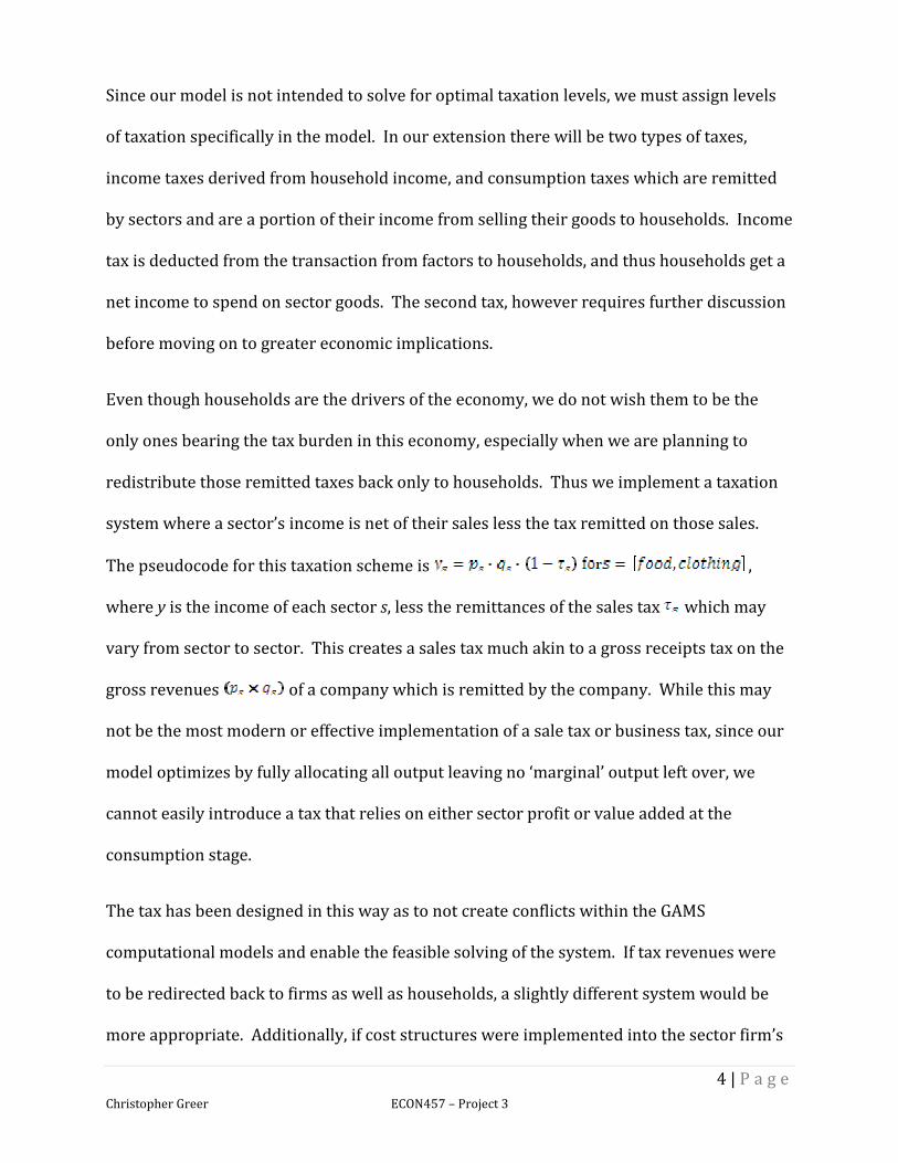
redistribute those remitted taxes back only to households. Thus we implement a taxation
system where a sector’s income is net of their sales less the tax remitted on those sales.
The pseudocode for this taxation scheme is ,
where y is the income of each sector s, less the remittances of the sales tax which may
vary from sector to sector. This creates a sales tax much akin to a gross receipts tax on the
gross revenues of a company which is remitted by the company. While this may
not be the most modern or effective implementation of a sale tax or business tax, since our
model optimizes by fully allocating all output leaving no ‘marginal’ output left over, we
cannot easily introduce a tax that relies on either sector profit or value added at the
consumption stage.
The tax has been designed in this way as to not create conflicts within the GAMS
computational models and enable the feasible solving of the system. If tax revenues were
to be redirected back to firms as well as households, a slightly different system would be
more appropriate. Additionally, if cost structures were implemented into the sector firm’s

5 | P a g e
Christopher Greer ECON457 – Project 3
output functions, then a value added tax could be created if they earn some profit in selling
their goods to households at a higher price than they buy those goods from the factors.
However, given the nature of the SAM-CGE model these systems are not very applicable
and should be left for other modelling exercises.
Redistribution of Taxation Revenue
On the redistribution side of the taxation system, we will set up a system where the
government redistributes some portion of the tax revenue back to households, who are the
only recipients of redistributed taxation revenue. The rationale behind this modelling
decision is twofold; to keep the model relatively simple, and employing the assumption that
the government transfer to households can have meanings other than a direct cash
transfer. Since we have not added government to the SAM matrix, and the purpose of
government in our model is only to tax and redistribute funds, we can make assumptions
about the meaning of those redistribution transfers without burdening the model with
additional computational or structural elements.
Most simply, we can interpret the government’s transfer of tax revenue to households as
representing income in lieu of many of the activities governments take on that citizens do
not directly purchase on the open market but are provided through programs funded by
public revenue: public safety, healthcare, maintenance of transportation and logistics
networks, environmental protection, etc. Since households do not have to pay (or in the
case of the SAM-CGE model, transfer funds) for these public goods and services out of their
income, we can assume that the increase in total income households receive from the tax
redistribution is representing the gain in ‘wealth’ or ‘utility’ from the government
providing those services as opposed to having to seek out some sector firm to provide

6 | P a g e
Christopher Greer ECON457 – Project 3
them. Since households are the recipients of all of the government transfers, they will have
additional income to spend on transfers to the sectors to purchase the commodities they
require. This in turn will drive greater demand for factor activities and further increase
relative incomes. Due to the nature of our redistribution system, we hypothesize that
households should see an increase in relative incomes even though the initial levels of
economic transfers in the economy (via the SAM) are unchanged.
Finally, we will also implement a mechanism that will allow us to vary the amount of
revenue that is actually redistributed to households. Under ideal conditions, 100% of the
revenue collected from tax remittances would be returned to households, but we can more
realistically develop a simple mechanism to allow only a portion of the government
revenue to be redistributed. If, as we are supposing, the redistribution of government
revenue to households represents the provision of public goods and services that benefit
households, then there may be some cost associated with providing those benefits. We can
then vary the level of government efficiency by making only a portion of remittances be
redistributed to households in the form of a transfer. Economically, we can also consider
the partial transfer of revenue to represent corruption within an economy where the
government retains some of its income for private purposes. We would expect that there
will be some level at which government inefficiency or corruption, as a low redistribution
percentage, will cause relative incomes in the economy to decline as households will be
made worse off by the taxation scheme. In a way, this would simulate corruption very well
as it is not unreasonable to assume that corrupt elites are not returning their graft into the
economy, but retaining it to amass private wealth or spending it outside of the economy.

7 | P a g e
Christopher Greer ECON457 – Project 3
With the theoretical basis for our model of taxation and redistribution established in the
SAM-CGE model, we now turn our attention to the description of the computational model
and the methods used to achieve the goals outlined by our theoretical model. The next
section will detail those computational changes and lead in to the section presenting our
experiments and the results of those experiments.
COMPUTATIONAL METHOD
Working from the basis of Kendrick et al’s presentation of the SAM-CGE, model we continue
to use GAMS for its strong ability to solve complex non-linear programming problems and
apply that to our SAM-CGE model with endogenous taxation. The base model uses NLP
optimization to find the best allocations of prices and quantities of goods in the economy
and incomes of the various elements of the economy. Introducing our taxation scheme
merely affects the conditions of how the model is solved, not the solution method or what
the model is optimizing. Therefore, our extension to the SAM-CGE model only requires the
addition of variables and equations related to the taxation and redistribution scheme, as
well as modifying existing equations to ensure that incomes for households and sectors are
properly adjusted.
A full print-out of the GAMS code is included in Appendix A and will be referred to in this
section and the following section of experiments and results. We also assume that readers
of this report are familiar with the language of GAMS and the basics of the SAM-CGE
mechanics in GAMS. This will prevent unnecessary duplication of background information
in the presentation of our computational modifications.
Exogenous Variables
8 | P a g e
Christopher Greer ECON457 – Project 3
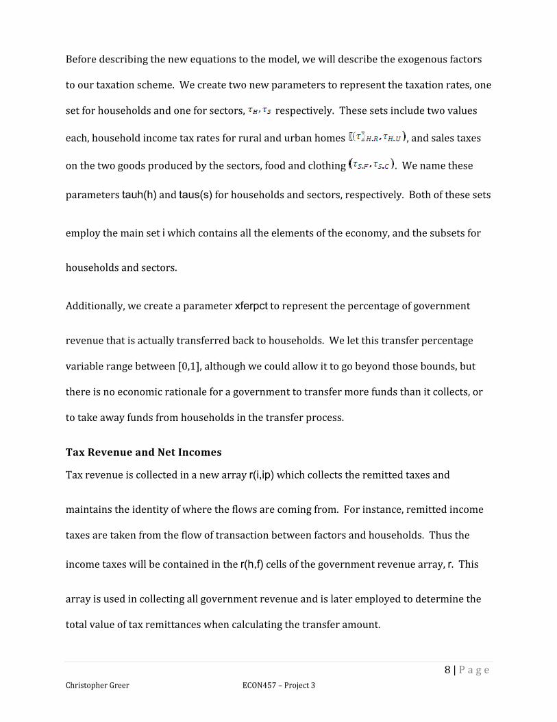
Before describing the new equations to the model, we will describe the exogenous factors
to our taxation scheme. We create two new parameters to represent the taxation rates, one
set for households and one for sectors, respectively. These sets include two values
each, household income tax rates for rural and urban homes , and sales taxes
on the two goods produced by the sectors, food and clothing . We name these
parameters tauh(h) and taus(s) for households and sectors, respectively. Both of these sets
employ the main set i which contains all the elements of the economy, and the subsets for
households and sectors.
Additionally, we create a parameter xferpct to represent the percentage of government
revenue that is actually transferred back to households. We let this transfer percentage
variable range between [0,1], although we could allow it to go beyond those bounds, but
there is no economic rationale for a government to transfer more funds than it collects, or
to take away funds from households in the transfer process.
Tax Revenue and Net Incomes
Tax revenue is collected in a new array r(i,ip) which collects the remitted taxes and
maintains the identity of where the flows are coming from. For instance, remitted income
taxes are taken from the flow of transaction between factors and households. Thus the
income taxes will be contained in the r(h,f) cells of the government revenue array, r. This
array is used in collecting all government revenue and is later employed to determine the
total value of tax remittances when calculating the transfer amount.

9 | P a g e
Christopher Greer ECON457 – Project 3
As was previously mentioned in the economic model section, we deduct two types of taxes,
an income tax on households and a sales tax on sector sales. Employing a method used by
Karadag and Westaway for income taxes, “household groups in the economy pay income
tax which is deemed to be imposed on gross income at source.” (1999, 12) In our SAM-CGE
model, households derive income from the transfer transaction from factors to households,
t(h,f). We need to deduct income taxes before they become household income, y(h), in the
set of CGE equations otherwise the NLP optimization algorithm will not solve correctly.
Before proceeding further, it is important to note that the equations that are of most import
to our extension of the model, household and sector incomes, have two sides with different
conditions to facilitate the NLP optimization. In the base case, household income, y(h), is
determined by two equations: y(h)=t(h,f) and y(h)=q(h) * p(h). These two equations
indicate that household income is determined by the transfer of funds from factors to
households (income) and that household income must also be equal to the amount value of
all goods purchased by households. Both of these conditions must be satisfied in the
solving of the NLP algorithm, and we can use these dual conditions to our advantage in
developing the taxation and redistribution extension to the base SAM-CGE model.
Returning to income taxes, we employ the r array to store the remitted taxes and introduce
the new equation erevh(h,f).. r(h,f) =E= tauh(h) * t(h,f). This equation, on line 109 of
Appendix A, takes the taxable portion of the transfer from factors to households and stores
it in the remittance array r. Secondly, we must adjust net household income. To do so we
re-write the base equation for household income on line 145 as:

10 | P a g e
Christopher Greer ECON457 – Project 3
eeyh(h).. y(h) =E= sum(f, t(h,f) * (1-tauh(h))). We remove the taxable portion of the
factor-household transfer, which is remitted to the government revenue array above, and
allow that to be the new net-of-taxation household income. This equation for household
income is now complementary to the other condition for household income, that it must
equal the purchases of households. Note that we have not modified t(h,f) in any way so the
gross flow of the factor-household transfer is left unaffected, only the resulting income
households have to spend on sector goods has been affected.
Sector sales taxes are calculated in a very similar way, with the new equation for the gross
receipts tax introduced on line 112: erevs(s,h).. r(h,s) =E= p(s) * q(h) * taus(s). Some
experimentation with the coding was required to properly nail down this equation with
respect to the use of household quantity in the equation for a sector sales tax. However,
since this is a closed economy with no savings, inventories, or investment, all products
produced by sectors must be sold to households. Therefore, the contents of the array q(h)
contain the values for household purchases of goods, which necessarily are also the amount
produced by sectors. In any event, if this model were to introduce inventories or
investment, the equation would still stand since we wish to tax only what has been sold, not
all that has been produced if some are left unsold. Additionally, the inclusion of q(h) allows
us to retain the dimensionality of the government revenue array and track which sector to
which household these sales taxes are coming from.

11 | P a g e
Christopher Greer ECON457 – Project 3
Calculating net sector income is a simpler affair and we adjust the existing equation on line
101 for sector income to eys(s).. y(s) =E= p(s) * q(s) * (1-taus(s)). This equation is the
complement to the linkage equation on line 137 of Appendix A where sector income is the
sum of transfers from households to sectors, which are purchases of food and clothing.
Since we wish to tax the gross revenue of the sectors, not the transfer of funds to sectors
from households, we have left the base linkage equation for sector income unchanged since
making the change to net income there would not allow for the correct economic
interpretation of the taxation scheme.
Government Transfers
With tax revenues and net incomes taken care of, we turn now to the transfer of
government income back to households. To do so we create two new equations to
determine the total amount of government income and then the amount of government
income that we wish to redistribute back to households. We introduce a new equation on
line 147 of Appendix A, eegy.. gy =E= sum((h,f),r(h,f)) + sum((s,h),r(s,h)). The previously
defined variable gy, representing total government income, is the sum of the contents of
the remittance array over households and sectors. This equation merely sums up the
contents of the remittance array so we get the total value of remitted taxes in a single, non-
indexed variable.
A second new equation is created that determines the amount of total government revenue
that is actually transferred back to households. This equation, on line 115 of the code
employs the xferpct variable which we exogenously set to be whatever level of government

12 | P a g e
Christopher Greer ECON457 – Project 3
effectiveness we desire in our model. The actual amount of funds transferred to
governments to households, held in the variable xfergh, is given by
etrans.. xfergh =E= gy * xferpct. We employ a non-indexed variable to hold these
amounts since in this simple model we do not need to separate transfers between
household types, nor do we need to split up transfers to different elements of the economy.
Were that the case, these transfer equations would need to be modified to accomplish that
more complex task.
Finally, to add this transfer amount to household income we return again to the equation
for household net income on line 145 and add the transfer amount back into household
income. This gives us the final version of the net household income equation given in
Appendix A, eeyh(h).. y(h) =E= sum(f, t(h,f) * (1-tauh(h))) +xfergh. Since our model is
employing NLP optimization which solves all equations simultaneously, we can both
deduct taxes and add transfers back into the same equation with no ill computational
effects. This has prevented the need to create separate equations or arrays for income and
household wealth to solve for deducting taxes and adding back transfers if we were solving
this using a non-simultaneous method.
The last computational change made to the model was with respect to Walrus’ law and
dropping one conditional equation from the NLP system. In the base model, the linkage
equation for household income was modified to only reflect rural income. Since household
income is a deterministic portion of our model, we adjusted the linkage equation for factors
to only included capital. This allows for feasible solutions from the NLP optimizer. Since

13 | P a g e
Christopher Greer ECON457 – Project 3
households are of most interest in our experiments, we will retain the base mode’s use of
urban ‘price’ as the numeraire, which will follow through in all the experiments.
EXPERIMENTS AND RESULTS
Now that the model has been fully explained, we will introduce the set of experiments and
their results. The experiments that are presented are largely stylized representations of
taxation and redistribution schemes, both using reasonable, real-world approximations,
and extreme cases to prove an economic point. We will start by presenting the base case,
without any taxation scheme as a basis for comparison against our experiments. Since we
are not modifying the initial conditions of the model with respect to the SAM, technical
coefficients, or other exogenous variables, we can make direct comparisons between our
experimental model and the base case. Full sets of results in tabular format are available in
Appendix B and will be referenced throughout the following sections.
Base Case
To calculate the base case, we used the original SAM-CGE model presented in Chapter 8 of
Kendrick et al and run the program without any modifications. For the purpose of our
experiments, we are most interested in the REPORT output giving us values of relative
prices, quantities, and incomes for each of the elements of the economy, which are
displayed in Table 1 below.
TABLE 1 - BASE CASE WITHOUT TAXATION
Price Quantity Income
Labour 0.49 2 0.979
Capital 0.673 1 0.673
Rural 1 0.735 0.735
Urban 1.013 0.906 0.918
Food 0.909 0.842 0.765

14 | P a g e
Christopher Greer ECON457 – Project 3
Clothing 1.101 0.806 0.888
With rural prices being the numeraire urban incomes are greater than rural household
incomes, a trend we will see throughout the experiments. Over the course of the
experiments we will refer back to this table and these results, especially with respect to
household incomes.
Experiment 1: Government Efficiency
Before exploring experiments involving different taxation levels, we present an experiment
focusing on the economic impact of our government efficiency variables, xferpct. For this
first experiment using our extended taxation and redistribution model, we have
implemented a set of relatively reasonable, but perhaps slightly exaggerated compared to
Canadian norms, tax rates for household incomes and the gross receipts tax. We have set
the rural income tax rate to 20% and the urban tax rate to 30%. From the SAM we know
that urban income is greater than that of rural households and, without delving into
demographic assumptions, we can also assume that urban dwellers represent a wealthier
subset of households and thus are levied higher income taxes. On the sector side, we
introduce a 15% sales tax on sector transfers to households. This value may be rather high
for a sales tax in a real world sense, but our objective here is not to model a real economy
but to derive some theoretical inferences from the changes to the economy when we
introduce our taxation and redistribution system.
The four experiments, a through d, allow the variable xferpct to vary from 100% efficiency,
meaning all of the tax revenue is redirected to households to increase their effective
income, down to 20% where the government keeps or uses 4/5ths of its revenue to facilitate
15 | P a g e
Christopher Greer ECON457 – Project 3
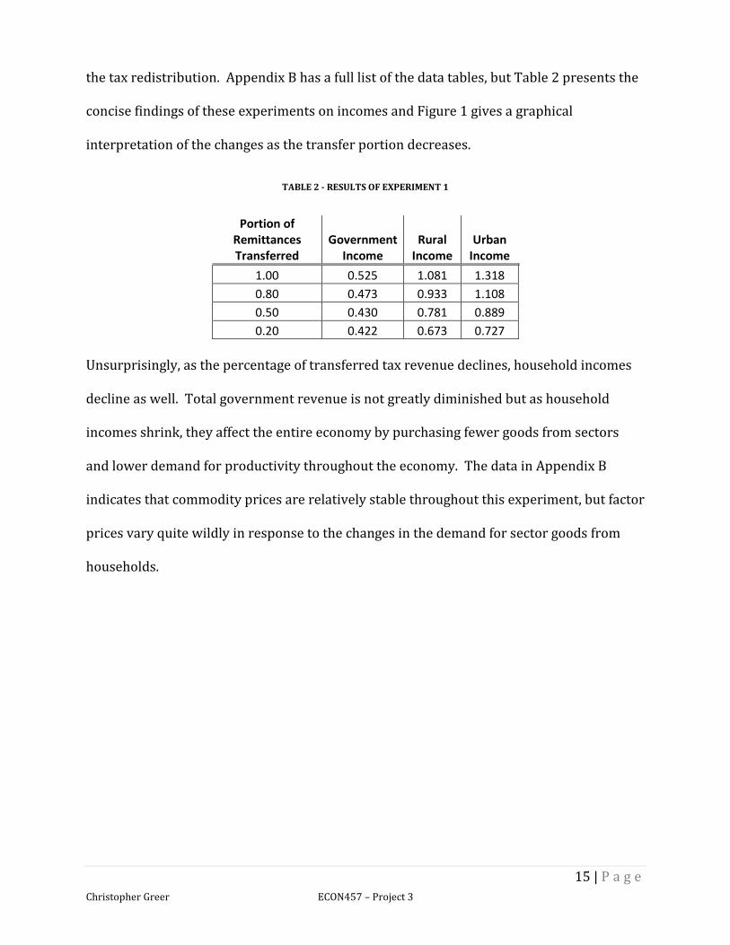
the tax redistribution. Appendix B has a full list of the data tables, but Table 2 presents the
concise findings of these experiments on incomes and Figure 1 gives a graphical
interpretation of the changes as the transfer portion decreases.
TABLE 2 - RESULTS OF EXPERIMENT 1
Portion of
Remittances
Transferred
Government
Income
Rural
Income
Urban
Income
1.00 0.525 1.081 1.318
0.80 0.473 0.933 1.108
0.50 0.430 0.781 0.889
0.20 0.422 0.673 0.727
Unsurprisingly, as the percentage of transferred tax revenue declines, household incomes
decline as well. Total government revenue is not greatly diminished but as household
incomes shrink, they affect the entire economy by purchasing fewer goods from sectors
and lower demand for productivity throughout the economy. The data in Appendix B
indicates that commodity prices are relatively stable throughout this experiment, but factor
prices vary quite wildly in response to the changes in the demand for sector goods from
households.

16 | P a g e
Christopher Greer ECON457 – Project 3
FIGURE 1 - RESULTS OF EXPERIMENT 1 VARYING GOVERNMENT EFFECTIVENESS, XFERPCT
Figure 1 details the decline of relative incomes in the economy as government effectiveness
falls. Interestingly, it is not until the transfer percentage drops down to around 50% that
we see a decline in one of the household groups relative incomes compared to the base case
without taxation. At 20% government effectiveness, both household groups are well below
their base case incomes.
From this experiment we can draw the conclusions that as the percentage of tax revenue
funds transferred to households decreases, relative incomes of households also shrink
along with the reduction of incomes in the economy as a whole. Additionally, we can
establish that we can bring down the government effectiveness by smaller amounts and not

17 | P a g e
Christopher Greer ECON457 – Project 3
negatively affect the economy. This finding will carry forward into our next experiments
where we introduce a slightly realistic assumption that not all tax revenue is spent on
transfers to households. Since we can bring the xferpct value down below 1.0 without
reducing household incomes below their original level, we can carry that assumption of
non-perfect transfer to the next set of experiments.
Experiment 2: Varying Rural Tax Levels
In this experiment, and our further experiments, we fix the percentage of tax revenue
transferred to households at 80%. For the four iterations in this experiment we let rural
taxes vary from nothing up to 50% of their income. The results of this experiment are
displayed in Table 3 and depicted in Figure 2.
TABLE 3- RESULTS OF EXPERIMENT 2, VARYING RURAL TAX RATES
Rural
Taxes
Government
Income
Rural
Income
Urban
Income
0.00 0.318 0.950 0.964
0.05 0.356 0.945 0.999
0.30 0.552 0.926 1.183
0.50 0.715 0.919 1.340
At low levels of taxation, both rural and urban households see an increase over their base
incomes but rural households see the largest gains, unsurprisingly. Rather counter-
intuitively, as rural tax rates climb urban households see strong gains in their relative
incomes and at even 50% of their income being taxed rural households see only a very
small decline in their relative income.

18 | P a g e
Christopher Greer ECON457 – Project 3
FIGURE 2- RESULTS OF EXPERIMENT 2
Figure 2 shows how the income gap between rural and urban households grows as rural
taxes climb. Government revenue also sees a strong growth as income taxes rise and its
increased levying of taxes do not appear to be negative drags on the economy – though that
is likely largely due to the way we have structured our redistribution system. Presumably,
urban households are the main beneficiaries of the increased taxation of rural households
since both household subsets share the government transfer equally, not in proportion to
their tax burden.
Without presenting data here, we ran additional simulations where we let the urban tax
rate vary and observed similar results to experiment 2 except that rural households now
19 | P a g e
Christopher Greer ECON457 – Project 3
saw increases to their relative incomes. At low tax rates the income differential is low, but
as the tax rates become higher, the household with the lower tax rate seems to benefit
more. With some trial-and-error experimentation, we found that a rural tax rate of 10%
and an urban tax rate of 40% created nearly equal relative incomes (1.035 and 1.043 for
rural and urban, respectively).
We suspect that this phenomenon is due to the setup of transaction transfers in the SAM.
Urban households are presented as having greater purchasing power in the economy, as
their sum of flows to sectors are 150 units, while rural households only provide 120 units
worth of transfers. Since urban households are ‘wealthier’ they are more capable of
handling the higher tax burden and when receiving equal amounts of government transfers
their relative income increases by a greater amount. It would appear that in this economy,
due to the wealth ‘endowment’ to urban households in the SAM, urban households will
largely be the beneficiaries of any income taxation scheme.
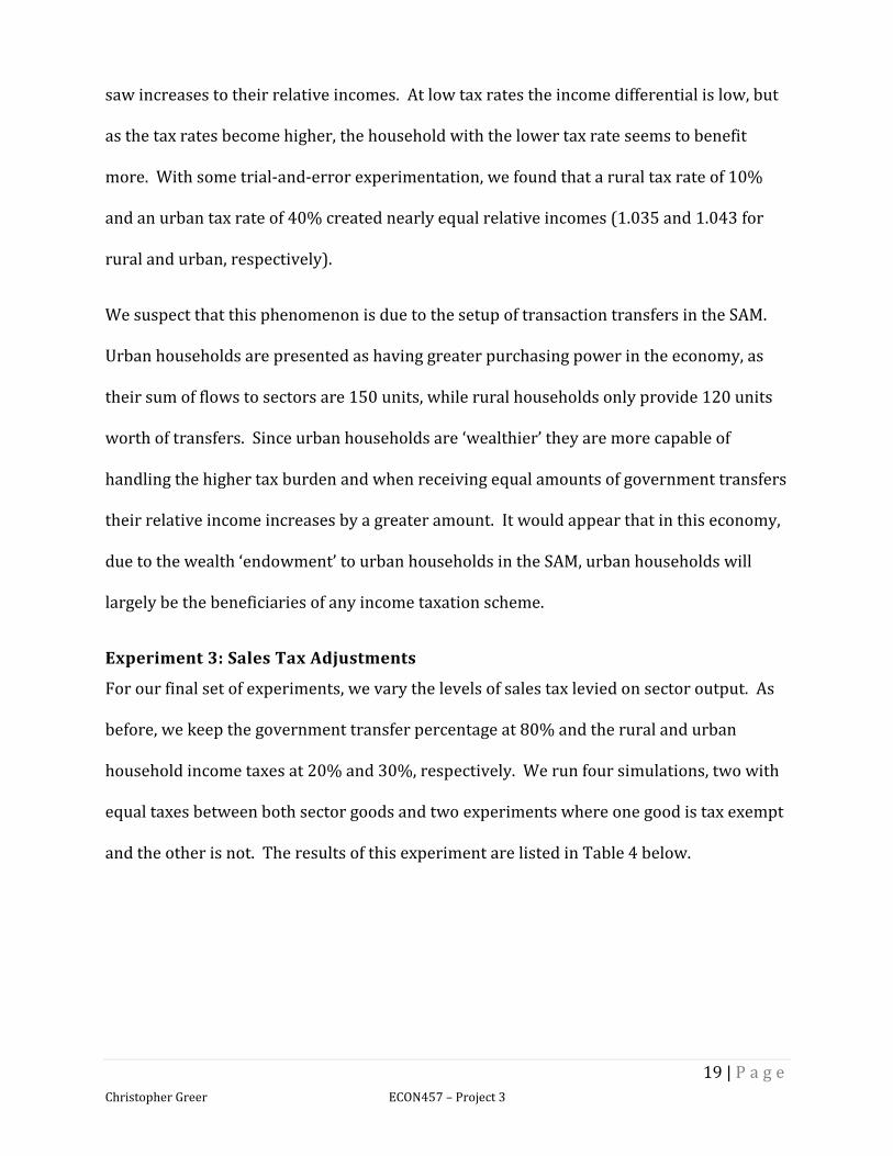
Experiment 3: Sales Tax Adjustments
For our final set of experiments, we vary the levels of sales tax levied on sector output. As
before, we keep the government transfer percentage at 80% and the rural and urban
household income taxes at 20% and 30%, respectively. We run four simulations, two with
equal taxes between both sector goods and two experiments where one good is tax exempt
and the other is not. The results of this experiment are listed in Table 4 below.

20 | P a g e
Christopher Greer ECON457 – Project 3
TABLE 4 - RESULTS OF EXPERIMENT 3, VARYING SALES TAXES
Food Tax 0.05 0.30 0.15 0.00
Clothing Tax 0.05 0.30 0.00 0.15
Government Income 0.443 0.814 0.436 0.438
Rural Income 0.909 1.256 0.909 0.910
Urban Income 1.029 1.679 1.040 1.046
Food Sector Income 0.901 1.356 0.905 0.908
Clothing Sector
Income 1.038 1.580 1.044 1.047
As we can see, when taxes are uniformly increased there is an increase in incomes both in
households and in the sectors. This result seems counterintuitive for sectors, as the sales
tax is being deducted from their income, but it would appear that the additional income
given to households more than offsets the loss to sectors from tax remittances. However,
the across the board increases in household income, particularly under the high sales tax
scenario shows that collecting taxes from businesses and returning them to households to
help stimulate purchasing does work, and strikingly so.
In the full tables of results in Appendix B we see that quantities produced when one
commodity is tax exempt do not change much. Since the sales tax is levied on sectors, not
households, it will not affect household purchasing decisions to substitute away from one
good to another. Sectors determine their production levels by the transaction flows in the
SAM and the prices of those goods, not through a typical production function which
prevents the substitution away from taxed goods to exempt goods. Sector incomes are
largely unaffected by the exemption of one product from taxation and remain quite close to
incomes seen in the 15% sales tax simulation for both goods given the same income taxes
and government efficiency. Similarly, rural and urban incomes are not strongly influenced

21 | P a g e
Christopher Greer ECON457 – Project 3
by the tax exempt status of either good since they do not have to pay that tax and their
transfers to each sector are determined by the SAM, not through consumer theory
optimization.
DISCUSSION
Throughout all of our experiments there has been one overarching theme, taxation of
incomes and a gross receipts tax, redistributed to households to increase their purchasing
power and effective incomes, provides significant gains in an economy. Since the SAM-CGE
model takes the flows of transactions as given and then determines prices and quantities
produced by the sectors (and through that mechanism, incomes) our taxation system
should not be introducing any new income into the economy, only redistributing the flows
in a way that simultaneously affects prices and quantities. Our discussion will reflect on
how the findings from our experiments take the given transactions scheme of the SAM and
determine what influence we can infer from our implemented taxation and redistribution
scheme, especially on our key indicator – household incomes.
Much like the constant theme of our taxation scheme generating greater relative incomes
for households in the economy, we have seen how important households are as the drivers
of our simulated economy. When our redistributive scheme increases net household
incomes, sectors and factors benefit as well due to the conditions in the model imposed by
Walrus’ law. Since there can be no savings, and interior solutions found by the NLP
optimizer must meet the conditions where all income of each element of the economy is
spent on its required good, a benefit to one element of the economy passes through to all
the other elements. We could prove this in another way by increasing the transfers from
factors to households in the SAM and we would see an increase in incomes throughout the

22 | P a g e
Christopher Greer ECON457 – Project 3
economy. But our experiments have shown that redistributing more tax revenue to
households provides a significant benefit in incomes for both sectors and factors.
Taking these simulation findings and applying them to a real economy does pose certain
problems. First and foremost, our model redistributes government revenue in a very
stylized way. In our economic model section we have made the supposition that transfers
to households imply the value of public goods and services that governments provide
which would cost much more to individual households had they to purchase those services
on the open market. However, it may be that this assumption has led to the development of
a computational method that overstates the increase in household incomes through these
redistributive efforts. This would lead to a cascading effect in the SAM-CGE optimization of
prices and quantities of the elements of the economy which may explain the exceptional
relative increases in household income we have seen in our experiments. But, if we view
these changes in relative incomes more as welfare gains, then the results may not be that
misleading if we draw parallels to a real economy. This supposition leads to a problem of
taking too many assumptions or stylizations about our model since the SAM-CGE format
explicitly measures flows of transactions between the elements in an economy. With all
these considerations in mind we should take the magnitude of the findings in our model
with a grain of salt but not lose sight of the possibility that, under this simulation, a scheme
of taxation and redistribution directly to households really does have an expanding effect
on the economy.
While reviewing the findings from the experiment, one economic phase came to mind:
“Reaganomics.” The idea of direct transfers to households as a stylized form of trickle-
down-economics seems to be a plausible way of interpreting the assumptions we have

23 | P a g e
Christopher Greer ECON457 – Project 3
made about the redistribution scheme and our findings. However, perhaps reverse-
Reaganomics would be a better phrase, since our simulations seem to indicate that raising
taxes actually has a very strong growth effect to incomes, particularly household incomes,
in our small closed economy. However, when looking at relative tax rates, experiment 2
seems to indicate that higher relative tax rates on the less wealthy (rural households in our
model) does have a significant benefit on urban households but also produces a relative
gain in household incomes across the board. While it is not my personal view to espouse
such trickle-down taxation policies as a matter of public finance policy, our simulations of a
small closed economy do seem to indicate that it might just work.
Another aspect of our findings that we can relate to economic theory is how our household
incomes, and incomes throughout the economy, do not appear to have hit the apex of the
Laffer curve yet. In all our simulations, increasing the taxation rate, assuming a constant
rate of government transfers to households, has led to increased incomes and outputs in
the economy. This would suggest that our simulations had not reached taxation levels that
hit the downward sloping side of the Laffer curve, where excessive taxation has caused the
economy to shrink. While the Laffer curve is often associated with supply-side economics
and other macroeconomics and taxation policy discussions related to reducing the taxation
and regulation burdens on suppliers to produce economic stimuli, it should be noted that
our simulations have shown that high levels of supply-side taxation also lead to significant
gains in household and sector incomes. Again, due to the simplistic nature of our model
and the way in which taxes are redistributed in the economy, it is difficult to use our
findings to prove a theory or apply directly to a real-world situation. Nevertheless, if we
accept the Laffer curve as a valid method of assessing taxation policy, it would seem that

24 | P a g e
Christopher Greer ECON457 – Project 3
our model and simulations have been successful in producing benefits and we have yet to
simulate a situation where we are on the downward sloping side of the Laffer curve.
Finally, a note on our first experiment regarding the percentage of government funds
transferred to households. Using this as a measure of government efficiency or corruption,
the results from our experiment showed how strongly an effect low levels of efficiency can
have on households incomes and incomes in the economy as a whole. Our simulations
showed how low levels of taxation redistribution can harm the growth in an economy that
was intended through redistributing tax revenue to the economic drivers, homes. This also
sheds some light on how problems of corruption can seriously affect the growth of an
economy and artificially depress prices and incomes. While we do not simulate the effects
of trade, or pay significant attention to prices and inflation in our simulations, we can still
infer that when governments are inefficient or corrupt and do not redistribute those tax
levies, the economy seriously suffers.
CONCLUSION
In this paper we have presented a series of experiments dealing with the introduction of a
simplified taxation and redistribution scheme in a closed economy using a SAM-CGE model.
By levying taxes on household income and sales taxes on sector output, then redistributing
that government revenue back to households, our simulations have demonstrated relative
growth is possible within the confines of our simplified economy. Using household income
levels as our key metric, we have seen that increasing tax levels have also lead to increased
incomes, prices, and activity in the economy given the exogenously given levels of fund
transactions in the social accounting matrix.

25 | P a g e
Christopher Greer ECON457 – Project 3
However, we should use caution in taking the results from our simulations and applying
them to economic theories or real policy discourses. Our computational model remains
very simplistic and our taxation and redistribution system is based on a number of
assumptions about the meaning of those government transfers. Because of those
assumptions, and the somewhat surprising results of our simulations, the magnitudes of
our findings should not be explicitly relied on, but we should look more at the relative
effect on the different elements of the economy, most especially households. Nevertheless,
this simulation has given us some insight into how significant some small structural
changes to a SAM-CGE model can be and how interlinked the elements of a closed economy
are when presented in this form.

26 | P a g e
Christopher Greer ECON457 – Project 3
BIBLIOGRAPHY
Karadag, Metin, and Tony Westaway. A SAM-Based Computable General Equilibrium Model
of the Turkish Economy. Economic Research Paper No. 99/18, Loughborough UK:
Loughborough University, 1999.
Kendrick, David A., P. Reuben Mercado, and Hans M. Amman. Computational Economics.
Princeton: Princeton University Press, 2006.

0 | A p p e n d i x A
Christopher Greer ECON457 – Project 3
$TITLE SAM-Taxation 1 * APPENDIX A - SAM-CGE MODEL WITH TAXATION 2 * Developed by Ruben Mercado 3 * Modified by Alan Mehlenbacher 4 5 * Extended by Christopher Greer - 6 * ECON457 Winter 2012 7 8 options limrow = 4; 9 option NLP=MINOS; 10 11 SETS 12 i general index /labor, capital, rural, urban, food, clothing/ 13 s(i) sectors /food, clothing/ 14 f(i) factors /labor, capital/ 15 h(i) households /rural, urban/ 16 ALIAS (i,ip); 17 ALIAS (i,iq); 18 19 PARAMETERS 20 b(s) technical coefficients 21 a(i,ip) share coefficients 22 tauh(h) household taxes 23 taus(s) sector taxes 24 xferpct percentage of govt revenue transfered ; 25 b('food') = 1.2; b('clothing') = 1.0; 26 27 *Income tax rates for rural and urban households 28 tauh('rural') = 0.2; tauh('urban') = 0.3; 29 *Sales tax on sector-produced goods 30 taus(s) = 0.15; 31 *taus('clothing') = 0.30; taus('food') = 0.30; 32 *Precentage of government tax revenue transfered 33 xferpct = 0.8; 34 35 36 37
1 | A p p e n d i x A
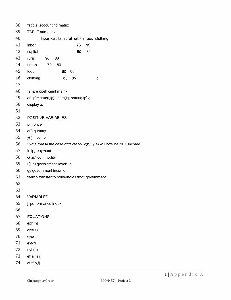
Christopher Greer ECON457 – Project 3
*social accounting matrix 38 TABLE sam(i,ip) 39 labor capital rural urban food clothing 40 labor 75 85 41 capital 50 60 42 rural 90 30 43 urban 70 80 44 food 60 65 45 clothing 60 85 ; 46 47 *share coefficient matrix 48 a(i,ip)= sam(i,ip) / sum(iq, sam(iq,ip)); 49 display a; 50 51 POSITIVE VARIABLES 52 p(i) price 53 q(i) quantiy 54 y(i) income 55 *Note that in the case of taxation, y(h), y(s) will now be NET income 56 t(i,ip) payment 57 c(i,ip) commodity 58 r(i,ip) government revenue 59 gy government income 60 xfergh transfer to households from government 61 62 63 VARIABLES 64 j performance index; 65 66 EQUATIONS 67 eph(h) 68 eqs(s) 69 eys(s) 70 eyf(f) 71 eyh(h) 72 etfs(f,s) 73 ethf(h,f) 74

2 | A p p e n d i x A
Christopher Greer ECON457 – Project 3
etsh(s,h) 75 eetsh(s,h) 76 ecfs(f,s) 77 eeys(s) 78 eeyf(f) 79 eeyh(h) 80 *Taxation 81 erevh(h,f) 82 erevs(s,h) 83 *Redistribution 84 etrans 85 *Market clearing of taxes 86 eegy Total government income 87 88 jd performance index definition; 89 * performance index equation 90 jd.. j =E= 0; 91 92 *SECTORS 93 *Output sector quantity (product of the commmodity^(share coeff)) 94 eqs(s).. q(s) =E= b(s)* prod(f, c(f,s)**a(f,s)); 95 *Input sector quantity (commodity over factor and sector, product of 96 *sector p*q div the price for that sector 97 *Commodity flow from factors to sectors 98 ecfs(f,s).. c(f,s) =E= a(f,s) * q(s) * p(s) / p(f); 99 *Net Income for sectors output less consumption taxes 100 eys(s).. y(s) =E= p(s) * q(s) * (1-taus(s)); 101 *Payments from sectors to factors, business purchases? 102 *(factor price times that commodity for a given sector) 103 etfs(f,s).. t(f,s) =E= p(f) * c(f,s); 104 105 106 *GOVERNMENT REVENUE 107 *Household taxes, summed over households (income tax) 108 erevh(h,f).. r(h,f) =E= tauh(h) * t(h,f); 109 *Taxes on sector production summed over sectors 110 *Consumption tax on each unit of food/clothing consumed 111

3 | A p p e n d i x A
Christopher Greer ECON457 – Project 3
erevs(s,h).. r(h,s) =E= p(s) * q(h) * taus(s); 112 113 *GOVERNMENT TRANSFERS AMOUNT 114 etrans.. xfergh =E= gy * xferpct; 115 116 *FACTORS 117 *Factor price-quantity (income) 118 eyf(f).. y(f) =E= p(f) * q(f); 119 *Payments from factors to households (wages) - deduct income taxes here 120 ethf(h,f).. t(h,f) =E= a(h,f) * y(f); 121 122 *HOUSEHOLDS 123 *Purchases by households to sectors as a function of household income 124 *since households spend all their income on sector goods 125 etsh(s,h).. t(s,h) =E= a(s,h) * y(h); 126 *CPI 127 eph(h).. p(h) =E= prod(s, p(s)**a(s,h)); 128 *Flow of money from sectors to households (from purchases) 129 eetsh(s,h).. t(s,h) =E= p(s) * c(s,h); 130 *Household purchases cannot exceed income 131 eyh(h).. y(h) =E= p(h) * q(h); 132 133 134 *LINKAGES 135 *Sector NET income (sales) less consumption taxes 136 eeys(s).. y(s) =E= sum(h, t(s,h)); 137 *Factor income as sum of payments from sectors to factors, over sectors 138 *Eliminating one of the factors to satisfy Walrus' law for feasibility 139 eeyf('capital').. y('capital') =E= sum(s,t('capital',s)); 140 141 *Household NET income PLUS transfers from government 142 *Gov't transfer added here since household income plays a part in determining 143 *sector purchases 144 eeyh(h).. y(h) =E= (sum(f, t(h,f) * (1-tauh(h)))) + xfergh; 145 *Total government revenue 146 eegy.. gy =E= sum((h,f),r(h,f)) + sum((s,h),r(s,h)); 147 148

4 | A p p e n d i x A
Christopher Greer ECON457 – Project 3
149 *initial values to facilitate solver convergence 150 p.l(i) = 1; q.l(i) = 1; y.l(i) = 1; 151 152 *lower bound to avoid division by zero 153 p.lo(f) = 0.001; 154 155 *lower bounds to avoid undefined derivatives in exponential functions 156 p.lo(s) = 0.001; c.lo(f,s) = 0.001; 157 158 *exogenous variables 159 q.fx('labor') = 2; q.fx('capital') = 1; 160 161 *numeraire 162 p.fx('rural') = 1; 163 164 MODEL SAMDK_TAX /all/; 165 option iterlim = 10000; 166 SOLVE SAMDK_TAX MAXIMIZING J USING NLP; 167 168 PARAMETER REPORT; 169 REPORT(i, "price") = p.l(i); 170 REPORT(i, "quantity") = q.l(i); 171 REPORT(i, "income") = y.l(i); 172 173 DISPLAY REPORT; DISPLAY gy.l, r.l; 174
175
5 | A p p e n d i x B
Christopher Greer ECON457 – Project 3
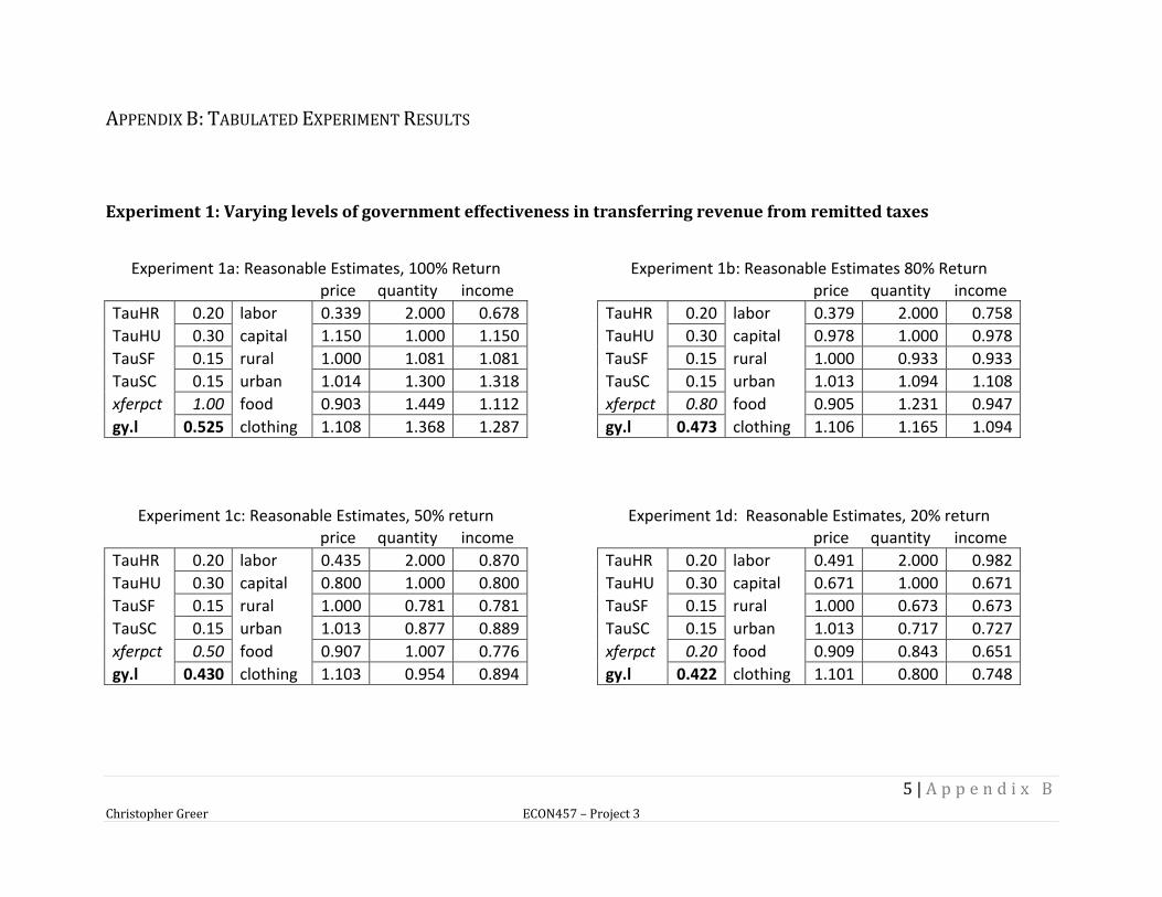
APPENDIX B: TABULATED EXPERIMENT RESULTS
Experiment 1: Varying levels of government effectiveness in transferring revenue from remitted taxes
Experiment 1a: Reasonable Estimates, 100% Return Experiment 1b: Reasonable Estimates 80% Return
price quantity income price quantity income
TauHR 0.20 labor 0.339 2.000 0.678 TauHR 0.20 labor 0.379 2.000 0.758
TauHU 0.30 capital 1.150 1.000 1.150 TauHU 0.30 capital 0.978 1.000 0.978
TauSF 0.15 rural 1.000 1.081 1.081 TauSF 0.15 rural 1.000 0.933 0.933
TauSC 0.15 urban 1.014 1.300 1.318 TauSC 0.15 urban 1.013 1.094 1.108
xferpct 1.00 food 0.903 1.449 1.112 xferpct 0.80 food 0.905 1.231 0.947
gy.l 0.525 clothing 1.108 1.368 1.287 gy.l 0.473 clothing 1.106 1.165 1.094
Experiment 1c: Reasonable Estimates, 50% return Experiment 1d: Reasonable Estimates, 20% return
price quantity income price quantity income
TauHR 0.20 labor 0.435 2.000 0.870 TauHR 0.20 labor 0.491 2.000 0.982
TauHU 0.30 capital 0.800 1.000 0.800 TauHU 0.30 capital 0.671 1.000 0.671
TauSF 0.15 rural 1.000 0.781 0.781 TauSF 0.15 rural 1.000 0.673 0.673
TauSC 0.15 urban 1.013 0.877 0.889 TauSC 0.15 urban 1.013 0.717 0.727
xferpct 0.50 food 0.907 1.007 0.776 xferpct 0.20 food 0.909 0.843 0.651
gy.l 0.430 clothing 1.103 0.954 0.894 gy.l 0.422 clothing 1.101 0.800 0.748

6 | A p p e n d i x B
Christopher Greer ECON457 – Project 3
Experiment 2: Varying Rural Taxes
Experiment 2a: No Rural Tax Experiment 2b: 5% Rural Tax
price quantity income price quantity income
TauHR 0.00 labor 0.396 2.000 0.792 TauHR 0.05 labor 0.392 2.000 0.784
TauHU 0.30 capital 0.917 1.000 0.917 TauHU 0.30 capital 0.932 1.000 0.932
TauSF 0.15 rural 1.000 0.950 0.950 TauSF 0.15 rural 1.000 0.945 0.945
TauSC 0.15 urban 1.013 0.951 0.964 TauSC 0.15 urban 1.013 0.986 0.999
xferpct 0.80 food 0.905 1.160 0.893 xferpct 0.80 food 0.905 1.177 0.906
gy.l 0.318 clothing 1.105 1.088 1.021 gy.l 0.356 clothing 1.105 1.106 1.039
Experiment 2c: 10% Rural Tax Experiment 2d: 50% Rural Tax
price quantity income price quantity income
TauHR 0.30 labor 0.370 2.000 0.741 TauHR 0.50 labor 0.353 2.000 0.707
TauHU 0.30 capital 1.011 1.000 1.011 TauHU 0.30 capital 1.083 1.000 1.083
TauSF 0.15 rural 1.000 0.926 0.926 TauSF 0.15 rural 1.000 0.919 0.919
TauSC 0.15 urban 1.014 1.167 1.183 TauSC 0.15 urban 1.014 1.322 1.340
xferpct 0.80 food 0.904 1.27 0.976 xferpct 0.80 food 0.903 1.354 1.040
gy.l 0.552 clothing 1.106 1.206 1.134 gy.l 0.715 clothing 1.107 1.295 1.219
7 | A p p e n d i x B
Christopher Greer ECON457 – Project 3
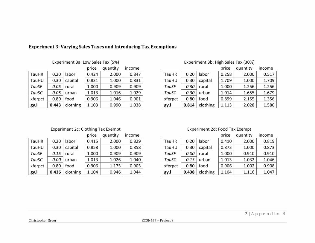
Experiment 3: Varying Sales Taxes and Introducing Tax Exemptions
Experiment 3a: Low Sales Tax (5%) Experiment 3b: High Sales Tax (30%)
price quantity income price quantity income
TauHR 0.20 labor 0.424 2.000 0.847 TauHR 0.20 labor 0.258 2.000 0.517
TauHU 0.30 capital 0.831 1.000 0.831 TauHU 0.30 capital 1.709 1.000 1.709
TauSF 0.05 rural 1.000 0.909 0.909 TauSF 0.30 rural 1.000 1.256 1.256
TauSC 0.05 urban 1.013 1.016 1.029 TauSC 0.30 urban 1.014 1.655 1.679
xferpct 0.80 food 0.906 1.046 0.901 xferpct 0.80 food 0.899 2.155 1.356
gy.l 0.443 clothing 1.103 0.990 1.038 gy.l 0.814 clothing 1.113 2.028 1.580
Experiment 2c: Clothing Tax Exempt Experiment 2d: Food Tax Exempt
price quantity income price quantity income
TauHR 0.20 labor 0.415 2.000 0.829 TauHR 0.20 labor 0.410 2.000 0.819
TauHU 0.30 capital 0.858 1.000 0.858 TauHU 0.30 capital 0.873 1.000 0.873
TauSF 0.15 rural 1.000 0.909 0.909 TauSF 0.00 rural 1.000 0.910 0.910
TauSC 0.00 urban 1.013 1.026 1.040 TauSC 0.15 urban 1.013 1.032 1.046
xferpct 0.80 food 0.906 1.175 0.905 xferpct 0.80 food 0.906 1.002 0.908
gy.l 0.436 clothing 1.104 0.946 1.044 gy.l 0.438 clothing 1.104 1.116 1.047