enee631 digital image processing (spring'04) basics on image compression spring ’04...

ENEE631 Digital Image Processing (Spring'04)

Basics on Image CompressionBasics on Image Compression

Spring ’04 Instructor: Min Wu

ECE Department, Univ. of Maryland, College Park

www.ajconline.umd.edu (select ENEE631 S’04) [email protected]

Based on ENEE631 Based on ENEE631 Spring’04Spring’04Section 8Section 8

ENEE631 Digital Image Processing (Spring'04) Lec9 – Basics on Compression [4]

Image CompressionImage Compression

Part-1. BasicsPart-1. Basics

UM

CP

EN

EE

63

1 S

lide

s (c

rea

ted

by

M.W

u ©

20

04

)


Why Need Compression?Why Need Compression?

Savings in storage and transmission

– multimedia data (esp. image and video) have large data volume– difficult to send real-time uncompressed video over current

network

Accommodate relatively slow storage devices

– they do not allow playing back uncompressed multimedia data in real time

1x CD-ROM transfer rate ~ 150 kB/s 320 x 240 x 24 fps color video bit rate ~ 5.5MB/s=> 36 seconds needed to transfer 1-sec uncompressed video

from CD

UM

CP

EN

EE

63

1 S

lide

s (c

rea

ted

by

M.W

u ©

20

01

)


Example: Storing An EncyclopediaExample: Storing An Encyclopedia

– 500,000 pages of text (2kB/page) ~ 1GB => 2:1 compress

– 3,000 color pictures (64048024bits) ~ 3GB => 15:1

– 500 maps (64048016bits=0.6MB/map) ~ 0.3GB => 10:1

– 60 minutes of stereo sound (176kB/s) ~ 0.6GB => 6:1

– 30 animations with average 2 minutes long

(64032016bits16frames/s=6.5MB/s) ~ 23.4GB => 50:1

– 50 digitized movies with average 1 minute long

(64048024bits30frames/s = 27.6MB/s) ~ 82.8GB => 50:1

Require a total of 111.1GB storage capacity if without compression Reduce to 2.96GB if with compression

From Ken Lam’s DCT talk 2001 (HK Polytech)U

MC

P E

NE

E6

31

Slid

es

(cre

ate

d b

y M

.Wu

© 2

00

1)


PCM codingPCM coding

How to encode a digital image into bits?– Sampling and perform uniform quantization

“Pulse Coded Modulation” (PCM) 8 bits per pixel ~ good for grayscale image/video 10-12 bpp ~ needed for medical images

Reduce # of bpp for reasonable quality via quantization– Quantization reduces # of possible levels to encode– Visual quantization: dithering, companding, etc.

Halftone use 1bpp but usually upsampling ~ saving less than 2:1

Encoder-Decoder pair codec

I(x,y)

Input imageSampler Quantizer Encoder

transmit

image capturing device

UM

CP

EN

EE

63

1 S

lide

s (c

rea

ted

by

M.W

u ©

20

01

)


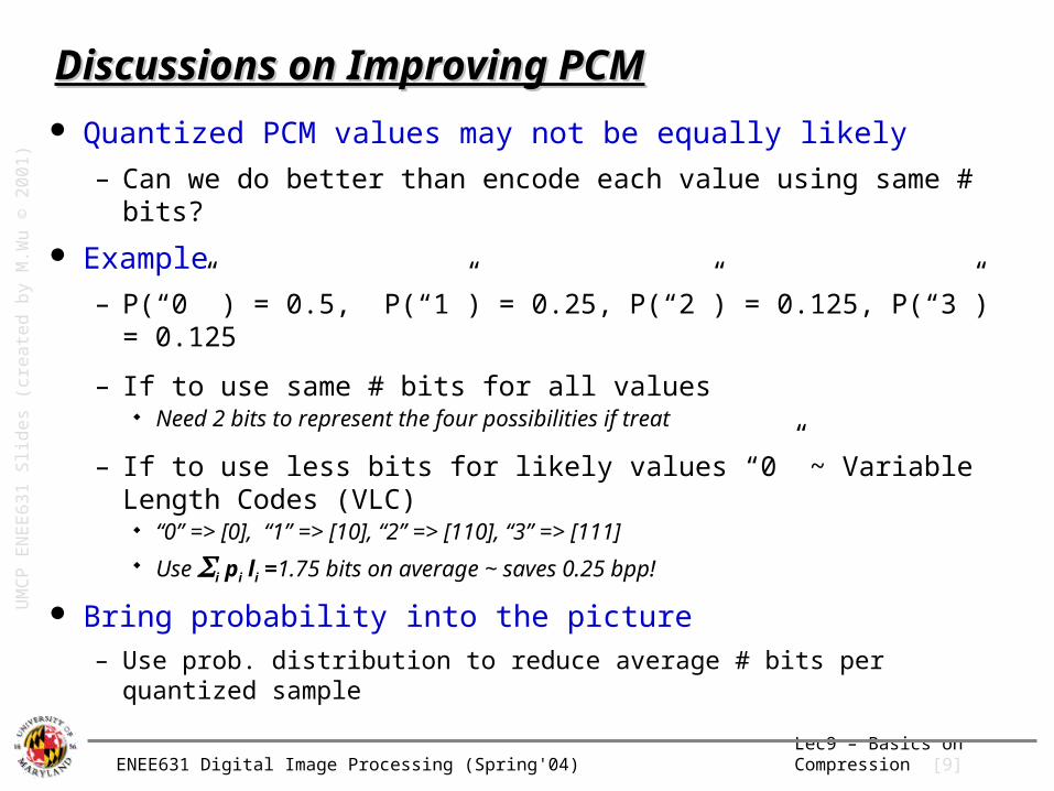
Discussions on Improving PCMDiscussions on Improving PCM

Quantized PCM values may not be equally likely

– Can we do better than encode each value using same # bits?

Example

– P(“0” ) = 0.5, P(“1”) = 0.25, P(“2”) = 0.125, P(“3”) = 0.125

– If to use same # bits for all values Need 2 bits to represent the four possibilities if treat

– If to use less bits for likely values “0” ~ Variable Length Codes (VLC)

“0” => [0], “1” => [10], “2” => [110], “3” => [111] Use i pi li =1.75 bits on average ~ saves 0.25 bpp!

Bring probability into the picture– Use prob. distribution to reduce average # bits per quantized sample

UM

CP

EN

EE

63

1 S

lide

s (c

rea

ted

by

M.W

u ©

20

01

)


Entropy CodingEntropy Coding

Idea: use fewer bits for commonly seen values

At least how many # bits needed?– Limit of compression => “Entropy”

Measures the uncertainty or avg. amount of information of a source

Definition: H = i pi log2 (1 / pi) bits e.g., entropy of previous example is 1.75

Can’t represent a source perfectly with less than avg. H bits per sample

Can represent a source perfectly with avg. H+ bits per sample ( Shannon Lossless Coding Theorem )

– “Compressability” depends on the sources

Important to design a codebook to decode coded stream efficiently and without ambiguity

See info. theory course (EE721) for more theoretical details

UM

CP

EN

EE

63

1 S

lide

s (c

rea

ted

by

M.W

u ©

20

01

/20

04

)


E.g. of Entropy Coding: Huffman CodingE.g. of Entropy Coding: Huffman Coding

Variable length code – assigning about log2 (1 / pi) bits for the ith value

has to be integer# of bits per symbol

Step-1– Arrange pi in decreasing order and consider them as tree leaves

Step-2– Merge two nodes with smallest probabilities to a new node and

sum up probabilities– Arbitrarily assign 1 and 0 to each pair of merging branch

Step-3– Repeat until no more than one node left.– Read out codeword sequentially from root to leaf

UM

CP

EN

EE

63

1 S

lide

s (c

rea

ted

by

M.W

u ©

20

01

)


Huffman Coding (cont’d)Huffman Coding (cont’d)

S0

S1

S2

S3

S4

S5

S6

S7

000

001

010

011

100

101

110

111

PCM

00

10

010

011

1100

1101

1110

1111

Huffman

(trace from root)

0.25

0.21

0.15

0.14

0.0625

0.0625

0.0625

0.06250.125

10

0.12510

0.251

0

0.2910

0.54

1

0

0.46

1

01.0

1

0

UM

CP

EN

EE

63

1 S

lide

s (c

rea

ted

by

M.W

u ©

20

01

)


Huffman Coding: Pros & ConsHuffman Coding: Pros & Cons Pro

– Simplicity in implementation (table lookup)– Given symbol size, Huffman coding gives best coding efficiency

Con

– Need to obtain source statistics– The codelength has to be integer => lead to gaps between its average

codelength and entropy

Improvement

– Code a group of symbols as a whole: allow fractional # bits/symbol– Arithmetic coding: fractional # bits/symbol

– Lempel-Ziv coding or LZW algorithm “universal”, no need to estimate source statistics fix-length codeword for variable-length source symbols

UM

CP

EN

EE

63

1 S

lide

s (c

rea

ted

by

M.W

u ©

20

01

)


Run-Length CodingRun-Length Coding

How to efficiently encode it? e.g. a row in a binary doc image:

“ 0 0 0 0 0 0 0 1 1 0 0 0 1 0 1 0 0 0 0 0 0 1 1 1 …”

Run-length coding (RLC)

– Code length of runs of “0” between successive “1” run-length of “0” ~ # of “0” between “1” good if often getting frequent large runs of “0” and sparse “1”

– E.g., => (7) (0) (3) (1) (6) (0) (0) … …

– Assign fixed-length codeword to run-length in a range (e.g. 0~7)– Or use variable-length code like Huffman to further improve

RLC also applicable to general a data sequence with many consecutive “0” (or long runs of other values)

UM

CP

EN

EE

63

1 S

lide

s (c

rea

ted

by

M.W

u ©

20

01

)


Probability Model of Run-Length CodingProbability Model of Run-Length Coding Assume “0” occurs independently w.p. p: (p is close to 1)

Prob. of getting an L runs of “0”: possible runs L=0,1, …, M

– P( L = l ) = pL (1-p) for 0 l M-1 (geometric distribution)– P( L = M ) = pM (when having M or more “0”)

Avg. # binary symbols per zero-run

– Savg = L (L+1) pL (1-p) + M pM = (1 – pM ) / ( 1 – p )

Compression ratio

C = Savg / log2 (M+1) = (1 – pM ) / [( 1–p ) log2(M+1)]

Example

– p = 0.9, M=15 Savg = 7.94, C = 1.985, H = 0.469 bpp

– Avg. run-length coding rate Bavg = 4 bit / 7.94 ~ 0.516 bpp

– Coding efficiency = H / Bavg ~ 91%

UM

CP

EN

EE

63

1 S

lide

s (c

rea

ted

by

M.W

u ©

20

01

)


QuantizationQuantization

UM

CP

EN

EE

63

1 S

lide

s (c

rea

ted

by

M.W

u ©

20

04

)


Review of QuantizationReview of Quantization

L-level Quantization– Minimize errors for this lossy process

– What L values to use?– Map what range of continous values to each of L values?

tmin tmax

Uniform partition

– Maximum errors = ( tmax - tmin ) / 2L = A / 2L

dynamic range A

– Best solution? Consider minimizing maximum absolute error (min-max) vs. MSE what if the value between [a, b] is more likely than other intervals?

tmin tmax

tk tk+1

(tmax—tmax)/2L

quantization error

UM

CP

EN

EE

63

1 S

lide

s (c

rea

ted

by

M.W

u ©

20

01

/20

04

)


Bring in Probability Distribution Bring in Probability Distribution

Minimize error in a probability sense– MMSE

(minimum mean square error) assign high penalty to large error

and to likely occurring values squared error gives convenience in math.: differential, etc.

An optimization problem– What {tk} and {rk } to use?– Necessary conditions: by setting partial differentials to zero

t1 tL+1

p.d.f pu(x)

r1 rL

Allocate more reconstruct. values in more probable ranges

UM

CP

EN

EE

63

1 S

lide

s (c

rea

ted

by

M.W

u ©

20

01

)


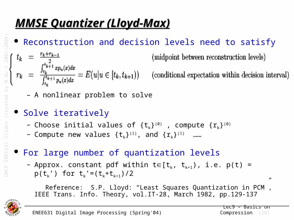
MMSE Quantizer (Lloyd-Max)MMSE Quantizer (Lloyd-Max)

Reconstruction and decision levels need to satisfy

– A nonlinear problem to solve

Solve iteratively– Choose initial values of {tk}(0) , compute {rk}(0) – Compute new values {tk}(1), and {rk}(1) ……

For large number of quantization levels– Approx. constant pdf within t[tk, tk+1), i.e. p(t) = p(tk’) for tk’=(tk+tk+1)/2

Reference: S.P. Lloyd: “Least Squares Quantization in PCM”, IEEE Trans. Info. Theory, vol.IT-28, March 1982, pp.129-137

UM

CP

EN

EE

63

1 S

lide

s (c

rea

ted

by

M.W

u ©

20

01

/20

04

)


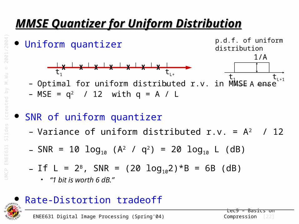
MMSE Quantizer for Uniform DistributionMMSE Quantizer for Uniform Distribution

Uniform quantizer

– Optimal for uniform distributed r.v. in MMSE sense– MSE = q2 / 12 with q = A / L

SNR of uniform quantizer

– Variance of uniform distributed r.v. = A2 / 12

– SNR = 10 log10 (A2 / q2) = 20 log10 L (dB)

– If L = 2B, SNR = (20 log102)*B = 6B (dB) “1 bit is worth 6 dB.”

Rate-Distortion tradeoff

t1 tL+1A

1/A

p.d.f. of uniformdistribution

t1 tL+1

UM

CP

EN

EE

63

1 S

lide

s (c

rea

ted

by

M.W

u ©

20

01

/20

04

)


Think More About Uniform QuantizerThink More About Uniform Quantizer

Uniformly quantizing [0, 255] to 16 levels

Compare relative changes

– x1 = 100 [96, 112) quantize to “104” ~ 4% change

– x2 = 12 [0, 16) quantize to “8” ~ 33% change

– Large relative changes could be easily noticeable by eyes!

UM

CP

EN

EE

63

1 S

lide

s (c

rea

ted

by

M.W

u ©

20

01

)


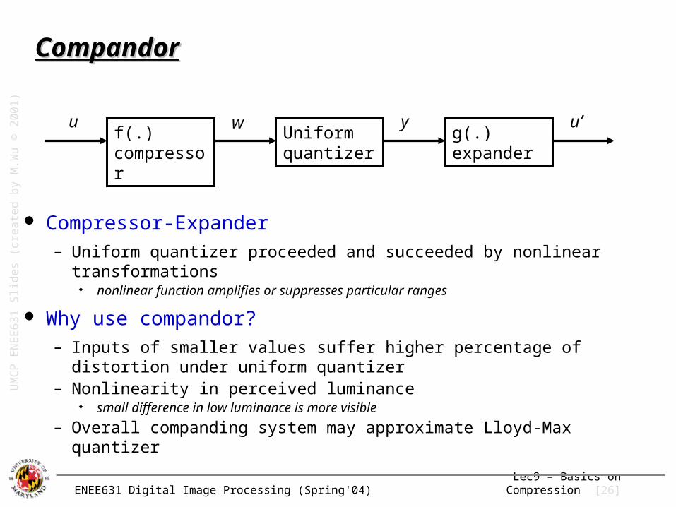
CompandorCompandor

Compressor-Expander– Uniform quantizer proceeded and succeeded by nonlinear transformations

nonlinear function amplifies or suppresses particular ranges

Why use compandor?– Inputs of smaller values suffer higher percentage of distortion under

uniform quantizer– Nonlinearity in perceived luminance

small difference in low luminance is more visible

– Overall companding system may approximate Lloyd-Max quantizer

f(.)compressor

g(.)expander

Uniform quantizer

u w y u’

UM

CP

EN

EE

63

1 S

lide

s (c

rea

ted

by

M.W

u ©

20

01

)


Quantization in Coding Correlated SequenceQuantization in Coding Correlated Sequence Consider: high correlation between successive samples

Predictive coding– Basic principle: Remove redundancy between successive pixels and only

encode residual between actual and predicted – Residue usually has much smaller dynamic range

Allow fewer quantization levels for the same MSE => get compression

– Compression efficiency depends on intersample redundancy

First try:

Any problem with this codec?

uQ (n)

Predictor+

eQ(n)

uP(n) = f[uQ(n-1)] DecodeDecode

rr

u(n)

Predictor

Quantizer_

e(n) eQ(n)

EncodeEncoderr

u’P(n) = f[u(n-1)]

UM

CP

EN

EE

40

8G

Slid

es

(cre

ate

d b

y M

.Wu

& R

.Liu

© 2

00

2)


Predictive Coding (cont’d)Predictive Coding (cont’d)

Problem with 1st try– Input to predictor are different at

encoder and decoder decoder doesn’t know u(n)!

– Mismatch error could propagate to future reconstructed samples

Solution: Differential PCM (DPCM)

– Use quantized sequence uQ(n) for prediction at both encoder and decoder

– Simple predictor f[ x ] = x– Prediction error e(n)– Quantized prediction error eQ(n)

– Distortion d(n) = e(n) – eQ(n)

uQ (n)

Predictor+

eQ(n)

uP(n)= f[uQ(n-1)]

DecodeDecoderr

EncodeEncoderr

u(n)

Predictor

Quantizer_

e(n) eQ(n)

+uP(n)=f[uQ(n-1)]

uQ(n)

UM

CP

EN

EE

40

8G

Slid

es

(cre

ate

d b

y M

.Wu

& R

.Liu

© 2

00

2)

Note: “Predictor” contains one-step buffer as input to the prediction


More on PredictorMore on Predictor

Causality required for coding purpose– Can’t use the samples that decoder hasn’t got as reference

Use last sample uq(n-1)– Equiv. to coding the difference

pth–order auto-regressive (AR) model – Use a linear predictor from past samples

– Determining the predictor coeff. (discuss more later)

)()()(1

neinuanup

ii

Line-by-line DPCM

– predict from the past samples in the same line

2-D DPCM

– predict from past samples in the same line and from previous lines

UM

CP

EN

EE

63

1 S

lide

s (c

rea

ted

by

M.W

u ©

20

01

)


Vector QuantizationVector Quantization

Encode a set of values together– Find the representative combinations– Encode the indices of combinations

Stages– Codebook design– Encoder– Decoder

Scalar vs. Vector quantization– VQ allows flexible partition of coding cells– VQ could naturally explore the correlation

between elements– SQ is simpler in implementation

From Bovik’s Handbook Sec.5.3

scalar quantization of 2 elements

vector quantization of 2 elements

UM

CP

EN

EE

63

1 S

lide

s (c

rea

ted

by

M.W

u ©

20

01

)


Outline of Core Parts in VQOutline of Core Parts in VQ

Design codebook– Optimization formulation is similar to MMSE scalar quantizer– Given a set of representative points

“Nearest neighbor” rule to determine partition boundaries

– Given a set of partition boundaries “Probability centroid” rule to determine representative

points that minimizes mean distortion in each cell

Search for codeword at encoder– Tedious exhaustive search– Design codebook with special structures to

speed up encoding E.g., tree-structured VQ

Reference: Wang’s book Section 8.6 A. Gersho and R. M. Gray, Vector Quantization and Signal Compression, Kluwer Publisher. R. M. Gray, ``Vector Quantization,'' IEEE ASSP Magazine, pp. 4--29, April 1984.

vector quantization of 2 elements

UM

CP

EN

EE

63

1 S

lide

s (c

rea

ted

by

M.W

u ©

20

01

/20

04

)


Summary: List of Compression ToolsSummary: List of Compression Tools

Lossless encoding tools– Entropy coding: Huffman, Lemple-Ziv, and others (Arithmetic coding)– Run-length coding

Lossy tools for reducing bit rate– Quantization: scalar quantizer vs. vector quantizer– Truncations: discard unimportant parts of data

Facilitating compression via Prediction– Convert the full signal to prediction residue with smaller dynamic range– Encode prediction parameters and residues with less bits

Facilitating compression via Transforms– Transform into a domain with improved energy compaction

UM

CP

EN

EE

63

1 S

lide

s (c

rea

ted

by

M.W

u ©

20

04

)

enee631 digital image processing (spring'04) basics on image compression spring ’04...

Documents

image compression spring

basics umcp enee631

enee631 spring04 section

enee631 s04

source compression

image restoration filtering

pcm coding

need compression