energy aware techniques for certain problems in wireless
TRANSCRIPT

Energy aware techniques for certain problems
in Wireless Sensor Networks
by
Kamrul Islam
A thesis submitted to the
School of Computing
in conformity with the requirements for
the degree of Doctor of Philisophy
Queen’s University
Kingston, Ontario, Canada
April 2010
Copyright c© Kamrul Islam, 2010
Abstract
Recent years have witnessed a tremendous amount of research in the field of wireless
sensor networks (WSNs) due to their numerous real-world applications in environ-
mental and habitat monitoring, fire detection, object tracking, traffic controlling,
industrial and machine-health control and monitoring, enemy-intrusion in military
battlefields, and so on. However, reducing energy consumption of individual sensors
in such networks and obtaining the expected standard of quality in the solutions
provided by them is a major challenge. In this thesis, we investigate several prob-
lems in WSNs, particularly in the areas of broadcasting, routing, target monitoring,
self-protecting networks, and topology control with an emphasis on minimizing and
balancing energy consumption among the sensors in such networks. Several inter-
esting theoretical results and bounds have been obtained for these problems which
are further corroborated by extensive simulations of most of the algorithms. These
empirical results lead us to believe that the algorithms may be applied in real-world
situations where we can achieve a guarantee in the quality of solutions with a certain
degree of balanced energy consumption among the sensors.
i

Acknowledgements
First of all, I thank Allah for his mercy and help without which this document would
not be possible. glorify the greatness and bounty of Allah who has bestowed on me
the strength and ability without which the document would not be possible.
I am grateful to my supervisors Prof. Selim G. Akl and Prof. Henk Meijer who
introduced me to the tremendously exciting field of research and guided me to the way
of innovation and novelty. Their invaluable ideas and profound research experience
kept me enthusiastic and optimistic all the way to the completion of this thesis. I
thank them for their many hours of patience for listening to my problems. Their
assistance, comments, constructive criticism and positive attitude helped me proceed
towards completing each step of the thesis.
I would like to acknowledge the support and facilities I received from the staff of
School of Computing and Queen’s University.
I am indebted to my father Late Md. Anowarul Islam for introducing me the
things I did not know and the utmost care I received from him. I pay my sincere
gratitude and profound love to my mother, Mst. Fazilatun Nessa, who put up with
hardships and kept patient to raise us (My brother, me and my sister).
Lastly, I thank my wife Mithila whose understanding, inspiration, and constant
support provided me with great optimism even in difficult situations while she took
ii

full care of our two beautiful sons Ayaan and Adib.
iii

Statement of Originality
I hereby certify that this PhD thesis is original and proper references are made wher-
ever I use ideas contributed by others.
iv

Table of Contents
Abstract i
Acknowledgements ii
Statement of Originality iv
Table of Contents v
List of Figures ix
Chapter 1:
Introduction . . . . . . . . . . . . . . . . . . . . . . . . . . 1
1.1 New Challenges . . . . . . . . . . . . . . . . . . . . . . . . . . . . . . 2
1.2 Problems and Energy Issues in Wireless Sensor Networks . . . . . . . 4
1.3 Outline of the Thesis . . . . . . . . . . . . . . . . . . . . . . . . . . . 12
Chapter 2:
Definitions and Model . . . . . . . . . . . . . . . . . . . . 14
Chapter 3:
Connected Dominating Sets . . . . . . . . . . . . . . . . . 21
3.1 Related Work . . . . . . . . . . . . . . . . . . . . . . . . . . . . . . . 22
v
3.2 Some Definitions . . . . . . . . . . . . . . . . . . . . . . . . . . . . . 24
3.3 A Distributed Algorithm for CDS . . . . . . . . . . . . . . . . . . . . 24
3.4 Algorithm and Analysis . . . . . . . . . . . . . . . . . . . . . . . . . 27
3.5 Conclusion . . . . . . . . . . . . . . . . . . . . . . . . . . . . . . . . . 38
Chapter 4:
Family of Connected Dominating Sets . . . . . . . . . . 39
4.1 A Motivating Example . . . . . . . . . . . . . . . . . . . . . . . . . . 40
4.2 Related Work . . . . . . . . . . . . . . . . . . . . . . . . . . . . . . . 43
4.3 Preliminaries and Problem Formulation . . . . . . . . . . . . . . . . . 44
4.4 A 3-local CDS Algorithm . . . . . . . . . . . . . . . . . . . . . . . . . 45
4.5 Theoretical Analysis . . . . . . . . . . . . . . . . . . . . . . . . . . . 49
4.6 Conclusion . . . . . . . . . . . . . . . . . . . . . . . . . . . . . . . . . 55
Chapter 5:
Domatic Partition . . . . . . . . . . . . . . . . . . . . . . 57
5.1 Introduction . . . . . . . . . . . . . . . . . . . . . . . . . . . . . . . . 58
5.2 Related Work . . . . . . . . . . . . . . . . . . . . . . . . . . . . . . . 61
5.3 Preliminaries and Definitions . . . . . . . . . . . . . . . . . . . . . . . 63
5.4 Algorithm for the Domatic Partition Problem . . . . . . . . . . . . . 64
5.5 Theoretical Analysis . . . . . . . . . . . . . . . . . . . . . . . . . . . 68
5.6 Simulations . . . . . . . . . . . . . . . . . . . . . . . . . . . . . . . . 71
5.7 Conclusion . . . . . . . . . . . . . . . . . . . . . . . . . . . . . . . . . 78
Chapter 6:
Target Monitoring . . . . . . . . . . . . . . . . . . . . . . 79
vi

6.1 Introduction . . . . . . . . . . . . . . . . . . . . . . . . . . . . . . . . 80
6.2 Related Work . . . . . . . . . . . . . . . . . . . . . . . . . . . . . . . 82
6.3 Preliminaries and Some Definitions . . . . . . . . . . . . . . . . . . . 84
6.4 The Algorithm . . . . . . . . . . . . . . . . . . . . . . . . . . . . . . 85
6.5 Theoretical Analysis . . . . . . . . . . . . . . . . . . . . . . . . . . . 88
6.6 Simulations . . . . . . . . . . . . . . . . . . . . . . . . . . . . . . . . 95
6.7 Conclusion . . . . . . . . . . . . . . . . . . . . . . . . . . . . . . . . . 98
Chapter 7:
Self Protection . . . . . . . . . . . . . . . . . . . . . . . . 99
7.1 Introduction . . . . . . . . . . . . . . . . . . . . . . . . . . . . . . . . 100
7.2 Related Work . . . . . . . . . . . . . . . . . . . . . . . . . . . . . . . 101
7.3 Minimum p-self-protection Subset Problem . . . . . . . . . . . . . . . 104
7.4 Theoretical Properties of Algorithm D . . . . . . . . . . . . . . . . . 109
7.5 Simulations . . . . . . . . . . . . . . . . . . . . . . . . . . . . . . . . 112
7.6 Conclusion . . . . . . . . . . . . . . . . . . . . . . . . . . . . . . . . . 115
Chapter 8:
Topology Control . . . . . . . . . . . . . . . . . . . . . . . 117
8.1 Introduction . . . . . . . . . . . . . . . . . . . . . . . . . . . . . . . . 118
8.2 Related work . . . . . . . . . . . . . . . . . . . . . . . . . . . . . . . 120
8.3 Preliminaries . . . . . . . . . . . . . . . . . . . . . . . . . . . . . . . 125
8.4 Local topology control algorithm (LTCA) . . . . . . . . . . . . . . . . 126
8.5 Analysis for random graphs . . . . . . . . . . . . . . . . . . . . . . . 132
8.6 Conclusion . . . . . . . . . . . . . . . . . . . . . . . . . . . . . . . . . 136
vii

Chapter 9:
Conclusion and Future Works . . . . . . . . . . . . . . . 138
Bibliography . . . . . . . . . . . . . . . . . . . . . . . . . . . . . . . . . 141
viii

List of Figures
1.1 A typical wireless sensor network. . . . . . . . . . . . . . . . . . . . . 3
3.1 Node 4 is black since CH(N [4]) = 1, 2, 3, 5 (shown in dashed line
segments) is not included in any of CH(N [1]), CH(N [2]), CH(N [3])
or CH(N [5]). The same applies to nodes 5 and 6. . . . . . . . . . . . 26
3.2 (a) After Phase I, B = 1, 2, 3, 4, 5, 6, 7, 8, 9, 10. (b) S consists of
nodes 4, 10. Additional node set is B ′ = 1, 6. (c) After Phase II
the solution is S∪C∪B′ = 1, 4, 5, 6, 10, where C = 5. The MCDS
consists of 1, 6. . . . . . . . . . . . . . . . . . . . . . . . . . . . . . 28
3.3 A Distributed algorithm for the CDS problem. . . . . . . . . . . . . . 29
3.4 Proof of Lemma 3.4.2. . . . . . . . . . . . . . . . . . . . . . . . . . . 32
4.1 Family of CDSs. . . . . . . . . . . . . . . . . . . . . . . . . . . . . . . 42
4.2 Phase I of the algorithm. . . . . . . . . . . . . . . . . . . . . . . . . . 46
4.3 Phase II of the algorithm. . . . . . . . . . . . . . . . . . . . . . . . . 48
4.4 Illustration of the algorithm to produce a family of CDSs. . . . . . . 49
ix

4.5 Illustration of Lemma 4.5.7. (a) An optimal algorithm chooses any
column of nodes as a CDS each time (shown in black), whereas our
algorithm (b) first chooses black nodes from each clique and then uses
at most two additional (shown in brown) nodes from each clique to
make them connectors between cliques. . . . . . . . . . . . . . . . . . 54
4.6 A counterexample showing that obtaining the maximum number of
disjoint CDSs does not always maximize α. . . . . . . . . . . . . . . . 56
5.1 (a) In this 3-connected graph (it is a general graph, not a UDG), we
have four disjoint dominating sets. Each dominating set is denoted by
the same digit. Hence the domatic partition of this graph is 4. (b) The
graph does not admit more than two disjoint dominating sets although
the minimum degree plus one is 3. . . . . . . . . . . . . . . . . . . . . 60
5.2 An algorithm for the domatic partition problem. . . . . . . . . . . . . 66
5.3 Disjoint dominating sets computation. D1, D2, and D3 are shown in
(a), (b), and (c) respectively. (d) D4 cannot be formed. Although the
algorithm tries to form D4, it abandons for not being successful. A
cross, ‘x’ means the formation of D4 is abandoned. . . . . . . . . . . 67
5.4 Showing the comparison between the average domatic partition (DP)
number returned by the algorithm and the average optimal DP number
(minimum degree of G plus 1) in different field sizes for each value of
n ∈ 100, 200, · · · , 1000. . . . . . . . . . . . . . . . . . . . . . . . . . 73
5.5 Showing the average minimum cardinality of dominating sets found by
our algorithm for different values of n. . . . . . . . . . . . . . . . . . 74
x

5.6 Showing the average maximum cardinality of dominating sets found
by our algorithm for different values of n. . . . . . . . . . . . . . . . . 75
5.7 A sample output with 200 nodes distributed on 400m x 400m square
field where both the optimal DP and the computed DP numbers are 6
(shown in 6 different colors). . . . . . . . . . . . . . . . . . . . . . . . 76
5.8 Showing standard deviations of DP numbers for different size of fields. 77
6.1 A sensor network in which three sensors can sense a target which falls
in their sensing range. . . . . . . . . . . . . . . . . . . . . . . . . . . 81
6.2 Nodes u1, u2, and u3 monitor target b and the monitoring sets are
Vi = ui, ∀i. . . . . . . . . . . . . . . . . . . . . . . . . . . . . . . . 88
6.3 For a target in the striped region (intersection of the five disks) we set
as active at most five nodes whereas only one node suffices. . . . . . . 89
6.4 A 2-local algorithm for the target monitoring problem. . . . . . . . . 90
6.5 If T (u) ∩ T (v) 6= φ then v ∈ N(u). . . . . . . . . . . . . . . . . . . . . 93
6.6 Average z values (optimal zopt values by solid lines and zalg by dashed
lines) for (a) 100 (b) 200 (c) 300 (d) and (e) 500 sensors. . . . . . . . 96
6.7 Showing standard deviations of zalg values for different number of tar-
gets and sensors. . . . . . . . . . . . . . . . . . . . . . . . . . . . . . 98
7.1 Minimum 1-self-protection and 2-self-protection subsets. . . . . . . . 104
7.2 Counterexample to the proof of Theorem 2 [77]. . . . . . . . . . . . . 106
7.3 Algorithm D for the p-protection subset. . . . . . . . . . . . . . . . . 109
7.4 Showing average sizes of p-protection subsets for different values of
n ∈ 100, 200, · · · , 500 and p ∈ 1, 2, 3. . . . . . . . . . . . . . . . . 114
xi

7.5 Showing average approximation ratios for p-protection subsets for dif-
ferent values of n. . . . . . . . . . . . . . . . . . . . . . . . . . . . . . 115
7.6 Showing standard deviations of the sizes of p-protection subsets for
different values of n. . . . . . . . . . . . . . . . . . . . . . . . . . . . 116
8.1 The XTC algorithm produces a disconnected graph (b) with a small
error in the estimated distances between nodes in the graph shown in
(a). (c) If a incorrectly estimates c’s actual position then the GG can
have new edge ac′. . . . . . . . . . . . . . . . . . . . . . . . . . . . . 125
8.2 The LTCA algorithm. . . . . . . . . . . . . . . . . . . . . . . . . . . 127
8.3 Proving that the subgraph obtained by LTCA is connected. . . . . . . 128
8.4 Situations like the ones shown in (b) and (c) are indistinguishable
from each other and hence intersections cannot be removed with only
connectivity information: labels indicate the corresponding ids of the
nodes. As illustrated in (a) (right), we can obtain a planar subgraph
from a clique (left), assuming u has the lowest id in the clique. . . . . 131
8.5 The UDG (left), the Gabriel graph (center) and GTC of 600 nodes
placed randomly and uniformly are shown, where the minimum dis-
tance between any two nodes is at least 0.4 unit. . . . . . . . . . . . . 133
xii

8.6 Spanner ratios of the GG and GTC w.r.t the Euclidean metric (left).
The solid (resp. the dashed) line represents the spanner ratio of GG
(resp. GTC). Mean values are plotted in black and max values in gray.
Spanner ratios of the GG and GTC w.r.t the energy metric is shown
(right). The solid (resp. the dashed) line represents the energy-spanner
ratio of the GG (resp. GTC). Mean values are plotted in black and
max values in gray. Since the GG contains an energy-minimal path
between any pair of nodes its energy-spanner ratio is one (solid line).
So its max and mean values coincide. . . . . . . . . . . . . . . . . . . 135
8.7 Average degree of the GG and GTC in random graphs of different sizes.
The dashed and the solid lines denote the sparseness of the GG and
GTC respectively. As can be seen from the figure, the average degree
of GTC is always smaller than that of the GG in all the instances of
different sizes of graphs. . . . . . . . . . . . . . . . . . . . . . . . . . 136
8.8 Showing standard deviations of spanner ratios of the algorithm for the
Euclidean and energy metrics. . . . . . . . . . . . . . . . . . . . . . . 137
xiii

List of Notations
V a set of n nodes representing n points (sensors) in general
position in the plane
E a set of edges representing links among the sensors
vivj an edge connecting nodes vi and vj
WSN Wireless Sensor Network
UDG Unit Disk Graph
G G is a UDG with node set V and edge set E
GG Gabriel Graph
RNG Relative Neighborhood Graph
MIS Maximal Indpendent Set
CDS Connected Dominating Set
MCDS Minimum Connected Dominating Set
MST Minimum Spanning Tree
DP Domatic Partition
CH Cluster Head
CH(X) Convex hull of the set of X points in the plane
Nk(u) u′s k-hop neighbor set excluding u
Nk[u] u′s k-hop neighbor set including u
Di Dominating Set at iteration i

Chapter 1
Introduction
Wireless sensor networks (WSNs) offer a wealth of capabilities in interacting with the
physical world by collecting, transmitting, and processing data from the environment
and responding accordingly. Typical applications of WSNs include environmental
monitoring (such as fires, floods, earthquakes, etc.), infrastructure protection, in-
telligent homes, military battlefield surveillance, rescue operations, observation of
chemical and biological processes, and so on.
A WSN consists of a number of small battery-powered sensors, each equipped with
limited on-board processing, bandwidth, sensing, transmission and receiving devices.
Through the transmitting device, a sensor can transmit a signal (typically radio
signals) to a finite distance (known as the transmission radius) and all sensors within
this distance can receive the signal by their receiving antennae. Since a radio signal
is omnidirectional, one can assume the transmission area of a signal is a circular disk
centered at the sensor originating the signal, whose radius is equal to the transmission
radius.
As there is no physical connection between any two sensors in a WSN, a virtual
1

CHAPTER 1. INTRODUCTION 2
link between them is established if they are located within each other’s disk, i.e.,
they are capable of sending and receiving their signals directly. Furthermore, with
its sensing device, a sensor can sense certain environmental phenomena such as tem-
perature, light, pressure, humidity, and the presence of some physical objects (e.g.,
animals or vehicles and so on) within a certain range known as the sensing radius.
Typically, a sensors’s sensing radius is equal to its transmission radius. Thus, after
the deployment of sensors, an adhoc (infrasturcture-less) WSN is formed which then
begins to operate independently without any external control. However, the underly-
ing physical topology of such networks is dependent on the distribution of the sensors
and their transmission radii.
In general, a WSN is used to allow a collection of unattended sensors deployed at
arbitrary locations to form a virtual network and provide cooperatively and collec-
tively sensed data about some events of interest to the base station (also called the
sink). The sink eventually processes the gathered data transmitted by the network to
obtain an overall picture of the environment and takes decisions accordingly. Figure
1.1 shows a typical WSN.
1.1 New Challenges
Because of their flexibility, efficacy, low-cost, and ease of deployment, WSNs are
gaining attention and expanding their domain of applications. Unlike traditional and
electrically-powered wired computer networks, a WSN comes with a unique set of
resource constraints such as finite on-board battery power, limited processing ability,
and constrained communication bandwidth. Moreover, a typical WSN is expected
to work without human intervention for a long time period. These features present

CHAPTER 1. INTRODUCTION 3
transmissionradius
sensor
base station (sink)
Figure 1.1: A typical wireless sensor network.
unique challenges to come up with new paradigms that can harness the benefits of
numerous applications of WSNs.
As sensors are battery-powered, consideration of energy efficiency is of paramount
importance in WSNs. Due to the energy constraints of sensors, communication pro-
tocols and hardware architectures for WSNs necessitate an energy-aware design to
ensure the longevity of the network. Algorithms are expected to address the power
constraint of WSNs without compromising the standard of the solution provided by
them.
As each transmission of data over a link in WSNs consumes a certain amount
of energy (energy consumption is directly proportional to at least the square of the
Euclidean distance of the link), special care must be taken so that protocols minimize
the amount of communication. Local collaboration among sensors, redundant data
suppression, data compression, and avoidance of direct transmission to long-distant
sensors are some of the important factors that influence algorithm designers to devise

CHAPTER 1. INTRODUCTION 4
novel distributed, scalable and energy-efficient solutions for WSNs. Moreover, the
dynamic nature of WSNs, e.g., sensor and link failures (due to physical damage
or power failure of sensors) requires algorithms to be robust and resilient in such
situations.
1.2 Problems and Energy Issues in Wireless Sen-
sor Networks
As mentioned before, reducing energy consumption on individual sensors (or just
nodes, henceforth we use sensors and nodes interchangeably) in the network and ob-
taining the expected standard of quality in the solutions provided by such networks is
a major challenge. In this thesis, we address a number of problems arising from var-
ious applications of WSNs with a view to finding efficient polynomial-time solutions
while emphasizing the energy minimization issue of such networks. The problems
considered fall in the broad categories of broadcasting, clustering, monitoring, and
topology control of WSNs.
We mainly focus on devising distributed (and local) algorithms for these problems,
where individual nodes execute algorithms on their own to compute solutions to a
problem of a global nature. A distributed algorithm is one where nodes individually
execute the same algorithm and make decisions accordingly without knowing the
global topology of the network. However, in some distributed algorithms, it is allowed
that nodes may know a little global information (e.g., the number of sensors in the
network and/or the maximum degree of the underlying graph). A more strict version
of the distributed algorithm is known as the local algorithm. Informally, in a local

CHAPTER 1. INTRODUCTION 5
algorithm, a node is allowed to communicate only with its neighbors, which are at
most a constant hop away from it, to make decisions during the execution of the
algorithm (more about local algorithms is described later in this chapter).
Unlike centralized systems, the distributed and local approaches relieve sensors
from sending their information (e.g., ids, geographic positions, neighborhood infor-
mation, covered areas, and so on) to a central base station which runs the algorithm
and returns the results to the sensors. Sending information to a base station is energy-
consuming and generally not scalable. However, we consider the following problems
in the thesis:
1.2.1 Broadcasting Issues
Broadcasting is an operation by which a message, generated by a node in the network,
is forwarded to all other nodes in the network. Following a simple flooding approach
to do this is inefficient. This is because a lot of unnecessary message transmissions
(or just transmissions) are generated and relayed in the network, which in turn,
causes nodes to dissipate their valuable energy quickly. Thus we need to devise
energy-efficient algorithms that can avoid or at least reduce the amount of redundant
transmissions.
Virtual backbone
Establishing a virtual backbone in WSNs, which can be seen as an analogue of the
fixed communication infrastructure in wired networks, helps reduce the number of
retransmissions of the energy-constrained sensors. In a virtual backbone, only a
“small” number of nodes in the network are engaged in transmissions. Basically, a

CHAPTER 1. INTRODUCTION 6
virtual backbone consists of a subset of nodes in the network which are responsible for
relaying messages throughout the network. The connected dominating set (CDS) is
one of the earliest and most popular structures proposed as a candidate for a virtual
backbone in wireless networks [18]. Since the work of Das et. al. [18], an extensive
research effort has been put into finding small-sized CDSs in WSNs. The smaller
the size of a CDS, the fewer the number of transmissions in the network. Chapter
3 studies the problem of computing CDSs in a distributed way and discusses other
relevant issues.
Family of Connected Dominating Sets
We make an important observation regarding finding small-sized or even optimal
CDSs in WSNs. Although the general focus of research for broadcasting algorithms
is to obtain small cardinality CDSs, generating a single CDS (even if it is optimal)
and using it all the time causes the nodes in the CDS to run out their energy faster
than other nodes (which are not in the CDS). This is because the nodes in the CDS
are responsible for forwarding messsages in the network on behalf of other nodes,
whenever any node in the network has some messages to broadcast. Considering
this important aspect, we study the problem of computing a family of CDSs in a
distributed manner such that only one CDS is active for a certain period of time and
other nodes can be put in the energy-efficient sleep mode.
Thus, using the CDSs iteratively, we can expect to substantially reduce the energy
consumption of the individual nodes by repeatedly switching them back and forth
from the active to the sleep mode and make the lifetime of the network longer. By
the lifetime of a WSN, we mean the elapsed time between the deployment of the

CHAPTER 1. INTRODUCTION 7
sensors and the time when the first sensor runs out of energy. Keeping this in mind,
we aim at studying the problem of locally generating a family of non-trivial CDSs in
WSNs with the goal to minimize the number of participations of individual nodes in
these sets. Chapter 4 deals with this problem and investigates special cases where
the algorithm achieves ‘good’ results.
1.2.2 Clustering
Clustering is a heavily studied topic [26, 21, 22, 27, 53, 4, 74] in the WSNs community,
where the goal is to divide the whole network in a number of clusters (not necessarily
disjoint) and select a node as a cluster head (CH) from each of the clusters. Each
such CH is supposed to be active and do all the coordination works, e.g., sensing,
data gathering, and transmitting data on behalf of the cluster to the base station,
while the remaining nodes in the cluster can go into the sleep mode. One of the basic
problems in clustering is to minimize the number of CHs under the condition that for
any node in the network either it is a CH or directly connected to at least one CH.
This would leave most of sensors in the energy-efficient sleep mode. This problem is
also known as the minimum dominating set problem.
However, as the set of CHs (even the minimum set of CHs) is busy all the time
for sensing, processsing, and transmitting data, they quickly run out of energy, while
other nodes (which are not CHs) are left with considerable amount of energy. This
causes a significant imbalance in the energy reserve in the nodes and reduces the
network lifetime. One possible way to overcome this situation is to find a family of
disjoint sets of CHs and make them active iteratively such that energy consumption
is balanced among the nodes in the network.

CHAPTER 1. INTRODUCTION 8
Disjoint Dominating Sets
In the context of WSNs (considering the above circumstance), we address the follow-
ing problem: “Given a WSN, find the maximum number of disjoint dominating sets”.
A dominating set of a graph is a subset of nodes such any node in the graph either
is in the subset or a neighbor of some node in the subset. Finding the maximum
number of disjoint dominating sets in a graph is also known as the Domatic Partition
problem. Although the domatic partition problem is NP-hard in general graphs, it
is unknown whether the same is true for unit disk graphs. Chapter 5 discusses the
problem of finding the maximum number of disjoint dominating sets in WSNs (a
WSN is modeled as a unit disk graph) and presents a centralized algorithm to solve
the problem.
1.2.3 Target Monitoring
Monitoring (also called coverage) is one of the important and extensively studied
topics in sensor networks [8, 10, 11, 47, 31, 71, 78]. In general, the main goal of
research in this line is to devise scheduling algorithms such that individual sensors in
the network are assigned time-slots which indicate to them during which time-slots
they will be active and during which time-slots they will sleep. Given a WSN which
monitors certain targets, it is sometimes possible to find only a subset of the sensors
and engage them to do the same monitoring activity. Thus, instead of making all
nodes active for this purpose (which is obviously redundant), we can choose possibly
a small subset which can guarantee the same monitoring. This observation leads
researchers to devise efficient algorithms such that at any time only a small number
of nodes are made active to monitor all the targets in question.

CHAPTER 1. INTRODUCTION 9
Chapter 6 investigates the following target monitoring problem. Given a set of
stationary targets T and a set V of sensors, the problem asks for generating a family
of subsets of sensors called the monitoring sets, such that each monitoring set mon-
itors all targets. The monitoring sets are iteratively made active in order to provide
continuous monitoring to the targets. The objective of this problem is to maximize
the number of monitoring sets and minimize the maximum number of participations
of a sensor in these monitoring sets. This chapter provides a local technique to solve
the problem approximately, discusses theoretical results, and compares experimental
results with the theoretical bounds.
1.2.4 Self Protecting WSNs
We study an interesting problem which deals with providing sensors with a level of
protection by other sensors. Since sensors provide monitoring to targets, it is often
necessary to give them a level of protection (by other sensors) such that sensors can
take certain actions when attacks are targeted on them. One natural idea is to monitor
sensors by their neighbors such that the neighbors can inform the base station when
other sensors are in danger (or not working due to malfunction). We elaborate on
this in the following.
Sometimes it may be required to know whether every sensor in the network is in
good health to render its tasks. Since a bad sensor, i.e., a malfunctioning or dying
out sensor cannot inform the base station of its condition, the targets monitored by
the bad sensor become unprotected and the system has no way to know about this
vulnerability. In that case, we need to find a subset of sensors whose function is
to monitor other sensors, such that when any sensor (including themselves) fails or
CHAPTER 1. INTRODUCTION 10
cannot function properly these sensors will notify the base station of the situation.
The base station then takes appropriate actions, such as, deploying additional nodes
in replacement of the non-functioning ones to provide continuous protection to the
targets.
Keeping this in mind, the p-self-protection subset problem has been formally in-
troduced in [79]. The p-self-protection subset problem is defined to be a subset of
nodes such that for any node in the network there are at least p nodes from the subset
that monitor it. Chapter 7 studies the problem of p-self-protection (p ≥ 1). That
chapter begins by giving a counterexample to the algorithm [77], and then provides a
fast and distributed algorithm to approximately solve the p-self-protection problem.
1.2.5 Topology Control Problems
Topology control is one of the pivotal problems which has received a lot of attention
due to its numerous applications in WSNs such as coverage, connectivity, and routing
[44, 45, 48, 75, 84, 50, 49, 63, 65, 64, 80, 81, 19, 32, 6]. The main idea is to obtain a
subgraph from the underlying network by removing some (possibly redundant) links
in order to enhance the overall performance of the network in some ways.
Topology control algorithms, in general, deal with finding a suitable structure
(subgraph) of the given graph. This resulting subgraph is expected to have cer-
tain features (e.g., connectedness, planarity, sparseness, bounded-degree, and spanner
property, etc.) which mainly facilitate routing and other decisions in the network.
Finding a topology with the above features has certain advantages. First, a num-
ber of routing algorithms including the well-known GPSR routing algorithm [12] can
only be applied if and only if the network topology is planar. Second, by eliminating a

CHAPTER 1. INTRODUCTION 11
number of links, we can substantially reduce the burden of the nodes by letting them
keep only a subset (possibly small) of their neighbors. The smaller the neighborhood,
the faster the information processing of a node. Having a few neighbors also causes
a small number of transmissions and helps prolong the lifetime of the network by
limiting the number of retransmissions. Topology algorithms tend to remove longer
links in the network and keep smaller ones since long links consume more power than
shorter links for transmission (recall that the power spent on a link for a transmission
is directly proportional to at least the square of the length of that link). This saves
energy in the long run for routing and thus helps extend the network’s lifetime.
Chapter 8 investigates the topology control problem. It begins by showing cases
where a slight error in the exact geographic position, and/or the distances between
neighboring sensors, can make algorithms yield unwanted results (e.g, a disconnected
subgraph). A robust and resilient local algorithm with realistic assumptions is pre-
sented in the chapter, which is supposed to provide an ‘acceptable’ performance in
average cases. This chapter provides theoretical and experimental results.
1.2.6 Contribution of the Thesis
As centralized algorithms may not be suitable in large WSNs due to scalability and
energy issues, our aim in this thesis is to design energy-efficient distributed and local
algorithms to address the aforementioned problems. We devise distributed (or local)
solutions which are fast, scalable, and can be easily implemented in WSNs for the
problems except for the domatic partition problem, where we provide a centralized
algorithm.

CHAPTER 1. INTRODUCTION 12
Thus the contributions of the thesis are:
1. Designing and analyzing a fast, distributed and constant-approximation algo-
rithm for the connected dominating set problem.
2. Solving the energy consumption issue of the sensors in a balanced way by
generating a set of connected dominating sets in a distributed fashion.
3. Developing a technique (centralized) for the problem of approximately finding
the maximum number of dominating sets in unit disk graphs.
4. Presenting a local solution to the target monitoring problem.
5. Providing a distributed constant-approximation algorithm for the self-protection
problem.
6. Introducing a fast, easily implementable local algorithm for the topology control
problem in WSNs.
1.3 Outline of the Thesis
The rest of the thesis is organized as follows. In Chapter 2 we provide definitions
and assumptions that are used throughout the thesis. Chapter 3 discusses the CDS
problem and presents an algorithm to solve it. As a continuation of this problem,
Chapter 4 begins with an example that sheds light on the issue of having multiple
CDSs instead of just a single CDS and shows a way of generating a family of dif-
ferent CDSs. It also explores some interesting relationships between vertex-cuts and
the number of CDSs of a graph. The clustering problem, specifically the domatic
partition problem is studied in Chapter 5 and a centralized method is presented to
solve the problem. In Chapter 6, we define the target monitoring problem and give

CHAPTER 1. INTRODUCTION 13
a local algorithm towards solving it. The self-protection in WSNs is described and a
distributed technique to handle the problem is provided in Chapter 7. Chapter 8 is
devoted to discussing the topology control problem which begins by showing a coun-
terexample to some previous work and presents a fast local algorithm for it. Finally,
Chapter 9 provides a summary of the results and concludes with a number of open
problems.
In this thesis, I do not include a separate “Previous Work” chapter since each
chapter will include a section concerning previous work on the problem addressed in
that chapter.

Chapter 2
Definitions and Model
In this chapter, we define some terms which will be used thoroughout the thesis.
However, there are certain terms and notations which are defined in the corresponding
chapters according to their relevance.
2.0.1 Graph Terminology and other
We begin with some terminology regarding graphs. Assume a set of sensors are
deployed randomly and uniformly in the plane. We model the wireless network formed
by the sensors as a geometric undirected graph G = (V, E), where V = v1, v2, · · · , vn
denotes the set nodes (sensors) and there is a link between two nodes vi and vj,
vivj ∈ E, if the Euclidean distance between them is at most 1. In other words, G
is known as a unit disk graph (UDG). Unless otherwise mentioned, henceforth we
assume G is a UDG and connected and the number of nodes in G is denoted by
n = |V |.
The hop-distance between two nodes vi and vj in G is the minimum number of
14
CHAPTER 2. DEFINITIONS AND MODEL 15
edges between them and denoted by d(vi, vj). Also d(vi, vj) refers to the length of the
shortest path between vi and vj. The diameter Diam(G) is defined as the maximal
hop-distance between any two nodes in G, i.e., Diam(G)=maxu,v∈V d(u, v). If it is
clear from the context then we use distance instead of hop-distance.
The neighborhood of a node u ∈ V , denoted by N(u), is the set of nodes that are
u′s direct neighbors (not including u) in G. We use N [u] to include u in the neighbor
set. Formally, the neighborhoods of u are defined as
N(u) = v|uv ∈ E
N [u] = N(u) ∪ u.
In the distributed setting, we extend the definition of neighborhood in some depth.
For some constant integer k ≥ 1, the k-neighborhood Nk(u) of a node u is defined as
the set of all nodes which are at most k-hops away from u. That is,
Nk(u) = v|d(u, v) ≤ k.
Similarly Nk[u] is defined. For simplicity, we use N(u) = N1(u). The degree deg(u)
of node u is the number of direct neighbors it has, i.e., deg(u) = |N(u)|. The maximal
and minimal degrees in G are defined as ∆ =maxu∈V deg(u) and δ =minu∈V deg(u),
respectively. Each node u has a unique integer id, id(u) of size O(log n).
We call two nodes u, v ∈ V independent if uv /∈ E. A subset I ⊆ V is called an
independent set if all pairs of nodes in I are independent. Set I is called a maximal
independent set (MIS) if no independent set T ⊃ I exists. A subset D ⊆ V is a

CHAPTER 2. DEFINITIONS AND MODEL 16
dominating set if each node u ∈ V is in D or adjacent to some node v ∈ D. If D
induces a connected subgraph, then D is called a connected dominating set (CDS).
A CDS with minimum cardinality is called a minimum connected dominating set
(MCDS).
In this thesis, we study some combinatorial optimization problems for which we
provide distributed algorithms. Since most combinatorial optimization problems are
NP-hard, polynomial-time algorithms designed to solve them provide only approxi-
mate solutions. The quality of an approximate solution can be measured by comparing
it with the optimal solution. Consider a minimization problem. Let ALGI denote the
value of the solution generated by algorithm A for all inputs I. If OPTI is the value
of the optimal solution for I, then the approximation factor (or ratio) α of algorithm
A is given by,
α = maxI
ALGI
OPTI
for all possible input I. For a maximization problem, the approximation ratio is
similarly defined as α=maxIOPTI
ALGI.
Finally, we use the notation log∗ n, which is the number of times the logarithm
function must be iteratively applied before the result is less than or equal to 1.
2.0.2 Computational Model
Most distributed systems consist of a set of nodes which are interconnected in some
way that permits them to cooperatively exchange information among nodes in order
to solve certain problems. Note that distributed systems are the opposite of the
centralized system where a single entity, knowing the whole topology of the system,

CHAPTER 2. DEFINITIONS AND MODEL 17
is responsible for solving the problem. However, in a distributed system each of the
nodes has a certain degree of autonomy allowing them to execute their own protocol,
share the results with neighbors to produce solutions for some applications. There
are two basic models that form the basis of most distributed systems, namely the
message passing and the shared memory models [61]. In the shared memory system,
nodes do not communicate with each other directly. Instead, the model assumes the
existence of a common memory storing variables that are shared (read and write) by
all nodes in the system. In contrast, the message passing model treats communications
explicitly. Whenever a node wants to speak with another, it must send a message to
its neighbors which may relay the message to their neighbors and so on to eventually
reach the intended receiver. The information is sent and received using the underlying
communication media (wired or wireless).
In the thesis, we follow the message passing model. We assume communication
to be synchronous for all the distributed and local algorithms. In synchronous sys-
tems, time is divided into rounds and in each round every node can do the following
three things: it can send a unique message to each of its neighbors, receive messages
from its neighbors, and perform some local computation based on the information
received in previous rounds. Local computation is assumed to take negligible time as
compared to the message transmission time, so in synchronous systems, local com-
putation time is reasonably small [61]. Thus the time complexity of a synchronous
distributed algorithm is defined as the number of rounds until all nodes terminate.
In general, all proposed algorithms in synchronous systems neglect local computation
time (assuming this model allows nodes to compute a ‘computable’ function) and de-
rive a time complexity bound by the number of communication rounds it takes in the

CHAPTER 2. DEFINITIONS AND MODEL 18
worst-case execution. Similarly the message complexity of a synchronous distributed
algorithm is defined as the total number of messages generated by the algorithm in
the worst-case scenario.
The size of a message (that is, the number of bits contained in each of them) in
distributed synchronous systems plays an important role in message passing models.
The question of message sizes gives rise to two fundamental limitations in message
passing networks, namely, LOCAL and CONGEST [54, 59, 61] which differ in the
way of how much information (bits) should be included in a single message. We
elaborate on them in the following.
2.0.3 Local Algorithms
The LOCAL model, also known as Linial’s free model [54], places no restriction on
the size of a single message, that is, a node can send an arbitrarily large message to
its neighbors in any communication round. This model also assumes that communi-
cation is synchronous and that all the nodes wake up simultaneously and start the
execution of the protocol at the same round. Since the message size is unlimited,
congestion or bottlenecks have no influence on an algorithm’s time or message com-
plexity. However, one powerful aspect of the LOCAL model is that a node in some
distributed algorithm is able to know its k-neighborhood exactly in k communication
rounds. Since the message size is unbounded, a node can have all information (e.g.,
ids and interconnections) of all nodes which are at most k-hops away in k rounds.
Collecting the complete k-hop neighborhood is possible when each node sends its
complete information (in its arbitrary long single message) to all neighbors at every
round. This model gives rise to the definition of local algorithms. A distributed

CHAPTER 2. DEFINITIONS AND MODEL 19
algorithm is called a k − local algorithm if
1. each node collects its k-neighborhood information (ids, and neighborhood in-
formation) in k communication rounds and
2. it produces the output by performing only local computation with the infor-
mation collected (no communication required). (Recall that local computation time
is negligible) [57].
In the LOCAL model, every computable problem can be solved in Diam(G)
time since this is the time required for any node to learn the entire topology of the
underlying graph.
On the other hand, the goal of the CONGEST model is to limit the message
size and consider the aspects of congestion and volume of communications. Since the
LOCAL model abstracts away some difficulties and challenging issues arising in the
networks by making the message size long, the CONGEST model tries to capture
the issues of congestion and bottlenecks by limiting the message size to O(log n) bits.
That is, every node u ∈ V can send a message of size O(log n) bits to each of its
neighbors v ∈ N(u) at every round. Because of this restriction, each node is now
able to send at most a constant number of node identifiers in each message to its
neighbors. Given this limited message size, many problems on the complete network
graph (e.g., the Minimum Spanning Tree) which can be solved optimally relatively
easily in the LOCAL model becomes non-trivial in this model [57].
In the thesis, we will consider the LOCAL model (synchronous model with un-
bounded messages and local computations). As described before, in the LOCAL

CHAPTER 2. DEFINITIONS AND MODEL 20
model, at each round a node can send a unique message to each of its neighbors.
However, in the context of WSNs, when a node sends a message, it is broadcast to
all its immediate neighbors. That is, in WSNs, instead of sending a separate message
to each of its neighbors, a node sends a single message to all its neighbors. Thus
our model (we name it, LOCALS) does not deviate from the LOCAL model and the
computational powers of LOCAL and LOCALS are the same.

Chapter 3
Connected Dominating Sets
Connected dominating sets (CDSs) [13, 28, 16, 15, 56, 5, 68, 82, 70, 47, 83, 37] are
probably the most common way of constructing virtual backbones for broadcasting
operation in WSNs. This is because such backbones are guaranteed to reduce unnec-
essary message transmissions or flooding in the network. In this chapter we propose a
simple distributed algorithm to construct a small -sized CDS. Considering the nodes
deployed in the plane, our main idea is based on the computation of convex hulls of
nodes (nodes are considered points in the plane) in a distributed manner and a simple
coloring scheme, which produces a CDS in UDGs whose size is at most 50.54∗|MCDS|,
where |MCDS| is the size of a minimum CDS. To the best of our knowledge, this is a
significant improvement over the best published results in reducing the approximation
factor [13]. We also analyze geometric grids and trees to compute the exact approxi-
mation ratios for the problem and show that the algorithm produces an MCDS if the
graph is a tree and in the case of grids the approximation factor is 2.
The rest of the chapter is organized as follows. Section 3.1 presents related work.
In Section 3.2 we provide definitions and assumptions that are used throughout the
21
CHAPTER 3. CONNECTED DOMINATING SETS 22
chapter. The main idea of the distributed algorithm is described in Section 3.3. We
analyze the algorithm and give some theoretical results including time and message
complexities of the algorithm in Section 3.4. We conclude in Section 3.5.
3.1 Related Work
Guha and Khuller [28] studied the MCDS problem and showed that this problem is
NP-hard in arbitrary undirected graphs. They present a centralized approximation
algorithm which guarantees a O(log n) approximation factor, where n is the number
of nodes in the graph. Later it was shown in [16] that computing an MCDS is
NP-hard even for UDGs. The first centralized method towards solving this problem
achieves a 10-approximation factor and was given by Marathe [56]. Cheng et. al [15]
presented a polynomial-time approximation scheme that guarantees an approximation
factor of (1 + 1/s) with running time of nO((s log s)2), s > 0. However, in reality,
centralized algorithms may not be preferred for large networks because of their power
consumption. Therefore, distributed algorithms are sought to find an approximate
MCDS in such networks. Several distributed approximation algorithms exist in the
literature, some of the earlier attempts include the works of Stojmenovic and Xiang-Li
[70, 47, 83] which distributedly construct a CDS of size n/2 times that of an MCDS.
Alzoubi et al. [2] proposed the first distributed algorithm guaranteeing a constant
approximation factor for the CDS based on MIS in UDGs. The main features of their
distributed algorithm include an approximation factor of 8, O(n) time complexity,
and O(n log n) message complexity. One of the important results established in that
paper, is an Ω(n log n) a lower bound on the message complexity of any distributed
algorithm for nontrivial CDSs.
CHAPTER 3. CONNECTED DOMINATING SETS 23
However, the algorithm in [2] suffers from the construction of a spanning tree in
wireless networks, which is expensive since the time complexity is Diam(G) in which
case a node “needs to” know the whole topology of the network. Building a spanning
tree and maintaining a CDS in large and volatile WSNs with common node and link
failures incur a significant number of retransmissions and communication overhead.
Later, Alzoubi et al. came up with a constant factor distributed algorithm [1] that
does not rely on the construction of spanning trees. However, the algorithm produces
a CDS with size at most 192∗|MCDS|+48. Lately, Funke et al. [23] gave a distributed
algorithm which provides an approximation factor of 6.91 and outperforms all other
approximation factors of previous distributed algorithms. Although the factor is
small, the time complexity of their algorithm is still Diam(G), which is O(n) in the
worst-case.
In an attempt to obtain a small constant factor, a distributed algorithm is pro-
posed in [51] which produces a CDS with size at most 172 ∗ |MCDS| + 33 in UDGs.
Subsequently, the next level of reduction in the constant factor was achieved by the
distributed algorithm in [14], where the factor is 147 (specifically, 147∗ |MCDS|+43).
Recently D. Chen et al. managed to achieve even a smaller constant factor by a sim-
ple distributed algorithm. The cardinality of the CDS produced by their algorithm
is at most 76 ∗ |MCDS|+ 19. Here, we present a technique that reduces this constant
factor to 50.54 that is, it produces a CDS with size at most 50.54 ∗ |MCDS|. We ana-
lyze special classes of graphs, for example, trees and grids, where the approximation
ratios obtained by our algorithm are 1 (optimal) and 2, respectively.

CHAPTER 3. CONNECTED DOMINATING SETS 24
3.2 Some Definitions
Recall that nodes are deployed in the plane and the network is modeled by an undi-
rected graph G = (V, E), where a link uv ∈ E between two nodes u, v ∈ V exists if
they are within their transmission range, which is normalized to 1. We use a com-
putational geometry idea called the convex hull in our algorithm. The convex hull of
a set of points in the plane is defined as the smallest convex polygon that includes
all the points in the set such that each point is either a corner of the convex hull or
lies inside it. The convex hull of N(u) is denoted by CH(N(u)). We say CH(P ) of
some point set P ⊆ V is completely included (or just included) in CH(Q) of point
set Q ⊆ V if CH(P ) ⊆ CH(Q).
3.3 A Distributed Algorithm for CDS
In this section we present a simple algorithm for computing a CDS in G based on
the computation of convex-hulls of the 1-hop neighborhood of individual nodes and a
coloring scheme of the nodes of G. There are three colors, namely ‘black’, ‘grey’ and
‘white’. Initially all nodes are white.
Here we outline the algorithm (call our algorithm A):
The algorithm consists of two phases (Phase I and Phase II). In Phase I, we distribut-
edly form a primary CDS denoted by B, which is pruned in the next phase (II) to
generate the final CDS denoted by CDS∗ (CDS∗ is the solution we are looking for).
After the execution of Phase I, all nodes change their respective colors and become
either black (if the node belongs to B) or grey (otherwise).
In Phase II, first we prune the set B of black nodes. In order to do so, we apply a

CHAPTER 3. CONNECTED DOMINATING SETS 25
distributed MIS algorithm in B. Let the set of MIS nodes returned by the algorithm
be S ⊆ B. Although an MIS is a dominating set in a graph, the subset S is not a
dominating set in G since S is obtained from the nodes in B (not from the nodes V ).
Then we form a dominating set in G consisting of nodes in S and a set B ′ of additional
nodes (B′ ⊆ (V \ S)). Thereafter, a set C of connectors is selected from V \ S to
connect the nodes in S such that S ∪ B ′ ∪ C forms the desired CDS∗. Following is a
detailed description of the two phases of algorithm A:
Phase I (Coloring nodes):
Initially all nodes are white. Each node u locally computes the convex hull
CH(N [u]) following an optimal convex hull algorithm [17]. Then u compares CH(N [u])
with CH(N [v]) for all v ∈ N(u) and colors itself in the following way:
(1) If there is no v such that CH(N [u]) ⊂ CH(N [v]) Then u colors itself black.
(2) If there is some v such that CH(N [u]) ⊂ CH(N [v]) Then u colors itself grey.
(3) If there are some v’s such that CH(N [u]) = CH(N [v]) Then node u colors itself
black If it has the smallest id among all such v’s, otherwise it colors itself grey.
This phase colors every white node either black or grey. We show that that set of
black nodes B forms a CDS in G (Lemma 3.4.1).
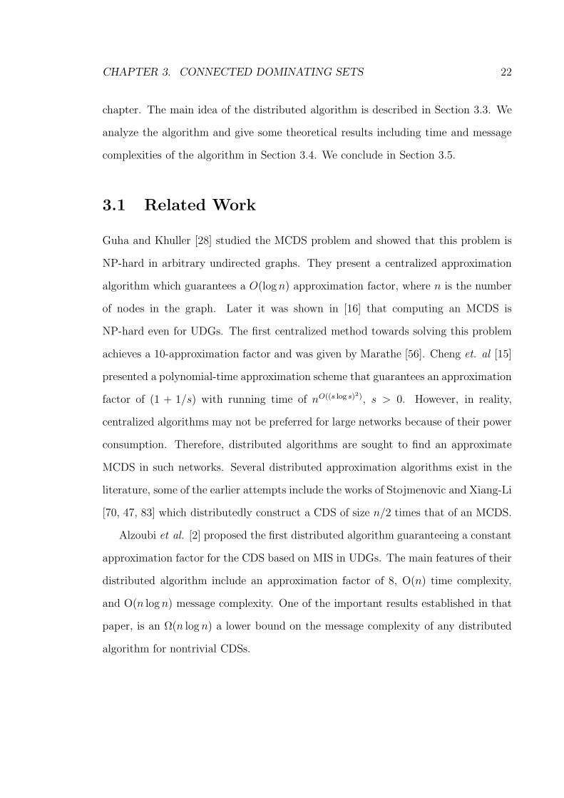
In Figure 3.1, we give a simple example where the black nodes by Phase I of the
algorithm A form a CDS. Node 4 colors itself black since its convex hull CH(N [4]) =
1, 2, 3, 5 (shown in dashed line segments) is not included in any of the convex hulls
CHAPTER 3. CONNECTED DOMINATING SETS 26
CH(N [1]), CH(N [2]), CH(N [3]) or CH(N [5]). For the same reason, nodes 5 and 6
color themselves black. However, nodes 1, 2, 3, 7, 8, and 9 are colored grey because
each of their computed convex hulls is included in its corresponding neighbor’s convex
hull.
1
2 3
4
5 6
7
8
9
Figure 3.1: Node 4 is black since CH(N [4]) = 1, 2, 3, 5 (shown in dashed linesegments) is not included in any of CH(N [1]), CH(N [2]), CH(N [3]) or CH(N [5]).The same applies to nodes 5 and 6.
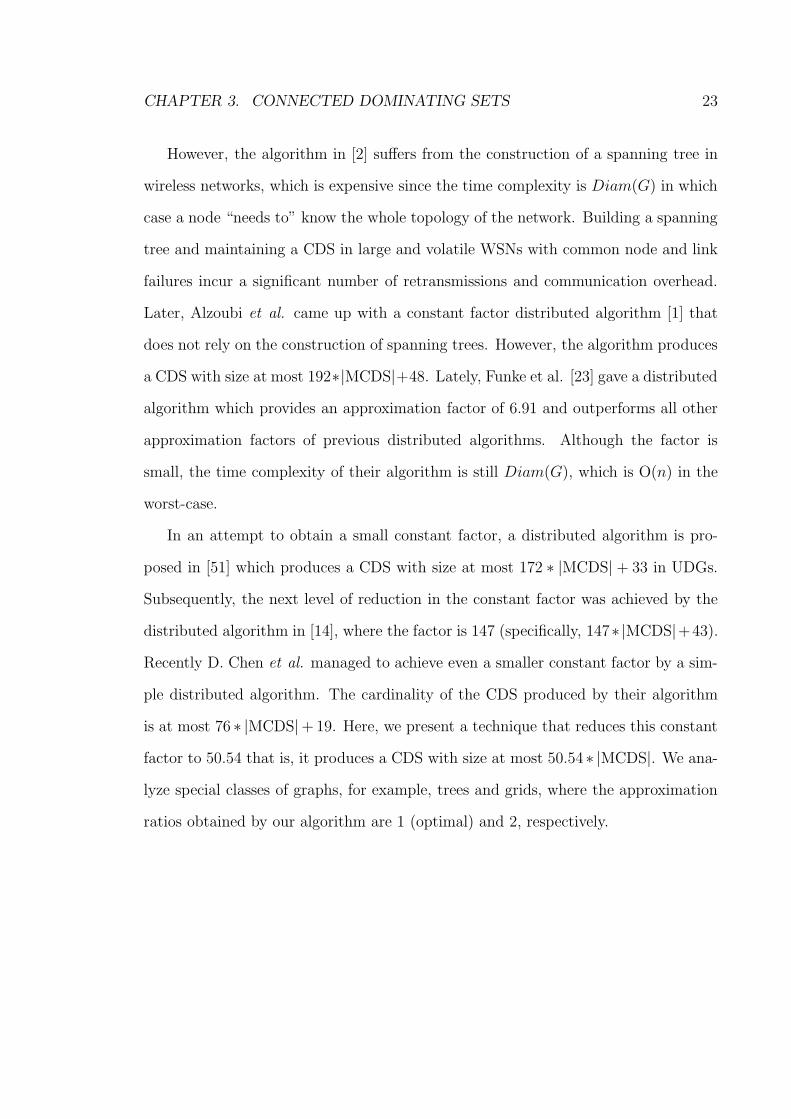
Phase II (Finding an MIS S and a set C of connectors):
This phase begins when Phase I is finished, that is, when there are no white nodes
in G. In this phase, first, as mentioned before an MIS S is constructed from the set
of black nodes B by following the distributed algorithm [66]. The authors in [66]
present a very fast O(log∗ n) distributed algorithm for computing such an MIS for
any growth bounded graph, where the growth boundedness of a graph means that in a
constant neighborhood of any node there is a constant number of independent nodes.
(It can be mentioned that a UDG is a growth bounded graph since for any node u
the number of independent nodes in its r-neighborhood, Nr(u), is O(r2).)
As S is not a dominating set in G, some grey nodes in G may not be dominated
(covered) by S. Note that according to the algorithm, for each grey node u there must

CHAPTER 3. CONNECTED DOMINATING SETS 27
be at least a black neighbor v ∈ N(u) ∩ B such that CH(u) ⊆ CH(v), otherwise u
would not be grey. Let B(u) denote the set of such black neighbors of u.
Now we find an additional set B ′ of nodes from V \S in the following way to make
S∪B′ a dominating set in G. Call the grey nodes not dominated by S orphan nodes.
An orphan node u selects a black node from B(u) to dominate itself. If |B(u)| > 1,
then u selects the one with the minimum id. The set of black nodes selected by all
such grey nodes constitutes the set B ′. Observe that S ∪ B ′ is now a dominating set
in G because all the orphan nodes have at least one neighbor in B ′. Change the color
of the nodes in B \ (S ∪ B ′) into grey.
Although S∪B′ dominates the nodes in G, it is not necessarily connected. There-
fore, a set of connectors C from V \ S is sought to connect the MIS nodes S in order
to find a CDS in G. A node u ∈ S connects to a node v ∈ S, u 6= v with the
minimum id, which is at most 3 hops away. Therefore, at most two intermediate
nodes between u and v are selected to be in C. All such selected intermediate nodes
form the connector set C. The nodes in C color themselves black. Finally, the union
S ∪ B′ ∪ C forms the CDS∗ in G.
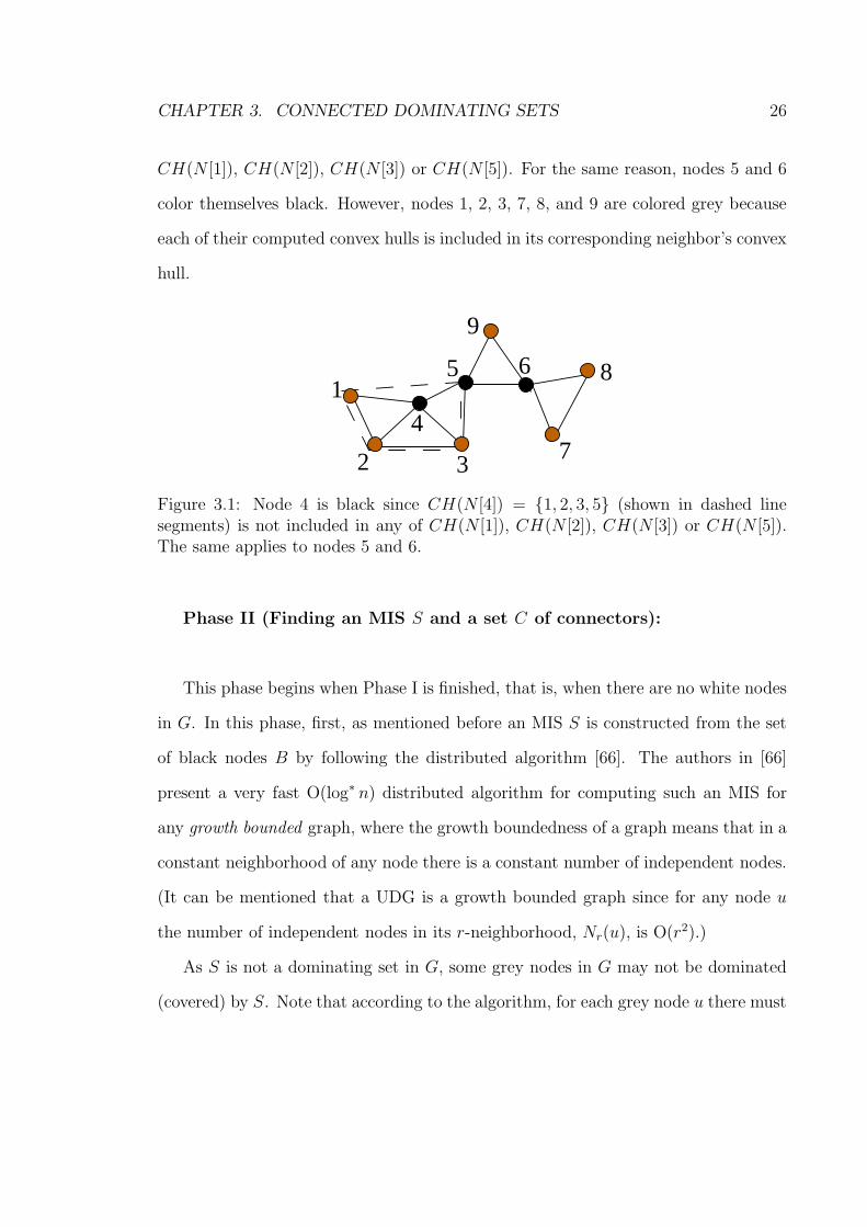
For an illustration, we provide a complete example of Phase I and Phase II of
algorithm A is given in Figure 3.2:
3.4 Algorithm and Analysis
The proposed distributed algorithm is given in Figure 3.3 which is executed at each
node u.
As mentioned before, the first phase of the algorithm is finished when each node
CHAPTER 3. CONNECTED DOMINATING SETS 28
7 8 9 106
3 41 2 5
(a)13
12
11
3 42 5
7 8 9 106(c)
111
13
12
12
3 42 5
7 8 9 106(b)
111
13
Figure 3.2: (a) After Phase I, B = 1, 2, 3, 4, 5, 6, 7, 8, 9, 10. (b) S consists of nodes4, 10. Additional node set is B ′ = 1, 6. (c) After Phase II the solution is S ∪C ∪B′ = 1, 4, 5, 6, 10, where C = 5. The MCDS consists of 1, 6.
is either black or grey. Here we provide a lemma which is essential for the proofs of
other results. This lemma guarantees that the set of black nodes B found through
Phase I is a CDS.
Lemma 3.4.1 The set B forms a CDS in G.
Proof We prove the lemma by contradiction. Suppose u is grey. Then from the
algorithm (consider Phase I only) we derive either Case 1: CH(N [u]) ⊂ CH(N [v])
for some v ∈ N [u]) or Case 2: if such v does not exist, there are some nodes v with
CH(N [u]) = CH(N [v]) and there is a v with id(v) < id(u). In Case 1, if there are
several such nodes with this property, take a node v with the maximal size (in terms
of the number of vertices) CH(N [v]) (using the partial order “subset of or equal”). If
there is still a tie, take the one with the minimum id. Node v cannot be colored grey

CHAPTER 3. CONNECTED DOMINATING SETS 29
Distributed Algorithm for CDSPHASE I:1: If ∃v ∈ N(u) such that CH(N [u]) ⊂ CH(N [v]) Then2: Color u grey Endif3: If @v ∈ N(u) such that CH(N [u]) ⊂ CH(N [v]) Then4: Color u black Endif5: If ∃v ∈ N(u) such that CH(N [u]) = CH(N [v]) Then6: If id(u) < id(v), ∀v ∈ N(u) Then7: Color u black8: Else9: Color u grey10: Endif EndifPHASE II:11: If u is black Then Run MIS [66] Endif12: If u is grey Then Select a node in B(u) Endif13: If u is in S Then Select connectors between u and v Endif// v ∈ S is at most 3 hops away and id(u) > id(v)
Figure 3.3: A Distributed algorithm for the CDS problem.
at the beginning of the algorithm since this would mean the presence of a node w,
where w ∈ N(u) and CH(N [u]) ⊂ CH(N [v]) ⊂ CH(N [w]) implying that CH(N [v])
is not maximal. Also it can not be colored grey in the next step since that implies
that there is a node w with CH(N [u]) ⊂ CH(N [v]) = CH(N [w]) and id(w) < id(v),
so v does not have the minimum id. Therefore, v is colored black.
Of all such nodes (v) with the property of Case 2, take the one with the minimum
id. Node v is not colored grey at the beginning of the algorithm, since this would imply
the presence of a node w with CH(N [u]) = CH(N [v]) ⊂ CH(N [w]) and w ∈ N(v).
However, it will be colored black in the next step but this is a contradiction. So B is
a dominating set.
In order to prove that the node set B is connected, we show that there is a
path between any two nodes u, v ∈ B containing only black nodes. For the sake
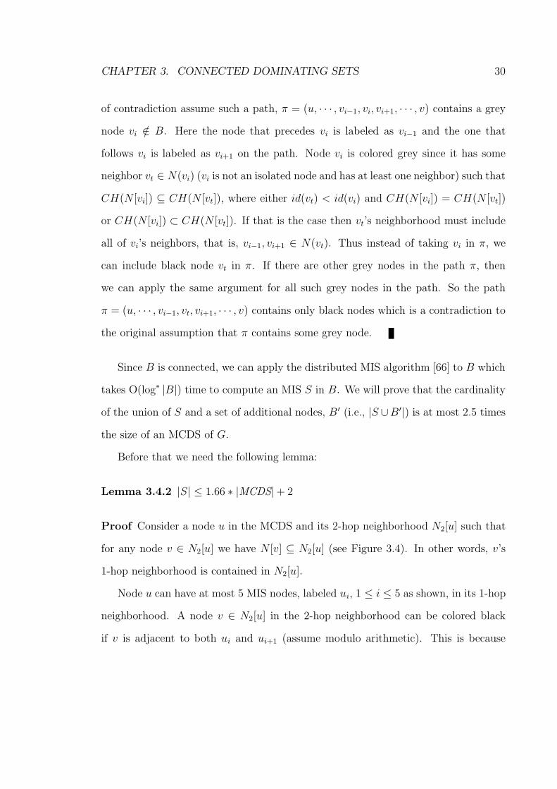
CHAPTER 3. CONNECTED DOMINATING SETS 30
of contradiction assume such a path, π = (u, · · · , vi−1, vi, vi+1, · · · , v) contains a grey
node vi /∈ B. Here the node that precedes vi is labeled as vi−1 and the one that
follows vi is labeled as vi+1 on the path. Node vi is colored grey since it has some
neighbor vt ∈ N(vi) (vi is not an isolated node and has at least one neighbor) such that
CH(N [vi]) ⊆ CH(N [vt]), where either id(vt) < id(vi) and CH(N [vi]) = CH(N [vt])
or CH(N [vi]) ⊂ CH(N [vt]). If that is the case then vt’s neighborhood must include
all of vi’s neighbors, that is, vi−1, vi+1 ∈ N(vt). Thus instead of taking vi in π, we
can include black node vt in π. If there are other grey nodes in the path π, then
we can apply the same argument for all such grey nodes in the path. So the path
π = (u, · · · , vi−1, vt, vi+1, · · · , v) contains only black nodes which is a contradiction to
the original assumption that π contains some grey node.
Since B is connected, we can apply the distributed MIS algorithm [66] to B which
takes O(log∗ |B|) time to compute an MIS S in B. We will prove that the cardinality
of the union of S and a set of additional nodes, B ′ (i.e., |S ∪B′|) is at most 2.5 times
the size of an MCDS of G.
Before that we need the following lemma:
Lemma 3.4.2 |S| ≤ 1.66 ∗ |MCDS| + 2
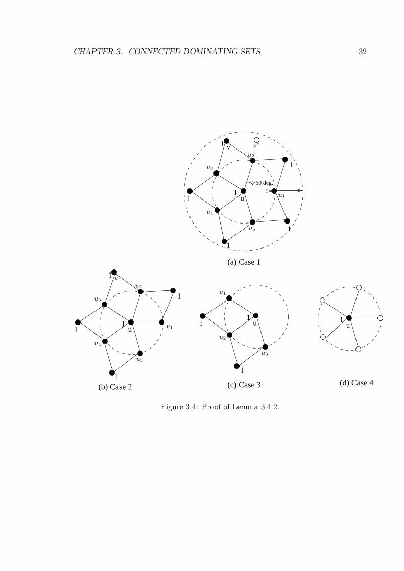
Proof Consider a node u in the MCDS and its 2-hop neighborhood N2[u] such that
for any node v ∈ N2[u] we have N [v] ⊆ N2[u] (see Figure 3.4). In other words, v’s
1-hop neighborhood is contained in N2[u].
Node u can have at most 5 MIS nodes, labeled ui, 1 ≤ i ≤ 5 as shown, in its 1-hop
neighborhood. A node v ∈ N2[u] in the 2-hop neighborhood can be colored black
if v is adjacent to both ui and ui+1 (assume modulo arithmetic). This is because

CHAPTER 3. CONNECTED DOMINATING SETS 31
v’s convex hull CH(N [v]) will not be included in any of its neighbors’ convex hulls.
Similarly, any node v∗ which is 2-hop away from u and not adjacent to both ui and
ui+1 will not be colored black since CH(N [v∗]) must be included in the convex hull
CH(N [u∗]) of some node u∗ ∈ N [u].
According to the above arrangement of the nodes we can have at most 11 black
nodes in N2[u]. As we apply an MIS algorithm, we can have at most six MIS nodes
in N2[u] (the MIS nodes are labeled ‘1’ in the figure).
Now we determine the minimum number of MCDS nodes that u must have in
N [u] in order to cover all the MIS nodes in N2[u]. In order to do that we need to
investigate the following four cases:
Case 1: At least four MCDS nodes, namely, u, ui, ui+2 and ui+3 are required to
cover (dominate) at most six MIS nodes (Figure 3.4(a)).
Case 2: At least three MCDS nodes (u, ui, ui+2) are required to cover at most
five MIS nodes (Figure 3.4(b)).
Case 3: At least two MCDS nodes (u, ui) are required to cover at most three
MIS nodes (Figure 3.4(c)).
Case 4: At least one MCDS node (u) is required to cover one MIS node (Figure
3.4(d)).
Analyzing the above relations we have the following:
Thus |S| ≤ 5 ∗ d |MCDS|3
e ≤ d1.66 ∗ |MCDS|e + 1 ≤ 1.66 ∗ |MCDS| + 2. This
completes our proof.
Theorem 3.4.3 Let B be a CDS in G and S be any MIS in B. If B ′ denotes the
set of additional nodes, then |S ∪ B ′| ≤ 2.66 ∗ |MCDS| + 2.
Proof Recall that for any orphan node u (u is grey) there must be at least a black
CHAPTER 3. CONNECTED DOMINATING SETS 32
11
u
1
1
1
1
1u
1
>60 deg.
v
1u
1
1
1
1
1
1u
v
(b) Case 2 (c) Case 3 (d) Case 4
(a) Case 1
u1
u2
u3
u2
u3
u4
u5
v∗
u1
u2
u3
u4
u5
u1
Figure 3.4: Proof of Lemma 3.4.2.
CHAPTER 3. CONNECTED DOMINATING SETS 33
node v ∈ N(u) such that CH(N(u)) ⊆ CH(N(v)), otherwise u would not be grey. In
order for the MCDS to cover u, either u must belong to an MCDS or there will be at
least a node v′ ∈ MCDS∩N(u). In any case an MCDS must have at least one node
from N [u]. Since u selects the node with the minimum id from N(u), the number of
nodes in MCDS will not be greater than the number of nodes selected by all orphan
nodes in the graph. Therefore, |B ′| ≤ |MCDS|, where B′ is the set of nodes selected
by all orphan nodes in the graph.
Therefore, combining the results from Lemma 3.4.2 we obtain the following, |S ∪
B′| ≤ 2.66 ∗ |MCDS| + 2.
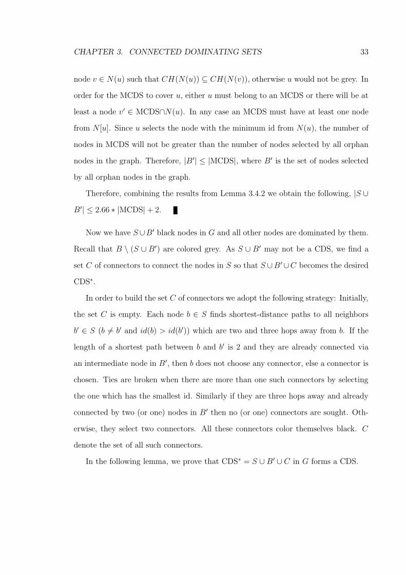
Now we have S∪B ′ black nodes in G and all other nodes are dominated by them.
Recall that B \ (S ∪ B ′) are colored grey. As S ∪ B ′ may not be a CDS, we find a
set C of connectors to connect the nodes in S so that S ∪B ′ ∪C becomes the desired
CDS∗.
In order to build the set C of connectors we adopt the following strategy: Initially,
the set C is empty. Each node b ∈ S finds shortest-distance paths to all neighbors
b′ ∈ S (b 6= b′ and id(b) > id(b′)) which are two and three hops away from b. If the
length of a shortest path between b and b′ is 2 and they are already connected via
an intermediate node in B ′, then b does not choose any connector, else a connector is
chosen. Ties are broken when there are more than one such connectors by selecting
the one which has the smallest id. Similarly if they are three hops away and already
connected by two (or one) nodes in B ′ then no (or one) connectors are sought. Oth-
erwise, they select two connectors. All these connectors color themselves black. C
denote the set of all such connectors.
In the following lemma, we prove that CDS∗ = S ∪ B′ ∪ C in G forms a CDS.
CHAPTER 3. CONNECTED DOMINATING SETS 34
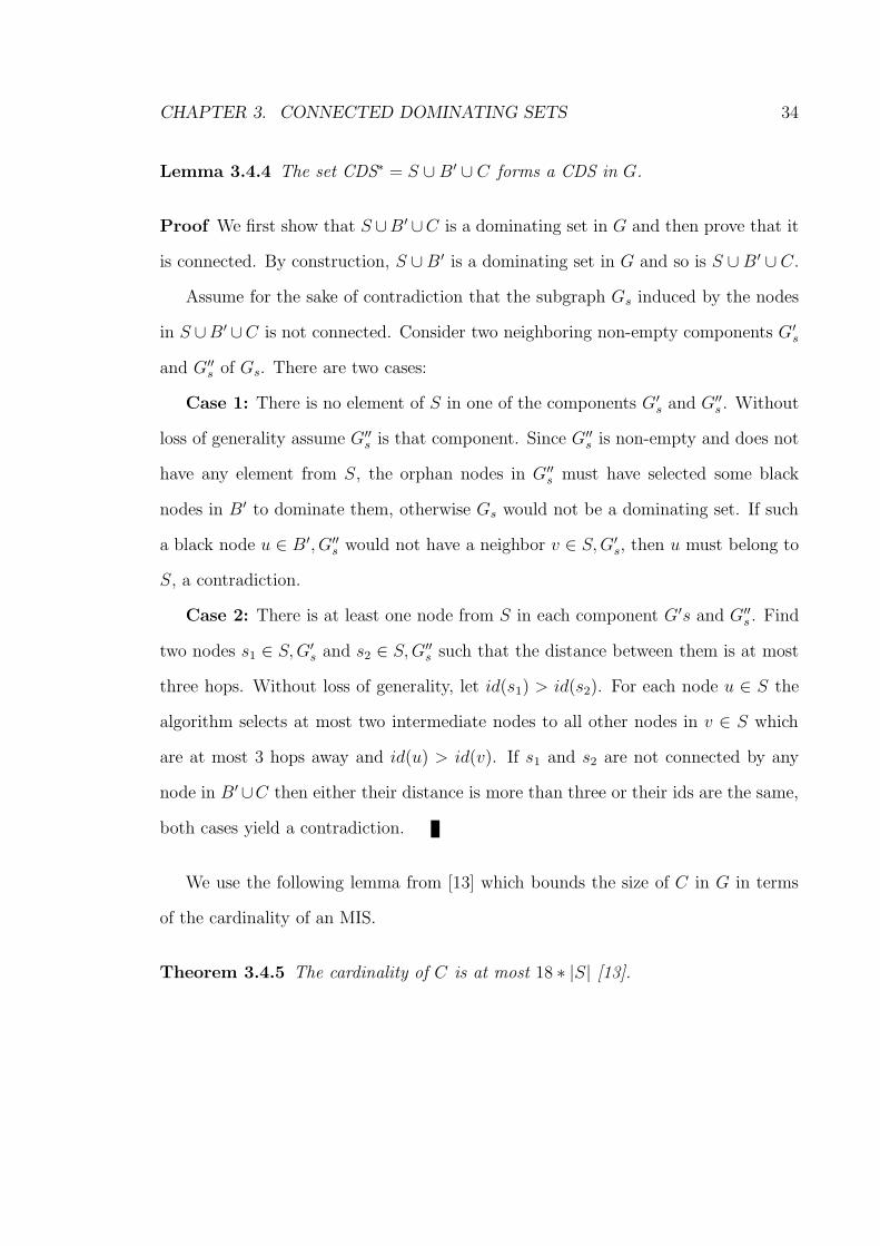
Lemma 3.4.4 The set CDS∗ = S ∪ B′ ∪ C forms a CDS in G.
Proof We first show that S ∪B ′ ∪C is a dominating set in G and then prove that it
is connected. By construction, S ∪ B ′ is a dominating set in G and so is S ∪ B ′ ∪ C.
Assume for the sake of contradiction that the subgraph Gs induced by the nodes
in S ∪B′ ∪C is not connected. Consider two neighboring non-empty components G′s
and G′′s of Gs. There are two cases:
Case 1: There is no element of S in one of the components G′s and G′′
s . Without
loss of generality assume G′′s is that component. Since G′′
s is non-empty and does not
have any element from S, the orphan nodes in G′′s must have selected some black
nodes in B′ to dominate them, otherwise Gs would not be a dominating set. If such
a black node u ∈ B′, G′′s would not have a neighbor v ∈ S, G′
s, then u must belong to
S, a contradiction.
Case 2: There is at least one node from S in each component G′s and G′′s . Find
two nodes s1 ∈ S, G′s and s2 ∈ S, G′′
s such that the distance between them is at most
three hops. Without loss of generality, let id(s1) > id(s2). For each node u ∈ S the
algorithm selects at most two intermediate nodes to all other nodes in v ∈ S which
are at most 3 hops away and id(u) > id(v). If s1 and s2 are not connected by any
node in B′∪C then either their distance is more than three or their ids are the same,
both cases yield a contradiction.
We use the following lemma from [13] which bounds the size of C in G in terms
of the cardinality of an MIS.
Theorem 3.4.5 The cardinality of C is at most 18 ∗ |S| [13].

CHAPTER 3. CONNECTED DOMINATING SETS 35
Theorem 3.4.6 For any maximal independent set S in B, a set B ′ of additional
nodes and a set C of connectors in a UDG G = (V, E), we have |S ∪ B ′ ∪ C| ≤
50.54 ∗ |MCDS| + 38.
Proof Combining the results of Theorems 3.4.3 and 3.4.5 we get:
|C| ≤ 18 ∗ |S|
≤ 18 ∗ |S ∪ B′|
≤ 18 ∗ 2.66 ∗ |MCDS| + 36
= 47.88 ∗ |MCDS| + 36.
Then,
|S ∪ B′ ∪ C| ≤ |S ∪ B′| + |C|
≤ 2.66 ∗ |MCDS| + 2 + 47.88 ∗ |MCDS| + 36
= 50.54 ∗ |MCDS| + 38.
One feature of our algorithm A is that it guarantees an MCDS (minimum CDS)
for trees. The interesting thing is that we do not need to check whether G is a tree to
compute an MCDS. This means that if G is a tree, algorithm A generates the optimal
CDS. Other algorithms such as [3] require G to be checked for being a tree in order to
construct a CDS. That is, the problem with their algorithm is that the nodes need to
construct a spanning tree from the underlying graph which is an expensive operation
in terms of energy usage.
We prove the optimality result in the following theorem.
CHAPTER 3. CONNECTED DOMINATING SETS 36
Theorem 3.4.7 If the underlying unit disk graph G is a tree with |V | > 2 algorithm
A produces an MCDS.
Proof It is well known that for a tree an MCDS consists only of the internal nodes
of the tree. We prove the theorem by contradiction. Suppose a CDS produced by
algorithm A consists of some leaves of the tree. Let ` be such a leaf and p its parent.
Since ` is in the CDS, its computed convex hull CH(N [`]) is not included in any of
its neighbor’s convex hull and its color is black. However, its only neighbor is p and
p’s neighborhood contains at least two neighbors including `, otherwise p is a leaf.
Obviously, the convex hull CH(N [`]) is included in CH(N [p]), since N [`] includes
only ` and p. So ` would be colored grey and cannot be in the CDS, which is a
contradiction.
We analyze the performance of our algorithm in grids where we show that the
cardinality of the CDS produced by algorithm A is less than twice the size of an
MCDS.
Theorem 3.4.8 Given a m×n grid, where nodes are placed at the intersection points
and the Euclidean distance between two adjacent nodes equals 1, algorithm A produces
a CDS such that |CDS∗| ≤ 2 ∗ |MCDS|.
Proof By analyzing the m × n grid, the size of the minimum connected dominating
set can be calculated as: |MCDS| = m−12
∗ n + m−12
− 1 = mn−n+m−32
, when m is odd
and |MCDS| = m2∗ n + m
2− 1 = mn+m−2
2, when m is even. The cardinality of the
CDS generated by algorithm A is mn. Thus if m is even the approximation factor
is 2 × mnmn+m−2
< 2. However, if m is odd and m > n, the approximation factor is
2 × mnmn−n+m−3
< 2.

CHAPTER 3. CONNECTED DOMINATING SETS 37
Corollary 3.4.9 For any induced subset of an m × n grid, algorithm A produces a
CDS with at most twice as many nodes as an MCDS.
3.4.1 Time and Message Complexities
According to our model LOCALS, the time complexity of algorithm A is derived as
follows. Each node u receives the location information of its neighbors and sends
its location to them which can be done in a single round. Then u computes the
convex hull CH(N [u]) and checks whether the convex hull is included in any of the
convex hulls of its neighbors. However, the whole process of computing and compar-
ing CH(N [u]) with CH(N [v]), ∀v ∈ N(u), for inclusion is negligible in synchronous
systems [61], where the time complexity is measured in terms of number of rounds.
After computing CH(N [u]), u sends the list of vertices of CH(N [u]) to all its neigh-
bors and receives theirs’ as well. Since the message size is arbitrary, the exchange of
convex hulls can be done in a single round. The computation of the distributed MIS
[66] takes O(log∗ |B|) time, where B is the set of black nodes. The distributed MIS
algorithm in B generates the set S. Each node in S finds at most two intermediate
nodes in S which are at most three hops away from it. However, the number of
such neighbors is a constant [72] for a node u ∈ S. Thus computing such shortest
paths takes O(1)-time. Therefore, the overall time complexity of the algorithm is
O(log∗ |B|)=O(log∗ n).
To compute the message complexity, we see that each node has to send its location,
id (all these can be packed in a single message) to its neighbors, which takes O(n)
messages to be sent. Again, after computing the convex hull CH(N [u]), node u sends
CH(N [u]) (the nodes in the convex hull are put in a message) to its neighbors which
CHAPTER 3. CONNECTED DOMINATING SETS 38
also takes O(n) messages to be exchanged in the network. However, to compute an
MIS it takes O(|E| ∗ log∗ n) [66] messages. Thus the message complexity of the entire
algorithm is O(|E| ∗ log∗ n).
3.5 Conclusion
Computing a CDS distributedly in WSNs is a very well studied problem. However,
devising distributed algorithms for constructing such CDSs become more challenging
when it is aimed to obtain a small constant approximation factor with each node
knowing a limited amount of information about the topology of the underlying net-
work. Several distributed algorithms are known in this context and interestingly
almost all of them use the same approach: find an MIS in the network graph and
then connect them through other nodes to construct the set.
Instead of finding an MIS in the whole network, our approach first builds a con-
nected subgraph in the network graph, then finds an MIS in the subgraph and finally
connects the nodes in the MIS through other nodes. By this technique, we could re-
move a number of unwanted nodes from being in the connected dominating set. This
way our simple distributed algorithm guarantees a relatively small constant approxi-
mation factor which is a good improvement over the best known constant factor [13].
The main difficulty in lowering the constant factor lies in the reduction of the size
of the connectors used to connect the nodes in the MIS. Exploring further geometric
properties of unit disk graphs may help achieve a better bound for the size of the set
of connector nodes. In future work, we look forward to finding distributed constant
factor CDS algorithms in special classes of graphs, such as for example, planar graphs.

Chapter 4
Family of Connected Dominating
Sets
In the last chapter, we studied the problem of constructing a single CDS in WSNs.
However finding a CDS (even the MCDS) and using it all the time can exhaust the
energy of the nodes of the CDS faster than other nodes in the network. Therefore,
devising strategies to obtain a number of different CDSs and employing them one by
one is a challenging task in the context of WSNs.
In this chapter, we investigate the problem of computing a family of connected
dominating sets in a WSN in a distributed manner. We present a distributed al-
gorithm that computes a family S1, S2, · · · , Sm of non-trivial CDSs with the goal to
maximize α = m/k, where k=maxu∈V |i : u ∈ Si|. In other words, we wish to find
as many CDSs as possible while minimizing the number of frequencies of each node
in these sets. Since CDSs play an important role for maximizing network lifetime
when they are used as backbones for broadcasting messages, maximizing α reduces
39

CHAPTER 4. FAMILY OF CONNECTED DOMINATING SETS 40
the possibility of repeatedly using the same subset of nodes as backbones. We pro-
vide an upper bound on the value of α via a ‘nice’ relationship between all minimum
vertex-cuts and CDSs in the network graph and present a distributed algorithm for
the α maximization problem. For a subclass of UDGs, it is shown that our algorithm
achieves a constant approximation factor of the optimal solution. As before a WSN
is modelled as a UDG.
4.1 A Motivating Example
We are motivated by an important observation for the general CDS construction
in WSNs where the main goal is to obtain a “small” approximation factor for the
computed CDS, since finding a minimum cardinality CDS is NP-hard [16]. Consider
the wheel graph in Figure 4.1 (a) with 9 nodes. Assume that each node has 9 units of
energy and each transmission for a unit of data from a node to its neighbor consumes
one unit of energy, neglecting the consumption of energy for message reception. The
optimal CDS contains only node 9 at the center.
Suppose each border node 1, 2, · · · , 8 has a unit of data to be broadcast via
the center node 9 in each communication round. That is, whenever a node on the
periphery sends a message, it is node 9 which broadcasts (relays) it and all other
nodes receive the message. After eight rounds corresponding to eight border nodes
transmitting their data through the center node, the center node will be left with
1 unit of energy while all the border nodes still contain eight units of energy each.
After the 9th round, node 9 will have completely exhausted its energy and the other
nodes will have 8 units of energy each for continuing operation. Thus finding an
optimal solution might not always be helpful in scenarios like this and it is not hard

CHAPTER 4. FAMILY OF CONNECTED DOMINATING SETS 41
to construct a family of such examples.
One easy way to get around this problem is to devise algorithms that can in some
way evenly distribute the energy consumption among the nodes in the network by not
using the same subset of nodes for all broadcasting operations. Clearly this may not
yield a ‘small-sized’ or constant factor approximation solution to the CDS problem but
can be used to prolong the lifetime of the network which depends on the functioning
of every node in the network. Using node 9 as a CDS for one broadcasting operation
then leaving it free and engaging six consecutive nodes from the border nodes as
next CDSs for successive rounds (See Figure 4.1(b), (c)) for each broadcasting clearly
enhances the overall network lifetime. In other words, we have two scenarios. First,
we can use only the middle node as the CDS which gives m/k = 1, where m is the
number of CDSs generated and k is the maximum number of occurrences of a node
in these CDSs. In the second scenario, we can use 3 CDSs, where the nodes are taken
from the border nodes only and one CDS containing only the middle node. Thus we
get m/k = 4/3 which means that if the network is used for 4 rounds, for the first
scenario, the middle node is used for 4 rounds, and in the second scenario, no node
is used for more than 3 rounds.
In general, the above problem may be solved by finding a large number of disjoint
connected dominating sets since doing so has a direct impact on conserving the energy
of individual sensors and hence prolonging the network lifetime. However, as we will
show, it is not always possible to find a large number of such disjoint sets because
the number of disjoint CDSs is bounded by the size of a minimum vertex-cut of the
graph. Thus, the main focus is to find as many CDSs as possible while minimizing the
frequency of participations of each node in the network. In other words, we would like
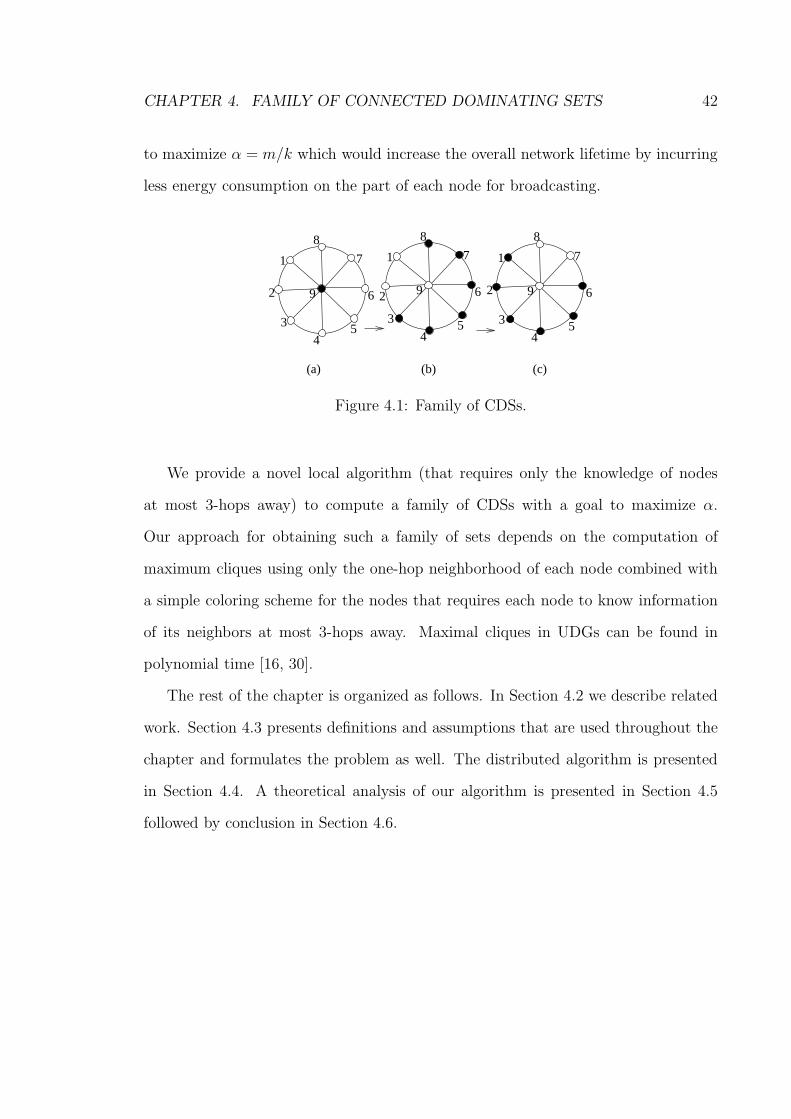
CHAPTER 4. FAMILY OF CONNECTED DOMINATING SETS 42
to maximize α = m/k which would increase the overall network lifetime by incurring
less energy consumption on the part of each node for broadcasting.
2
1
3
45
6
7
8
9 2
8
1
3
45
6
7
9 2
1
3
45
6
7
9
8
(a) (b) (c)
Figure 4.1: Family of CDSs.
We provide a novel local algorithm (that requires only the knowledge of nodes
at most 3-hops away) to compute a family of CDSs with a goal to maximize α.
Our approach for obtaining such a family of sets depends on the computation of
maximum cliques using only the one-hop neighborhood of each node combined with
a simple coloring scheme for the nodes that requires each node to know information
of its neighbors at most 3-hops away. Maximal cliques in UDGs can be found in
polynomial time [16, 30].
The rest of the chapter is organized as follows. In Section 4.2 we describe related
work. Section 4.3 presents definitions and assumptions that are used throughout the
chapter and formulates the problem as well. The distributed algorithm is presented
in Section 4.4. A theoretical analysis of our algorithm is presented in Section 4.5
followed by conclusion in Section 4.6.

CHAPTER 4. FAMILY OF CONNECTED DOMINATING SETS 43
4.2 Related Work
There is a large body of literature [2, 3, 15, 23, 28, 56, 70, 47] regarding finding an
MCDS in WSNs which focuses on the construction of a single CDS and the effort
is to devise algorithms to produce a small approximation factor for it. Aside from
looking for a single CDS with a small approximation factor, there has been some
research towards finding a family of dominating sets [58, 62, 21, 69] for data gath-
ering and sensing operations in sensor networks. In [21], the authors consider the
problem of finding a maximum number of disjoint dominating sets called the domatic
partition (we study this problem in the next chapter). They show that every graph
with maximum degree 4 and minimum degree δ contains a domatic partition of size
(1 − o(1))(δ + 1)/ln 4. They provide a centralized algorithm to produce a domatic
partition of size Ω(δ/ln4).
The papers [62, 58, 69] are somewhat related to ours since they investigate the
problem of maximizing the lifetime of wireless networks by generating disjoint domi-
nating sets (not connected dominating sets) for data gathering purposes. The general
focus is that the nodes in the dominating set act as “coordinators” for the network
and the rest of the nodes remain in an energy-efficient sleep mode. Thus to maximize
the lifetime of the network, it is important to rotate the coordinatorship among the
nodes in the network so that every node is roughly given an equal opportunity to go
into sleep mode.
In particular, the authors in [69] propose a centralized algorithm, without provid-
ing any worst case analysis or bound, to generate a number of disjoint dominating
sets in order to cover a geometrical region by network nodes for as long as possible.
A general version of the domatic partition called k-domatic partition (k ≥ 2), where

CHAPTER 4. FAMILY OF CONNECTED DOMINATING SETS 44
in each dominating set a node is dominated by at least k nodes, is considered in [62].
Their algorithms construct a k− domatic partition of size at least a constant fraction
of the largest possible (k − 1)-domatic partition.
In [58], the authors look at a variant of the above problem and propose a random-
ized algorithm for maximizing the network lifetime. The problem considered in [58]
is called the Maximum Cluster-Lifetime problem, where they aim to find an optimal
schedule consisting of a set of pairs (D1, t1), · · · , (Dk, tk), where Di is a dominating set
and ti is the time during which Di is active. The problem then asks for the schedule S
with maximum length L(S) such that∑
i:v∈Diti ≤ bv, where bv is the maximum time
that v can be in a dominating set. The randomized algorithm computes a schedule
which is an O(log n)-approximation algorithm with high probability.
4.3 Preliminaries and Problem Formulation
Each node u has an ordered triple, (ct(u), deg(u), id(u)), where the first element ct(u)
denotes the number of times u has already participated in previous CDSs, deg(u) and
id(u) denote the degree and id of u. Initially, ct(u) = 0, ∀u ∈ V , and this is updated
as the algorithm is executed. For a maximum clique X ⊆ N [u] and u, v ∈ X,
we say node u is lexicographically smaller than node v if (ct(u), deg(u), id(u)) <
(ct(v), deg(v), id(v)), i.e., either ct(u) < ct(v) or ct(u) = ct(v) and deg(u) < deg(v)
or ct(u) = ct(v) and deg(u) = deg(v) and id(u) < id(v). The rank of node u with
respect to clique X denoted by r(X(u)) is the index of the lexicographically sorted
(ascending order) triples of the nodes of X. Note that the rank r(X(u)) is changed
by the update of the variable ct(u).

CHAPTER 4. FAMILY OF CONNECTED DOMINATING SETS 45
4.3.1 Problem Formulation
Given a UDG G = (V, E), we would like to find a family of subsets S1, S2, · · · , Sm
such that
i) ∀i, Si is a CDS
ii) and α = m/k is maximized, where k=maxu∈V |i : u ∈ Si|.
4.4 A 3-local CDS Algorithm
We provide a local algorithm for generating a family of CDSs. The algorithm uses a
simple coloring scheme where initially all nodes are white and when a node becomes
a member of the CDS Si, it becomes black. Set Si, whose members are all black,
becomes the virtual backbone and remains active for a time-slot (consisting of fixed
units of time) to perform broadcasting. After the time-slot, all black nodes change
their color into white. Then the algorithm (part of it) is executed again and a new
set Si+1 of black nodes is formed which remains active for another time-slot and so
on. In this section, we present a simple algorithm for computing a family of CDSs in
G which is based on coloring the nodes of G. This algorithm appears in [39]. Here
we outline the algorithm which consists of two phases described in what follows.
4.4.1 Dominating Set Generation: Phase I
In Phase I, each node u computes a maximum clique in N [u] following the polynomial
time algorithm [30] which computes maximum cliques in UDGs. Let C(u) denote the
maximum clique computed by u. Henceforth maximum cliques are just called cliques
unless otherwise stated. Node u sends the nodes in C(u) to all its direct neighbors v
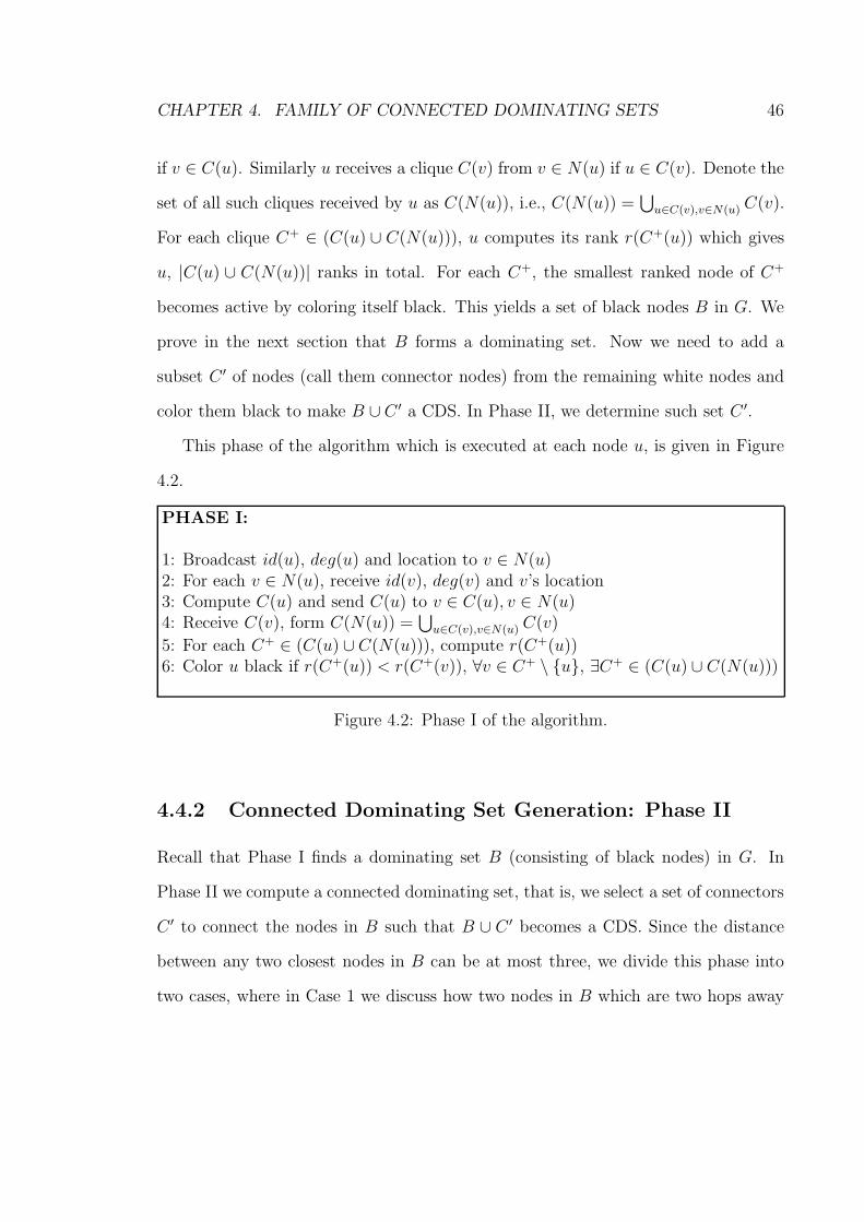
CHAPTER 4. FAMILY OF CONNECTED DOMINATING SETS 46
if v ∈ C(u). Similarly u receives a clique C(v) from v ∈ N(u) if u ∈ C(v). Denote the
set of all such cliques received by u as C(N(u)), i.e., C(N(u)) =⋃
u∈C(v),v∈N(u) C(v).
For each clique C+ ∈ (C(u) ∪ C(N(u))), u computes its rank r(C+(u)) which gives
u, |C(u) ∪ C(N(u))| ranks in total. For each C+, the smallest ranked node of C+
becomes active by coloring itself black. This yields a set of black nodes B in G. We
prove in the next section that B forms a dominating set. Now we need to add a
subset C ′ of nodes (call them connector nodes) from the remaining white nodes and
color them black to make B ∪ C ′ a CDS. In Phase II, we determine such set C ′.
This phase of the algorithm which is executed at each node u, is given in Figure
4.2.
PHASE I:
1: Broadcast id(u), deg(u) and location to v ∈ N(u)2: For each v ∈ N(u), receive id(v), deg(v) and v’s location3: Compute C(u) and send C(u) to v ∈ C(u), v ∈ N(u)4: Receive C(v), form C(N(u)) =
⋃u∈C(v),v∈N(u) C(v)
5: For each C+ ∈ (C(u) ∪ C(N(u))), compute r(C+(u))6: Color u black if r(C+(u)) < r(C+(v)), ∀v ∈ C+ \ u, ∃C+ ∈ (C(u) ∪ C(N(u)))
Figure 4.2: Phase I of the algorithm.
4.4.2 Connected Dominating Set Generation: Phase II
Recall that Phase I finds a dominating set B (consisting of black nodes) in G. In
Phase II we compute a connected dominating set, that is, we select a set of connectors
C ′ to connect the nodes in B such that B ∪ C ′ becomes a CDS. Since the distance
between any two closest nodes in B can be at most three, we divide this phase into
two cases, where in Case 1 we discuss how two nodes in B which are two hops away

CHAPTER 4. FAMILY OF CONNECTED DOMINATING SETS 47
from each other connect themselves via connectors. Case 2 is the same but such nodes
are exactly three hops away from each other.
Case 1: Consider a node u ∈ B. Node u selects a connector node for each node
v ∈ B, exactly two hops away from it and id(u) > id(v), if there does not exist any
black node w ∈ N(u) ∩ N(v). If there are multiple candidates for such a connector,
the lexicographically smallest one is chosen. Node u send a ‘YES’ message to the
selected connector (denote the connector node c) to turn itself into black.
Case 2: In this case u selects at most two connectors to connect a node v ∈ B
which are exactly three hops away from it and id(u) > id(v). If there already exists
two intermediate black nodes (belonging to B) between u and v, then u does nothing.
Otherwise, the three-hop shortest paths between u and v must contain either one
black node or no black nodes. In the first situation the lexicographically smallest
black node is chosen among all such black nodes. After selecting the black node a
white connector c is selected. Similarly, if there is no black node between u and v,
then u selects two connectors c′, c′′ such that the average ct(.) values of c′ and c′′ (that
is, (ct(c′) + ct(c′′))/2) is smallest (ties are broken arbitrarily). Node u then sends a
‘YES’ message to all such connectors (c or c′ and c′′) it thus selects. After receiving
a ‘YES’ message, connectors turn themselves into black.
Thus the executions of Phases I and II form a CDS Si which consists of black
nodes and these nodes remain active for a certain amount of time (a time-slot) for
broadcasting while the white nodes stay in the energy-efficient sleep mode. Phase II
is given in Figure 4.3. After serving for a time-slot, all nodes in the CDS, i.e., black
nodes, update their ct(.) values by one, send the updated values to their neighbors and
change color into white. All nodes in G then start executing from Line 5 Phase I and

CHAPTER 4. FAMILY OF CONNECTED DOMINATING SETS 48
PHASE II:1: If u is black Then2: If v ∈ B and v is two-hop away from u and id(u) > id(v)3: Find at most a connector c //(lexicographically smallest)4: Send a ‘YES’ message to c //(if there exists such a c)5: Endif6: If v ∈ B and v 3-hop away from u and id(u) > id(v) Then7: Find at most two connectors (c′ or c′′)8: Send a ‘YES’ message to c′ and c′′ //(if there exist such connectors)9: Endif10: Endif11: If u is white and receives a ‘YES’ message Then12: Color u black //(u is a connector)13: Endif14: If u is black Then15: Remain active for a round (black nodes form the current CDS)16: Send ct(u) = ct(u) + 1 to N(u)17: Turn u white //(Just before the next round, turn every node white)18: Endif
Figure 4.3: Phase II of the algorithm.
then Phase II with their updated triples. This generates a new CDS Si+1 consisting
of black nodes, which remains active for another time-slot. Then ct(.) values are
updated and a new CDS Si+2 is constructed, and so on.
Figure 4.4 illustrates the construction of a CDS by coloring certain nodes black.
The numbering of nodes denotes the id of the corresponding nodes and the number
inside the bracket indicates the nodes’ ct(.) values. Initially all ct(.) values are set to
zero and they are incremented by one each time the respective nodes participate in
the CDS. In this example we can construct six different CDSs.
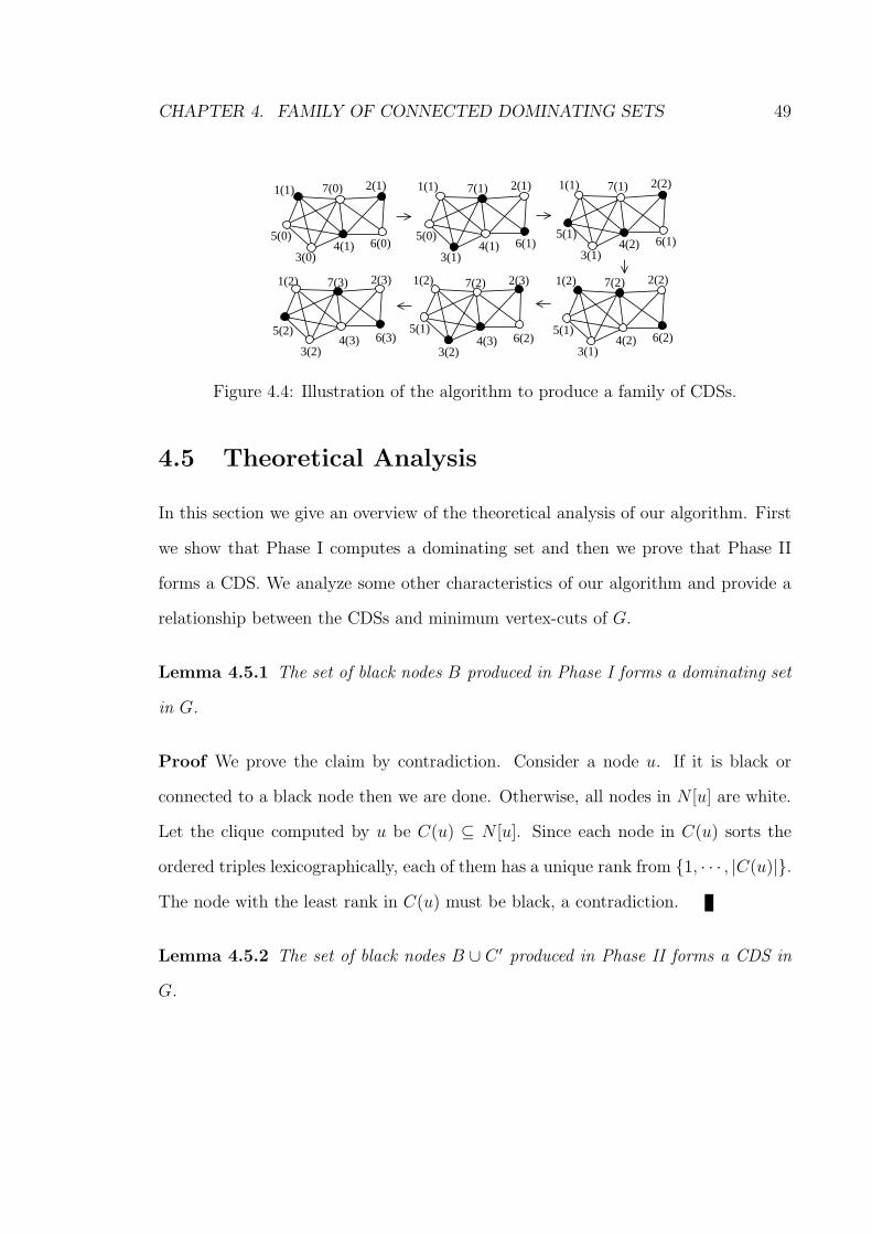
CHAPTER 4. FAMILY OF CONNECTED DOMINATING SETS 49
3(0)4(1) 6(0)
5(0)
1(1) 7(0) 2(1)
3(1)4(2) 6(2)
5(1)
7(2) 2(2)
3(2)4(3) 6(2)
7(2) 2(3)
3(2)4(3) 6(3)
7(3) 2(3)1(2) 1(2) 1(2)
5(2) 5(1)
3(1)4(1) 6(1)
5(0)
7(1) 2(1)
3(1)4(2) 6(1)
5(1)
7(1) 2(2)1(1)1(1)
Figure 4.4: Illustration of the algorithm to produce a family of CDSs.
4.5 Theoretical Analysis
In this section we give an overview of the theoretical analysis of our algorithm. First
we show that Phase I computes a dominating set and then we prove that Phase II
forms a CDS. We analyze some other characteristics of our algorithm and provide a
relationship between the CDSs and minimum vertex-cuts of G.
Lemma 4.5.1 The set of black nodes B produced in Phase I forms a dominating set
in G.
Proof We prove the claim by contradiction. Consider a node u. If it is black or
connected to a black node then we are done. Otherwise, all nodes in N [u] are white.
Let the clique computed by u be C(u) ⊆ N [u]. Since each node in C(u) sorts the
ordered triples lexicographically, each of them has a unique rank from 1, · · · , |C(u)|.
The node with the least rank in C(u) must be black, a contradiction.
Lemma 4.5.2 The set of black nodes B ∪ C ′ produced in Phase II forms a CDS in
G.

CHAPTER 4. FAMILY OF CONNECTED DOMINATING SETS 50
Proof Assume the subgraph G′ induced by B ∪C ′ is not connected. Since G′ is not
connected, it must have at least two components. Without loss of generality, assume
G′1 and G′
2 are two components of G′ and each contains at least a node from B. Let
u ∈ G′1 and v ∈ G′
2 be two nodes such that the shortest distance between them is at
most three (this is possible since B is a dominating set in the underlying graph G).
Since either id(u) > id(v) or id(v) > id(u), the node with the larger id will find at
most two connectors to connect the node with the smaller id. If they do not find such
connectors then either the shortest distance between them is not at most three or
they are already connected by some connectors. In both cases this is a contradiction.
4.5.1 Time and Message Complexities
Each node requires only the information of its three-hop neighborhood. Following
the model LOCALS, collecting information from a three-hop neighborhood can be
done in constant time. Thus the time complexity of the entire algorithm is constant
since local computation time (the time spent to compute the cliques in each node’s
neighborhood) is negligible in a synchronous system [61].
For the message complexity analysis, we see that in Phase I each node sends
a single message (containing its id, position) to its neighbors, thus generating O(n)
messages in total in the network. After computing a clique in its 1-hop neighborhood,
node u sends this information (e.g., ids of the nodes in the clique) in a single message
to its neighbors and similarly receives cliques from its neighbors. This again makes a
total of O(n) messages.
For Lines 1-5 in Phase II, each node sends a single message, and also relays at
CHAPTER 4. FAMILY OF CONNECTED DOMINATING SETS 51
most 1 message (that is, it receives all messages from its neighbors and merges them
into a single message and sends the message) totaling O(n) messages. For the rest of
the algorithm in Phase II, that is, in Lines 6-18, there are O(n) messages generated
(a node relays at most two messages and generates its own message). These many
messages are required to explore black nodes which are 3-hops away from a certain
node. This complexity arises for one single round. Since there can be at most 4
rounds, the message complexity becomes O(n4). Thus the message complexity of
the entire algorithm is O(n4).
4.5.2 Relation between Minimum Vertex-cuts and CDSs
We prove that the maximum value of m is upper bounded by a number that results
from a relation between minimum vertex-cuts and any CDS (including an MCDS) in
a graph. A vertex-cut of G is a set of vertices whose removal renders G disconnected.
A vertex-cut of minimum cardinality is called a minimum vertex-cut, κ(G). Let
K(G) denote the family of all minimum vertex-cuts of G. We show that for any
κ(G) ∈ K(G), ∃a ∈ κ(G) such that a ∈ Si, where Si denotes any CDS of G. In
other words, any CDS must take at least one element from each of the minimum
vertex-cuts. Instead of ‘vertex-cut’ we use ‘node-cut’ in order to be consistent with
the terminology of the discussion.
Theorem 4.5.3 In a connected graph G, any CDS (including an MCDS) must con-
tain at least one node from each κ(G), where κ(G) ∈ K(G).
Proof Consider any minimum node-cut κ(G) ∈ K(G) and suppose for the sake of
contradiction that an arbitrary CDS S∗ of G (recall that S∗ can be an MCDS) does

CHAPTER 4. FAMILY OF CONNECTED DOMINATING SETS 52
not contain any node from κ(G). Let G1 and G2 be two connected induced subgraphs
generated by the removal of κ(G). Set S∗ is a CDS and does not contain any node from
κ(G), so components G1 and G2 must each have its own CDS, name them S∗(G1) ⊆ S∗
and S∗(G2) ⊆ S∗, respectively. However, S∗(G1) ∪ S∗(G2) is not connected since the
only nodes that could connect S∗(G1) and S∗(G2) belong to κ(G), thus contradicting
the fact that S∗ is a CDS.
Here we show a relationship between the number of minimum node-cuts and the
cardinality of an MCDS. The following corollaries are directly deducible from the
above theorem.
Corollary 4.5.4 In G, |MCDS| ≥ |K(G)| if and only if κi(G) ∩ κj(G) = φ for all
i, j, 1 ≤ i, j ≤ |K(G)|.
Corollary 4.5.5 If G is a tree, then every internal node is a minimum node-cut.
Therefore, |MCDS| = |K(G)|=number of internal nodes in G.
Now we have the following lemma.
Lemma 4.5.6 The optimal value of α, αopt is bounded by the size of a minimum
node-cut in K(G).
Proof Let M be the set of CDSs the optimal algorithm finds in G and κ(G) be a
minimum node-cut in K(G). Recall that all κ(G)s in K(G) are of the same size,
otherwise they would not be minimum node-cuts. Since every CDS in M must use
at least one node from κ(G) (Theorem 4.5.3), the maximum value of k (i.e., the
maximum number of occurrences of a node in M) will be at least |M |/|κ(G)|. Hence,
αopt ≤ |M |/(|M |/|κ(G)|) = |κ(G)| and the claim follows.

CHAPTER 4. FAMILY OF CONNECTED DOMINATING SETS 53
Now we analyze the performance of our algorithm towards optimizing the value of
α = m/k for a small subclass of UDGs. We consider a particular subclass of UDGs,
where each node u ∈ V belongs to exactly one clique (recall clique means maximum
clique). That is, each node computes a clique C(u) but does not receive any clique
C(u′) 6= C(u) from u′ ∈ N(u) (in other words, |C(u) ∪ C(N(u))| = 1). There are
also two constants c and d. For any node u, assume its neighbors belong to at most c
different cliques and for d we define the following. Let the set of neighbors of u which
belong to cliques C(u′) 6= C(u) be N ′(u). That is, N ′(u) = u′′|u′′ ∈ N(u), u′′ ∈
C(u′), C(u′) 6= C(u). Let the number of such neighbors of u be bounded by d, that
is, |N ′(u)| ≤ d. Denote by αalg the value of α obtained by our algorithm.
Lemma 4.5.7 For the subclass of UDGs, defined in the previous paragraph, αalg ≥
1/(c ∗ (d + 1)) ∗ αopt.
Proof Let there be s different cliques computed by the nodes in V and p(> 2)
denote the cardinality of the smallest-sized clique among these cliques. Note that
the maximum number of disjoint CDSs that are possible in this setting, can be at
most p, implying that the optimal value αopt can be also at most p. This is because
generating the (p+1)-th CDS must reuse some of the nodes already used in previous
CDSs, making k > 1 (recall that k is the maximum number of occurrences of a node
in the generated CDSs). Thus αopt ≤ p.
In order to find a CDS, our algorithm first selects a node from each of the s cliques
in Phase I. Let u be the node selected from clique C(u). Since u’s neighbors can be
at most in c different cliques, u requires at most c − 1 additional nodes from C(u)
that act as connectors to connect to c − 1 other cliques. Thus the algorithm uses
at most c nodes from C(u) for each CDS (see Figure 4.5 for such an illustration).
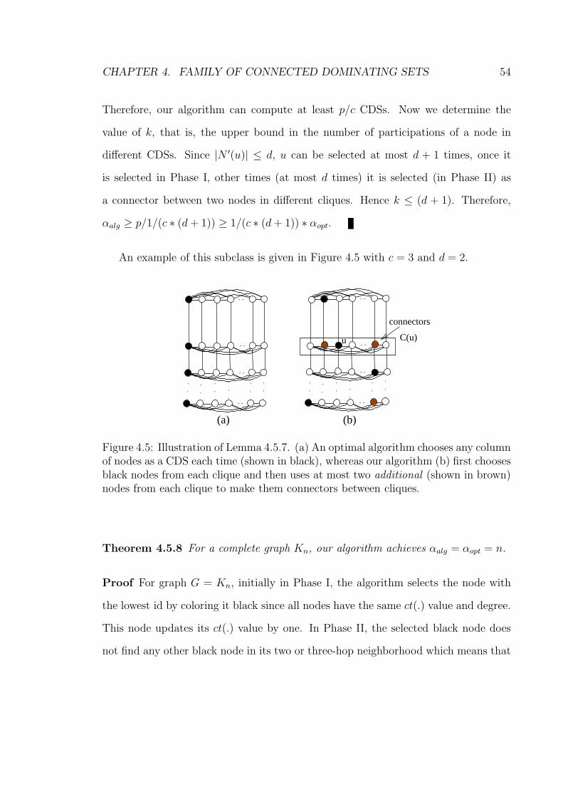
CHAPTER 4. FAMILY OF CONNECTED DOMINATING SETS 54
Therefore, our algorithm can compute at least p/c CDSs. Now we determine the
value of k, that is, the upper bound in the number of participations of a node in
different CDSs. Since |N ′(u)| ≤ d, u can be selected at most d + 1 times, once it
is selected in Phase I, other times (at most d times) it is selected (in Phase II) as
a connector between two nodes in different cliques. Hence k ≤ (d + 1). Therefore,
αalg ≥ p/1/(c ∗ (d + 1)) ≥ 1/(c ∗ (d + 1)) ∗ αopt.
An example of this subclass is given in Figure 4.5 with c = 3 and d = 2.
(b)(a)
u C(u)
connectors
Figure 4.5: Illustration of Lemma 4.5.7. (a) An optimal algorithm chooses any columnof nodes as a CDS each time (shown in black), whereas our algorithm (b) first choosesblack nodes from each clique and then uses at most two additional (shown in brown)nodes from each clique to make them connectors between cliques.
Theorem 4.5.8 For a complete graph Kn, our algorithm achieves αalg = αopt = n.
Proof For graph G = Kn, initially in Phase I, the algorithm selects the node with
the lowest id by coloring it black since all nodes have the same ct(.) value and degree.
This node updates its ct(.) value by one. In Phase II, the selected black node does
not find any other black node in its two or three-hop neighborhood which means that

CHAPTER 4. FAMILY OF CONNECTED DOMINATING SETS 55
no connector node is required. Thus we have exactly one node as CDS, i.e., |S1| = 1.
In the next round, the second lowest id node is selected and used as the only node in
the CDS (|S2| = 1), and so on. Thus we have a family S1, S2, · · · , Sm of CDSs, where
each set Si consists exactly of one node of Kn, all nodes in Kn are used in CDSs and
Si 6= Sj, i, j ∈ [1, m]. This means m = n and k = 1. Therefore, αalg = αopt = n.
4.5.3 Generating Disjoint CDSs: A counterexample
It seems reasonable that generating all possible disjoint CDSs for the problem of
maximizing α can obtain the maximum value of α. This is because the maximum
number of frequencies of a node in these sets will be guaranteed to be at most 1 and
maximizing the number of disjoint CDSs will maximize the value of α. However, in
this section we provide a counterexample showing that finding all possible disjoint
CDSs does not necessarily maximize α. Consider the geometric graph shown in Figure
4.6 (a). In this case, the number of possible disjoint CDSs is 1 (shown in Figure 4.6
(b)) for which the value of α is, α = m/k = 1. On the other hand, the value of α
can be maximized by finding overlapping CDSs as shown in Figure 4.6 (c)), where we
have 3 CDSs and the maximum number of participations of a node is 2 resulting in
α = 3/2 = 1.5.
4.6 Conclusion
In this chapter, we have presented a local algorithm for generating a family of CDSs
in sensor networks with a view to increasing the lifetime of nodes in the network. It
is shown that using the same CDS (even an optimal one) in sensor networks is not

CHAPTER 4. FAMILY OF CONNECTED DOMINATING SETS 56
(a)
(b)
(c)
Figure 4.6: A counterexample showing that obtaining the maximum number of dis-joint CDSs does not always maximize α.
a viable option since the nodes in the set quickly deplete their energy due to their
participation in every broadcast. Inspired by this observation, we develop a local
algorithm which takes care of this situation by generating other CDSs so that the
burden of broadcasting can be distributed over the nodes. We show an interesting
relationship between minimum vertex-cuts and CDSs, where the cardinality of a min-
imum vertex-cut limits the number of disjoint CDSs. We believe this is the first local
algorithm of its kind in the context of WSNs since previous algorithms mainly focus
on generating a single CDS of small size. Our algorithm obtains a constant factor
approximation of the value of α for a small subclass of UDGs. However it remains as
an interesting open problem to devise an algorithm (centralized or distributed) with
a constant approximation factor for UDGs.

Chapter 5
Domatic Partition
Here we consider a variant of the problem studied in the previous chapter, in which we
would like to generate as many disjoint dominating sets as possible, in other words,
we wish to maximize the number of dominating sets where the maximum number of
participations of a node in these sets is at most 1.
It is well known in WSNs research that distributing sensing and data gathering
tasks to a dominating set (preferably small-sized) helps prolong the network lifetime
by engaging such a subset of nodes for these tasks and letting other nodes go into the
energy-efficient sleep mode. For these types of applications, it is generally assumed
that the nodes in a dominating set need not form a connected subgraph since these
nodes are expected to individually sense the environment, collect and process the data
obtained and finally send them directly to the base station. Because they are busy
all the time for sensing, processsing, and transmitting data, nodes in the dominating
set quickly run out of energy. One possible way to overcome this situation is to
find a number of different dominating sets in the network and use them one by one
iteratively.
57

CHAPTER 5. DOMATIC PARTITION 58
In this chapter, we investigate the problem of finding the maximum number of
disjoint dominating sets called the domatic partition problem in UDGs. Although the
problem is NP-hard in general graphs [26], it is unknown whether the same is true for
UDGs. However, we present an algorithm towards solving this problem together with
experimental results and give a conjecture based on our results about the maximum
number of disjoint dominating sets in UDGs.
5.1 Introduction
Recall that a subset D ⊆ V of G = (V, E) is a dominating set if every vertex v ∈ V \D
has at least a neighbor in D. Here, we consider the problem of generating subsets
D1, D2, · · · , Dk such that each Di ⊆ V is a dominating set and Di ∩ Dj = φ, i 6= j,
and the objective is to maximize k. Dominating sets play an important role in saving
energy in individual sensors in WSNs which will be clear from the following discussion.
In general it is expected that the size of a dominating set be as small as possible.
Once deployed with a finite amount of energy, nodes in sensor networks continue
to spend energy sensing, gathering, and distributing data from the environment.
Since the nodes cannot be replenished with energy, one viable option is to prolong
the lifetime of the network by carefully utilizing the energy of individual nodes for
these tasks. In order to achieve this goal, one obvious way is to exploit the physical
proximity of nodes. Since closely positioned sensors in the plane sense almost similar
data, it is important to make active as few sensors as possible from such nearby
nodes, and put the rest of the nodes in the sleep mode to conserve energy. Thus, by
keeping only a few nodes active for gathering, processing, and transmitting data we
save valuable energy for other nodes. This naturally leads us to utilize the concept

CHAPTER 5. DOMATIC PARTITION 59
of a dominating set, where the nodes selected for carrying on the sensing tasks on
behalf of their nearby sensors form the dominating set. The smaller the size of the
dominating set the better is the energy saving since more sensors can be put in the
energy-efficient sleep mode.
However, as mentioned in the previous chapter, this kind of solution has one
major drawback in terms of balanced energy distribution among the sensors. This
is because the sensors in the dominating set will quickly consume their energy by
sensing and transmitting data while the other inactive sensors (that do not belong to
the dominating set and are in the sleep mode) can save their energy. This will result
in disproportionate energy consumption among the sensors which is not expected in
many applications where network lifetime depends on the functioning of individual
sensors. Even finding the minimum dominating set, that is, the one with the fewest
number of nodes, will be of no help in this scenario.
This problem can be alleviated if we replace an existing dominating set Di with
another disjoint dominating set Dj in the network and place the nodes in Di in the
sleep mode. This facilitates maximizing the network lifetime since the active role is
now shifted to a completely new set of nodes. Thus the basic idea is to find as many
disjoint dominating sets as possible and use each one for a certain amount of time
and then replace it with another one and so on. If initially all the nodes start with
the same amount of energy, then one can expect that the energy consumption will
likely be balanced among the nodes. The maximum number of disjoint dominating
sets is bounded by the minimum degree of the graph plus one, since a node can either
be in one of the dominating sets or be dominated by at least one of its neighbors. A
graph which possesses the maximum number of disjoint dominating sets given by the

CHAPTER 5. DOMATIC PARTITION 60
bound is called domatically full. An example of a domatically full graph is given in
Figure 5.1(a). However, not all graphs are domatically full (see Figure 5.1(b)).
1
2 3
42
4 1
3
1
2
1
2
(b)(a)
Figure 5.1: (a) In this 3-connected graph (it is a general graph, not a UDG), wehave four disjoint dominating sets. Each dominating set is denoted by the same digit.Hence the domatic partition of this graph is 4. (b) The graph does not admit morethan two disjoint dominating sets although the minimum degree plus one is 3.
If we can have a family D1, D2, · · · , Dk of disjoint dominating sets in G = (V, E),
where Di ⊆ V , then we can employ the first dominating set D1 for a certain time
interval, say, [0, t1]. Thereafter, we can replace D1 by D2 and make D2 active for
the [t1, 2 ∗ t1] time period, and so on until we are finished with Dk being active
for [(k − 1) ∗ t1, k ∗ t1] time interval in which case we can repeat the whole process
starting from D1. It is clear that the larger the value of k, the longer we can prolong
the lifetime of the network. However, as mentioned above, the optimal (maximum)
value of k can be at most δ + 1, where δ is the minimum degree in G. Here, we
investigate the problem of finding the maximum number of disjoint dominating sets
(called the domatic partition problem), that is, the maximum value of k (called the
domatic partition number) in the special case of UDGs.

CHAPTER 5. DOMATIC PARTITION 61
5.2 Related Work
The minimum dominating set problem is one of the classical graph theory problems
that has been extensively studied [26, 41] and proven to be NP-hard in general.
For general graphs, one can show [20] that unless NP ⊆ DTIME (nO(log log n)), no
polynomial time algorithm can approximate the minimum dominating set problem
better than ln4− o(ln4), where 4 is the maximum degree of the graph. In UDGs,
the minimum dominating set problem still remains NP-hard [16]. However, it can be
approximated within a constant factor. In [1], Alzoubi et al. show that the size of any
MIS in a UDG is at most 4 times the size of the optimal dominating set. Since an MIS
is also a dominating set, this proves that a dominating set is at most 4 times the size
of the optimal dominating set. The dominating set problem has also been studied in
distributed settings. In a distributed environment, a constant factor approximation
ratio is obtained in [42] in O(log2 n) time. Luby [55] gives a randomized distributed
algorithm to find a constant approximation to the minimum dominating set problem
in O(log n) time.
However, all the aforementioned algorithms focus on finding a single ‘small’ sized
dominating set in the graph. As pointed out earlier, the domatic partition problem
is one of the problems proved to be NP-hard in [26] for general graphs. This problem
has been throughly studied by Feige et. al. [21] who provide some useful insights
about the problem for general graphs. In [21], the authors prove that every graph with
maximum degree 4 and minimum degree δ contains a domatic partition of size (1−
o(1))(δ + 1)/ ln4. They show that 1/(ln4) is the best possible approximation ratio
for this problem for general graphs unless NP ⊆ DTIME (nO(log log n)). A natural
greedy approach to this problem is to find as many small-sized disjoint dominating

CHAPTER 5. DOMATIC PARTITION 62
sets as possible. However, Fujita [22] studies several variants of such greedy algorithms
and shows that their performance ratio is no better than 1/√
n.
In [58], the authors look at a variant of the domatic partition problem and propose
randomized approximation algorithms for maximizing the network lifetime. The prob-
lem considered in the paper is called the Maximum Cluster-Lifetime problem, where
they aim to find an optimal schedule consisting of a set of pairs (D1, t1), · · · , (Dk, tk),
where Di is a dominating set and ti is the time during which Di is active. That
is, D1 is active in the time-interval (slot) [0, t1] and Di is active in the time-interval
[∑i−1
j=0 tj,∑i
j=0 tj]. The lifetime of a schedule is defined as L(S) =∑k
i=1 ti. The prob-
lem then asks for the schedule S with maximum length L(S) such that∑
i:v∈Diti ≤ bv,
where bv is the maximum time node v can be in a dominating set. The randomized
algorithms compute a schedule which is an O(log n) approximation to the Maximum
Cluster-Lifetime problem with probability at least 1 − o(1/n).
The authors in [69] propose a centralized algorithm, without providing any worst
case analysis or bound, to generate a number of disjoint dominating sets in order to
cover a geometrical region by a network of nodes for as long as possible. A general
version of the domatic partition called the k-domatic partition (k ≥ 2), where in each
dominating set a node is dominated by at least k nodes, is considered in [62]. The
authors propose three deterministic distributed algorithms. Each of the algorithms
constructs a k− domatic partition of size at least a constant fraction of the largest
possible (k − 1)-domatic partition.
The reminder of this chapter is organized as follows. In Section 5.3 we provide
definitions and assumptions that are used throughout the chapter. The proposed

CHAPTER 5. DOMATIC PARTITION 63
algorithm is presented in Section 5.4. We provide a theoretical analysis of our algo-
rithm in Section 5.5 followed by experimental results in Section 5.6. We conclude in
Section 5.7.
5.3 Preliminaries and Definitions
Our algorithm to find disjoint dominating sets operates in time-slots (we use time-slots
as iterations interchangeably) where at each time-slot i we construct a dominating
set Di (where Di ∩ Dj = φ, i 6= j and i, j ≥ 1). We color the nodes in Di with color
class i. By δ = minv∈V deg(v), we mean the minimum degree in the graph.
5.3.1 Compatible and Incompatible nodes
A node v ∈ N [u] is called an uncovered neighbor of u at iteration i if there is no
node w ∈ Di that is a neighbor of v (we say that v is not covered by any node in
Di). The total number of uncovered neighbors of u (including u) in iteration i is
denoted as, uncovi(u) = |v|v ∈ N [u], vw /∈ E, w ∈ Di ∧ v 6= w|. The dom number
of node u, denoted by dom(u), is the number of neighbors (including u) that belong
to some dominating sets, that is, dom(u) = |v|v ∈ N [u], v ∈ Dj, j ≥ 1|. Each
node u maintains a triple at iteration i, ti(u) =≺ 1/uncovi(u), dom(u), id which is
updated in each iteration. If uncovi(u) = 0, then we assign uncovi(u) = 1/(n + 1),
where n = |V |. We call a node u compatible if uncovi(u) 6= 1/(n + 1), otherwise
it is incompatible. For any two compatible nodes u, v, we say u is smaller than v
in iteration i if ti(u) is lexicographically smaller than ti(v) and denote the order by
ti(u) < ti(v). Note that comparison is done only between compatible nodes.

CHAPTER 5. DOMATIC PARTITION 64
5.4 Algorithm for the Domatic Partition Problem
In this section we informally describe our algorithm. The algorithm works in iterations
starting from iteration 1 and in each iteration i (i ≥ 1), we compute a dominating
set Di such that Di ∩ Dj = φ, i 6= j, i, j ≥ 1. The algorithm runs for at most
δ + 1 iterations. Specifically, it stops in iteration j if we cannot form a new disjoint
dominating set Dj or we have j = δ+1. If j = δ+1 then we have reached the optimal
(maximum) number of disjoint dominating sets. Otherwise, j − 1 is the maximum
number of disjoint dominating sets D1, D2, · · · , Dj−1 returned by the algorithm. This
algorithm has appeared in [38].
Begin with iteration 1. Let D′1 = φ be a null set that expands gradually as
nodes are inserted into it during the execution of the algorithm. First, we compute
a triple for each node in G and select the smallest one among the compatible nodes.
From the triples it is easy to see that we always find such a single node. Let u
be the smallest node. We color u 1, add u to D′1 (note that D′
1 is a temporary
set that grows as dominating nodes are added to it). We update t1(v), v ∈ N [u].
Then we pick the smallest compatible node in V \ D′1, color it 1, insert into D′
1 and
update the nodes’ triples. At each selection of a node u in D′1, we make at least
one node incompatible. We repeat the process until all nodes become incompatible.
Assign D1 = D′1. We claim that nodes in D1 form a dominating set. At this stage,
∀u∈V uncovi(u) = 1/(n + 1) and ∀v∈V \D1dom(v) ≥ 1.
We now describe in general how a dominating set Di is formed at iteration i ≥ 2.
First, initialize ∀u∈V uncovi(u) = deg(u) + 1 and let D′i = φ. (As before D′
i is a
temporary set used in the i-th iteration to contain the dominating nodes that are
added to it as the algorithm progresses and when D′i becomes a dominating set we
CHAPTER 5. DOMATIC PARTITION 65
rename it as Di). Select the smallest node among the compatible nodes in V \ (D1 ∪
D2 · · ·Di−1∪D′i), color it i, and add it to D′
i. Update the triples of the corresponding
nodes. Then find the smallest compatible node in V \ (D1 ∪ D2 · · ·Di−1 ∪ D′i), color
it i and insert it into D′i. Update the triples of the nodes whose uncovi(.), dom(.)
values are changed. Continue this process until one of following cases occurs
Case I: all nodes become incompatible
or
Case II: V \ (D1 ∪D2 · · ·Di−1 ∪D′i) = φ and there exists at least one compatible
node in G
or
Case III: V \ (D1 ∪ D2 · · ·Di−1 ∪ D′i) 6= φ and there exists a node u such that
∀u′ ∈ N [u], u′ ∈ D1 ∪ D2 · · ·Di−1 ∪ D′i.
If Case (I) is satisfied then assign Di = D′i and we have already constructed the
i-th dominating set Di and next iteration i + 1 is invoked to generate Di+1.
On the other hand, if V \ (D1 ∪ D2 · · ·Di−1 ∪ D′i) = φ and there is at least a
compatible node (Case (II)), then we cannot form the current dominating set and
the algorithm reports that i − 1 is the maximum number of disjoint dominating sets
and the execution ceases. This is because there is no node to be included in D′i and
some nodes are still uncovered. Similarly if Case (III) is satisfied then the algorithm
terminates and reports i − 1 as the maximum number of disjoint dominating sets.
This is because there is no neighborhood N [u] of u from which we can select a node
to cover u.
Let j represent the maximum number of dominating sets returned by our algo-
rithm, that is, the algorithm constructs D1, D2, · · · , Dj disjoint dominating sets.

CHAPTER 5. DOMATIC PARTITION 66
Algorithm for the Domatic Partition ProblemInput: A UDG G = (V, E)Output: j disjoint dominating sets D1, D2, · · · , Dj
1: Compute t1(u) =≺ 1/uncov1(u), dom(u), id , ∀u ∈ V2: D′
1 = φ;i = 13: while i ≤ (δ + 1)4: Find the smallest compatible5: node u in V \ (D′
1 ∪ D′2 ∪ · · · ∪ D′
i)6: if there is such u then7: D′
i = D′i ∪ u
8: else9: if Case (II) or Case (III) is satisfied then10: j = i − 111: break12: else13: if all nodes are incompatible then14: Di = D′
i
15: i = i + 116: j = i17: D′
i+1 = φ18: endif19: endif20: endif21: update ∀u ∈ V ti(u) =≺ 1/uncovi(u), dom(u), id 22: endwhile
Figure 5.2: An algorithm for the domatic partition problem.
5.4.1 Algorithm Illustration
We illustrate the execution of our algorithm through an example shown in Fig-
ure 5.4. Nodes are marked in lower-case letters below the nodes and integers s
on the left of nodes denote the dominating sets Ds to which the nodes belong.
In the first iteration, we find node a is the smallest compatible node (t1(a) =≺
1/uncov1(a), dom(a), id(a) =≺ 1/8, 0, id(a) ) in the graph, where uncov1(.) =
deg(.). Select a, add to D′1 and we update triples t1(.)’s of nodes whose uncov1(.) and
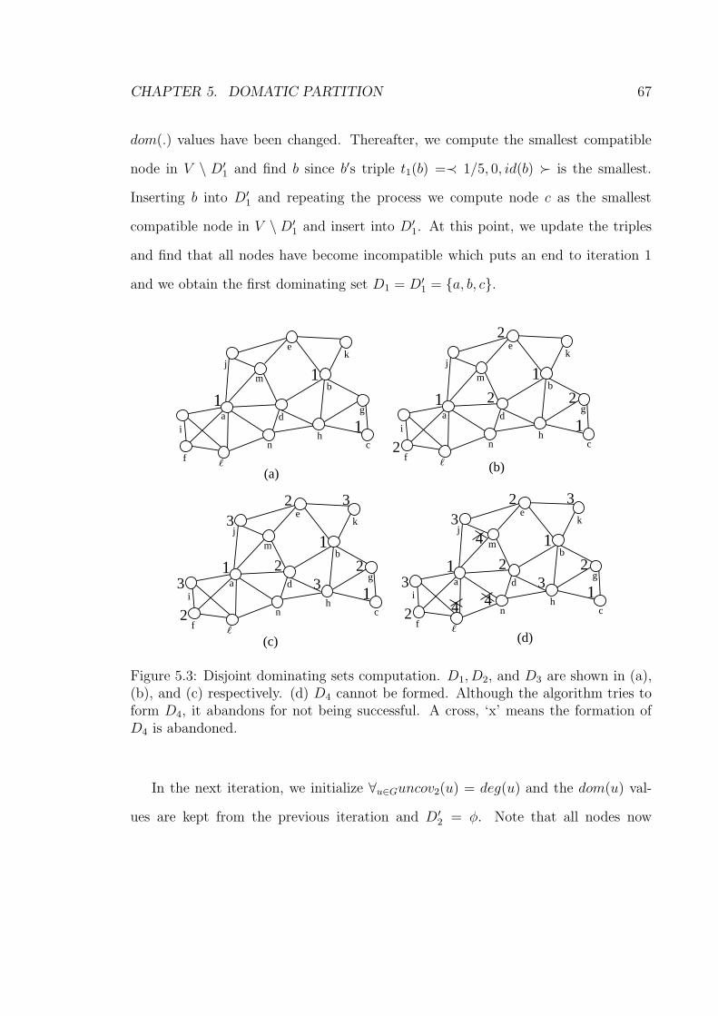
CHAPTER 5. DOMATIC PARTITION 67
dom(.) values have been changed. Thereafter, we compute the smallest compatible
node in V \ D′1 and find b since b′s triple t1(b) =≺ 1/5, 0, id(b) is the smallest.
Inserting b into D′1 and repeating the process we compute node c as the smallest
compatible node in V \ D′1 and insert into D′
1. At this point, we update the triples
and find that all nodes have become incompatible which puts an end to iteration 1
and we obtain the first dominating set D1 = D′1 = a, b, c.
a
2
2
1b
1
2d
e
f
g
1c
hi
k
m
j
2
n
(b)
(d)
a
2
2 3
1b
1
2d 3
e
f
g
1c
3h
i
k
m
3j
2
4 4n
4
a1
b1
d
e
f
g
1c
hi
k
m
j
n
a
2
2 3
1b
1
2d 3
e
f
g
1c
3h
i
k
m
3j
2
n
(a)
(c)
`
`
`
`
Figure 5.3: Disjoint dominating sets computation. D1, D2, and D3 are shown in (a),(b), and (c) respectively. (d) D4 cannot be formed. Although the algorithm tries toform D4, it abandons for not being successful. A cross, ‘x’ means the formation ofD4 is abandoned.
In the next iteration, we initialize ∀u∈Guncov2(u) = deg(u) and the dom(u) val-
ues are kept from the previous iteration and D′2 = φ. Note that all nodes now
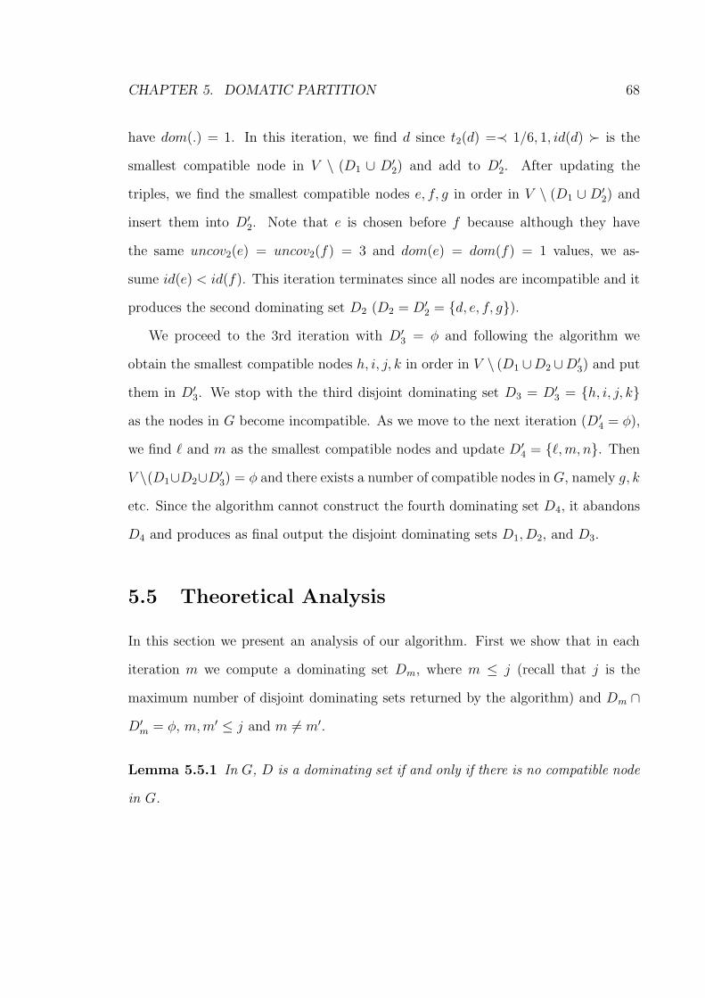
CHAPTER 5. DOMATIC PARTITION 68
have dom(.) = 1. In this iteration, we find d since t2(d) =≺ 1/6, 1, id(d) is the
smallest compatible node in V \ (D1 ∪ D′2) and add to D′
2. After updating the
triples, we find the smallest compatible nodes e, f, g in order in V \ (D1 ∪ D′2) and
insert them into D′2. Note that e is chosen before f because although they have
the same uncov2(e) = uncov2(f) = 3 and dom(e) = dom(f) = 1 values, we as-
sume id(e) < id(f). This iteration terminates since all nodes are incompatible and it
produces the second dominating set D2 (D2 = D′2 = d, e, f, g).
We proceed to the 3rd iteration with D′3 = φ and following the algorithm we
obtain the smallest compatible nodes h, i, j, k in order in V \ (D1 ∪D2 ∪D′3) and put
them in D′3. We stop with the third disjoint dominating set D3 = D′
3 = h, i, j, k
as the nodes in G become incompatible. As we move to the next iteration (D′4 = φ),
we find ` and m as the smallest compatible nodes and update D′4 = `, m, n. Then
V \(D1∪D2∪D′3) = φ and there exists a number of compatible nodes in G, namely g, k
etc. Since the algorithm cannot construct the fourth dominating set D4, it abandons
D4 and produces as final output the disjoint dominating sets D1, D2, and D3.
5.5 Theoretical Analysis
In this section we present an analysis of our algorithm. First we show that in each
iteration m we compute a dominating set Dm, where m ≤ j (recall that j is the
maximum number of disjoint dominating sets returned by the algorithm) and Dm ∩
D′m = φ, m, m′ ≤ j and m 6= m′.
Lemma 5.5.1 In G, D is a dominating set if and only if there is no compatible node
in G.

CHAPTER 5. DOMATIC PARTITION 69
Proof We prove the lemma by contradiction. Assume that D is a dominating set
and there exists at least one compatible node v in G. This means either v or some of
its neighbors are not covered by any node w ∈ D. Then there can be two situations,
either (i) only v is uncovered or (ii) more than one node in N [v] is uncovered. In any
case D is not a dominating set in G, a contradiction.
Now we prove the other direction. Again, assume for contradiction that all nodes
are incompatible and D is not a dominating set in G. By definition, if all nodes are
incompatible then each of them is dominated by some nodes in D, contradicting the
fact that D is not a dominating set in G.
In the following, we prove that our algorithm guarantees that it can always gen-
erate the first dominating set in UDGs.
Lemma 5.5.2 For D1 only Case (I) is satisfied (Case (II) and Case (III) are never
reached by the algorithm while computing D1). Hence j ≥ 1 (the number of dominat-
ing sets returned by the algorithm).
Proof Assume for contradiction that Case (II) is reached while D′1 (recall that D′
1
is a temporary set which is assigned to D1 when D′1 becomes a dominating set in G)
is being computed. Since Case (II) is satisfied, V \ D′1 = φ and we have at least one
compatible node. But this is a contradiction since if V \ D′1 = φ, D′
1 is already a
dominating set, and there cannot be any compatible nodes in G.
Similarly assume Case (III) is satisfied while computing D′1. Then V \D′
1 6= φ and
there is a node u such that ∀u′ ∈ N [u], u′ ∈ D′1. This is a contradiction because this
shows that u as well as all its neighbors belong to D′1 and hence D′
1 is a dominating
set.
CHAPTER 5. DOMATIC PARTITION 70
It is easy to see that Case (I) must be satisfied if Case (II) or Case (III) is not
encountered. Thus the smallest value of j can be at least one and hence for Line 10
j ≥ 1.
As our objective is to generate disjoint dominating sets, in the following we show
that the algorithm can indeed produce dominating sets in G such that any pair
of dominating sets are mutually disjoint, i.e., there are no two dominating sets in
D1, D2, · · · , Dj which have a common node.
Lemma 5.5.3 Each Dp is a dominating set and Dp ∩ Dq = φ for 1 ≤ p < q ≤ j.
Proof First we prove that Dp is a dominating set by contradiction. Suppose Dp
is not a dominating set at the end of iteration p. Then there is some node v not
dominated by any nodes in Dp. That is, uncovp(v) ≥ 1 which implies that v is a
compatible node. This is a contradiction (from Lemma 5.5.1).
Now we show that Dp ∩ Dq = φ for 1 ≤ p, q ≤ j and p 6= q. Without loss of
generality, assume q > p and Dp∩Dq 6= φ. Therefore there exists at least one node in
Dp∩Dq. Let u ∈ Dp∩Dq. Assume M = V \(D1∪D2 · · ·∪Dp), where dominating sets
D1, D2, · · · , Dp have already been computed. In computing Dq in the q-th iteration,
we select nodes from M . Thus if u is picked in Dq then either u does not belong to
Dp or Dp is an empty set, yielding a contradiction.
In the following we present the time complexity of our algorithm.
Lemma 5.5.4 The time complexity of the algorithm is O(n3).
Proof The while loop in the algorithm runs for δ + 1 times which could be as large
as O(n). For each iteration of the loop, to find the smallest compatible node it takes

CHAPTER 5. DOMATIC PARTITION 71
O(n) time. Also in each iteration of the loop, for each node that is inserted in the
current dominating set we update the triples of all its neighbors and doing so takes
O(n2). Thus the time complexity of the algorithm is O(n3).
5.6 Simulations
We conducted extensive simulations on random networks to study the performance of
the proposed algorithm. In this section, we provide and analyze experimental results
regarding domatic partitions produced by our algorithm and compare them with the
optimal (maximum) domatic partition. In the experiment, first we obtain UDGs G by
generating a set nodes uniformly and randomly in the plane and test the connectivity
of G and compute the minimum degree of G. If the underlying graphs are connected
then we apply the algorithm to construct disjoint dominating sets and analyze its
performance in these random graphs.
5.6.1 Experimental Setup
Experiments are done using our own simulator in Java. In order to evaluate the av-
erage performance critically, we choose square fields of different sizes namely, 600m
x 600m, 500m x 500m, 400m x 400m, and 300m x 300m. For each of these squares,
n ∈ 100, 200, 300, · · · , 900, 1000 nodes are generated randomly from a uniform dis-
tribution. The transmission range of all nodes is set to 80m. For each of the squares
and for each value of n we generate 100 different netwrok topologies, and run the al-
gorithm which produces a number of disjoint dominating sets. The choice of different
field sizes for the same input size helps generate relatively sparse (for larger squares)

CHAPTER 5. DOMATIC PARTITION 72
and dense graphs (for smaller squares) to evaluate the algorithm in both situations.
5.6.2 Experimental Results
Setting the transmission range to 80m for all nodes, we apply our algorithm in a 600m
x 600m square with n = 100 and compute the domatic partition (DP) number (i.e.,
the number of disjoint dominating sets) and compare with the optimal DP number.
Then we generate 100 random graphs successively and for each graph we compute
and compare these DP numbers (one by the algorithm and the other is the optimal
value). In order to compute the optimal DP value we use an upperbound on the
optimal value, which is the minimum degree of G plus 1. Finally, we obtain the
average DP number by our algorithm and compare it with the average optimal DP
number of all the 100 random topologies. Then the value of n is incremented by 100
(i.e., n = 200) and the whole procedure is repeated. We continue incrementing the
value of n by 100 each time and repeating the experiment until n = 1000.
To obtain more convincing results and to see how the results vary in terms of the
DP number, we apply the algorithm and perform the same procedure in squares of
sizes 500m x 500m, 400m x 400m, and 300m x 300m, varying n from 100 to 1000
as before and generating 100 different topologies for each value of n. Changing the
sizes of squares affects the degrees of nodes, that is, the smaller the area of the field
the denser the graphs are and hence the larger the minimum degrees of the graphs.
Intuitively the experiment show that for smaller field sizes the DP numbers are greater
than that of larger fields for the same values of n.
The results are plotted in Figure 5.4, where the x-axis shows the number of nodes
in the generated topology and the y-axis represents the average DP number returned

CHAPTER 5. DOMATIC PARTITION 73
100 200 300 400 500 600 700 800 900 10000369
1215182124273033363942454851545760
Number of nodes
Dom
atic
par
titio
n (D
P)
and
Opt
imal
DP
300x300 Alg300x300 Opt400x400 Alg400x400 Opt500x500 Alg500x500 Opt600x600 Alg600x600 Opt
Figure 5.4: Showing the comparison between the average domatic partition (DP)number returned by the algorithm and the average optimal DP number (minimumdegree of G plus 1) in different field sizes for each value of n ∈ 100, 200, · · · , 1000.
by the algorithm (shown as non-solid lines, marked as ‘Alg’ at the top-left corner of
the figure) and the average optimal (maximum) DP number (shown as solid lines,
marked as ‘Opt’ at the top-left corner of the figure). As can be understood from the
figure, the bottom line pair (solid and non-solid line) shows the average results of the
algorithm and the optimal DP numbers when the input field size is 600m x 600m.
For smaller values of n = 100-400, the average DP number almost coincides with the
optimal and the values are around 3-5. For higher values of n = 900-1000, the DP
number by the algorithm and optimal numbers are in between 9-12. Other pairs of
lines are similarly shown with their respective field sizes. In these average cases our
experimental results are close to the optimal for all values of n = 100-1000 and in
all different sizes of fields. It may be worth mentioning that for smaller values of
n <= 400, the maximum difference between our average DP value and the optimal

CHAPTER 5. DOMATIC PARTITION 74
is 2 (additive factor) and for larger values of n the maximum difference is 3 (additive
factor).
5.6.3 Cardinalities of Dominating Sets
We also provide some interesting results regarding the average number of nodes in
each of the dominating sets. For each run of the algorithm to compute the DP
number for a certain value of n, we keep track of the minimum and maximum sizes
of dominating sets among the disjoint dominating sets. Since 100 topologies are
generated for each value of n, we compute the averages of the minimum and maximum
sizes of dominating sets.
100 200 300 400 500 600 700 800 900 1000579
11131517192123252729313335373940
Number of nodes
Avg
. Min
imum
siz
e of
dom
inat
ing
sets
300x300400x400500x500600x600
Figure 5.5: Showing the average minimum cardinality of dominating sets found byour algorithm for different values of n.
In Figures 5.5 and 5.6 we plot these values where in the x−axis the number of
nodes and in the y-axis the average sizes (the average minimum size in Figure 5.5

CHAPTER 5. DOMATIC PARTITION 75
100 200 300 400 500 600 700 800 900 100010
12
14
16
18
20
22
24
26
28
30
32
34
36
38
40
42
4445
Number of nodes
Avg
. Max
imum
siz
e of
dom
inat
ing
sets
300x300400x400500x500600x600
Figure 5.6: Showing the average maximum cardinality of dominating sets found byour algorithm for different values of n.
and the average maximum size in 5.6) of dominating sets are shown. In general, the
results show that, for UDGs, the denser the graphs are the smaller the cardinalities
of dominating sets. In an intuitive sense, this happens since in a denser graph each
node has relatively many neighbors and when it becomes a dominating node it can
dominate many nodes. For example, in Figure 5.5, for a 300m x 300m field, the
average minimum size of dominating sets varies from 8 − 10 for all values of n used
in our experiments whereas for a 600m x 600m square the average minimum size
fluctuates from 16 to 35. Similar results are shown in Figure 5.6 for the average
maximum size of dominating sets. A sample output of the algorithm is shown in
Figure 5.7.
The mean or average of a value does not reflect the amount of variation among
the values. In order to get an idea how the DP numbers spread out over different

CHAPTER 5. DOMATIC PARTITION 76
Figure 5.7: A sample output with 200 nodes distributed on 400m x 400m square fieldwhere both the optimal DP and the computed DP numbers are 6 (shown in 6 differentcolors).
values, we compute the standard deviation of the DP numbers (shown in Figure 5.8).
The smaller the standard deviation the closer the DP numbers to the average value.
As shown in the figure, although the standard deviations for different values of n
are smaller (less than 1) and do not vary a lot, they differ in different field sizes.
For larger field size (e.g., 600x600) the nodes are generally more sparsely distributed
and hence the minimum degree of the underlying graph is relatively small. In such
situations, the fluctuations in the values of DP numbers are small for such randomly
drawn graphs. Similar reasoning can be applied to smaller field sizes. However, as
shown the standard deviations seem to be consistent and reasonably small for all
different field sizes.

CHAPTER 5. DOMATIC PARTITION 77
100 200 300 400 500 600 700 800 900 1000
0.4
0.5
0.6
0.7
0.8
0.9
1
Number of nodes
Sta
ndar
d D
evia
tion
500x500
600x600
400x400
300x300
Figure 5.8: Showing standard deviations of DP numbers for different size of fields.
5.6.4 Conjecture about the Maximum Number of Disjoint
Dominating Sets
UDGs have a nice property that for any node in the graph, there can be at most
five independent nodes in its neighborhood. In other words, for a node u we need
at most 5 nodes to cover (dominate) all its neighbors. This result can be further
strengthened. In a constant-size neighborhood (e.g., a k-hop neighborhood) UDGs
at most a constant number of independent nodes. This is a strong property of UDGs
and other growth-bounded graphs (which also have the same property). Utilizing this
property and depending on the experimental results, we have the following conjecture:
Conjecture 5.6.1 For UDGs, the domatic partition problem can be solved within a
constant factor of the optimal.

CHAPTER 5. DOMATIC PARTITION 78
5.7 Conclusion
In this chapter, we have presented an algorithm based on domatic partition for max-
imizing the lifetime of WSNs. We have provided extensive simulation results to
assess the performance of the algorithm where the experiments show ‘good’ results.
However, one intriguing open question is to come up with an algorithm that gives
an approximation factor (preferably ‘small’) for UDGs. We believe that a constant
factor algorithm is achievable by utilizing the structural properties of UDGs. For
example, a node can have at most five independent nodes in its neighborhood. For
UDGs, the only known factor for this domatic partition problem is logarithmic and
obtained by a randomized algorithm [58]. Since centralized algorithms do not gener-
ally scale up for large networks, distributed algorithms are sought for large wireless
sensor networks. Thus it would be challenging to find a distributed solution with a
small constant approximation factor for the domatic partition problem in UDGs.

Chapter 6
Target Monitoring
In this chapter, we consider the following target monitoring problem: Given a set of
stationary targets T = t1, · · · , tm and a set V = v1, · · · , vn of sensors, the target
monitoring problem asks for generating a family of subsets of sensors V1, · · · , Vs called
the monitoring sets, such that each Vi monitors all targets. In doing so, the objective
of this problem is to maximize z = s/k, where k=maxvj∈V |i : vj ∈ Vi|. Maximizing
z means generating a large number of monitoring sets and minimizing the number of
frequencies of a sensor in these sets.
As energy is one of the main issues of WSNs and sensing consumes energy, max-
imizing z may have a direct impact in prolonging the lifetime of such networks.
Basically, the problem is related to the one we studied in Chapter 4. Unlike finding
a family of CDSs, here we generate a family of subsets of nodes (nodes in a subset
are not necessarily connected) each of which monitors all the targets (the number of
targets is independent of the underlying UDG). However, by maximizing z, we dis-
tribute the monitoring responsibilities to all sensors as equally as possible and at the
same time, reduce the participations of individual sensors in these monitoring sets.
79

CHAPTER 6. TARGET MONITORING 80
Towards achieving this goal, a local algorithm is presented. The algorithm is
simple and requires each node to know only its 2-hop neighborhood. Furthermore,
nodes do not need to know their geographic positions. In short, the main idea is that
each node maintains a record (counter, id), where counter is the number of previous
monitoring sets in which the node has been selected to monitor the targets. To select
sensors for the next monitoring set, for each target, the lexicographically smallest
sensor covering it, is selected. We provide special instances where the algorithm
obtains an optimum result. As a by-product of the algorithm, it is shown that the
size of a monitoring set is at most a constant times the size of a minimum monitoring
set when the number of targets is a constant. We present extensive simulation results
to evaluate the performance of the algorithm in randomly generated UDGs.
6.1 Introduction
Consider Figure 6.1, where a network of six nodes is shown. Nodes u, w are within
their transmission range and can sense a target (shown as a rectangle) as it falls
in their sensing range. Node v can also sense the target but none of u or w is v’s
neighbor. When a node remains active and senses a target in its sensing range, we
say the node monitors the target (and the set of all such monitoring nodes forms a
monitoring set). After the ad hoc network is formed, nodes begin sensing the environ-
ment and depending on the application, such as target tracking, target monitoring,
area coverage, and so on, they cooperate by sending and receiving sensed information
among their close neighborhood.
However, the more a node engages in sensing targets (in their vicinity) and trans-
mitting, the more energy it consumes. As previously mentioned, in most applications
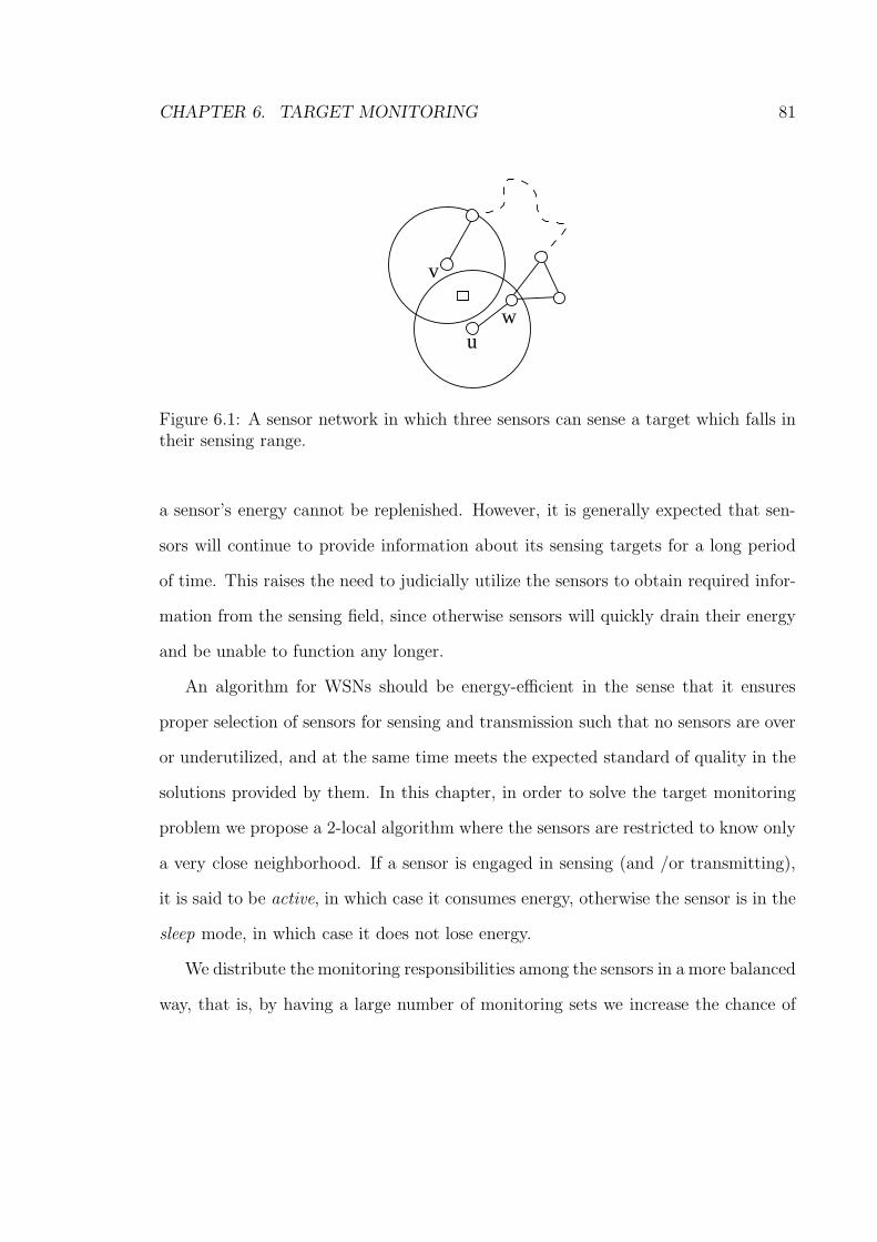
CHAPTER 6. TARGET MONITORING 81
uw
v
Figure 6.1: A sensor network in which three sensors can sense a target which falls intheir sensing range.
a sensor’s energy cannot be replenished. However, it is generally expected that sen-
sors will continue to provide information about its sensing targets for a long period
of time. This raises the need to judicially utilize the sensors to obtain required infor-
mation from the sensing field, since otherwise sensors will quickly drain their energy
and be unable to function any longer.
An algorithm for WSNs should be energy-efficient in the sense that it ensures
proper selection of sensors for sensing and transmission such that no sensors are over
or underutilized, and at the same time meets the expected standard of quality in the
solutions provided by them. In this chapter, in order to solve the target monitoring
problem we propose a 2-local algorithm where the sensors are restricted to know only
a very close neighborhood. If a sensor is engaged in sensing (and /or transmitting),
it is said to be active, in which case it consumes energy, otherwise the sensor is in the
sleep mode, in which case it does not lose energy.
We distribute the monitoring responsibilities among the sensors in a more balanced
way, that is, by having a large number of monitoring sets we increase the chance of

CHAPTER 6. TARGET MONITORING 82
selecting all sensors in the network in these sets, and by minimizing the number of
participations of individual nodes in these sets, we reduce the possibility of selecting
the same nodes. Therefore, as nodes in the network are put in the active and the
energy-efficient sleep mode alternatively, the lifetime of individual nodes is prolonged
and hence the lifetime of the network. Another important aspect of the algorithm is
the issue of scalability. Since it is a local algorithm where the nodes need to know
only their 2-hop neighborhood, it is a suitable candidate for the target monitoring
problem in large WSNs.
The rest of the chapter is organized as follows. In Section 6.2 some related work
about the problem is described. In Section 6.3 we provide definitions and assumptions
that are used throughout the chapter. The algorithm is presented in Section 6.4 and
a theoretical analysis of the algorithm follows in Section 6.5. Experimental results
are presented in Section 6.6 with conclusion in Section 6.7.
6.2 Related Work
Coverage (also called monitoring) has been one of the important topics in WSNs and
has received a lot of attention during the past several years [8, 10, 11, 24, 47, 31, 67,
71, 78]. The main goal of most of the work is to devise scheduling algorithms such
that individual sensors in the network are assigned time-slots which indicate to them
during which time-slots they will be active and during which rounds they will be in
the sleep mode. When a number of sensors monitor a certain area or a target, it is
generally possible to monitor the area or the target by a small subset of them. So, it
is redundant to make all the sensors active at the same time for the monitoring. This
observation leads researchers to devise efficient algorithms such that at any time only

CHAPTER 6. TARGET MONITORING 83
a small number of sensors are set as active to monitor the area or the targets.
In [8] the authors consider the target coverage problem with the goal to minimize
energy consumption. Given a set of targets, they propose an energy-efficient central-
ized scheme to provide coverage to all the targets by disjoint sets of sensors. They
divide the sensor set into disjoint subsets and activate each set to perform the cover-
ing task. Basically, their main idea is to generate as many disjoint sets of sensors as
possible such that each set covers all the targets (this is similar to the domatic par-
tition problem). However, the algorithm is centralized and does not scale for larger
networks.
In [69] the authors address the area coverage problem where their algorithm works
in two phases. In the first phase, the algorithm determines how many sensors cover
the different parts of the monitored area. Like the algorithm in [8], the second phase
allocates sensors into mutually independent sets where some set is active at any
time to provide the area coverage. The algorithm is also centralized and the authors
do not provide any theoretical results regarding the performance of their algorithm.
Simulation results show that the algorithm achieves significant power savings (by
generating more disjoint sets of sensors) in performing area coverage.
The work relevant to ours is [9], where the authors consider the target coverage
problem by a set of subsets of nodes while the subsets do not need to be disjoint.
They call this the maximum set cover (MSC) problem and present two centralized
algorithms, one based on linear programming and the other is a greedy algorithm.
They do not provide any theoretical analysis of their algorithms and give simulation
results to verify their approaches. Here, we consider the target monitoring problem
where we focus on generating a number of monitoring sets and at the same time

CHAPTER 6. TARGET MONITORING 84
reducing the number of participations of each node in these generated sets.
A recent result also related to our problem is described in [7], where the authors
consider the monitoring schedule problem: Given a set of sensors and a set of targets,
it is required to find a partition of the sensor set such that each part can monitor
all targets. Each part of the partition is used for one unit of time and the goal is to
maximize the number of parts in the partition. They present a randomized distributed
algorithm which generates at least (1−ε)∗opt (0 < ε < 1) parts, with high probability,
where opt is the maximum number of parts in the partition. However, they make the
assumption that the nodes must know their geographic positions.
The authors also suggest that by modifying their algorithm they can find a con-
stant approximation factor for the problem and the sensors do not need to know their
geographic positions. Our work is related to theirs in the sense that we maximize
the number of parts while trying to reduce the use of the same nodes in these parts.
Besides, ours is a deterministic algorithm as opposed to their randomized one and
the assumption that the sensors know their positions is excluded.
6.3 Preliminaries and Some Definitions
The target set is denoted as T = t1, · · · , tm, where ti is a target. The set of targets
monitored by node u is referred to as T (u). For u and t ∈ T (u), Tt(u) represents the
set of nodes in N2[u] that monitors the target t (i.e., Tt(u) = t|t ∈ T (u) ∩ T (v), v ∈
N2[u]).
Each node u maintains an ordered pair at each iteration i (initially i = 1),
pi(u) =≺ (cti(u), id(u)) , where the first element cti(u) (also called the counter)
denotes the number of monitoring sets in which u has already participated. Initially,

CHAPTER 6. TARGET MONITORING 85
ct1(u) = 0, ∀u ∈ V , and this is incremented by one (cti(u) = cti(u) + 1) each time u
participates in some monitoring set. For a subset X, and two nodes u, v ∈ X, we say
that node u is lexicographically smaller than node v at iteration i if pi(u) < pi(v), i.e.,
either cti(u) < cti(v) or cti(u) = cti(v) and id(u) < id(v). As before, the rank of node
u with respect to X, denoted by r(X(u)), is the index of u in the lexicographically
sorted (ascending order) nodes of X.
A node’s transmission and sensing ranges are denoted by TR and SR, respectively.
There are a number of reasonable assumptions relating TR and SR and we study two
popular ones [7, 25]. In dealing with the target monitoring problem, we consider two
situations (i) TR = SR and (ii) TR = 2 ∗ SR.
6.3.1 Problem Formulation
We formulate the target monitoring problem in the following way. Given a set of m
targets T = t1, · · · , tm and a set of n nodes V = v1, · · · , vn such that for each
target in T there is at least one node that can monitor it, we would like to find a
family V of subsets V1, · · · , Vs such that
i) ∀i, Vi monitors all targets in T ,
ii) z = s/k is maximized, where k=maxvj∈V |i : vj ∈ Vi|.
6.4 The Algorithm
In this section we present a 2-local algorithm for the target monitoring problem and
discuss some problems related to the myopic view of localization. We assume that

CHAPTER 6. TARGET MONITORING 86
the transmission range TR is equal to the sensing range SR. As individual nodes
execute the same algorithm, we describe what happens to an arbitrary node u in the
network.
The algorithm works in iterations starting from iteration 1. At the first iteration
(i = 1), node u forms its monitored target list T (u) by sensing (or monitoring) the
targets in its sensing range. Then u sends two items to all its neighbors which are at
most 2-hops away. It sends its list T (u) and an ordered pair pi(u) =≺ (cti(u), id(u))
to v ∈ N2(u). Note that initially ct1(u) = 0. Similarly u receives such information
(T (v) and pi(v)) from all its neighbors v ∈ N2(u). Thus u knows the targets that are
monitored by its one and two hop neighbors.
After obtaining T (v) and pi(v) from all its one and two hop neighbors, u forms
the set Ta(u) for each of its monitored target a ∈ T (u) (recall that Ta(u) = a|a ∈
T (u)∩T (v), v ∈ N2[u]). In other words, the set Ta(u) refers to the nodes monitoring
target a that are at most 2-hops away from u. Then for each Ta(u), u computes its
rank r(Ta(u)) in this iteration.
If u is the smallest ranked node in any Ta(u), then it becomes active to monitor a,
otherwise it goes into the sleep mode. According to the notation, all active nodes in
iteration i are represented by Vi which monitor all the targets. If u becomes active in
iteration i then its counter is incremented by one (cti+1(u) = cti(u)+1), otherwise the
counter value remains the same. Node u then sends its pi+1(u) =≺ (cti+1(u), id(u))
to, and receives pi+1(v) from, v ∈ N2(u) and the new iteration i+1 begins. As before,
node u computes its rank (since pi+1(.) values are updated) for each target a ∈ T (u).
The smallest ranked node for a target a becomes active and starts monitoring a. All
smallest ranked nodes in the network form the monitoring set Vi+1 which monitors

CHAPTER 6. TARGET MONITORING 87
all targets in T and so on. The algorithm is given in Figure 6.4. Preliminary versions
of this algorithm have appeared in [35, 36].
For example, if nodes u1, u2, u3 (assume the subscript denotes the respective id)
monitor target b (see Figure 6.2), then |Tb(u1)| = 3. At iteration 1, u1 becomes active
by being the smallest ranked node for monitoring b while the other two nodes can go
into the sleep mode, then at next iterations 2 and 3, u2 and u3 take their turn to be
active by becoming the smallest ranked node, respectively. Thus the monitoring sets
in iteration 1,2, and 3 are V1 = u1, V2 = u2 and V3 = u3, respectively.
6.4.1 A Problem with Locality
In general, it is assumed that nodes which are in close proximity in the plane sense
or observe the same data due to the spatial correlation. For a subset Xt of nodes
that monitor the same target t, it is expected that the nodes will be in close proxim-
ity. However, the nodes in Xt, although they monitor the same target, can have an
arbitrarily long hop distance between each other, while the Euclidean distance may
be slightly more than their transmission range. We call this situation the Locality
Effect, where the nodes monitoring a certain target do not know about each other’s
monitoring.
In Figure 6.1, the Euclidean distance between u and v is TR + ε (recall that
0 < ε < 1) and they both monitor the same target (shown as a rectangle), whereas
their shortest path d(u, v) (in terms of hop distances) can be arbitrarily long.
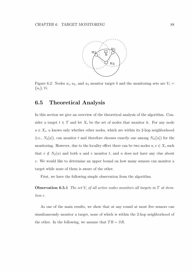
CHAPTER 6. TARGET MONITORING 88
b
u3
u2
u1
Figure 6.2: Nodes u1, u2, and u3 monitor target b and the monitoring sets are Vi =ui, ∀i.
6.5 Theoretical Analysis
In this section we give an overview of the theoretical analysis of the algorithm. Con-
sider a target t ∈ T and let Xt be the set of nodes that monitor it. For any node
u ∈ Xt, u knows only whether other nodes, which are within its 2-hop neighborhood
(i.e., N2[u]), can monitor t and therefore chooses exactly one among N2([u]) for the
monitoring. However, due to the locality effect there can be two nodes u, v ∈ Xt such
that v /∈ N2(u) and both u and v monitor t, and u does not have any clue about
v. We would like to determine an upper bound on how many sensors can monitor a
target while none of them is aware of the other.
First, we have the following simple observation from the algorithm.
Observation 6.5.1 The set Vi of all active nodes monitors all targets in T at itera-
tion i.
As one of the main results, we show that at any round at most five sensors can
simultaneously monitor a target, none of which is within the 2-hop neighborhood of
the other. In the following, we assume that TR = SR.

CHAPTER 6. TARGET MONITORING 89
u3
u4
u5
u1
u2
Figure 6.3: For a target in the striped region (intersection of the five disks) we set asactive at most five nodes whereas only one node suffices.
Lemma 6.5.2 For any target t ∈ T , at most five nodes are set as active.
Proof Assume Xt to be the set of nodes that monitors a target t ∈ T in some
iteration. Suppose for the sake of contradiction that |Xt| > 5 and no two nodes
u, v ∈ Xt are within the 2-hop neighborhood of the other. As t is monitored by all
nodes in Xt, the Euclidean distance between t and any node w ∈ Xt must be at most
SR. Consider a disk D centered at t with radius equal to SR. All the nodes in Xt
must be within the disk D. Since |Xt| > 5 and nodes of Xt are in D, there will be at
least two nodes u′, v′ ∈ Xt whose Euclidean distance must be smaller than TR (we
consider TR the radius of D instead of SR, since SR = TR). Then u′ and v′ are
direct neighbors to each other, a contradiction.

CHAPTER 6. TARGET MONITORING 90
Input: A UDG G = (V, E) and a set of targets T such that each target ismonitored by at least one node.Output: A family of subsets of nodes V1, · · · , Vs such that each Vi monitors alltargets in T .1: i = 12: Broadcast pi(u) and T (u) to v ∈ N2(u)3: Receive pi(v) and T (v) from v ∈ N2(u)4: Compute Ta(u) = a|a ∈ T (u) ∩ T (v), v ∈ N2(u), ∀a ∈ T (u)5: /*Ta(u) represents the set of nodes that monitor a*/6: For each round i7: Compute rank r(Ta(u)), ∀a ∈ T (u)8: If ∃a ∈ T (u) such that9: r(Ta(u)) < r(Ta(v)), v ∈ N2(u) Then10: /*Selects the smallest ranked node for each target*/11: u becomes active12: Endif13: i = i + 114: If u is active Then15: cti(u) = cti−1(u) + 116: Endif17: If cti(u) 6= cti−1(u) Then18: Send pi(u) to v ∈ N2(u)19: Endif20: Receive pi(v) from v ∈ N2(u)21: Endfor
Figure 6.4: A 2-local algorithm for the target monitoring problem.
A tight example of the above lemma is shown in Figure 6.3, where five nodes are
put on the vertices of a regular pentagon with side TR+ ε. They can all monitor any
target t in the striped region S which is the intersection of their respective sensing
disks. Note that for any ui, ui /∈ N2[uj] (i 6= j and i, j ∈ 1, 2, 3, 4, 5).
Then we derive the corollary from the above lemma.
Corollary 6.5.3 If V ∗i denotes the minimum set of nodes monitoring targets at it-
eration i, then |Vi| ≤ 5m ≤ 5|V ∗i |, where m = |T | is the number of targets given and

CHAPTER 6. TARGET MONITORING 91
|V ∗i | ≤ m.
Here we assume that in at each iteration i, we compare the size of the returned
monitoring set Vi by our algorithm to the minimum (optimal) sized monitoring set
V ∗i of the same iteration.
Now we show how the algorithm performs towards maximizing the value of z =
s/k. First we need some notation. Let X1, X2, · · · , Xm be subsets of sensors (Xi ⊆ V ,
1 ≤ i ≤ m) that monitor the targets t1, t2, · · · , tm, respectively. Let Xp be the
minimum cardinality subset among all Xi’s (ties are broken arbitrarily).
We divide each Xi (the nodes in Xi monitor target i) in the following way. Due
to the locality effect we can have at most five subsets Xi(i1), Xi(i2), Xi(i3), Xi(i4),
and Xi(i5) of Xi (i.e., Xi(ia) ⊆ Xi, 1 ≤ a ≤ 5, 1 ≤ i ≤ m) such that no node
in one subset knows whether any nodes in other subsets are monitoring i. In other
words, there is no node u ∈ Xi(ia) such that v ∈ Xi(ib), a 6= b and v ∈ N2[u]. Let
X∗=min1≤i≤m,1≤a≤5|Xi(ia)|. Note that X∗ ≥ 1.
Denote by zopt the optimal value of z and zopt > 0, that is, zopt ≥ z = s/k for all
possible values of s and k. If zalg denotes the value of z obtained by our algorithm
then we have the following lemma:
Lemma 6.5.4 zopt ≤ |Xp| and zalg ≥ |Xp|/5. Hence zalg ≥ |Xp|/5 ≥ zopt/5.
Proof First we derive the value of zopt. In order to compute the value zopt, notice
that there can be at most |Xp| monitoring sets V1, V2, · · · , V|Xp| such that each node
in Xp can participate in these monitoring sets exactly once. It is easy to see that for
the optimal algorithm to generate the |Xp| + 1-st monitoring set, V|Xp|+1, there will
be at least one node in Xp such that the number of participations of that node in

CHAPTER 6. TARGET MONITORING 92
V1, V2, · · · , V|Xp|, V|Xp|+1 is at least two (because of the Pigeonhole Principle). Thus
zopt ≤ s/k ≤ |Xp|, where s ≤ |Xp| (i.e., at most |Xp| monitoring sets V1, V2, · · · , V|Xp|)
and k = 1.
We now analyze the behavior of the algorithm to find zalg. With each node
participating exactly once, the algorithm can generate at least |Xp|/5 monitoring sets
V1, V2, · · · , V|Xp|/5. Hence zalg ≥ |Xp|/5 ≥ zopt/5.
6.5.1 TR = 2 ∗ SR
In this section we assume that the transmission range of a sensor is twice its sensing
range, TR = 2∗SR. In the previous subsection it is shown that we can achieve a good
approximation factor (a constant factor) for the size of each of the monitoring sets.
However, when the number of targets is a constant, the approximation factor is much
worse towards minimizing the value of k. This is because of the limited information
of the 2-hop neighborhood available to individual sensors and we assumed that the
transmission range is equal to the sensing range of a sensor. Here we investigate
whether the value of k can be improved by assuming TR = 2 ∗ SR. This is a
reasonable assumption in the context of coverage (monitoring) problems in WSNs
[25]. However, we use this assumption and obtain some useful insights into the target
monitoring problem.
Observation 6.5.5 Let node u ∈ V monitor T (u) ⊆ T targets. If there is a node
v ∈ V , v 6= u, such that T (u) ∩ T (v) 6= φ, then v ∈ N(u).
Proof Suppose for the sake of contradiction that v /∈ N(u). Since T (u) ∩ T (v) 6= φ,
that means v can monitor a target which u can monitor. In this case the Euclidean
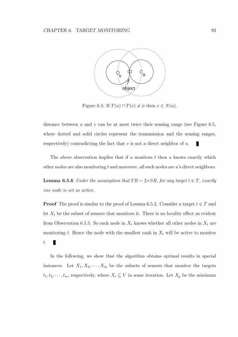
CHAPTER 6. TARGET MONITORING 93
v u
object
Figure 6.5: If T (u) ∩ T (v) 6= φ then v ∈ N(u).
distance between u and v can be at most twice their sensing range (see Figure 6.5,
where dotted and solid circles represent the transmission and the sensing ranges,
respectively) contradicting the fact that v is not a direct neighbor of u.
The above observation implies that if u monitors t then u knows exactly which
other nodes are also monitoring t and moreover, all such nodes are u’s direct neighbors.
Lemma 6.5.6 Under the assumption that TR = 2∗SR, for any target t ∈ T , exactly
one node is set as active.
Proof The proof is similar to the proof of Lemma 6.5.2. Consider a target t ∈ T and
let Xt be the subset of sensors that monitors it. There is no locality effect as evident
from Observation 6.5.5. So each node in Xt knows whether all other nodes in Xt are
monitoring t. Hence the node with the smallest rank in Xt will be active to monitor
t.
In the following, we show that the algorithm obtains optimal results in special
instances. Let X1, X2, · · · , Xm be the subsets of sensors that monitor the targets
t1, t2, · · · , tm, respectively, where Xi ⊆ V in some iteration. Let Xp be the minimum
CHAPTER 6. TARGET MONITORING 94
cardinality subset among all Xi’s (ties are broken arbitrarily). If Xi ∩ Xj = φ, i 6= j
and 1 ≤ i, j ≤ m, that is, a sensor monitors exactly one target, then we have the
following lemma.
Lemma 6.5.7 With the above assumption and TR = 2 ∗ SR, we have zalg = zopt.
Proof Let Xp = u1, u2, · · · , u|Xp| denote the subset of sensors that monitor p (recall
that Xp has minimum cardinality among |Xi|’s). The optimal algorithm can produce
at most |Xp| monitoring sets V1, V2, · · ·V|Xp| with each node in Xp participating exactly
once. Since Xp has the smallest cardinality, for the optimal algorithm to produce the
next monitoring set V|Xp|+1, at least one of the nodes in Xp must be selected in V|Xp|+1.
So, zopt = |Xp|/1 ≥ (|Xp| + 1)/2.
We see how the algorithm behaves towards finding zalg. Since there is no locality
effect (all nodes u1, u2, · · · , u|Xp| are aware of each other about monitoring p), the
algorithm sets as active exactly one node from Xp (say node uj is selected in some
iteration). Since Xp ∩ Xi = φ, for i 6= p and 1 ≤ i ≤ m, no other nodes from Xp will
be selected (active) in that iteration. Therefore, at any iteration exactly one node is
set as active from Xp and hence we have V1, V2, · · ·V|Xp| monitoring sets.
Now we show that any node uj ∈ Xp is exactly used once in V1, V2, · · ·V|Xp|
monitoring sets.
Suppose for contradiction that a node uj is used in monitoring sets Vr and Vw,
where 1 ≤ r, w ≤ |Xp| and r < w. After being selected first in Vr, uj’s ct(uj) value
is increased by one. If uj is selected (from Xp) again in Vw, that means its rank is
smaller than other nodes in Xp. Since w ≤ |Xp| and exactly one node is selected
from Xp, there is at least some node in Xp which has not been selected in previous

CHAPTER 6. TARGET MONITORING 95
monitoring sets V1, V2, · · · , Vw′<w. If this has not been selected in previous monitoring
sets its rank will be smaller than uj’s, a contradiction. The claim follows.
6.6 Simulations
We conduct extensive simulations on randomly generated UDGs to study the per-
formance of the proposed 2-local algorithm. In this section, experimental results
are presented regarding (i) maximizing z = s/k and (ii) the sizes of monitoring sets
V1, V2, · · · , Vs. In the experiments, first we distribute a set of m ∈ 10, 20, 30, 40, 50
targets randomly and uniformly in a square field of size 400m x 400m. Thereafter,
a set of n ∈ 100, 200, 300, 400, 500 nodes is generated (uniformly and randomly) in
the plane from which a UDG is formed. The algorithm then constructs monitoring
sets for the targets.
6.6.1 Experimental Results
Experiments are done using our own simulator in Java. Setting both the transmission
and the sensing range to 60m for all nodes, we apply the algorithm in a 400m x 400m
square with n = 100, m = 10 and first compute the minimum cardinality set Xp.
Recall that given t1, t2, · · · , tm targets, Xp is the minimum cardinality set among
X1, X2, · · · , Xm, where Xi ⊆ V denotes the set of nodes that monitors the target ti,
(1 ≤ i ≤ m). Then the monitoring sets V1, V2, · · · , V|Xp| are generated.
In the experiments, we set the optimal value of z, zopt = s/k = |Xp|/1, since the
optimal algorithm can generate at most |Xp| monitoring sets with k = 1. In order
to find the value of zalg, we figure out the maximum frequency k of a node in Xp in

CHAPTER 6. TARGET MONITORING 96
10 20 30 40 501.5
2
2.5
3
3.5
4
4.5
5
5.5
# of Targets(a)
Val
ue o
f z
Opt zAlg z
10 20 30 40 503
3.54
4.55
5.56
6.57
7.58
8.59
9.51010
# of Targets(b)
Val
ue o
f z
Opt zAlg z
10 20 30 40 505
5.5
6
6.5
7
7.5
8
8.5
9
9.5
10
10.5
# of Targets(c)
Val
ue o
f z
Opt zAlg z
10 20 30 40 506
6.57
7.58
8.59
9.510
10.511
11.51212
# of Targets(d)
Val
ue o
f z
Opt zAlg z
10 20 30 40 50
99.510
10.511
11.512
12.513
13.514
14.515
15.51616
# of Targets(e)
Val
ue o
f z
Opt zAlg z
Figure 6.6: Average z values (optimal zopt values by solid lines and zalg by dashedlines) for (a) 100 (b) 200 (c) 300 (d) and (e) 500 sensors.
these monitoring sets and obtain zalg = |Xp|/k. After generating 100 random graphs
successively with the same number (m = 10) of targets, the size of the minimum
cardinality set |Xp| and the maximum frequency k of a node in the monitoring sets
are obtained. Hence zopt and zalg for each graph are computed. Finally the average
values of zopt and zalg are determined.
Keeping m = 10, we increment the value of n by 100 each time and repeat
the whole procedure until n = 500. In this way, we obtain the average values of
the parameters (zopt and zalg) for each value of n. Thereafter, for each value of
m ∈ 20, 30, 40, 50 and for each value of n = 200, 300, 400, 500, the experiment is
run 100 times and the averages of zopt and zalg are determined.
The results are plotted in Figure 6.6, where the x-axis shows the number of targets
in the field and the y-axis represents the average values of zopt and zalg. Optimal values

CHAPTER 6. TARGET MONITORING 97
zopt are shown in solid lines and the values zalg by the algorithm are shown in dashed
lines. In these average graphs the experimental results found are much better than
the theoretical bounds established in Lemma 6.5.7. Note that the average zalg values
are within a small constant (at most 3) of the optimal average zopt values. As is
obvious from the figures the results are even better and consistent in dense graphs
(we assume, having 500 sensors in a square of 400m x 400m is denser than having
100 or 200 sensors in the same field). This is intuitive because having more sensors
in small a area reduces the locality effect and sensors are likely to be aware of other
sensors monitoring the same object.
Finally, as a by product of the algorithm we also consider the sizes of individual
monitoring sets. We compute the cardinality of each monitoring set Vi and compare
it with the optimal size of the monitoring set V ∗i . To find the optimal value |V ∗
i |, we
have used the number of targets as the value of |V ∗i |, that is, |V ∗
i | = m. We compute
the size of each monitoring set Vi generated by the algorithm and find that on average
it is 3.16 times the size of V ∗i .
In previous figures, we have shown the average zalg values for different number of
sensors and targets. In Figure 6.7, we plot standard deviations of zalg to see how the
values deviate from the average zalg. The smaller standard deviations (less than 0.7)
for all values of n are an indication that most zalg’s tend towards the mean. For large
n, the standard deviation seems to be lower than that of smaller n. This is because
the locality effect, in general, is much less for a large number of sensors distributed
in a relatively smaller area.
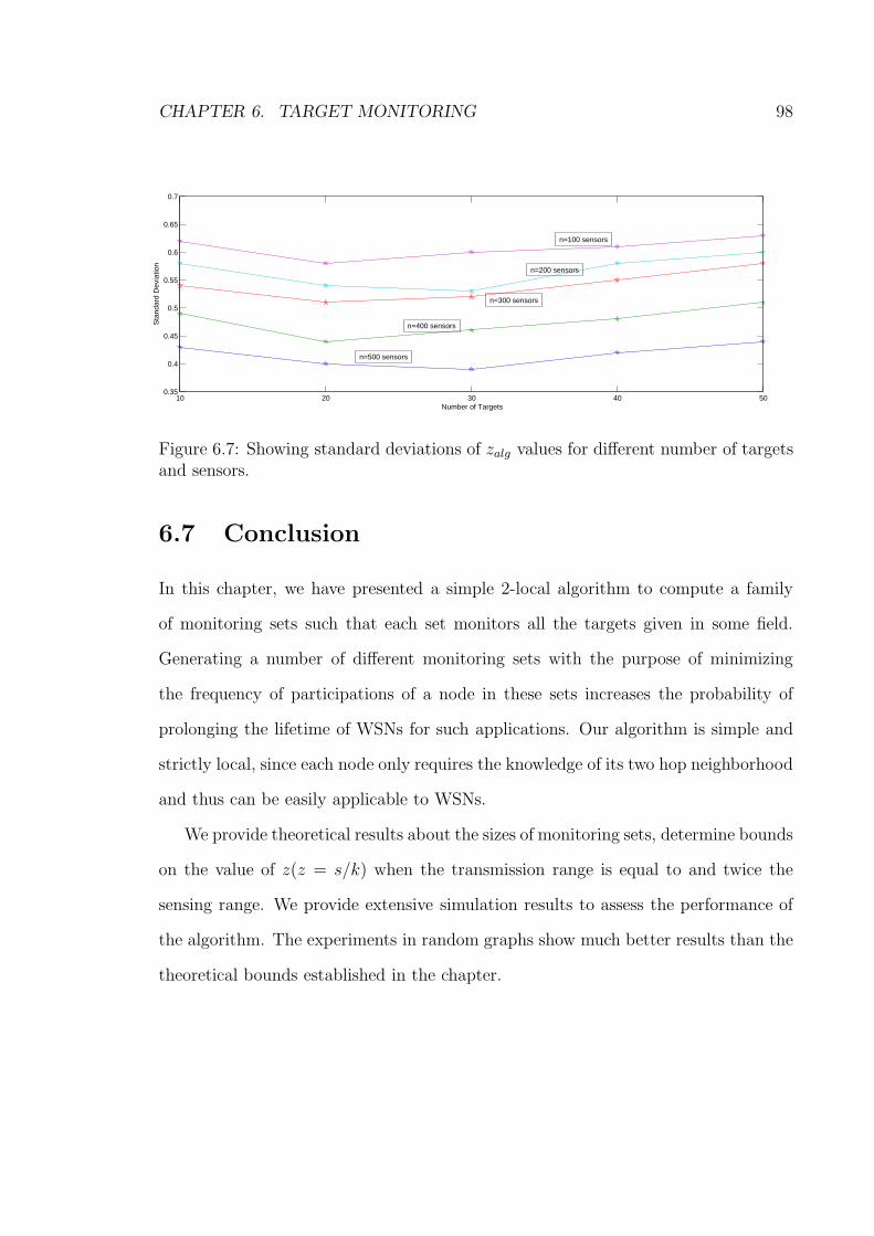
CHAPTER 6. TARGET MONITORING 98
10 20 30 40 500.35
0.4
0.45
0.5
0.55
0.6
0.65
0.7
Number of Targets
Sta
ndar
d D
evia
tion
n=500 sensors
n=400 sensors
n=300 sensors
n=200 sensors
n=100 sensors
Figure 6.7: Showing standard deviations of zalg values for different number of targetsand sensors.
6.7 Conclusion
In this chapter, we have presented a simple 2-local algorithm to compute a family
of monitoring sets such that each set monitors all the targets given in some field.
Generating a number of different monitoring sets with the purpose of minimizing
the frequency of participations of a node in these sets increases the probability of
prolonging the lifetime of WSNs for such applications. Our algorithm is simple and
strictly local, since each node only requires the knowledge of its two hop neighborhood
and thus can be easily applicable to WSNs.
We provide theoretical results about the sizes of monitoring sets, determine bounds
on the value of z(z = s/k) when the transmission range is equal to and twice the
sensing range. We provide extensive simulation results to assess the performance of
the algorithm. The experiments in random graphs show much better results than the
theoretical bounds established in the chapter.

Chapter 7
Self Protection
Since sensors provide monitoring to targets, it is often necessary to give them a level
of protection such that sensors can take certain actions when they are themselves the
subject of attacks. One natural idea is to monitor sensors by their neighbors such that
these neighbors can inform the base station when monitoring sensors malfunction or
are in danger.
Keeping this in mind, the p-self-protection subset problem has been formally intro-
duced in [79]. The p-self-protection subset problem is defined to be a subset of sensors
such that for any sensor in the network there are at least p active sensors from the
subset that monitor it. In this chapter, we study the p-self-protection subset problem.
The authors in [79] first show that finding a minimum 1-self-protection subset
is NP-hard and then give an O(log n)-approximation algorithm. Later, with a view
to obtaining a constant factor approximation ratio, centralized and distributed al-
gorithms to solve the general p-self-protection subset problem are presented in [77].
Here, first we present a counterexample showing that the algorithm in [77] fails to
find a p-self-protection subset in the network. Thereafter a distributed algorithm
99

CHAPTER 7. SELF PROTECTION 100
for the p-self-protection subset problem is given which achieves a constant factor ap-
proximation ratio. To the best of our knowledge, this is the first constant factor
approximation ratio to the p-self-protection subset problem. The distributed algo-
rithm runs in O(log∗ n) time, where n is the total number of sensors in the network.
7.1 Introduction
As pointed out earlier, once deployed with a limited amount of energy, nodes in
sensor networks continue to spend energy by sensing, gathering, and distributing
data from the environment. Among myriad of applications, sensor networks are
used for protection and surveillance of many different environments such as museum
monitoring, military surveillance, target tracking, and so on. More specifically, nodes
carry out protection and monitoring activities by collecting and sending timely signals
to a base station to take appropriate measures in case some unusual events occur to
the targets they monitor.
Although sensors are often used for protection of targets as mentioned, there are
situations when it is vital to monitor the sensors as well. The issue of monitoring
sensors arises because battery-powered sensors are vulnerable to damage, failure and
attacks. If sensors themselves are incapable of performing monitoring, then how
could we protect targets (or objects, they are used interchangeably)? It is therefore
important to ensure that sensors are active and functioning as desired. One of the
ways this can be done is to require neighboring sensors to monitor the conditions of
each other.
Imagine a scenario where among the set of sensors there is a single sensor which is
monitoring a certain object. If, for some reason, this sensor malfunctions or runs out

CHAPTER 7. SELF PROTECTION 101
of energy then the object will be left unprotected. However, if there were some other
neighboring sensors which could monitor this particular sensor then any status of that
sensor (whether running out of energy or in danger) could be relayed by them to the
base station so that proper action could be taken. For example, the sensor may be
replaced by additional sensors, if it does not function properly. This scenario raises
the issue that sensors themselves require a certain level of protection. The problem
of protecting the sensors by other sensors is called self-protection. In its simplest
form, a sensor network is self-protected if all sensors are protected by at least one
active sensor (other than itself), where active sensors are sensors which monitor their
neighbors by being active. In general, a WSN is p-self-protected if at any moment for
any sensor there are at least p active sensors (other than itself) that can monitor it.
This problem has been formally introduced and investigated by Liu et. al [79].
The rest of the chapter is organized as follows. Section 7.2 describes related work.
In Section 7.3 we define the p-self-protection subset problem, show a counterexample
to the work in [77], and present a distributed algorithm to solve the problem. We
provide a theoretical analysis of our algorithm in Section 7.4 followed by simulation
results in Section 7.5. Conclusion is provided in Section 7.6.
7.2 Related Work
Since sensors are power-limited and monitoring requires sensors to be active all the
time thereby consuming valuable energy, finding a ‘small’ number of sensors to do
the monitoring has been one of the main objectives of research in this regard. This
small subset of active sensors are used to provide protection for every location of the
area, in which they are deployed, and at the same time other sensors can be put in

CHAPTER 7. SELF PROTECTION 102
the energy-efficient sleep mode to conserve energy. A number of coverage problems,
including protection of certain static objects with a required degree of fault-tolerance,
and methods to solve them have been surveyed by Wu et. al [10], where the main
focus is on the area coverage problem.
A generalization of the area coverage problem called the k-coverage, i.e., whether
every point is covered by at least k sensors, is studied by Kumar et el [43]. The
k-coverage problem is directly related to the fault-tolerance issue in WSNs. This is
because k-coverage basically provides fault-tolerance in the network since failure of
at most k′ < k monitoring nodes to monitor a particular area will not leave that area
uncovered. Gui et al [29] propose algorithms for area coverage problems considering
fault-tolerance, energy-consumption and quality of coverage.
A shift from the coverage problem to the problem of protecting the sensors them-
selves was first suggested by Liu et al [79]. In [79] the authors prove that finding
minimum 1-self-protection subset (that is, finding a subset of nodes of minimum car-
dinality such that each node in the network is protected by at least one other node)
is NP-complete through a reduction from the set-cover problem [26]. As a conse-
quence they give a centralized algorithm for this problem and achieve a 2(1 + log n)
approximation ratio, where n is the total number of sensors. That is, their algorithm
finds a 1-self-protection subset which is at most O(log n) times the cardinality of the
minimum 1-self-protection subset. However, they do not give any algorithm for the
general p-self-protection subset problem. The authors also show that focusing only
on the quality of area or object covering does not necessarily make the sensors to be
self-protected. Subsequently, a probabilistic definition of the self-protection subset (a

CHAPTER 7. SELF PROTECTION 103
protection is called the δ-p-self-protection if the probability that a node is not p-self-
protected is less than δ), as well as two randomized algorithms to solve the problem
in a distributed fashion, are given in [79].
Later, the problem of finding a minimum p-self-protection subset was thoroughly
studied along with some of its variants such as requiring that the protecting sen-
sors be also connected, allowing sensors with varying sensing ranges, and so on, by
Wang et. al [77]. In their paper, the authors claim that they have two constant fac-
tor approximation algorithms (in both centralized and distributed settings) for this
problem. Unfortunately, their claim is in error. We provide a counterexample to show
an instance of a graph where the p-self-protection algorithm does not form a subset
that p-protects the nodes in G. They discuss other variants of the problem, namely,
how p-self-protection can be achieved when the sensing radii of the sensors are not
the same, or generating a certain number of p-self-protection subsets and activating
them one after the other.
Here we investigate the p-self-protection problem. By presenting a counterexample
of the work of Wang et. al [77], we provide a distributed algorithm to solve the
p-self-protection problem. To the best of our knowledge this is the first distributed
constant factor approximation algorithm for the p-self-protection problem. This result
is significant in two ways: first, it achieves a constant factor which is better than the
previous (logarithmic factor) results and second, it is distributed. The earlier version
of the algorithm appeared in [34].

CHAPTER 7. SELF PROTECTION 104
7.3 Minimum p-self-protection Subset Problem
As mentioned before, a WSN is p-self-protected if, for any sensor, there are at least
p neighboring active sensors (a sensor is not a neighbor to itself) that monitor it.
When the network is modeled as a UDG, G = (V, E), the minimum p-self-protection
subset [77] is defined as a subset P ⊆ V such that the network is p-self-protected and
the cardinality of P is minimized. See Figure 7.1, where the set of black nodes form
a 1-self-protection (Figure 7.1 (a)) and a 2-self-protection (Figure 7.1 (b)) subsets.
As mentioned before, it is proved in [79] that computing a minimum 1-self-protection
subset is NP-hard, which implies that the general minimum p-self-protection subset is
also NP-hard. From now on instead of using ‘p-self-protection’ we use ‘p-protection’.
(b) 2−self−protected(a) 1−self−protected
Figure 7.1: Minimum 1-self-protection and 2-self-protection subsets.
In the following, after describing the algorithm of Wang et. el, we present a
counterexample which makes the p-protection algorithm fail to find a p-protection
subset.

CHAPTER 7. SELF PROTECTION 105
7.3.1 Wang et. al [77] Algorithm: p-protection Subset Prob-
lem
The algorithm in [77] for the general minimum p-protection subset problem is now
described. In the first iteration (k = 1), the algorithm [77] first finds an MIS M1
based on the ranks (each node u is assigned a unique integer from [1, n] called its
rank, r(u)) of the nodes, where a node in selected to be in M1 if it has the largest
rank among all its neighbors. After M1 is formed, each node not selected in M1 is
then assigned a unique rank r(v) = r(v) + k ∗ n, where initially k is assigned 1 and
incremented by one at each iteration, and the ranks of the nodes belonging to that
MIS are not changed. Then in the next iteration(k = 2), the algorithm generates a
new MIS M2 from the nodes not selected in M1 based on their ranks.
Thereafter, in the 3rd iteration, ranks are updated by the equation r(v) = r(v) +
3∗n for those nodes which did not belong to M1 and M2 and a new MIS M3 is formed.
This procedure of generating new MISs is repeated p times, and it is claimed that
this algorithm finds p MISs. Finally, as this algorithm continues, if a node u ∈ Mi,
1 ≤ i ≤ p has fewer than p neighboring nodes in⋃p
i=1 Mi, then u randomly selects
a neighbor v /∈ ⋃pi=1 Mi to protect u to such that u becomes p-protected. According
to [77], the union of all Mi’s and the selected neighbors form the desired p-protection
subset.
In order to prove this claim (Theorem 2 in [77]), it is stated that for any node
u ∈ ⋃pi=1 Mi, u has at least p− 1 protectors from
⋃pi=1 Mi since it has been protected
by MIS nodes in every iteration except the iteration in which it is selected. Then if
u has only p − 1 neighboring nodes in⋃p
i=1 Mi, it just selects an arbitrary neighbor
v, which did not belong to any of the Mi’s, to protect itself.

CHAPTER 7. SELF PROTECTION 106
4
12 3 31
4
21
Figure 7.2: Counterexample to the proof of Theorem 2 [77].
However, this statement is not correct. Figure 7.2 shows a counterexample for the
p-protection subset problem, where p = 4. Assume that the algorithm finds the first
MIS M1 consisting of nodes shown with label 1. According to the algorithm, another
MIS M2 can be found consisting of the nodes that do not belong to M1. However,
in the example, there is no way to form a second MIS M2 from the remaining nodes
V \ M1 because any attempt to construct the second MIS without using nodes from
the previous MIS will fail.
More specifically, if we want to form the second, the third or the fourth MISs M2,
M3 or M4, each will consist of exactly two nodes (shown with label 2, label 3, and
label 4, respectively) and none of which is an MIS of the whole graph. This means
that in any case, either the middle label 1 node (when we form M2 and M4) or the
label 1 nodes on the left and on the right (for M3) are not protected by any nodes.
Furthermore, according to [77], for all nodes u ∈ ⋃pi=1 Mi, u must have at least p− 1
protectors from⋃p
i=1 Mi, given that u has already been protected by MIS nodes in
every iteration except the iteration in which it is selected as a node in MIS. However,
in the example of Figure 7.2, the middle label 1 node is not protected by p − 1 = 3
nodes. The authors of the paper [77] agreed that the counterexample we provide is
correct [73].

CHAPTER 7. SELF PROTECTION 107
7.3.2 Solution: 1-protection Subset Problem
For the minimum 1-protection subset problem we present a distributed algorithm that
gives a constant approximation ratio. Basically our algorithm is almost the same of
[77]. However, we give a different proof for the approximation factor. First, nodes
distributedly construct an MIS, S (following the algorithm in [66]). Thereafter, each
node in S arbitrarily selects one of its neighbors to protect it. Let the set of selected
nodes be denoted as S ′. All nodes in S ∪ S ′ are set as active. Let the set of active
nodes be denoted by A1. We claim that A1 forms a valid 1-protection subset. Let
A∗1 denote the minimum 1-protection subset. The constant approximation ratio is
obtained as follows.
Theorem 7.3.1 For the minimum 1-protection subset problem, the distributed algo-
rithm finds a valid 1-protection subset A1 and has size at most 10 times the minimum
1-protection subset A∗1, that is, |A1| ≤ 10|A∗
1|.
Proof First, we show that A1 provides 1-protection to the nodes in G. Notice that
A1 = S ∪ S ′. Consider any node u. If u /∈ S then it must have a neighbor from
S. This is because S is an MIS. So u is 1-protected by some nodes in S. Secondly,
if u ∈ S then it does not have any neighbor that is in S. However, it chooses an
arbitrary neighbor from u′ ∈ N(u) to protect itself. Therefore, u is protected by the
node it selects.
Each node in S selects an arbitrary node, so we have |A1| ≤ 2|S|. In order to form
the minimum 1-protection set A∗1, the optimal algorithm must provide 1-protection to
the nodes in S. Since any node /∈ S can have at most 5 S nodes in its neighborhood,
the optimal algorithm must choose at least one node to provide 1-protection to at
most 5 S nodes. So, |A∗1| ≥ |S|
5≥ |A1|
2∗5= |A1|
10and the claim follows.

CHAPTER 7. SELF PROTECTION 108
It is intersting to note that a CDS is also a 1-self protection subset unless the CDS
is a singleton.
7.3.3 Distributed Algorithm D: p > 1-protection Subset Prob-
lems
In this section, we present a distributed algorithm for the general p-protection subset
problem, where p > 1. Let Ap and A∗p denote the p-protection subset produced by
the algorithm and the minimum p-protection subset, respectively.
p-protection
First, run the distributed MIS [66] algorithm on G and let S be the set of nodes
returned by the algorithm, that is, S is an MIS in G. Nodes in S are set as active.
Let N q(u) denote a set of at most q nodes selected by a node u from its neighborhood,
N q(u) ⊆ N(u). We take advantage of a well-known property of UDGs towards finding
p-protection subset. In a UDG, a node u requires a set N 5(u) to protect all nodes
in v ∈ N(u) \ N 5(u). Specifically, for any node v ∈ N(u) \ N 5(u) 6= φ, there exists
a node w ∈ N5(u) such that vw ∈ E. We informally describe the algorithm in the
following:
Consider a node u ∈ S. It provides 1-protection to its neighbors N(u). Then it
finds a subset N5p(u) to provide the required p-protection to nodes N [u]. We need
a little explanation of why we choose N 5p(u) nodes to provide p-protection to nodes
N [u]. First note that by selecting N 5p(u), u becomes at least p-protected, since
|N(u)| ≥ |N5p(u)| ≥ p. Second, the nodes N(u) \ N 5p(u) are guaranteed to have
at least p-protection. Also each node u′ ∈ N5p(u) in the selected node set N 5p(u) is

CHAPTER 7. SELF PROTECTION 109
Algorithm D for p-protection subsetInput: An undirected graph G and an integer parameter pOutput: Protection set Ap
1: Run Distributed MIS Algorithm [66]2: Let S be the MIS found3: If u ∈ S4: If p = 15: Select v ∈ N(u) to protect u6: Set u and v active7: Endif8: If p ≥ 29: Select a set N 5p of at most 5p nodes
//N5p provides protection to nodes in N [u]10: Set N5p ∪ u as active11: EndIf12: EndIf //All active nodes form the p-protection subset Ap.
Figure 7.3: Algorithm D for the p-protection subset.
provided at least p−1-protection by the nodes u′′ ∈ N5p(u), u′ 6= u′′. Since u provides
protection to u′, u is at least p-protected. Therefore, in order to guarantee full p-
protection to all nodes N [u], u selects N 5p(u). Let S ′ represent the set of selected
nodes.
All nodes Ap = S ∪ S ′ in the graph are set as active and they constitute the solu-
tion of the p− protection subset problem. In Figure 7.3, we present the distributed
algorithm D for the p-protection algorithm that is executed at each node u.
7.4 Theoretical Properties of Algorithm D
In this section we provide the correctness of the algorithm, that is, we prove that the
algorithm produces a p-protection subset for all the nodes in the underlying graph.

CHAPTER 7. SELF PROTECTION 110
Lemma 7.4.1 Active nodes in G constitute a p-protection subset to the nodes in G.
Proof Consider a node u ∈ V . Then we have the following three cases:
Case 1: Node u is not active. Then it must have a neighbor u′ ∈ S. Since u′
selects N5p(u′) to provide protection to its neighbors, u ∈ N(u′) must have at least
p active nodes protecting it. In fact, u is at least p + 1 protected since it is also
protected by u′.
Case 2: Node u is active and u ∈ S ′. Then it must have a neighbor node u′ ∈ S
and u ∈ N5p(u′). Therefore, u gets protected by at least p − 1 nodes from N 5p(u′).
However, u is at least p-protected since its neighbor u′ also protects u.
Case 3: Node is active and u ∈ S. Since u selects a subset N 5p(u′) of at most
5p neighbors to provide p-protection to its neighbors, u is at least p-protected (recall
that |N(u)| ≥ p).
In the following we prove the main result of this chapter.
Theorem 7.4.2 The size of the set Ap (p > 1) returned by the algorithm is at most
25 + 5p
times the optimum solution A∗p.
Proof According to the algorithm, each node u ∈ S selects a subset N 5p(u) of at most
5p nodes in its neighborhood to provide the required p-protection to its neighbors.
Recall that a node u′ ∈ V \ S can have at most 5 S nodes in its neighborhood, that
is, |N(u′) ∩ S| ≤ 5. Since each of these 5 nodes can select at most 5p nodes, we have
|Ap| ≤ |S| + 5p|S| = (5p + 1)|S|.
In order to form the minimum p-protection set A∗p, the optimal algorithm must
provide p-protection to the nodes in S. Since a node /∈ S can have at most 5 S nodes
CHAPTER 7. SELF PROTECTION 111
in its neighborhood, the optimal algorithm must select at least p nodes to provide
p-protection to at most 5 S nodes. Therefore,
|A∗p| ≥ p
|S|5
|A∗p| ≥ p
|Ap|5(5p + 1)
≥ p|Ap|
25p + 5
|Ap| ≤ (25 +5
p)|A∗
p|
7.4.1 Time and Message Complexities
According to our model LOCALS, exchanging indices and degrees with direct neigh-
bors can be done in a constant time [61]. Line 1 in the algorithm D constructs a
distributed MIS [66] in a UDG which requires O(log∗ n) time [66], where n is the
number of nodes in G. The algorithm in [66] can be applied to any growth bounded
graph, where growth boundedness means that there is a constant number of inde-
pendent nodes in some fixed hop neighborhood. Lines 2-12 of algorithm D can be
executed in constant time since nodes only perform local computation [61] in their
constant hop neighborhood. Thus algorithm D needs O(log∗ n) time.
Each node broadcasts a single message containing its index and degree to its direct
neighbors. As mentioned in [66], the algorithm for generating an MIS requires at most
O(|E| log∗ n) messages. Also nodes in S inform their selected neighbors to become
active by sending them a message which totals at most O(n) messages. Thus the
message complexity of algorithm D is O(|E| log∗ n).
This suggests the following theorem:

CHAPTER 7. SELF PROTECTION 112
Theorem 7.4.3 For UDGs, the p-protection subset problem can be solved within a
constant factor of the optimum, in O(log∗ n) time and O(|E| ∗ log∗ n) messages.
7.5 Simulations
We conducted extensive simulations on random UDGs to study the performance of
our p-protection algorithm. In this section, we provide and analyze experimental
results and show how the results differ from optimality. Specifically, we carry out
the experiments for p = 1, 2 and 3. By placing nodes uniformly and randomly in the
plane, we constructed the UDGs. If the underlying graphs are connected we apply
the algorithm to construct p-protection subsets.
7.5.1 Experimental Setup
Experiments are done using our own simulator in Java. In the simulation, we have
chosen a square field of size 500m x 500m, where n ∈ 100, 200, 300, 400, 500 nodes
are distributed. The transmission range of all nodes is set to 60m. For each value
of n, we generate 100 different randomly connected topologies. For each value of n
and each topology we run the algorithm which generates p = 1, 2 and 3-protection
subsets for the topology.
7.5.2 Experimental Results
After generating a connected random topology with n = 100, we apply the algorithm
and compute the sizes of p-protection subsets for p ∈ 1, 2, 3. Then we generate 100
such random topologies successively and for each such graph the sizes of p-protection

CHAPTER 7. SELF PROTECTION 113
subsets are computed. Finally, we obtain the average size of each of the p-protection
subsets of all the 100 topologies. The value of n is then incremented by 100 (i.e.,
n = 200) and the whole procedure is repeated. We continue incrementing the value
of n by 100 each time and repeating the experiment until n = 500.
The results are plotted in Figure 7.4, where the x-axis shows the number of
nodes in the generated topology and the y-axis represents the average sizes of p-
protection subsets (average sizes of the 1-protection subsets are shown by the solid
line, 2-protection by the dashed line and 3-protection by the dotted line). For the
1-protection subset, the average sizes remain more or less stable for different values
of n. As can be seen from the graph, average sizes for 2 and 3-protection subsets
increase for larger values of n. In the following, we explain the behavior of the curves.
The reason of the increase of sizes of 2 and 3-protection subsets is given below.
Given a constant transmission radius for the nodes and fixed field size, for smaller
values of n (100, or 200) a node in a random topology has a smaller size neighborhood
than for larger values of n (400 or more). Thus in the case of smaller values of n,
where the neighborhood of a node is smaller, the probability that two or more nearby
MIS nodes select the same node is relatively high. Similarly for larger values of n,
when the neighborhood of a node increases the probability that two or more nearby
MIS nodes select the same nodes is lower because there are lots of other nodes to
choose from (a node’s neighborhood). That is why, the number of nodes selected
by the MIS nodes increases for higher values of n. However, we see a sharp rise in
the number of active nodes constituting 2 and 3-protection subsets than that of 1-
protection subset. This is because the number of nodes selected by an MIS node in
2 and 3-protection subsets is at most 15 and 20, respectively (which is exactly 1 for

CHAPTER 7. SELF PROTECTION 114
the 1-protection subset).
In Figure 7.5, we show the average approximation ratios generated for p-protection
subsets for different values of n. We determine the approximation ratios by comparing
the sizes of p-protection subsets generated by the algorithm with the lower bound on
the corresponding sizes by the optimal algorithm (given in Theorem 7.4.2). Following
the argument given in the previous paragraph, we find that the approximation ratios
for the 1-protection subset remains stable around 7 for all values of n, whereas the
approximation ratios for 2- and 3-protection subsets increase for larger values of n.
100 150 200 250 300 350 400 450 50020
40
60
80
100
120
140
160
180
Number of Sensors
Num
ber
of A
ctiv
e S
enso
rs
p=1p=2p=3
Figure 7.4: Showing average sizes of p-protection subsets for different values of n ∈100, 200, · · · , 500 and p ∈ 1, 2, 3.
As before, we compute standard deviations of the sizes of p-protection subsets
(p ∈ 1, 2, 3) to assess the performance of the algorithm. Figure 7.6 shows the
standard deviations of p-protection subsets. It can be observed that the data for
p-protection subsets tend not to vary a lot from the mean. However, we see a little
more variation in the obtained values for p = 2, 3 than p = 1. This is because for

CHAPTER 7. SELF PROTECTION 115
100 150 200 250 300 350 400 450 500
5.56
6.57
7.58
8.59
9.510
10.511
11.512
12.513
Number of Sensors
App
roxi
mat
ion
ratio
s
p=1p=2p=3
Figure 7.5: Showing average approximation ratios for p-protection subsets for differentvalues of n.
larger p’s the number of neighbors selected by the MIS nodes increases which, in turn,
increases the probability of obtaining a varying number of selected nodes for different
randomly generated graphs. Furthermore, with larger n this probability increases
even more which results in swelling the standard deviations.
7.6 Conclusion
Providing protection to sensors by their neighbors in a WSN is an interesting problem.
The need to protect sensors arises because they are vulnerable to attacks, failure or
damage while they monitor objects or provide coverage to a certain area. By having
some protector sensors around others allows us to know the status of these sensors and
take appropriate actions (replacing the dying and faulty sensors, if possible) in case
those sensing sensors fail or run out energy. In this chapter, we studied the problem
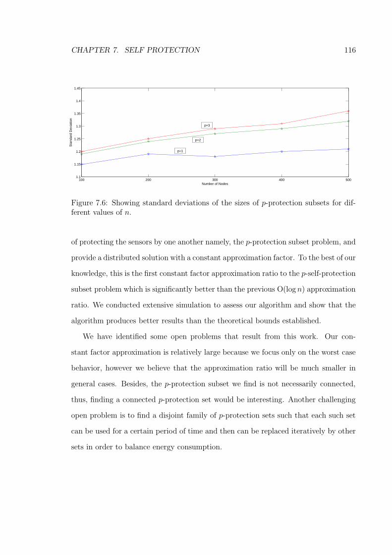
CHAPTER 7. SELF PROTECTION 116
100 200 300 400 5001.1
1.15
1.2
1.25
1.3
1.35
1.4
1.45
Number of Nodes
Sta
ndar
d D
evia
tion
p=1
p=2
p=3
Figure 7.6: Showing standard deviations of the sizes of p-protection subsets for dif-ferent values of n.
of protecting the sensors by one another namely, the p-protection subset problem, and
provide a distributed solution with a constant approximation factor. To the best of our
knowledge, this is the first constant factor approximation ratio to the p-self-protection
subset problem which is significantly better than the previous O(log n) approximation
ratio. We conducted extensive simulation to assess our algorithm and show that the
algorithm produces better results than the theoretical bounds established.
We have identified some open problems that result from this work. Our con-
stant factor approximation is relatively large because we focus only on the worst case
behavior, however we believe that the approximation ratio will be much smaller in
general cases. Besides, the p-protection subset we find is not necessarily connected,
thus, finding a connected p-protection set would be interesting. Another challenging
open problem is to find a disjoint family of p-protection sets such that each such set
can be used for a certain period of time and then can be replaced iteratively by other
sets in order to balance energy consumption.

Chapter 8
Topology Control
In previous chapters we mainly focus on finding subsets of nodes from the underlying
networks that are useful for different applications of WSNs. Here we are interested in
finding subsets of edges (instead of nodes) which allow various problems on WSNs to
be solved efficiently. Generally, topology control plays an important role in the design
of efficient algorithms for applications such as coverage, connectivity and routing in
WSNs [44, 45, 48, 75, 84, 50, 49, 63, 65, 64, 80, 81, 19, 32, 6]. The main idea is to
obtain a subgraph from the underlying network graph by removing some (possibly
redundant) edges in order to enhance the overall performance of the network in some
ways.
We present a local topology control algorithm (LTCA) in WSNs which has certain
desirable properties. First, the algorithm is very simple, strictly local (each node
requires only 1-hop information of its neighbors) and fast (requiring each node to
communicate with its neighbors exactly twice). Second, LTCA does not assume
the underlying graph to be a UDG, and in fact works on general connected graphs.
Third and the most important feature of LTCA is that it is completely independent
117
CHAPTER 8. TOPOLOGY CONTROL 118
of any location information of nodes; it relies only on the connectivity information
and the identities (ids) of the neighboring nodes. Assuming nodes are deployed in the
plane, it is shown that the resulting subgraph obtained by our algorithm is connected,
symmetric and contains few edge crossings. We provide simulation results which show
that on random graphs the resulting topology is a spanner and the average degree
of the subgraph is low. Due to the simplicity of the algorithm, LTCA can easily be
implemented in practical WSNs.
8.1 Introduction
In order to reduce the power consumption of the network and extend its lifetime,
topology control algorithms, in general, deal with finding a suitable structure (strictly
speaking, a spanning subgraph) of the given graph. This resulting subgraph is ex-
pected to have certain features (e.g., connectedness, planarity, sparseness, bounded-
degree, etc.) which facilitate, among other things, routing in the network. Given
a UDG G = (V, E), topology control algorithms focus on constructing a subgraph
G′ = (V, ETC), ETC ⊆ E. For transmission, longer links (edges and links are used in-
terchangeably) in the network consume more power than shorter links since the power
spent on a link for a transmission is directly proportional to at least the square of the
Euclidean length of that link. That is why, the general approach of topology control
algorithms is to remove longer links and retain shorter links which is supposed to save
energy in the long run for routing and thus help extend the lifetime of the network.
However, the disadvantage of this idea is that if too many longer links are eliminated
then some paths may be unacceptably longer in terms of the number of hops. This
increases the probability of message loss and takes longer to deliver messages. Care

CHAPTER 8. TOPOLOGY CONTROL 119
must be taken to design topology control algorithms to meet this challenge.
For any topology control algorithm, the first and foremost requirement is that the
subgraph G′ be connected. It is expected that G′ be symmetric, that is, for any two
nodes u and v, u is a neighbor of v if and only if v is a neighbor of u. Among other
properties, G′ should be planar (a graph is called a planar graph if no two edges in
G′ cross when drawn in the plane) because certain algorithms (for example, GPSR
[12]) utilize the planarity property of graphs for successful routing.
Another common requirement is that G′ be sparse; that is, the number of edges
should be in the order of the number of nodes. Sparsity of a graph helps maintain a
simple neighborhood for individual nodes. This is because the smaller the neighbor-
hood, the faster the information processing among the nodes in the neighborhood.
One of the important properties of G′ is that it should be a spanner. This means
that the cost of a shortest path between any two nodes in G′ must be at most t times
the cost of the shortest path between the same two nodes in G. There are a number
of cost metrics used in sensor networks. The most often used cost functions are the
Euclidean length of links, the Euclidean length raised to a predefined power, etc. The
cost of a path is determined to be the sum of the costs of all the links of the path.
The rest of the chapter is organized as follows. In Section 8.2 we review previ-
ous work on topology control in WSNs. Section 8.3 provides a few definitions and
assumptions. The LTCA is presented in Section 8.4 and an average-case analysis
over randomly generated networks is shown in Section 8.5. Conclusions are given in
Section 8.6.

CHAPTER 8. TOPOLOGY CONTROL 120
8.2 Related work
Topology control in WSNs has been studied extensively, see for example [6, 45, 48,
64, 75, 84, 50, 80], where authors propose centralized schemes as well as distributed
algorithms. Since the sensors can be modeled as a set of points in the plane, many
algorithms use some of the fundamental results of computational geometry to produce
nice structures from the underlying graph. These include the minimum spanning
tree (MST) [64], the Delaunay triangulation [32], a generalized version of the Gabriel
graph (GG) [65], the relative neighborhood graph (RNG) [44], and so on. A Delaunay
triangulation-based method to select edges from the underlying graph is described in
[32]. Using some heuristics, the algorithm selects edges in such a way that they form
a regular and uniform structure and the degrees of nodes are upper-bounded by some
constant.
In [64] the authors present a centralized method that constructs a spanning tree
from the given graph where the goal is to minimize the maximum power of the net-
work. The maximum power of a sensor is defined as the power required to transmit
a message to the furthest neighbor of that sensor. However, they also present two
distributed algorithms that adjust the transmission power of individual sensors to re-
duce the power consumption. The problem with their method is that the algorithms
do not ensure connectivity in all cases. However, the algorithms [32, 64] may not be
effectively applicable to power constrained WSNs since neither the Delaunay trian-
gulation nor the MST can be computed locally and hence require all the sensors to
transmit their positions to the central base station for centralized solutions, which is
typically power-consuming.
The GG based solution described in [65] is quite reasonable for WSNs since the
CHAPTER 8. TOPOLOGY CONTROL 121
GG can be locally computed and the graph is symmetric and a spanner. The first
distributed topology control algorithm which achieves most of the properties described
above is called CBTC (Cone-based Topology Control Algorithm) [80]. The subgraph
obtained by the algorithm is a spanner, it is planar, sparse and can be distributedly
(but not locally) computed. Since then there have been a number of algorithms
[40, 46, 76] which have proposed local solutions to obtain these properties.
A locally constructed spanning subgraph known as the low-weighted modified
RNG is introduced in [44]. The idea is based on a simple modification of the original
RNG where the author shows that the structure obtained by this algorithm is con-
nected and planar. He shows that the sum of all the edge lengths (Euclidean length)
of the subgraph is within a constant factor of that of the MST. This method is local,
uses only O(n) messages to build such structures and every node uses only its 2-hop
neighbor information. Although the total edge length of this structure is within a
constant factor of that of the MST, the energy consumption using this structure is
not within some constant of the optimum.
Wattenhofer and Zollinger [81] propose a simple topology control algorithm, called
the XTC algorithm, that is independent of sensors’ specific coordinates in the plane
but assumes that approximate Euclidean distance among neighboring sensors are
available. As all the previous algorithms utilize the fact that the location of each
individual sensor is known, this is the first location-independent algorithm to pro-
duce a connected, planar, and degree-bounded topology. XTC also works on general
graphs since it is location independent. Although the subgraph is not a spanner,
the authors provide simulation results and show that the spanner property holds on
average graphs.
CHAPTER 8. TOPOLOGY CONTROL 122
The only disadvantage of that algorithm is that a small error in the estimated
distance information may generate a disconnected subgraph. That is, exact distance
information is crucial for their algorithms to produce a connected structure. Later, in
order to circumvent the problem, Kevin and Sriram [52] came up with two random-
ized solutions (which are a generalized version of [81]) to produce a topology that is
guaranteed to be connected. These algorithms are robust to distance error, in the
sense that they withstand a certain amount of error in estimating distances between
neighbors. Although the resulting subgraph is planar and connected, one of the algo-
rithms cannot guarantee to yield a bounded degree for the resulting topology. In fact,
a node in the network topology can have a logarithmic bound on the degree in the
original graph. The other randomized algorithm guarantees to produce a subgraph
which has bounded degree with high probability.
8.2.1 Failure due to imprecise location information
Here we present instances where two location-based algorithms [81, 65] used for topol-
ogy control in WSNs can produce disconnected (or a subgraph with edges which are
non-existent in the original graph) subgraphs if either there is a small error in the
distance information between neighbors [81] or the precise location information is not
available [65].
Disconnected Subgraph in [81]
As mentioned before, given a graph the technique in [81] assumes exact distance
information between neighbors. The algorithm finds a topology relying only on these
distances and the ids of the nodes in the graph. However, the approach suffers from
CHAPTER 8. TOPOLOGY CONTROL 123
the problems of disconnectedness and unbounded degree. For a clear exposition, we
briefly present their algorithm. The XTC protocol consists of three steps: (i) Neighbor
ordering (ii) Neighbor order exchange and (iii) Edge selection. A total order ≺u is
defined and used by each node u to order its neighbors
v ≺u w ⇔ (|uv|, minid(u), id(v), maxid(u), id(v))
< (|uw|, minid(u), id(w), maxid(u), id(w)) (1),
where |uv| is the Euclidean distance between u and v. The neighbor orders of the
XTC algorithm are based on the lexicographic order of these link weights. Node u
drops v from its neighborhood if there exists a w such that w ≺u v and w ≺v u (u
thus forms an updated neighborhood by removing such v’s). Finally, the output of
the protocol, that is, the spanning subgraph GT = (V, ET ) consists of the edge set
ET , where ET = uv|v ∈ N(u). It is shown in [81] that GT is symmetric, planar and
of bounded degree if the underlying graph is connected. The performance depends on
the correct distances between the neighbors and it is sensitive to small perturbances
in the distances which may produce different orderings.
For illustration, we adopt the example mentioned in [52] which shows that the
subgraph produce by the XTC algorithm becomes disconnected with a small er-
ror in the distances of the neighbors. For a UDG shown in Figure 8.1 (a), assume
0 < ε < 1 − 1/1√
2 and the lengths of the edges are |ab| = |dc| = (1 − ε)/2 and
|ac| = |bd| = 1/2. The neighborhood orderings ≺ according to (1) are:
d ≺a b ≺a c, c ≺b a ≺b d, b ≺c d ≺c a, a ≺d c ≺d b.

CHAPTER 8. TOPOLOGY CONTROL 124
However, if b and c estimate their distances (|ba| and |cd|, respectively) incorrectly,
i.e., |ba| = (1 + ε)/2 and |cd| = (1 − ε)/2, then we obtain the following orderings:
d ≺a b ≺a c, c ≺b d ≺b a, b ≺c a ≺c d, a ≺d c ≺d b.
With these new orderings, when the XTC algorithm is executed the subgraph
becomes disconnected as shown in Figure 8.1 (b). In the same paper [52], the authors
also show instances where nodes in GT can have unbounded degree if some nodes
incorrectly estimate distance between them. For details, the reader is referred to [52].
Non-existent edges
We show that due to a small error in the geographic position of a node, the GG can
have edges that were not in the original graph. Consider Figure 8.1 (c). Suppose the
exact positions of nodes a and b are known and a incorrectly estimates the location of
c to be c′. The absolute deviation can be made smaller as it is evident from the figure.
Assume edges ab and bc belong to the original graph. According to the definition of
the GG, an edge between two nodes a and b exists if the circle with diameter ab does
not contain any other node inside the circle. However, due to the inaccurate location
information of node c, the edge ab does not exist anymore in the GG, but there will
be new edge ac′ in GG, which did not originally exist in the input graph. Thus the
subgraph contains new edges and may not be used for certain applications.

CHAPTER 8. TOPOLOGY CONTROL 125
a
cd
b a
d
b
(a) (b)
c
(c)
a b
cc’
Figure 8.1: The XTC algorithm produces a disconnected graph (b) with a smallerror in the estimated distances between nodes in the graph shown in (a). (c) If aincorrectly estimates c’s actual position then the GG can have new edge ac′.
8.3 Preliminaries
The cost of a link uv in the network is defined to be the amount of power required
for sensor u to send a message to sensor v or vice versa assuming symmetric links.
The cost of uv is |uv| for the Euclidean metric and |uv|α for the energy metric, where
α ≥ 2. A path pG(s, t) = (s = u1, u2, · · · , t = uk) in G from node s to node t is a
sequence of edges uiui+1 and the cost of pG(s, t) is the sum of the costs of the edges
in pG(s, t). Let |pG(s, t)| represent the cost of the optimal path pG(s, t). A subgraph
G′ has a spanner ratio t if the cost of the optimal path pG′(s, t) is at most t times
worse than the optimal cost of pG(s, t), i.e.,
t ≥ |pG′(s, t)|/|pG(s, t)|.
Here t is called the Euclidean spanner ratio (resp. the energy-spanner or power

CHAPTER 8. TOPOLOGY CONTROL 126
spanner ratio) for the Euclidean metric (resp. the energy metric). We assume all
nodes are active and not in the sleep mode during the execution of the algorithm.
8.4 Local topology control algorithm (LTCA)
In this section, we present a deterministic local topology control algorithm (LTCA)
for WSNs. The assumption is that the nodes are deployed in the two dimensional
plane and they do not have any information about their position or distances to their
neighbors. We informally describe our algorithm. By transmitting to the maximum
transmission power, nodes explore their neighbors, that is, individual nodes learn
about the corresponding number of neighbors and their ids. Thus each node u builds
its neighbor list N(u).
As the algorithm is executed at each node u, u starts removing some of the neigh-
bors from its neighbor list. Node u checks every pair of nodes k, m ∈ N(u) to see
whether they are direct neighbor to each other. If they are not so or if u has only
one neighbor, then u retains its original neighbor list and no removal of neighbors
takes place. If they are neighbors to each other, i.e., km ∈ E, then u removes
none of its neighbors if id(u) = minid(k), id(m), id(u). However, if km ∈ E and
id(u) 6= minid(k), id(m), id(u), then u removes from N(u) the node that has the
maxid(k), id(m). Removal of some neighbor k from N(u) means the correspond-
ing link uk is eliminated from the network. Thus u builds an updated neighborlist
N ′(u) ⊆ N(u).
In Figure 8.2 we give the LTCA algorithm which is executed at each node u. The
algorithm appeared in [33].
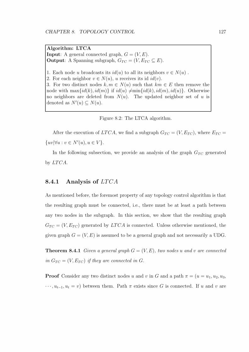
CHAPTER 8. TOPOLOGY CONTROL 127
Algorithm: LTCAInput: A general connected graph, G = (V, E).Output: A Spanning subgraph, GTC = (V, ETC ⊆ E).
1. Each node u broadcasts its id(u) to all its neighbors v ∈ N(u) .2. For each neighbor v ∈ N(u), u receives its id id(v).3. For two distinct nodes k, m ∈ N(u) such that km ∈ E then remove thenode with maxid(k), id(m) if id(u) 6=minid(k), id(m), id(u). Otherwiseno neighbors are deleted from N(u). The updated neighbor set of u isdenoted as N ′(u) ⊆ N(u).
Figure 8.2: The LTCA algorithm.
After the execution of LTCA, we find a subgraph GTC = (V, ETC), where ETC =
uv|∀u : v ∈ N ′(u), u ∈ V .
In the following subsection, we provide an analysis of the graph GTC generated
by LTCA.
8.4.1 Analysis of LTCA
As mentioned before, the foremost property of any topology control algorithm is that
the resulting graph must be connected, i.e., there must be at least a path between
any two nodes in the subgraph. In this section, we show that the resulting graph
GTC = (V, ETC) generated by LTCA is connected. Unless otherwise mentioned, the
given graph G = (V, E) is assumed to be a general graph and not necessarily a UDG.
Theorem 8.4.1 Given a general graph G = (V, E), two nodes u and v are connected
in GTC = (V, ETC) if they are connected in G.
Proof Consider any two distinct nodes u and v in G and a path π = (u = u1, u2, u3,
· · · , ut−1, ut = v) between them. Path π exists since G is connected. If u and v are

CHAPTER 8. TOPOLOGY CONTROL 128
also connected by a path in GTC then we are done. Suppose they are not connected in
GTC . Then we have two connected components G′TC and G′′
TC in GTC . Now π = (u =
u1, u2, u3, · · · , ut−1, ut = v) is divided into two subpaths π′ = (u = u1, u2, u3, · · · , us)
in G′TC and π′′ = (us+1, us+2, · · · , ut = v) in G′′
TC , where us is the last node in π′ in
component G′TC and us+1 is the first node in π′′ in component G′′
TC (see Figure 8.3).
We analyze the following two cases.
u=u1
u2
us+1
us
v=ut
ut−1
G′TC G′′
TC
Figure 8.3: Proving that the subgraph obtained by LTCA is connected.
Case 1: N(us)∩N(us+1) = φ in G. That is, there is no common node between the
neighbors of nodes us and us+1. So, us and us+1 form a clique of size two. Without
loss of generality, assume id(us) > id(us+1). Node us will discard us+1 in GTC if
and only if there is some node k ∈ N(us)∩N(us+1) such that id(us+1) > id(k) (then
us, us+1 and k form a clique of at least three). This is a contradiction since we assume
k does not exist. Therefore, the edge usus+1 is retained in GTC which makes GTC
connected.
Case 2: N(us) ∩ N(us+1) 6= φ in G. That is, there exists at least some node k
such that us, us+1, and k belong to a clique of size at least three. Consider such a
clique C of size p (us, us+1, and k belong to C). In C, we can have at most p − 2

CHAPTER 8. TOPOLOGY CONTROL 129
cliques of three nodes, where us and us+1 are fixed.
According to the algorithm, there are two ways us and us+1 cannot be neighbors
to each other in GTC , namely id(us) 6= minid(m) : m ∈ C \ us or id(us+1) 6=
minid(m) : m ∈ C \ us+1. This is because if either us or us+1 has the smallest
id in one of the p − 2 cliques then the adjacent edges to the smallest id node are not
removed. Thus, if us or us+1 has the minimum id in one of the p − 2 cliques then we
are done.
Suppose none of them has the minimum id. Then it is easy to see that we could
reach us+1 from us via the minimum id node in C. This contradicts the fact that
G′TC and G′′
TC are not connected. Therefore, either π′ and π′′ are connected by edge
usus+1 or there exists a node m ∈ N(us)∩N(us+1) (where id(m) < id(us) and id(m) <
id(us+1)) such that u and v are connected via path π′∪usum∪umus+1∩π′′. Hence,
all pairs of nodes are connected in GTC .
In the following, we prove that the edges in GTC are symmetric, that is, if node
u includes v as its neighbor in GTC , then v includes u ∈ N ′(v). Having the subgraph
symmetric is an important characteristic, because asymmetric communication graphs
are generally hard to realize in practical situations as investigated in [63].
Theorem 8.4.2 Given a general graph G = (V, E) (with uv ∈ E), node u includes
v in N ′(u) if and only if v includes u in N ′(v) in GTC .
Proof We analyze two cases.
Case 1: N(u)∩N(v) = φ. Then according to the last step of LTCA, both u and
v includes the other in their respective updated neighbor list. Therefore, if u includes
v in N ′(u) then so does v.

CHAPTER 8. TOPOLOGY CONTROL 130
Case 2: N(u) ∩ N(v) 6= φ. Consider a common neighbor w ∈ N(u) ∩ N(v).
Assume u includes v in N ′(u). We now show that v also keeps u in N ′(v). Since
v ∈ N ′(u), we have either id(v) < id(w) and id(u) 6=minid(w), id(v), id(u) or
id(u) =minid(w), id(v), id(u) (the relation of ids between v and w does not matter).
For the former situation, if id(v) =minid(w), id(v), id(u) then u is retained in N ′(v)
(step (iii) of the algorithm) and for the latter situation v includes u and discards w
since id(w) > id(u).
To prove the other direction, i.e., v’s inclusion of u in N ′(v) implies v ∈ N ′(u),
simply exchange the role of u and v in the previous paragraph and the proof fol-
lows.
Now we focus on the planar property of GTC since achieving planarity in the
resulting subgraph is one of the expected features in topology control algorithms. The
algorithm does not guarantee that GTC be always planar. However, it can remove a
substantial number of intersecting edges. In the following lemma, we show that all
the intersecting edges of a clique C (|C| > 3) in G can be removed in GTC . This may
greatly reduce the number of intersections in GTC .
Lemma 8.4.3 Let C (|C| > 3) be a clique in G. All the intersections between edges
wx and yz, where w, x, y, z ∈ C can be removed in GTC .
Proof Without loss of generality, let u be the smallest id node in C. According to
LTCA (step (iii)), for any two nodes w, x ∈ C, w and x both will discard x and w from
their respective updated neighbor lists N ′(w) and N ′(x) (since id(w), id(x) > id(u)).
As a result, the edge wx is eliminated from GTC . As all edges wx ∈ E (where w, x ∈ C
and u 6= w, x) are removed, there exist only edges uv, v ∈ C \ u. Therefore, all the
intersections between edges wx and yz, where w, x, y, z ∈ C are removed in GTC .

CHAPTER 8. TOPOLOGY CONTROL 131
However, some edge cd ∈ E, where c ∈ C \ u and d ∈ V \ C can intersect
some edge ab, where a, b ∈ C. Elimination of such intersections is not possible
(with only connectivity information and no geographic location information) without
disconnecting the graph. Situations like the ones shown in Figure 8.4, where the
graphs 8.4(b) and 8.4(c) are indistinguishable from each other (labels indicate the
corresponding ids of the nodes) and hence intersections cannot be removed with only
connectivity information. However, as illustrated in Figure 8.4(a) (right) we can
obtain a planar subgraph from the clique shown of Figure 8.4(a)(left) assuming u has
the lowest id in the clique.
3(b) (c)
2
01
0 3
2 1(a)
z
vx
u
vx
zu
w w
Figure 8.4: Situations like the ones shown in (b) and (c) are indistinguishable fromeach other and hence intersections cannot be removed with only connectivity informa-tion: labels indicate the corresponding ids of the nodes. As illustrated in (a) (right),we can obtain a planar subgraph from a clique (left), assuming u has the lowest id inthe clique.
Theorem 8.4.4 Given a geometric graph G = (V, E), any cycle in the subgraph
GTC = (V, ETC) generated by LTCA has length at least 4.

CHAPTER 8. TOPOLOGY CONTROL 132
Proof The proof can be derived from Lemma 8.4.3.
8.5 Analysis for random graphs
In this section, we study and provide experimental results regarding the sparseness
and spanner properties of the topology GTC . For simulations, we assume that the
underlying graph is a UDG in which the spanner and sparseness properties of GTC
are analyzed. For this purpose, we generate UDGs by placing nodes uniformly and
randomly on a given fixed square and demonstrate the spanner property of GTC for
these graphs. For the sparseness property of GTC , we show that the average degree
of the nodes of this graph is low for each randomly generated UDG, although the
maximum degree of GTC is not bounded. This low degree indicates that GTC is
sparse in the average-case. In Figure 8.5, we show the UDG, the Gabriel graph (GG)
and GTC of 600 nodes placed randomly and uniformly, where the minimum distance
between any two nodes is at least 0.4 unit.
To evaluate the different properties of GTC , we compare it with the GG. Recall
that an edge uv between two nodes u and v in the GG exists if the circle with uv as
the diameter does not contain any other nodes inside it. We choose the GG since it
is one of the most prominent topology control structures which is connected, planar,
energy-spanner and can be locally computed. Hence this is a good candidate for
comparison, specially with respect to the energy-spanner property. Although the GG
is not a spanner in the Euclidean metric (the cost of an edge uv is the Euclidean
distance |uv|), it is an optimal energy-spanner when the metric is an energy metric
(the cost of an edge uv is some power of distance |uv|α, where α is in between 2 and
6).
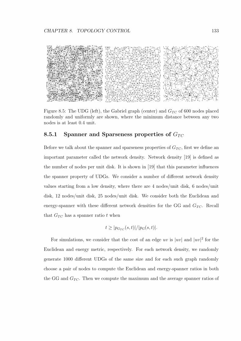
CHAPTER 8. TOPOLOGY CONTROL 133
Figure 8.5: The UDG (left), the Gabriel graph (center) and GTC of 600 nodes placedrandomly and uniformly are shown, where the minimum distance between any twonodes is at least 0.4 unit.
8.5.1 Spanner and Sparseness properties of GTC
Before we talk about the spanner and sparseness properties of GTC , first we define an
important parameter called the network density. Network density [19] is defined as
the number of nodes per unit disk. It is shown in [19] that this parameter influences
the spanner property of UDGs. We consider a number of different network density
values starting from a low density, where there are 4 nodes/unit disk, 6 nodes/unit
disk, 12 nodes/unit disk, 25 nodes/unit disk. We consider both the Euclidean and
energy-spanner with these different network densities for the GG and GTC . Recall
that GTC has a spanner ratio t when
t ≥ |pGTC(s, t)|/|pG(s, t)|.
For simulations, we consider that the cost of an edge uv is |uv| and |uv|2 for the
Euclidean and energy metric, respectively. For each network density, we randomly
generate 1000 different UDGs of the same size and for each such graph randomly
choose a pair of nodes to compute the Euclidean and energy-spanner ratios in both
the GG and GTC . Then we compute the maximum and the average spanner ratios of

CHAPTER 8. TOPOLOGY CONTROL 134
all the 1000 graphs for each network density. Figure 8.6(left) depicts the results of the
spanner ratios of the GG and GTC with respect to the Euclidean metric. The solid
and the dashed lines represent the spanner ratios of the GG and GTC , respectively.
Mean values are plotted in black and max values in gray. It can be seen from the figure
that the GG has a mean spanner ratio which is slightly above 1.1 and the maximum
value is around 1.35. In the same Euclidean metric, GTC has a steady mean around
1.2. However, the maximum is less stable than that of the GG but remains below 7.
We observe that the lower the network density the better the spanner ratio in GTC .
The energy-spanner ratio is shown in Figure 8.6 (right), where the solid and dashed
lines denote the energy-spanner ratios for GG and GTC , respectively. Since the GG
contains an energy-minimal path between any pair of nodes its energy-spanner ratio
is exactly one (mean and max values are the same). GTC has a maximum energy-
spanner ratio as high as 13, but it maintains an average energy-spanner ratio below 1.5
in all considered network densities. In total we ran our simulations on 1000 randomly
generated graphs with different density values that produced the above performance.
We also perform simulations to study the average-case behavior of node degree in
both the GG and GTC . Figure 8.7 shows that the GTC has a better average degree
than that of the GG. For each of the random graphs with a different number of nodes,
the average degree of the GG is always high (at least 3.5), whereas the average degree
of GTC is always below 3.4. Although they are not stable, the gap between them is
significant.
As spanner ratios play an important role in topology control, we wish to see
how our algorithm performs in terms of spanner ratios. Although we plot mean
and max spanner ratios in the energy and Euclidean metrics, they do not reveal the

CHAPTER 8. TOPOLOGY CONTROL 135
5 10 15 20 25
1
2
3
4
5
6
Number of nodes/unit disk
Spa
nner
rat
ios
5 10 15 20 250
2
4
6
8
10
12
Number of nodes/unit disk
Spa
nner
rat
io
Figure 8.6: Spanner ratios of the GG and GTC w.r.t the Euclidean metric (left). Thesolid (resp. the dashed) line represents the spanner ratio of GG (resp. GTC). Meanvalues are plotted in black and max values in gray. Spanner ratios of the GG and GTC
w.r.t the energy metric is shown (right). The solid (resp. the dashed) line representsthe energy-spanner ratio of the GG (resp. GTC). Mean values are plotted in blackand max values in gray. Since the GG contains an energy-minimal path between anypair of nodes its energy-spanner ratio is one (solid line). So its max and mean valuescoincide.
actual performance of the algorithm. In Figure 8.8, we show standard deviations of
the spanner ratios in both metrics. As the network density increases, the standard
deviations of spanner-ratios for both metrics increase significantly. This is because in
dense graphs, generated by high network densities, the algorithm can remove ‘good’
edges which are on the optimal path between two nodes s and v in G. Removing such
edges in GTC can result in paths with cost |pGTC(s, t)| which can be arbitrarily worse
than |pG(s, t)|. Since each node has only minimal information about its neighbors
(only neighbors’ ids) and no knowledge about the distance of their neighbors, it is
not hard to come up with an instance that makes the algorithm perform poorly.

CHAPTER 8. TOPOLOGY CONTROL 136
100 200 300 400 500 600 700 800 900
2.6
2.8
3
3.2
3.4
3.6
3.8
4
4.2
4.4
Number of nodes
Ave
rage
Deg
ree
Figure 8.7: Average degree of the GG and GTC in random graphs of different sizes.The dashed and the solid lines denote the sparseness of the GG and GTC respectively.As can be seen from the figure, the average degree of GTC is always smaller than thatof the GG in all the instances of different sizes of graphs.
8.6 Conclusion
In this chapter, we presented a simple algorithm LTCA for topology control in wire-
less sensor networks which has certain useful properties. This one-hop local algorithm
is very simple, requires only the ids of the neighbors and assumes no geometric in-
formation at all. Each node communicates with its neighbors only twice for sending
and receiving ids and the algorithm terminates after two rounds. Unlike most other
techniques, LTCA does not assume the graph to be a unit disk graph. In fact it works
for all connected graphs since it does not use any geometric information. One funda-
mental property is that it always produces a connected spanning subgraph from the
underlying graph. This property is robust because many existing well-known topol-
ogy control protocols (such as the Gabriel graph, the Relative neighborhood graph,

CHAPTER 8. TOPOLOGY CONTROL 137
0 5 10 15 20 250
1
2
3
4
5
6
Number of Nodes/Disk
Sta
ndar
d D
evia
tion
Euclidean metric
Energy metric
Figure 8.8: Showing standard deviations of spanner ratios of the algorithm for theEuclidean and energy metrics.
the XTC-algorithm) fail to produce a connected subgraph if the exact location infor-
mation of the nodes is not known or there are errors in the estimation of distances
between nodes.
In practical situations, providing precise location information may be expensive
and even challenging and a slight error in the geographic location of nodes results in a
disconnected subgraph. We show that the subgraph generated by LTCA is symmetric
and has few intersections. We provide extensive simulation results for the sparseness
and spanner property in random network graphs. Comparing with the well-known
topology, the Gabriel graph, it is shown that we can obtain good results in terms of
sparseness and spanner ratios in average graphs.

Chapter 9
Conclusion and Future Works
In this thesis, we investigated six different problems in the areas of broadcasting,
routing, data collection, target monitoring, and topology control in WSNs. We pro-
posed a number of novel techniques to address these problems and obtained some
interesting theoretical results which were verified by extensive simulations. However,
the research has also generated a number of interesting open problems which I would
like to study in depth in my postdoctoral research.
In general, researchers need to model a WSN and make some basic assumptions
in order for their algorithms or techniques to work. Often the assumptions made by
most algorithms seem to be unrealistic when applied in real-world situations. For
example, many ‘good’ algorithms assume that sensors know their correct geometric
coordinates when deployed in an extended area, a WSN can be perfectly modelled as
a UDG, etc. In the future, we must start by challenging such ‘strong’ assumptions
and plan to re-investigate some of the ‘well-known’ problems in order to come up
with good solutions. Specifically, we plan to find a technique that does not make
such assumptions, to the problem of generating Connected Dominating Sets (CDSs)
138

CHAPTER 9. CONCLUSION AND FUTURE WORKS 139
which are widely used for routing in WSNs. Finding such a realistic solution would
be a significant contribution to research in WSNs since this can be guaranteed to
function in practical situations.
Once this is possible, we would focus on the quality of the solution, that is, the
size of a CDS. As previously mentioned, the size of a CDS should be as ‘small’ as
possible since smaller-sized CDSs greatly reduce the number of retransmissions and
collisions of messages in the network, which eventually helps increase the lifetime of
sensors. As the problem of obtaining small-sized CDSs is challenging, we will appeal
to advanced combinatorial techniques such as to bound the size of a CDS within a
small constant of the optimum solution.
In this thesis, we introduced a technique to generate a number of CDSs instead
of just one and show that this is a very promising way to reduce the sensors’ energy
consumption to a great extent. In future research, we would be interested in analyzing
this problem in depth to obtain some results about the size of each of the CDSs found
by the algorithm. We believe that bounding the size of each generated CDS could
be possible by carefully utilizing the unique structural properties of UDGs and using
some fundamental graph theoretic results. Furthermore, we hope to conduct large
scale simulations to experimentally evaluate our algorithm.
Another interesting problem called the Domatic Partition problem, which asks
for finding the maximum number of disjoint dominating sets (DDSs) in UDGs, has a
direct connection in increasing the lifetime of a WSN. Although the problem has been
studied in [69, 62], no bound was given on the maximum number of DDSs and hence
it still remains as an open problem. However, we present extensive simulation results
towards solving this problem and based on the convincing simulations together with a

CHAPTER 9. CONCLUSION AND FUTURE WORKS 140
unique property of a UDG namely, a node in a UDG can have at most five independent
nodes in its neighborhood), we conjecture that this problem can be solved within a
constant factor of the optimum.
To this end, we plan to tackle the problem using computational geometric and
graph theoretic techniques such as convex hulls, maximum independent sets. We also
plan to pursue a distributed solution to this problem since distributed techniques are
preferred in WSNs due to their scalability, low overhead and effectiveness.
In a nutshell, we are interested to actively continue our research in the design and
analysis of distributed and local algorithms to the various problems in WSNs. The
main objectives are to explore scalable solutions for practical large sensor networks
that explicitly deal with enhancing the lieftime and other energy issues of the network
and analyze their performance both theoretically and experimentally. We hope this
research will yield results of interest to both the research community and to industry.

Bibliography
[1] K. Alzoubi, P. Wan, and O. Frieder, Message-optimal connected-dominating-set
construction for routing in mobile ad hoc networks, In Proc MobiHoc, 2002.
[2] K. Alzoubi, P Wan, and O. Frieder, New distributed algorithm for connected
dominating set in wireless ad hoc networks, In Proc. IEEE HICSS35, 2002.
[3] K. Alzoubi, P. Wan, O. Frieder, Distributed heuristics for connected dominating
set in sireless ad hoc networks, IEEE ComSoc/KICS Journal on Communica-
tion Networks, 4(1), pp. 22-29, 2002.
[4] S. Basagni, Distributed clustering for ad hoc networks, In Proc. ISPAN, 1999.
[5] J. Blum, M. Ding, A. Thaeler, and X. Cheng, Connected dominating sets in
sensor networks and MANETS, In Handbook of Combinatorial Optimization,
pp. 329-369, 2004.
[6] M. Burkhart, P. Rickenbach, R. Wattenhofer, and A. Zollinger, Does topology
control reduce interference, In Proc. Mobihoc, 2004.
[7] G. Calines and R. Ellis, Monitoring schedules for randomly deployed sensor
networks, In Proc. Dial-POMC, 2008.
141

BIBLIOGRAPHY 142
[8] M. Cardei and D. Du, Improving wireless sensor network lifetime through power
aware organization, ACM Wireless Networks, 11(3), pp. 333-340, 2005.
[9] M. Cardei, M. Thai, Y. Li, and W. Wu, Energy-efficient target coverage in
wireless sensor networks, In Proc. INFOCOM, 2005.
[10] M. Cardei and J. Wu, Energy-Efficient coverage problems in wireless ad hoc
sensor networks, Computer Communications Journal (Elsevier), 29(4), pp. 413-
420, 2006.
[11] J. Carle and D. Simplot-Ryl, Energy-efficient area monitoring by sensor net-
works, IEEE Computer 37(2), pp. 40-46, 2004.
[12] B. Carp, Geographic Routing for sensor networks, Ph.D thesis, Harvard Uni-
versity, 2000.
[13] D. Chen, X. Mao, X. Fei, K. Xing, F. Liu, and M. Song, A convex-Hull based
algorithm to connect the maximal independent set in unit disk graphs, Wireless
Algorithms, Systems, and Applications, pp. 363-370, October, 2006.
[14] X. Cheng, M. Ding, D. Du, and X. Jia, On the construction of connected domi-
nating set in wireless networks, Wireless Communications and Mobile Comput-
ing, vol. 6, pp. 183-190, 2006.
[15] X. Cheng, X. Huang, D. Li, and D. Du, Polynomial-time approximation scheme
for minimum connected dominating set in ad hoc wireless networks, Networks,
42(4), pp. 202-208, 2003.
[16] B. Clark, C. Colborn, and D. Johnson, Unit Disk Graphs, Discrete Mathematics,
vol. 86, pp. 165-177, March 1990.

BIBLIOGRAPHY 143
[17] T. Cormen, C. Leiserson, R. Rivest, and C. Stein, Introduction to algorithms,
2nd Edition, MIT Press, 2001.
[18] B. Das and V. Bharghavan, Routing in ad-hoc networks using minimum con-
nected dominating sets, In Proc. ICC (1), pp. 376-380, 1997.
[19] O. Dousse, P. Thiran, and M. Hasler, Connectivity in ad-hoc and hybrid net-
works, In Proc. INFOCOM, 2002.
[20] U. Feige, A threshold of ln n for approximating set cover, Journal of the ACM,
45(4), pp. 634-652, 1998.
[21] U. Feige, M. Halldorsson, G. Kortsarz, and A. Srinivasan, Approximating the
domatic number, SIAM Journal of Computing, 32(1), pp. 172-195, 2003.
[22] S. Fujita, On the performance of greedy algorithms for finding maximum r-
configurations, In Proc. WAAC, 1999.
[23] S. Funke, A. Kesselman, U. Meyer, and M. Segal, A simple improved distributed
algorithm for minimum connected dominating set in unit disk graphs, ACM
Transactions on Sensor Networks, 2(3), pp. 444-453, 2006.
[24] A. Gallais and J. Carle, An adaptive localized algorithm for multiple sensor
area coverage, Ad Hoc and Sensor Wireless Networks Journal, 3(4), pp. 271-
288, 2007.
[25] A. Gallais, J. Carle, D. Simplot-Ryl, I. Stojmenovic, Localized sensor area
coverage with low communication overhead, In Proc. PerCom, 2006.

BIBLIOGRAPHY 144
[26] M. Garey and D. Johnson, Computers and intractability, a guide to the theory
of NP-completeness, W. H. Freeman and Company, 1979.
[27] S. Ghiasi, A. Srivastava, X. Yang, and M. Sarrafzadeh, Optimal energy aware
clustering in sensor networks, Journal of Sensors, 2(7), pp. 258-269, 2002.
[28] S. Guha and S. Khuller, Approximation algorithms for connected dominating
sets, Algorithmica, pp. 374-387,1998.
[29] C. Gui, P. Mohapatra, Power conservation and quality of surveillance in target
tracking sensor networks, In Proc. MobiCom, 2004.
[30] R. Gupta, J. Walrand, and O. Goldschmidt, Maximal cliques in unit disk
graphs: Polynomial Approximation, In Proc. INOC, 2005.
[31] W. Heinzelman, A. Chandrakasan, and H. Balakrishnan, Energy-efficient com-
munication protocol for wireless microsensor networks, In Proc. HICSS, 2000.
[32] L. Hu, Topology control for multihop packet radio networks, IEEE Transaction
on Communication, 41(10), October, 1993.
[33] K. Islam and S. Akl, Localized topology control algorithm with no geometric
information for ad hoc sensor networks, In Proc. SENSORCOMM, 2008.
[34] K. Islam and S. Akl, A distributed constant factor self-protection algorithm for
wireless sensor networks, In Proc. LOCALGOS in conjunction with DCOSS,
2009.
[35] K. Islam and S. Akl, A localized algorithm for target monitoring in wireless
sensor networks, In Proc. ADHOC NOW, 2009.

BIBLIOGRAPHY 145
[36] K. Islam and S. Akl, Target monitoring in wireless sensor networks: A local-
ized approach, to appear International Journal of Ad Hoc and Sensor Wireless
Networks, 2009.
[37] K. Islam, S. Akl, and H. Meijer, A Simple distributed algorithm for computing
small connected dominating sets in wireless sensor networks, In Proc. ICPADS,
2008.
[38] K. Islam, S. Akl, and H. Meijer, Maximizing the lifetime of a sensor network
through domatic partition, In Proc. LCN, 2009.
[39] K. Islam, S. Akl, and H. Meijer, Distributed generation of a family of connected
dominating sets in wireless sensor networks, In Proc. DCOSS, 2009.
[40] L. Jia, R. Rajaraman, and C. Scheidler, On local algorithms for topology control
and routing in ad hoc networks, In Proc. SPAA, 2003.
[41] R. Karp, Reducibility among combinatorial problems, In Proc. of a symposium
on the complexity of computer computations, 1972.
[42] F. Kuhn, T. Moscibroda and R. Wattenhofer, What cannot be computed locally,
In Proc. Mobicom, 2004.
[43] S. Kumar, T. Lai, A. Arora, Barrier coverage with wireless sensors, In Proc.
Mobicom, 2004.
[44] X. Li, Approximate MST for UDG locally, In Proc. COCOON, 2003.
[45] X. Li, G. Calinescu, and P. Wan, Distributed construction of planar spanner
and routing for ad hoc wireless networks, In Proc. INFOCOM, 2002.

BIBLIOGRAPHY 146
[46] L. Li, H. Halpern, V. Bahl, Y. Wang, and R. Wattenhofer, Analysis of a cone-
Based distributed topology control algorithms for wireless multihop networks,
In proc. PODC, 2001.
[47] X. Li, P. Wan, and O. Frieder, Coverage problems in wireless ad-hoc sensor
networks, IEEE Transactions for Computers, 52(6), pp. 753- 763, 2005.
[48] X. Li, P. Wan, Y. Yang, and O. Frieder, Sparse power efficient topology for
wireless networks, In Proc. ICCC, 2001.
[49] X. Li, Y. Yang, and W. Song, Applications of k-local MST for topology control
and braodcasting in wireless ad hoc networks, In Proc. TPDS, 2004.
[50] X. Li, Y. Yang, P. Wan, and O. Frieder, Localized low weight graph and its
applications in wireless ad hoc networks, In Proc. INFOCOM, 2004.
[51] Y. Li, S. Zhu, M. Thai and D. Du, Localized construction of connected domi-
nating set in wireless networks, In Proc. TAWN, 2004.
[52] K. Lillis and S. Pemmaraju, Topology control with limited geometric informa-
tion, In Proc. OPODIS, 2005.
[53] R. Lin and M. Gerla, Adaptive clustering for mobile wireless networks, In IEEE
Journal on Selected Areas in Communications, 15, pp. 1265-1265, 1997.
[54] N. Linial, Locality in distributed graph algorithms, SIAM Journal of Comput-
ing, 21, pp. 193-201, 1992.
[55] M. Luby, A simple parallel algorithm for the maximal independent set problem,
SIAM Journal on Computing, 15, pp. 1036-1053, 1986.
BIBLIOGRAPHY 147
[56] M. Marathe, H. Breu, H. Hunt, S. Ravi, and D. Rosenkrantz, Simple heuristics
for unit disk graphs, Networks, 25, pp. 59-68, 1995.
[57] T. Moscibroda, Locality, Scheduling, and Selfishness: Algorithmic Foundations
of Highly Decentralized Networks, PhD Thesis, ETH Zurich, Diss. ETH, No.
16740, July 2006.
[58] T. Moscibroda and R Wattenhofer, Maximizing the lifetime of dominating sets,
In Proc. WMASN, 2005.
[59] M. Naor and L. Stockmeyer, What can be computed locally?, SIAM Jounal of
Computing, 24, pp. 1259-1277, 1995.
[60] K. Pahlavan and A. Levesque, Wireless information networks, John Wiley and
Sons, 1995.
[61] D. Peleg, Distributed Computing: A Locality-Sensitive Approach, SIAM,
Philadelphia, PA, 2000.
[62] S. Pemmaraju and I. Pirwani, Energy conservation in wireless sensor networks
via domatic partitions, In Proc. MobiHoc, 2006.
[63] R. Prakash, Undirectional links prove costly in wireless ad-hoc networks, In
Proc. DIAL-M, 1999.
[64] R. Ramanathan and R. Rosales-Hain, Topology control of multihop wireless
networks using transmit power adjustment, In Proc. INFOCOM, 2000.
[65] V. Rodoplu and T. Meng, Minimum energy mobile wireless networks, IEEE
Journal on Selected Areas in Communication, 17(8),1999.

BIBLIOGRAPHY 148
[66] J. Schneider, and R. Wattenhofer, A Log-Star Distributed Maximal Indepen-
dent Set Algorithm for Growth-Bounded Graphs, In Proc. PODC, 2008.
[67] D. Simplot-Ryl, I. Stojmenovic, and J. Wu, Energy efficient backbone construc-
tion, broadcasting, and area coverage in sensor networks, Handbook of Sensor
Networks: Algorithms and Architectures Wiley, pp. 343-379, 2005.
[68] R. Sivakumar, P. Sinha, and V. Bharghavan, CEDAR: a core-extraction dis-
tributed ad hoc routing algorithm, IEEE Journal on Selected Areas in Commu-
nications, 17(8), pp. 1454-1465, 1999.
[69] S. Slijepcevic and M. Potkonjak, Power efficient organization of wireless sensor
networks, In Proc. ICC, 2001.
[70] I. Stojmenovic, M. Seddigh, and J. Zunic, Dominating sets and neighbor elimi-
nation based broadcasting algorithms in wireless networks, IEEE Transactions
on Parallel and Distributed Systems, 13(1), January 2002.
[71] D. Tian and N. Georganas, A coverage-preserving node scheduling scheme for
large wireless sensor networks, In Proc. WWSNA, 2002.
[72] P. Wan, K. Alzoubi, and O. Frieder, Distributed construction of connected
dominating set in wireless ad hoc networks, In Proc. INFOCOM, 2002.
[73] Y. Wang, Personal Communication.
[74] A. Wang and A. Chandrakasan, Energy efficient system partitioning for dis-
tributed wireless sensor networks, In Proc. ICASSP, 2001.
BIBLIOGRAPHY 149
[75] Y. Wang and X. Li, Geometric spanners for wireless adhoc networks, In Proc.
ICDCS, 2002.
[76] Y. Wang, and X. Li, Localized Construction of Bounded Degree Planar Spanner,
In Proc. DIALM-POMC, 2003.
[77] Y. Wang, X. Li and Q. Zhang, Efficient self protection algorithms for static
wireless sensor networks, In Proc. Globecom, 2007.
[78] X. Wang, G. Xing, Y. Zhang, C. Lu, R. Pless, and C. Gill, Integrated coverage
and connectivity configuration for energy conservation in sensor networks, In
Proc. CENSS, 2003.
[79] D. Wang, Q. Zhang and J. Liu, Self-protection for wireless sensor networks, In
Proc. IEEE ICDCS, 2006.
[80] R. Wattenhofer, L. Li, P. Bahl, and Y. Wang, Distributed topology control for
power efficient operation in multihop wireless networks, In Proc. INFOCOM,
2001.
[81] R. Wattenhofer and A. Zollinger, XTC: A practical topology control algorithm
for ad hoc networks, In Proc. WMAN, 2004.
[82] J. Wu, F. Dai, M. Gao, and I. Stojmenovic, On calculating power-aware con-
nected dominating set for efficient routing in ad hoc wireless networks, Journal
of Communications and Networks, 5(20), pp. 169-178, 2002.
[83] , J. Wu, H. Li, On calculating connected dominating sets for efficient routing in
ad hoc wireless networks, In Proc. Discrete Algorithms and Methods for Mobile
Computing, 1999.

BIBLIOGRAPHY 150
[84] Y. Yang, X. Li and O. Frieder, Distributed spanner with bounded degree for
wireless networks, International Journal of Computer Foundations of Computer
Science, 14(2), 2003.

BIBLIOGRAPHY 151
Curriculum Vitae
May 5, 1973 Born in Khulna, Bangladesh
1979-1991 Primary, Secondary and Higher Secondary School in
Khulna, Bangladesh
1992-1996 Studies B.Sc. in Computer Science, Khulna University,
Bangladesh
May 2005 M.Sc. in Computer Science, Queen’s University, Canada
2005-2010 PhD student, research and teaching assistant, Parallel
and Unconventional Group, Prof. Selim G. Akl and
Computational Geometry Group, Prof. Henk Meijer,
Queen’s University
April 2010 PhD, School of Computing, Queen’s University, Canada
Advisors: Prof. Selim G. Akl and Prof. Henk Meijer
Co-examiners: Prof. Prosenjit Bose, Carleton Univer-
sity, Ottawa, Canada
Prof. Ram Murty, Queen’s University, Canada
Prof. Kai Salomaa, Queen’s University, Canada
Prof. David Rappaport, Queen’s University, Canada

BIBLIOGRAPHY 152
Publications
The following lists all publications written during the years of my being PhD stu-
dent at Queen’s University, Canada.
Journal Papers
1. Target Monitoring in Wireless Sensor Networks: A Localized Approach. Kamrul
Islam and Selim G. Akl. To appear in International journal of Ad Hoc and
Sensor Wireless Networks.
2. Planar Tree Transformation: Positive Results and Counterexample. Selim Akl,
Kamrul Islam, and Henk Meijer. Journal of Information Information Processing
Letter (IPL), Elsevier, 2008.
3. Not Being (Super)Thin or Solid is Hard: A Study of Grid Hamiltonicity. E.Arkin,
S.P.Fekete, K.Islam, H.Meijer, J.S.B.Mitchell, Y.Nunez, V. Polishchuk, D.Rappaport,
H.Xiao. To appear in Computational Geometry: Theory and Applications
(CGTA).
4. An Improved Architecture for Cooperative and Comparative Neurons (CCNs) in
Neural Network. Kamrul Islam. To appear in International Journal of Com-
puting. (Special Issue)
5. On Planar Path Transformation. Selim G. Akl, Kamrul Islam, and Henk Meijer.
Journal of Information Processing Letters (IPL), Elsevier, 2007.
BIBLIOGRAPHY 153
Conference Papers
6. Maximizing the Lifetime of a Sensor Network through Domatic Partition. Kam-
rul Islam, Selim G. Akl, and Henk Meijer. Proceedings of the 34th IEEE Con-
ference on Local Computer Networks (LCN), Zurich, Switzerland, 2009.
7. A Localized Algorithm for Target Monitoring in Wireless Sensor Networks.
Kamrul Islam and Selim G. Akl. Proceedings of the 8th International Con-
ference on Ad Hoc Networks and Wireless (ADHOC NOW), Murcia, Spain,
2009.
8. Distributed Generation of a Family of Connected Dominating Sets in Wireless
Sensor Networks. Kamrul Islam, Selim G. Akl, and Henk Meijer. Proceedings of
the Fifth IEEE/ACM Intl. Conf. on Distributed Computing in Sensor Systems
(DCOSS ’09), Marina Del Rey, California, June 2009.
9. A Distributed Constant Factor Self-Protection Algorithm for Wireless Sensor
Networks. Kamrul Islam and Selim G. Akl. 3rd Workshop LOCALGOS, in con-
junction with Proceedings of the Fifth IEEE/ACM Intl. Conf. on Distributed
Computing in Sensor Systems (DCOSS ’09), Marina Del Rey, California, June
2009.
10. A Simple Distributed Algorithm for Computing Small Connected Dominating
Sets in Wireless Sensor Networks. Kamrul Islam, Henk Meijer, and Selim G.
Akl. 14th IEEE Intl. Conf. on Parallel and Distributed Systems (ICPADS’08)
Melbourne, December 8-10, 2008, Australia.
BIBLIOGRAPHY 154
11. A Distributed Algorithm for Computing Voronoi Diagram in the Unit Disk
Graph Model. Yurai Nez Rodrguez, Henry Xiao, Kamrul Islam, and Waleed
Al-Saleh. Proceedings of 20th Canadian Conference on Computational Geom-
etry (CCCG ’08), Montreal, Canada, August 13-15, 2008.
12. Direct Planar Tree Transformation and Counterexample. Selim G. Akl, Kamrul
Islam, and Henk Meijer. Proceedings of 20th Canadian Conference on Compu-
tational Geometry (CCCG ’08), Montreal, Canada, August 13-15, 2008.
13. Localized Topology Control Algorithm with no Geometric Information for Ad
hoc Sensor Networks. Kamrul Islam and Selim G. Akl. Second International
Conference on Sensor Technologies and Applications (SENSORCOMM ’08),
August 25-31, 2008 - Cap Esterel, France.
14. Distributed Construction of Voronoi Diagram in Sensor Networks. Waleed Al-
Saleh, Kamrul Islam, Yurai Nez Rodrguez, and Henry Xiao. ACM Symposium
for Parallel Algorithms and Architecture (SPAA’08) as poster paper, June 14-
16, 2008, Munich, Germany.
15. Hamilton Circuits in Hexagonal Grid Graphs. Kamrul Islam, Henk Meijer,
Yurai Nunez Rodrguez, David Rappaport and Henry Xiao. Proceedings of
19th Canadian Conference of Computational Geometry (CCCG’07), Ottawa,
Ontario, August 20-22, 2007.
16. An Improved Architecture for Cooperative and Comparative Neurons (CCNs) in
Neural Network. Kamrul Islam. International Workshop on Artificial Neural
Networks and Intelligent Information Processing (ANNIIP’07), Angers, France,
May 9-12, 2007. (special journal issue as one of the selected best papers)

BIBLIOGRAPHY 155
17. Planar Tree Transformation through Flips. Kamrul Islam and SM Rafizul
Hoque. Intlernational Conference on Information and Communication Tech-
nology (ICICT’07), Dhaka, March 8-10, 2007.
18. On Planar Path Transformation. Selim G. Akl, Kamrul Islam and Henk Mei-
jer. Proceedings of 18th Canadian Conference of Computational Geometry
(CCCG’06), Kingston, Canada, August 14-16, 2006.